Chaotic lensed billiards
Abstract
Abstract
Lensed billiards are an extension of the notion of billiard dynamical systems obtained by adding a potential function of the form , where is a real-valued constant and is the indicator function of an open subset of the billiard table whose boundaries (of and the table) are piecewise smooth. Trajectories are polygonal lines that undergo either reflection or refraction at the boundary of depending on the angle of incidence. Our main focus is to explore how the dynamical properties of these models depend on the potential parameter using a number of families of examples. In particular, we explore numerically the Lyapunov exponents for these parametric families and highlight the more salient common properties that distinguish them from standard billiard systems. We further justify some of these properties by characterizing lensed billiards in terms of switching dynamics between two open (standard) billiard subsystems and obtaining mean values associated to orbit sojourn in each subsystem.
1 Introduction
Mathematical billiards, particularly in dimension , are dynamical systems of a geometric nature that are relatively easy to define and, at the same time, exhibit a wide range of dynamic properties, making them useful models for more complicated systems. For this reason they have for many decades figured prominently in the development of the modern theory of dynamical systems and ergodic theory. Research on chaotic billiards in dimension , in particular, has by now attained a high degree of technical sophistication. This, in our opinion, justifies an effort to look for generalizations or extensions of the concept of billiard systems that can point to new directions of research without compromising too much on the qualities that make them attractive model systems.
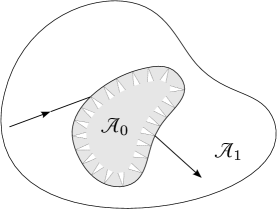
Lensed billiards may be defined as standard billiard systems to which are added piecewise constant mechanical potential functions of the form where is the indicator function of a subset of the billiard domain. We may think of as a scatterer that reflects billiard trajectories that collide with it at sufficiently shallow angles relative to a critical angle to be defined shortly, but allows others to pass through and undergo a refraction, similar to a light ray crossing the interface surface separating two optical media with different refractive indices.
The central new factor to account for is the effect of the potential parameter —the value of the potential function on —on the dynamical behavior of the system. After laying out basic definitions and the most general properties of lensed billiards, the paper focuses on the numerical determination of Lyapunov exponents for a few parametric families of examples, identifies a number of properties that appear to be common for these systems, and proposes a framework of analysis for explaining these common features.
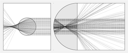
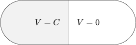
Before embarking on a systematic study, let us get a first impression of what these systems look like. Figure 1 shows two lensed variants of the classical Sinai semi-dispersing and Bunimovich stadium billiards. The shaded regions, let us denote them by , indicate where the potential function is non-zero. In both cases we have set the value of to . The negative potential causes trajectories going into to deflect as if entering an optical medium with higher refractive index. (As a mechanical system, the speed of the point particle naturally increases due to conservation of energy—the opposite of what would happen to a light ray.) Therefore the Sinai scatterer behaves as a focusing lens. The figure on the left shows the typical focusing-defocusing behavior produced by such a lens. On the other hand, trajectories leaving on the Bunimovich-type system on the right-hand side exhibit dispersing behavior after standard focusing inside by the circular part of the boundary. This shows how the choice of values of can alter the standard mechanisms leading to hyperbolicity in billiard systems. If the value of the potential in is positive then these behaviors are reversed. It is easy to verify that if , the system on the left is not ergodic due to trapped trajectories inside the circular lens, and if , the system on the right is not ergodic due to the existence of a positive measure set of initial conditions initiating in the complement of that cannot enter . (We consider initial velocities with sufficient energy to allow the billiard particle to cross the potential barrier, but when the angle of collision with the vertical line of discontinuity of is sufficiently small, the particle is nevertheless forced to reflect.)
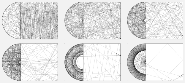
It is important to keep in mind the distinction between the billiard flow and the billiard map dynamics, due to the fact that particle speed is no longer constant. Figure 2 shows the difference in somewhat extreme fashion. As the potential constant on the semi-disc becomes negative with large , the number of steps of the billiard trajectories inside increases, roughly proportionally to (a more precise statement will be given later), suggesting that trajectories of the billiard map become increasingly trapped in that deep potential well. However, the speed of the particle in that region is also proportional to , so the amount of time the billiard flow remains in is expected to remain bounded.
Naturally, the systems we are calling lensed billiards can be viewed as a special case of soft billiards, or more broadly Hamiltonian systems under the influence of a potential, for which there is a rich existing literature that we now discuss. It should be emphasized that the present work takes on related systems from a number of new perspectives. A central focus of soft billiards has been for the case of smooth potentials and for the case of a Sinai billiard table consisting of the torus with circular scatterers. Here, the discontinuous potentials of lensed billiards result in impulse-like forces at discrete times and our examples venture beyond the case of the soft Sinai billiard. There are a number of early examples in the literature whose focus is on characterizing ergodicity under appropriate conditions on a smooth potential in the soft Sinai billiard. In [17], the author shows that for certain bell-shaped potentials under a general smoothness condition ( smoothness at the boundary of the scatterer, among other regularity conditions on the geometry of the table and the total energy of the system), the soft Sinai billiard has the -property and is thus ergodic. Later, in [15], the author shows for a class of smooth Coulombic potentials, again for the Sinai billiard on the torus with disk-shaped scatterers, that the flow of the system can be realized as a complete geodesic flow on a suitably defined compact Riemannian manifold. Under appropriate conditions on the potential, the metric has negative curvature and so the flow is Anosov and hence ergodic. In [11], these results are generalized to a broader class of smooth potentials. Moreover, under certain conditions on the potential, positivity of Lyapunov exponents is shown using Wojtkowski’s method of invariant cone fields. A number of further studies have continued to extend the literature in the case of smooth potentials for the Sinai billiard: exponential decay of correlations and the central limit theorem [2], non-ergodicity and stability of periodic orbits [12, 23], and related questions for tables in higher dimensions [3, 20]. It should be noted that the literature for the case of constant potentials seems to be more limited and confined to the case where the table is the Sinai billiard. In [1] ergodicity is studied numerically and the parameter space, indexed by the scatterer radius and potential magnitude, is delimited into regions of non-ergodicity. Lyapunov exponents [16] and ergodicity [18] have been studied analytically for this example as well. Lensed billiards are also closely related to so-called composite billiards, also known as ray-splitting or branching billiards [4, 14], but are simpler and less of a departure from standard systems.
This paper continues, from a new perspective, the line of investigation of the above mentioned papers. Our work is also motivated by more geometric considerations. The dynamics of geodesic flows on manifolds with discontinuous Riemannian metrics is a potentially interesting topic that, to our knowledge, is still waiting for a detailed study. When the metric tensor is in the conformal class of a smooth metric , that is, for a positive function with discontinuities on smooth hypersurfaces, we have a system very similar to our lensed billiard systems. For more general discontinuous metrics, Snell’s law still holds as shown in [13]. It is hoped that some of the observations about the dynamics of lensed billiards in dimension will serve as a guide into the dynamics of such geodesic flows. (Having this Riemannian setting in mind, some of the details relegated to appendices are given in greater generality than needed for the narrower purposes of the present paper.)
The rest of the paper is organized as follows. Lensed billiard systems are introduced precisely in Section 2. In defining their phase space, a certain care is needed when accounting for refractions. While the systems we study can be considered as a special case of soft billiards with discontinuous potentials, the perspective we take in defining the billiard map has a number of benefits related to the issue of handling refractions and the differential of the billiard map when refractions occur. Just as for ordinary billiard systems, lensed billiards are dynamical systems with singularities. Besides those singularities typically present in ordinary billiards (hitting a corner or grazing trajectories), we should add singular sets caused by the critical angle of incidence, a quantity to be defined formally in Subsection 2.1 that specifies the transition between reflected and refracted trajectories. Subsection 2.1 defines the billiard map of lensed billiards, introduces the notion of the critical angle, and demonstrates the singular sets and phase portraits for a collection of examples to be studied later in the paper. In Subsection 2.2 we make a few observations concerning refractions based on the invariance of the Liouville measure under the lensed billiard map. As a first step in the analysis of lensed billiard dynamics, we describe these systems as a switching process involving two ordinary open billiard systems and obtain mean values for time and number of collisions during sojourns in each subsystem. The idea of switching dynamics and the statistics of sojourn times discussed in Section 2.2 closely links the analysis of lensed billiards with the study of open (standard) billiard systems. (See Figure 8 and the remarks made around it.) In Subsection 2.3 we describe the differential of the lensed billiard map. This is used afterwards to obtain numerically Lyapunov exponents for the examples of parametric families of billiard systems discussed in Section 3, which contains the main results of the paper. The central interest is to explore the Lyapunov exponent’s dependence on the potential parameter . We identify a few properties of lensed billiards that recur in the examples and use the results of Subsection 2.2 to explain some of them.
The authors wish to thank Zhenyi Zhang for pointing out several corrections to an early draft of the paper.
2 Preliminary details and facts
2.1 Definition of lensed billiards
Let be a closed set with piecewise smooth boundary and an open subset of whose boundary is also piecewise smooth. Part of the boundary of may be contained in the boundary of . Let the potential function be for a given constant . The lensed billiard map (and billiard flow) is defined on the phase space of the system, which involves a small modification of the standard billiard phase space definition.
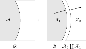
Let and and consider the disjoint union . We fix a value for the total energy (kinetic plus potential). By a regular point in the boundary we mean a point at which the unit vector perpendicular to and pointing towards the interior of at is defined. Note that a piece of boundary common to both and is accounted for twice. These hypersurfaces of discontinuity of the potential function will have a copy as part of the boundary of and another as part of the boundary of . Since these are sets where refracting is possible, we say that they are contained in the refracting boundary. The others that are not duplicated are part of the reflecting boundary.
The phase space of the billiard map is the set of pairs where is a regular point in the boundary of and is a tangent vector at such that and
We define the billiard map
as follows. Suppose . Let If is not a regular boundary point, the billiard map is not defined. If it is regular, let , , be the corresponding point in . Set . We now determine whether the new velocity should be defined by a reflection or a refraction of . We say that the angle between and is critical if the normal component of satisfies
Equivalently, this happens for the angle that satisfies:
| (1) |
Note that a critical angle of incidence is only possible when ; that is, when approaching a region of higher potential from a region with lower potential. The state corresponding to a critical angle of approach is then included in the singular set of the billiard map and the trajectory is terminated. If the velocity vector undergoes a reflection, we set (recall ); if it undergoes a refraction, then , .
In order to define , let be the orthogonal decomposition of at . The tangential component of the new velocity in both cases is
and the normal component is
This rule for obtaining is easily justified, for example, by introducing a smooth potential transition over a narrow tubular neighborhood of the line of discontinuity of width , then taking the limit of the solution to Newton’s equation of motion as approaches . We relegate the details (of a more general fact) to Appendix A.1.
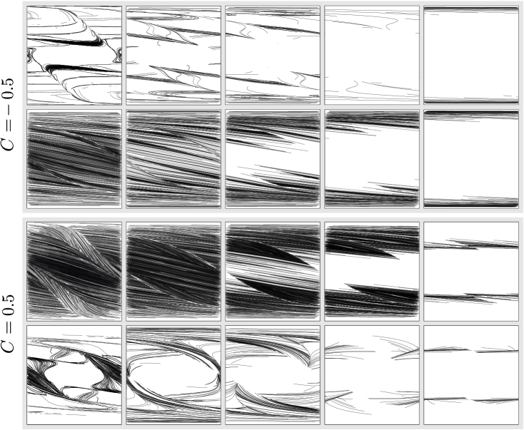
It would be possible, under a convexity assumption, to define the billiard map when the angle of incidence is critical, but we choose to exclude states leading to such angles from the domain of definition of the billiard map. States in whose orbits generated by the map , after a finite number of steps, lead to a critical angle or to a non-regular point of , or to tangential contact, will be called singular. The billiard table in Figure 4 will be used as a multiparameter family of examples at a number of places. For this example, Figure 5 illustrates the points in the singular set associated to critical angles. These are the new critical points not present in standard billiards.

The figure only shows the part of the phase space over the vertical segments on the right end of the rectangular domain. Further details are given in the figure’s caption. Figure 6 shows a few phase portraits of examples taken from the family of Figure 4. The plots only show orbits of the return map to the right vertical side of the rectangular domain.
It will be assumed (as it is often done for standard billiard systems) that the domain of in is an open set of full Lebesgue measure and that is a smooth map there. This will be valid for the examples in this paper.
2.2 Switching dynamics and measure invariance
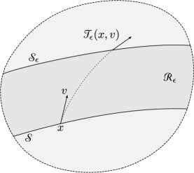
A prominent aspect of the dynamics of lensed billiards is the back-and-forth switching process between two standard billiard systems in and . Segments of trajectories from the moment of arrival in region to the moment of the next switch back into the other region will be called sojourns. The statistics of time and number of collisions during a sojourn plays a role in the analysis of lensed billiards, as will be seen. We give in this section the mean value of these two quantities under the assumption that the two standard billiard subsystems are ergodic.
It is useful throughout to keep in mind the mechanical counterpart of Snell’s law. Recall from the definition of the refraction map given earlier that, upon refraction at a point of discontinuity of the potential, the components of the incident and transmitted velocities tangent to the line of discontinuity are equal. If the trajectory leaves and enters , , and if and are the angles of the velocities and pre- and post-refraction, respectively, relative to the unit normal vector to the line of discontinuity pointing into , then equality of tangential velocity components amounts to It follows that
This is Snell’s law, in which terms of the form assume the role of the refractive index in geometric optics.
A few remarks will be needed concerning invariance of the canonical billiard measure. If is the potential function on and is the billiard phase space, let consist of the points in such that . This is the invariant subset of states with total energy . Denoting by the angle between and , and by the arclength parameter along boundary line segments, the canonical billiard measure, or Liouville measure, is the measure on such that
| (2) |
It is well-known that this measure is preserved by the billiard map. That the lensed billiard map also preserves this measure is briefly justified in Appendix A.2. We refer to the angle distribution in as the cosine law.
We note the following effect of the square root term appearing in Equation (2). The invariant measure on the part of the lensed billiard phase space corresponding to an interface segment between regions with potentials and is proportional to on the side of potential value and on the other side. Thus in the long run, for an ergodic system, the ratio of probabilities of transitions into (from either or ) over transitions into is
Let us illustrate this point using the lensed variant of the Bunimovich stadium shown in Figure 7, which may be expected to be ergodic, although we do not verify it here.
Let us focus on the vertical interface line in the middle of the table. The probability that the particle, upon reaching the vertical line (from the left or from the right), will continue towards the right by either reflection or refraction () over the probability of continuing towards the left () should be (taking mass and energy )
In particular, when is negative and is very large, this probability is close to . This means that once the particle falls into the region of negative potential, most “collisions” with the vertical line correspond to reflections on the left side. The opposite holds when lies between and and close to . As an illustration, the following table gives predicted values and values obtained by numerical simulation for a randomly chosen orbit of steps.
Comparing two boundary segments in a region with same value for the potential, the ratio of the number of crossings of the vertical segment from right to left over the number of collisions with the horizontal segment of the same length in the region where the potential is (chosen equal to in the simulation, for a trajectory of steps), was , to be compared with the exact value .
Another manifestation of measure invariance is recorded in the following proposition. (See Appendix A.2 for further remarks.)
Proposition 1.
Suppose . Let be a regular point and the unit normal vector to at pointing into . Further suppose that the velocity of trajectories incident upon at coming from is distributed according to the cosine law. Then the distribution of post-crossing velocities, conditional on the occurrence of refraction, also satisfies the cosine law.
A standard application of the Ergodic Theorem (see Appendix A.3 for more details) gives the next proposition, for which we use the following notation. Let be either or . Let and be the area and the boundary length of , respectively, and . Denote by the length of , by the length of the boundary of and by the area of . Let be the space of pairs where and is a tangent vector to at pointing into and having norm . Similarly, we denote by the space of pairs where now . At each , let and denote, respectively, the time of first return to and the number of collisions with the boundary of of a billiard trajectory with initial state before returning to . For each , let denote the time duration of free flight from to the point of next collision. This is naturally the length of the free flight divided by the speed . Finally, denoting by and the normalized Liouville measure on and , respectively, we introduce the mean values
Proposition 2.
With the notations just introduced and under the assumption that the standard billiard map in is ergodic, the following relations hold:
-
1.
;
-
2.
;
-
3.
-
4.
Furthermore, if consists of pairs such that and the angle which makes with the normal satisfies then the mean number of returns to before a first return to is .
Let us assume for concreteness that . Transitions from to happen whenever the trajectory reaches the separating hypersurface, at any angle of incidence. On the other hand, transitions from to can only occur when the angle of incidence between the velocity vector and the normal to the separation line (pointing into ) is smaller than the critical angle. Denoting by the angle of incidence, a transition from to happens when . (See Equation (1).) Furthermore, by Snell’s law, the angle that the trajectory makes with the same normal vector as it crosses into satisfies
| (3) |
Corollary 3.
Suppose the value of the potential function in is with and that the standard billiard system in is ergodic for and . Let and denote the mean time and number of collisions of the lensed billiard system during a sojourn in before the next switch to the other region. Then
where and are the area of and the length of the boundary of .
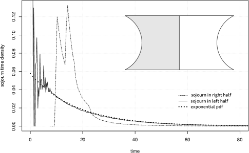
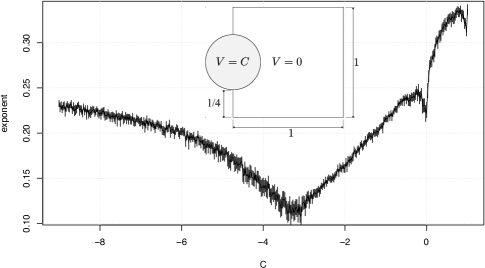
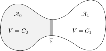
Further information about the probability distribution of sojourn times, beyond simply their mean values, is a focus of future study. For an example of what can be expected, consider Figure 8. It shows the sojourn time distributions for the lensed billiard system whose billiard domain is shown in the figure inset. The left half of the table has potential and the right half has potential , while the total energy of the billiard particle is a small positive value. Thus the particle undergoes many more collisions in a typical sojourn in the left-hand region. In order to cross back into the right-hand region, the billiard trajectory has to pass through a window in phase space defined by the vertical middle line and a small angle interval. It is interesting to note, in particular, the tail behavior for the sojourn time distribution in the left half, which is well approximated by the probability density of an exponential random variable with parameter equal to the reciprocal of the mean sojourn time.
It is likely that methods for the study of open billiards such as in [6] and [19] can be used for a detailed analysis of sojourn time distribution in potential wells. In lensed billiards we are presented with two ordinary billiard systems that are open to each other in the sense that the phase space of each contains a subset, or hole, through which the billiard particle can cross into the other. The size of the hole is smaller for the region with smaller potential. One should expect the successive hitting times, appropriately normalized, into small holes to be approximated by a Poisson process for hyperbolic billiard subsystems.
2.3 Differential of the lensed billiard map
We wish here to obtain the differential of the lensed billiard map to be used in the next section for the evaluation of Lyapunov exponents. For this purpose we introduce coordinates that differ in minor ways from the more commonly employed conventions. The main difference is that, instead of the Jacobi coordinates adapted to wavefronts in a neighborhood of as in the standard reference [8], we use arclength parameter along the boundary curves of and angles that are measured relative to itself. The differential of the billiard map at reflections will differ from the more standard description by the absence of a cosine term at certain places. This small deviation from standard conventions has been made in order to avoid having to elaborate on the behavior of wavefronts at refractions. For standard billiards, time and arclength parameters are everywhere proportional since particle speed is constant, but this is no longer the case across refractions, which introduces a few issues that we choose to avoid.
Recall that the smooth pieces of the boundary of are the pieces of the boundaries of and oriented so that the unit normal vector field points towards the interior of . Let be the unit tangent vector field to the boundary chosen so that is a positive orthogonal basis at each regular boundary point. Let us consider one step of the billiard trajectory from in boundary piece to in boundary piece . The initial velocity is such that (standard dot product) and . This is shown in the diagram of Figure 9 where, on the left, produces a refraction and on the right a reflection.
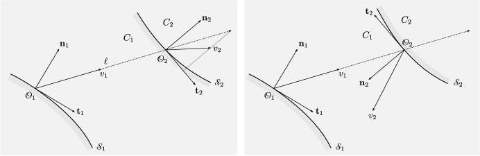
Let denote the rotation matrix in by counterclockwise. This is the generator of plane rotations: the linear map rotates counterclockwise by angle . Thus for a small interval of angles centered at , this defines a neighborhood of velocities centered at . We define coordinates in a neighborhood of and in a neighborhood of so that any in the first neighborhood and in the second satisfy:
| (4) |
We wish to obtain the differential of at :
The following additional notation is needed. Let denote the geodesic curvature of , which is defined by
where indicates standard directional derivative of vector fields along . Let be the Euclidean distance between and , and set , . Further write for the total energy (kinetic plus potential) and , for the values of the potential at the regions indicated in Figure 9.
Theorem 4 (Differential of the lensed billiard map).
With the notations just given, the differential in the coordinate systems is given by
if a reflection occurs at or
if a refraction occurs. In the latter case,
The determinant of is in both cases.
The similarities between the differentials for reflection and refraction become more apparent with the following notation: where we recall that . Then
3 Numerical study of Lyapunov exponents
In this section we wish to explore, mainly numerically, the ways in which the presence of lenses affects the billiard dynamics as measured by the Lyapunov exponents of the billiard flow. Thus we are concerned with the following quantity:
where is the time elapsed up to step .
Due to invariance of the Liouville measure (which is associated to an invariant -form on phase space) we know that, on ergodic components, exponents come in pairs . We refer to the nonnegative value as the Lyapunov exponent of the system. In the numerical experiments shown here, we compute the average of over a large sample of randomly chosen initial conditions. Not all the examples considered are ergodic, so the numerically computed may involve an average over the values on ergodic components. Also note that exponents are obtained numerically using the differential of the billiard map described in Section 2.3.
In all cases, we set the mass parameter and particle total energy . Thus particle speed in regions where the potential is equals and a region on which the potential value is greater than or equal to acts as a standard billiard scatterer; that is, the boundary of becomes part of the reflecting boundary.
We identify a number of common features specific to lensed billiards among the examples considered here. We also provide conceptual explanations for some of these features based on the results of Section 2.2. The present discussion is exploratory in nature and the explanations for the observed features are heuristic and informal, although we expect they will serve as a basis for a more detailed study to be pursued elsewhere.
3.1 A multiparameter billiard case study
Let us consider first the multiparameter family depicted in Figure 4. We wish to use it to illustrate a number of properties that seem to be typical of lensed billiards but distinct in comparison with standard (purely reflecting) billiards.
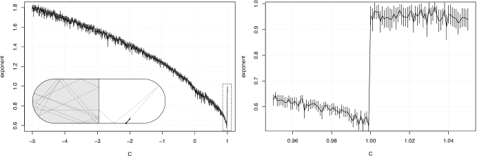
As a first experiment, let us obtain approximate values for the positive Lyapunov exponent as a function of the curvature parameter when , initial speed is , and . Since , this is a standard billiard system on the region where the potential is . This will serve as a basis for comparison when setting .
The results are shown in Figure 10. Negative values of correspond to semidispersing billiards and positive values to focusing billiards. For each of equally spaced values of we compute the mean value for the exponent over a sample of orbits of length with random initial conditions: points are taken from the vertical wall on the right with the uniform distribution and velocities according to the cosine law density. Whiskers represent confidence intervals based only on the sample variation of the simulated data. Other potential sources of errors may not be accounted for in this and similar graphs.
It is worth noting the distinct nature of the graph over the interval . (The dashed vertical line is at .) The upper limit of this interval is the curvature for which the center of the circular arc lies on the vertical right wall. The less well-defined behavior in the range is likely due to breakdown of ergodicity. In fact, for , the billiard is semidispersing, hence ergodic. For , Bunimovich’s condition (see [5]) for ergodicity based on defocusing in nowhere dispersing billiards holds. This observation offers a clue to help identify lensed billiard systems that fail to be ergodic in parametric families, although we do not pursue the determination of ergodicity (or failure of ergodicity) in detail in the present paper except to note it in some obvious cases.
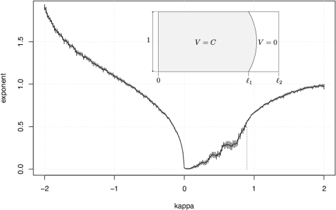
Let us now investigate the effect of setting . Figure 11 refers to the same family as in Figure 4 (or Figure 10) except that the fixed parameters are , , on the left and , , on the right. The potential is the parameter to be varied. Comparison with the previous graph suggests a discontinuity at (which corresponds to a standard reflecting billiard system.) Sample sizes and orbit length for each value of are as in the previous experiment. For and , a fraction of arrivals from the right at the line of potential function discontinuity undergoes dispersing reflections. This and the sharper appearance of the graph in that range may indicate that the system is ergodic and that for it is not.
Referring now to the system associated to the graph on the right of Figure 11, for negative , the billiard particle can become momentarily trapped in the shaded region of Figure 4, where it behaves as in a semidispersing billiard. This suggests that for and this lensed billiard may be ergodic. We see again, by comparison with Figure 10, a discontinuity at . An explanation for the jump discontinuity will be provided shortly.
Another feature that can be noted on both graphs and others shown later is the presence of a local maximum for positive values of less than but close to the point of exponent discontinuity (). We will have more to say about this shortly.
For the exponent grows with . We leave a detailed proof of this and other remarks to a future paper. However, the following elementary observation can be adduced to justify this claim. Let denote the number of collisions with the boundary of the shaded region (Figure 11 on the right) that a trajectory with initial state undergoes during a sojourn in . Let denote the corresponding time of that sojourn. Now consider
As , both and grow to infinity for almost all . It can be expected that the limit on the left will be the exponent for the billiard flow while the limit on the right will be the product of the exponent for the billiard map times the limit of . Under the assumption that the system is indeed ergodic for negative , this quotient converges to which, by Proposition 2, is , where is the perimeter of , is its area, and .
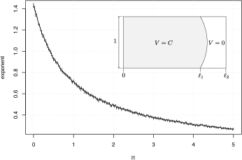
The dependence on the geometric parameter is particularly simple. In Figure 12 we set , , , and let range from to . A fairly regular dependence of the exponent on the varying parameter is now observed. This is easily explained by noting that the number of collisions contributing to the exponent is independent of , while the time spent in the region where () is proportional to .
It was observed in the examples that the exponent has a jump discontinuity, as a function of , at the point of transition from lensed to purely reflecting billiard. Let us, informally, estimate the size of the jump. We only provide here a heuristic argument, based on Proposition 2 and Corollary 3. (See the example of Figure 14 for a bit of numerical evidence.)
Suppose the standard billiard systems in the closures of and are ergodic. Let be the Lyapunov exponent of the lensed billiard flow on for which and . Let denote the positive exponent when . That is, the exponent for the standard billiard flow in , where . Then, as approaches , we expect
to hold, where is the area of . In the example of Figure 14, the two areas are equal, therefore as the limit exponent is expected to be half the value it assumes for . This is very nearly what the numerical example shows. (See the right-hand side of that figure.)
To explain this feature, let us first introduce some notation. Let be the return map to (the intersection of the boundaries of and ) after moving into . Let be the number of returns to before a trajectory that enters finally switches to . Thus corresponds to a sojourn into whereas a sojourn into involves applications of . For each positive integer , let
Let us fix a typical orbit, beginning with a entering :
Note that . Times and number of collisions in each sojourn will be written and for . The total time after sojourns in and sojourns in is
where we have defined
We similarly define for the number of collisions after sojourns in and . Let be a vector defining an infinitesimal variation of the initial condition . We write and, inductively,
Then, omitting reference to to simplify the notation,
Focusing attention first on the first summand on the right side of the above equality, the following is expected to hold: the quantity in parentheses is almost everywhere finite, the quotient converges to an area ratio based on Proposition 2 and Corollary 3 and, due to the same proposition, should go to . The second term contains the quotient which, by Proposition 2 and Corollary 3 should limit to . Finally, the quantity in parentheses should converge to the exponent .
Summarizing common features of lensed billiards Lyapunov exponents observed so far:
-
•
There exists a discontinuity of the Lyapunov exponent as approaches the total energy , that is, at the transition from lensed to standard (purely reflecting) billiard.
-
•
In the examples considered so far, the exponent grows as . Different asymptotic behavior will be noted in the additional examples of Section 3.2.
-
•
For values of less than but close to , the exponent has a local maximum as a function of . This common feature is more subtle and its explanation requires a more detailed analysis. See further remarks in Section 3.3.
3.2 Variations on Bunimovich and Sinai billiards
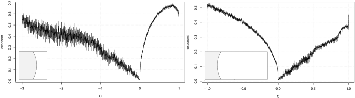
Let us consider here a few more examples from different parametric families in which is the sole parameter, beginning with the variant of the Bunimovich (half-) stadium shown on the left of Figure 13. The positive Lyapunov exponent is given as a function of the potential function parameter . The standard stadium billiard corresponds to .
We notice greater sample variance for . In this range, the billiard system is not ergodic. In fact, when the initial position lies in the unshaded square region where the potential is , and the initial velocity is such that the first collision with the vertical line of potential discontinuity is greater than the critical angle, the trajectory must remain in that region since the normal component of the velocity is not large enough to overcome the potential barrier.
On the right of Figure 13 we have a lensed version of Sinai’s semidispersing billiard in a square with reflecting boundary. (One should compare this graph with that on the left of Figure 11.) For all the lensed Sinai billiard is not ergodic since there is a positive measure of trajectories that are trapped inside the circular lens. The condition for being trapped is that the angle which the initial velocity makes with the inner normal vector to the circle be less than the critical angle.
It will be explained shortly that, in the limit as , the Lyapunov exponent for the system on the right for trajectories started in the region of potential is expected to converge to the exponent of the Sinai billiard, corresponding to . We haven’t determined the asymptotic behavior of the graph on the left for .
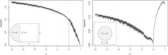
Figure 14 refers to the lensed half-stadium billiard shown in the inset of the graph on the left. It shows a billiard trajectory for strongly negative . A billiard trajectory originating from the right side of the stadium must fall into the shaded region at the moment of first arrival at the separating vertical line, and the velocity after crossing must be nearly perpendicular to the line. Note the growth of the exponent for negative for large values of . In these experiments the particle was initiated on the right side of the stadium with speed . When it moves to the left side, it acquires a large speed, so the exponential rate of growth of tangent vectors increases accordingly; the exponent should be growing proportionally to as . On the right: zooming in near shows more clearly the discontinuity at . As expected (given that the two sides of the billiard table have equal area), the jump discontinuity amounts to a near doubling of the exponent.
Let us turn now to the family shown in Figure 15. This lensed system may be viewed as an interpolation between a focusing billiard, when , and a semidispersing billiard, when . One observes several regimes of behavior over different ranges of the potential parameter : one regime between and (with a discontinuity at ), one between roughly and , and one for less than approximately . On this last range, the exponent grows very slowly as increases and appears (for very large values of far outside the range of the graph) to stabilize near , which is roughly the value of the exponent for . This apparent coincidence will be explained in Subsection 3.4.
3.3 Local maxima
Let us now return to the presence of local maxima for the Lyapunov exponent as a function of the parameter . This ubiquitous feature is seen especially clearly in the graph on the right-hand side of Figure 13, over the interval , for the Sinai lensed billiard system. The following comments apply to this system. Though short of constituting a proof, they contain key ingredients needed for a detailed analysis under more general conditions. We leave this analysis to a future study.
When , the circular lens has no effect on the motion of the billiard particle and the Lyapunov exponent is . It seems clear that, as increases from , exponential separation of trajectories should follow due to both (dispersing) reflections and refractions. What is needed then is an explanation for the observed decrease of the Lyapunov exponent as increases to for small values of .
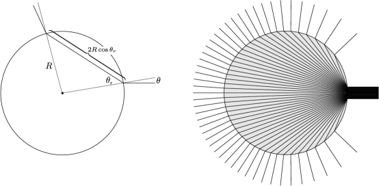
We suppose, for the sake of arriving at a rough estimation, that particle collisions with the lens are statistically independent of each other and the angle of incidence is random and satisfies the (cosine) distribution . An elementary calculation yields probability for a collision to result in refraction, where is the total energy. The expected expansion rate (of separation of nearby trajectories) in the event of a refraction turns out to be proportional to . This is the result of an elementary but long calculation, which we omit. However, this large value, when is close to , is easily understood since the particle will undergo a refraction if the angle of incidence is very small, specifically , but it fans out inside the lens over the full range with the cosine law distribution. (See Proposition 1.) Figure 16, on the right, illustrates the situation.
The contribution of the motion inside the lens to the total time elapsed over a large number of collision events (reflections and refractions) does not depend on . In fact, on one hand, the average time spent inside the lens during one refraction event is easily shown to be . This is obtained by noting that the time the segment of trajectory that enters the lens with angle spends inside is
where is the refracted angle obtained from by Snell’s law (see Figure 16); by Proposition 1 once again, has the cosine distribution. The mean value is then an easy integral calculation. On the other hand, the proportion of refracting collisions is , so the term cancels out, giving the value . Thus refractions contribute over many collisions an expansion rate per collision proportional to
whose logarithm decreases to as approaches from below. To this should be added a term that contains the contribution to the Lyapunov exponent due to reflections, which is obtained by standard geometric calculations. The result is an expansion factor which, for small , has the form
where is a positive quantity that does not depend on , is the mean time of motion outside of the lens between two consecutive returns to the lens, and is the already defined fraction of time of motion inside the lens. Its presence in the denominator explains the previously noted discontinuity of the Lyapunov exponent at . We conclude that, for small values of and under the simplifying independence assumption made above, the Lyapunov exponent is expected to decrease to a limit value as increases towards .
The mechanism suggested here does not account for the second local maximum seen in the example of Figure 15, in the range , close to . A different analysis is needed, which we won’t carry out here.
3.4 Deep potential well limit
The examples of lensed billiards discussed in this paper suggest that exploring the asymptotic properties of the exponent as may be a fruitful direction for further study. One may ask, in particular, whether there are dynamical systems that realize the limit in some sense. The term deep well systems will be used to refer to lensed billiards with strongly negative or to the limit systems when they can be meaningfully specified.
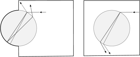
Let us first look at circular lenses as in the examples of Figure 15 and the right of Figure 13. We refer first to the left of Figure 17. As tends to , a trajectory entering the circular potential well is deflected by refraction towards the radial direction and returns, after a very short time interval (since the speed is very high inside the disc), to a point on the circle which is very close to that from which it entered the circle. The angle relative to the normal vector at which the trajectory reaches the right semicircle in the lens boundary after one reflection with the left semicircle is the same as the angle at which the trajectory enters the disc. Therefore the trajectory leaves the disc at the moment of first return to the left semicircle. Furthermore, the velocity with which the trajectory exits the circle is very close to what it would be under specular reflection at that point. Effectively, the system behaves in the limit as that for which . The limit trajectory is shown in the figure as a dashed line. The duration of the sojourn inside the disc (moving along the radial direction) is zero. Thus it makes sense to say that the limit system is the Sinai-type semi-dispersing standard billiard.
The same argument applies to the lensed Sinai billiard on the right of Figure 17. Here, the deep well limit can be described as follows. Let be the billiard map of the Sinai billiard in a square with reflecting sides. Let be the rotation of the plane by , where the origin is placed at the center of the disc. Note that these two maps commute and that is the identity. Then, disregarding the radial segment of trajectory inside the disc (whose duration is ), the limit system is generated by the map .
When the lens region is such that the standard billiard system in it is ergodic, the deep well limit may best be described as a random dynamical system of the following type. We assume for concreteness that the particle mass is and the total energy is . Let be the area of and the length of the intersection of the boundaries of and . Set . Referring to Figure 18, the random system will then be a billiard-like system in that reflects specularly on the part of the boundary not including and, on reaching , trajectories jump to a point and assume velocity such that are random variables distributed according to the Liouville measure: uniform distribution for and the cosine law distribution for . The jump is not instantaneous but happens with a random time delay with mean . If the closed billiard system in is hyperbolic, one may expect this random time to be exponentially distributed. This possible description of a deep well billiard limit is motivated by Corollary 3 and Proposition 1, as well as the example of Figure 8.
Appendix A Appendices
A.1 Motion under discontinuous potential
In order to justify on physical grounds our definition of the lensed billiard map, it will be useful to see how trajectories under discontinuous potentials arise in the limit of a family of smooth potential functions with increasingly sharp transition between two constant values. We do this in the setting of Riemannian manifolds of arbitrary dimension.
The following considerations will be local in nature. Suppose that the potential function , restricted to a neighborhood in the Riemannian manifold with a smooth metric , has only two values, and . The discontinuity of lies on a smooth hypersurface , and is the union of open sets and such that . We make the assumption that . The discussion in this section applies to the opposite inequality with minor modifications. Let be a unit vector field on , perpendicular to , and pointing into . Define for the set
Then is the union of submanifolds consisting of the points in in which and is constant. Note that . The vector field can be extended to all of by setting where and . It is not difficult to show (this is essentially Gauss’s lemma, [7]) that is perpendicular to at any . Clearly since the integral curves of are geodesics. (Here denotes the Levi-Civita connection.)
We define a smooth potential function on as follows. Let be a smooth real-valued increasing function such that
Now set
| (5) |
Let denote the shape operator of the level hypersurfaces . Thus, by definition,
for all . Finally, if , the orthogonal decomposition of into a tangent vector to the hypersurface containing and a perpendicular vector will be written as
Lemma 5.
Newton’s equation in with potential function as defined in Equation (5) decomposes orthogonally as
Proof.
Since , we have
Let denote the orthogonal projection to the tangent space at to the hypersurface containing . Then
Separating the normal and tangential parts we obtain and the desired equations. ∎
Lemma 6.
We make the same assumptions as in Lemma 5, except that now we require to be constant equal to on and constant equal to on . Let the initial velocity of a particle that enters from be and let the velocity upon exit from be for the discontinuous potential function and for the potential . Further assume that the shape operator of the hypersurface is bounded. Then and the return time to the boundary of is .
Proof.
We consider the case . The opposite inequality can be argued similarly. Thus is increasing along the radial direction (parallel to the vector field ) in . Energy conservation implies
for all . We are only concerned with the trajectory from to , when it reaches again the boundary of at a point where . (The case in which the trajectory does not overcome the potential barrier and returns to the boundary of can be dealt with by similar arguments.) Thus we know that
where is an upper bound on the norm of the shape operator. By Lemma 5,
Note that , so Integrating in gives
This quantity is bounded away from for . Explicitly,
in that interval. Then
Setting , we can be certain that the trajectory will reach the boundary of (on the side of ) at in time and that
This shows that
It is now a simple consequence of Lemma 5 that
| (6) |
Therefore as claimed. (More properly, one may write the first equation in Lemma 5 as a system of first order non-linear equations in the components of with respect to an orthonormal parallel frame of vector fields along a trajectory . The approximation given above in (6) is easily shown to hold for these components.) ∎
A.2 Invariant lensed billiard measure
Let us begin by recalling a basic fact about the invariance of the canonical (Liouville) measure under the billiard map. Suppose is a Riemannian manifold of dimension with piecewise smooth boundary and is a potential function which is bounded from above. We assume for the moment that is smooth and let be the billiard map on the phase space . (When is smooth, the set plays no role and and are the same.) We fix a value for the total energy such that is bounded from below by a positive number and let denote the level set of the total energy function for the value . Thus
The canonical billiard measure, or Liouville measure, is the measure on obtained by the restriction to of the volume form derived from the symplectic form on the tangent bundle of . Let us denote this measure by . It is a classical result that this measure is invariant under the billiard map.
More generally, if is a codimension submanifold in the interior of , we can redefine so that it is the map defined over the union of the boundary of and and, upon reaching , the velocity of the billiard flow is not reflected. We have in mind to apply this fact to that are level sets of .
Let (a point in the phase-space of the lensed billiard) be such that is a regular point in a smooth boundary piece of and where is the normal vector field on pointing to the interior of . Thus represents the state of a billiard particle arriving at a point of discontinuity of the potential. We suppose that the normal component of is sufficiently large for the billiard flow trajectory to overcome the potential barrier and cross into . Let be the base-point projection and a neighborhood of such that consists of regular points and velocities leading to refraction.
Our goal is to show that the lensed billiard map preserves the canonical measure . For this it is enough to show that the refraction operation itself preserves the measure. It will be convenient to denote this operation by even though it does not involve the displacement which, together with the reflection or refraction, makes up the billiard map as defined in Section 2.1. Let be the value of the potential function on . As in Appendix A.1, we approximate the potential step by a smooth transition over a narrow band bounded by and . This is indicated in Figure 19. Thus has value on and on , and it is defined by means of a function according to the construction used in Appendix A.1. Let
be the map induced by the Hamiltonian flow. (See Figure 19.) Note that limits to in while in it limits to the subset of the boundary of corresponding to as approaches ; and should be viewed as contained in the boundary of . Thus in the limit we distinguish , contained in the domain of and , contained in the range of . Finally, let denote the canonical measure on . Note that measure invariance under the Hamiltonian flow implies , where is the push-forward operation on measures.
With these notations, proving invariance of the canonical measure under the lensed billiard map reduces to showing the following. For any given continuous real-valued function with compact support in ,
as . On the other hand, the left-most term above converges to
Therefore
This implies invariance of the canonical measure under refraction. We thus arrive at the following.
Theorem 7.
The lensed billiard map preserves the Liouville measure.
The invariant measure can be given the following concrete form. (See [10].) Let denote the Riemannian volume measure on the boundary of and the Riemannian measure on the hemisphere
Then, up to multiplicative constant,
In particular, the distribution of directions has density (relative to the Riemannian volume on the unit hemisphere) given by the cosine of the angle between and .
Proof of Proposition 1.
In this general Riemannian setting, Proposition 1 can be proved as follows. Let be the hemisphere centered at consisting of unit vectors such that , and let be the unit disc in the tangent space . Let be an orthonormal basis of and let denote coordinates of points in relative to this basis. If we parametrize using these coordinates, the volume element on the hemisphere satisfies where is the angle between and . In other words, the cosine law corresponds to uniform distribution in . The set of trajectory segments arriving at from whose velocities undergo refraction are those for which . Under the given parametrization of by , this set defines the open disc centered at the origin of with radius . Under the cosine law, velocities undergoing refraction correspond to points uniformly distributed in . If is the velocity after refraction, the relation implies that the orthogonal projection of to has the uniform distribution on , hence satisfies the cosine law. ∎
A.3 Sojourn mean values
We begin by recalling notation used in Section 2.2, with the difference that here our billiard domains are -dimensional. Let be either or . Let and be the (Euclidean) -dimensional volume of and -dimensional volume of the boundary of , and the -dimensional volume of the crossing boundary . We denote by the space of pairs where and is a (velocity) tangent vector to at pointing into having norm (speed) Let be the space of pairs where now . On we define the first return billiard map, . It is well-defined on a subset of full (Liouville) measure due to Poincaré recurrence and the assumption that is bounded.
At each , let and denote, respectively, the time of first return to and the number of collisions with the boundary of of a billiard trajectory with initial state before returning . For each , let denote the time duration of free flight from to the point of next collision. This is naturally the length of the free flight divided by the speed . Finally, denoting by and the normalized Liouville measure on and , respectively, we introduce the mean values
Theorem 8.
With the notations just introduced and under the assumption that the standard billiard map in is ergodic, the following relations hold:
-
1.
;
-
2.
;
-
3.
-
4.
Furthermore, if consists of pairs such that and the angle which makes with the normal satisfies then the mean number of returns to before a first return to is .
Proof.
The following is a standard application of the ergodic theorem, which we nevertheless present in detail. Recall that denotes the billiard map on and the first return map to . Let us write . Then
For each and positive integer , define
Then is the total number of collisions with the boundary during the period of returns to the distinguished boundary part, and is the total time elapsed during the same period. By the ergodic theorem, we have
Therefore, for all but for a set of zero probability,
This shows the first identity. To obtain the fourth, start from
and average both sides over , using -invariance of the probability measure on induced by the Liouville measure. This gives
Consequently,
To establish the second relation, let us first introduce the collar region of width separating from the rest of , where is a small positive number. This is shown schematically in Figure 20. Except for a set of small measure, which goes to zero with , the time it takes for the trajectory with initial condition to traverse is plus terms of higher order in due to the possibly non-zero curvature of at . An explicit integral calculation gives
where is the unit hemisphere in and is the unit ball in . We can now conclude that, for all except for a set of zero probability,
where we have used the notation for the billiard flow. This gives the second claimed identity. The third follows from the other three. The final claim is an immediate consequence of Kac’s lemma, noting that the ratio of the measures of over that of is the ratio of the volumes over that of , which is . ∎
In the special case , we have
Corollary 9.
Suppose the value of the potential function in is with and that the standard billiard system in is ergodic for and . Let and denote the mean time and number of collisions of the lensed billiard system during a sojourn in before the next switch to the other region. Then
where and are the volume of and the volume of the boundary of .
A.4 Lensed billiard map differential
We give here the proof of Theorem 4. Let be such that . Then
| (7) |
Note that and Differentiating Equation (7) in ,
This implies
and
We have used the operation for vectors . If and is a positive orthonormal basis of then is rotation counterclockwise by . Taking now the derivative in of both sides of Equation (7),
Noting that , we obtain
and
We have obtained so far the first row of the differential of for both reflection and refraction. For the second row, the two cases must be treated separately. Let us first consider reflection. Then which, in the coordinates, is
| (8) |
where, by Equation (7), . Differentiating Equation (8) in at , yields
| (9) |
Now
Taking the dot product of Equation (9) with , solving for , and substituting the already obtained value of , gives
Next, we differentiate Equation (8) in at :
| (10) | ||||
Note that
Taking the inner product of Equation 10 with , substituting the already obtained , and solving for , results in
This gives the differential when produces a reflection. We now turn to the case of refraction, for which
| (11) |
Using Equations (4) and differentiating Equation (11) in ,
| (12) | ||||
Noting that
inserting the already obtained value for , taking the inner product of Equation (12) with , and isolating yields, after algebraic simplification,
where
Finally, differentiating Equation (11) in at , taking the inner product with , using the already obtained partial derivative of with respect to , replacing the derivatives of and by expressions involving , and finally isolating yields
This is the last term of the differential of that was left to compute.
References
- [1] P.R. Baldwin, Soft Billiard Systems, Physica 29D (1988) 321-342.
- [2] P. Bálint and I. P. Tóth. Correlation decay in certain soft billiards. Comm. Math. Phys., 243(1):55–91, 2003.
- [3] P. Bálint and I. P. Tóth. Hyperbolicity in multi-dimensional Hamiltonian systems with applications to soft billiards. Discrete Contin. Dyn. Syst., 15(1):37–59, 2006.
- [4] V.G. Baryakhtar, V.V. Yanovsky, S.V. Naydenov, and A.V. Kurilo, Chaos in composite billiards, Journal of Experimental and Theoretical Physics, 103(2): 292-302, 2006.
- [5] L.A. Bunimovich, On the ergodic properties of nowhere dispersing billiards, Commun. math. Phys. 65, 295-312 (1979)
- [6] L.A. Bunimovich, Y. Su, Back to Boundaries in Billiards, https://arxiv.org/abs/2203.00785
- [7] M.P. do Carmo, Riemannian Geometry Birkhäuser, 1993.
- [8] N. Chernov, R. Markarian, Chaotic Billiards, Mathematical Surveys and Monographs, V. 127, AMS 2006.
- [9] Y. Colin de Verdiére, The semi-classical ergodic theorem for discontinuous metrics, Volume 31 (2012-2014), p. 71-89
- [10] S. Cook, R. Feres, Random billiards with wall temperature and associated Markov chains, Nonlinearity 25 (2012) 2503-2541.
- [11] V. Donnay and C. Liverani. Potentials on the two-torus for which the Hamiltonian flow is ergodic. Comm. Math. Phys., 135(2):267–302, 1991.
- [12] V. J. Donnay. Non-ergodicity of two particles interacting via a smooth potential. J. Statist. Phys., 96(5-6):1021–1048, 1999.
- [13] R. Giambò and F. Giannoni, Minimal geodesics on manifolds with discontinuous metrics, J. London Math. Soc. (2) 67 (2003) 527-544.
- [14] D. Jakobson, Y. Safarov, A. Strohmaier, Y. Colin de Verdière, The semiclassical theory of discontinuous systems and ray-splitting billiards, Amer. J. Math. 137 (2015), 859-906.
- [15] A. Knauf. Ergodic and topological properties of Coulombic periodic potentials. Comm. Math. Phys., 110(1):89–112, 1987.
- [16] A. Knauf. On soft billiard systems. Phys. D, 36(3):259–262, 1989.
- [17] I. Kubo. Perturbed billiard systems. I. The ergodicity of the motion of a particle in a compound central field. Nagoya Math. J., 61:1–57, 1976.
- [18] R. Markarian. Ergodic properties of plane billiards with symmetric potentials. Comm. Math. Phys., 145(3):435–446, 1992.
- [19] F. Pène, B. Saussol, Spatio-temporal Poisson processes for visits to small sets, Isr. J. Math. 240 (2020), 625-665.
- [20] A. Rapoport, V. Rom-Kedar, and D. Turaev. Approximating multi-dimensional Hamiltonian flows by billiards. Comm. Math. Phys., 272(3):567–600, 2007.
- [21] A. Rapoport, V. Rom-Kedar, and D. Turaev. Stability in high dimensional steep repelling potentials. Comm. Math. Phys., 279(2):497–534, 2008.
- [22] V. Rom-Kedar and D. Turaev. Big islands in dispersing billiard-like potentials. Phys. D, 130(3-4):187–210, 1999.
- [23] D. Turaev and V. Rom-Kedar. Soft billiards with corners. J. Statist. Phys., 112(3-4):765–813, 2003.