Universality of grain boundary phases in fcc metals:
Case study on high-angle [111] symmetric tilt grain boundaries

Abstract

Grain boundaries often exhibit ordered atomic structures. Increasing amounts of evidence have been provided by transmission electron microscopy and atomistic computer simulations that different stable and metastable grain boundary structures can occur. Meanwhile, theories to treat them thermodynamically as grain boundary phases have been developed. Whereas atomic structures were identified at particular grain boundaries for particular materials, it remains an open question if these structures and their thermodynamic excess properties are material specific or generalizable to, e.g., all fcc metals. In order to elucidate that question, we use atomistic simulations with classical interatomic potentials to investigate a range of high-angle $[11\overline{1}]$ symmetric tilt grain boundaries in Ni, Cu, Pd, Ag, Au, Al, and Pb. We could indeed find two families of grain boundary phases in all of the investigated grain boundaries, which cover most of the standard fcc materials. Where possible, we compared the atomic structures to atomic-resolution electron microscopy images and found that the structures match. This poses the question if the grain boundary phases are simply the result of sphere-packing geometry or if material-specific bonding physics play a role. We tested this using simple model pair potentials and found that medium-ranged interactions are required to reproduce the atomic structures, while the more realistic material models mostly affect the grain boundary (free) energy. In addition to the structural investigation, we also report the thermodynamic excess properties of the grain boundaries, explore how they influence the thermodynamic stability of the grain boundary phases, and detail the commonalities and differences between the materials.

I Introduction

Grain boundaries (GBs) are defined by five macroscopic degrees of freedom, describing the misorientation of the abutting crystallites and the GB plane [1]. At the atomic scale, GBs have additional microscopic degrees of freedom [1], meaning that a GB with a specific misorientation and GB plane can exhibit different atomic structures. These distinct structures are called GB phases [2] or complexions [3, 4, 5, 6] in analogy to bulk phases, because they can be understood using a thermodynamic framework [7, 8, 9, 10, 5, 6]. It should be noted, however, that GB phases are not the same as bulk phases insofar they can only exist at interfaces and not on their own, in contrast to, e.g., bulk wetting phases or precipitates, which can also appear at GBs [10, 6]. GB phase transitions have been proposed theoretically already from the 1960s onwards [11, 12, 13]. While such transitions can be driven by segregation, as for example in Refs. [14, 15, 4, 16, 17, 18, 19], they also occur in pure materials as demonstrated with atomistic simulations [20, 21, 22, 23, 24, 25, 26, 27, 28, 29], and experimentally by atomic-resolution (scanning) transmission electron microscopy (TEM, STEM) [30, 31, 28, 29]. Experimental observation, however, remains difficult because at least two GB phases have to exist in stable or metastable states under experimental conditions, which appears to be rare. Available data suggest that GB phase transitions may influence diffusivity [32, 33, 34, 35], GB motion [36, 37], intergranular fracture [38, 39, 40], and electrical conductivity [41], among other material properties.

In the case of pure metals, computer simulations have been performed predominantly to demonstrate the existence of different GB phases for example cases, such as for specific macroscopic degrees of freedom or for a single material. Comprehensive studies have been attempted in the 1970s and 1980s, e.g., for tilt GBs of Al and Cu [42], but were limited by the use of simple pair potentials and by mostly disregarding metastable GB structures. More recently, GB phase transitions have been simulated in a $\Sigma 5$ GB for Cu, Ag, Au, and Ni [21]; in Cu for different misorientations of $[001]$ tilt GBs [22, 23, 24, 27]; in W for a variety of tilt GBs [25, 26, 27]; and in Mg tilt GBs [27]. Apart from the early simulations on $\Sigma 5$ GBs [21], where the same motifs were found for all metals, it was not investigated if specific GB phases and their transitions are generalizable to all fcc, bcc, or hcp materials, respectively. Thus it is not clear to what extend GB phases are influenced by, e.g., bonding, structure, or packing density and if they can be correlated with bulk material properties.

It has, however, long been known for tilt GBs that certain structural motifs exist over a range of misorientations, leading to the development of the structural unit model [43, 42, 44, 45]. This model describes GB structures as combinations of motifs resulting from certain delimiting boundaries, which are the GBs containing only a single motif and which serve as reference structures for general GBs. A weakness of the model is the assumption of a single, canonical structure for the delimiting boundaries, which is in opposition to the existence of metastable GB phases. Indeed, different ground states were for example found in copper for the closely-related $\Sigma 19$b and $\Sigma 37$c tilt GBs [28, 29], which make the original strucural unit model inapplicable. These shortcomings were addressed by the development of a revised model that includes multiple—possibly metastable—motifs for the delimiting boundaries [46]. In atomistic simulations on tungsten [46], this model demonstrates on one hand that the varying motifs and their combinations lead to different stable GB phases with varying misorientations. On the other hand, it reaffirms that the motifs remain existent across variations of the macroscopic degrees of freedom of the GBs, even if only in a metastable state.

Nevertheless, systematic and quantitative studies among comparable materials are uncommon and the question remains if specific GB phases are universal features (for example of a given lattice structure of the bulk crystal) or very specific to a material. To that end, the present work is dedicated to atomistic computer simulations of symmetric $[11\overline{1}]$ tilt GBs in a range of fcc metals and expands on recent results for $\Sigma 19$b and $\Sigma 37$c tilt GBs in copper [28, 29]. While some experimental data regarding the atomic structure of the GB phases is available for Cu and Al [28, 29, 47], we will expand the computer investigation to most of the fcc metals for which reasonable interatomic potentials are available and to a range of misorientations. In addition, we use pair potentials to switch off environment-dependent bond energies (bond order) and/or medium-ranged interatomic interactions beyond the first neighbor shell. This tunability allows us to study if the atomic structures of the GB phases are defined more by packing geometry or the material-specific physics of bonding. We present some common trends and differences between the materials.

II Methods

We modeled GBs in bicrystals using embedded atom method (EAM) potentials for Ni [48], Cu [49], Pd [50], Ag [51], Au [52], and Al [53], as well as a modified EAM (MEAM) potential for Pb [54]. The potential files were downloaded from the NIST Interatomic Potentials Repository [55], except for the Pd potential, which we reproduced from the data in the original publication, and the Al potential, which was smoothed as described in Appendix A to overcome numerical problems with free energy calculations. Molecular statics and molecular dynamics (MD) simulations were performed using the software lammps [56, 57].

In addition to the more realistic potentials, we also used generic model pair potentials to evaluate how much material-specific physics is required to reproduce the results of the (M)EAM potentials. For these, we use reduced units in terms of the equilibrium bond length $r_{0}$ in fcc and the corresponding fcc cohesive energy $E_{\text{coh}}$ per atom (which is by the convention used for interatomic potentials related to the total energy in the ground state via $E_{\text{coh}}=-E_{0}^{\text{fcc}}$). Here, we considered a Lennard-Jones potential with a cutoff of $2.5r_{0}$ (corresponding to 6 fcc next-neighbor shells), shifted so that the bond energy at the cutoff is zero. The parameters $\sigma_{\text{LJ}}=0.91303r_{0}$ and $\varepsilon_{\text{LJ}}=0.12927915E_{\text{coh}}$ were chosen to obtain a lattice constant of $a_{0}^{\text{fcc}}=\sqrt{2}r_{0}$ and $E_{0}^{\text{fcc}}=-1E_{\text{coh}}$. This parametrization has a stable fcc and metastable hcp phase (energy difference of roughly $0.001E_{\text{coh}}$).

Furthermore, in order to investigate the difference between medium-ranged and next-neighbor-only interactions, we constructed pair potentials of the form

$$E_{i}=\sum_{j\neq i}\begin{cases}C\left[\left(\frac{\sigma_{\text{pp}}}{r_{ij}}\right)^{n_{\text{pp}}}-\left(\frac{\sigma_{\text{pp}}}{r_{ij}}\right)^{m_{\text{pp}}}\right]&r\leq R_{\text{inner}}\\[8.0pt] \sum_{k=0}^{4}c_{k}^{\text{pp}}r^{k}&R_{\text{inner}}<r\leq R_{\text{cut}}\\[8.0pt] 0&r>R_{\text{cut}},\end{cases}$$ (1)

with $R_{\text{cut}}=1.35r_{0}$, so that only the first fcc neighbor shell is included. It is

$$C=\varepsilon_{\text{pp}}n_{\text{pp}}(n_{\text{pp}}-m_{\text{pp}})^{-1}\left(\frac{n_{\text{pp}}}{m_{\text{pp}}}\right)^{\frac{m_{\text{pp}}}{(n_{\text{pp}}-m_{\text{pp}})}},$$ (2)

and we used $n_{\text{pp}}=24$, $m_{\text{pp}}=14,16,18,20,22$. This leads to bond stiffnesses that are higher than the standard Lennard-Jones potential ($n_{\text{pp}}=12$, $m_{\text{pp}}=6$), but this is required to obtain a resonably-shaped potential well inside the very short cutoff range. The polynomial with $c_{0}^{\text{pp}}$, $c_{1}^{\text{pp}}$, $c_{2}^{\text{pp}}$, $c_{3}^{\text{pp}}$, $c_{4}^{\text{pp}}$ is defined so that the potentials are continuous up to the second derivative at $R_{\text{inner}}$ and both energy and force are zero at the cutoff $R_{\text{cut}}$. We used $R_{\text{inner}}=1.1r_{0}$. We defined five different potentials (different $m_{\text{pp}}$) to see if the bond stiffness influences the GB structures, but found that this is not the case here. We consequently report only the results of the potential with $m_{\text{pp}}=18$ in the rest of this paper. All potential files are available in the companion dataset [58].

II.1 Bulk properties of fcc crystals and evaluation of the potentials

Table 1: Material properties of fcc transition metals computed with the EAM potentials (pot.) compared to literature values (ref.). We list experimental ground-state energies energies $E_{0}^{\text{fcc}}$ from Ref. [59]; experimental lattice constants $a_{0}^{\text{fcc}}$, elastic constants $c_{ij}$, bulk modulus $K$, and melting points $T_{\text{melt}}$ from Ref. [60]; experimental vacancy formation energies $E_{f,\text{vac}}$ from Ref. [61] (note that the Pd data is only from a single measurement and less reliable than the other data points); surface energies $\gamma_{(111)}$ from DFT calculations for the (111) surface that match the average experimental values reasonably well [62]; experimental stacking-fault energies $\gamma_{\text{SF}}$ and DFT values for the unstable stacking-fault energies $\gamma_{\text{USF}}$ as collected in the literature review in Ref. [63]; and DFT calculations of the maximum shear stress $\tau_{\text{SF}}$ along the generalized stacking-fault curve from Ref. [64].

	Ni		Cu		Pd		Ag		Au
	pot.	ref.	pot.	ref.	pot.	ref.	pot.	ref.	pot.	ref.
$E_{0}^{\text{fcc}}$ (eV/atom)	$-4.450$	$-4.44$	$-3.540$	$-3.49$	$-3.910$	$-3.89$	$-2.850$	$-2.95$	$-3.930$	$-3.81$
$a_{0}^{\text{fcc}}$ (Å)	$3.520$	$3.524$	$3.615$	$3.615$	$3.890$	$3.890$	$4.090$	$4.086$	$4.080$	$4.078$
$E_{0}^{\text{hcp}}$ (eV/atom)	$-4.428$		$-3.532$		$-3.878$		$-2.846$		$-3.929$
$a_{0}^{\text{hcp}}$ (Å)	$2.482$		$2.556$		$2.719$		$2.896$		$2.886$
$c_{0}^{\text{hcp}}$ (Å)	$4.105$		$4.162$		$4.675$		$4.679$		$4.704$
$c_{11}$ (GPa)	241	248	170	168	239	227	124	124	183	192
$c_{12}$ (GPa)	151	155	123	122	173	176	094	094	159	163
$c_{44}$ (GPa)	127	124	076	076	066	072	046	046	045	042
$K$ (GPa)	181	186	138	138	195	193	104	104	167	173
$T_{\text{melt}}$ (K)	1698	1728	1324	1358	1154	1828	1266	1235	1111	1337
$E_{f,\text{vac}}$ (eV)	$1.571$	1.79	$1.272$	1.28	$1.375$	1.7	$1.103$	1.11	$1.026$	0.93
$\gamma_{(111)}$ (J/m2)	$1.759$	$2.011$	$1.239$	$1.952$	$1.922$	$1.920$	$0.862$	$1.172$	$0.786$	$1.283$
$\gamma_{\text{SF}}$ (mJ/m2)	$134.7$	125–300	$\phantom{0}44.4$	35–78	$181.1$	175–180	$\phantom{0}17.8$	16–22	$\phantom{0}4.7$	30–45
$\gamma_{\text{USF}}$ (mJ/m2)	$297.6$	269–350	$162.1$	158–210	$211.7$	265	$114.9$	190	$95.7$
$\tau_{\text{SF}}$ (GPa)	$5.8$		$3.2$	$2.2$	$3.4$		$2.0$		$1.8$

Table 2: Material properties of other fcc metals computed with the (M)EAM potentials (pot.) compared to literature values (ref.). Reference data sources are the same as in Table 1.

	Al		Pb
	pot.	ref.	pot.	ref.
$E_{0}^{\text{fcc}}$ (eV/atom)	$-3.360$	$-3.39$	$-2.040$	$-2.03$
$a_{0}^{\text{fcc}}$ (Å)	$4.050$	$4.050$	$4.950$	$4.950$
$E_{0}^{\text{hcp}}$ (eV/atom)	$-3.332$		$-2.037$
$a_{0}^{\text{hcp}}$ (Å)	$2.819$		$3.497$
$c_{0}^{\text{hcp}}$ (Å)	$4.945$		$5.729$
$c_{11}$ (GPa)	114	107	56	50
$c_{12}$ (GPa)	062	060	45	42
$c_{44}$ (GPa)	032	028	19	15
$K$ (GPa)	79	076	49	45
$T_{\text{melt}}$ (K)	1042	933	686	601
$E_{f,\text{vac}}$ (eV)	$0.675$	0.67	$0.584$	0.58
$\gamma_{(111)}$ (J/m2)	$0.871$	$1.199$	$0.362$	$0.321$
$\gamma_{\text{SF}}$ (mJ/m2)	$145.5$	135–200	$\phantom{0}9.0$	25
$\gamma_{\text{USF}}$ (mJ/m2)	$167.3$	175–224	$57.1$
$\tau_{\text{SF}}$ (GPa)	$2.3$	2.8

In order to evaluate the performance of the (M)EAM potentials, we first computed the properties of the bulk fcc and hcp phases (listed in Tables 1 and 2). Ground state energies $E_{0}$ (which by convention are related to the cohesive energy via $E_{\text{coh}}=-E_{0}^{\text{fcc}}$) and lattice constants $a_{0}$, $c_{0}$ at temperature $T=$0\text{\,}\mathrm{K}$$ were calculated using molecular statics calculations on defect-free fcc systems, while vacancy formation energies $E_{f,\text{vac}}$, (111) surface energies $\gamma_{(111)}$, and stacking-fault energies $\gamma_{\text{SF}}$ were calculated using systems containing the relevant defects. Generalized stacking-fault curves were computed using the procedure described in Ref. [64]. Unstable stacking-fault energies $\gamma_{\text{USF}}$ as well as the maximum shear stresses $\tau_{\text{SF}}$ along the stacking-fault curves are reported in Tables 1 and 2. We computed the elastic constants $c_{ij}$ and the bulk modulus $K$ for the fcc phase using the scripts distributed with lammps, which derive the stiffness tensor from the stress tensor by systematically applying strains to a periodic fcc cell.

Melting points were computed with the method and software from Ref. [65], which uses the interface method, i.e., a crystal/liquid interface is constructed and simulated at different temperatures with MD. The movement of the interface is monitored to estimate the melting point.

Finally, we simulated the thermal expansion of the metals by measuring the lattice constant at different temperatures using MD simulations. We used the careful procedure from Ref. [66] to achieve high accuracy: Using a small timestep of $\delta t=$0.5\text{\,}\mathrm{f}\mathrm{s}$$, a barostat at $0\text{\,}\mathrm{P}\mathrm{a}$ with damping parameter $0.5\text{\,}\mathrm{p}\mathrm{s}$, and a Langevin thermostat with a damping parameter of $0.05\text{\,}\mathrm{p}\mathrm{s}$ set to maintain a total force of zero, we equilibrated a simulation cell consisting of $20\times 20\times 20$ unit cells in $50\text{\,}\mathrm{K}$ increments up to the melting point at each temperature for $250\text{\,}\mathrm{p}\mathrm{s}$. Averaging of the lattice constant was performed over the last $60\text{\,}\mathrm{p}\mathrm{s}$. The corresponding raw data of the bulk property calculations is available in the companion dataset [58].

The data provided in Tables 1 and 2 suggest that the Ni [48], Cu [49], Ag [51], Al [53], and Pb [54] potentials reproduce the bulk properties well. The Pd potential [50] strongly underestimates the melting point, while the Au potential [52] both underestimates the melting point and the stacking-fault energy. The latter should therefore be treated as a model potential for the case of a very low stacking-fault energy. Surface energies are not predicted well in general, but should not affect the simulation of GBs. The Ni, Cu, and Ag potentials are based on closed-form expressions that vary smoothly and continuously as a function of, e.g., bond length. Apart from bulk and defect properties, these potentials were also tested to reproduce thermal expansion and phonon frequencies, which are important for the GB excess free energy calculations. The Al potential was produced with similar care, but it was defined in terms of cubic splines. This can lead to different behavior in different ranges of bond lengths, which manifests for example in the GB free energy as shown later. The Au and Pd potentials were defined to exactly follow an equation of state, which often leads to inferior results [49]. The more well-known, older Pd potential by Foiles et al. [52] has been found to perform worse, with the newer potential used here [50] reproducing the bulk material properties and stacking-fault energies quite well [67, 68]. There exists to the best of our knowledge no reasonable alternative for the Pb potential. We also tried a Ca MEAM potentential [69], but found that we obtain negative excess volumes and excess entropies for some GBs, which seems unreasonable for fcc materials, indicating that the potential is not suitable for the simulation of GBs.

II.2 Finding GB phases with the $\gamma$-surface method and calculation of GB excess properties

Next, we constructed the bicrystals. There are two sets of symmetric grain boundaries for the [111] tilt axis (Fig. 1). Here, we only consider variant I, since two different GB phases have been identified before for $\Sigma 19$b $\langle 111\rangle$ $\{178\}$ [28] and $\Sigma 37$c $\langle 111\rangle$ $\{1\,10\,11\}$ [29]. For the symmetric variant II, only one GB phase seems to exist [70, 71, 47]. We thus chose the symmetric $\Sigma$ boundaries listed in Table 3. We follow the convention from Ref. [9], where $x$ corresponds to the tilt axis, $y$ to its orthogonal direction inside the GB plane, and $z$ to the GB normal [Fig. 2(a)].

When searching for GB phases, bicrystals are joined together at the desired GB plane and the microscopic degrees of freedom [translations $[\mathbf{B}]$, Fig. 2(b)] are sampled ($\gamma$-surface method). We only sample $[B_{1}]$ and $[B_{2}]$ since this can always be made equivalent to a full $[\mathbf{B}]$ vector by addition of DSC vectors in our case [Fig. 2(c)]. Typically it is also necessary to consider inserting/removing partial fcc planes at the GB in order to discover all relevant GB structures [21, 22, 24]. This can be expressed via the parameter

$$[n]=\frac{N}{N_{\text{plane}}}\mod 1,$$ (3)

where $N$ corresponds to the number of atoms in the bicrystal and $N_{\text{plane}}$ to the number of atoms in a plane of the fcc structure that is parallel to the GB. For the relevant $\Sigma 19$b and $\Sigma 37$c GB phases, however, such search has found that all defect-free GB phases have $[n]=0$, i.e., no partial fcc planes [28, 29]. We therefore assume that this is true for the other $[11\overline{1}]$ tilt GBs and used the simple $\gamma$-surface method. We verified the assumption of $[n]=0$ by MD simulations with open surfaces at high temperature [21] for some example cases.

The GB excess properties were defined and calculated as described by Frolov and Mishin [8, 9], except for the microscopic, translational degrees of freedom $[\mathbf{B}]$, whose calculation is described in Ref. [29] and in Supplemental Fig. Universality of grain boundary phases in fcc metals: Case study on high-angle [111] symmetric tilt grain boundaries [72]. Detailed definitions are also provided later in the paper together with the results. Structures were visualized with ovito [73]. Raw data is available in the companion dataset [58].

Figure 1: In $[11\overline{1}]$ tilt GBs in fcc, two symmetric variants exist. Here, part of the dichromatic pattern of a $\Sigma$7 GB is shown. The solid and dashed lines represent all possible symmetric GB planes (not considering translations). Due to the threefold symmetry of the $(11\overline{1})$ plane, all solid and dashed lines, respectively, are equivalent. In this work, we only investigate variant I.

Table 3: List of the bicrystalline samples used to construct symmetric $\Sigma$ tilt GBs and to search for GB phases.

CSL type	tilt axis	misorientation	GB planes
$\Sigma$13b	$[11\overline{1}]$	$27.80\mathrm{°}$	$(\overline{7}2\overline{5})$	$(\overline{7}5\overline{2})$
$\Sigma$7	$[11\overline{1}]$	$38.21\mathrm{°}$	$(145)$	$(415)$
$\Sigma$49	$[11\overline{1}]$	$43.57\mathrm{°}$	$(2\,11\,13)$	$(11\,2\,13)$
$\Sigma$19b	$[11\overline{1}]$	$46.83\mathrm{°}$	$(178)$	$(718)$
$\Sigma$37c	$[11\overline{1}]$	$50.57\mathrm{°}$	$(1\,10\,11)$	$(10\,1\,11)$

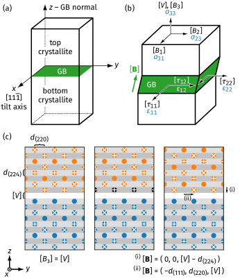
Figure 2: Geometry and excess properties of the bicrystals. (a) The convention used for the coordinate system. (b) The two crystallites are translated with regard to each other by a vector $[\mathbf{B}]$, which is specific to a GB phase. Due to the boundary conditions (lengths in $x$ and $y$ direction are fixed by the bulk phase and the system is free to expand in $z$ direction [9]), excess stresses $[\tau_{11}]$, $[\tau_{22}]$, and $[\tau_{12}]$ occur, while the microscopic translations of the top crystallite lead to the excess volume $[V]$ and the excess shears $[B_{1}]$ and $[B_{2}]$. These excess properties couple to externally applied stresses $\sigma_{31}$, $\sigma_{23}$, $\sigma_{33}$ and strains $\varepsilon_{11}$, $\varepsilon_{22}$, $\varepsilon_{12}$ (blue text). (c) While the components $[B_{1}]$ and $[B_{2}]$ are simple displacements, $[B_{3}]$ consists of both the excess volume $[V]$ and accounts for the shift by full crystallographic planes normal to the GB. Here, this is illustrated for a hypothetical $\Sigma 3$ $[11\overline{1}]$ GB. Different markers indicate the three different $(11\overline{1})$ planes and gray areas the interplanar distance $d_{(224)}$. The left side only has the $[V]$ component. (i) Removing a $\{112\}$ plane (black atoms in the middle), then leads to a shift downwards by $d_{(224)}$ (right side). (ii) This shift can alternatively be expressed by another shift that only changes the $[B_{1}]$ and $[B_{2}]$ components. The latter is always true in our GBs.

II.3 Excess free energy

In the present work, we are interested in the stability of GB phases and GB phase transitions. In pure materials, such phase transitions can occur under externally applied stress or strain, or with changing temperature. The GB phase transitions can be predicted by computing the GB excess free energies of the different GB phases, which we define here as [8, 9]

$$\gamma=[U]-T[S]-\sigma_{33}[V]-\sum_{i=1,2}[B_{i}]\sigma_{3i},$$ (4)

where $[U]$ is the excess internal energy, $[S]$ the excess entropy, $\sigma_{ij}$ the externally applied stress tensor, and $[V]$ the excess volume. Here, $[B_{1}]$ and $[B_{2}]$ are excess shears, which are equal to the microscopic, translational degrees of freedom when no macroscopic stresses or strains are applied [Fig. 2(b)]. The excess volume $[V]$ is not necessarily equal to $[B_{3}]$ as defined here [see Fig. 2(c)], but only $[V]$ enters the free energy. In contrast to Refs. [8, 9], we relax the formality of the bracket notation for notational simplicity, intending them only as indicators of GB excess values. We define all of them as intrinsic values by normalizing $[U]$, $[S]$, and $[V]$ by the GB area. More details and definitions of the excess properties are provided later in Sec. III.2. The free energy at $T=$0\text{\,}\mathrm{K}$$ under applied stresses and strains can be obtained directly in molecular statics by applying the given stress to the system and computing $[U]$, $[V]$, and $[B_{i}]$.

The influence of temperature, however, cannot be calculated directly, because the entropy is not accessible via simple molecular statics or MD simulations. Since we are dealing with pure systems, the entropy is a vibrational entropy and can be computed either via thermodynamic integration [74, 66, 75] or with the quasi-harmonic approximation (QHA) [76, 75]. Here, we chose the latter method for reasons of computational efficiency. Force constant matrices were computed with the dynamical_matrix command in lammps, from which we then obtained the phononic eigenfrequencies in real space. The free energy $F$ was approximated by negelecting quantum-mechanical effects as

$$F=k_{B}T\sum_{i=1}^{3N-3}\ln\frac{h\nu_{i}}{k_{B}T},$$ (5)

where $\nu_{i}$ are the phononic eigenfrequencies excluding the three zero-valued eigenvalues. This describes the systems modeled by MD, which are Newtonian systems, but we found that including quantum-mechanical effects (mostly zero-point vibrations and Debye-like thermal expansion at low temperatures) barely influences the GB free energies, especially at room temperature and above [29]. The GB excess free energy was calculated by subtracting the free energy of a defect-free fcc slab containing the same surfaces and number of atoms as the sample with the GB. Raw data is available in the companion dataset [58].

II.4 Corroborative MD simulations

In addition to calculating $\gamma(\sigma_{ij},T)$, we also verified some example cases using MD simulations at elevated temperature, with and without applied stress and strain. We used systems roughly of size $6\times 16\times$20\text{\,}\mathrm{n}\mathrm{m}^{3}$$ (10 unit cells in tilt axis direction) and a time integration step of $1\text{\,}\mathrm{f}\mathrm{s}$. Temperature was controlled with a Nosé–Hoover thermostat. We typically ran the simulations for up to $40\text{\,}\mathrm{n}\mathrm{s}$, or until the expected GB phase transition could be observed. Raw data is available in the companion dataset [58].

For calculations probing the influence of the temperature or the stress $\sigma_{33}$ normal to the GB, we used open boundaries in $y$ and $z$ direction, while using periodic boundaries in the tilt axis direction ($x$). A barostat at $0\text{\,}\mathrm{P}\mathrm{a}$ was applied in the periodic direction.

For the influence of a tension or compression in $y$ direction ($\varepsilon_{22}$), we kept the $y$ direction periodic and instead introduced open boundaries in the $x$ and $z$ directions. Strain was applied in the periodic direction after scaling the system to the appropriate lattice constant for the target temperature and simulation cell length was subsequently kept constant in the periodic direction.

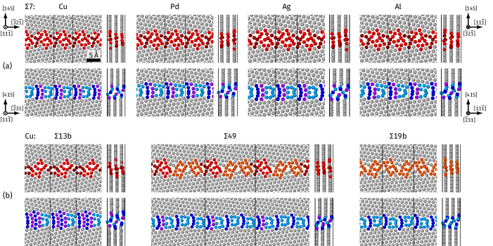
Figure 3: (a) GB phases of $\Sigma$7 tilt GBs in a selection of fcc metals. The top row shows the domino phase (red colors), the bottom row the pearl phase (blue colors). The scale bar is valid for all images and the axes indicate the crystal directions of the top and bottom crystallites, respectively. The axes on the left are for the top views, the axes on the right for the side views. The coloring serves only to highlight the structural motifs. (b) Different misorientations for copper GBs. The axes are equivalent to (a)—for the exact crystal directions see Table 3. Snapshots of the GB structures for all metals and misorientations can be found in Supplemental Figs. Universality of grain boundary phases in fcc metals: Case study on high-angle [111] symmetric tilt grain boundaries–Universality of grain boundary phases in fcc metals: Case study on high-angle [111] symmetric tilt grain boundaries.

II.5 Experimental sample preparation and STEM imaging

In order to verify the simulations, we also experimentally investigated the atomic structure of a near-$\Sigma 49$ GB in copper in addition to the already published experimental structures [28, 29, 47].

For this, a Cu thin film was deposited from a high purity (99.999%) Cu target on (0001)-oriented sapphire substrate by magnetron sputtering. The deposition was performed at room temperature with a radio frequency power supply at $250\text{\,}\mathrm{W}$, a background pressure of $0.66\text{\,}\mathrm{P}\mathrm{a}$, and $20\text{\,}\mathrm{s}\mathrm{c}\mathrm{c}\mathrm{m}$ Ar flow. We obtained a nominal film thickness of $600\text{\,}\mathrm{n}\mathrm{m}$ with a deposition time of $45\text{\,}\mathrm{m}\mathrm{i}\mathrm{n}$. The film was then annealed at $400\text{\,}\mathrm{\SIUnitSymbolCelsius}$ for $2\text{\,}\mathrm{h}$ within the sputtering vacuum chamber.

We identified pure tilt high-angle grain boundaries using electron backscattered diffraction imaging in a Zeiss Auriga scanning electron microscope. In the next step, we lifted out a $\Sigma$49 $\langle 111\rangle$ GB using a Thermo Fisher Scientific Scios2HiVac dual-beam secondary electron microscope equipped with a Ga⁺ focused ion beam (FIB). A plane-view sample was extracted and attached to a Cu grid. For the lamella thinning, an initial current of $0.1\text{\,}\mathrm{n}\mathrm{A}$ and voltage of $30\text{\,}\mathrm{k}\mathrm{V}$ was used, reduced sequentially to $7.7\text{\,}\mathrm{p}\mathrm{A}$ and $5\text{\,}\mathrm{k}\mathrm{V}$. The FIB sample was then transferred to a probe-corrected Thermo Fisher Scientific FEI Titan Themis 80-300 (scanning) transmission electron microscope. A high-brightness field emission gun at an accelerating voltage of $300\text{\,}\mathrm{k}\mathrm{V}$, semi-convergence angle of $17\text{\,}\mathrm{m}\mathrm{r}\mathrm{a}\mathrm{d}$, and probe current of $85\text{\,}\mathrm{p}\mathrm{A}$ was used for imaging. The image was recorded with a high-angle annular dark field (HAADF) detector (Fishione Instruments, Model 3000) with a collection angle of 78 to $200\text{\,}\mathrm{m}\mathrm{r}\mathrm{a}\mathrm{d}$. An image of 50 frames with $1024\times$1024\text{\,}\mathrm{p}\mathrm{x}^{2}$$ with a dwell time of $2\text{\,}\mathrm{\SIUnitSymbolMicro}\mathrm{s}$ and a step size of $12.45\text{\,}\mathrm{p}\mathrm{m}$ was registered and overlaid using the drift compensated frame integration (DCFI) method. The final image was optimized using second order polynomial background correction, Butterworth, and Gaussian filters. The misorientation between both grains was measured from the angles between $\{220\}$ lattice planes of both grains, using an average of at least ten different measurements.

III Structures in different fcc metals

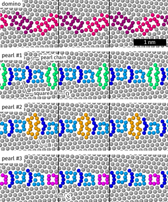
Figure 4: Snapshots of the domino phase and the three variants of the pearl phase in $\Sigma$37c. Here, the material is copper. The three pearl variants differ in their motifs. In addition to the typical squares and pearl chains, which are the same in all variants, we observe variations that we denominate with a letter: either an $\Omega$ motif (pearl #1, green), a B motif (pearl #2, orange), or an $\mathcal{S}$ motif (pearl #3, pink) occurs. At $T=$0\text{\,}\mathrm{K}$$, the lowest-energy pearl variants are pearl #1 for Cu, Ag, and Au; as well as pearl #3 for Ni, Pd, Al, and Pb. The energies of pearl #1 and pearl #2 are typically very similar, except for Pb, where the pearl #2 structure is mechanically unstable.

We performed a computational structure search with Ni, Cu, Pd, Ag, Au, Al, and Pb (M)EAM potentials for the GBs in Table 3. We found that the possible structural motifs are similar not only across different metals [Fig. 3(a) and Supplemental Fig. Universality of grain boundary phases in fcc metals: Case study on high-angle [111] symmetric tilt grain boundaries], but as well across different misorientations from $27.80\mathrm{°}$ to $50.57\mathrm{°}$ [Fig. 3(b) and Supplemental Figs. Universality of grain boundary phases in fcc metals: Case study on high-angle [111] symmetric tilt grain boundaries–Universality of grain boundary phases in fcc metals: Case study on high-angle [111] symmetric tilt grain boundaries]. Indeed, almost all of these motifs resemble the “pearl” and “domino” structures found previously in copper [28, 29]. In some cases, additional structures were found, which will be discussed later.

Viewed from the $[11\overline{1}]$ tilt axis direction, the domino phases consist of pairs of squares (light red motifs in Fig. 3), which are distorted and arranged differently depending on the misorientation. From the side, the $(11\overline{1})$ planes are approximately aligned, with offsets much smaller than the interplanar spacing.

The pearl phases consist of a single square (light blue motifs in Fig. 3) separated by varying amounts of pearl chains (dark blue or purple) when viewed from the $[11\overline{1}]$ tilt axis direction. The $(11\overline{1})$ planes are shifted by approximately half the interplanar spacing, in contrast to the domino phases. Whereas the atomic structure of the domino phase seems to be independent of the material [Fig. 3(a), upper row], slight changes can be observed in the pearl phase [Fig. 3(a), lower row]. In the $\Sigma$7 GBs, two different pearl variants exist, which can be seen by comparing, e.g., Cu and Ag. The variant which occurs in Ag [Fig. 3(a)] and Pb (Supplemental Fig. Universality of grain boundary phases in fcc metals: Case study on high-angle [111] symmetric tilt grain boundaries) appears mirror symmetric in the projection (called aligned pearl from here on), while the variant in the other metals appears asymmetric (called sheared pearl from here on). This minor difference can best be seen by inspecting the light blue square motifs. Furthermore, additional motifs occur in the pearl phase of the $\Sigma$37c GB (Fig. 4 and Ref. [29]), leading to three distinct pearl variants (pearl #1, #2, and #3). Which of these variants has the lowest energy depends on the material, as discussed later.

For the $\Sigma 13$b and $\Sigma 7$ boundaries, some additional low-energy structures occur, which we simply name A, B, and C (shown in Fig. 5). These look different from the pearl and domino phases on visual inspection and are therefore listed separately. We only consider structures that are thermodynamically stable under some condition for at least one element and will later provide a more quantitative analysis of the GB phases, but will otherwise only discuss them where relevant. The A phase of the $\Sigma$13b GB occurs in all metals except Au and Pb, but only has a low energy compared to other GB phases in Al. In the $\Sigma$7 tilt GBs, Pb has the B phase and the C phase is a higher-energy phase in all metals.

Due to the varying quality of empirical potentials—especially in the case of GB structures which have not been included in the fitting database for the respective potential—an independent validation based on experiment or ab initio methods is desirable. Unfortunately, the unit cells of the high $\Sigma$ GBs are too big to allow the required high-accuracy density-functional theory (DFT) simulations, especially when one needs to avoid GB/surface elastic interactions by including a sufficient amount of bulk material. In tests we found that, e.g., the excess volume is very sensitive to such effects. We thus limit ourselves here to a comparison to STEM images obtained for Cu and Al. For Cu $\Sigma$19b and $\Sigma$37c, see Refs. [28, 29]. For these GBs in Al, only the domino phase has been found to date [47]. Additionally, Fig. 6 shows an experimental STEM image of a $\Sigma 49$ pearl phase in copper. All of the structures in the experiments listed above agree well with the simulated structures. Because of the similarity of motifs across misorientations and materials, we are confident that these structure predictions are therefore quite reliable.

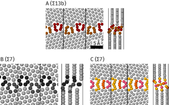
Figure 5: Snapshots of the A, B, and C phases. The material is copper for the A and C phases. The B phase only exists in lead. Snapshots for all materials are provided in Supplemental Figs. Universality of grain boundary phases in fcc metals: Case study on high-angle [111] symmetric tilt grain boundaries and Universality of grain boundary phases in fcc metals: Case study on high-angle [111] symmetric tilt grain boundaries.

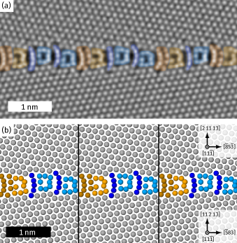
Figure 6: Comparison between a STEM image of a pearl structure in the $\Sigma$49 tilt GB in copper with simulations. (a) HAADF-STEM image of a $\Sigma 49$ tilt GB (misorientation $$$\pm$$$). Note that there is a defect (disconnection) on the right side of the image, where only one blue square is located in between the yellow motifs and where the rightmost yellow motif is mirrored. An image of a longer stretch of the GB can be found in Supplemental Fig. Universality of grain boundary phases in fcc metals: Case study on high-angle [111] symmetric tilt grain boundaries. (b) It can be seen that the structure from the MD simulation is the same. The colors in these images highlight that the $\Sigma 49$ GB consists of alternating motifs from the $\Sigma 7$ GB (yellow) and the $\Sigma 19$b GB (blue).

We note that the structures of the $[11\overline{1}]$ tilt GBs are relatively complex compared to, for example, the more typical kite structures in other (tilt) GBs [30, 38, 21]. Nevertheless, visual inspection already indicates that—except for the special case of the B phase in Pb—material-specific GB structures do not exist and that the presented GB phases are universal in fcc metals. This raises the question of how big the role of the physics and chemistry of a specific material is and how much of that material-specific information needs to be included in a model to reproduce them. We will investigate this in the next section and then proceed to a more quantitative comparison of the GB phases in terms of excess properties.

III.1 Geometry or material physics?

As a first test, we used a Lennard-Jones pair potential as a simplified, generalized model of a densely-packed metal. Physically, pair potentials cannot reproduce the concept of bond order, i.e., the strength of any interatomic bond simply depends on the bond length and not on the atomic environment (such as for example coordination number). By repeating the structure search with this pair potential, we can nevertheless find the same structural motifs in the GBs (see Fig. 7 for the $\Sigma$7 pearl phase).

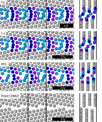
Figure 7: Visual comparison of the $\Sigma$7 pearl structure modeled using the copper EAM potential (Cu), a Lennard-Jones pair potential (L-J), and a next-neighbor pair potential (PP1). For comparison, the data from Frost et al. (1982) [77] (rigid displacement of hard spheres) was also reproduced here, but does not exhibit any of the pearl or domino structures. The scale bar for the model potentials is given in reduced units of the equilibrium fcc bond length $r_{0}$. The axes are the same as in Fig. 3(a).

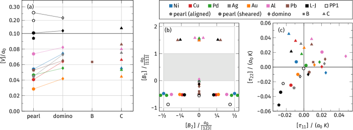
Figure 8: Excess properties of the $\Sigma$7 GBs. Colors of data points correspond to the material, shapes to the GB phase. (a) The normalized excess volumes of all relevant GB phases are shown. The connecting lines highlight the difference in excess volume between the lowest-energy pearl phase and the domino phase and reveal that the domino phases typically have higher excess volumes. Note that the upper part of the graph uses a different scale in order to be able to better discern the data from (M)EAM models. (b) The microscopic, translational degrees of freedom $[\mathbf{B}]$ of the $\Sigma$7 phases. The gray box shows the DSC unit cell, whose repetition is indicated by gray lines. The data are presented such that $[B_{3}]=[V]$ in order to show the data unambiguously. Data points lie outside of the projected DSC unit cell, because this unit cell is triclinic: To move the data points inside the unit cell, DSC vectors with an out-of-plane component are required, such that $[B_{3}]\neq[V]$ (see Supplemental Fig. Universality of grain boundary phases in fcc metals: Case study on high-angle [111] symmetric tilt grain boundaries for more details and different visualizations of this). (c) Two components of the excess GB stress normalized by lattice constant and bulk modulus. The general trend of tensile excess stresses for domino and compressive excess stresses for pearl can be seen. The C phase is distributed around $[\tau_{11}]=0$ with tensile excess stresses in $[\tau_{22}]$. Data for all GBs are provided in Supplemental Figs. Universality of grain boundary phases in fcc metals: Case study on high-angle [111] symmetric tilt grain boundaries–Universality of grain boundary phases in fcc metals: Case study on high-angle [111] symmetric tilt grain boundaries.

In the past, hypothetical GB structures have also been constructed using the assumption of hard spheres due to the lack of realistic interatomic potentials [77]. We used our next-neighbor pair potential to explore how realistic the results are under the assumption of very short-ranged interactions. For this, we took the set of all distinct GB structures obtained using all the other potentials and reminimized them with the next-neighbor potential. While both energy minimization using the next-neighbor pair potential and rigid displacement of hard spheres (as performed by Frost et al. [77]) lead to quite open GB structures, the former are at least able to reproduce some of the motifs produced by longer-ranged potentials (Fig. 7). The two bonds drawn in Fig. 7 are longer with the next-neighbor pair potential than with the Cu and Lennard-Jones potentials. This indicates that longer-ranged interactions and the resulting local bond relaxations are crucial to describe GB structures well. The more realistic, medium-ranged potentials predict an offset between $(11\overline{1})$ planes. A look at the side view of the structure modeled with the next-neighbor pair potential reveals that there is almost no such offset. The hard sphere model interestingly predicts the offset but not the other structural motifs. This is not necessarily the case for all misorientations, but the example of the $\Sigma$7 tilt GB highlights that neither assumptions of next-neighbor interactions nor of hard spheres will be sufficient to capture complex GB structures and their excess properties.

We can conclude here that the GB phases are the result of the fcc geometry and medium-ranged interatomic interactions, but that the GB motifs are still densely packed, otherwise the Lennard-Jones potential would not be able to model them. This purely visual inspection is limited, however, which is why we will continue with an examination of the excess properties for a more quantitative analysis.

III.2 Excess properties

A good definition of separate GB phases is that the corresponding atomic structures have distinct excess properties. If the excess properties are very close in value, we would rather define the structures as defective or as microstates of a GB phase [24, 28, 29, 78]. Furthermore, the excess properties influence the GB thermodynamics (Eq. 4) and are therefore important quantities. We will thus now discuss the individual excess properties introduced in Sec. II.3 in detail for our GB phases.

Figure 8(a) shows the normalized excess volumes $[V]/a_{0}$ of all $\Sigma$7 GB structures [data for other GBs are shown in Supplemental Figs. Universality of grain boundary phases in fcc metals: Case study on high-angle [111] symmetric tilt grain boundaries(a)–Universality of grain boundary phases in fcc metals: Case study on high-angle [111] symmetric tilt grain boundaries(a)] with

$$[V]=\frac{V_{\text{GB}}-N\Omega}{A_{\text{GB}}},$$ (6)

where $V_{\text{GB}}$ is the volume of a region of the simulation cell containing a GB (but no surfaces), $N$ is the number of atoms in that region, $\Omega$ is the atomic volume in a defect-free fcc phase, and $A_{\text{GB}}$ is the area of the GB. The normalization by the fcc lattice constant $a_{0}$ at $T=$0\text{\,}\mathrm{K}$$ makes these volumes unitless and comparable between materials.

In general, domino phases have higher excess volume than pearl phases as indicated by the lines in Fig. 8(a). This trend is reproduced by the Lennard-Jones potential, but not by the next-neighbor pair potential. As already visible in the snapshots and as generally expected, this indicates that the relaxation inside the GB is influenced by several neighbor shells.

Figure 8(b) shows the microscopic, translational degrees of freedom $[\mathbf{B}]$ of the $\Sigma 7$ GB, which are the relative rigid-body displacements between the two crystallites (data for other GBs are shown in Supplemental Figs. Universality of grain boundary phases in fcc metals: Case study on high-angle [111] symmetric tilt grain boundaries–Universality of grain boundary phases in fcc metals: Case study on high-angle [111] symmetric tilt grain boundaries and an illustration of the concept can be found in Fig. 2). $[\mathbf{B}]=0$ represents the case when coincidence sites in the dichromatic pattern actually overlap (which is how the dichromatic pattern is typically plotted), while $[\mathbf{B}]\neq 0$ means that no coincidence sites exist in the dichromatic pattern, i.e., $-[\mathbf{B}]$ represents the shift required to obtain coincidence sites (see also Supplemental Fig. Universality of grain boundary phases in fcc metals: Case study on high-angle [111] symmetric tilt grain boundaries). Due to this, $[\mathbf{B}]$ vectors are equivalent if they can be obtained by adding or subtracting DSC vectors. The components $[B_{1}]$ and $[B_{2}]$ are also called excess shears and enter the GB excess free energy by coupling to externally applied shear stresses (Eq. 4). Due to the symmetry of the present bicrystals with symmetric tilt GBs, $[B_{2}]$ and $-[B_{2}]$ are degenerate states of the same GB phases. This is not the case for $[B_{1}]$, where $-[B_{1}]$ corresponds to switching the top and bottom crystallite.

A typical feature of the pearl phases is that the $(11\overline{1})$ planes of the abutting crystallites are not aligned, but shifted by approximately a half-plane in tilt-axis direction. This is described by $[B_{1}]$. All pearl variants are united by this half-plane shift. The domino phases, in contrast, are characterized by $[B_{1}]\approx 0$. The shift $[B_{2}]$ parallel to the GB plane has two different behaviors in the case of the $\Sigma 7$ GB. Both domino (diamond symbols) and the aligned pearl variant (pentagon symbol) have a fixed value, while the sheared pearl (circles) has material-dependent values, i.e., exhibits some excess shear. The difference in this shift describes the amount of shear that the pearl motifs undergo. An aligned pearl variant was thus found in Ag and Pb in the $\Sigma 7$ GBs, and universally in the $\Sigma 19$b GBs. The $\Sigma 13$b pearl phases are mostly aligned, except for a small asymmetry in Ag, Pb, and the Lennard-Jones model, which we do not indentify as a separate pearl variant. For $\Sigma 49$ and $\Sigma 37$c, only sheared pearl variants exist.

Figure 8(c) and Supplemental Figs. Universality of grain boundary phases in fcc metals: Case study on high-angle [111] symmetric tilt grain boundaries(f)–Universality of grain boundary phases in fcc metals: Case study on high-angle [111] symmetric tilt grain boundaries(f) show the normalized excess GB stresses $[\tau_{ij}]/(a_{0}K)$ with

$$[\tau_{ij}]=\frac{\sigma_{ij}^{\text{GB}}V_{\text{GB}}}{A_{\text{GB}}},$$ (7)

where $\sigma_{ij}^{\text{GB}}$ corresponds to the average of the relevant stress tensor component in the region containing the GB. This definition allows the easy calculation of strain energy via $\int\!A_{\text{GB}}[\tau_{ij}]\mathrm{d}\varepsilon$ (cf. Eq. 10), meaning that the excess stresses are expressed in $\mathrm{J}\mathrm{/}\mathrm{m}^{2}$. Here, the $[\tau_{11}]$ excess stress acts along the tilt axis and $[\tau_{22}]$ along its orthogonal direction within the GB plane [see also Fig. 2(b)]. The normalization by the ground-state fcc lattice constant $a_{0}$ and the bulk modulus $K$ makes these stresses unitless and comparable between materials.

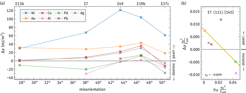
Figure 9: Ground state GB energy difference $\Delta\gamma=\gamma_{0}^{\text{domino}}-\gamma_{0}^{\text{pearl}}$. Positive values mean pearl is stable, negative values that domino is stable. These values are for $T=$0\text{\,}\mathrm{K}$$ and the difference between the lowest-energy pearl variant and the lowest-energy domino variant is used. For $\Sigma$13b, Al is omitted and for $\Sigma$7 Pb is omitted. This is due to other low-energy phases occuring that cannot be classified unambiguously as domino or pearl. (a) GB energy difference as a function of misorientation. The lines are guides for the eye. (b) Correlation between the normalized stacking-fault energy $\gamma_{\text{SF}}$ and $\Delta\gamma$. The normalization ensures that the plotted values are unitless and comparable between different materials. The line represents a linear regression of the data points and the Pearson correlation coefficient $r_{p}$ is reported. More data and the same plot without normalization is provided in Supplemental Fig Universality of grain boundary phases in fcc metals: Case study on high-angle [111] symmetric tilt grain boundaries.

There is a tendency for $[\tau_{11}]<0$ and $[\tau_{22}]<0$ for pearl and $[\tau_{11}]>0$ and $[\tau_{22}]>0$ for domino. Similar trends are observed in all GBs. That means that the pearl phase with lower excess volume is under compression in the in-plane directions of the GB, while the domino phase with higher excess volume is under tension. However, there are several exceptions, such as Al, where the GBs generally tend more towards tensile stresses. The next-neighbor pair potential is once again unable to capture this trend. We will therefore not discuss it any further. The excess stresses of the pearl variants for $\Sigma$37c GBs are very similar within the same material, with the exception of Al [see Supplemental Fig. Universality of grain boundary phases in fcc metals: Case study on high-angle [111] symmetric tilt grain boundaries(f)], indicating again that they are closely related.

Supplemental Figs. Universality of grain boundary phases in fcc metals: Case study on high-angle [111] symmetric tilt grain boundaries–Universality of grain boundary phases in fcc metals: Case study on high-angle [111] symmetric tilt grain boundaries show that the A, B, and C phases are characterized by a $[B_{1}]$ offset of half an interplanar spacing (similar to pearl), but positive $[\tau_{22}]$ (similar to domino), which is why we label them as individual GB phases. We make the distinction between A and B/C because they appear at different CSL boundaries, and differentiate B and C in Pb by their different values of excess shear $[B_{2}]$ and excess stress $[\tau_{22}]$.

IV Thermodynamic stability

IV.1 Ground state stability

For each of the investigated tilt GBs we showed that at least two GB phases (domino and pearl) exist. In order to evaluate which of these GB phases will actually occur, we have to investigate their thermodynamics. We first consider the case of $T=$0\text{\,}\mathrm{K}$$ and no externally applied stress or strain. Here, the ground state GB free energy is

$$\gamma_{0}=[U]=\frac{E_{\text{GB}}-NE_{0}^{\text{fcc}}}{A_{\text{GB}}},$$ (8)

where $E_{\text{GB}}$ is the potential energy of a region of the simulation cell containing a GB (but no surfaces), $N$ is the number of atoms in that region, $E_{0}^{\text{fcc}}$ is the ground-state energy per atom of the defect-free fcc phase, and $A_{\text{GB}}$ is the area of the GB. Note that the internal energy is equal to the potential energy in this section, because we simulate a classical, Newtonian system at zero temperature, i.e., with zero kinetic energy. All GB energies are plotted in Supplemental Fig. Universality of grain boundary phases in fcc metals: Case study on high-angle [111] symmetric tilt grain boundaries.

Figure 9(a) and Supplemental Fig. Universality of grain boundary phases in fcc metals: Case study on high-angle [111] symmetric tilt grain boundaries show the energy difference $\Delta\gamma=\gamma_{0}^{\text{domino}}-\gamma_{0}^{\text{pearl}}$ at $T=$0\text{\,}\mathrm{K}$$ between the domino and pearl phases. In many cases, the pearl phase is stable, with the highest energy difference being observed for the $\Sigma 19$b GB, except for Ni (highest energy difference for $\Sigma 49$). The $\Sigma 19$b GB often also has the lowest overall GB energy, although for Pd, Al, and Pb the $\Sigma 7$ GB has a lower energy (Supplemental Fig. Universality of grain boundary phases in fcc metals: Case study on high-angle [111] symmetric tilt grain boundaries). The domino phase is stable in the $\Sigma 37$c GB in many materials, and seems to also become more favorable again towards lower misorientation angles. Apart from domino and pearl, the A, B, and C phases are usually high-energy GB phases. Exceptions are the A phase in Al, which is quite close in GB energy to the pearl phase, and the B phase in Pb, which is the lowest-energy GB phase in $\Sigma 7$. The C phase only plays a role at higher temperatures, as discussed later in Sec. IV.3.

The Lennard-Jones potential, in contradiction to the more realistic (M)EAM potentials, always predicts that the domino phase is stable [Supplemental Fig. Universality of grain boundary phases in fcc metals: Case study on high-angle [111] symmetric tilt grain boundaries(a)]. This indicates that the Lennard-Jones potential is not a good “generalized” model for most metals: While it is able to capture structural motifs and their excess properties qualitatively, the material-specific physics play a bigger role in the relative thermodynamic stability of the GB phases. This is also important for the evaluation of early simulation work on GB structures [42]: The present results suggest that it is likely that such simulations predicted the wrong ground state because they used pair potentials instead of more realistic material models.

For the (M)EAM potentials, we tried to find a simple predictor of the relative GB phase stability as a function of the material properties, and focus here on the stacking-fault energy $\gamma_{\text{SF}}$. This is a tempting quantity, because both GBs and stacking faults are planar defects and because $\gamma_{\text{SF}}$ is indirectly related to the energy of coherent twin GBs. If we normalize both the stacking-fault energy of the metal and the GB energy difference $\Delta\gamma$ between domino and pearl by the respective fcc lattice constant and cohesive energy, we find that low stacking-fault energies tend to be associated with a preference for the pearl phase and high stacking-fault energies with a preference for the domino phase [Fig. 9(b) and Supplemental Fig. Universality of grain boundary phases in fcc metals: Case study on high-angle [111] symmetric tilt grain boundaries]. This trend is not very convincing, however, since for example nickel deviates quite strongly from the correlation. The data for the $\Sigma 13$b and $\Sigma 37$c GBs is also quite scattered, exhibiting a tendency for an increased stability of domino. A further relation between stacking-fault energy and structure is that the high stacking-fault-energy metals Ni, Pd, and Al have lower energies for the pearl #3 variant in $\Sigma 37$c, while the low stacking-fault-energy metals Cu, Ag and Au (as well as the Lennard-Jones potential) favor pearl #1 or #2. Yet, this relation is undermined by Pb, whose stacking-fault energy is low, but whose ground-state pearl variant is #3. Other material properties have even weaker or no correlation with $\Delta\gamma$.

Ultimately, the relative energies of GB phases have to be computed with sophisticated models (such as EAM potentials or DFT) and simple rules based on bulk properties will be incomplete. This is especially true since the GB energy differences are often small and on the order of $10\text{\,}\mathrm{m}\mathrm{J}\mathrm{/}\mathrm{m}^{2}$, although they can be as high as approximately $120\text{\,}\mathrm{m}\mathrm{J}\mathrm{/}\mathrm{m}^{2}$ [Fig. 9(a)].

IV.2 Stress-dependence of the free energy

Figure 10: GB free energies as a function of an applied stress $\sigma_{33}$ normal to the GB for some selected GBs. (a) In copper $\Sigma 7$ GBs, the domino phase becomes stable under tension. (b) The Al potential also predicts that pearl becomes stable under very high compressive stresses. Furthermore, it exhibits some changes of the curvature of $\gamma$ for the pearl phase, which are associated with small rearrangements of the atomic motifs, leading to the prediction that pearl can additionally become stable at very high tensile stresses. This is likely due to the Al potential being described by cubic splines (the change of curvature representing a transition to another polynomial in the spline). Other potentials do not show such behavior, suggesting that this is most likely an unwanted and unphysical feature of the potential at high stresses/strains. (c) The Pd $\Sigma 49$ GB represents an interesting case due to the low stresses required to transition between pearl and domino. Data for all GBs is available in Supplemental Figs. Universality of grain boundary phases in fcc metals: Case study on high-angle [111] symmetric tilt grain boundaries–Universality of grain boundary phases in fcc metals: Case study on high-angle [111] symmetric tilt grain boundaries.

Figure 11: GB free energies as a function of an applied strain $\varepsilon_{22}$. (a) The domino phase in the $\Sigma$7 GB in Cu can be stabilized under compression. (b) In Al, domino remains stable independent of the applied strain. This is due to both GB phases having positive excess stresses of similar magnitude, meaning that their excess free energy change due to strain is comparable. (c) In the $\Sigma 19$b GB, however, the excess stresses of domino and pearl in Al have opposite signs and a phase transition is possible. The gaps in the curve represent points at which the atoms slightly rearrange within the domino motifs, leading to small jumps in the excess free energy. Data for all GBs is available in Supplemental Figs. Universality of grain boundary phases in fcc metals: Case study on high-angle [111] symmetric tilt grain boundaries–Universality of grain boundary phases in fcc metals: Case study on high-angle [111] symmetric tilt grain boundaries.

The excess free energy at $T=$0\text{\,}\mathrm{K}$$ under applied stresses $\sigma_{33}$, $\sigma_{23}$, and $\sigma_{31}$ can be described as [9]

$$\gamma=[U]-\sigma_{33}[V]-\sum_{i=1,2}[B_{i}]\sigma_{3i}$$ (9)

in the case of tilt GBs [see Fig. 2(b) for a sketch of the stresses and strains]. The excess free energy under applied strain $\varepsilon_{22}$ can be calculated by integrating the work done by the excess stress [9] as

$$\gamma=\gamma_{0}\frac{A_{0}}{A_{\text{GB}}}+\frac{1}{A_{\text{GB}}}\int_{0}^{\varepsilon_{22}}A_{\text{GB}}(\varepsilon)\,[\tau_{22}](\varepsilon)\,\mathrm{d}\varepsilon,$$ (10)

where $A_{0}$ is the GB area before deformation. The calculation for $\varepsilon_{11}$ and $\varepsilon_{12}$ is equivalent. Because the additional work is converted fully into excess internal energy, we can simply express the GB free energy as

$$\gamma=[U],$$ (11)

without need for the integration.

Because the domino phase universally has a higher excess volume than the pearl phase [Fig. 8(a)], it stands to reason that it can be stabilized by a tensile stress $\sigma_{33}$ normal to the GB, while the pearl phase can be stabilized by a compressive stress. Figure 10 and Supplemental Figs. Universality of grain boundary phases in fcc metals: Case study on high-angle [111] symmetric tilt grain boundaries–Universality of grain boundary phases in fcc metals: Case study on high-angle [111] symmetric tilt grain boundaries show that this is the case, but that the required stresses are usually very high (on the order of gigapascals) and sometimes exceed the range of values that were investigated. One interesting exception is for example the Pd $\Sigma$49 GB [Fig. 10(c)], where the ground state energy difference between the domino and pearl phases is close to zero. We thus validated this case by MD simulations at $T=$900\text{\,}\mathrm{K}$$ and $\sigma_{33}=\pm$1\text{\,}\mathrm{G}\mathrm{P}\mathrm{a}$$, starting once from a pearl phase and once from a domino phase. In less than $8\text{\,}\mathrm{n}\mathrm{s}$, the systems under compression transitioned to the pearl phase and the systems under tension to the domino phase, as expected (see Supplemental Fig. Universality of grain boundary phases in fcc metals: Case study on high-angle [111] symmetric tilt grain boundaries).

Another interesting excess property is the excess stress $[\tau_{22}]$ in the GB plane, since it indicates if the GB phase is under compression or tension. Since typically $[\tau_{22}]<0$ for pearl and $[\tau_{22}]>0$ for domino, it seems reasonable that a compressive $\varepsilon_{22}$ would favor domino, while tension would favor pearl (see Eq. 10). Figure 11 and Supplemental Figs. Universality of grain boundary phases in fcc metals: Case study on high-angle [111] symmetric tilt grain boundaries–Universality of grain boundary phases in fcc metals: Case study on high-angle [111] symmetric tilt grain boundaries show that this is indeed a general trend. Exceptions are some GBs in Ni, Al, and Pb. For those GBs, however, the value of $[\tau_{22}]$ is positive for the pearl phase, suppressing a clear trend for a GB phase transition under applied strain. For $\Sigma 13$b GBs in Cu, Ag, or Pb; $\Sigma 7$ Gbs in Cu or Ag; $\Sigma 49$ GBs in Pd or Al; $\Sigma 19$b GBs in Al; and $\Sigma 37$c GBs in Cu or Ag, the required strains for the GB phase transitions are relatively low and could reasonably be observed experimentally (Supplemental Figs. Universality of grain boundary phases in fcc metals: Case study on high-angle [111] symmetric tilt grain boundaries–Universality of grain boundary phases in fcc metals: Case study on high-angle [111] symmetric tilt grain boundaries). We tested this by performing MD simulations for the $\Sigma 7$ GB in Cu with $\varepsilon_{22}=-2\%,+1\%$. We ran the simulations at $T=$900\text{\,}\mathrm{K}$$ in order to accelerate the transition kinetics. A GB phase transition can be observed after less than $4\text{\,}\mathrm{n}\mathrm{s}$, obtaining the domino phase under compression and the pearl phase under tension (Supplemental Fig. Universality of grain boundary phases in fcc metals: Case study on high-angle [111] symmetric tilt grain boundaries).

In addition to externally applied stresses, the rigid-body displacements between the two crystallites could also be determined by restrictions on GB sliding in polycrystals or by the bonding to a substrate in the thin film case [78]. Then, however, $[\mathbf{B}]$ in Eq. 9 no longer corresponds to the displacement, but the excess displacement over the defect-free crystal subject to the same stress $\sigma_{3i}$ [8, 9]. Thus, knowledge of the resulting, system-size-dependent stress state would be required to be able to calculate the free energy, necessitating mesoscale modeling.

Finally, we found that the A, B, and C phases are not stable, except for the A phase in Al, which becomes stable under compression normal to the GB plane or under tensile $\varepsilon_{22}$, and the B phase in Pb, which is the lowest-energy GB phase in $\Sigma 7$ even without applied stress or strain.

In summary, our simulations show that the GB phase transitions both under stress and under strain can be well predicted by the excess properties in the ground state. The GBs thus obey Le Chatelier’s principle and counteract the applied stresses and strains via GB phase transitions.

IV.3 Temperature-dependence of the free energy

The excess free energy without applied stresses or strains is

$$\gamma=[U]-T[S]$$ (12)

for finite temperatures. Note that for $T>$0\text{\,}\mathrm{K}$$, the potential energies $E$ in Eq. 8 have to be replaced by $\langle E\rangle$, which are the average total energies at the given temperature. The excess entropy $[S]$ is not easily accessible to MD simulations. The change of excess free energy $\gamma(T)=\gamma_{0}+\Delta\gamma(T)$ can instead be calculated using either thermodynamic integration [74, 66, 75] or from the phonon eigenfrequencies using the QHA [76, 75]. We chose the latter due to the lower computational demands. In previous works, both methods were found to give equal results [75, 29].

Figure 12: GB free energies as a function of temperature for some selected $\Sigma 7$ GBs. (a) In copper, the pearl phase is stable, until the high-energy, high-temperature C phase becomes stable at around $650\text{\,}\mathrm{K}$. (b) In Al, domino transitions to pearl at around $400\text{\,}\mathrm{K}$, (c) while in Pd the domino phase remains stable at all temperatures. In the latter cases, the C phase is always metastable. The noise in the data is a result of numerical issues with the interatomic potentials, see Appendix A. Data for all GBs is available in Supplemental Figs. Universality of grain boundary phases in fcc metals: Case study on high-angle [111] symmetric tilt grain boundaries–Universality of grain boundary phases in fcc metals: Case study on high-angle [111] symmetric tilt grain boundaries.

In most cases, the pearl phase remains stable over the whole temperature range (Fig. 12 and Supplemental Figs. Universality of grain boundary phases in fcc metals: Case study on high-angle [111] symmetric tilt grain boundaries–Universality of grain boundary phases in fcc metals: Case study on high-angle [111] symmetric tilt grain boundaries). If the domino phase is stable at low temperatures ($\Sigma$13b: Pd, Al; $\Sigma 7$: Pd, Al; $\Sigma$49: Al; $\Sigma 37$c: Cu, Pd, Ag, Al, Pb) it usually transforms to pearl at higher temperatures, except for $\Sigma$7 Pd (domino is always stable). In $\Sigma 13$b Pb, as well as $\Sigma 19$b Ag and Pb, pearl transforms to domino at higher temperatures. In $\Sigma 49$ Pd, both phases have approximately equal free energy. Some limited experimental data is available for copper (Refs. [28, 29] and Fig. 6) and supports the modeling. In Al, only the domino phase has been found to date [47]. That contradicts the data obtained with the Al potential for the $\Sigma 19$b GB (but not the others). The predicted energy differences between domino and pearl are small, however, which complicates the comparison to experiment: Either the relative stability of the GB phases is predicted incorrectly by the potential or small residual strains in the experiments, which were performed on thin films, could potentially destabilize the pearl phase.

The only non-domino/non-pearl phases that become stable with increasing temperature are the A phase in Al $\Sigma 13$b GBs and the C phase in Cu and Ag $\Sigma 7$ GBs (Fig. 12 and Supplemental Figs. Universality of grain boundary phases in fcc metals: Case study on high-angle [111] symmetric tilt grain boundaries and Universality of grain boundary phases in fcc metals: Case study on high-angle [111] symmetric tilt grain boundaries). In general, the investigated GBs mostly exhibit domino and pearl phases, with A, B, and C being the exceptions.

In order to furthermore exclude the existence of additional GB phases and to validate the QHA calculations, we ran MD simulations for up to $40\text{\,}\mathrm{n}\mathrm{s}$ with the GBs in contact with open boundaries at elevated temperatures [21] for some example cases. We chose high temperatures to enable GB phase transitions on MD timescales. No additional GB phases were discovered. For the $\Sigma 7$ GBs, we found that Ni ($T=$1300\text{\,}\mathrm{K}$$) and Al ($T=$900\text{\,}\mathrm{K}$$) transition to the pearl phase at high temperatures independent on the starting structure, as expected (Supplemental Figs. Universality of grain boundary phases in fcc metals: Case study on high-angle [111] symmetric tilt grain boundaries and Universality of grain boundary phases in fcc metals: Case study on high-angle [111] symmetric tilt grain boundaries). The Al sample contained many defects after the heat treatment. Both Cu ($T=$1100\text{\,}\mathrm{K}$$) and Ag ($T=$1100\text{\,}\mathrm{K}$$) quickly transitioned to the pearl phase if starting from domino and slowly nucleated the C phase, also as expected (Supplemental Figs. Universality of grain boundary phases in fcc metals: Case study on high-angle [111] symmetric tilt grain boundaries and Universality of grain boundary phases in fcc metals: Case study on high-angle [111] symmetric tilt grain boundaries). In the latter case, however, C and pearl phases often appear to coexist, hinting that the C phase is some variant of the pearl phase. The only case that could not confirm the QHA calculations was the Pd $\Sigma 7$ GB: neither systems containing pearl, nor containing domino would undergo phase transitions when heated to $900\text{\,}\mathrm{K}$ (Supplemental Fig. Universality of grain boundary phases in fcc metals: Case study on high-angle [111] symmetric tilt grain boundaries). This is likely due to the small free energy differences between the GB phases and possibly a result of the low mobility of the phase junction between the two GB phases [28]. Apart from the $\Sigma 7$ GBs, we also annealed a Ni $\Sigma 37$c GB at $1000\text{\,}\mathrm{K}$ (Supplemental Fig. Universality of grain boundary phases in fcc metals: Case study on high-angle [111] symmetric tilt grain boundaries). The QHA calculations predict that the pearl #3 variant is stable at low temperatures and pearl #1 and #2 at high temperatures, the latter GB phases having almost equal free energies [Supplemental Fig. Universality of grain boundary phases in fcc metals: Case study on high-angle [111] symmetric tilt grain boundaries(a)]. We could indeed observe this transition between pearl variants, although the result at high temperature still contained several pearl #3 motifs. This is not surprising, since these structures should most likely be treated as microstates of a pearl GB phase [29].

Due to the rough tendency of pearl being stable at higher temperatures, it is tempting to treat the pearl structure as a high-entropy GB phase. But while it is universal that domino has higher excess volumes and thus couples to $\sigma_{33}$, a higher entropy of the pearl phase cannot be observed in the majority of cases. When pearl is stable over the whole temperature range, the slope of $\gamma(T)$ is often similar for pearl and domino, indicating approximately equal excess entropies. In pure materials, the excess entropy is vibrational and results from the GB phonon modes. This means that the GB vibrations are therefore quite material dependent.

IV.4 Latent heat and order of the GB phase transition

Figure 13: Order of the GB phase transition for the Al $\Sigma 7$ GB. The solid lines indicate the stable GB phase. (a) In equilibrium, the domino phase is stable at low temperatures, while the pearl phase is stable above $T\approx$406\text{\,}\mathrm{K}$$. (b) This results in a discontinuity of the entropy, resulting in a latent heat of $\Delta[H]=$31.5\text{\,}\mathrm{m}\mathrm{J}\mathrm{/}\mathrm{m}^{2}$$. This value approximately corresponds to the difference in ground state GB energies $\gamma_{0}^{\text{pearl}}-\gamma_{0}^{\text{domino}}=$30.8\text{\,}\mathrm{m}\mathrm{J}\mathrm{/}\mathrm{m}^{2}$$.

Finally, we will shortly discuss the order of the GB phase transition. According to the Ehrenfest classification, first order phase transitions are those that have a discontinuity in the first derivative of the relevant thermodynamic potential. Alternatively, first order phase transitions have a latent heat. In bulk materials, these definitions are virtually equivalent and the latent heat is the difference in enthalpy $\Delta H=\Delta G+T\Delta S$ of the phases, with $G$ being the Gibbs free energy and $S$ the entropy. By definition, it is $\Delta G=0$ at the transition point $T_{t}$, allowing us to write $\Delta H=T_{t}\Delta S$. The entropy of the system in equilibrium is discontinuous at $T_{t}$ for $\Delta S\neq 0$ due to the change from one phase to another with different entropy. This means that the phase transition is also of the first order according to Ehrenfest because the entropy of a phase is the first derivative of the free energy ($S=-\partial G/\partial T$) at constant pressure. Equation 12 with $\Delta\gamma=0$ leads to a similar result for GBs, namely $\Delta[H]=\Delta[U]=T_{t}\Delta[S]$ for $\sigma_{3i}=0$ (no work is done by the system on its surroundings without externally applied stresses, only heat is exchanged). The excess entropy can be calculated as

$$[S]=-\frac{\mathrm{d}\gamma}{\mathrm{d}T}+\sum_{i,j=1,2}\bigl{(}[\tau_{ij}]-\delta_{ij}\gamma\bigr{)}\frac{\mathrm{d}\varepsilon_{ij}}{\mathrm{d}T},$$ (13)

(see Eq. 14 of Ref. [9], noting that we already normalize $[S]$ by the GB area) where the strains $\varepsilon_{ij}$ correspond to the thermal expansion of the grains, which result in work being done by the grain boundary against the expansion, even without externally applied stress. (Note that this work term does not come into play when defining the latent heat as $\Delta[H]=\Delta[U]$, because the phase transformation takes place at constant $T=T_{t}$ and thus constant $\varepsilon_{ij}$. It is only required to calculate $[S]$.) For cubic systems, we can replace $\mathrm{d}\varepsilon_{ij}/\mathrm{d}T$ with the isotropic thermal expansion coefficient $\alpha_{T}$ and simplify to

$$[S]=-\frac{\mathrm{d}\gamma}{\mathrm{d}T}+\alpha_{T}\bigl{(}[\tau_{11}]+[\tau_{22}]-2\gamma\bigr{)}.$$ (14)

We ignore the weak temperature dependence of the excess stresses in further calculations. Figure 13 shows an example for the $\Sigma 7$ GB in Al. At the transition temperature of around $405\text{\,}\mathrm{K}$, the excess free energy of the system in equilibrium changes slope and the entropy is discontinuous, resulting in a finite latent heat. Equivalent results would be obtained for the other GB phase transitions. The GB phase transitions in this work are thus first order phase transitions.

V Summary and conclusion

Simulations using (M)EAM potentials reveal that a range of high-angle, symmetric $[11\overline{1}]$ tilt GBs in fcc metals exhibit mainly two GB phases, here called domino and pearl. We found that the domino and pearl phases, respectively, have comparable structures and thermodynamic excess properties across different $\Sigma$ boundaries with misorientations from $27.8\mathrm{°}$ to $50.6\mathrm{°}$ and for all of the seven investigated fcc metals. Indeed, the structures seem universal enough to be modeled using simple pair potentials, although medium-range interatomic interactions are required to recover the trends of the excess properties. The thermodynamic stability as a function of stress, strain, or temperature, however, is more specific to the material:

• In many cases the pearl phases are stable at $T=$0\text{\,}\mathrm{K}$$ and if they are not, they often become stable at higher temperatures due to their higher excess entropy. This is not universal however, suggesting that the GB vibrations are material dependent.

• There does not seem to be a clear predictor of which GB phase is the ground state, although there is some weak correlation with the stacking-fault energy, with low stacking-fault energy favoring pearl.

• The domino phases have higher excess volumes in almost all cases, meaning that they are stabilized by tension applied normal to the GB, while the pearl phases are stabilized under compression.

• The pearl phases tend to exhibit negative excess stresses in the GB plane ($[\tau_{11}]$ and $[\tau_{22}]$), while the domino phases exhibit positive excess stresses. This predicts their thermodynamic stability quite well: compression in the GB plane stabilizes domino, while tension stabilizes pearl, opposite to the previous case of stress applied normal to the GB.

• The required stresses for GB phase transformation can exceeed $5\text{\,}\mathrm{G}\mathrm{P}\mathrm{a}$ and would be unlikely to occur in real materials. In some cases, however, stresses below $1\text{\,}\mathrm{G}\mathrm{P}\mathrm{a}$ or even close to zero, as well as strains below 1%, are sufficient. We confirmed some of the latter cases with MD simulations.

While there are always some exceptions to the above rules, the present results suggest that GB structures and phases discovered for one material are likely generalizable to a whole class of materials (in this case fcc metals). It remains to be seen if that is a feature of densely-packed metals or if it is also true in, e.g., covalently or ionically bonded materials. The addition of alloying elements is also likely to lead to more material-specific GB thermodynamics.

Appendix A Numerical issues of the interatomic potentials

The calculation of free energies in the QHA depends on the force constant matrix, which is closely related to the Hessian of the potential energy. This requires that the interatomic potential is smooth up to the second derivative, otherwise the resulting free energy is noisy. In MD simulations, only first derivatives of the potential energy are used and any noise is averaged out due to the natural thermal fluctuations of the dynamic simulation, making numerical issues with the potential unnoticeable. In the present work, we found that the Pd, Au, and Al potentials result in noisy free energy data in our QHA calculations.

For Al, this is not due to the formalism of the potential, but a consequence of limited precision of the tabulated potential data in the file distributed via the NIST Interatomic Potentials Repository [55]. In lammps, EAM potentials are tabulated—typically with dense sampling of data points—in text files and interpolated during simulation. In current numerical simulations, floating point numbers are usually represented using the IEEE 754 double-precision format, which corresponds to a precision of at least 15 significant digits in decimal representation. The text files used to produce the Al potential file contain fewer significant digits. We tested the potential by using the $\Sigma 19$b domino GB phase and isotropically straining the simulation cell, while recording the potential energy (Supplemental Fig. Universality of grain boundary phases in fcc metals: Case study on high-angle [111] symmetric tilt grain boundaries). Taking numerical derivatives of the potential energy, we obtain smooth curves up to the first derivative, but see noise from the second derivative on. This is not surprising, since numerical derivatives are particularly sensitive, even to small noise. We then recovered the original nodal points, reproduced the potential, and constructed a tabulated EAM potential file with full machine precision (see companion dataset [58] for details and the potential file). This leads to smooth results up to the third derivative of the potential energy (Supplemental Fig. Universality of grain boundary phases in fcc metals: Case study on high-angle [111] symmetric tilt grain boundaries) while preserving the properties of the potential (we verified this for the bulk properties listed in Table 2, as well as the excess properties of the GB phases).

Additionally, the construction of the Al potential from cubic splines leads to changes of curvature of the GB free energy [visible for example in Fig. 10(b) at high stresses or in Fig. 12(b) at around $550\text{\,}\mathrm{K}$]. This indicates a shortcoming of the fitting with cubic splines to a limited reference database. It seems that the flexibility of representing the EAM functions with splines would require more strained reference data points in order to correctly model highly strained systems.

For Pd and Au, the first and second derivatives of the potential energy are sufficiently smooth (Supplemental Fig. Universality of grain boundary phases in fcc metals: Case study on high-angle [111] symmetric tilt grain boundaries). The problem comes from the cutoff function in these cases. It appears that the cutoff functions are relatively abrupt. This works well for the defect-free crystalline structures, where interatomic distances are usually smaller or larger than the cutoff distance. In the case of our GBs, however, bond lengths around the cutoff distance can appear and certain bond lengths can cross this distance during thermal or mechanical straining. As depicted in Supplemental Fig. Universality of grain boundary phases in fcc metals: Case study on high-angle [111] symmetric tilt grain boundaries, this can lead to discontinuities in the forces and thus jumps and/or noise in the second derivatives. It is nontrivial to improve the existing potentials without changing their properties and we therefore use the unchanged potentials here.

References

- Priester [2013] L. Priester, Grain Boundaries: From Theory to Engineering (Springer, Berlin, Germany, 2013).
- Frolov and Mishin [2015] T. Frolov and Y. Mishin, Phases, phase equilibria, and phase rules in low-dimensional systems, J. Chem. Phys. 143, 044706 (2015).
- Tang et al. [2006] M. Tang, W. C. Carter, and R. M. Cannon, Diffuse interface model for structural transitions of grain boundaries, Phys. Rev. B 73, 024102 (2006).
- Dillon et al. [2007] S. J. Dillon, M. Tang, W. C. Carter, and M. P. Harmer, Complexion: A new concept for kinetic engineering in materials science, Acta Mater. 55, 6208 (2007).
- Cantwell et al. [2014] P. R. Cantwell, M. Tang, S. J. Dillon, J. Luo, G. S. Rohrer, and M. P. Harmer, Grain boundary complexions, Acta Mater. 62, 1 (2014).
- Cantwell et al. [2020] P. R. Cantwell, T. Frolov, T. J. Rupert, A. R. Krause, C. J. Marvel, G. S. Rohrer, J. M. Rickman, and M. P. Harmer, Grain boundary complexion transitions, Annu. Rev. Mater. Res. 50, 465 (2020).
- Gibbs [1948] J. W. Gibbs, The Collected Works of J. Willard Gibbs, Volume 1: Thermodynamics (Yale University Press, New Haven, CT, USA, 1948).
- Frolov and Mishin [2012a] T. Frolov and Y. Mishin, Thermodynamics of coherent interfaces under mechanical stresses. I. Theory, Phys. Rev. B 85, 224106 (2012a).
- Frolov and Mishin [2012b] T. Frolov and Y. Mishin, Thermodynamics of coherent interfaces under mechanical stresses. II. Application to atomistic simulation of grain boundaries, Phys. Rev. B 85, 224107 (2012b).
- Kaplan et al. [2013] W. D. Kaplan, D. Chatain, P. Wynblatt, and W. C. Carter, A review of wetting versus adsorption, complexions, and related phenomena: the rosetta stone of wetting, J. Mater. Sci. 48, 5681 (2013).
- Hart [1968] E. W. Hart, Two-dimensional phase transformation in grain boundaries, Scr. Metall. 2, 179 (1968).
- Cahn [1982] W. Cahn, J., Transitions and phase equilibria among grain boundary structures, J. Phys. Colloques 43, C6 (1982).
- Rottman [1988] C. Rottman, Theory of phase transitions at internal interfaces, J. Phys. Colloques 49, C5 (1988).
- Ference and Balluffi [1988] T. G. Ference and R. W. Balluffi, Observation of a reversible grain boundary faceting transition induced by changes of composition, Scr. Metall. 22, 1929 (1988).
- Sigle et al. [2002] W. Sigle, L.-S. Ciiang, and W. Gusr, On the correlation between grain-boundary segregation, faceting and embrittlement in Bi-doped Cu, Philos. Mag. A 82, 1595 (2002).
- Frolov et al. [2015] T. Frolov, M. Asta, and Y. Mishin, Segregation-induced phase transformations in grain boundaries, Phys. Rev. B 92, 020103 (2015).
- Khalajhedayati and Rupert [2015] A. Khalajhedayati and T. J. Rupert, High-temperature stability and grain boundary complexion formation in a nanocrystalline Cu–Zr alloy, JOM 67, 2788 (2015).
- Pan and Rupert [2016] Z. Pan and T. J. Rupert, Effect of grain boundary character on segregation-induced structural transitions, Phys. Rev. B 93, 134113 (2016).
- Peter et al. [2018] N. J. Peter, T. Frolov, M. J. Duarte, R. Hadian, C. Ophus, C. Kirchlechner, C. H. Liebscher, and G. Dehm, Segregation-induced nanofaceting transition at an asymmetric tilt grain boundary in copper, Phys. Rev. Lett. 121, 255502 (2018).
- Wu et al. [2009] Z. X. Wu, Y. W. Zhang, and D. J. Srolovitz, Grain boundary finite length faceting, Acta Mater. 57, 4278 (2009).
- Frolov et al. [2013a] T. Frolov, D. L. Olmsted, M. Asta, and Y. Mishin, Structural phase transformations in metallic grain boundaries, Nat. Commun. 4, 1899 (2013a).
- Hickman and Mishin [2017] J. Hickman and Y. Mishin, Extra variable in grain boundary description, Phys. Rev. Mater. 1, 010601 (2017).
- Aramfard and Deng [2018] M. Aramfard and C. Deng, Mechanically enhanced grain boundary structural phase transformation in Cu, Acta Mater. 146, 304 (2018).
- Zhu et al. [2018] Q. Zhu, A. Samanta, B. Li, R. E. Rudd, and T. Frolov, Predicting phase behavior of grain boundaries with evolutionary search and machine learning, Nat. Commun. 9, 467 (2018).
- Frolov et al. [2018a] T. Frolov, W. Setyawan, R. J. Kurtz, J. Marian, A. R. Oganov, R. E. Rudd, and Q. Zhu, Grain boundary phases in bcc metals, Nanoscale 10, 8253 (2018a).
- Frolov et al. [2018b] T. Frolov, Q. Zhu, T. Oppelstrup, J. Marian, and R. E. Rudd, Structures and transitions in bcc tungsten grain boundaries and their role in the absorption of point defects, Acta Mater. 159, 123 (2018b).
- Yang et al. [2020] C. Yang, M. Zhang, and L. Qi, Grain boundary structure search by using an evolutionary algorithm with effective mutation methods, Comput. Mater. Sci. 184, 109812 (2020).
- Meiners et al. [2020a] T. Meiners, T. Frolov, R. E. Rudd, G. Dehm, and C. H. Liebscher, Observations of grain-boundary phase transformations in an elemental metal, Nature 579, 375 (2020a).
- Frommeyer et al. [2022] L. Frommeyer, T. Brink, R. Freitas, T. Frolov, G. Dehm, and C. H. Liebscher, Dual phase patterning during a congruent grain boundary phase transition in elemental copper, Nat. Commun. 13, 3331 (2022).
- Mills et al. [1992] M. J. Mills, M. S. Daw, G. J. Thomas, and F. Cosandey, High-resolution transmission electron microscopy of grain boundaries in aluminum and correlation with atomistic calculations, Ultramicroscopy 40, 247 (1992).
- Mills [1993] M. J. Mills, High resolution transmission electron microscopy and atomistic calculations of grain boundaries in metals and intermetallics, Mater. Sci. Eng. A 166, 35 (1993).
- Rabkin et al. [1999] E. Rabkin, C. Minkwitz, C. Herzig, and L. Klinger, Evidence for structural multiplicity of the = 3 incoherent twin boundary in Cu from grain-boundary diffusion measurements, Philos. Mag. Lett. 79, 409 (1999).
- Divinski et al. [2012] S. V. Divinski, H. Edelhoff, and S. Prokofjev, Diffusion and segregation of silver in copper 5(310) grain boundary, Phys. Rev. B 85, 144104 (2012).
- Frolov et al. [2013b] T. Frolov, S. V. Divinski, M. Asta, and Y. Mishin, Effect of interface phase transformations on diffusion and segregation in high-angle grain boundaries, Phys. Rev. Lett. 110, 255502 (2013b).
- Rajeshwari K. et al. [2020] S. Rajeshwari K., S. Sankaran, K. C. Hari Kumar, H. Rösner, M. Peterlechner, V. A. Esin, S. Divinski, and G. Wilde, Grain boundary diffusion and grain boundary structures of a Ni–Cr–Fe-alloy: Evidences for grain boundary phase transitions, Acta Mater. 195, 501 (2020).
- Frolov [2014] T. Frolov, Effect of interfacial structural phase transitions on the coupled motion of grain boundaries: A molecular dynamics study, Appl. Phys. Lett. 104, 211905 (2014).
- Wei et al. [2021] J. Wei, B. Feng, R. Ishikawa, T. Yokoi, K. Matsunaga, N. Shibata, and Y. Ikuhara, Direct imaging of atomistic grain boundary migration, Nat. Mater. 20, 951 (2021).
- Luo et al. [2011] J. Luo, H. Cheng, K. M. Asl, C. J. Kiely, and M. P. Harmer, The role of a bilayer interfacial phase on liquid metal embrittlement, Science 333, 1730 (2011).
- Pan and Rupert [2015] Z. Pan and T. J. Rupert, Amorphous intergranular films as toughening structural features, Acta Mater. 89, 205 (2015).
- Feng et al. [2018] L. Feng, R. Hao, J. Lambros, and S. J. Dillon, The influence of dopants and complexion transitions on grain boundary fracture in alumina, Acta Mater. 142, 121 (2018).
- Bishara et al. [2021] H. Bishara, S. Lee, T. Brink, M. Ghidelli, and G. Dehm, Understanding grain boundary electrical resistivity in Cu: The effect of boundary structure, ACS Nano 15, 16607 (2021).
- Sutton and Vitek [1983a] A. P. Sutton and V. Vitek, On the structure of tilt grain boundaries in cubic metals I. Symmetrical tilt boundaries, Phil. Trans. R. Soc. Lond. A 309, 1 (1983a).
- Bishop and Chalmers [1968] G. H. Bishop and B. Chalmers, A coincidence – ledge – dislocation description of grain boundaries, Scr. Metall. 2, 133 (1968).
- Sutton and Vitek [1983b] A. P. Sutton and V. Vitek, On the structure of tilt grain boundaries in cubic metals II. Asymmetrical tilt boundaries, Phil. Trans. R. Soc. Lond. A 309, 37 (1983b).
- Sutton and Vitek [1983c] A. P. Sutton and V. Vitek, On the structure of tilt grain boundaries in cubic metals III. Generalizations of the structural study and implications for the properties of grain boundaries, Phil. Trans. R. Soc. Lond. A 309, 55 (1983c).
- Han et al. [2017] J. Han, V. Vitek, and D. J. Srolovitz, The grain-boundary structural unit model redux, Acta Mater. 133, 186 (2017).
- Ahmad et al. [2023a] S. Ahmad, T. Brink, C. H. Liebscher, and G. Dehm, Deciphering the atomic structures of [111] tilt GBs as a function of 5 macroscopic parameters in Al by correlating STEM with atomistic simulations, in preparation (2023a).
- Mishin [2004] Y. Mishin, Atomistic modeling of the and -phases of the Ni–Al system, Acta Mater. 52, 1451 (2004).
- Mishin et al. [2001] Y. Mishin, M. J. Mehl, D. A. Papaconstantopoulos, A. F. Voter, and J. D. Kress, Structural stability and lattice defects in copper: Ab initio, tight-binding, and embedded-atom calculations, Phys. Rev. B 63, 224106 (2001).
- Foiles and Hoyt [2001] S. M. Foiles and J. J. Hoyt, Computer Simulation of Bubble Growth in Metals Due to He, techreport SAND2001-0661 (Sandia National Laboratories, 2001).
- Williams et al. [2006] P. L. Williams, Y. Mishin, and J. C. Hamilton, An embedded-atom potential for the Cu–Ag system, Modell. Simul. Mater. Sci. Eng. 14, 817 (2006).
- Foiles et al. [1986] S. M. Foiles, M. I. Baskes, and M. S. Daw, Embedded-atom-method functions for the fcc metals Cu, Ag, Au, Ni, Pd, Pt, and their alloys, Phys. Rev. B 33, 7983 (1986).
- Mishin et al. [1999] Y. Mishin, D. Farkas, M. J. Mehl, and D. A. Papaconstantopoulos, Interatomic potentials for monoatomic metals from experimental data and ab initio calculations, Phys. Rev. B 59, 3393 (1999).
- Lee et al. [2003] B.-J. Lee, J.-H. Shim, and M. I. Baskes, Semiempirical atomic potentials for the fcc metals Cu, Ag, Au, Ni, Pd, Pt, Al, and Pb based on first and second nearest-neighbor modified embedded atom method, Phys. Rev. B 68, 144112 (2003).
- [55] NIST Interatomic Potentials Repository: https://www.ctcms.nist.gov/potentials.
- Plimpton [1995] S. Plimpton, Fast parallel algorithms for short-range molecular dynamics, J. Comp. Phys. 117, 1 (1995), https://lammps.org/.
- Thompson et al. [2022] A. P. Thompson, H. M. Aktulga, R. Berger, D. S. Bolintineanu, W. M. Brown, P. S. Crozier, P. J. in ’t Veld, A. Kohlmeyer, S. G. Moore, T. D. Nguyen, R. Shan, M. J. Stevens, J. Tranchida, C. Trott, and S. J. Plimpton, LAMMPS - a flexible simulation tool for particle-based materials modeling at the atomic, meso, and continuum scales, Comput. Phys. Commun. 271, 108171 (2022), https://lammps.org/.
- Brink et al. [2022] T. Brink, L. Langenohl, H. Bishara, and G. Dehm, Dataset for “Universality of grain boundary phases in fcc metals: Case study on high-angle [111] symmetric tilt grain boundaries”, Zenodo (2022).
- Kittel [2005] C. Kittel, Introduction to Solid State Physics, 8th ed. (Wiley, Hoboken, New Jersey, USA, 2005).
- Rumble [2022] J. Rumble, ed., CRC Handbook of Chemistry and Physics, 103rd ed. (CRC Press, Boca Raton, FL, USA, 2022).
- Ullmaier [1991] H. Ullmaier, ed., Atomic Defects in Metals, Landolt-Börnstein – Group III Condensed Matter, Vol. 25 (Springer, Berlin, Germany, 1991).
- Vitos et al. [1998] L. Vitos, A. V. Ruban, H. L. Skriver, and J. Kollár, The surface energy of metals, Surf. Sci. 411, 186 (1998).
- Bernstein and Tadmor [2004] N. Bernstein and E. B. Tadmor, Tight-binding calculations of stacking energies and twinnability in fcc metals, Phys. Rev. B 69, 094116 (2004).
- Ogata et al. [2002] S. Ogata, J. Li, and S. Yip, Ideal pure shear strength of aluminum and copper, Science 298, 807 (2002).
- Zhu et al. [2021] L.-F. Zhu, J. Janssen, S. Ishibashi, F. Körmann, B. Grabowski, and J. Neugebauer, A fully automated approach to calculate the melting temperature of elemental crystals, Comput. Mater. Sci. 187, 110065 (2021).
- Freitas et al. [2016] R. Freitas, M. Asta, and M. de Koning, Nonequilibrium free-energy calculation of solids using LAMMPS, Comput. Mater. Sci. 112, 333 (2016).
- Stukowski et al. [2010] A. Stukowski, K. Albe, and D. Farkas, Nanotwinned fcc metals: Strengthening versus softening mechanisms, Phys. Rev. B 82, 224103 (2010).
- Stukowski [2010a] A. Stukowski, Atomic-scale modeling of nanostructured metals and alloys, Ph.D. thesis, Technische Universität Darmstadt (2010a).
- Kim et al. [2015] K.-H. Kim, J. B. Jeon, and B.-J. Lee, Modified embedded-atom method interatomic potentials for Mg–X (X=Y, Sn, Ca) binary systems, Calphad 48, 27 (2015).
- Meiners et al. [2020b] T. Meiners, J. M. Duarte, G. Richter, G. Dehm, and C. H. Liebscher, Tantalum and zirconium induced structural transitions at complex [111] tilt grain boundaries in copper, Acta Mater. 190, 93 (2020b).
- Langenohl et al. [2022] L. Langenohl, T. Brink, G. Richter, G. Dehm, and C. H. Liebscher, Atomic resolution observations of silver segregation in a [111] tilt grain boundary in copper, arXiv:2212.01180 [cond-mat.mtrl-sci] (2022).
- [72] See Supplemental Material at [link to be inserted by publisher] for figures containing the data for all GB phases, as well as some additional details on the simulation and analysis methods.
- Stukowski [2010b] A. Stukowski, Visualization and analysis of atomistic simulation data with OVITO – the Open Visualization Tool, Modell. Simul. Mater. Sci. Eng. 18, 015012 (2010b), https://ovito.org/.
- Frenkel and Ladd [1984] D. Frenkel and A. J. C. Ladd, New Monte Carlo method to compute the free energy of arbitrary solids. Application to the fcc and hcp phases of hard spheres, J. Chem. Phys. 81, 3188 (1984).
- Freitas et al. [2018] R. Freitas, R. E. Rudd, M. Asta, and T. Frolov, Free energy of grain boundary phases: Atomistic calculations for grain boundary in Cu, Phys. Rev. Mater. 2, 093603 (2018).
- Foiles [1994] S. M. Foiles, Evaluation of harmonic methods for calculating the free energy of defects in solids, Phys. Rev. B 49, 14930 (1994).
- Frost et al. [1982] H. J. Frost, M. F. Ashby, and F. A. Spaepen, A catalogue of [100], [110], and [111] symmetric tilt boundaries in face-centered cubic hard sphere crystals, Tech. Rep. (Harvard Division of Applied Sciences, 1982).
- Ahmad et al. [2023b] S. Ahmad, T. Brink, C. H. Liebscher, and G. Dehm, Microstates and defects of incoherent 3 [111] twin boundaries in aluminum, Acta Mater. 243, 118499 (2023b).