A Gaussian Process Regression based Dynamical Models Learning Algorithm for Target Tracking

Abstract

Maneuvering target tracking is a challenging problem for sensor systems because of the unpredictability of the targets’ motions. This paper proposes a novel data-driven method for learning the dynamical motion model of a target. Non-parametric Gaussian process regression (GPR) is used to learn a target’s naturally shift invariant motion (NSIM) behavior, which is translationally invariant and does not need to be constantly updated as the target moves. The learned Gaussian processes (GPs) can be applied to track targets within different surveillance regions from the surveillance region of the training data by being incorporated into the particle filter (PF) implementation. The performance of our proposed approach is evaluated over different maneuvering scenarios by being compared with commonly used interacting multiple model (IMM)–PF methods and provides around 90% performance improvement for a multi-target tracking (MTT) highly maneuvering scenario.

I Introduction

Maneuvering target tracking is a fundamental task in sensor-based applications, such as radar, sonar, and navigation [1, 2, 3]. Based on the Bayesian framework, target tracking is usually solved via a recursive update of the posterior probability density function (pdf) of the target states. The application of Bayesian filters is based on dynamical motion models and sensor measurement models [3, 4]. However, there may be significant motion model uncertainty when targets undergo unknown or mixed maneuvering behaviors [5, 6], such that the evolution of the target state is too complex to be approximated by a reasonable number of mathematical models. The uncertainty in motion behavior can also be due to various parameters in generative models not being known a priori or if they are time-varying. The tracking performance of Bayesian filters would degrade and even become unacceptable if incorrect models or parameters are applied. This paper focuses on the issue of learning uncertain motion models with higher flexibility and incorporating the learned models into the Bayesian framework for target tracking.

I-A State-of-the-Art in Bayesian Filters

MM methods are commonly used to deal with the model uncertainty problem [5]. The basic idea of multiple model (MM) methods is to use a bank of elemental filters with different motion models to capture the mixed motion behaviors. Then, the overall estimate is generated based on the results achieved by each elemental filter [5]. For the cases when the target’s behavior is a time-varying or doubly-stochastic process, [6] and [7] incorporated adaptive parameter estimation methods into the Bayesian filter framework to deal with the uncertainty of unknown parameters, where the unknown parameter is estimated by approximating its distribution with particles and corresponding weights. MM methods may be limited in performance if the assumed trajectories are not modeled accurately enough to capture all aspects of the motion behaviors, and the estimation of unknown parameters results in increased computation complexity.

I-B State-of-the-Art in Machine Learning Approaches

As an alternative to traditional Bayesian methods, machine learning-based tracking algorithms have been proposed recently [8, 9, 10, 11, 12, 13, 14]. In [8], a quadruplet convolutional neural network (CNN) based algorithm was designed to learn object association for multi-object tracking via 2D image processing. An extended target tracking method using a Gaussian process (GP) was proposed in [9] and [10] to track the irregularly shaped object whose moving trajectory follows a fixed motion model. These papers use a GP for shape modeling but not for capturing the motion behavior. A long short-term memory (LSTM) neural network was used in [11] to perform the prediction step of target localization. The proposed filter with LSTM prediction can improve the tracking accuracy by using computationally efficient low-dimensional state spaces but only considers the single-target tracking (STT) scenario. In [11], the continuous-discrete estimation of the target’s trajectory is viewed as a one-dimensional sparse GP, with time as the independent variable and measurements acquired at discrete times. Recursive GP-based approaches for target tracking and smoothing were developed in [12, 13], with online training and parameter learning. Only STT with a linear observation model (i.e. $X$-axis and $Y$-axis coordinates) is considered. Furthermore, it was assumed that the motion model could be decomposed into separate models for the X and Y axes. In [14], the motion behavior of a single target is modeled as a Markov process which switches between the constant velocity (CV) and coordinated turn (CT) models with the specified transition probabilities. The complex mixed model is learned as joint GPs for position and velocity prediction. Then the trained GPs are integrated into the PF for tracking the maneuvering targets in real-time.

The learning-based tracking algorithms proposed in [12, 13, 14] were for motion models based on Cartesian positions which are problematic because positions are not translationally invariant, i.e. the motion model needs to be constantly updated as the target moves. This paper proposes learning a naturally shift invariant motion (NSIM) model. Specifically, the change in the target’s Cartesian positions on the $X$-axis and $Y$-axis in one instant (i.e. Cartesian velocities), instead of the Cartesian positions, is learned as multi-independent GPs.

I-C Proposed Method and Contributions

This work follows a learning-to-track framework for tracking problems with uncertain motion models and proposes a new learning method with which the motion behaviors of targets are learned as GPs based on a training data set. Then we show how the learned motion models are integrated into the PF and belief propagation (BP) to realize target tracking. The three main contributions are:

• We propose a new GP-based dynamical motion model learning method. The NSIM behavior of a target is learned using Gaussian process regression (GPR) based on the Cartesian velocities. The learned GPs are translationally invariant and can be applied to track objects within different surveillance regions from the surveillance region of the training data.

• We explore the potential of using the learned motion model within the PF [15, 16] for STT and PF based BP [17, 18, 19] for multi-target tracking (MTT) to demonstrate that the proposed algorithm is a plug-and-play learning method in target tracking systems.

• The proposed learning method is firstly tested in STT with different motion scenarios to demonstrate its capability to learn uncertain motion models with higher flexibility. Then, the learned motion model is plugged into MTT, which shows significant improvement in tracking performance compared with interacting multiple model (IMM)-PF methods. Additionally, offline learning is performed only once and then applied for MTT. Hence, the online tracking time is not affected by the learning process.

Compared with the available learning-based tracking methods using target positions, the motivations and advantages of the proposed GP-based NSIM model include:

• The information available for use in the tracking problems may be limited depending on how we envisage getting the training data. For example, if the data was taken from other previously tracked targets, it could be challenging to access speed or acceleration.

• The existing methods learn the motion models based on target positions, which are not translationally invariant and need to update the model as the target moves constantly. Moreover, the tested targets’ surveillance regions may differ from the training data’s surveillance region. On the other hand, the motion of an object is usually controlled by the application of a force, e.g. aircraft control surfaces. As such, the motion is translationally invariant. Therefore, the proposed NSIM model based on Cartesian velocities will be translationally invariant and can reduce the requirement of training data size and algorithm complexity.

• The learned GP-based NSIM model can provide confidence intervals for particle sampling in the prediction step of the PF to provide a reliable estimate of model uncertainty.

I-D Paper Organization and Notations

The remainder of this paper is organized as follows. The problem solved in this investigation is defined in Section II. Section III reviews the GPR and proposes the GP-based learning method of NSIM behavior. The proposed algorithm, which incorporates the learned GPs into the target tracking, is developed in Section IV. Simulation results and performance comparisons are presented in Section V. Conclusions are provided in Section VI. This paper presents matrices with uppercase letters, vectors with boldface lowercase letters and scalars with lowercase letters. The notations are defined and summarized in Table I.

Table I: The meaning of notations.

Notation	Meaning
$\mathbf{x}^{*}_{1:N}$	Target states of training data sequence
$\mathbf{y}^{*}_{1:N}$	Observations of training data sequence
$\mathbf{x}_{1:T}$	Target states of test data sequence
$\mathbf{y}_{1:T}$	Observations of test data sequence
$n=0,\dots,N-1$	Training time index
$t=1,\dots,T$	Test tracking time index
$k=1,\dots,K$	Target index
$\left[\xi_{t,k},\eta_{t,k}\right]$	Cartesian positions at 2-D plane
$\left[\Delta\xi_{t,k},\Delta\eta_{t,k}\right]$	Cartesian velocities at 2-D plane
$v_{t,k}$	Ground speed
$\phi_{t,k}$	Velocity heading angle
${\alpha}^{t}_{t,k}$	Along-track acceleration
${\alpha}^{n}_{t,k}$	Cross-track acceleration
$Q$	Covariance matrix of process noise
$R$	Covariance matrix of measurement noise
$\mathcal{D}$	Training data set
${f}(\cdot)$	Motion function
$h(\cdot)$	Measurement function
${\dot{f}}^{*\xi}(\cdot)$	$X$-axis velocity motion function for training
${\dot{f}}^{*\eta}(\cdot)$	$Y$-axis velocity motion function for training
${\dot{f}}^{\xi}(\cdot)$	$X$-axis velocity motion function for testing
${\dot{f}}^{\eta}(\cdot)$	$Y$-axis velocity motion function for testing

II Problem Definition and Background

In this section, we will introduce the system model and conventional Bayesian approaches of target tracking.

II-A System Model

The dynamic state-space model (DSSM) for target tracking is given by the following motion and measurement models:

$$\mathbf{x}_{t,k} =f_{k}(\mathbf{x}_{t-1,k},\mathbf{v}_{t-1,k})$$ (1)

$$\mathbf{y}_{t,k} =h_{k}(\mathbf{x}_{t,k},\mathbf{e}_{t,k}).$$ (2)

Here, $t$ represents the time index, $t=1,\dots,T$, $k$ is the target index, $k=1,\dots,K$. For STT scenarios, $K=1$. The state motion model and the measurement model are represented as $f_{k}:\mathbb{R}^{n_{x}}\times\mathbb{R}^{n_{v}}\rightarrow\mathbb{R}^{n_{x}}$ and $h_{k}:\mathbb{R}^{n_{x}}\times\mathbb{R}^{n_{e}}\rightarrow\mathbb{R}^{n_{y}}$, respectively, where $n_{x}$, $n_{v}$, $n_{y}$ and $n_{e}$ are dimensions of the state, process noise, observation, and measurement noise vectors, respectively. The process noise $\mathbf{v}_{t,k}$ and the measurement noise $\mathbf{e}_{t,k}$ are assumed to be additive white Gaussian noise (AWGN). At each time instant, the sensor node detects each target with detection probability $P_{D}\leq 1$. Owing to missed detections and clutter, the number of detected measurements at time $t$ may not be equal to $K$. $\mathcal{K}_{t}$ is defined as the number of measurements at time $t$ and is time-varying. The set of measurements detected at time $t$ is denoted as ${Y}_{t}=\{\mathbf{y}_{t,1},\dots,\mathbf{y}_{t,\mathcal{K}_{t}}\}$. The measurement index is represented as $\kappa$ and $\kappa=1,\dots,\mathcal{K}_{t}$. The number of clutter points is modeled as a Poisson point process with intensity $\lambda_{\mathrm{fa}}$. The corresponding clutter measurements are independent and identically distributed (iid) with pdf $p_{c}(\mathbf{y}_{t,\kappa})$.

II-B Sequential Bayesian Filters for Target Tracking

Based on the Bayesian theorem, most target tracking methods are sequential Bayesian filters which consist of the prediction and the update steps. In the prediction step, the prior distribution of targets’ states at time $t$ is calculated via the Chapman–Kolmogorov equation as [20]

$$\begin{split}&p(\mathbf{x}_{t,1:K}\mid{Y_{1:t-1}})\\ &\qquad=\int{p(\mathbf{x}_{t,1:K}\mid\mathbf{x}_{t-1,1:K})p(\mathbf{x}_{t-1,1:K}\mid{Y_{1:t-1}})}d\mathbf{x}_{t-1,1:K}.\end{split}$$ (3)

In the update step, the joint posterior pdf of the targets’ states is calculated as [20]

$$p(\mathbf{x}_{t,1:K}\mid{Y_{1:t}})=\frac{p(Y_{t}\mid\mathbf{x}_{t,1:K})p(\mathbf{x}_{t,1:K}\mid{Y_{1:t-1}})}{\int p(Y_{t}\mid\mathbf{x}_{t,1:K})p(\mathbf{x}_{t,1:K}\mid{Y_{1:t-1}})d\mathbf{x}_{t,1:K}}.$$ (4)

For STT in non-linear systems, the PF uses random particles with associated weights to approximate the posterior pdf as

$$p(\mathbf{x}_{t}\mid{Y_{1:t}})\approx\sum_{m=1}^{M}w_{n}^{\{m\}}\delta\left(\mathbf{x}_{t}-\mathbf{x}_{t}^{\{m\}}\right)$$ (5)

where $\delta(\cdot)$ is the Dirac delta function, the number of particles used at a given time is represented as $M$. The particles $\mathbf{x}_{t}^{\{1:M\}}$ are drawn from an importance density which can be set as $\mathbf{x}_{t}^{\{m\}}=f(\mathbf{x}_{t-1}^{\{m\}},\mathbf{v}_{t-1}^{\{m\}})$[15].

For MTT, the association between targets and measurements is described by two data association (DA) vectors shown in Fig. 1 [21, 22], i.e. the target-oriented association vector $\mathbf{a}_{t}=\left[{a}_{t,1},\dots,{a}_{t,K}\right]^{\rm{T}}$ and the measurement-oriented association vector $\mathbf{b}_{t}=\left[{b}_{t,1},\dots,{b}_{t,\mathcal{K}_{t}}\right]^{\rm{T}}$ where $\mathcal{K}_{t}$ is the number of measurements at time $t$. The DA vectors are defined as [23]

• ${a}_{t,k}\triangleq\kappa\in\{1,\dots,\mathcal{K}_{t}\}$ if at time $t$, the $k$-th target generates the $\kappa$-th measurement.

• ${a}_{t,k}\triangleq\kappa=0$ if at time $t$, the $k$-th target does not generate a measurement, i.e. missed detection occurs.

• ${b}_{t,\kappa}\triangleq k\in\{1,\dots,K\}$ if at time $t$, the $\kappa$-th measurement is hypothesized to be associated with $k$-th target.

• ${b}_{t,\kappa}\triangleq k=0$ if at time $t$, the $\kappa$-th measurement is hypothesized not to be generated by a target, i.e. clutter.

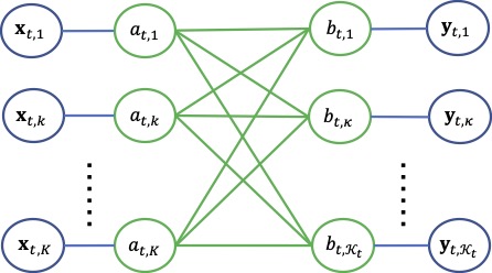
Figure 1: Factor graphs for single-sensor MTT, $\mathbf{a}_{t}=\left[{a}_{t,1},\dots,{a}_{t,K}\right]^{\rm{T}}$ is the target-oriented association vector and $\mathbf{b}_{t}=\left[{b}_{t,1},\dots,{b}_{t,\mathcal{K}_{t}}\right]^{\rm{T}}$ is the measurement-oriented association vector.

The objective of MTT is to calculate the marginal posterior pdf $p(\mathbf{x}_{t,k}\mid Y_{1:t}),\,k=1,\dots,K$ by

$$p(\mathbf{x}_{t,k}\mid Y_{1:t})=\sum_{a_{t,k}=0}^{\mathcal{K}_{t}}p(\mathbf{x}_{t,k}\mid a_{t,k},Y_{1:t})p(a_{t,k}\mid Y_{1:t})$$ (6)

where the marginal association probability, i.e. $p(a_{t,k}\mid Y_{1:t})$, approximates based on the loopy BP algorithm, as given by Eqn. (22) in [21].

It should be noted that most of the existing STT/MTT filters are fully model-driven and, therefore, of use when the DSSM is explicitly available. However, assuming that the state motion function is given as a simple deterministic model is restrictive. These filters are intractable for some applications where the motion model is very complicated. Instead, information about the state transitions can be inferred from examples of preceding states and current states pairs. Hence, we assume that the motion model is learned using the non-parametric Gaussian process regression (GPR) [24]. The measurement model is deterministic by different sensor types with no correlation over time and is in a known parametric form, i.e. we know the acquisition model. In the next section, we will discuss the application of GPR to learn motion behavior.

III Gaussian Progress Regression for Motion Behavior Learning

GP models are widely used to perform Bayesian non-linear regression. A GP model takes a training data set and a kernel as the input and outputs a joint Gaussian distribution that characterizes the value of the function at some given points [25]. One practical advantage of GP is having confidence intervals for predictions that provide a reliable estimate of uncertainty. In this section, we briefly review the standard theory of GPR and then introduce the proposed GP-based method for motion behavior learning.

III-A Gaussian Process Regression

The GP model for regression can be considered as a distribution over a function $g(\mathbf{x})$ and is defined as [9]

$${g}(\mathbf{x}) \sim\mathcal{GP}(\mathbf{m}({\mathbf{x}}),\mathit{k}({\mathbf{x}},{\mathbf{x}}^{\prime}))$$ (7)

where $\mathbf{x}$ and ${\mathbf{x}}^{\prime}$ represent the input variables. The mean function $\mathbf{m}({\mathbf{x}})$ and the covariance function $k({{\mathbf{x}}},{\mathbf{x}}^{\prime})$ of two variables $\mathbf{x}$ and ${\mathbf{x}}^{\prime}$ are defined as [26]

$$\mathbf{m}({\mathbf{x}}) =\mathbb{E}\left[{g}({\mathbf{x}})\right]$$ (8)

$$k({{\mathbf{x}}},{\mathbf{x}}^{\prime}) =\mathbb{E}\left[\left({g}({\mathbf{x}})-{\mathbf{m}}({\mathbf{x}})\right)\left({g}({\mathbf{x}}^{\prime})-\mathbf{m}({\mathbf{x}}^{\prime})\right)\right].$$ (9)

Let us consider a general GPR problem with noisy observations from an unknown function described as

$$z=g(\mathbf{x})+\mathbf{v},\qquad\mathbf{v}\sim\mathcal{N}(0,\sigma^{2}_{v}{I}).$$ (10)

Here, $\sigma^{2}_{v}$ is the variance of the noise. The training data set is denoted as $\mathcal{D}=\{{X}^{*},\mathbf{z}^{*}\}$, where ${X}^{*}=\left[{\mathbf{x}}_{0}^{*},{\mathbf{x}}_{1}^{*},\dots,{\mathbf{x}}_{N-1}^{*}\right]^{\rm{T}}$ are the inputs with the corresponding outputs $\mathbf{z}^{*}=\left[z_{0}^{*},{z}_{1}^{*},\dots,{z}_{N-1}^{*}\right]^{\rm{T}}$. The purpose of GPR is to derive the latent distributions of the vector ${\mathbf{g}}=\left[g(\mathbf{x}_{1}),g(\mathbf{x}_{2}),\dots,g(\mathbf{x}_{T})\right]^{\rm{T}}$ at the test inputs $X=\left[{\mathbf{x}}_{1},{\mathbf{x}}_{2},\dots,{\mathbf{x}}_{T}\right]^{\rm{T}}$, conditioned on the test measurements $\mathbf{z}=\left[{z}_{1},{z}_{2},\dots,z_{T}\right]^{\rm{T}}$ and the training data set $\mathcal{D}$. Specifically, the joint distribution of the training measurements $\mathbf{z}^{*}$ and the function at one test point, i.e. ${g}_{t}\triangleq g({\mathbf{x}}_{t})$, is assumed to be Gaussian and is given by

$$\begin{bmatrix}\mathbf{z}^{*}\\ g_{t}\end{bmatrix}\sim\mathcal{N}\left(\begin{bmatrix}\mathbf{m}(X^{*})\\ {m}({\mathbf{x}}_{t})\end{bmatrix},\begin{bmatrix}K(X^{*},X^{*})+\sigma_{v}^{2}I&\mathbf{k}_{t}(X^{*},{\mathbf{x}}_{t})\\ \mathbf{k}_{t}({\mathbf{x}}_{t},X^{*})&k({\mathbf{x}}_{t},{\mathbf{x}}_{t})\end{bmatrix}\right).$$ (11)

Here, ${\mathbf{k}}_{t}(X^{*},{\mathbf{x}}_{t})=[k({\mathbf{x}}_{0}^{*},{\mathbf{x}}_{t}),\dots,k({\mathbf{x}}^{*}_{N-1},{\mathbf{x}}_{t})]^{\rm{T}}$, $k({\mathbf{x}}_{t},{\mathbf{x}}_{t})$ is the covariance of ${\mathbf{x}}_{t}$, and $K(X^{*},X^{*})$ denotes the covariance matrix for the training input data [14]. The conditional distribution of the function $g(\mathbf{x}_{t})$ is then derived from the joint density in (11) and written as the following standard forms:

$$({g}_{t}|\mathcal{D})\sim\mathcal{N}(\mathbf{m}({g}_{t}),\mathbb{V}\left[{g}_{t}\right])$$ (12a)

$$\mathbf{m}({{g}}_{t})={m}({\mathbf{x}}_{t})+{\mathbf{k}}_{t}^{\mathrm{T}}[K(X^{*},X^{*})+\sigma_{v}^{2}I]^{-1}\left({\mathbf{{z}}}^{*}-\mathbf{m}(X^{*})\right)$$ (12b)

$$\mathbb{V}\left[{g}_{t}\right]=k({\mathbf{x}}_{t},{\mathbf{x}}_{t})-{\mathbf{k}}_{t}^{\mathrm{T}}[K(X^{*},X^{*})+\sigma_{v}^{2}I]^{-1}{{\mathbf{k}}_{t}}$$ (12c)

where ${\mathbf{k}}_{t}$ is the abbreviation for ${\mathbf{k}}(X^{*},{\mathbf{x}}_{t})$. The most widely used kernel function is the squared exponential (SE) covariance function [24], which is also used in this paper,

$$k(\mathbf{x},\mathbf{x}^{\prime})=\sigma_{0}^{2}\exp\left[-\frac{1}{2}\frac{\left(\mathbf{x}-\mathbf{x}^{\prime}\right)^{\rm{T}}\left(\mathbf{x}-\mathbf{x}^{\prime}\right)}{l^{2}}\right].$$ (13)

Here, the hyperparameters $\sigma_{0}^{2}$ and $l$ represent the prior variance of the signal amplitude and the kernel function length scale, respectively.

III-B GP-based Motion Behaviors Learning — Limited Information of Training State

This paper proposes a new GP-based learning method. I.e., the naturally shift invariant motion (NSIM) behavior of a target is learned as GPs based on the Cartesian velocities. The Cartesian positions $\xi_{t,k}$ and $\eta_{t,k}$ are converted into the Cartesian velocities as $\Delta\xi_{t-1,k}=\xi_{t,k}-\xi_{t-1,k}$ and $\Delta\eta_{t-1,k}=\eta_{t,k}-\eta_{t-1,k}$, respectively. The NSIM models, i.e. $\Delta\xi_{k}={\dot{f}}^{\xi}\left(\Delta\mathbf{x}_{t-1,k}\right):\mathbb{R}^{2}\rightarrow\mathbb{R}^{1}$ and $\Delta\eta_{k}={\dot{f}}^{\eta}\left(\Delta\mathbf{x}_{t-1,k}\right):\mathbb{R}^{2}\rightarrow\mathbb{R}^{1}$, are learned as GPs, where $\Delta{\mathbf{x}_{t-1,k}}\triangleq\left[\Delta\xi_{t-1,k},\Delta\eta_{t-1,k}\right]^{\rm{T}}$. As most target maneuvers are coupled across coordinates, the learned models capture the crucial characteristics of the target behavior during maneuvers by using both Cartesian velocities as the input of the GPs. Specifically, the motion behavior of the targets in (1) is rewritten as

$$\Delta\xi_{t,k} ={\dot{f}}^{\xi}\left(\Delta\mathbf{x}_{t-1,k}\right)$$ (14a)

$$\xi_{t+1,k} =\xi_{t,k}+\Delta\xi_{t,k}+{v}_{t,k}^{\xi}$$ (14b)

$$\Delta\eta_{t,k} ={\dot{f}}^{\eta}\left(\Delta\mathbf{x}_{t-1,k}\right)$$ (14c)

$$\eta_{t+1,k} =\eta_{t,k}+\Delta\eta_{t,k}+{v}_{t,k}^{\eta}.$$ (14d)

The proposed GP-based method for prediction shown in Fig. 2 involves offline training and online prediction steps. The training data is used offline to capture the statistical characteristics of the motion behavior of the targets, which are then transferred to online tracking for state prediction.

• Offline training: To train the Cartesian velocity motion functions, we take training data sets $\mathcal{D}_{\xi}:=\{\Delta X^{*},\Delta{\Xi}^{*}\}$ and $\mathcal{D}_{\eta}:=\{\Delta X^{*},\Delta{\Gamma}^{*}\}$. Specifically, the training inputs for both GPs are the same as

  $$\Delta X^{*} =[\Delta{\mathbf{x}}_{0}^{*},\Delta{\mathbf{x}}_{2}^{*},\dots,\Delta{\mathbf{x}}_{N-1}^{*}]$$

  while the output data are different and set as

  $$\Delta{\Xi}^{*} =[\Delta{\xi}_{1}^{*},\Delta{\xi}_{2}^{*},\dots,\Delta{\xi}_{N}^{*}]^{T}$$

  $$\Delta{\Gamma}^{*} =[\Delta{\eta}_{1}^{*},\Delta{\eta}_{2}^{*},\dots,\Delta{\eta}_{N}^{*}]^{T}.$$

  Here, $N$ denotes the number of training samples. The Cartesian $X$/$Y$ velocity motion functions in the offline training process, i.e. $\dot{f}^{*\xi}(\Delta{\mathbf{x}^{*}_{n}})$ and ${\dot{f}}^{*\eta}(\Delta{\mathbf{x}^{*}_{n}})$, are modeled as two GPs shown in (15) and (16).

  $${\dot{f}}^{*\xi}(\Delta{\mathbf{x}^{*}_{n}}) \sim\mathcal{GP}_{\xi}\left({m}_{\xi}(\Delta{\mathbf{x}^{*}_{n}}),k_{\xi}(\Delta{\mathbf{x}^{*}_{n}},(\Delta{\mathbf{x}^{*}_{n}})^{\prime})\right)$$ (15)

  $${\dot{f}}^{*\eta}(\Delta{\mathbf{x}^{*}_{n}}) \sim\mathcal{GP}_{\eta}\left({m}_{\eta}(\Delta{\mathbf{x}^{*}_{n}}),k_{\eta}(\Delta{\mathbf{x}^{*}_{n}},(\Delta{\mathbf{x}^{*}_{n}})^{\prime})\right).$$ (16)

  Here, $\Delta{\mathbf{x}^{*}_{n}}$ and $\Delta{\mathbf{x}^{*}_{n}}^{\prime}$ are the input variables, the squared exponential (SE) defined in (13) are used to calculate $k_{\xi}(\Delta{\mathbf{x}^{*}_{n}},(\Delta{\mathbf{x}^{*}_{n}})^{\prime})$ and $k_{\eta}(\Delta{\mathbf{x}^{*}_{n}},(\Delta{\mathbf{x}^{*}_{n}})^{\prime})$ with the same hyperparameters $\sigma_{0}^{2}$ and $l$. Examples of the learned GPs are shown in Fig. 3, where the motion behavior of the target follows the gradual coordinated turns (GCT) model, defined in Section V. The turn rate of the target follows the left and coordinated right turns ($\pm 15^{\circ}$/s for 10s). In Fig. 3, the $X$ and $Y$ axes represent the input of the GP, i.e., Cartesian velocities, and the Z axis represents the prediction value. The training samples are shown in blue points. The orange-edge and green surfaces represent the mean value of the predictive Gaussian distribution for the $X$-axis and $Y$-axis velocity, respectively, which are joint functions of current Cartesian velocities.

  

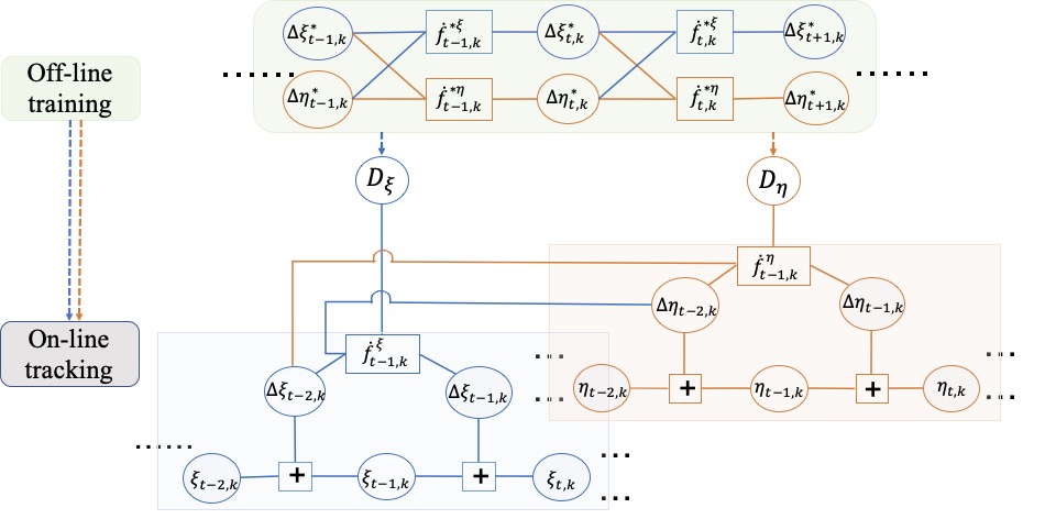
  Figure 2: The factor graph of the proposed GP-based learning algorithm for state prediction mainly includes offline training and online prediction processes. Legend: Circles – variable nodes; Squares – factor nodes. The process for the prediction on $X$-axis is marked in blue. The process for the prediction on $Y$-axis is marked in orange.

• Online Prediction: In the following, we describe the estimation of the $X$-axis position ${\xi}$. The estimation of the $Y$-axis position ${\eta}$ is done similarly and so is not discussed. The estimated parameters at time $t-1$ include the Cartesian position and velocity estimates represented as $\big{\{}\hat{\mathbf{x}}_{t-1,k}=\left[\hat{\xi}_{t-1,k},\hat{\eta}_{t-1,k}\right]^{\rm{T}},\widehat{\Delta\mathbf{x}}_{t-2,k}=\left[\widehat{\Delta\xi}_{t-2,k},\widehat{\Delta\eta}_{t-2,k}\right]^{\rm{T}}\big{\}}$. The predictive distribution of the tracking state ${\xi}_{t,k}$ is partitioned as

  $$p({\xi}_{t,k}\mid\hat{\mathbf{x}}_{t-1,k}\widehat{\Delta\mathbf{x}}_{t-2,k},\mathcal{D}_{\xi})$$ (17)

  $$\qquad=\iint p({\xi}_{t,k}\mid\hat{\xi}_{t-1,k},{\Delta{\xi}}_{t-1,k})$$

  $$\qquad\qquad\times p({\Delta{\xi}}_{t-1,k}\mid\dot{f}_{t-2,k}^{\xi},\mathcal{D}_{\xi})d{\Delta{\xi}}_{t-1,k}d\dot{f}_{t-2,k}^{\xi}.$$

  Here, $\dot{f}_{t-2,k}^{\xi}\triangleq\dot{f}^{\xi}(\widehat{\Delta\mathbf{x}}_{t-2,k})$. The pdfs in (17) are further calculated in (18) – (19),

  $$\begin{split}&p({\xi}_{t,k}\mid\,\hat{\xi}_{t-1,k},{\Delta{\xi}}_{t-1,k})=\mathcal{N}\left({\xi}_{t,k};\,\hat{\xi}_{t-1,k}+\Delta{\xi}_{t-1,k},Q_{\xi}\right)\end{split}$$ (18)

  $$\begin{split}&p({\Delta{\xi}}_{t-1,k}\mid\dot{f}_{t-2,k}^{\xi},\mathcal{D}_{\xi})\\ &\qquad\qquad=\mathcal{N}\left(\Delta{\xi}_{t-1,k};\,\bar{\mu}_{{\xi}}(\widehat{\Delta\mathbf{x}}_{t-2,k}),\bar{K}_{\xi}(\widehat{\Delta\mathbf{x}}_{t-2,k})\right)\end{split}$$ (19)

  where the predictive mean $\bar{\mu}_{{\xi}}(\widehat{\Delta\mathbf{x}}_{t-2,k})$ and covariance $\bar{K}_{\xi}(\widehat{\Delta\mathbf{x}}_{t-2,k})$ are calculated in (20) and (21), respectively.

  $$\bar{\mu}_{\xi}(\widehat{\Delta\mathbf{x}}_{t-2,k})=\bm{k}_{\xi}\left[{K}_{{\xi}}+\sigma_{v}^{2}I\right]^{-1}\Delta{\Xi}^{*}$$ (20)

  $$\bar{K}_{\xi}(\widehat{\Delta\mathbf{x}}_{t-2,k})={k}_{\xi}(\widehat{\Delta\mathbf{x}}_{t-2,k},\widehat{\Delta\mathbf{x}}_{t-2,k})-\bm{k}_{\xi}^{\mathrm{T}}[{K}_{{\xi}}+\sigma_{v}^{2}I]^{-1}{\bm{k}_{\xi}}$$ (21)

  where $\bm{k}_{\xi}$ and ${K}_{{\xi}}$ are the abbreviations for $\bm{k}_{\xi}(\Delta{X}^{*},\widehat{\Delta\mathbf{x}}_{t-2,k})$ and ${K}_{{\xi}}(\Delta{X}^{*},\Delta{X}^{*})$.

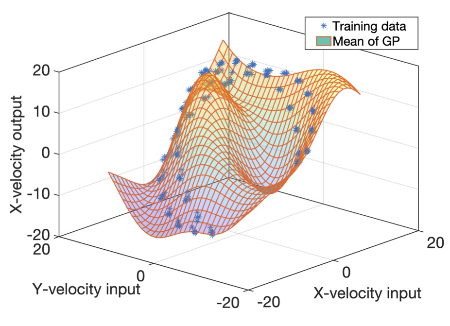
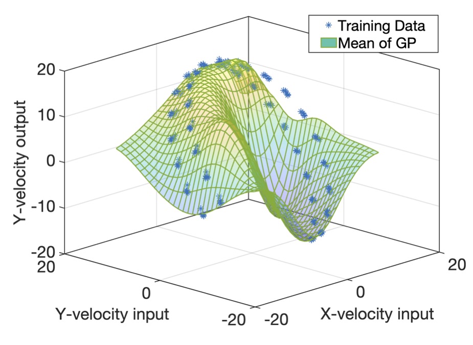
Figure 3: Example of two-dimensional GPR. Legend: Points – training samples; Surface – the mean function of the trained GPs. (a) GP for $X$-axis velocity. (b) GP for $Y$-axis velocity.

IV Incorporation of Learned GP-based NSIM Model into Target Tracking

For nonlinear and non-Gaussian motion and observation models, the pdf of the hidden states in (6) and (17) cannot be evaluated in closed form. Therefore, particle-based implementation algorithms are commonly used for target tracking. The proposed GP-based NSIM model learning method is plugged into the PF and PF-based belief propagation (BP) algorithms in this section. When the parametric motion model is unavailable, particles are drawn based on the learned GPs. The learned GP-based PF-MP implementation for MTT is summarized in Algorithm I. The GP-based PF for STT is implemented the same way without executing Step 5, i.e. the loopy BP. Note that the data association for MTT is obtained by running an iterative BP algorithm following [21]. Therefore, the proposed algorithm is still valid when the target number is unknown and time varying.

Algorithm 1 Learned GP based PF-BP filter

0:  Measurement model $h(\cdot)$ and training data $\mathcal{D}$.

1:  Off-line training: The X/Y-axis velocity motion functions are modeled as two GPs, ${\dot{f}}^{*\xi}(\Delta{\mathbf{x}^{*}_{n}})\sim\mathcal{GP}_{\xi}\left({m}_{\xi}(\Delta{\mathbf{x}^{*}_{n}}),k_{\xi}(\Delta{\mathbf{x}^{*}_{n}},(\Delta{\mathbf{x}^{*}_{n}})^{\prime})\right)$, ${\dot{f}}^{*\eta}(\Delta{\mathbf{x}^{*}_{n}})\sim\mathcal{GP}_{\eta}\left({m}_{\eta}(\Delta{\mathbf{x}^{*}_{n}}),k_{\eta}(\Delta{\mathbf{x}^{*}_{n}},(\Delta{\mathbf{x}^{*}_{n}})^{\prime})\right).$

2:  On-line tracking:

3:  for $t=1:T$ do

4:     Draw the particle vector $\mathcal{F}_{t,k}^{\{m\}}=[{\xi}_{t,k}^{\{m\}},{\eta}_{t,k}^{\{m\}},{\Delta\xi}_{t-1,k}^{\{m\}},{\Delta\eta}_{t-1,k}^{\{m\}}]^{\rm{T}}$ as: ${\Delta\xi}_{t-1,k}^{\{m\}}\sim\mathcal{N}(\bar{\mu}_{f_{\xi}}(\Delta\mathbf{x}_{t-2,k}^{\{m\}}),\bar{K}_{\xi}(\Delta\mathbf{x}_{t-2,k}^{\{m\}}))$, ${\Delta\eta}_{t-1,k}^{\{m\}}\sim\mathcal{N}(\bar{\mu}_{f_{\xi}}(\Delta\mathbf{x}_{t-2,k}^{\{m\}}),\bar{K}_{\eta}(\Delta\mathbf{x}_{t-2,k}^{\{m\}}))$, ${\xi}_{t,k}^{\{m\}}\sim\mathcal{N}({\Delta\xi}_{t-1,k}^{\{m\}}+{\xi}_{t-1,k}^{\{m\}},Q_{\xi})$, ${\eta}_{t,k}^{\{m\}}\sim\mathcal{N}({\Delta\eta}_{t-1,k}^{\{m\}}+{\eta}_{t-1,k}^{\{m\}},Q_{\eta})$. Calculate the approximation of the predictive state as $p(\mathbf{x}_{t,k}\mid{Y}_{1:t-1})=\sum_{m=1}^{M}w_{t-1,k}^{\{m\}}\delta(\mathbf{x}_{t,k}-\mathbf{x}_{t,k}^{\{m\}})$.

5:     Execute the loopy BP by passing messages repeatedly, $\mu_{k\rightarrow\kappa}=\frac{\psi_{k}(\kappa)}{1+\sum_{\kappa^{\prime}\neq\kappa,\kappa^{\prime}>0}\psi_{k}(\kappa^{\prime})\upsilon_{\kappa^{\prime}\rightarrow k}}$, $\upsilon_{\kappa\rightarrow k}=\frac{1}{1+\sum_{k^{\prime}\neq k,k^{\prime}>0}\psi_{k}(\kappa^{\prime})\mu_{k^{\prime}\rightarrow\kappa}}$. Then, approximate the marginal association probability as $\hat{p}(a_{t,k}=\kappa\mid Y_{t})=\frac{\psi_{k}(\kappa)\upsilon_{\kappa\rightarrow k}}{\sum_{\kappa^{\prime}}\psi_{k}(\kappa^{\prime})\upsilon_{\kappa^{\prime}\rightarrow k}}$.

6:     Update associated weights, $\tilde{w}_{t,k}^{\{m\}}\propto\sum_{\kappa=1}^{{\mathcal{K}}}w_{t-1,k}^{\{m\}}\frac{p(\mathbf{y}_{t,\kappa}\mid\mathbf{x}^{\{m\}}_{t,k})\hat{p}(a_{t,k}=\kappa\mid Y_{t})p(\mathbf{x}^{\{m\}}_{t,k}\mid\mathbf{x}^{\{m\}}_{t-1,k})}{q(\mathbf{x}^{\{m\}}_{t,k}\mid\mathbf{x}^{\{m\}}_{t-1,k},\mathbf{y}_{t,\kappa})}$.

7:     Weights normalize and resampling: The particles with negligible weights are replaced by new particles in the proximity of the particles with higher weights.

8:  end for

IV-A Draw Particles based on Learned GPs

The particle vectors for the $k$-th target at the preceding time slot $t-1$ are represented as

$$\begin{split}\mathcal{F}_{t-1,k}^{\{m\}}&=\left[{\mathbf{x}}_{t-1,k}^{\{m\}},{\Delta\mathbf{x}}_{t-2,k}^{\{m\}}\right]^{\rm{T}}=\left[{\xi}_{t-1,k}^{\{m\}},{\eta}_{t-1,k}^{\{m\}},{\Delta\xi}_{t-2,k}^{\{m\}},{\Delta\eta}_{t-2,k}^{\{m\}}\right]^{\rm{T}}\end{split}$$

with the corresponding posterior weights $w_{t-1,k}^{\{m\}}$, $m=1,\dots,M$. The particle vector $\mathcal{F}_{t-1,k}^{\{m\}}$ consists of the Cartesian position particles on the $X$-axis and $Y$-axis, i.e. $\mathbf{x}_{t-1,k}^{\{m\}}=\left[{\xi}_{t-1,k}^{\{m\}},{\eta}_{t-1,k}^{\{m\}}\right]^{\rm{T}}$, and the Cartesian velocity particles on the $X$-axis and $Y$-axis, i.e. $\Delta\mathbf{x}_{t-2,k}^{\{m\}}=\left[\Delta{\xi}_{t-2,k}^{\{m\}},\Delta{\eta}_{t-2,k}^{\{m\}}\right]^{\rm{T}}$. The posterior probability of $k$-th target’s positions and velocities at time $t-1$ is approximated as

$$p(\mathcal{F}_{t-1,k}\mid Y_{1:t-1})\approx\sum_{m=1}^{M}\mathcal{F}_{t-1,k}^{\{m\}}{w}_{t-1,k}^{\{m\}}.$$ (22)

The new particles at time $t$ are drawn based on the importance densities represented as $\pi(\cdot)$. Specifically, the particles of the Cartesian velocities are sampled from the Gaussian distributions based on the learned GPs as

$$\begin{split}{\Delta\xi}_{t-1,k}^{\{m\}}&\sim\pi({\Delta\xi}_{t-1,k}\mid{\Delta\mathbf{x}}_{t-2,k}^{\{m\}})=p(\dot{f}^{\xi}({\Delta\mathbf{x}}_{t-2,k}^{\{m\}})\mid\mathcal{D})\\ &=\mathcal{N}\left(\bar{\mu}_{{\xi}}(\Delta\mathbf{x}_{t-2,k}^{\{m\}}),\bar{K}_{\xi}(\Delta\mathbf{x}_{t-2,k}^{\{m\}})\right)\end{split}$$ (23)

$$\begin{split}{\Delta\eta}_{t-1,k}^{\{m\}}&\sim\pi({\Delta\eta}_{t-1,k}\mid{\Delta\mathbf{x}}_{t-2,k}^{\{m\}})=p(\dot{f}^{\eta}({\Delta\mathbf{x}}_{t-2,k}^{\{m\}})\mid\mathcal{D})\\ &=\mathcal{N}\left(\bar{\mu}_{{\eta}}(\Delta\mathbf{x}_{t-2,k}^{\{m\}}),\bar{K}_{\eta}(\Delta\mathbf{x}_{t-2,k}^{\{m\}})\right).\end{split}$$ (24)

Here, $\mathcal{D}$ is the training data. The mean and covariance are calculated based on (20) and (21), respectively. Next, the position particles ${\xi}_{t,k}^{\{m\}}$ and ${\eta}_{t,k}^{\{m\}}$ are sampled according to (25) and (26) as

$${\xi}_{t,k}^{\{m\}} \sim q({\xi}_{t,k}\mid{\Delta\xi}_{t-1,k}^{\{m\}},{\xi}_{t-1,k}^{\{m\}})=\mathcal{N}\left({\Delta\xi}_{t-1,k}^{\{m\}}+{\xi}_{t-1,k}^{\{m\}},Q_{\xi}\right)$$ (25)

$${\eta}_{t,k}^{\{m\}} \sim q({\eta}_{t,k}\mid{\Delta\eta}_{t-1,k}^{\{m\}},{\eta}_{t-1,k}^{\{m\}})=\mathcal{N}\left({\Delta\eta}_{t-1,k}^{\{m\}}+{\eta}_{t-1,k}^{\{m\}},Q_{\eta}\right).$$ (26)

Then, the prediction of the position state at time $t$ is approximated as,

$$p(\mathbf{x}_{t,k}\mid{Y}_{1:t-1})=\sum_{m=1}^{M}w_{t-1,k}^{\{m\}}\delta(\mathbf{x}_{t,k}-\mathbf{x}_{t,k}^{\{m\}})$$ (27)

where $\mathbf{x}_{t,k}^{\{m\}}=\left[{\xi}_{t,k}^{\{m\}},{\eta}_{t,k}^{\{m\}}\right]^{\mathrm{T}}$.

IV-B Data Association

In the PF-based BP, the marginal association probabilities, ${p}(a_{n,k}=\kappa\mid Y_{t})$ and ${p}(b_{n,m}=k\mid Y_{t})$, are calculated based on the loopy BP, i.e. updating the messages between factor nodes $a_{t,k}$ and $b_{t,k}$, as shown in Fig. 1. Specifically, the two sets of messages are represented as $\mu_{k\rightarrow\kappa}$ and $\upsilon_{\kappa\rightarrow k}$ to denote the message passed from node $a_{t,k}$ to node $b_{t,\kappa}$ and the message passed from the node $b_{t,\kappa}$ to the node $a_{t,k}$, respectively. The messages are updated as [21]

$$\mu_{k\rightarrow\kappa}=\frac{\psi_{k}(\kappa)}{1+\sum_{\kappa^{\prime}\neq\kappa,\kappa^{\prime}>0}\psi_{k}(\kappa^{\prime})\upsilon_{\kappa^{\prime}\rightarrow k}}$$ (28)

$$\upsilon_{\kappa\rightarrow k}=\frac{1}{1+\sum_{k^{\prime}\neq k,k^{\prime}>0}\psi_{k}(\kappa^{\prime})\mu_{k^{\prime}\rightarrow\kappa}}$$ (29)

where the factor $\psi_{k}(\kappa)$ indicates the association probability calculated based on the likelihood ratio (LR) as

$$\psi_{k}(\kappa)=\begin{cases}\frac{P_{D}\int p\left(\mathbf{y}_{t,\kappa}\mid\,{{\mathbf{x}}_{t,k}}\right)p(\mathbf{x}_{t,k}\mid{Y}_{1:t-1})d{\mathbf{x}_{t,k}}}{\lambda_{\text{fa}}\left[1-P_{D}\int p(\mathbf{x}_{t,k}\mid{Y}_{1:t-1})d{\mathbf{x}_{t,k}}\right]},&\kappa=1,...,\mathcal{K}_{t},\\ 1,&\kappa=0\end{cases}$$ (30)

where $\kappa=0$ when no measurement is correctly associated to $k$-th target, and the predictive distribution $p(\mathbf{x}_{t,k}\mid{Y}_{1:t-1})$ is approximated as (27). The messages are passed between the latent association variables until convergence, i.e. (28) and (29) are repeatedly processed until the conditions of convergence is satisfied [27]. Finally, the approximations of the marginal association probabilities are obtained as

$$\hat{p}(a_{t,k}=\kappa\mid Y_{t})=\frac{\psi_{k}(\kappa)\upsilon_{\kappa\rightarrow k}}{\sum_{\kappa^{\prime}}\psi_{k}(\kappa^{\prime})\upsilon_{\kappa^{\prime}\rightarrow k}}$$ (31)

$$\hat{p}(b_{t,k}=k\mid Y_{t})=\frac{\mu_{k\rightarrow\kappa}}{\sum_{\kappa^{\prime}}\psi_{k}(\kappa^{\prime})\upsilon_{\kappa^{\prime}\rightarrow k}}.$$ (32)

IV-C PF-based State Estimation

After these marginal association probabilities in (31) and (32) are obtained, the marginal posterior pdf $p(\mathbf{x}_{t,k}\mid Y_{1:t})$ in (6) is then approximated as

$$p(\mathbf{x}_{t,k}\mid{Y}_{1:t})=\sum_{m=1}^{M}w_{t,k}^{\{m\}}\delta(\mathbf{x}_{t,k}-\mathbf{x}_{t,k}^{\{m\}})$$ (33)

where the updated weights $w_{t,k}^{\{m\}}$ are calculated by

$$\begin{split}\tilde{w}_{t,k}^{\{m\}}\propto w_{t-1,k}^{\{m\}}\sum_{\kappa=1}^{\mathcal{K}_{t}}p(\mathbf{y}_{t,\kappa}\mid\mathbf{x}^{\{m\}}_{t,k})\hat{p}(a_{t,k}=\kappa\mid Y_{t})\end{split}$$ (34)

$${w}_{t,k}^{\{m\}}=\frac{\tilde{w}_{t,k}^{\{m\}}}{\sum_{m=1}^{M}\tilde{w}_{t,k}^{\{m\}}},\;\;m=1,\dots,M.$$ (35)

Based on the key idea of the PF [15, 28], the maximum a posteriori (MAP) estimation of hidden states for the $k$-th target at time $t$, i.e. $\mathcal{F}_{t,k}$, are approximated as

$$\begin{split}\hat{\mathcal{F}}_{t,k}&=\left[\hat{\mathbf{x}}_{t,k},\widehat{\Delta\mathbf{x}}_{t-1,k}\right]^{\rm{T}}=\left[\hat{\xi}_{t,k},\hat{\eta}_{t,k},\widehat{\Delta\xi}_{t-1,k},\widehat{\Delta\eta}_{t-1,k}\right]^{\rm{T}}\\ &=\arg\max\left[p(\mathcal{F}_{t,k}\mid Y_{1:t})\right]\\ &\approx\arg\max\bigg{\{}\sum_{m=1}^{M}\left[{\xi}_{t,k}^{\{m\}},{\eta}_{t,k}^{\{m\}},{\Delta\xi}_{t-1,k}^{\{m\}},{\Delta\eta}_{t-1,k}^{\{m\}}\right]^{\rm{T}}{w}_{t,k}^{\{m\}}\bigg{\}}.\end{split}$$ (36)

where $\hat{\mathbf{x}}_{t,k}=\left[\hat{\xi}_{t,k},\hat{\eta}_{t,k}\right]^{\rm{T}}$ represents the estimates of the $k$-th target’s position, and $\widehat{\Delta\mathbf{x}}_{t-1,k}=\left[\widehat{\Delta\xi}_{t-1,k},\widehat{\Delta\eta}_{t-1,k}\right]^{\rm{T}}$ represents the estimates of $k$-th target’s Cartesian velocities between $t-1$ and $t$.

Based on the above descriptions, the implementation of the proposed learned GP based PF-BP filter for target tracking is summarized in Algorithm I.

V Simulation Results

This section introduces the dynamic state-space model (DSSM) used to generate simulation data and different tracking maneuvering scenarios in the first two subsections. Then, the performance comparisons for STT and MTT are presented. Specifically, the proposed learned GP method is applied for STT over different maneuvering scenarios. The tracking performance demonstrates the validity and robustness of the proposed training method to track the targets within different surveillance regions and motion behaviors. Then, the data-driven MTT algorithm is compared with the oracle PF with fully known system information and the interacting multiple model-particle filter (IMM-PF) methods that know the correct DA [5]. The numbers of the used particle are set to be the same for all compared filters.

V-A Dynamic State-space Model (DSSM)

This paper generates the simulated target trajectories and measurements following the standard curvilinear-motion kinematics model [29]. The state of $k$-th target at time $t$ in (1) and (2) is represented as ${\mathbf{x}}_{t,k}=\left[\xi_{t,k},\eta_{t,k},v_{t,k},\phi_{t,k},{\alpha}_{t,k}^{t},\alpha_{t,k}^{n}\right]$, where $(\xi_{t,k},\eta_{t,k})$ are the target Cartesian position, $v_{t,k}$ and $\phi_{t,k}$ represent the ground speed and the velocity heading angle, respectively. The along-track and cross-track accelerations in the horizontal plane are denoted as $\alpha_{t,k}^{t}$ and $\alpha_{t,k}^{n}$, respectively. By setting different values of $\alpha_{t,k}^{t}$ and $\alpha_{t,k}^{n}$, the standard curvilinear-motion reduces to the following special cases [29]:

• $\alpha_{t,k}^{t}=0$, $\alpha_{t,k}^{n}=0$ —  rectilinear, constant velocity (CV) motion,

• $\alpha_{t,k}^{t}\neq 0$, $\alpha_{t,k}^{n}=0$ — rectilinear, accelerated motion ( constant acceleration (CA) motion if $\alpha_{t,k}^{t}$ is a constant value),

• $\alpha_{t,k}^{t}=0$, $\alpha_{t,k}^{n}\neq 0$ — circular, constant-speed motion ( coordinated turn (CT) motion if $\alpha_{t,k}^{n}$ is a constant value).

The non-linear measurement model considered in this paper is defined as

$$h(\mathbf{x}_{t,k})=\begin{bmatrix}r_{t,k}\\ \phi_{t,k}\end{bmatrix}=\begin{bmatrix}\sqrt{\xi_{t,k}^{2}+\eta_{t,k}^{2}}\\ \tan^{-1}(\xi_{t,k},\eta_{t,k})\end{bmatrix}+\mathbf{e}_{t,k}$$ (37)

where the inverse tangent is the four-quadrant inverse tangent function. The proposed algorithm is not limited to this measurement model but is chosen for demonstration purposes.

V-B Different Maneuvering Tracking Scenarios

The proposed training method based on the GPR is evaluated on the following two scenarios with different motion behaviors.

• $\mathbf{S_{1}}$ - GCT: The turn rate of the target follows the regular left and right coordinated turns ($\alpha_{t}^{t}=0$, $\alpha_{t}^{n}=\pm 15^{\circ}$/s for 10s), as shown in Fig. 4 and Fig. 5. The purpose of this application is to demonstrate the performance when tracking highly maneuvering targets with regular coordinated turns.

• $\mathbf{S_{2}}$ - Standard curvilinear-motion model: The target motion is modeled using the standard curvilinear-motion model, as shown in Fig. 7. The along-track and cross-track accelerations vary randomly among three levels, i.e. low acceleration, medium acceleration, and high acceleration, which values are set as $\{0.1,1,10\}\mathrm{m}/\mathrm{s}^{2}$. The accelerations change randomly at each time slot. This application aims to demonstrate the performance when tracking maneuvering targets with more general motion behaviors.

V-C Single-target Tracking Performance

The root mean square error (RMSE) is used to evaluate the STT performance for $\mathbf{S_{1}}$ and $\mathbf{S_{2}}$ scenarios.

V-C1 Motion scenario $\mathbf{S_{1}}$

The training data length for $\mathbf{S_{1}}$ is $N_{\textbf{S1}}=20$, and the trajectory is shown in Fig. 4. The learned GP models are represented as $\mathcal{GP}_{\textbf{S1}}$. The test length is set as $T_{\textbf{S1}}=100$, and the trajectory is shown in Fig. 5. The number of particles $M_{\textbf{S1}}=200$. The proposed algorithm is compared with the other two methods. The oracle PF gives the benchmark performance with full prior knowledge of the real-time coordinated turns, and the IMM-PF method represented as IMM-2 includes two coordinated turns models, i.e. constant left $15^{\circ}$/s turn model and constant right $15^{\circ}$/s turn model.

One example of the tracking performance for $\mathbf{S_{1}}$ is shown in Fig. 5, the measured and estimated range and bearing are shown in Fig. 5 and Fig. 5, respectively. The ground truth and estimates of Cartesian velocities obtained by the proposed algorithm, i.e. $\{\Delta\xi_{1:T},\widehat{\Delta\xi}_{1:T}\}$ and $\{{\Delta\eta}_{1:T},\widehat{\Delta\eta}_{1:T}\}$, are shown in Fig. 5 and Fig. 5, respectively. The RMSEs is obtained for 50 Monte Carlo (MC) realizations are shown in Table II. From Fig. 5 and Table II, we arrive at the following conclusions. First, the proposed tracking method performs closely to the benchmark filter. Second, the proposed NSIM model based on Cartesian velocities are translationally invariant and the proposed algorithm can be applied to track targets within different surveillance regions $\left[-300,100\right]\times\left[0,1200\right]$ from the surveillance region of the training data $\left[-50,100\right]\times\left[0,250\right]$.

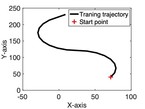
Figure 4: Ground truth trajectory of the training data for $\mathbf{S}_{1}$.

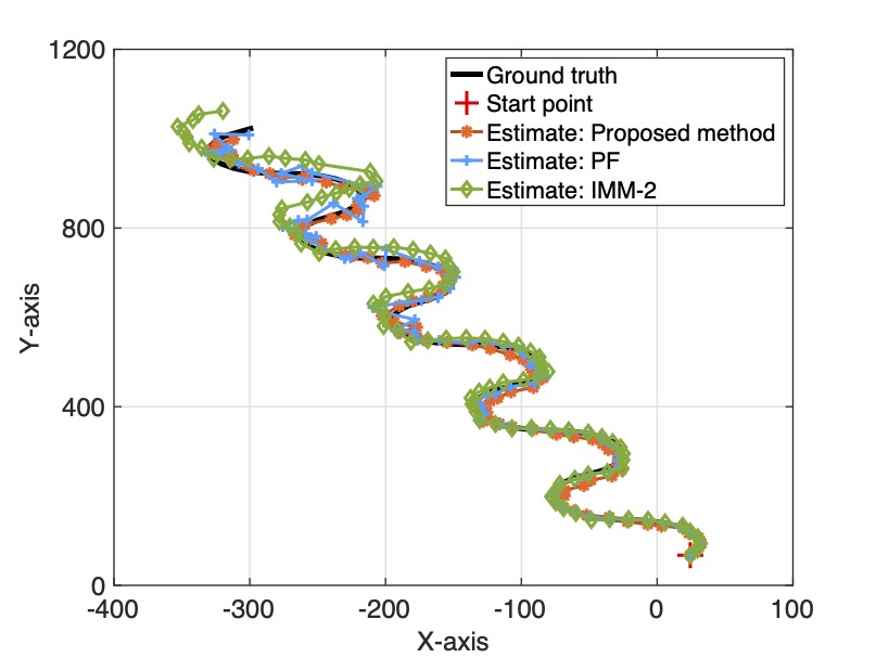
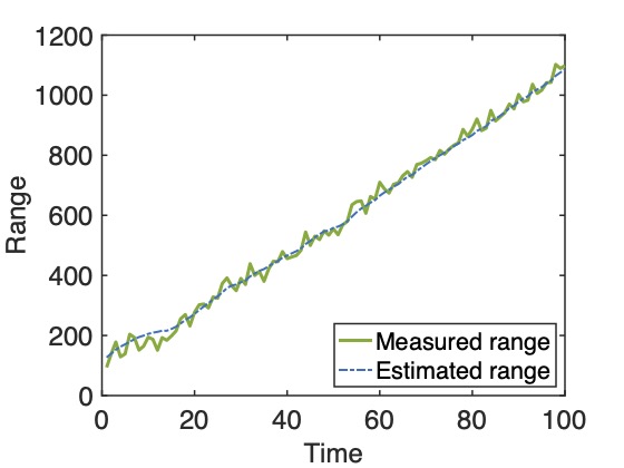
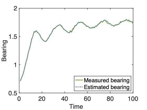
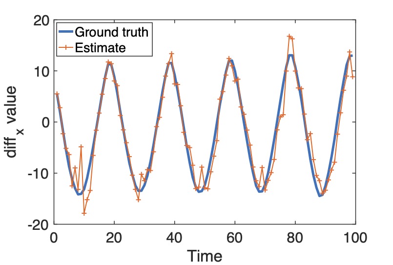
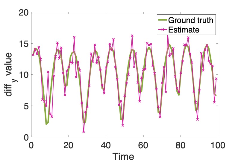
Figure 5: Tracking performance of $\mathcal{GP}_{\textbf{S1}}$ for scenario $\mathbf{S}_{1}$. (a) Tracking trajectories. (b) Measured and estimated range with time. (c) Measured and estimated bearing with time. (d) Estimations of X-axis Cartesian velocities with time. (e) Estimations of Y-axis Cartesian velocities with time.

Table II: Comparisons of RMSE performance for $\mathbf{S_{1}}$

Method	Proposed method	Oracle PF	$\mathrm{IMM-2}$
RMSE – $\mathbf{S_{1}}$	15.5414	$\mathbf{15.1072}$	33.6308

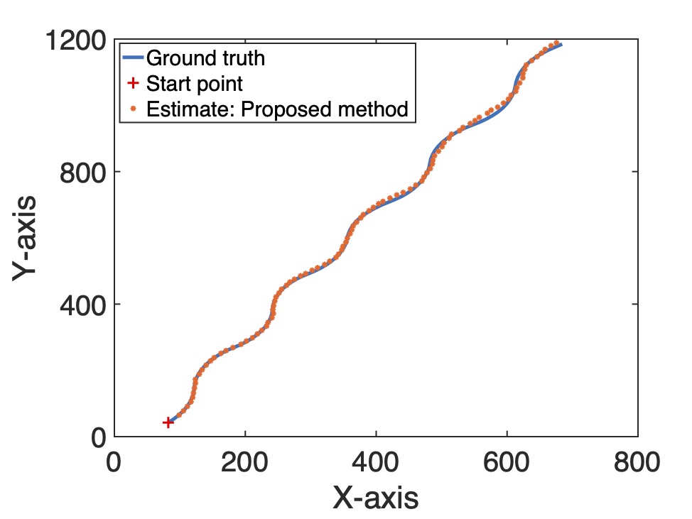
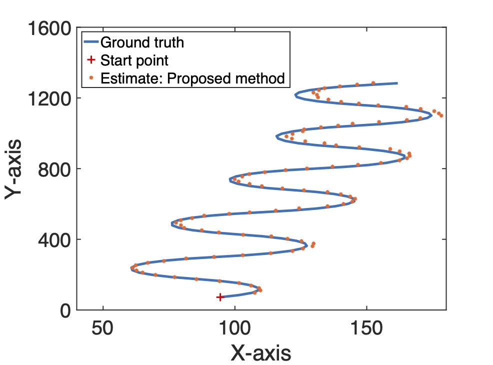
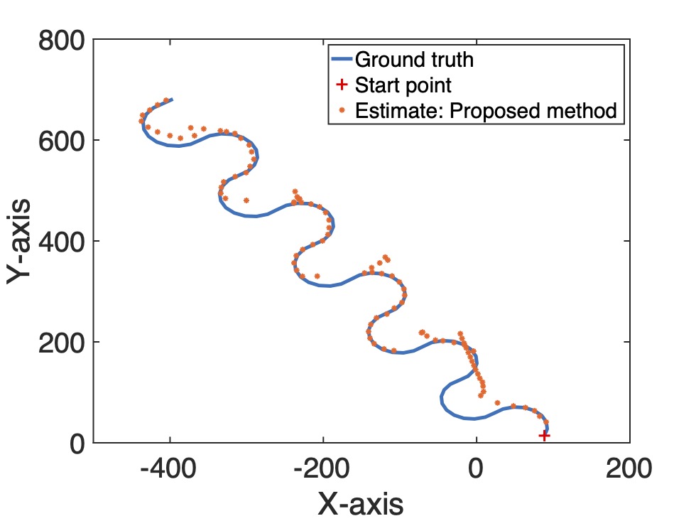
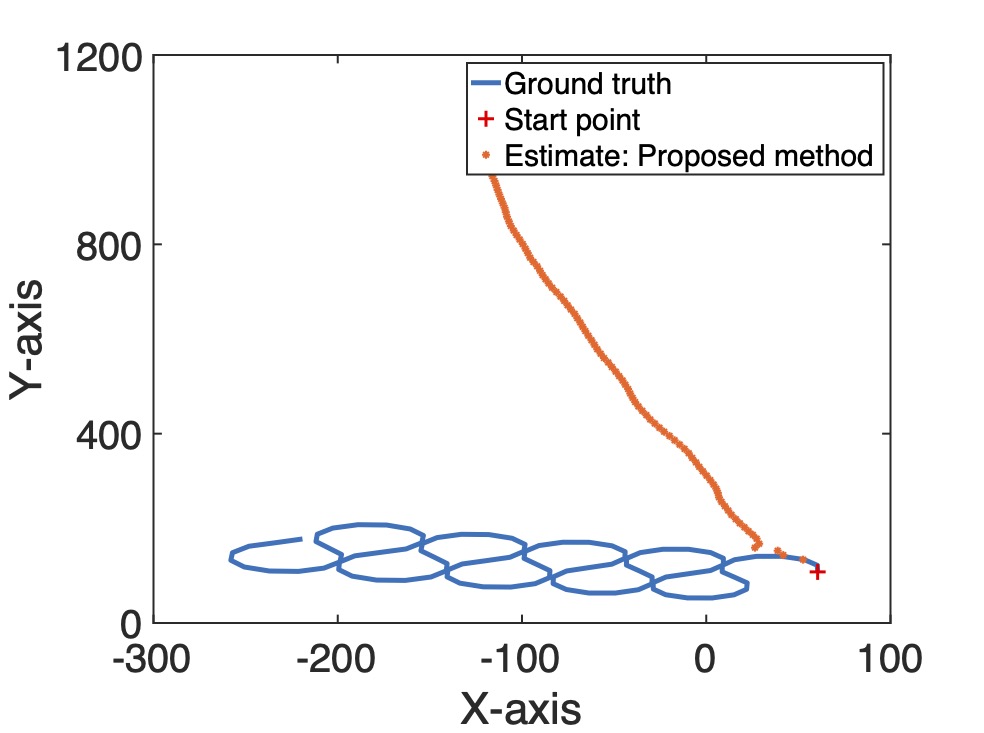
Figure 6: Tracking performance of $\mathcal{GP}_{\textbf{S1}}$ for GCTs with different turn rate sets. $\mathcal{GP}_{\textbf{S1}}$ is trained based on a GCT data set with $\pm 15\circ$. Legend: start point of the moving trajectory. (a) $\pm 5^{\circ}$. (b) $\pm 10^{\circ}$. (c) $\pm 20\circ$. (d) $\pm 30^{\circ}$.

To evaluate the robustness of the trained motion model, the trained GPs based on $\pm 15^{\circ}$ turn rate, i.e. $\mathcal{GP}_{\textbf{S1}}$, are then applied to track the targets which move following the gradual coordinated turns model but with different turn rates, i.e. $\left[\pm 5^{\circ},\pm 10^{\circ},\pm 20^{\circ},\pm 30^{\circ}\right]$. The tracking performance is shown in Fig. 6. We can see that the performance is still favorable when the turn rates are set to be $\pm 5^{\circ}$ and $\pm 10^{\circ}$, i.e. those absolute values are smaller than the turn rate used for training. However, the tracking performance of the proposed method is drastically reduced when the turn rate is $\pm 20^{\circ}$ and loses the tracking when the turn rate is $\pm 30^{\circ}$ which is very far away from the training data turn rate.

V-C2 Motion scenario $\mathbf{S_{2}}$

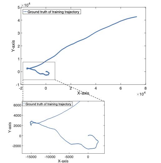
Figure 7: Ground truth trajectory of the training data for $\mathbf{S}_{3}$.

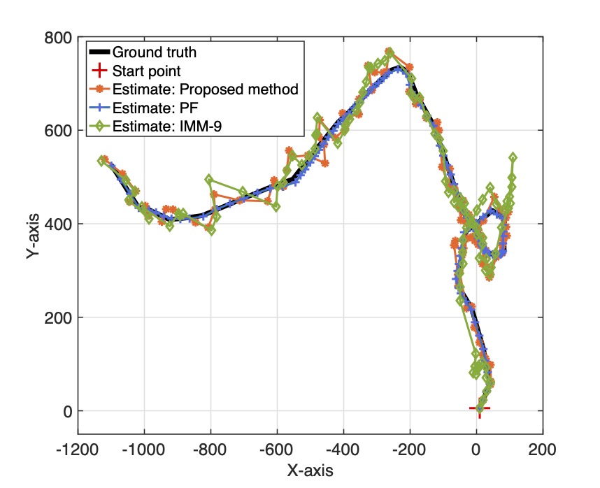
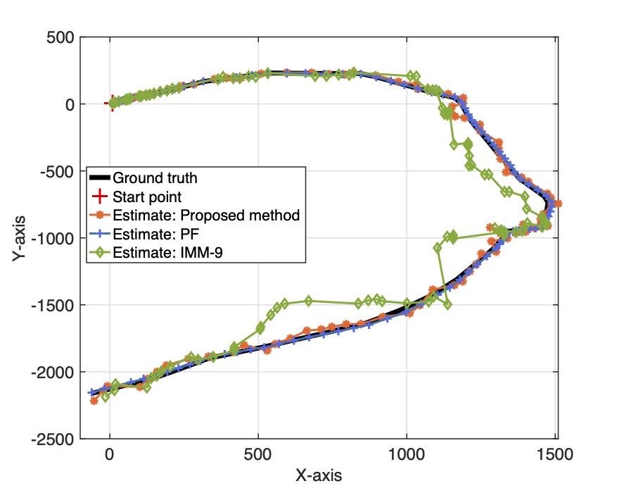
Figure 8: Tracking performance of $\mathcal{GP}_{\textbf{S3}}$. (a) Trajectory–1. (b) Trajectory–2.

The training data length for $\mathbf{S_{2}}$ is $N_{\textbf{S2}}=1000$, and the ground truth trajectory for training is shown in Fig. 7. The learned GP models are represented as $\mathcal{GP}_{\textbf{S2}}$. The test data length and the number of particles are set as $T_{\textbf{S2}}=100$, $M_{\textbf{S2}}=200$, respectively. The ground truth trajectories for training and testing are different, i.e. not from the same dataset, but follow the same motion model. The oracle PF gives the benchmark performance with full prior knowledge of the real-time along-track and cross-track accelerations. The IMM-PF compared is represented as IMM-9. All the potential motion parameters of the test data are set as the candidates of the IMM-PF algorithm, i.e. nine motion models are set as the candidates with ${\alpha}_{t,k}^{t}\in\{0.1,1,10\}$ and ${\alpha}_{t,k}^{n}\in\{0.1,1,10\}$. Fig. 8 and Fig. 8 show the tracking performance comparison of two typical examples. Note that the trajectory in Fig. 7 used for training differs from those used for the actual test experiment, but both are generated following the same motion model. The RMSE performance comparisons obtained for 50 MC realizations are shown in Table III. From the simulation results, we can arrive at the following conclusions. Firstly, the proposed GP-based learning method has good suitability and scalability for different moving trajectory schemes. Secondly, compared with the IMM-PF, the tracking performance of the proposed method is better. Compared with the oracle PF, the performance of the proposed algorithm is similar despite the unknown motion parameters.

Table III: Comparisons of RMSE performance for $\mathbf{S_{2}}$

Method	Proposed method	Oracle PF	IMM-9
RMSE – ${\mathbf{S_{2}}}$	28.9758	14.2775	248.9746

V-D Robustness of Learned GP models

Given that the standard curvilinear-motion kinematics mode is a general motion model that various (noiseless) kinematic models can be derived from, in this experiment, the learned GP model $\mathcal{GP}_{\textbf{S2}}$ and IMM-9 are applied to scenarios with different motion behaviours, e.g. $\mathbf{S}_{1}$ and $\mathbf{S}_{3}$, to evaluate the robustness. $\mathbf{S}_{3}$ is defined as the target moves with random turn rate $\pm 15^{\circ}$s for 1s.

One realization for different scenarios and the RMSE obtained for 50 MC realizations are shown in Fig. 9 and Table IV, respectively. The tracking performance comparisons demonstrate that the learned GP models from more general training data, i.e. the learned GP model $\mathcal{GP}_{\textbf{S2}}$ has good robustness for different moving trajectories following different motion models with the same or lower maneuvering.

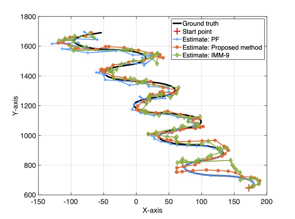
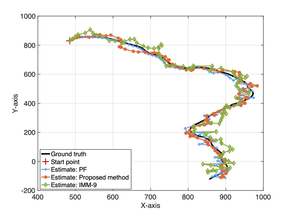
Figure 9: Tracking performance of $\mathcal{GP}_{\textbf{S2}}$. Legend: start point of the moving trajectory. (a) ${\mathbf{S_{1}}}$. (b) ${\mathbf{S_{3}}}$.

Table IV: Comparisons of RMSE performance of $\mathcal{GP}_{\mathbf{S2}}$

Method	Proposed method	Oracle PF	$\mathrm{IMM-9}$
RMSE – $\mathbf{S_{1}}$	15.4871	$\mathbf{10.1769}$	17.8063
RMSE – ${\mathbf{S_{3}}}$	18.0542	$\mathbf{17.4488}$	52.1975

V-E Multi-target Tracking Performance

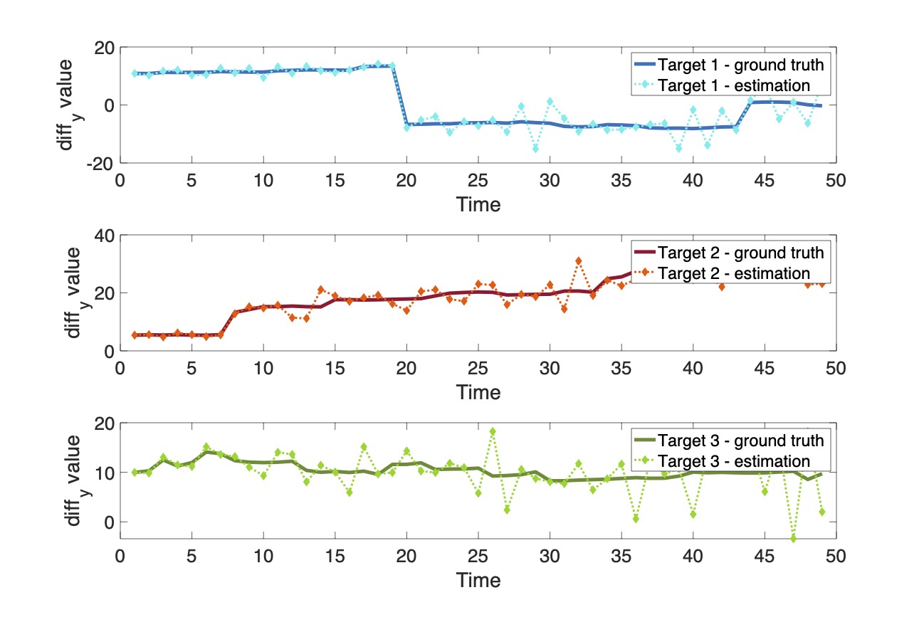
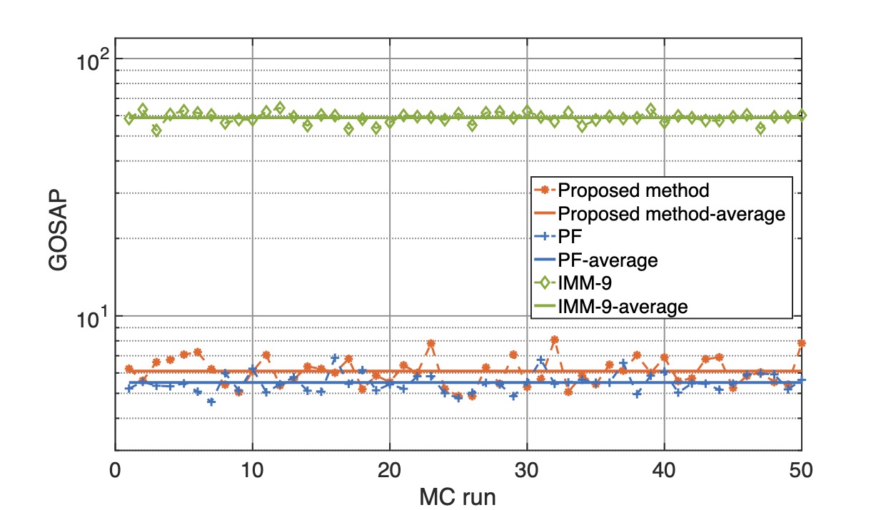
Figure 10: Tracking performance of MTT S2. (a) Estimations of differential X-axis position with time. (b) Estimations of differential Y-axis position with time. (c) Tracking performance of the proposed method. (d) Tracking performance of the PF with real-time accelerations method. (e) Tracking performance of the IMM-9. (f) GOSAP performance of different methods for MTT. The number of targets is 3, and the motion models for all targets follow S2.

The motion behavior of the multi targets is set to follow $\mathbf{S_{2}}$, and the tracking time length is $T=50$. The learned GP model $\mathcal{GP}_{\mathbf{S2}}$ is used for online tracking prediction. The number of particles is $M=500$. The tracking performance for one realization of four different filters is shown in Fig. 10 to Fig. 10. Note that for the compared methods, i.e. the oracle PF and the IMM-9 that includes the accurate motion model, the data association is assumed to be prior knowledge. The generalized optimal sub-patten assignment metric (GOSAP) is used for evaluating the statistical tracking performance as it captures three critical factors: localization errors for correctly detected targets, number of missed detections, and number of false detections due to clutter. The GOSAP is calculated as [30]

$$d_{p}^{(c,\alpha)}(X,\hat{X})=\left(\min_{\pi\in\prod_{\left|\hat{X}\right|}}\sum_{i=1}^{\left|X\right|}d^{c}\left(x_{i},\hat{x}_{\pi(i)}\right)^{p}+\frac{c^{p}}{\alpha}\left(\left|\hat{X}\right|-\left|X\right|\right)\right)^{\frac{1}{p}}.$$ (38)

Here, $X$ and $\hat{X}$ represent the states of true targets and estimations respectively, whose numbers are $\left|X\right|$ and $\left|\hat{X}\right|$. $c>0$, $0<\alpha\leq 2$ and $1\leq p<\infty$. $d(x,\hat{x})$ denote the metric for any $x,\hat{x}\in\mathbb{R}^{N}$ and $d^{(c)}(x,\hat{x})=\min(d(x,\hat{x}),c)$ is its cut-off metric [30]. From the simulation results shown in Fig. 10, we can conclude that compared to the IMM-PF methods with the same number of particles, the proposed particle GP-BP method provides 90% performance improvement in the position estimation, and it can achieve very similar tracking performance to the oracle PF.

VI conclusion

This study proposes a new method for target tracking under unknown motion models. The method proposed is based on GPR, which can learn target movements’ NSIM behaviors. The experiments showed that this method had satisfying accuracy and outstanding robustness for random target trajectories and is still valid when the test data’s surveillance region is outside the training data’s surveillance region. In addition, we demonstrated the immediate potential for using the proposed method as a plug-and-play prediction module in various Bayesian filtering applications.

References

• [1] Z. Liu, Q. Zhang, L. Li, and W. Xie, “Tracking multiple maneuvering targets using a sequential multiple target Bayes filter with jump Markov system models,” Neurocomputing, vol. 216, pp. 183–191, 2016. [Online]. Available: https://www.sciencedirect.com/science/article/pii/S0925231216307731
• [2] B.-T. Vo and B.-N. Vo, “Labeled random finite sets and multi-object conjugate priors,” IEEE Trans. Signal Process., vol. 61, no. 13, pp. 3460–3475, 2013.
• [3] J. Vermaak, S. Godsill, and P. Perez, “Monte Carlo filtering for multi target tracking and data association,” IEEE Trans. Aerosp. Electron. Syst., vol. 41, no. 1, pp. 309–332, 2005.
• [4] R. P. S. Mahler, B.-T. Vo, and B.-N. Vo, “CPHD filtering with unknown clutter rate and detection profile,” IEEE Trans. Signal Process., vol. 59, no. 8, pp. 3497–3513, 2011.
• [5] X. Rong Li and V. Jilkov, “Survey of maneuvering target tracking. Part V. Multiple-model methods,” EEE Trans. Aerosp. Electron. Syst., vol. 41, no. 4, pp. 1255–1321, 2005.
• [6] J. L. Yang, L. Yang, Z. Y. Xiao, and J. J. Liu, “Adaptive parameter particle CBMeMBer tracker for multiple maneuvering target tracking,” EURASIP J. Adv. Signal Process., vol. 2016, pp. 1–11, May 2016.
• [7] L. ZX, W. DH, X. WX, and L. LQ, “Tracking the turn maneuvering target using the multi-target Bayes filter with an adaptive estimation of turn rate,” Sens. (Basel), vol. 17, no. 2, p. 373, 2017.
• [8] J. Son, M. Baek, M. Cho, and B. Han, “Multi-object tracking with quadruplet convolutional neural networks,” in 2017 IEEE Conference on Computer Vision and Pattern Recognition (CVPR), 2017, pp. 3786–3795.
• [9] N. Wahlstrom and E. Ozkan, “Extended target tracking using Gaussian processes,” IEEE Trans. Signal Process., vol. 63, no. 16, pp. 4165–4178, 2015.
• [10] W. Aftab, A. De Freitas, M. Arvaneh, and L. Mihaylova, “A Gaussian process approach for extended object tracking with random shapes and for dealing with intractable likelihoods,” in 2017 22nd International Conference on Digital Signal Processing (DSP), 2017, pp. 1–5.
• [11] S. Jung, I. Schlangen, and A. Charlish, “Sequential Monte Carlo filtering with long short-term memory prediction,” in 2019 22th International Conference on Information Fusion (FUSION), 2019, pp. 1–7.
• [12] A. Sean, B. Timothy, T. ChiHay, and S. Simo, “Batch nonlinear continuous-time trajectory estimation as exactly sparse Gaussian process regression,” Auton. Robots, vol. 39, no. 3, p. 221–238, Oct. 2015.
• [13] W. Aftab and L. Mihaylova, “A learning Gaussian process approach for maneuvering target tracking and smoothing,” IEEE Trans. Aerosp. Electron. Syst., vol. 57, no. 1, pp. 278–292, 2021.
• [14] M. Sun, M. E. Davies, I. Proudler, and J. R. Hopgood, “A Gaussian process based method for multiple model tracking,” in 2020 Sensor Signal Processing for Defence Conference (SSPD), 2020, pp. 1–5.
• [15] M. Arulampalam, S. Maskell, N. Gordon, and T. Clapp, “A tutorial on particle filters for online nonlinear/non-Gaussian Bayesian tracking,” IEEE Trans. Signal Process., vol. 50, no. 2, pp. 174–188, 2002.
• [16] A. Doucet, S. Godsill, and C. Andrieu, “On sequential Monte Carlo sampling methods for Bayesian filtering,” Stat. Comput., vol. 10, 04 2003.
• [17] F. Kschischang, B. Frey, and H.-A. Loeliger, “Factor graphs and the sum-product algorithm,” IEEE Trans. Inf. Theory, vol. 47, no. 2, pp. 498–519, 2001.
• [18] D. Koller and N. Friedman, Probabilistic Graphical Models: Principles and Techniques, ser. Adaptive computation and machine learning.   MIT Press, 2009. [Online]. Available: https://books.google.co.in/books?id=7dzpHCHzNQ4C
• [19] E. Riegler, G. E. Kirkelund, C. N. Manchon, M.-A. Badiu, and B. H. Fleury, “Merging belief propagation and the mean field approximation: A free energy approach,” IEEE Trans. Inf. Theory, vol. 59, no. 1, pp. 588–602, 2013.
• [20] F. Meyer, T. Kropfreiter, J. L. Williams, R. Lau, F. Hlawatsch, P. Braca, and M. Z. Win, “Message passing algorithms for scalable multitarget tracking,” Proc. IEEE, vol. 106, no. 2, pp. 221–259, 2018.
• [21] J. Williams and R. Lau, “Approximate evaluation of marginal association probabilities with belief propagation,” IEEE Trans. Aerosp. Electron. Syst., vol. 50, no. 4, pp. 2942–2959, 2014.
• [22] F. Meyer, P. Braca, P. Willett, and F. Hlawatsch, “A scalable algorithm for tracking an unknown number of targets using multiple sensors,” IIEEE Trans. Signal Process., vol. 65, no. 13, pp. 3478–3493, 2017.
• [23] C.-Y. Chong, “Tracking and data fusion: A handbook of algorithms (bar-shalom, y. et al; 2011) [bookshelf],” IEEE Control Syst., vol. 32, no. 5, pp. 114–116, 2012.
• [24] C. E. Rasmussen and C. K. I. Williams, Gaussian processes for machine learning., ser. Adaptive computation and machine learning.   MIT Press, 2006.
• [25] A. J. Davies, “Effective implementation of Gaussian process regression for machine learning,” Ph.D. dissertation, University of Cambridge, 2015.
• [26] Y. Zhao, C. Fritsche, G. Hendeby, F. Yin, T. Chen, and F. Gunnarsson, “Cramér–Rao bounds for filtering based on Gaussian process state-space models,” IEEE Trans. Signal Process., vol. 67, no. 23, pp. 5936–5951, 2019.
• [27] A. T. Ihler, J. W. F. III, and A. S. Willsky, “Loopy belief propagation: Convergence and effects of message errors,” J. Mach. Learn. Res., vol. 6, pp. 905–936, 2005. [Online]. Available: http://jmlr.org/papers/v6/ihler05a.html
• [28] J. H. Kotecha and P. M. Djuric, “Gaussian particle filtering,” IEEE Trans. Signal Process, vol. 51, no. 10, pp. 2592–2601, 2003.
• [29] X. Rong Li and V. Jilkov, “Survey of maneuvering target tracking. Part I. Dynamic models,” IEEE Trans. Aerosp. Electron. Syst., vol. 39, no. 4, pp. 1333–1364, 2003.
• [30] A. S. Rahmathullah, A. F. Garcia-Fernandez, and L. Svensson, “Generalized optimal sub-pattern assignment metric,” in 2017 20th International Conference on Information Fusion (Fusion), 2017, pp. 1–8.