On Quantum Entropy and Excess Entropy Production in a System-Environment Pure State

Abstract

We explore a recently introduced quantum thermodynamic entropy $S^{Q}_{univ}$ of a pure state of a composite system-environment computational “universe” with a simple system $\mathcal{S}$ coupled to a constant temperature bath $\mathcal{E}$. The principal focus is “excess entropy production” in which the quantum entropy change is greater than expected from the classical entropy-free energy relationship. We analyze this in terms of quantum spreading of time dependent states, and its interplay with the idea of a microcanonical shell. The entropy takes a basis-dependent Shannon information definition. We argue for the zero-order $\mathcal{SE}$ energy basis as the unique choice that gives classical thermodynamic relations in the limit of weak coupling and high density of states, including an exact division into system and environment components. Entropy production takes place due to two kinds of processes. The first is classical “ergodization” that fills the full density of states within the microcanonical shell. The second is excess entropy production related to quantum spreading or “quantum ergodization” of the wavepacket that effectively increases the width of the energy shell. Lorentzian superpositions with finite microcanonical shell width lead to classical results as the limiting case, with no excess entropy. We then consider a single $\mathcal{SE}$ zero-order initial state, as the examplar of extreme excess entropy production. Systematic formal results are obtained for a unified treatment of excess entropy production for time-dependent Lorentzian superpositions, and verified computationally. It is speculated that the idea of free energy might be extended to a notion of “available energy” corresponding to the excess entropy production. A unified perspective on quantum thermodynamic entropy is thereby attained from the classical limit to extreme quantum conditions.

I introduction

This paper concerns “excess entropy production” in simulations of a system-environment pure state, using a recently devised quantum thermodynamic entropy for a pure state. These ideas arise out of new developments in quantum thermodynamics. Recent years have seen a renewal of interest in the foundations of quantum statistical mechanics, both for theoretical reasons and practical interests of new technologies. A prominent line of research has investigated thermodynamic behavior in pure state systems micro ; deltasuniv ; twobath ; variabletame ; polyadbath ; Belgians2 ; Olshanni ; Gemmer:2009 ; Rudolph ; tasaki1998 . Arguments based on the “eigenstate thermalization hypothesis” Deutsch ; RigolReview ; Greiner2016 ; Deutsch1991 ; DeutschSupplemental ; Porras ; Leitner2015 ; Leitner2018 ; Rigol and “typicality” Goldstein2006 ; Goldstein2010 ; vNcommentary ; Reimann2008 ; Popescu2009 ; Popescu2006 ; Reimann2016 ; Goldstein2015 stake a persuasive claim that thermalization is a property of entanglement in pure states of complex systems. Nonetheless, we have called attention to an apparent gap in the quantum thermodynamics of pure states. The classical second law states that in spontaneous processes, the “entropy of the universe” is always increasing

$$\Delta S_{univ}>0$$ (1)

with the following relation between free energy and entropy change:

$$-\frac{1}{T}\ \Delta F_{sys}=\Delta S_{univ}.$$ (2)

However, these relations seem to be missing in quantum thermodynamics of a pure state, because the standard von Neumann quantum entropy is zero for such a state. In Refs. deltasuniv ; micro we defined a quantum entropy $S^{Q}_{univ}$ for a pure system-environment (SE) state, compared this with $\Delta F_{sys}$, and found that we could recover the microcanonical limit Eq. 2 for equilibration and thermalization. These results seem to justify calling $S^{Q}_{univ}$ a thermodynamic entropy for a pure state. To a certain extent, our approach goes back to interest of von Neumann himself in new ideas of quantum entropy vNtrans ; vNcommentary . Others have introduced ideas somewhat related to ours of the entropy of a pure state both for analyzing pure state thermodynamics HanEntropy ; PolkovnikovicEntropy and characterizing the information content of pure states KakEntropy ; informationentropystotland .

The focus of the present paper is excess entropy production: thermodynamic entropy $\Delta S^{x}$ beyond what is implied in the classical relation Eq. (2). This is a quantum phenomenon that was noted in Refs. deltasuniv ; micro , in the course of exploring the classical microcanonical limit in which Eq. 2 holds. Excess entropy production can lead to distinctly non-classical processes. We have shown twobath that these can include surprising phenomena such as heat flow from cold to hot and asymmetric temperature equilibration in a tripartite total system. In the present work, the goal is a deeper systematic account of this excess entropy production and its physical meaning. A unified understanding is sought of the quantitative behavior of $\Delta S^{x}$ between extreme limits of zero (i.e. classical) and maximal, massive excess entropy. Concepts of density of states, quantum spreading of states, and Boltzmann entropy come into play. It should be possible to control excess entropy by “tuning” the initial state. We anticipate that this understanding will be useful for devising and analyzing highly unusual, nonclassical situations in quantum thermodynamics of complex systems.

An outline of the paper is likely useful. Section II summarizes the model system $\mathcal{S}$ and environment $\mathcal{E}$. Section III deals with the definition of the quantum thermodynamic entropy for a pure $\mathcal{SE}$ state and Section IV concerns the formal division of the entropy into system and environment parts. Section V emphasizes heuristically that excess entropy production takes place almost entirely in the environment, with the excess occurring due to quantum spreading of the wavepacket. This insight is then examined computationally and formally in the succeeding sections. Lorentzian wave packets turn out to be ideally suited for this. In Section VI time-evolving Lorentzian states are constructed, and their dynamics simulated computationally. Section VII examines analytic and computational “master relations” for the quantum entropy $S^{Q}_{univ}$ and the excess entropy $\Delta S^{x}$ in the near-classical and extreme-quantum limits. Section VIII gives a summing-up and ends with some speculation about excess “free” or “available” energy associated with excess entropy production.

II Model system and environment

The model system $\mathcal{S}$ and environment $\mathcal{E}$ are taken from Ref. micro . The system has evenly spaced levels. The environment is designed to mimic a standard heat bath with a constant temperature $T$. Small environments with time- and size-dependent temperatures are also of interest in other contexts variabletame , but our main concern here is to understand quantum thermodynamics in the standard limit where the bath is large. To model a large bath, we use a discrete approximation to a true continuum of environment states, with density of states

$$\rho_{\mathcal{E}}(E_{\mathcal{E}})=Ae^{E_{\mathcal{E}}/T}$$ (3)

with the Boltzmann constant $k_{B}=1$. We consider the temperature as the fixed value $T=6.22$ energy units throughout the evolution of all $\mathcal{SE}$ states we consider. We use a system with three evenly spaced energy levels $\{|s\rangle\}=\{|0\rangle,|1\rangle,|2\rangle\}$ with energies $E_{s}=s$. The system and environment interact through a random matrix coupling with diagonal elements set to zero and off-diagonal elements taken as random Gaussian variates scaled by a coupling constant $k$ that determines the strength of the interaction. Typically we take $A=1415.3$ and $k=0.9\times 10^{-4}$, except in Sec. VII.3. Details of the model are given in Ref. micro .

A schematic of the time evolution behavior is shown in Fig. 1. The system begins in a single zero-order energy level $|s\rangle$, the environment begins in a superposition of zero-order levels $|\epsilon\rangle$ (we consider variations to environment state later, down to a single energy level $|\epsilon\rangle$), and the total density of $\mathcal{SE}$ states is $\rho_{0}=\rho_{\mathcal{E}}(E_{\mathcal{E}})$. The system and environment then interact, exchange heat and evolve to equilibrium, resulting in the final state on the right. In the final state there are a variety of entangled system-environment components, shown by matching colors in the diagram, each with approximately the same total energy $E=E_{\mathcal{E}}+E_{\mathcal{S}}$, with a total density of states $\rho_{f}(E)=\sum_{s}\rho_{\mathcal{E}}(E-E_{s})$. The system alone is described by a thermal Boltzmann distribution $p_{s}\sim e^{-E_{s}/T}$, related to the exponentially increasing density of environment states at higher energy. This is the schematic view of the system, environment, and thermalization process whose properties we examine in this paper.

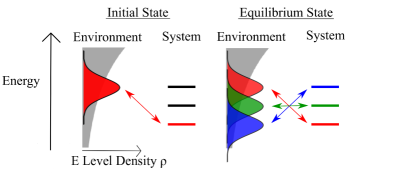
Figure 1: Schematic of time evolution behavior, beginning with a superposition state in the environment and a single zero-order level in the system, then evolving to a thermalized set of entangled system-environment pairs.

III basis set and pure state quantum thermodynamic entropy

First we consider the formal definition and rationale for the pure state quantum entropy $S^{Q}_{univ}$. The definition of $S^{Q}_{univ}$ will depend on a choice of basis set. Our treatment of the basis set expands upon the more cursory justification offered in Ref. deltasuniv . Our choice is the zero-order $\mathcal{SE}$ energy basis. In this and following sections we argue that this, and likely only this choice, will allow recovery of classical microcanonical results, including the Boltzmann distribution, the canonical ensemble, the identity in Eq. 2 in the limit of weak coupling, and the standard microcanonical relation $\Delta S_{env}=Q/T$ between entropy change of the environment and heat flow.

To define the entropy we first choose a “reference basis” $\{|\alpha\rangle\}$. In this basis a pure state is expressed as

$$|\Psi_{\mathcal{SE}}(t)\rangle=\sum_{\alpha}c_{\alpha}(t)|\alpha\rangle.$$ (4)

Then taking

$$p_{\alpha}(t)=|c_{\alpha}(t)|^{2}$$ (5)

we define the quantum entropy

$$S^{Q}_{univ}=S^{\{\alpha\}}_{univ}=-\sum_{\alpha}p_{\alpha}\ln p_{\alpha}$$ (6)

with respect to the reference basis $\{|\alpha\rangle\}$. This expression for the entropy has an evident relation to the Shannon information entropy. In the quantum context it has been discussed as the “conditional information entropy” by Stotland et al. informationentropystotland . One of our goals has been to develop and exploit a thermodynamic meaning for this entropy.

This entropy depends on the choice of reference basis. We choose the zero-order energy basis

$$\{|\alpha\rangle\}=\{|s\rangle|\epsilon\rangle\}$$ (7)

of the $\mathcal{SE}$ complex. Let the total state be expanded in terms of zero-order system-environment energy bases $\{|s\rangle\}$ and $\{|\epsilon\rangle\}$:

$$|\Psi\rangle=\sum_{s,\epsilon}c_{s,\epsilon}|s\rangle|\epsilon\rangle$$ (8)

with $\{|s\rangle\}$ and $\{|\epsilon\rangle\}$ the ZO basis sets of system and environment. Eqs. 4-8 comprise the essence of our quantum entropy. What is the rationale for this? We will be simulating a quantum total system $\mathcal{SE}$ in which energy flows between a system $\mathcal{S}$ and an environment $\mathcal{E}$ – a process of heat flow. In statistical mechanics we typically have in mind measurement of an $\mathcal{S}$ energy level, e.g.  the energy of a Brownian particle in a gravitational field. This mirrors the choice of the zero-order system basis. Then, if we are concerned with thermalizing energy flow, the most natural further observation would be of the zero-order energy of $\mathcal{E}$ to give a total zero order energy of $\mathcal{SE}$. This naturally leads to the basis of ZO energy states $\{|\alpha\rangle\}=\{|s\rangle|\epsilon\rangle\}$. We might not be so interested in measuring the energy of $\mathcal{E}$ – that would be the usual case in the analogy to the Brownian particle. Nonetheless, there are further grounds to favor the $\mathcal{SE}$ zero-order basis. We are naturally interested in constructs that relate to the microcanonical ensemble for a fixed total energy. Since we are interested in observing the $\mathcal{S}$ zero-order energy, the natural way of getting something like a total energy would seem to be as the sum E_SE = E_S + E_E, i.e. the sum of zero order energies, congruent with standard reasoning in the microcanonical ensemble. Having singled out the $\mathcal{S}$ states and the energy sum $E$, the obvious basis is then the zero-order $\mathcal{SE}$ basis. This justification seems compelling, but we will introduce further arguments based on the idea of a division of the entropy $S^{Q}$ into system and environment components, to which we turn in the next two sections.

IV $S^{Q}_{unv}$ as a sum of system and environment terms

In this section we show how the quantum entropy of Eqs. 4-8 can be divided into a sum of system and environment components. The system component comes from the reduced density matrix; the environment component is an averaged sum of contributions, weighted by system probabilities. We begin with the general expression for the Shannon entropy of a bipartite system

$$S=-\sum_{i,\lambda}p_{i,\lambda}\ln p_{i,\lambda}.$$ (9)

We will split this into separate parts for $i$ and $\lambda$, following Neilsen and Chuang nielsenchuangSenv . To begin, define the total probability for $i$ as

$$p_{i}=\sum_{\lambda}p_{i,\lambda}.$$ (10)

Define the conditional probability for $\lambda$ when the first index is $i$ as

$$p_{\lambda|i}=\frac{p_{i,\lambda}}{p_{i}}.$$ (11)

Using the newly defined probabilities and the normalization $\sum_{\lambda}p_{\lambda|i}=1$ the entropy becomes nielsenchuangSenv

$$S=-\sum_{i,\lambda}p_{i}p_{\lambda|i}\ln p_{i}p_{\lambda|i}=-\sum_{i}p_{i}\ln p_{i}+\sum_{i}p_{i}\left(-\sum_{\lambda}p_{\lambda|i}\ln p_{\lambda|i}\right)$$

$$=S_{i}+\langle S_{\lambda}\rangle_{\{i\}}.$$ (12)

Eq. 12 gives the general decomposition of the Shannon entropy of a bipartite system into separate parts for the two systems. The entropy $S_{i}$ is a standard Shannon entropy for the first system. The second system has a conditional entropy $\langle S_{\lambda}\rangle_{\{i\}}$ that is averaged with respect to the probabilities $p_{i}$ for the first system.

Now consider the quantum entropy Eq. 6 with $\{|\alpha\rangle\}=\{|s\rangle|\epsilon\rangle\}$ as the reference basis of system-environment zero-order energy states and $p_{\alpha}=p_{s,\epsilon}=|c_{s,\epsilon}|^{2}$. The entropy can be separated into system and environment parts, in parallel with Eq. 12:

$$S^{Q}_{univ}=S^{Q}_{\mathcal{S}}+S_{\mathcal{E}}^{Q}.$$ (13)

The system entropy

$$S^{Q}_{\mathcal{S}}=-\sum_{s}p_{s}\ln p_{s}$$ (14)

uses system probabilities that can be calculated from the reduced density matrix with diagonal elements $p_{s}=\sum_{\epsilon}p_{s,\epsilon}=\langle s|\hat{\rho}_{\mathcal{S}}|s\rangle$. $S_{\mathcal{S}}^{Q}$ agrees with the standard quantum von Neumann entropy of the system when $\hat{\rho}_{\mathcal{S}}$ is dephased in the system zero-order energy basis $\{|s\rangle\}$, as in the Boltzmann thermal state and our initial state. The environment entropy is then

$$S_{\mathcal{E}}^{Q}=\sum_{s}p_{s}\left(-\sum_{\epsilon}p_{\epsilon|s}\ln p_{\epsilon|s}\right).$$ (15)

with $p_{\epsilon|s}=p_{s,\epsilon}/p_{s}$. Eqs. 13-15 give our procedure for calculating the total entropy $S^{Q}_{univ}$ in terms of system $S^{Q}_{\mathcal{S}}$ and environment $S_{\mathcal{E}}^{Q}$ parts.

V entropy production in the environment: density of states and quantum spreading

We have shown how to decompose the total entropy change $\Delta S_{univ}^{Q}$ into separate parts $\Delta S_{\mathcal{S}}^{Q}$ and $\Delta S_{\mathcal{E}}^{Q}$ for the system and environment. Now we give a heuristic argument for how to relate these to their classical microcanonical counterparts $\Delta S_{sys}^{\mathrm{micro}}$ and $\Delta S_{\mathcal{E}}^{\mathrm{micro}}$. We will find that excess entropy production is a component of the environment entropy change beyond the classical $Q/T.$ We will find later in Section VII that this correlates with analytical results for Lorentzian superposition states in our numerical simulations.

First consider the classical entropy change during system-environment thermalization. The system and environment begin in isolation, corresponding to a microcanonical ensemble of $W_{0}=\rho_{0}\delta E$ states with entropy $S_{univ,0}^{\mathrm{micro}}=\ln W_{0}$, where $\rho_{0}$ is the initial density of states and $\delta E$ is the width of the microcanonical energy shell. The system and environment then exchange heat, evolving to fill a larger set of $W_{f}=\rho_{f}\delta E$ states. The microcanonical entropy change is

$$\ln\frac{\rho_{f}}{\rho_{0}}=\Delta S_{univ}^{\mathrm{micro}}=\Delta S_{\mathcal{S}}^{\mathrm{micro}}+\Delta S_{\mathcal{E}}^{\mathrm{micro}}$$ (16)

where the last equality uses Eq. 12. The environment entropy change in Eq. 16 is given by the standard relation between the heat $Q$ and temperature $T$,

$$\Delta S_{\mathcal{E}}^{\mathrm{micro}}=Q/T,$$ (17)

as shown in detail in Supplemental Information Sec. A (Eq. A22). We now show how these quantities can be related to their quantum counterparts.

As anticipated in our previous work micro , and developed analytically for time-dependent states in Section VII and Supplemental Information Sec. C (Eq. (C14)), the quantum entropy change can be analyzed in terms of a microcanonical-like relation

$$S^{Q}_{univ}\sim\ln W_{eff}$$ (18)

with an effective number of states $W_{eff}=\rho\delta E$, and a variable effective energy width $\delta E$. The width generally increases because of quantum state spreading during the dynamical equilibration process. This results in a greater width for the final equilibrium state than the initial state $\delta E_{f}>\delta E_{0}$. Then the total entropy change is

$$\Delta S_{univ}^{Q}\approx\ln\frac{\rho_{f}}{\rho_{0}}+\ln\frac{\delta E_{f}}{\delta E_{0}}$$ (19)

This is a key relation. The “double logarithm of ratios” form is very suggestive. It is obtained heuristically here and analytically later in Eqs. 35,36 for time-evolving Lorentzian states. There are two sources of entropy change. The first term $\ln\rho_{f}/\rho_{0}$ is the classical system-environment entropy change from Eq. 16. It might be loosely referred to as due to “classical ergodization.” The second term is the excess entropy production. It is due to quantum spreading or “quantum ergodization” of the energy shell:

$$\Delta S^{x}=\ln\frac{\delta E_{f}}{\delta E_{0}}.$$ (20)

We now use the system-environment decomposition of the entropy Eq. 13 to show that $\Delta S^{x}$ is contained entirely within the environment. Note that the quantum and classical entropy changes of the system are the same $\Delta S^{Q}_{sys}=\Delta S_{sys}^{\mathrm{micro}}$ since in both cases the system thermalizes to a Boltzmann distribution. Then expressing $\Delta S_{univ}^{Q}$ on the left of Eq. 19 in terms of system and environment parts we have that the quantum entropy change of the environment is

$$\Delta S_{\mathcal{E}}^{Q}\approx\Delta S_{\mathcal{E}}^{\mathrm{micro}}+\ln\frac{\delta E_{f}}{\delta E_{0}}=\frac{Q}{T}+\Delta S^{x}$$ (21)

with the approximation indicated because this is a heuristic argument, in keeping with Eq. 19. The quantum entropy change of the environment is thus generally greater than the classical $Q/T$, with excess entropy production related to the increase in the width of the quantum energy shell.

With this analysis at hand, we return to the question of the justification for the $\mathcal{SE}$ zero order reference basis in defining $S^{Q}_{univ}$ in Eqs. 4-7 of Section III. Our decomposition of $S^{Q}_{univ}$ into system and environment parts gives standard results in the classical limit for a fixed microcanonical shell: $\Delta S_{\mathcal{S}}^{Q}=\Delta S_{\mathcal{S}}^{\mathrm{micro}}$ and $\Delta S_{\mathcal{E}}^{Q}=Q/T$. Other choices of basis would give different values for the entropy changes. This strongly supports the choice of the $\{|s\rangle|\epsilon\rangle\}$ reference basis as the unique basis that gives standard results in the classical microcanonical limit.

VI Time evolving Lorentzian states

Now we relate the preceding heuristic considerations to two concrete situations of Lorentzian wavepackets that are illuminating for being computationally transparent and analytically tractable. We obtain analytical results for the entropy production from these states and confirm predictions in calculations, expanding on previous results micro from a more heuristic approach.

Ref. micro observed in computations with different types of initial superposition states that there was excess entropy production. In the weak coupling/infinite density of states limit this excess entropy went to zero, and classical microcanonical results were obtained: the free energy – entropy relation Eq. 2. Ref. micro was about time evolution of a wave packet constructed from a superposition of many $\mathcal{SE}$ zero order states. The initial wave packet had a single $\mathcal{S}$ state and many $\mathcal{E}$ states in the product. The idea was to mimic an initial state reasonably close to classical, within a microcanonical energy shell, with the width of the shell corresponding to the range of environment zero order energies. The classical limit was obtained as the coupling $k$ and density of states $\rho$ were varied.

However, it is not yet so clear under what general conditions classical behavior will be recovered, and what governs the magnitude of excess entropy production. What role is played by the width of the microcanonical shell, of both initial and final states, in determining the magnitude of excess entropy? Here we probe this by comparing the time evolution of two very different types of initial state, which are meant to serve as extreme cases. One is a Lorentzian superposition of many $\mathcal{SE}$ initial states, corresponding to a microcanonical shell of significant width, with the expectation of quasi-classical behavior. The second is a single zero order $\mathcal{SE}$ state. Here the width of the microcanonical shell is essentially zero. The surmise is that nonclassical effects of excess entropy production will be extreme with this latter state.

Figure 2: Average probabilities $|\langle s|\langle\epsilon|\Psi\rangle|^{2}$ for nearby $|s\rangle|\epsilon\rangle$ basis states for (a) an initial Lorentzian state from Eq. 22 with half-width at half-max $\gamma_{0}=0.5$ and (b) the corresponding time-evolved state of Eq. 27. The asymmetric error bars show the first and third quartiles of the distribution of probabilities that go into the averages shown by the data points. (c) Entropy production $\Delta S_{univ}^{Q}$ and free energy change $-\Delta F_{sys}/T$ during the time evolution.

Figure 3: Average probabilities $|\langle s|\langle\epsilon|\Psi\rangle|^{2}$ for nearby $|s\rangle|\epsilon\rangle$ basis states for (a) an initial $|s\rangle|\epsilon\rangle$ state from Eq. 26 and (b) the corresponding time-evolved state of Eq. 27. The asymmetric error bars show the first and third quartiles of the distribution of probabilities that go into the averages shown by the data points. (c) Entropy production $\Delta S_{univ}^{Q}$ and free energy change $-\Delta F_{sys}/T$ during the time evolution.

VI.1 Initial states

We investigate these questions with two kinds of simulations. One takes a random superposition of $\mathcal{SE}$ zero-order states under an overall Lorentzian window. The second takes a single $\mathcal{SE}$ zero-order state – an extreme case of a Lorentzian, with zero width. The results, shown in Figs. 2,3, will be critically discussed in the following sections. Reasons for considering Lorentzians are as follows. The energy eigenstates are Lorentzian superpositions of zero order states, as pointed out by Deutsch in his introduction Deutsch1991 of the eigenstate thermalization hypothesis (ETH). Following analysis of Supplemental Information Sec. B, a single $|s\rangle|\epsilon\rangle$ zero-order state then consists of a Lorentzian superposition of eigenstates, which then evolves into a Lorentzian of zero-order states. An initial Lorentzian time-dependent superposition evolves into a (wider) Lorentzian superposition. Thus, with Lorentzian initial states, down to the limit of zero-width Lorentzian $|s\rangle|\epsilon\rangle$ states, we evolve to Lorentzian final states. This gives a unified class of states for systematic analysis. There are analytical results that can be brought to bear on the statistics of these Lorentzians, and also the entropy production. Furthermore, the Lorentzian width has a nice correspondence to the idea of a microcanonical shell width. Hence, Lorentzians are ideally suited for the systematic quantitative investigation of entropy production that we want to undertake.

We will consider initial states with the system in a single level $|s\rangle$ and the environment described by fluctuations $\tilde{g}_{s,\epsilon}$ about a Lorentzian distribution $L^{0}_{s,\epsilon}$

$$|\Psi^{0}_{L}\rangle\sim\sum_{\epsilon}\tilde{g}_{s,\epsilon}\sqrt{L_{s,\epsilon}^{0}}|s\rangle|\epsilon\rangle$$ (22)

The Lorentzian distribution at time $t=0$ is

$$L_{s,\epsilon}^{0}(E_{s}+E_{\epsilon})=\frac{1}{\pi}\frac{\gamma_{0}/\rho_{0}}{(E_{s}+E_{\epsilon}-E_{0})^{2}+\gamma_{0}^{2}}$$ (23)

where $\rho_{0}$ is the density of environment states that pair with the initial system level $|s\rangle$ and $E_{0}$ and $\gamma_{0}$ are parameters that respectively describe the central energy of the Lorentzian and the half-width at half-max. The $\tilde{g}_{s,\epsilon}$ are complex random gaussian variates that give random deviations to the $|s\rangle|\epsilon\rangle$ basis state probabilities about the Lorentzian average. These are taken as as

$$\tilde{g}_{s,\epsilon}=\frac{g_{s,\epsilon}+ig^{\prime}_{s,\epsilon}}{\sqrt{2}}$$ (24)

where $g_{s,\epsilon}$ and $g^{\prime}_{s,\epsilon}$ are random numbers from Gaussian distributions, e.g.

$$p(g_{s,\epsilon})=\frac{1}{\sqrt{2\pi}}e^{-g_{s,\epsilon}^{2}/2}$$ (25)

Panel (a) of Fig. 2 shows an example of an initial state with random variations about a Lorentzian as in Eq. 22 with an initial width $\gamma_{0}=0.5$. The data points in the figure are averaged squared coefficients $|c_{s,\epsilon}|^{2}=|\langle s|\epsilon|\Psi\rangle|^{2}$, averaged over all $|s\rangle|\epsilon\rangle$ states in an energy interval, with asymmetric error bars indicating the first and third quartiles of the coefficient distributions in the intervals. The average squared coefficients follow the Lorentzian from Eq. 23. The error bars are in good agreement with the quartiles expected from the Gaussian random deviations $\tilde{g}_{s,\epsilon}$, as discussed in detail in the Supplemental Information.

We will also be concerned with the time-evolution of initial single $|s\rangle|\epsilon\rangle$ basis states

$$|\Psi^{0}_{s,\epsilon}\rangle=|s\rangle|\epsilon\rangle$$ (26)

These can be viewed as the limit $\gamma_{0}\to 0$ of the random Lorentzian initial states in Eq. 22, where the Lorentzian distribution approaches a $\delta$ function. Fig. 3(a) shows an $|s\rangle|\epsilon\rangle$ initial state as in Eq. 26, with just a single nonzero coefficient $c_{s,\epsilon}=1$. This is an example of a very non-classical starting state, where the “width” of the initial microcanonical energy shell is zero and the probability density is a delta function.

VI.2 Time evolution and quantum spreading

Now consider the time evolution of the random Lorentzian states of Eq. 22 and of the single $|s\rangle|\epsilon\rangle$ states of Eq. 26. We find in the Supplemental Information that both of these evolve to equilibrium states that can be described statistically by random fluctuations about a Lorentzian average, in accord with previous analyses of Deutsch Deutsch1991 ; DeutschSupplemental and Nation and Porras Porras in a similar model. The final states are given as

$$|\Psi_{L}^{f}(t)\rangle,|\Psi_{s,\epsilon}^{f}(t)\rangle\sim\sum_{s,\epsilon}\tilde{g}_{s,\epsilon}\sqrt{L_{f}}|s\rangle|\epsilon\rangle$$ (27)

with a final state Lorentzian

$$L_{f}(E_{s}+E_{\epsilon})=\frac{1}{\pi}\frac{\gamma_{f}/\rho_{f}}{(E_{s}+E_{\epsilon}-E_{0})^{2}+\gamma_{f}^{2}}$$ (28)

where $\rho_{f}$ is the total density of $|s\rangle|\epsilon\rangle$ states and $\gamma_{f}$ is the half-width at half-max of the final Lorentzian, to be discussed further below.

The half-width at half-max $\gamma_{f}$ is found in the Supplemental Information to be increased by the “spreading factor” $2\pi k^{2}\rho$ relative to the initial state width $\gamma_{0}$:

$$\gamma_{f}=\gamma_{0}+2\pi k^{2}\rho_{f},$$ (29)

where $k$ is the coupling strength and $\rho_{f}(E)=\sum_{s}\rho_{\mathcal{E}}(E-E_{s})$ is the total density of states at equilibrium, following Sec. II. Eqs. 27-29 apply to both the equilibrated, time-evolved Lorentzian initial states of Eq. 22 and the time-evolved $|s\rangle|\epsilon\rangle$ states of Eq. 26, where for the latter it is understood that the value $\gamma_{0}=0$ is used in the final width in Eq. 29, so that $\gamma_{f}=2\pi k^{2}\rho_{f}$.

Panel (b) of Figs. 2 and 3 show the time-evolved states. Both states spread in time. Both evolve to random fluctuations about the Lorentzians $L_{f}$ from Eq. 28 with the appropriate widths $\gamma_{f}$ from Eq. 29. The variations in the coefficients are very well characterized by the Gaussian random variations $\tilde{g}_{s,\epsilon}$ in Eq. 27. See the Supplemental Information Section B for details.

VI.3 Entropy Production for the Time-Evolving $|s\rangle|\epsilon\rangle$ and Lorentzian States

Now we consider the entropy production for these examples of time-evolving states. Panel (c) of Fig. 2 shows the entropy production $\Delta S_{univ}^{Q}$ as the initial Lorentzian superposition in (a) evolves to the wider final Lorentzian distribution in (b). $\Delta S_{univ}^{Q}$ is compared with the classical entropy change $-\Delta F_{sys}/T=\Delta S_{univ}^{\mathrm{micro}}$, which we compute using the standard definition $F_{sys}=\langle E_{\mathcal{S}}\rangle-TS^{vN}_{\mathcal{S}}$, with $S^{vN}_{\mathcal{S}}$ the von Neumann entropy. There is some excess entropy production, as expected from Ref. micro , but overall it is fairly close to microcanonical. Figure 3(c) shows the entropy production for the initial single $|s\rangle|\epsilon\rangle$ state that evolves to a final random Lorentzian. Now there is a very large amount of excess entropy production. It seems that the finite microcanonical shell width of the initial state in Fig. 2 plays an essential role in getting the approach to classical behavior, because it limits the relative spreading of the wave packet in time, as suggested by Eq. 20. To understand these connections systematically, we will take advantage of analytic expressions for superposition states with a Lorentzian profile, using results from Supplemental Information Sec. B. We will see that considerable insight is gained following this path. We will see that we can “tune” the excess entropy production between the classical limit of zero for a suitable Lorentzian, and the very large excess of a single $|s\rangle|\epsilon\rangle$ state, as suggested in Figs. 2 and 3 and seen systematically in Figs. 4 - 6, to which we turn next.

VII master relationships for $S^{Q}_{univ}$ and $\Delta S^{x}$ for time-evolving Lorentzian states

Now we want to attain a systematic understanding of the entropies in these simulations and how they change during equilibration, in comparison with the analytical results for the initial and final state statistics in Section VI. The basic results, seen in Figs. 4 - 6, show evident regularities, which we briefly remark upon before detailed consideration. The initial states are either random Lorentzians or a single $|s\rangle|\epsilon\rangle$ basis state, as in Eqs. 22 and 26. We will find that the entropies for these two types of initial states can be united in the analytic “master entropy” Eq. 33, which accounts for the pattern of Fig. 4. Both types of initial states evolve to final states that are also random Lorentzians, as in Eq. 27. This will lead to an analytical expression for the expected excess entropy production in Eq. 39 and Fig. 5. Finally, we consider the question of entropy production in approach to the classical limit, building on our earlier investigation of related but distinct questions in Ref. micro . Fig. 6 will show that superposition states approach classical entropy production $\Delta S^{x}=0$ while the $|s\rangle|\epsilon\rangle$ initial states are at a much different, opposite extreme. We will be able to account for the regularities in Figs. 4 - 6 in accord with our earlier heuristic arguments about $S^{Q}$ and $\Delta S^{x}$ in Section V, based on ideas about the microcanonical shell and quantum spreading of the environment state during equilibration. We begin with analysis of entropy production and excess entropy production with a fixed model for the environment and $\mathcal{SE}$ coupling in Figs. 4-5, then analyze how variations in the size and coupling strength affect the entropy production for Lorentzian and $|s\rangle|\epsilon\rangle$ initial states in Fig. 6.

VII.1 Entropy of the States

We will find an analytic relationship for the entropy of the Lorentzian states, related to Boltzmann’s entropy formula $S=k\ln W$ and the idea of a microcanonical shell width. This is attained following the derivation in Supplemental Information Sec. C (Eq. (C.14)). The results, displayed in Fig. 4, show an interesting relationship between the analytic predictions and computed entropies. We now outline the derivation and meaning of these results. The derivation approximates the fundamental sum for the entropy Eq. 6 as an integral over the random Lorentzian coefficients, such as appear in Eqs. 22 and 27. The integral approximation is justified when the Lorentzian is wide relative to the $\mathcal{SE}$ energy level spacing. The result is that the entropy for the Lorentzian is

$$S_{L}=\ln(4\pi\gamma\rho)-g_{0}$$ (30)

where $\rho$ is the density of states and $\gamma$ is the half-width at half-max of the Lorentzian. These have the values $\rho_{0}$ and $\gamma_{0}$ for the initial Lorentzian states, as appear in Eq. 23, and $\rho_{f}$ and $\gamma_{f}$ for the final states, as described in the discussion around Eq. 29.

The first term on the right of Eq. 30 gives the entropy of a perfect Lorentzian (without the random variations $\tilde{g}_{s,\epsilon}$). This has the microcanonical-like form suggested previously in Eq. 18,

$$\ln(4\pi\gamma\rho)=\ln(\rho\delta E)=\ln W_{eff}$$ (31)

with $W_{eff}=\rho\delta E$ an effective number of states in an energy shell of width $\delta E=4\pi\gamma$. We compute the second term in (30) using Mathemtica and find

$$g_{0}=\langle|\tilde{g}_{s,\epsilon}|^{2}\ln|\tilde{g}_{s,\epsilon}|^{2}\rangle=1-\gamma_{EM}.$$ (32)

This gives the deviation from the Lorentzian entropy due to the random fluctuations in the basis state probabilities $\tilde{g}_{s,\epsilon}$, with $\gamma_{EM}=0.577\ 215...$ the Euler-Mascheroni constant WolframEulerMascheroni (See Supplemental Information Sec. C for details). Using this value of $\gamma_{EM}$, $g_{0}=0.422\ 785...$. We have thus obtained the desired relationship between $S^{Q}_{univ}$, Boltzmann’s entropy formula, and the number of states with a given shell width and density of states.

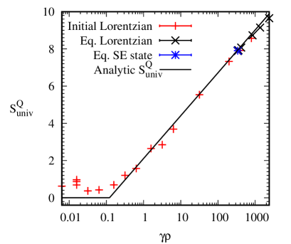
Figure 4: Entropies from initial Lorentzian states (Eq. 22) with varying widths $\gamma_{0}$, time-evolved version of these states at equilibrium, and a time-evolved $|s\rangle|\epsilon\rangle$ state at equilibrium all approximately follow the analytic $S^{Q}_{univ}$ from Eq. 33.

How well this works is seen numerically in Fig. 4 which shows the computational entropies for three kinds of initial states: a time-evolved $|s\rangle|\epsilon\rangle$ state; initial states with random variations about a Lorentzian, from Eq. 22, with various initial widths $5\times 10^{-6}\leq\gamma_{0}\leq 0.25$; and the time-evolved Lorentzian states with final widths $\gamma=\gamma_{f}$ from Eq. 29. The simulation results are well described by the approximate $S_{L}$ of Eq. 30 along the diagonal line of the figure, when $\gamma\rho$ is not too small. For small $\gamma\rho$ on the left of the figure, the initial states approach the limit of the single $|s\rangle|\epsilon\rangle$ basis state, which of course has entropy $\ln(1)=0$. In this limit, the integral approximation that goes into the derivation of $S_{L}$ breaks down. It gives $S_{L}<0$ when $\gamma<e^{g_{0}}/4\pi\rho$, whereas $S^{Q}_{univ}\geq 0$ by definition. A better approximate formula is obtained by setting the entropy to zero when $S_{L}$ becomes negative, essentially approximating the entropy of the very narrow states by the value 0 for a single $|s\rangle|\epsilon\rangle$ state. This gives the complete generic “master” formula for the entropy of the time evolving random Lorentzian states, plotted as a solid line:

$$S^{Q}_{univ}\approx\left\{\begin{array}[]{lll}\ln(4\pi\gamma\rho)-g_{0}&:&\gamma\geq e^{g_{0}}/4\pi\rho\\ 0&:&\mathrm{otherwise}\\ \end{array}\right.$$ (33)

This is the same as the previous relation $S_{L}$, except that it stops changing when it reaches the minimum value zero, giving the abrupt bend in the figure. The simulation results are in good agreement with this predicted behavior, with fluctuations around $S^{Q}_{univ}=0$ at small $\gamma\rho$, and following the curve for $S_{L}$ at larger $\gamma\rho$. The results show the master relation for $S^{Q}_{univ}$ holds for initial Lorentzian states and time-evolved versions of those states. For an initial $|s\rangle|\epsilon\rangle$ state the entropy is zero in accord with the master relation, and the figure shows that a time evolved $|s\rangle|\epsilon\rangle$ state is also in agreement with the general trend. In sum, the approximate master entropy relation Eq. 33 is giving a good account of the simulation results for all the initial and final states we consider. We next use this relation to understand the excess component $\Delta S^{x}$ of the entropy production, as depicted in Fig. 5. Finally, we analyze this entropy production in the question of approach to classical microcanonical behavior in the standard limit of a large bath and weak coupling, finding diverging results for “normal” superpositions and “extreme” $|s\rangle|\epsilon\rangle$ initial states in Fig. 6.

VII.2 Entropy Production

We next consider entropy production, including excess entropy production, during the approach to equilibrium. The aim is to see how entropy production relates to the intuitive ideas of the width of the microcanonical shell and the of spreading of the quantum wave packet. First, we consider initial states with random variations about a Lorentzian from Eq. 23 that are well described by the approximate entropy $S_{L}$ of Eq. 30, when $\gamma_{0}\geq e^{g_{0}}/4\pi\rho_{0}$ in Eq. 33. The entropy change in time evolution from initial to final state is

$$\Delta S_{L}=\ln(4\pi\gamma_{f}\rho_{f})-g_{0}-\left(\ln(4\pi\gamma_{0}\rho_{0})-g_{0}\right)$$ (34)

based on the initial and final values of $S_{L}$ from Eq. 30. Cancelling terms gives

$$\Delta S_{L}=\ln\frac{\rho_{f}}{\rho_{0}}+\ln\frac{\gamma_{f}}{\gamma_{0}}.$$ (35)

This is the second appearance of the “double logarithm of ratios” form, noted earlier in connection with Eq. 19. The first term $\ln\rho_{f}/\rho_{0}$ gives the classical entropy change from heat flow, following the microcanonical definition Eq. 16, in a process of “classical ergodization.” The second term gives the quantum excess entropy production

$$\Delta S_{L}^{x}=\ln\frac{\gamma_{f}}{\gamma_{0}}=\ln\frac{\delta E_{f}}{\delta E_{0}}$$ (36)

due to quantum spreading or “quantum ergodization” of the environment state wave packet. This analytic relation is similar to the somewhat more complicated empirical curve for fitting $\Delta S^{x}$ in Ref. micro with a less structured type of $\mathcal{SE}$ state, which did not maintain a consistent Lorentzian profile as we have here. For our Lorentzians we obtain the simple formula of Eq. 36, in terms of only the initial and final Lorentzian widths $\gamma_{0}$ and $\gamma_{f}$. This corresponds transparently to the increase in the effective width of the energy shell, as anticipated in Eq. 20.

The diagonal line on the left of Fig. 5 shows the analytic $\Delta S_{L}^{x}$ of Eq. 36 compared with $\Delta S^{x}=\Delta S_{univ}^{Q}+\Delta F_{sys}/T$ from the simulations. Moving from left to right in the figure, we are decreasing $\gamma_{0}$ to increase the ratio $\gamma_{f}/\gamma_{0}$. The approximate relation is giving a good account of the results on the left of the figure, where $\gamma_{f}/\gamma_{0}$ is not too large.

Now consider the right side of Fig. 5. The $\Delta S^{x}$ are reaching close to the maximum value, i.e.  for a single $|s\rangle|\epsilon\rangle$ state, corresponding to the limit of small $\gamma_{0}$ with large $\gamma_{f}/\gamma_{0}$. For small $\gamma_{0}$, we want to take the initial state as the limiting single $|s\rangle|\epsilon\rangle$ state, like what we did for $S^{Q}_{univ}$ in Eq. 33. For a single $|s\rangle|\epsilon\rangle$ initial state the initial entropy is zero. The final state has the Lorentzian entropy $S_{L}$. Then $\Delta S_{univ}^{Q}=S_{L}$. The maximum excess entropy production is then calculated by subtracting the microcanonical $\ln\rho_{f}/\rho_{0}$ ,

$$\Delta S^{x,max}=\ln(4\pi\gamma_{f}\rho_{f})-g_{0}-\ln\frac{\rho_{f}}{\rho_{0}}.$$ (37)

To evaluate this equation, we use $\gamma_{f}$ from Eq. 29, with $\gamma_{0}=0$ for the $|s\rangle|\epsilon\rangle$ initial state. This gives

$$\Delta S^{x,max}=\ln(8\pi^{2}k^{2}\rho_{f}\rho_{0})-g_{0}.$$ (38)

We now have the “master” equation for the excess entropy production

$$\Delta S^{x}\approx\left\{\begin{array}[]{lll}\ln(\gamma_{f}/\gamma_{0})&:&\gamma_{0}\geq e^{g_{0}}/4\pi\rho_{0}\\ \ln(8\pi^{2}k^{2}\rho_{f}\rho_{0})-g_{0}&:&\mathrm{otherwise}\\ \end{array}\right.$$ (39)

This master relation for $\Delta S^{x}$ is shown by the black solid line in Fig. 5. It follows $\Delta S^{x}_{L}$ from Eq. 36 up until this reaches the maximum value for a single $|s\rangle|\epsilon\rangle$ initial state, where the master relation bends and becomes flat in the right of the figure. This is in good agreement with our simulation results, which follow $\Delta S^{x}_{L}$ in the left of the figure then fluctuate around the maximum value in the right of the figure. In sum, we are getting a good systematic account of the excess entropy production.

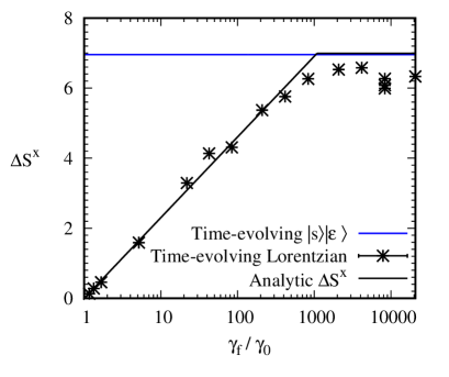
Figure 5: Excess entropy production for initial random Lorentzians (black stars) and for an initial $|s\rangle|\epsilon\rangle$ state (blue bar) follow the master equation Eq. 39.

VII.3 Excess Entropy Production and the Microcanonical Limit

We have seen that the source of excess entropy production is the relative increase in the width of the environment state from quantum spreading during equilibration. Larger $\gamma_{f}/\gamma_{0}$ gives greater deviations from a fixed microcanonical energy shell, with larger $\Delta S^{x}$. What has not been brought out so far is the role of the size of the environment and the $\mathcal{SE}$ coupling strength. We have been dealing with a finite model environment with finite coupling, in contrast to the textbook situation with an infinite environment $\rho_{f}\to\infty$ and negligible coupling $k\to 0$. Ref. micro showed with superposition states that microcanonical results $\Delta S^{x}=0$ were obtained in the limit $k\to 0,\rho_{f}\to\infty$ with $k\rho_{f}=const$, as needed to maintain thermalization within the simulations. Ref.  6 had a quite different context than the analysis of Figs. 4 and 5, which have a fixed density of states and coupling, and the extreme range of initial width from wide superpositions to single $|s\rangle|\epsilon\rangle$ initial states. Now the question is how the choice fo the initial shell width affects the approach the classical limit $\Delta S^{x}=0$ as we increase the bath size and decrease the coupling.

Fig. 6 shows $\Delta S^{x}$ in a series of calculations heading toward the supposed “microcanonical limit” $k\to 0,\rho_{f}\to\infty$, with $k\rho_{f}=const$; this is accomplished by taking the baseline values for $k$ and the density of states prefactor $A$, noted below Eq. (3), and varying these with $A\sim 1/k$ and $Ak=const.$. First consider the Lorentzian states in the figure, with small values of $\Delta S^{x}$. These clearly approach classical behavior $\Delta S^{x}=0$ from the right as quantum spreading becomes negligible, with $\gamma_{f}\to\gamma_{0}$ in Eq. 29 and therefore $\Delta S^{x}\to 0$ in Eq. 36. Now consider the $|s\rangle|\epsilon\rangle$ states in the figure. They have very nearly constant computational $\Delta S^{x}\approx\Delta S^{x,max}$, as predicted by Eqs. 38 and 39. The maximum $\Delta S^{x}$ for an $|s\rangle|\epsilon\rangle$ initial state depends only on the products $k\rho_{f}$ and $k\rho_{0}$, which are both constant as we approach the limit, so there is no hint at all of approach to classical behavior. Instead, quantum spreading is always significant and classical behavior is never observed for the $|s\rangle|\epsilon\rangle$ states. For intermediate cases between the two extremes in Fig. 6, it should be possible to “tune” the excess entropy, as emphasized previously.

This completes our investigation of entropy content of states, entropy production including excess, and the question of what kinds of states approach the classical limit, within our range of “normal” and “extreme” states.

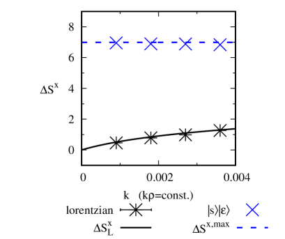
Figure 6: Excess entropy production for Lorentzian initial states with widths $\gamma_{0}=0.0625$ and $|s\rangle|\epsilon\rangle$ initial states, with model environments having variable $k\rho$ constant, heading towards the microcanonical limit $k\to 0,\rho\to\infty,k\rho=const.$ in the bottom left. The Lorentzians approach the classical result $\Delta S^{x}=0$, the $|s\rangle|\epsilon\rangle$ states do not.

VIII summary and concluding remarks

We have systematically explored the phenomenon of excess entropy production in time-dependent equilibration processes, in terms of the quantum thermodynamic entropy of Refs. micro ; deltasuniv for a system-environment pure state. Our focus is the role of quantum spreading of the $\mathcal{SE}$ state, its relation to the width of the microcanonical energy shell, and violation of the classical entropy-free energy relation in the form of excess entropy production. We span the range from near-classical behavior to the extreme of excess entropy with a single zero-order initial state.

Using the Shannon information entropy definition, we defined the quantum entropy $S^{Q}_{univ}$ in terms of the zero-order energy basis. This choice of basis is made on the grounds that thermodynamically one would be interested in observation of the system zero-order state, so that straightforward definition of the energy in the microcanonical shell necessitates the sum of zero-order system and environment energies. We showed that there is a mathematical division of $S^{Q}_{univ}$ into system and environment terms. With this, we found that our choice of basis for the definition of $S^{Q}_{univ}$ uniquely gives standard thermodynamic results in the classical limit of weak coupling and large density of states, with the standard classical relations $\Delta S_{univ}=-\Delta F_{sys}/T$ and $\Delta S_{env}=Q/T$. The entropy is readily understood with Boltzmann’s equation $S=k\ln W$, with $W$ being given by shell width $\times$ density of states $\delta E\times\rho=4\pi\gamma\rho$ according to Eq.  30.

$\Delta S^{Q}_{univ}$ can be understood for Lorentzian states, as being due to two components. One is “classical ergodization” as the system thermalizes and heat flows into the environment, with consequent increase in the occupied density of states, giving the contribution $\ln\rho_{f}/\rho_{0}$. The second is excess entropy production $\Delta S^{x}$ due to quantum spreading or “quantum ergodization” of the microcanonical shell, represented by $\ln\gamma_{f}/\gamma_{0}$ in Eq.  39. The excess happens in the environment – not as heat flow $Q/T$ within the original, “classical” microcanonical shell, but rather as quantum spreading of the shell. The final width of the Lorentzian $\gamma_{f}$ increases by an additive factor independent of the initial width $\gamma_{0}$, so the initial width $\gamma_{0}$ is a critical factor in the ratio $\ln\gamma_{f}/\gamma_{0}$ that determines $\Delta S^{x}$. Hence, initial states like a microcanonical wave packet with small relative spreading $\gamma_{f}/\gamma_{0}\approx 1$ approach the classical limit. On the other hand, initial states that approach the extreme limit of a single $\mathcal{SE}$ zero order state have maximal, massive entropy production, very different from classical.

In sum, we have the following picture. The quantum entropy $S^{Q}_{univ}$ describes time-dependent thermodynamic evolution. In the limit of small coupling, large bath, and non-zero initial energy-shell width, the classical limit is recovered. Away from this limit, there is excess entropy production $\Delta S^{x}>0$. This excess is due to time-dependent quantum spreading. In general, it can be quite large, much larger than the classical entropy production, with a single $\mathcal{SE}$ zero-order state being the extreme case. As we have seen, it is easy to “tune” wave packets between the classical limit of zero excess entropy production, and the limit of extreme entropy production by a single zero-order state. One can speculate that $\Delta S^{x}$ represents excess expenditure of a kind of available or free energy. In this connection, we have shown that excess entropy can be associated with distinctly nonclassical effects in quantum systems, such as heat flow from cold to hot and asymmetric temperature equilibration twobath . It could be very interesting to try to relate such effects to the quantitative treatment of excess entropy developed here.

Acknowledgment

This work benefitted from access to the Talapas supercomputer at the University of Oregon.

Supplemental Information

Here we present Supplemental Information to the main paper: “On Quantum Entropy and Excess Entropy Production in a System-Environment Pure State.”

A: Analysis of the system-environment decomposition of the classical microcanonical entropy

We show how a system-environment decomposition of the classical microcanonical Boltzmann entropy $S=k_{B}\ln W$ gives the standard result for the environment $\Delta S^{\mathrm{micro}}_{\mathcal{E}}=Q/T$ in Eq. 17 of the main text.

The classical microcanonical ensemble is based on the idea of $W=\rho\delta E$ states in the microcanonical energy shell of width $\delta E$ with density of states $\rho$. The entropy is given by Boltzmann’s relation

$$S_{univ}^{\mathrm{micro}}=-\sum_{s,\epsilon}p_{s,\epsilon}^{\mathrm{micro}}\ln p_{s,\epsilon}^{\mathrm{micro}}=\ln W,$$ (40)

where

$$p_{s,\epsilon}^{\mathrm{micro}}=\frac{1}{W}.$$ (41)

The entropy can be decomposed into system and environment parts following Eq. 12 of the main text,

$$S_{univ}^{\mathrm{micro}}=S_{\mathcal{S}}^{\mathrm{micro}}+S_{\mathcal{E}}^{\mathrm{micro}}.$$ (42)

First consider the system component, analogous to $S_{i}$ in Eq. 12 of the main text,

$$S_{\mathcal{S}}^{\mathrm{micro}}=-\sum p_{s}^{\mathrm{micro}}\ln p_{s}^{\mathrm{micro}},$$ (43)

with system probabilities computed from Eq. 41 as

$$p_{s}^{\mathrm{micro}}=\sum_{\epsilon=1}^{W_{s}}p_{s,\epsilon}^{\mathrm{micro}}=\frac{W_{s}}{W},$$ (44)

where $W_{s}$ is the number of bath states $\epsilon$ that pair with $s$ in the microcanonical ensemble. Using Eq. 44 to rewrite $\ln p_{s}^{\mathrm{micro}}$ in Eq. 43 gives

$$S_{\mathcal{S}}^{\mathrm{micro}}=-\sum_{s}p_{s}^{\mathrm{micro}}(\ln W_{s}-\ln W)=\ln W-\sum_{s}p_{s}^{\mathrm{micro}}\ln W_{s}$$ (45)

Now consider the environment term

$$S_{\mathcal{E}}^{\mathrm{micro}}=\sum_{s}p_{s}^{\mathrm{micro}}\left(-\sum_{\epsilon}p_{\epsilon|s}^{\mathrm{micro}}\ln p_{\epsilon|s}^{\mathrm{micro}}\right)$$ (46)

analogous to $\langle S_{\lambda}\rangle_{\{i\}}$ in Eq. 12 of the main text. The conditional environment probabilities are calculated from Eq. 11 of the main text along with Eqs. 41 and 44,

$$p_{\epsilon|s}^{\mathrm{micro}}=\frac{p_{s,\epsilon}^{\mathrm{micro}}}{p_{s}^{\mathrm{micro}}}=\frac{1}{W_{s}}$$ (47)

Using Eq. 47 we can simplify the rightmost sum in Eq. 46

$$-\sum_{\epsilon}p_{\epsilon|s}^{\mathrm{micro}}\ln p_{\epsilon|s}^{\mathrm{micro}}=\ln W_{s},$$ (48)

then putting this into Eq. 46 gives

$$\langle S_{\mathcal{E}}^{\mathrm{micro}}\rangle_{\{sys\}}=\sum_{s}p_{s}^{\mathrm{micro}}\ln W_{s}.$$ (49)

The system and environment entropies Eqs. 45 and 49 clearly sum to the total microcanonical entropy $S_{univ}^{\mathrm{micro}}=\ln W$ in Eq. 40, as needed.

We now consider a thermalization process where we begin with a constrained microcanonical ensemble of $W_{0}$ states for the initial state. For example, this could correspond to a situation where the system begins in thermal isolation from the environment. The constraint is then removed, allowing heat to flow between the system and environment, resulting in a final state microcanonical ensemble with $W_{f}>W_{0}$. The total entropy change is

$$\Delta S_{univ}^{\mathrm{micro}}=\ln\frac{W_{f}}{W_{0}}=\ln\frac{\rho_{f}}{\rho_{0}}$$ (50)

The last equality comes from the microcanonical relation $W=\rho\delta E$ with $\rho$ the density of states in the microcanonical energy shell of width $\delta E$. The system entropy change from Eq. 45 is

$$\Delta S_{\mathcal{S}}^{\mathrm{micro}}=\ln\frac{W_{f}}{W_{0}}-\sum_{s_{f}}p_{s_{f}}^{\mathrm{micro}}\ln W_{s_{f}}+\sum_{s_{0}}p_{s_{0}}^{\mathrm{micro}}\ln W_{s_{0}}$$ (51)

The system entropy change can be greatly simplified through a series of manipulations we will perform on the final two sums of Eq. 51. This will lead to the final simple result for the system entropy in Eq. 59, and will also be useful in deriving the environment entropy change in Eq. 61. First, the sums can be combined by inserting the identities $\sum_{s_{0}}p_{s_{0}}^{\mathrm{micro}}=\sum_{s_{f}}p_{s_{f}}^{\mathrm{micro}}=1$,

$$-\sum_{s_{f}}p_{s_{f}}^{\mathrm{micro}}\ln W_{s_{f}}+\sum_{s_{0}}p_{s_{0}}^{\mathrm{micro}}\ln W_{s_{0}}=-\sum_{s_{0},s_{f}}p_{s_{0}}^{\mathrm{micro}}p_{s_{f}}^{\mathrm{micro}}\ln\frac{W_{s_{f}}}{W_{s_{0}}}.$$ (52)

This is simplified by noting that for a heat bath environment $W\sim e^{E_{\mathcal{E}}/T}$, where $E_{\mathcal{E}}=E_{total}-E_{s}$ is the energy of the environment. Then the ratio $W_{s_{f}}/W_{s_{0}}$ in the right of Eq. 52 can be expressed as

$$W_{s_{f}}/{W_{s_{0}}}=e^{-(E_{s_{f}}-E_{s_{0}})/T}$$ (53)

where $E_{s_{f}}-E_{s_{0}}=\Delta E_{\mathcal{S}}$ is the energy difference between the final and initial system states $s_{f}$ and $s_{0}$. Putting this into Eq. 52 gives

$$-\sum_{s_{0},s_{f}}p_{s_{0}}^{\mathrm{micro}}p_{s_{f}}^{\mathrm{micro}}\ln\frac{W_{s_{f}}}{W_{s_{0}}}=\sum_{s_{0},s_{f}}p_{s_{0}}^{\mathrm{micro}}p_{s_{f}}^{\mathrm{micro}}\frac{E_{s_{f}}-E_{s_{0}}}{T}$$ (54)

Now we separate again into two terms

$$\sum_{s_{0},s_{f}}p_{s_{0}}^{\mathrm{micro}}p_{s_{f}}^{\mathrm{micro}}\frac{E_{s_{f}}-E_{s_{0}}}{T}$$

$$=\frac{1}{T}\left(\sum_{s_{0}}p_{s_{0}}^{\mathrm{micro}}\sum_{s_{f}}p_{s_{f}}^{\mathrm{micro}}E_{s_{f}}-\sum_{s_{f}}p_{s_{f}}^{\mathrm{micro}}\sum_{s_{0}}p_{s_{0}}^{\mathrm{micro}}E_{s_{0}}\right)$$ (55)

Using the identities $\sum_{s}p_{s_{0}}^{\mathrm{micro}}=\sum_{s}p_{s_{f}}^{\mathrm{micro}}=1$ this becomes

$$\frac{1}{T}\left(\sum_{s_{f}}p_{s_{f}}^{\mathrm{micro}}E_{s_{f}}-\sum_{s_{0}}p_{s_{0}}^{\mathrm{micro}}E_{s_{0}}\right)=\frac{\langle E_{\mathcal{S},f}\rangle-\langle E_{\mathcal{S},0}\rangle}{T}=\frac{\Delta\langle E_{\mathcal{S}}\rangle}{T}$$ (56)

Finally, we note that the system energy change is due solely to heat flow from the environment $\Delta\langle E_{\mathcal{S}}\rangle=-Q=-\Delta\langle E_{\mathcal{E}}\rangle$, so we can express the result in Eq. 56 equivalently as

$$\frac{\Delta\langle E_{\mathcal{S}}\rangle}{T}=\frac{-Q}{T}.$$ (57)

In total, Eqs. 52-57 show that

$$-\sum_{s_{f}}p_{s_{f}}^{\mathrm{micro}}\ln W_{s_{f}}+\sum_{s_{i}}p_{s_{0}}^{\mathrm{micro}}\ln W_{s_{0}}=\frac{-Q}{T}$$ (58)

Putting this into Eq. 51 the system entropy change takes the standard and simple final form

$$\Delta S_{\mathcal{S}}^{\mathrm{micro}}=\ln\frac{W_{f}}{W_{0}}-\frac{Q}{T}.$$ (59)

Now consider the entropy change of the environment. From the basic relation of Eq. 49 this is

$$\Delta S_{\mathcal{E}}^{\mathrm{micro}}=\sum_{s_{f}}p_{s_{f}}^{\mathrm{micro}}\ln W_{s_{f}}-\sum_{s_{0}}p_{s_{0}}^{\mathrm{micro}}\ln W_{s_{0}}.$$ (60)

Using Eq. 58 this is simply

$$\Delta S_{\mathcal{E}}^{\mathrm{micro}}=\frac{Q}{T},$$ (61)

which is the standard thermodynamic result. Note this is an exact equality for a standard heat bath with the level density behavior of Eq. 53. Thus we have demonstrated $\Delta S_{\mathcal{E}}^{\mathrm{micro}}=Q/T$, as stated in Eq. 17 of the main text.

B: Lorentzian state distributions

In this appendix we show how we obtain the time-evolving Lorentzian states discussed in Section VI of the main text. The time-evolution of an initial state $|\Psi(0)\rangle$ follows the Schrödinger equation, expressed in terms of the eigenstates $|\xi\rangle$ as

$$|\Psi(t)\rangle=e^{-i\hat{H}t}|\Psi(0)\rangle=\sum_{\xi}c_{\xi}e^{-iE_{\xi}t}|\xi\rangle.$$ (62)

Our approach will be to first analyze the structure of the eigenstates $|\xi\rangle$, then use the eigenstate structure to analyze the time-dependent behavior of the $|s\rangle|\epsilon\rangle$ and Lorentzian initial states.

Some of our important results for the average equilibrium behavior of time-dependent states, Eqs. 64 and 77 below, were obtained in nearly the same form by Deutsch in his well-known paper of 1991 [14, 15] where he developed the ideas behind the eigenstate thermalization hypothesis approach to quantum thermodynamics [11]. Our model varies somewhat from Deutsch’s, so that our eigenstates require an additional parameter in Eq. 64 that was not included in Deutsch’s work. The widths of the eigenstates in from our calculations also vary from Deutsch’s result by a factor of two, in agreement with a recent re-evaluation of Deutsch’s work by Nation and Porras in Ref. [16].

In addition to analyzing the average equilibrium behavior of time-dependent states, we also analyze the fluctuations of a time-evolving state about its average and to develop the idea of a time-evolving initial Lorentzian state. This provides the critical relations in Eq. 27 of the main, appearing again in this appendix as Eqs. 69 and 83.

B.1 Eigenstates

We build up to an analysis of time-dependent states beginning with the structure of the eigenstates $|\xi\rangle$, for the system of a few energy levels, the environment with an exponential density of states, and a random-matrix system-environment interaction, as described in the main text and Ref. [1]. In the system-environment zero-order energy basis $\{|s\rangle|\epsilon\rangle\}$ the eigenstates are expressed as

$$|\xi\rangle=\sum_{s,\epsilon}c_{s,\epsilon}^{(\xi)}|s\rangle|\epsilon\rangle,$$ (63)

where the coefficients $c_{s,\epsilon}^{(\xi)}$ are real numbers since the Hamiltonian is real.

Deutsch [14, 15] and Nation and Porras [16] derived the eigenstate coefficients $c_{s,\epsilon}^{(\xi)}$ in a very similar model with a random interaction between evenly spaced system-environment levels. We find that our eigenstates can be very well fit by their result with the addition of a fit parameter $\Delta E_{0}$. It seems likely to us that this is related to the exponential level density in our environment as opposed to the evenly spaced levels they considered. With this additional fit parameter, our eigenstates coefficients can be described statistically as

$$c_{s,\epsilon}^{(\xi)}\approx g_{s,\epsilon}^{(\xi)}\sqrt{L_{\xi}(E_{s}+E_{\epsilon})},$$ (64)

where $L_{\xi}(E_{s}+E_{\epsilon})$ is a Lorentzian distribution and the $g_{s,\epsilon}^{(\xi)}$ give random variations about the Lorentzian average. The Lorentzian is

$$L_{\xi}(E_{s}+E_{\epsilon})=\frac{1}{\pi}\frac{\gamma_{\xi}/\rho(E_{\xi})}{(E_{\xi}-E_{s}-E_{\epsilon}-\Delta E_{0})^{2}+\gamma_{\xi}^{2}},$$ (65)

with half-width at half-max

$$\gamma_{\xi}=\pi k^{2}\rho(E_{\xi}),$$ (66)

where $E_{\xi}$ is the eigenstate energy, $\rho(E_{\xi})$ is the total density of system-environment zero-order states, and $\Delta E_{0}$ is a fit parameter that sets the center of the Lorentzian. The small parameter $\Delta E_{0}$ varies slightly between eigenstates, but we will approximate it as constant here to simplify the analysis, finding that this is entirely adequate for describing our results.

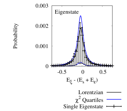
Figure 7: Average squared coefficients $\langle|c_{s,\epsilon}^{(\xi)}|^{2}\rangle$ for a single eigenstate follow the Lorentzian distribution of Eq. 65. Error bars show the first and third quartiles of the distribution of $|c_{s,\epsilon}^{(\xi)}|^{2}$ in each data point. The quartiles of the coefficient distributions are in good agreement with the quartiles of the single degree of freedom $\chi^{2}$ distribution with the Lorentzian mean, shown in blue.

Fig. 7 shows an example of a single eigenstate calculated by exact diagonalization of our Hamiltonian. In the figure, we averaged squared-coefficients $|c_{s,\epsilon}^{(\xi)}|^{2}$ with nearby energies $E_{s}+E_{\epsilon}$ to get the averages $\langle|c_{s,\epsilon}^{(\xi)}|^{2}\rangle$ shown as data points in the figure. The averages $\langle|c_{s,\epsilon}^{(\xi)}|^{2}\rangle$ represent the average probability of measuring an $|s\rangle|\epsilon\rangle$ state of energy $E_{s}+E_{\epsilon}$ when in the eigenstate $|\xi\rangle$ of energy $E_{\xi}$. The averages are very well described by the Lorentzian $\langle|c_{s,\epsilon}^{(\xi)}|^{2}\rangle\approx L_{\xi}(E_{s}+E_{\epsilon})$, with $L_{\xi}$ from Eq. 65.

The asymmetric error bars in the figure show the first and third quartiles of the distribution of squared coefficients $|c_{s,\epsilon}^{(\xi)}|^{2}$ for each data-point average $\langle|c_{s,\epsilon}^{(\xi)}|^{2}\rangle$. The quartiles are in good agreement with the quartiles of a single degree of freedom $\chi^{2}$ distribution with mean $L_{\xi}(E_{s}+E_{\epsilon})$. The $\chi^{2}$ distribution describes a sum of squared random Gaussian variates. This suggests that the $g_{s,\epsilon}^{(\xi)}$ in Eq. 64 behave as random standard Gaussian variates, so that the squared coefficients $|c_{s,\epsilon}^{(\xi)}|^{2}$ follow the $\chi^{2}$ distribution with mean $L_{\xi}$. To check this, in Fig. 8 we plot the distribution of the $g_{s,\epsilon}^{(\xi)}=c_{s,\epsilon}^{(\xi)}/\sqrt{L_{\xi}(E_{s}+E_{\epsilon})}$, where they are indeed seen to follow a standard Gaussian distribution

$$p(g_{s,\epsilon}^{(\xi)})=p\left(\frac{c_{s,\epsilon}^{(\xi)}}{\sqrt{L_{\xi}(E_{s}+E_{\epsilon})}}\right)\sim e^{-{g_{s,\epsilon}^{(\xi)}}^{2}/2}.$$ (67)

The Gaussian variations for $g_{s,\epsilon}^{(\xi)}$ in Eq. 67 explain the $\chi^{2}$ distributed quartiles in Fig. 7, and are consistent the work of Deutsch [14, 15] and Nation and Porras [16]. We have thus arrived at the description of the eigenstates in Eq. 64, with the Lorentzian $L_{\xi}$ of Eq. 65 and the random variations $g_{s,\epsilon}^{(\xi)}$ of Eq. 67.

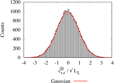
Figure 8: Histogram counts of coefficient variations for an eigenstate. The variations $g_{s,\epsilon}^{(\xi)}=c_{s,\epsilon}^{(\xi)}/\sqrt{L_{\xi}}$ in the single eigenstate coefficients of Eq. 64 follow the standard Gaussian distribution of Eq. 67.

The Gaussian fluctuations in the basis state probabilities of Eq. 64 are related to the random structure of the interaction, as discussed by Deutsch [14, 15]. They also have a connection to the random states considered in the “typicality” approaches to quantum statistical mechanics [20, 21, 22, 23, 24, 25, 26, 27]. These approaches seek to rationalize thermalization behavior by analyzing the statistics of random states. An unbiased sampling of random states is accomplished by taking coefficients as random Gaussian variates [20], similar to our Eq. 67. Here, the eigenstates can be thought of as random or “typical” states within their Lorentzian windows, as seen in Fig. 8.

B.2 Time evolution of an $|s\rangle|\epsilon\rangle$ initial state

Our goal in this section is to understand the behavior of a very simple time-dependent state, from Eq. 26 of the main text, that begins in single zero-order basis state

$$|\Psi_{s,\epsilon}(t)\rangle=e^{-i\hat{H}t}|s\rangle|\epsilon\rangle=\sum_{s^{\prime},\epsilon^{\prime}}c_{s^{\prime},\epsilon^{\prime}}(t)|s^{\prime}\rangle|\epsilon^{\prime}\rangle.$$ (68)

Our analysis will give the Lorentzian behavior for the time-evolved state $|\Psi_{s,\epsilon}(t)\rangle$ seen in Fig. 3 and Eqs. 27-29 of the main text. We now briefly describe these results, repeated here in Eqs. 69-71, before going into the mathematical details of how we obtain the results in the remainder of the section.

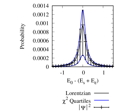
Figure 9: Average squared coefficients $\langle|c_{s^{\prime},\epsilon^{\prime}}(t)|^{2}\rangle$ for a time-evolved $|s\rangle|\epsilon\rangle$ state of Eq. 68 follow a Lorentzian distribution with twice the width of the eigenstates. Error bars show the first and third quartiles of the distribution of the individual $|c_{s^{\prime},\epsilon^{\prime}}(t)|^{2}$ in each data point. The quartiles of the coefficient distributions are in good agreement with the quartiles of the two degree of freedom $\chi^{2}$ distribution scaled by half the Lorentzian weight, shown in blue.

Fig. 9 shows an example of average squared coefficients $\langle|c_{s^{\prime},\epsilon^{\prime}}(t)|^{2}\rangle$ for a time-evolved $|s\rangle|\epsilon\rangle$ state of the type in Eq. 68, at a time $t$ at equilibrium (the results are similar for other choices of $t$). The state is the same as in Fig. 3 of the main text. The average squared coefficients $\langle|c_{s,\epsilon}|^{2}\rangle$ for the state follow a Lorentzian distribution with twice the width of the eigenstate seen previously in Fig. 7; note the energy range in Fig. 9 is doubled relative to Fig. 7. The equilibrated state of Eq. 68 can be expressed in the Lorentzian form from Eqs. 27-29 of the main text,

$$|\Psi_{s,\epsilon}(t)\rangle\approx\sum_{s^{\prime},\epsilon^{\prime}}\tilde{g}_{s^{\prime},\epsilon^{\prime}}\sqrt{L^{(s,\epsilon)}_{f}}|s^{\prime}\rangle|\epsilon^{\prime}\rangle,$$ (69)

where the $\tilde{g}_{s^{\prime},\epsilon^{\prime}}$ are random complex fluctuations and $L^{(s,\epsilon)}_{f}$ is a Lorentzian centered at the initial $|s\rangle|\epsilon\rangle$ energy $E_{0}=E_{s}+E_{\epsilon}$,

$$L^{(s,\epsilon)}_{f}(E_{s^{\prime}}+E_{\epsilon^{\prime}})=\frac{1}{\pi}\frac{\gamma_{f}/\rho_{f}}{(E_{s^{\prime}}+E_{\epsilon^{\prime}}-E_{0})^{2}+\gamma_{f}^{2}},$$ (70)

with half-width at half-max

$$\gamma_{f}=2\pi k^{2}\rho_{f},$$ (71)

where $\rho_{f}=\rho(E_{0})$ is the total density of system-environment states at $E_{0}$. The Lorentzian is similar to the eigenstate Lorentzian in Eqs. 65 and 66, except that the eigenstate energy has been replaced with the initial state energy $E_{0}=E_{s}+E_{\epsilon}$, the width is doubled to $2\pi k^{2}\rho_{f}$, and there is no median energy parameter $\Delta E_{0}$.

The error bars in Fig. 9 show the quartiles of the distributions of squared coefficients for each data point, they are in very good agreement with the quartiles of a two degree of freedom $\chi^{2}$ distribution scaled by 1/2 the Lorentzian. This will be related to the structure of the random deviation terms $\tilde{g}_{s^{\prime},\epsilon^{\prime}}$ in Eq. 69, which we will find to follow statistics where their real and imaginary parts can be treated as random Gaussian variates, as in Eq. 24 of the main text. We now discuss how we obtain these results mathematically.

B.2.1 Average Lorentzian Distribution $\bm{L_{s,\epsilon}}$ for the time-evolved $\bm{|s\rangle|\epsilon\rangle}$ state

To derive the average Lorentzian behavior of Eq. 69, we begin by calculating the average equilibrium state distribution for the time-evolving state of Eq. 68. The average equilibrium behavior is given by the long-time average of the density operator

$$\langle\hat{\rho}_{s,\epsilon}\rangle_{t\to\infty}=\big{\langle}|\Psi_{s,\epsilon}(t)\rangle\langle\Psi_{s,\epsilon}(t)|\big{\rangle}_{t\to\infty}=\sum_{\xi,\xi^{\prime}}c^{(s,\epsilon)}_{\xi}{c^{(s,\epsilon)}_{\xi^{\prime}}}^{*}\big{\langle}e^{-i(E_{\xi}-E_{\xi^{\prime}})t}\big{\rangle}_{t\to\infty}|\xi\rangle\langle\xi^{\prime}|,$$ (72)

where the time-averages are $\langle x\rangle_{t\to\infty}\equiv\lim_{t\to\infty}(1/t)\int_{0}^{t}d\tau x(\tau)$ and the coefficients are given by Eq. 64 with $c_{\xi}^{(s,\epsilon)}=\langle\xi|s\rangle|\epsilon\rangle=\ {c_{s,\epsilon}^{(\xi)}}^{*}$. The energy eigenvalues are non-degenerate since there are no symmetries in the random matrix model, so the cross terms average to zero and

$$\langle\hat{\rho}_{s,\epsilon}\rangle_{t\to\infty}=\sum_{\xi}|c^{(s,\epsilon)}_{\xi}|^{2}|\xi\rangle\langle\xi|=\sum_{\xi}|g_{s,\epsilon}^{(\xi)}|^{2}L_{\xi}(E_{0})|\xi\rangle\langle\xi|,$$ (73)

where the last equality has replaced the $|c^{(s,\epsilon)}_{\xi}|^{2}$ with the expressions from Eq. 64, with the initial state energy $E_{0}=E_{s}+E_{\epsilon}$.

We are interested in the distribution of the time-average density operator of Eq. 73 in the $\{|s\rangle|\epsilon\rangle\}$ basis, where the diagonal elements are $\langle s^{\prime}|\langle\epsilon^{\prime}|\langle\hat{\rho}_{s,\epsilon}\rangle_{t\to\infty}|\epsilon^{\prime}\rangle|s^{\prime}\rangle$. Using the form of the eigenstates in Eqs. 63 and 64 the diagonal elements of the density operator in the zero-order basis are

$$\langle s^{\prime}|\langle\epsilon^{\prime}|\langle\hat{\rho}_{s,\epsilon}\rangle_{t\to\infty}|\epsilon^{\prime}\rangle|s^{\prime}\rangle\approx\sum_{\xi}|g_{s,\epsilon}^{(\xi)}|^{2}|g_{s^{\prime},\epsilon^{\prime}}^{(\xi)}|^{2}L_{\xi}(E_{0})L_{\xi}(E_{s^{\prime}}+E_{\epsilon^{\prime}}).$$ (74)

We assume that the Gaussian variates are statistically independent from the Lorentzian factors so we can simply approximate them with their mean values $\langle|g_{s,\epsilon}^{(\xi)}|^{2}\rangle=\langle|g_{s^{\prime},\epsilon^{\prime}}^{(\xi)}|^{2}\rangle=1$ for all values of the indices $\xi,s,\epsilon,s^{\prime},\epsilon^{\prime}$. With this approximation

$$\langle s^{\prime}|\langle\epsilon^{\prime}|\langle\hat{\rho}_{s,\epsilon}\rangle_{t\to\infty}|\epsilon^{\prime}\rangle|s^{\prime}\rangle\approx\sum_{\xi}L_{\xi}(E_{0})L_{\xi}(E_{s^{\prime}}+E_{\epsilon^{\prime}}).$$ (75)

We will now make two approximations to greatly simplify this sum, resulting ultimately in a single Lorentzian factor. The first approximation uses a single density of states $\rho(E_{\xi})=\rho(E_{0})$ evaluated at the initial state energy $E_{0}=E_{s}+E_{\epsilon}$ instead of the variable eigenstate energy $E_{\xi}$. This approximation is reasonable since most of the sum comes from eigenstates with eigenenergies $E_{\xi}\approx E_{0}$ where the Lorentzians are near their maxima in Eq. 65. The second approximation is to replace the sum by an integral over all energies, which is reasonable since the discrete energy level spacings are small. With these approximations Eq. 75 becomes

$$\langle s^{\prime}|\langle\epsilon^{\prime}|\langle\hat{\rho}_{s,\epsilon}\rangle_{t\to\infty}|\epsilon^{\prime}\rangle|s^{\prime}\rangle$$

$$\approx\frac{1}{\pi^{2}\rho}\int_{-\infty}^{\infty}dE_{\xi}\frac{\pi k^{2}\rho}{(E_{0}+\Delta E_{0}-E_{\xi})^{2}+(\pi k^{2}\rho)^{2}}\frac{\pi k^{2}\rho}{(E_{\xi}-E_{s^{\prime}}-E_{\epsilon^{\prime}}-\Delta E_{0})^{2}+(\pi k^{2}\rho)^{2}},$$ (76)

where $\rho=\rho(E_{0})$. There is an additional factor of the density of states $\rho(E_{0})$ in the integrand of Eq. 76 in comparison to the summands in Eq. 75 since there are $\rho dE_{\xi}$ summands within each interval $dE_{\xi}$ of the integration. The integral gives the convolution of two Lorentzians. We evaluated the integral using Mathematica, the result is a Lorentzian with twice the half-width at half-max and a central energy at $E_{s^{\prime}}+E_{\epsilon^{\prime}}=E_{0}$,

$$\langle s^{\prime}|\langle\epsilon^{\prime}|\langle\hat{\rho}_{s,\epsilon}\rangle_{t\to\infty}|\epsilon^{\prime}\rangle|s^{\prime}\rangle\approx\frac{1}{\pi}\frac{2\pi k^{2}}{(E_{s}+E_{\epsilon^{\prime}}-E_{0})^{2}+(2\pi k^{2}\rho)^{2}}.$$ (77)

The relation Eq. 77 gives the average Lorentzian in Eq. 70 and Fig. 9 at the start of this section and in Eqs. 27-29 and Fig. 3 of the main text. It is a Lorentzian centered at the initial state energy $E_{0}=E_{s}+E_{\epsilon}$, with twice the width of the eigenstates, obtained through the convolution of Lorentzians in Eq. 76. This result was also obtained by Deutsch [14, 15] in a similar model. We will now consider the fluctuations about this Lorentzian average, to determine the factors $\tilde{g}_{s^{\prime},\epsilon^{\prime}}$ in Eq. 69.

B.2.2 Fluctuations $\bm{\tilde{g}_{s^{\prime},\epsilon^{\prime}}}$ in the coefficients of the time-evolved $\bm{|s\rangle|\epsilon\rangle}$ state

Now we would like to consider the time-dependent state Eq. 68 as undergoing fluctuations about its equilibrium Lorentzian average from Eq. 77, where the fluctuations are given by the factors $\tilde{g}_{s^{\prime},\epsilon^{\prime}}$ in Eq. 69. We expect that the average squared fluctuation is unity, $\langle|\tilde{g}_{s^{\prime},\epsilon^{\prime}}|^{2}\rangle=1$, so that the $|c_{s^{\prime},\epsilon^{\prime}}(t)|^{2}$ follow the Lorentzian on average. We also expect that the real and imaginary parts of $\tilde{g}_{s^{\prime},\epsilon^{\prime}}$ should contribute equally on average. This implies that the fluctuation term can be expressed as

$$\tilde{g}_{s^{\prime},\epsilon^{\prime}}=\frac{g_{s^{\prime},\epsilon^{\prime}}+ig^{\prime}_{s^{\prime},\epsilon^{\prime}}}{\sqrt{2}},$$ (78)

where the real and imaginary components $g_{s^{\prime},\epsilon^{\prime}}$ and $g^{\prime}_{s^{\prime},\epsilon^{\prime}}$ each have the average squared values $\langle g_{s,\epsilon}^{2}\rangle=\langle{g^{\prime}_{s,\epsilon}}^{2}\rangle=1$, so that $\langle|\tilde{g}_{s^{\prime},\epsilon^{\prime}}|^{2}\rangle=1$.

We examine the real and imaginary components $g_{s^{\prime},\epsilon^{\prime}}$ and $g^{\prime}_{s^{\prime},\epsilon^{\prime}}$ separately, in comparison with the exact coefficients $c_{s^{\prime},\epsilon^{\prime}}(t)$ of Eq. 68. By comparison of Eqs. 68, 69, and 78, we have the following relations for $g_{s^{\prime},\epsilon^{\prime}}$ and $g^{\prime}_{s^{\prime},\epsilon^{\prime}}$,

$$g_{s^{\prime},\epsilon^{\prime}}=\mathrm{Re}\left(\frac{\tilde{g}_{s^{\prime},\epsilon^{\prime}}}{1/\sqrt{2}}\right)=\mathrm{Re}\left(\frac{c_{s^{\prime},\epsilon^{\prime}}(t)}{\sqrt{L^{(s,\epsilon)}_{f}(E_{s^{\prime}}+E_{\epsilon^{\prime}})/2}}\right)$$ (79)

and

$$g_{s^{\prime},\epsilon^{\prime}}^{\prime}=\mathrm{Im}\left(\frac{\tilde{g}_{s^{\prime},\epsilon^{\prime}}}{1/\sqrt{2}}\right)=\mathrm{Im}\left(\frac{c_{s^{\prime},\epsilon^{\prime}}(t)}{\sqrt{L^{(s,\epsilon)}_{f}(E_{s^{\prime}}+E_{\epsilon^{\prime}})/2}}\right).$$ (80)

Fig. 10 shows the distributions of the $g_{s^{\prime},\epsilon^{\prime}}$ and $g_{s^{\prime},\epsilon^{\prime}}^{\prime}$ taken as the right hand sides of Eqs. 79 and 80, at an instant in time $t$ after the $|s\rangle|\epsilon\rangle$ initial state has evolved to equilibrium (the results are similar for other $t$). The $g_{s,\epsilon}$ and $g_{s,\epsilon}^{\prime}$ each follow standard Gaussian distributions, indicating that they are each distributed as random Gaussian variates as in Eq. 67. This is also consistent with the quartile distributions observed previously in Fig. 9; the squared complex fluctuation term $|\tilde{g}_{s^{\prime},\epsilon^{\prime}}|^{2}=(g_{s,\epsilon}^{2}+{g_{s,\epsilon}^{\prime}}^{2})/2$ has the distribution of a sum of two squared random standard Gaussian variates, which gives coefficients that follows the two degree of freedom $\chi^{2}$ distribution scaled by $L^{(s,\epsilon)}_{f}$/2, with the quartiles shown in Fig. 9. Thus, taking $\tilde{g}_{s^{\prime},\epsilon^{\prime}}$ as the sum Eq. 78 with $g_{s,\epsilon}$ and $g^{\prime}_{s,\epsilon}$ as random Gaussian variates is giving an entirely consistent description of our results in Figs. 9 and 10.

This completes our analysis of the time-evolved $|s\rangle|\epsilon\rangle$ state in Eq. 69, where the coefficients $c_{s^{\prime},\epsilon^{\prime}}(t)$ are given in terms of the the Lorentzian averages $\sqrt{L_{f}^{(s,\epsilon)}}$ determined by the analysis of the last section and the complex Gaussian variate fluctuation terms $\tilde{g}_{s^{\prime},\epsilon^{\prime}}$ we have just discussed.

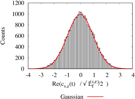
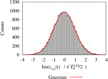
Figure 10: Histogram counts of coefficient variations for a time-evolved $|s\rangle|\epsilon\rangle$ initial state. The real and imaginary parts the variations in Eqs. 79 and 80 each follow a Gaussian distribution.

B.3 Time evolution of a Lorentzian initial state

Now we consider the time evolution of Lorentzian initial states, as in Fig. 2, Eqs. 22-24, and Eqs. 27-29 of the main text. Our goal here is to systematically characterize the equilibration behavior of the Lorentzian initial states, similar to what we did in Section B.2 for the $|s\rangle|\epsilon\rangle$ initial states.

We consider the initial Lorentzian state from Eqs. 22-23 of the main text, repeated here as

$$|\Psi_{L}^{0}\rangle=\sum_{\epsilon}\tilde{g}_{s,\epsilon}\sqrt{L_{0}}|s\rangle|\epsilon\rangle,$$ (81)

where the $\tilde{g}_{s,\epsilon}$ are random complex Gaussian variates as in Eq. 78 and $L_{0}$ is the initial state Lorentzian

$$L_{0}(E_{s}+E_{\epsilon})=\frac{1}{\pi}\frac{\gamma_{0}/\rho_{0}}{(E_{s}+E_{\epsilon}-E_{0})^{2}+\gamma_{0}^{2}},$$ (82)

where $\gamma_{0}$ is the half-width at half-max, $E_{0}$ is the central Lorentzian energy, and $\rho_{0}(E_{0})$ is the density of system-environment states with the system in its initial state $|s\rangle$ at the initial state energy $E_{0}=E_{s}+E_{\epsilon}$. Our goal is to show that this evolves into the final equilibrium state Lorentzian from Eqs. 27-29 of the main text, repeated here as

$$|\Psi_{L}^{f}(t)\rangle=\sum_{s,\epsilon}\tilde{g}_{s,\epsilon}\sqrt{L_{f}}|s\rangle|\epsilon\rangle,$$ (83)

with the final state Lorentzian

$$L_{f}(E_{s}+E_{\epsilon})=\frac{1}{\pi}\frac{\gamma_{f}/\rho_{f}}{(E_{s}+E_{\epsilon}-E_{0})^{2}+\gamma_{f}^{2}},$$ (84)

with half-width at half-max

$$\gamma_{f}=\gamma_{0}+2\pi k^{2}\rho_{f},$$ (85)

where $\rho_{f}=\rho(E_{0})$ is the total density of system-environment zero-order states (when all system levels are accessible at equilibrium).

Fig. 11 shows an initial Lorentzian state of Eq. 81 on the left and a time-evolved version of the same state as in Eq. 83 on the right. The state is the same as in Fig. 2 of the main text. The final state Lorentzian $L_{f}$ is similar to the initial state Lorentzian $L_{0}$ except the width $\gamma_{f}$ is increased by twice the approximate widths of the eigenstates $2\pi k^{2}\rho_{f}$. To rationalize this behavior, we will begin by analyzing the average equilibrium behavior of the time-evolving initial Lorentzian state, then analyze the fluctuations about the average to determine the $\tilde{g}_{s,\epsilon}$. The fluctuations will follow the same type of random Gaussian structure as we had for the time-evolved $|s\rangle|\epsilon\rangle$ states, giving the blue $\chi^{2}$ quartiles in the figure.

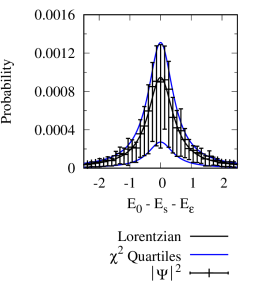
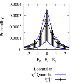
Figure 11: Average squared coefficients $\langle|c_{s^{\prime},\epsilon^{\prime}}(t)|^{2}\rangle$ for a time-evolved Lorentzian initial state of Eq. 81 follows a Lorentzian distribution with increased width (the state is the same as in Fig. 2). Error bars show the first and third quartiles of the distribution of the individual $|c_{s^{\prime},\epsilon^{\prime}}(t)|^{2}$ in each data point. The quartiles of the coefficient distributions are in good agreement with the quartiles of the two degree of freedom $\chi^{2}$ distribution scaled by half the Lorentzian weight, shown in blue.

B.3.1 Average final Lorentzian distribution for the time-evolved Lorentzian initial state

To determine the average final state Lorentzian in Eq. 83, we will calculate the average equilibrium behavior of the time-evolving Lorentzian initial state of Eq. 81, analogous to what we did with the average time-evolving $|s\rangle|\epsilon\rangle$ initial state in Section B.2.1. To begin, express the initial state density operator as

$$\hat{\rho}_{L}^{0}=\hat{\rho}_{L}^{0,\mathrm{diag}}+\hat{\rho}_{L}^{0,\mathrm{coh}},$$ (86)

where $\hat{\rho}_{L}^{0,\mathrm{diag}}$ gives the diagonal component with trace of unity,

$$\hat{\rho}_{L}^{0,\mathrm{diag}}=\sum_{s,\epsilon}|\tilde{g}_{s,\epsilon}|^{2}L_{0}(E_{s}+E_{\epsilon})|s\rangle|\epsilon\rangle\langle\epsilon|\langle s|,$$ (87)

and $\hat{\rho}_{L}^{0,\mathrm{coh}}$ gives the coherences between the $|s\rangle|\epsilon\rangle$ states with trace of zero,

$$\hat{\rho}_{L}^{0,\mathrm{coh}}=\sum_{s,\epsilon\neq s^{\prime},\epsilon^{\prime}}\tilde{g}_{s,\epsilon}\tilde{g}_{s^{\prime},\epsilon^{\prime}}\sqrt{L_{0}(E_{s}+E_{\epsilon})L_{0}(E_{s^{\prime}}+E_{\epsilon^{\prime}})}|s\rangle|\epsilon\rangle\langle\epsilon^{\prime}|\langle s^{\prime}|.$$ (88)

First consider the diagonal component $\hat{\rho}_{L}^{0,\mathrm{diag}}$. Its time average is

$$\langle\hat{\rho}_{L}^{0,\mathrm{diag}}\rangle_{t\to\infty}=\sum_{s,\epsilon}|\tilde{g}_{s,\epsilon}|^{2}L_{0}(E_{s}+E_{\epsilon})\langle\hat{\rho}_{s,\epsilon}\rangle_{t\to\infty},$$ (89)

where $\langle\hat{\rho}_{s,\epsilon}\rangle_{t\to\infty}$ is the time-average of a single $|s\rangle|\epsilon\rangle$ initial state. Using the result for $\langle\hat{\rho}_{s,\epsilon}\rangle_{t\to\infty}$ from Eq. 77, then approximating the sum as a convolution integral analogous to Eq. 76 this gives

$$\langle s^{\prime}|\langle\epsilon^{\prime}|\langle\hat{\rho}_{L}^{0,\mathrm{diag}}\rangle_{t\to\infty}|\epsilon^{\prime}\rangle|s^{\prime}\rangle\approx L_{f}(E_{s^{\prime}}+E_{\epsilon^{\prime}}),$$ (90)

where $L_{f}(E_{s^{\prime}}+E_{\epsilon^{\prime}})$ is the final Lorentzian in Eq. 83. Thus, we have arrived at the final Lorentzian distribution by considering the time-averaged diagonal component of the density operator. We now consider the coherence component of the density operator in Eq. 86.

The coherence component $\langle\hat{\rho}_{L}^{0,\mathrm{coh}}\rangle_{t\to\infty}$ of the time-averaged density operator has trace zero, so it has no contribution to the total probability of the time-averaged state and only serves to give fluctuations about the diagonal component $\langle\hat{\hat{\rho}}_{L}^{0,\mathrm{diag}}\rangle_{t\to\infty}$, with zero average fluctuation per basis state. Based on the average behavior, we will simply approximate time-average of the coherence term as zero

$$\langle s^{\prime}|\langle\epsilon^{\prime}|\langle\hat{\rho}_{L}^{0,\mathrm{coh}}\rangle_{t\to\infty}|\epsilon^{\prime}\rangle|s^{\prime}\rangle\approx 0.$$ (91)

We will find that this approximation works very well to model our results. Similarly, Deutsch treated $\langle\hat{\rho}_{L}^{0,\mathrm{coh}}\rangle_{t\to\infty}$ as negligible when calculating operator expectation values, in Eq. 5.7 of Ref. [15].

From the analysis of this section, the average equilibrium distribution for the initial Lorentzian state of Eq. 81 is

$$\langle s^{\prime}|\langle\epsilon^{\prime}|\langle\hat{\rho}_{L}^{0}\rangle_{t\to\infty}|\epsilon^{\prime}\rangle|s^{\prime}\rangle\approx L_{f}(E_{s^{\prime}}+E_{\epsilon^{\prime}}).$$ (92)

This gives the final average Lorentzian in the time-evolved state of Eq. 83 and Fig. 11. We will now consider the fluctuations about the Lorentzian average, to devise the fluctuation terms $\tilde{g}_{s,\epsilon}$ in the final expression for equilibrium Lorentzian state of Eq. 83.

B.3.2 Fluctuations in the coefficients of the time-evolved Lorentzian state

In this section we analyze the fluctuation terms $\tilde{g}_{s,\epsilon}$ in the expression for the final Lorentzian state of Eq. 83. Following the same reasoning as in Section B.2.2, we assume that the fluctuations $\tilde{g}_{s,\epsilon}$ can be expressed in the form of Eq. 78. We analyze the real and imaginary components $g_{s,\epsilon}$ and $g_{s,\epsilon}^{\prime}$ using relations analogous using Eqs. 79 and 80 but with the final state Lorentzian of Eq. 84,

$$g_{s,\epsilon}=\mathrm{Re}\left(\frac{\tilde{g}_{s,\epsilon}}{1/\sqrt{2}}\right)=\mathrm{Re}\left(\frac{c_{s,\epsilon}(t)}{\sqrt{L_{f}(E_{s}+E_{\epsilon}))/2}}\right)$$ (93)

and

$$g_{s,\epsilon}^{\prime}=\mathrm{Im}\left(\frac{\tilde{g}_{s,\epsilon}}{1/\sqrt{2}}\right)=\mathrm{Im}\left(\frac{c_{s,\epsilon}(t)}{\sqrt{L_{f}(E_{s}+E_{\epsilon})}}\right),$$ (94)

where $c_{s,\epsilon}(t)$ are the exact time-dependent coefficients of the $|s\rangle|\epsilon\rangle$ basis states taken at an instant in time $t$ at equilibrium (the results are similar for other $t$ at equilibrium).

Fig. 12 shows the distribution of the $g_{s,\epsilon}$ and $g_{s,\epsilon}^{\prime}$, taken as the right hand sides of Eqs. 93 and 94. The distributions follow the standard Gaussian distribution, indicating that both $g_{s,\epsilon}$ and $g_{s,\epsilon}^{\prime}$ behave as standard Gaussian variates, analogous to what we saw with the coefficients of the time-evolved $|s\rangle|\epsilon\rangle$ state in Section B.2.2.

In total, we have seen in this section how the time-evolution of an initial Lorentzian state of Eq. 81 gives the final Lorentzian state of Eq. 83, with random complex Gaussian variate fluctuations $\tilde{g}_{s,\epsilon}$ about the final Lorentzian $L_{f}$.

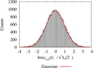
Figure 12: Histogram counts of coefficient variations for a time-evolved Lorentzian initial state. The real and imaginary parts the variations in Eqs. 93 and 94 each follow a Gaussian distribution.

C: Entropy of the Lorentzian

In this section we derive the entropy, Eq. 30 of the main text, for a state with random variations about a Lorentzian, as in the previous sections and in Eqs. 22 and 27 of the main text.

Each of the Lorentzian states has squared coefficients of the approximate form

$$p_{\alpha}=|c_{\alpha}|^{2}\approx|\tilde{g}_{\alpha}|^{2}L_{\alpha}=|\tilde{g}_{\alpha}|^{2}\frac{1}{\pi}\frac{\gamma/\rho}{\Delta E_{\alpha}^{2}+\gamma^{2}},$$ (95)

where $\Delta E_{\alpha}=E_{0}-E_{\alpha}$ is the energy difference between the basis state $|\alpha\rangle=|s\rangle|\epsilon\rangle$ and the initial state energy $E_{0}$, $\tilde{g}_{\alpha}$ is a complex Gaussian variate as in Eqs. 24-25 of the main text, and $\gamma$ is the half-width at half-max of the Lorentzian. Using these coefficient distributions we will calculate the entropy from Eq. 6 of the main text, repeated here as

$$S_{univ}^{Q}=-\sum_{\alpha}p_{\alpha}\ln p_{\alpha}.$$ (96)

Using Eq. 95 the entropy is

$$S^{Q}_{univ}\approx-\sum_{\alpha}|\tilde{g}_{\alpha}|^{2}L_{\alpha}\ln\left(|\tilde{g}_{\alpha}|^{2}L_{\alpha}\right)=-\sum_{\alpha}|g_{\alpha}|^{2}L_{\alpha}\ln\left(L_{\alpha}\right)-\sum_{\alpha}L_{\alpha}|g_{\alpha}|^{2}\ln\left(|g_{\alpha}|^{2}\right)$$ (97)

The $g_{\alpha}$ are statistically independent from the $L_{\alpha}$ by assumption. This suggests replacing the individual $|g_{\alpha}|^{2}$ in the first sum on the right of Eq. 97 with their average value $\langle|g_{\alpha}|^{2}\rangle=1,$

$$\sum_{\alpha}|g_{\alpha}|^{2}L_{\alpha}\ln\left(L_{\alpha}\right)\approx\sum_{\alpha}L_{\alpha}\ln\left(L_{\alpha}\right),$$ (98)

leaving just the entropy of the perfect Lorentzian. For the second sum on the right of Eq. 97 the statistical independence of the $g_{\alpha}$ suggests replacing the $|g_{\alpha}|^{2}\ln\left(|g_{\alpha}|^{2}\right)$ with the average value

$$\sum_{\alpha}L_{\alpha}|g_{\alpha}|^{2}\ln\left(|g_{\alpha}|^{2}\right)\approx\langle|g_{\alpha}|^{2}\ln\left(|g_{\alpha}|^{2}\right)\rangle\sum_{\alpha}L_{\alpha}=\langle|g_{\alpha}|^{2}\ln\left(|g_{\alpha}|^{2}\right)\rangle$$ (99)

where the last equality uses the normalization of the Lorentzian $\sum_{\alpha}L_{\alpha}=1$. In total, Eq. 97 is then approximated as

$$S^{Q}_{univ}\approx-\sum_{\alpha}L_{\alpha}\ln\left(L_{\alpha}\right)-\langle|g_{\alpha}|^{2}\ln\left(|g_{\alpha}|^{2}\right)\rangle$$ (100)

The first term is the entropy of a Lorentzian, while the second term gives the deviation from the perfect Lorentzian entropy due to the random variations in the state.

Now we will evaluate the terms in Eq. 100. The Lorentzian sum in the first term can be approximated as the integral

$$-\sum_{\alpha}L_{\alpha}\ln\left(L_{\alpha}\right)\approx-\int_{-\infty}^{\infty}d(\Delta E_{\alpha})L_{\alpha}(\Delta E_{\alpha})\rho(E_{0})\ln\left(L_{\alpha}(\Delta E_{\alpha})\right)$$ (101)

In the integral approximation, the density of states $\rho$ is factored into the integrand to account for having approximately $\rho d(\Delta E_{\alpha})$ states in the sum that are within each differential interval $d(\Delta E_{\alpha})$ of integration. To simplify the integral, we have approximated the density of states as the constant value at the central energy of the Lorentzian $\rho=\rho(E_{0})$, where the majority of probability in the Lorentzian is located.

To evaluate the integral Eq. 101 we first split it into two separate integrals by factoring $\rho(E_{0})/\rho(E_{0})$ into the logarithm then separating out a term $-\ln\rho(E_{0})$,

$$-\int_{-\infty}^{\infty}d(\Delta E_{\alpha})L_{\alpha}(\Delta E_{\alpha})\rho(E_{0})\ln\left(L_{\alpha}(\Delta E_{\alpha})\right)$$

$$=-\int_{-\infty}^{\infty}d(\Delta E_{\alpha})L_{\alpha}(\Delta E_{\alpha})\rho(E_{0})\ln\left(L_{\alpha}(\Delta E_{\alpha})\rho(E_{0})\right)+\int_{-\infty}^{\infty}d(\Delta E_{\alpha})L_{\alpha}\rho(E_{0})\ln\rho(E_{0})$$ (102)

The first integral on the right of Eq. C: Entropy of the Lorentzian has the well known solution $\ln(4\pi\gamma)$ for the entropy of a continuous Lorentzian distribution, while the second integral is simply $\ln\rho(E_{0})$, since $\rho(E_{0})$ is a constant and $\int_{-\infty}^{\infty}d(\Delta E_{\alpha})\rho(E_{0})L_{\alpha}(\Delta E_{\alpha})=1$ by the normalization of the Lorentzian. Then in total we have

$$-\sum_{\alpha}L_{\alpha}\ln\left(L_{\alpha}\right)\approx\ln(4\pi\gamma\rho(E_{0}))$$ (103)

The final term in Eq. 100 for the average $\langle|g_{\alpha}|^{2}\ln\left(|g_{\alpha}|^{2}\right)\rangle$ is calculated through integration over all the values of $g^{\prime}$ and $g^{\prime\prime}$ with the Gaussian variate probability density $p(g)=(2\pi)^{-1/2}\exp(-g^{2}/2)$,

$$\langle|g_{\alpha}|^{2}\ln\left(|g_{\alpha}|^{2}\right)\rangle=\int_{-\infty}^{\infty}dg^{\prime}\int_{-\infty}^{\infty}dg^{\prime\prime}p(g^{\prime})p(g^{\prime\prime})\frac{g^{\prime 2}+g^{\prime\prime 2}}{2}\ln\frac{g^{\prime 2}+g^{\prime\prime 2}}{2}=g_{0}$$ (104)

where

$$g_{0}=1-\gamma_{EM}$$ (105)

where $\gamma_{EM}=0.577\ 215...$ is the Euler-Mascheroni constant.

Putting Eqs. 103 and 104 into Eq. 100 gives the entropy for the Lorentzian states, in Eq. 30 of the main text,

$$S\approx\ln(4\pi\gamma\rho)-g_{0}.$$ (106)

References

- (1) P. C. Lotshaw and M. E. Kellman. Quantum microcanonical entropy, Boltzmann’s equation, and the second law. J. Phys. Chem. A, 123:831–840, 2019.
- (2) G. L. Barnes, P. C. Lotshaw, and M. E. Kellman. Quantum Thermodynamics, Entropy of the Universe, Free Energy, and the Second Law. ArXiv e-prints, October 2018. ArXiv:1511.06176.
- (3) Phillip C. Lotshaw and Michael E. Kellman. Asymmetric temperature equilibration with heat flow from cold to hot in a quantum thermodynamic system. Phys. Rev. E, 104:054101, Nov 2021.
- (4) P. C. Lotshaw and M. E. Kellman. Simulating quantum thermodynamics of a finite system and bath with variable temperature. Phys. Rev. E, 100:042105, 2019.
- (5) G. L. Barnes and M. E. Kellman. Time dependent quantum thermodynamics of a coupled quantum oscillator system in a small thermal environment. J. Chem. Phys., 139:21410893, 2013.
- (6) M. Esposito and P. Gaspard. Spin relaxation in a complex environment. Phys. Rev. E, 68(5572):066113, 2003.
- (7) L. Silvestri, K. Jacobs, V. Dunjko, and M. Olshanii. Typical, finite baths as a means of exact simulation of open quantum systems. Phys. Rev. E, 89:042131, 2014.
- (8) J. Gemmer, M. Michel, and G. Mahler. Quantum Thermodynamics: Emergence of Thermodynamic Behavior Within Composite Quantum Systems (Second Edition). Lecture Notes in Physics. Springer, 2009.
- (9) D. Jennings and T. Rudolph. Entanglement and the thermodynamic arrow of time. Phys. Rev. E, 81:061130, 2010.
- (10) Hal Tasaki. From quantum dynamics to the canonical distribution: General picture and a rigorous example. Phys. Rev. Lett., 80:1373–1376, Feb 1998.
- (11) J. M. Deutsch. Eigenstate thermalization hypothesis. Rep. Prog. Phys., 91:082001, 2018.
- (12) L. D’Alessio, Y. Kafri, A. Polkovnikov, and M. Rigol. From quantum chaos and eigenstate thermalization to statistical mechanics and thermodynamics. Advances in Physics, 65(3):239–362, 2016.
- (13) A. M. Kaufman, M. E. Tai, A. Lukin, M. Rispoli, R. Schittko, P. M. Preiss, and M. Greiner. Quantum thermalization through entanglement in an isolated many-body system. Science, 353:794–800, 2016.
- (14) J. M. Deutsch. Quantum statistical mechanics in a closed system. Phys. Rev. A, 43:2046–2049, 1991.
- (15) J. M. Deutsch. A closed quantum system giving ergodicity. https://deutsch.physics.ucsc.edu/pdf/quantumstat.pdf. Accessed 3-17-2020.
- (16) C. Nation and D. Porras. Off-diagonal observable elements from random matrix theory: distributions, fluctuations, and eigenstate thermalization. New J. Phys., 20:103003, 2018.
- (17) D. M. Leitner. Quantum ergodicity and energy flow in molecules. Adv. Phys., 64:445–517, 2015.
- (18) D. M. Leitner. Molecules and the eigenstate thermalization hypothesis. Entropy, 20:673, 2018.
- (19) M. Rigol, V. Dunjko, and M. Olshanii. Thermalization and its mechanism for generic isolated quantum systems. Nature, 452:854–858, 2008.
- (20) Sheldon Goldstein, Joel L. Lebowitz, Roderich Tumulka, and Nino Zanghì. Canonical typicality. Phys. Rev. Lett., 96:050403, Feb 2006.
- (21) S. Goldstein, J. L. Lebowitz, C. Mastrodonato, R. Tumulka, and N. Zanghì. Approach to thermal equilibrium of macroscopic quantum systems. Phys. Rev. E, 81:011109, 2010.
- (22) Sheldon Goldstein, Joel L. Lebowitz, Roderich Tumulka, and Nino Zanghì. Long-time behavior of macroscopic quantum systems: Commentary accompanying the english translation of john von neumann’s 1929 article on the quantum ergodic theorem. Eur. Phys. J. H, 35:173–200, 2010.
- (23) P. Reimann. Foundations of statistical mechanics under experimentally realistic conditions. Phys. Rev. Lett., 101:190403, 2008.
- (24) Noah Linden, Sandu Popescu, Anthony J Short, and Andreas Winter. Quantum mechanical evolution towards thermal equilibrium. Phys. Rev. E, 79:061103, 2009.
- (25) Sandu Popescu, Anthony J. Short, and Andreas Winter. Entanglement and the foundations of statistical mechanics. Nature Phys., 2(11):754–758, Nov 2006.
- (26) P. Reimann. Typical fast thermalization processes in closed many-body systems. Nature Comm., 7:10821, 2016.
- (27) S. Goldstein, T. Hara, and H. Tasaki. Extremely quick thermalization in a macroscopic quantum system for a typical nonequilibrium subspace. New J. Phys., 17:045002, 2015.
- (28) J. von Neumann. Proof of the ergodic theorem and the h-theorem in quantum mechanics. Eur. Phys. J. H, 35:201–237, 2010. translated by Roderich Tumulka.
- (29) X. Han and B. Wu. Microscopic diagonal entropy and its connection to basic thermodynamic relations. Phys. Rev. E, 91:062106, 2015.
- (30) A. Polkovnikov. Microscopic diagonal entropy and its connection to basic thermodynamic relations. Ann. of Phys., 326:486–499, 2011.
- (31) S. Kak. Quantum information and entropy. Int. J. Theo. Phys., 46:860–876, 2007.
- (32) A. Stotland, A. A. Pomeransky, E. Bachmat, and D. Cohen. The information entropy of quantum-mechanical states. Europhys. Lett., 67(5):700, 2004.
- (33) M. A. Nielsen and I. L. Chuang. Quantum Computation and Quantum Information. Cambridge, 2000. p. 506.
- (34) Wolfram Math World. https://mathworld.wolfram.com/Euler-MascheroniConstant.html.

References

- [1] P. C. Lotshaw and M. E. Kellman. Quantum microcanonical entropy, Boltzmann’s equation, and the second law. J. Phys. Chem. A, 123:831–840, 2019.
- [2] G. L. Barnes, P. C. Lotshaw, and M. E. Kellman. Quantum Thermodynamics, Entropy of the Universe, Free Energy, and the Second Law. ArXiv e-prints, October 2018. ArXiv:1511.06176.
- [3] Phillip C. Lotshaw and Michael E. Kellman. Asymmetric temperature equilibration with heat flow from cold to hot in a quantum thermodynamic system. Phys. Rev. E, 104:054101, Nov 2021.
- [4] P. C. Lotshaw and M. E. Kellman. Simulating quantum thermodynamics of a finite system and bath with variable temperature. Phys. Rev. E, 100:042105, 2019.
- [5] G. L. Barnes and M. E. Kellman. Time dependent quantum thermodynamics of a coupled quantum oscillator system in a small thermal environment. J. Chem. Phys., 139:21410893, 2013.
- [6] M. Esposito and P. Gaspard. Spin relaxation in a complex environment. Phys. Rev. E, 68(5572):066113, 2003.
- [7] L. Silvestri, K. Jacobs, V. Dunjko, and M. Olshanii. Typical, finite baths as a means of exact simulation of open quantum systems. Phys. Rev. E, 89:042131, 2014.
- [8] J. Gemmer, M. Michel, and G. Mahler. Quantum Thermodynamics: Emergence of Thermodynamic Behavior Within Composite Quantum Systems (Second Edition). Lecture Notes in Physics. Springer, 2009.
- [9] D. Jennings and T. Rudolph. Entanglement and the thermodynamic arrow of time. Phys. Rev. E, 81:061130, 2010.
- [10] Hal Tasaki. From quantum dynamics to the canonical distribution: General picture and a rigorous example. Phys. Rev. Lett., 80:1373–1376, Feb 1998.
- [11] J. M. Deutsch. Eigenstate thermalization hypothesis. Rep. Prog. Phys., 91:082001, 2018.
- [12] L. D’Alessio, Y. Kafri, A. Polkovnikov, and M. Rigol. From quantum chaos and eigenstate thermalization to statistical mechanics and thermodynamics. Advances in Physics, 65(3):239–362, 2016.
- [13] A. M. Kaufman, M. E. Tai, A. Lukin, M. Rispoli, R. Schittko, P. M. Preiss, and M. Greiner. Quantum thermalization through entanglement in an isolated many-body system. Science, 353:794–800, 2016.
- [14] J. M. Deutsch. Quantum statistical mechanics in a closed system. Phys. Rev. A, 43:2046–2049, 1991.
- [15] J. M. Deutsch. A closed quantum system giving ergodicity. https://deutsch.physics.ucsc.edu/pdf/quantumstat.pdf. Accessed 3-17-2020.
- [16] C. Nation and D. Porras. Off-diagonal observable elements from random matrix theory: distributions, fluctuations, and eigenstate thermalization. New J. Phys., 20:103003, 2018.
- [17] D. M. Leitner. Quantum ergodicity and energy flow in molecules. Adv. Phys., 64:445–517, 2015.
- [18] D. M. Leitner. Molecules and the eigenstate thermalization hypothesis. Entropy, 20:673, 2018.
- [19] M. Rigol, V. Dunjko, and M. Olshanii. Thermalization and its mechanism for generic isolated quantum systems. Nature, 452:854–858, 2008.
- [20] Sheldon Goldstein, Joel L. Lebowitz, Roderich Tumulka, and Nino Zanghì. Canonical typicality. Phys. Rev. Lett., 96:050403, Feb 2006.
- [21] S. Goldstein, J. L. Lebowitz, C. Mastrodonato, R. Tumulka, and N. Zanghì. Approach to thermal equilibrium of macroscopic quantum systems. Phys. Rev. E, 81:011109, 2010.
- [22] Sheldon Goldstein, Joel L. Lebowitz, Roderich Tumulka, and Nino Zanghì. Long-time behavior of macroscopic quantum systems: Commentary accompanying the english translation of john von neumann’s 1929 article on the quantum ergodic theorem. Eur. Phys. J. H, 35:173–200, 2010.
- [23] P. Reimann. Foundations of statistical mechanics under experimentally realistic conditions. Phys. Rev. Lett., 101:190403, 2008.
- [24] Noah Linden, Sandu Popescu, Anthony J Short, and Andreas Winter. Quantum mechanical evolution towards thermal equilibrium. Phys. Rev. E, 79:061103, 2009.
- [25] Sandu Popescu, Anthony J. Short, and Andreas Winter. Entanglement and the foundations of statistical mechanics. Nature Phys., 2(11):754–758, Nov 2006.
- [26] P. Reimann. Typical fast thermalization processes in closed many-body systems. Nature Comm., 7:10821, 2016.
- [27] S. Goldstein, T. Hara, and H. Tasaki. Extremely quick thermalization in a macroscopic quantum system for a typical nonequilibrium subspace. New J. Phys., 17:045002, 2015.
- [28] J. von Neumann. Proof of the ergodic theorem and the h-theorem in quantum mechanics. Eur. Phys. J. H, 35:201–237, 2010. translated by Roderich Tumulka.
- [29] X. Han and B. Wu. Microscopic diagonal entropy and its connection to basic thermodynamic relations. Phys. Rev. E, 91:062106, 2015.
- [30] A. Polkovnikov. Microscopic diagonal entropy and its connection to basic thermodynamic relations. Ann. of Phys., 326:486–499, 2011.
- [31] S. Kak. Quantum information and entropy. Int. J. Theo. Phys., 46:860–876, 2007.
- [32] A. Stotland, A. A. Pomeransky, E. Bachmat, and D. Cohen. The information entropy of quantum-mechanical states. Europhys. Lett., 67(5):700, 2004.
- [33] M. A. Nielsen and I. L. Chuang. Quantum Computation and Quantum Information. Cambridge, 2000. p. 506.
- [34] Wolfram Math World. https://mathworld.wolfram.com/Euler-MascheroniConstant.html.