The Time-Averaged Mass-Loss Rates of Red Supergiants As Revealed by their Luminosity Functions in M31 and M33

Abstract

Mass-loss in red supergiants (RSGs) is generally recognized to be episodic, but mass-loss prescriptions fail to reflect this. Evolutionary models show that the total amount of mass lost during this phase determines if these stars evolve to warmer temperatures before undergoing core collapse. The current Geneva evolutionary models mimic episodic mass loss by enhancing the quiescent prescription rates whenever the star’s outer layers exceed the Eddington luminosity by a large factor. This results in a 20$M_{\odot}$ model undergoing significantly more mass loss during the RSG phase than it would have otherwise, but has little effect on models of lower masses. We can test the validity of this approach observationally by measuring the proportion of high-luminosity RSGs to that predicted by the models. To do this, we use our recent luminosity-limited census of RSGs in M31 and M33, making modest improvements to membership, and adopting extinctions based on the recent panchromatic M31 and M33 Hubble surveys. We then compare the proportions of the highest luminosity RSGs found to that predicted by published Geneva models, as well as to a special set of models computed without the enhanced rates. We find good agreement with the models which include the supra-Eddington enhanced mass loss. The models with lower mass-loss rates predict a larger fraction of high-luminosity RSGs than observed, and thus can be ruled out. We also use these improved data to confirm that the upper luminosity limit of RSGs is $\log L/L_{\odot}\sim 5.4$, regardless of metallicity, using our improved data on M31 and M33 plus previous results on the Magellanic Clouds.

1 Introduction

Understanding the evolution of massive stars is important not just in its own right, but also for solving a host of other problems of astrophysical interest, such as modeling the chemical evolution of galaxies, determining the origins of gamma-ray bursts, and interpreting the gravitational wave signatures of merging compact objects. The treatment of convection, the inclusion of magnetic fields, and the distribution of the initial rotation rates all are uncertainties in the construction of massive star evolutionary models. However, Georgy & Ekström (2015) argue that one of the least constrained and most important properties is that of the time-averaged mass-loss rate during the red supergiant (RSG) phase. Such mass loss shortens the lifetime of the RSG phase, and, at high values, results in such stars shedding their hydrogen-rich outer layers and evolving back towards higher temperatures before ending their lives as supernovae (SNe). It also changes the distribution of SN types expected, and possibly even the sort of compact objects left behind, depending upon how much mass is lost during earlier phases.

There is a strong theoretical underpinning to our knowledge of OB stellar winds, where radiation pressure on a multitude of subordinate spectral lines drives the winds (Castor et al. 1975; for reviews, see Puls et al. 2008, Hillier 2009, and Sander 2017). By contrast, there is little understanding of what drives the winds in RSGs. It is often hypothesized that RSG winds are driven by radiation pressure on dust grains. However, there is no clear physical mechanism for lifting the gas above the stellar surface to radii where it is cool enough that dust can form (see, e.g., Puls et al. 2015). Although pulsations are powerful enough to do this in carbon-rich asymptotic giant branch (AGB) stars (Höfner, 2009), they likely are not in RSGs, and turbulence may play an important role, as argued by Josselin & Plez (2007) and Kee et al. (2021). Rau et al. (2018, 2019) has demonstrated the importance of magnetohydrodynamic Alfvén waves in the chromospheres of AGBs in lifting the material; this may also play a role in RSGs. However, what drives the winds in RSGs remains an unsolved problem at present (see, e.g., Wittkowski et al. 2015).

Thus it is not yet possible to calculate the mass-loss rates of RSGs from first principles. Instead, we have long relied purely on empirical prescriptions, such as those given in Reimers (1975), de Jager et al. (1988), and van Loon et al. (2005a). In general these prescriptions provide a formula for the mass-loss rates as a function of luminosity and effective temperature. However, the actual data shows a tremendous scatter (2-3 orders of magnitude) about these simple prescriptions (see, e.g., Figure 1 in Meynet et al. 2015).

One contributing factor to this scatter is that RSGs of different masses and surface gravities can have the same effective temperatures and luminosities: RSGs evolve nearly vertically along a Hayashi track in the Hertzsprung-Russell diagram (HRD), as the luminosity is a steep function of the mean particle mass, which increases as helium is converted into carbon and oxygen. (See also the discussion in Farrell et al. 2020.) Beasor et al. (2020) attempted to get around this issue by measuring the RSG mass-loss rates in clusters; in each cluster, the range of RSG masses will be very small, assuming the cluster formed coevally. Beasor et al. (2020) offer their own mass-loss prescription as a function of initial mass and luminosity, with values that are far lower than that of other studies.

However, there is potentially a much larger problem than taking into account the masses. All of these various mass-loss prescriptions are based upon the measured “instantaneous” mass loss rates of RSGs, not values averaged over the lifetime of the RSG phase. This is of particular concern as RSG mass loss is known to be heavily episodic, particularly at higher luminosities. The van Loon et al. (1999) study suggests that LMC RSGs shed most of their outer layers in short bursts of intense mass-loss. Thus, prescriptions derived from “quiescent” periods tell us little about what is needed from an evolutionary point of view. These periods of high mass loss are likely due to the outer layers of the star exceeding their Eddington luminosity. As explained by Maeder (2009) and Ekström et al. (2012), this unstable situation is created as a result of the high opacity due to variations in the hydrogen ionization beneath the surface of the star. Although these phases have not been observed directly, they can leave evidence in the circumstellar envelopes (see, e.g., Smith et al. 2009 and Moriya et al. 2011). For instance, Decin et al. (2006) has shown that the high luminosity RSG VY CMa underwent a short (100 yr) burst of high mass-loss some 1000 years ago. The 2019/2020 “great dimming” of Betelgeuse was likely caused by “mini-burst” of dust formation (Levesque & Massey, 2020; Montargès et al., 2021; Dupree et al., 2022), underscoring that mass-loss in RSGs has a stochastic nature even outside of the supra-Eddington phase. (For a contrasting view that suggests episodic mass loss is not a common phenomenon among RSGs, see Beasor & Smith 2022.)

Without a full hydrodynamical treatment, there is no precise way to include these mass-loss bursts in evolution models, and one-dimensional models require some approximate way of incorporating both the quiescent and outburst phases. To achieve this, Ekström et al. (2012) (somewhat arbitrarily) adopted a mass-loss rate of $3\times$ that of the quiescent state whenever the calculated luminosity of the RSG envelope exceeds a value of $5\times$ the Eddington luminosity; these are referred to as the “supra-Eddington” periods. (Their quiescent prescription comes from Reimers 1975, 1977 with $\eta=0.5$ for RSGs with masses up to 12$M_{\odot}$, and from their own fit to the data in Figure 3 of Crowther 2001 for more massive RSGs; the latter is roughly a factor of three times larger than the de Jager et al. 1988 rate.) The result of this is a time-averaged mass-loss rate that is a factor of ten higher for a 20$M_{\odot}$ RSG than what would have earlier been assumed using the one of the older prescriptions (Ekström et al., 2012).

We show the effective Geneva time-averaged mass-loss rate as a function of luminosity by the red line in Figure 1, compared to the classic de Jager et al. (1988) prescription shown as the two black lines. We emphasize the mass-loss rates are not constant with the Geneva method because of the supra-Eddington phases. To determine the time-averaged mass-loss rates for each mass track in the Geneva models, we have simply taken the total mass lost during the red supergiant phase in the models and divided by the total time spent as a RSG. Similarly the luminosity we have used is the time-averaged luminosity computed for the corresponding track. We have also indicated the region of mass-loss rates that would be calculated from the Beasor et al. (2020) mass-dependent relation, where we restrict the luminosity ranges to those from the Ekström et al. (2012) models. The figure includes various “instantaneous” measurements of RSG mass-loss rates for comparison. The large range at a given luminosity alluded to above is clear. In adding these points we have excluded AGB stars, as it seems likely that their driving mechanisms are different. (Our referee, Jacco van Loon, notes that the “observed” mass-loss rates may be significantly underestimated for the RSGs with the lowest values, as these are the stars with inefficient dust formation. Thus their actual dust-to-gas ratio is likely lower than what is usually assumed, and hence their mass-loss rates would be underestimated.)

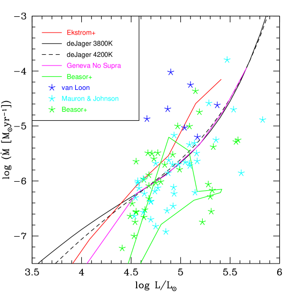
Figure 1: RSG mass-loss prescriptions compared to “instantaneous” observed rates. The red line shows the time-averaged mass-loss rates of RSGs in the models of Ekström et al. (2012), while the lower magenta line comes from the new set of models analyzed here that lack the supra-Eddington mass-loss rates. The two black curves show the mass-loss prescription of de Jager et al. (1988), with the solid line corresponding to an effective temperature of 3800 K, while the dashed line corresponds to 4200 K. The irregular region outlined in green corresponds to the region of mass-loss expected by the new prescription offered by Beasor et al. (2020) computed for the luminosity ranges covered by stars of 12, 15, 20, and 25$M_{\odot}$. Blue points show the mass-loss rates for the subset of RSGs in the van Loon et al. (2005a) study. Cyan points are from Table 1 in Mauron & Josselin (2011). Green points are from Beasor & Davies (2018) and Beasor et al. (2020).

The implications of including the supra-Eddington mass-loss in the evolutionary models are profound. One of the most interesting implications is that it neatly solves the “red supergiant problem” first noted by Smartt et al. (2009). Type II-P supernovae have long been thought to originate from RSGs. However, although RSGs are found with luminosities corresponding to 25-30$M_{\odot}$, Smartt et al. (2009) found that the most luminous of the Type II-P progenitors correspond to masses of only 17-18$M_{\odot}$. The Ekström et al. (2012) calculations show that it is only RSGs above this limit that undergo supra-Eddington mass-loss, suggesting that these stars evolve back to the blue before undergoing core collapse, and hence likely exploding as SNe Type II-L or Ib, having shed most of their hydrogen-rich envelopes during these large mass-loss events.

Meynet et al. (2015) suggested that the direct measurements of RSG mass-loss rates do not preclude their time-averaged values to be even higher, perhaps as much as an additional factor of 10-25$\times$. In contrast, Beasor & Davies (2018) and Beasor et al. (2020) argue that these new evolutionary rates are already too high, although their arguments overlook the short periods of extremely high mass-loss that are expected as the outer layers exceed the Eddington luminosities.

Fortunately, there is an observational test that we can use to address the issue. Meynet et al. (2015) and Georgy & Ekström (2015) note that the RSG luminosity function is quite sensitive to the total amount of mass lost during the RSG stage. This is as expected, in that high mass loss rates will preferentially shorten the lifetimes of the highest luminosity RSGs, depopulating the top end of the RSG luminosity function. Using a limited data set of RSG in M31, Neugent et al. (2020b) demonstrated that the luminosity function was consistent with the Ekström et al. (2012) models that employed the enhanced mass-loss rates during the supra-Eddington phases, but inconsistent with the 10-25$\times$ further enhanced rates considered by Meynet et al. (2015).

Here we reinvestigate the matter using more complete data on the RSG content of M31 and M33, including a comparison to a newly computed set of Geneva models that are similar to those of Ekström et al. (2012) in every way except that the mass-loss rates during the RSG phase have been lowered. This has been done by ignoring any correction for the supra-Eddington phases and adopting the de Jager et al. (1988) relation for the quiescent phase, rather than the slightly higher one derived from the Crowther (2001) data and used in the Ekström et al. (2012) models. The resulting time-averaged mass-loss rate is shown by the magenta line in Figure 1; as expected, it follows the de Jager et al. (1988) relation when $\log L/L_{\odot}>4.5$. Although lower than the (now) standard Geneva rates, they are still much higher than those proposed by Beasor et al. (2020), particularly at larger luminosities and masses, as shown in Figure 1. The primary goal of our study is to see if the observed luminosity functions can successfully be used to rule out lower rates, or if these are, in fact, consistent with the observations. In addition, our improvements to our derivation of the bolometric luminosities of these RSGs allow us to address the long-standing question of the upper luminosity limits of cool supergiants. In Section 2 we detail the construction of the luminosity functions, both theoretical and observational, and in Section 3 we compare the two, as well as discuss the upper luminosity limits of RSGs. Section 4 summarizes our work, and presents our conclusions.

2 Constructing the Luminosity Functions

2.1 Theoretical

In our preliminary study, Neugent et al. (2020b) compared the observed luminosity function of RSGs in M31 to that expected from three sets of Geneva evolutionary models: those computed with the normal mass-loss rates (including the supra-Eddington phases), plus those with 10$\times$ that rate and $25\times$ that rate. Each set included evolutionary tracks that include rotation (initially 40% of the breakup speed), and no rotation. To these sets we now add the “low mass-loss” models, computed similarly to those of Ekström et al. (2012) but without the enhanced supra-Eddington mass-loss and with a pure de Jager et al. (1988) prescription. All models were computed with solar metallicity $Z=0.014$. Further details can be found in Ekström et al. (2012).

Each set of evolutionary models tells us the expected effective temperature and luminosity at each time step for each of the individual mass tracks. What we need, however, is the expected luminosity function for an ensemble of stars. To accomplish this we must carefully interpolate between the discrete mass tracks. In general, the mass tracks represented initial masses of 8$M_{\odot}$, 9$M_{\odot}$, 12$M_{\odot}$, 15$M_{\odot}$, 20$M_{\odot}$, 25$M_{\odot}$, and 32$M_{\odot}$; however, finer-grid tracks were created in the mass range between 8 - 15 $M_{\odot}$ to better model the Cepheid loops. Following, Massey et al. (2021a) and references therein, we assume a constant star-formation rate and a Salpeter (1955) power-law slope of $\Gamma=-1.35$ ($\gamma=-2.35$) for the IMF, where the log of the number of stars between masses $m_{1}$ and $m_{2}$ is simply proportional to $\Gamma\log m\Big{|}_{m_{1}}^{m_{2}}$ (see, e.g., Massey 1998a).

This transformation was accomplished using the Geneva population synthesis code SYnthetic CLusters Isochrones & Stellar Tracks (syclist), described by Georgy et al. (2014). We computed the luminosity functions using a minimum and maximum initial masses of 8$M_{\odot}$ and 30$M_{\odot}$, and restricted the sample to times when the stars had effective temperatures less than or equal to 4200 K. We used 100,000 mass cells (“beams”) in order to avoid quantization issues, and computed locations of stars in the HRD for single-aged populations with ages between 0 and $1.6\times 10^{8}$ yr with time steps of 32,000 years (i.e., 5000 time steps), adopting the $\Gamma=-1.35$ IMF slope. (This time range is much longer than $\sim$30-50 Myr ages of even the lowest mass RSGs.) The final distribution function was then simply summed under the assumption of continuous star formation.

2.2 Observed

To construct the observed luminosity functions, we start with the recent M31 and M33 RSG candidate lists given by Massey et al. (2021b), but modify what is included and the derived luminosities as described in this section. Full details of the determinations of luminosities from near-IR photometry are given in that paper, but we briefly summarize our basic procedure here. The observed $J-K_{s}$ colors were first transformed to the standard Bessell & Brett (1988) $J-K$ system. Next the photometry was corrected for extinction. (Here we improve our treatment of extinction, as described below.) The absolute magnitudes $M_{K}$ were then derived assuming true distance moduli of 24.40 for M31 (i.e., 760 kpc) , and 24.60 for M33 (830 kpc), following van den Bergh (2000) and more recent references. The de-reddened colors were then used to derive temperatures and bolometric corrections to $M_{K}$ using the transformations derived from the MARCS stellar atmospheres (Gustafsson et al., 1975; Plez et al., 1992; Gustafsson et al., 2008).

2.2.1 Completeness

For M31, we restrict our sample to RSGs with galactocentric distances $\rho$ less than 0.75. (The quantity $\rho$ is the de-projected distance within the plane of each galaxy, normalized to the radius at which the surface brightness $\mu_{B}=25.0$ mag arcsec²; see Massey et al. 2021a and Massey et al. 2021b for more details.) Similarly for M33, we restrict our sample to $\rho<1.0$. These limits were chosen for consistency with Massey et al. (2021a), and correspond to the completeness limits of the optical photometry of the Local Group Galaxy Survey (Massey et al., 2006) and the followup spectroscopic survey (Massey et al., 2016).

In Neugent et al. (2020b) we constructed an M31 RSG luminosity function based upon our own Wide Field Camera (WFCAM) $J$ and $K_{s}$ images obtained on the 3.8 m United Kingdom Infrared Telescope (UKIRT) located on Maunakea, Hawai’i. The survey covered 1.26 deg². Subsequently, we used the Andromeda Optical and Infrared Disk Survey data (androids) (Sick et al., 2014) to select RSGs over the entire 5 deg² of M31’s optical disk (Massey et al., 2021b). These data were taken at the Canada France Hawaii Telescope (CFHT), also located on Maunakea, with significantly superior seeing (0$\farcs$5-0$\farcs$6) to those of our UKIRT M31 data (1$\farcs$2-2$\farcs$6).

When we compare the number of RSGs found in the regions of overlapping coverage, we find many more RSGs in the Massey et al. (2021b) CFHT data than in the Neugent et al. (2020b) UKIRT lists. For instance, in the Massey et al. (2021b) CFHT data that corresponds to the UKIRT “Field B” in Neugent et al. (2020b), there are 1904 RSGs identified as more luminous than $\log L/L_{\odot}$=4.0; only 494 (26%) of these were found in the UKIRT survey.

Careful examination revealed that the additional CFHT RSGs were present on the UKIRT images, but had been rejected as detections for several spurious reasons. First, the UKIRT data for each field were obtained during each of two “visits”; i.e., $J$ and $K_{s}$ images were both taken on one night, and then taken again on another night. As described in Neugent et al. (2020b), during each of the visits there were four dithered exposures for $J$ and for $K_{s}$. In order for a detection to be considered valid in Neugent et al. (2020b), it needed to be identified by the Cambridge Astronomy Survey Unit (CASU) pipeline software in both $J$ and $K_{s}$ in the same dither. Furthermore, the star then had to be identified in both visits. Due to the fact that the seeing was invariably worse in one visit than the other, this had the effect of losing some of the fainter stars. Thus the conservative detection requirements, combined with variable (and poor) seeing, accounted for about half of the losses. The explanation for the other half were issues with blending causing the CASU software to fail to notice the object as either a stellar or non-stellar source. In contrast, Massey et al. (2021b) used standard IRAF daofind for object detection and PSF-fitting daophot for object detection and photometry for the CFHT detections. These problems primarily affected the Neugent et al. (2020b) M31 luminosity function below $\log L/L_{\odot}$=4.5; above that, the normalized luminosity function is very similar to the one we derive here using the Massey et al. (2021b) data.

We note that we do not expect these problems to affect the M33 luminosity function we derive from Massey et al. (2021b), despite it also being based upon UKIRT WFCAM imaging. Although those data also relied upon CASU pipeline, they were taken as part of a search for AGB stars by Cioni et al. (2008) under much better seeing conditions (0$\farcs$7-1$\farcs$1) than our own M31 UKIRT data (1$\farcs$2-2$\farcs$6). We also did not impose such draconian restrictions on matching; details are given in Massey et al. (2021b). Finally, M33 poses a far less crowded environment than does M31, as it is seen more face on, with an inclination of 56^∘ (Zaritsky et al., 1989) vs. 77^∘ (de Vaucouleurs et al., 1991).

2.2.2 Revisiting the Extinction Corrections

In determining the extinction corrections for RSGs in M31 and M33, Massey et al. (2021b) adopted a constant reddening for most stars ($A_{V}=0.75$ mag) but applied an additional correction for the brightest RSGs ($K_{s}<14.5$) i.e., $A_{V}=0.75+1.25\times(14.5-K_{s})$ following Neugent et al. (2020b) and Massey et al. (2021b). This correction was based upon spectral fitting of 16 RSGs in M31 in Massey et al. (2009), and is illustrated in Neugent et al. (2020b). In retrospect, there were three problems with that approach. First, the maximum $A_{V}$ of any of the stars included in the Massey et al. (2009) was 2.5 mags, and, through an unfortunate oversight, we extrapolated the relationship to brighter magnitudes, resulting in several unrealistically high extinction corrections. Second, the higher values were defined by only three stars, and the slope and break point ($K_{s}\sim 14.5$) poorly determined. Third, there was no observational evidence that this same relationship should be applied to RSGs in M33. We re-examine the issue here, based upon (1) the additional spectral types now known for RSGs in M31 and M33, and (2) our improved understanding of the average reddenings in these galaxies.

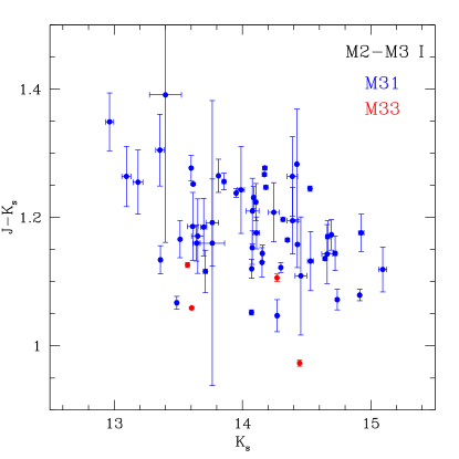
Figure 2: NIR Colors of M2-3 Supergiants. The $J-K_{s}$ colors are shown as a function of $K_{s}$ for known M2-3 I stars in M31 (blue) and M33 (red). There is only a weak correlation between the two for M31. In addition, the M31 M2-3 supergiants are systematically redder than their M33 counterparts, consistent with the average reddening being higher in M31.

We begin our exploration of the reddening issue by examining the colors and previously derived physical properties of a set of RSGs with similar spectral types. There are 54 M2-M3 I stars known in M31 and 4 in M33, which we list in Table 1. Since these stars are of similar spectral type, we expect their intrinsic $J-K_{s}$ colors to be the same. As shown in Figure 2, any variation with magnitude is lost in the scatter. There is a weak linear correlation coefficient for the 54 M31 M2-M3 stars, with a value $r=-0.39$, but with a much smaller slope than suggested by the above relation: From the relationship above, we would have adopted $A_{V}=0.75$ mag at $K_{s}\sim 15$, and $A_{V}=2.0$ mag at $K_{s}\sim 13.5$, given that the color excess $E(J-K)$ will be $A_{V}/5.79$ (Schlegel et al., 1998). Thus, we would have expected stars with $K_{s}\sim 13.5$ to be 0.2 mag redder than than stars with $K_{s}\sim 15$, but that is not what we see. (We will discuss the offset between the M31 and M33 stars further below, but the obvious interpretation is that the reddening is higher in M31.) Thus the extinction correction adopted by Massey et al. (2021b), which was used in our preliminary luminosity function study (Neugent et al., 2020b), no longer appears to be justified. This is further emphasized by the fact that if the color correction based upon the above was applied, then the brighter M2-M3 stars would have temperatures of 4300-4450 K or higher, rather than the 3600-3700 K one would expect given the spectral type (Levesque et al., 2006; Massey et al., 2009). We are sure that there are RSGs in M31 with higher reddening, as found by Massey et al. (2009) (due either to circumstellar material or located in a region of particularly high reddening), but in general the additional extinction correction for the brightest $K_{s}$ stars we previously used is unlikely to be correct.

Here we adopt the following approach. For M31, we make use of the Panchromatic Hubble Andromeda Treasury (PHAT) survey (Dalcanton et al., 2012). Using this comprehensive photometry set, Dalcanton et al. (2015) finds that the average extinction in the disk corresponds to an $A_{V}=1.0$ mag. We can compare this to the extinction found by fitting MARCS RSG models to flux-calibrated spectrophotometry by Massey et al. (2009). For the 16 M31 RSGs in their sample, the median $A_{V}$ value is 1.01 mag; the mean is 1.20 mag, with a 0.6 mag scatter, so this agreement is good.

For M33, the extinctions for multiple regions was measured in a similar manner using the Panchromatic Hubble Andromeda Treasury: Triangulum Extended Region (PHATTER, Williams et al. 2021) data set (Lazzarini et al., 2022). The average roughly corresponds to a value of $A_{V}=0.8$ mag (M. Lazzarini 2022, private communication). Although our recent studies have determined spectral types for many RSGs in M33 (Massey et al. 2021b and references therein), the vast majority of these were obtained using multi-object fiber observations, where the accuracy of the flux calibration is poor. However, we note that the $J-K_{s}$ colors of the M33 M2-3 I stars shown in Figure 2 are less red than their M31 counterparts, consistent with their having lower reddening.

We therefore adopt a constant reddening corresponding to $A_{V}=1.0$ for the M31 RSGs and $A_{V}=0.8$ mag for the M33 RSGs. Since the extinction at $K$ is only 12% of these values (see, e.g., Schlegel et al. 1998), this corresponds to $A_{K}=0.12$ and $A_{K}=0.10$ for M31 and M33, respectively. These corrections are applied after the minor transformation from $K_{s}$ to $K$ as given in Carpenter (2001), i.e., $K=K_{s}+0.044$. Similarly we adopt color excesses of $E(J-K)=0.17$ and $E(J-K)=0.14$ before calculating the temperatures. The equations we used for the color transformations of $J-K_{s}$ to $J-K$, conversion of colors to temperatures, and the calculation of bolometric luminosities can be found in Table 2 of Massey et al. (2021b) and references therein.

We have no doubt that there are RSGs in M31 and M33 with significant additional extinction due to circumstellar material, as is known in the Milky Way and the Magellanic Clouds (see, e.g., Hyland et al. 1969; Elias et al. 1986; van Loon et al. 1999; Stencel et al. 1989; Massey et al. 2005; Levesque et al. 2009), but we believe that adopting a constant reddening is an improvement over past attempts. There is certainly a hint in Figure 2 that the brightest $K_{s}$ stars are slightly redder. This could be investigated further by fitting of well flux-calibrated optical data, and we have plans to do so.

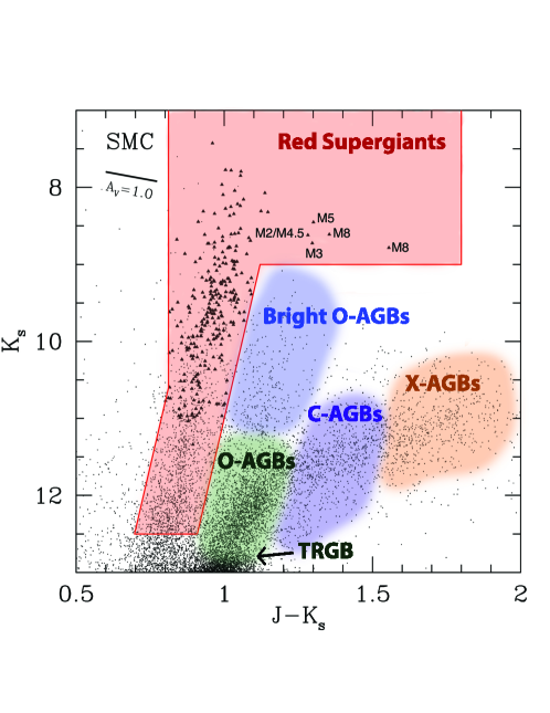
Figure 3: Color-magnitude diagram for the SMC RSGs and AGBs. This figure shows the spectral types for the five SMC stars that are unexpectedly bright and red in the $(J-K_{s},K_{s})$ color-magnitude diagram. The two M8 stars are classified as giants or bright giants by Dorda et al. (2018), although their luminosities suggest otherwise. The star labeled “M5” is HV 11417, the peculiar M supergiant described in detail by Elias et al. (1980). It was suggested as a possible Thorne-Zytkow Object by Beasor et al. (2018), but described as likely Galactic halo object by O’Grady et al. (2020). The M3 I star is HV 2112, the TZO candidate identified by Levesque et al. (2014) (see also Beasor et al. 2018 and O’Grady et al. 2020). The M2/M4.5 I star is [M2002] SMC055188 (Massey, 2002), and identified as a spectrum variable by Levesque et al. (2007). This figure is based upon the data given in Table 5 in Massey et al. (2021a) and is a modified version of their Figure 15.

2.2.3 The Reddest Stars

Another uncertainty we faced in Neugent et al. (2020b) and Massey et al. (2021b) was how to treat a group of stars that are in an unexpected location in the CMDs. Invariably in our previous studies we have found stars in the ($J-K_{s},K_{s}$) plane which are as red as AGB stars, but brighter than we expect AGBs to be found. This is well illustrated in the color-magnitude diagram (CMD) of the Small Magellanic Cloud (SMC) shown in Figure 3. In our studies of the RSG content of the LMC, M31, and M33 (Neugent et al., 2020b, a; Massey et al., 2021b) we assumed that these are heavily reddened RSGs, and determined extinction corrections for each star by projecting back along a reddening line to the median relation between $J-K_{s}$ and $K_{s}$ in our sample. However, by the time we studied RSG population of the SMC (Massey et al., 2021a), our spectroscopy was sufficiently complete to show that most of these stars really were as cool as their $J-K_{s}$ indicated, and were not the result of high reddening. We illustrate this in Figure 3 by indicating the spectral types of these stars.

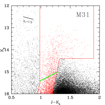
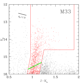
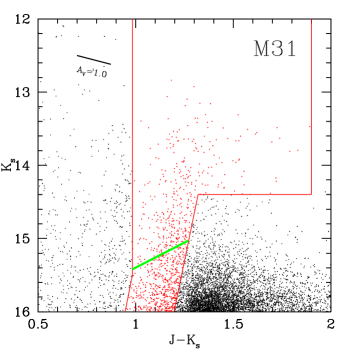
Figure 4: Color-magnitude diagrams for M31 and M33. The top two figures are modified from those in Massey et al. (2021b), with the additional restrictions of $\rho\leq 0.75$ for M31 and $\rho\leq 1.00$ for M33. Foreground stars were removed using DR2 Gaia data in Massey et al. (2021b); we have also removed the additional stars found to be non-members using DR3 here. The third panel, at bottom, shows the CMD for M31 restricting the sample to the regions with lower reddenings. The green diagonal line corresponds to $\log L/L_{\odot}=4.5$. A reddening vector is shown at upper left in each panel. In comparing with the CMD for the SMC shown in Figure 3, recall that there is $\sim$5.5 mag difference in distance modulus.

That said, the CMDs of M31 and M33 given in Figure 4 show some extremely red stars ($J-K_{s}>1.5$). If these stars have only typical reddenings, then their temperatures are 3400 K, corresponding to a spectral subtype a little latter than an M5 supergiant (Levesque et al., 2005). These are surprisingly cool for RSGs, and we suspect that these are primarily super-AGB stars (see, e.g., van Loon et al. 2005a and Goldman et al. 2017). We note that the number of stars eliminated is quite small: 52 stars out of 728 more luminous than $\log L/L_{\odot}$=4.5 for M31, and 8 out of 836 for M33. One of these “too red” M31 objects proved to be a known background galaxy. We have excluded these stars with $J-K_{s}>1.5$ from our discussions of the luminosity function. We note that by doing this we may be excluding some very dusty RSGs, such as the well-known WOH G64 (Elias et al., 1986; van Loon, 1998; Levesque et al., 2009) in the LMC. However, we expect these to be scant in number, and that most of these very red stars will prove to be AGBs.

2.2.4 Removing non-RSGs

There are three potential sources of contamination in the photometry lists of RSG candidates of Massey et al. (2021b): foreground red stars (mostly dwarfs), background galaxies, and globular clusters. Here we remove the residual contaminates before constructing our luminosity functions.

As described in detail by Massey et al. (2021b), for many years the primary way to separate extragalactic RSGs from foreground Galactic red dwarfs was via radial velocity studies, aided by ground-based parallaxes and proper motions for the brightest interlopers (see, e.g., Massey 1998b; Massey et al. 2009; Drout et al. 2012; Massey & Evans 2016.) This all changed with the availability of high precision Gaia astrometry, as was discussed extensively in Aadland et al. (2018). (For an overview of Gaia, see Gaia Collaboration et al. 2016.) The RSG catalogs given in Massey et al. (2021b) were cleaned on the basis of parallax and proper motion data given in Gaia Data Release 2 (Gaia Collaboration et al., 2018). Since then, improved values have become available to the community via Data Release 3 (Gaia Collaboration et al., 2021; Gaia Collaboration, 2022). We used these as follows: First, we used the RSGs designated as members by Massey et al. (2021b) to determine the expected values for the parallaxes and proper motions, as there are zero-point issues that are dependent upon location in the sky. For M31, we find median values of 0.00 mas, +0.012 mas yr^-1, and $-0.077$ mas yr^-1 for the parallax and proper motions in right ascension and declination, respectively, using a sample of 1807 stars after eliminating outliers. For M33, the median values are $-0.04$ mas, +0.059 mas yr^-1, and +0.020 mas yr^-1 using a sample of 1559 stars after eliminating outliers. We used these values to eliminate any previously assumed member if (a) their parallax was $>$$3.5\sigma$ than the median values, or (b) if either of their proper motion values were further from the expected (median) values by 3.5$\sigma$. For $\sigma$, we used the Gaia uncertainties in the relevant values unless they were smaller than the median uncertainty values (0.3 mas for the parallaxes and 0.3 mas yr^-1 for each of the proper motions). If the stated uncertainties were smaller than the median uncertainties, we adopted the median uncertainty as a better representation. This was done in order to avoid the situation of a star with values consistent with membership being rejected simply because the uncertainty was under-estimated.

In addition to the improved astrometric data, we also reviewed the existing radial velocity data for these stars. For M31, such radial velocity information provides a particularly powerful tool, as the galaxy’s systemic velocity is $-300$ km s^-1 and has a rotational velocity of $\sim$240 km s^-1 (Massey et al. 2009 and references therein). Thus, over most of the galaxy the separation is very clean, except for an “alligator jaws” shaped area in the NE section, as shown in Figure 5 of Drout et al. (2009), where the rotational velocity essentially cancels the systemic velocity. For M33 the systemic velocity is $-180$ km s^-1 and the rotational velocity is 74 km s^-1 (Drout et al. 2012 and references therein). To compare with the expected radial velocities as a function of position, we used the relationships between radial velocity and location found by Drout et al. (2009) and Drout et al. (2012) for M31 and M33, respectively. The radial velocities for the M31 RSGs came for Massey & Evans (2016), while the ones for M33 were determined by Drout et al. (2012), supplemented by the project described by Beck & Massey (2017); the actual values of the latter are still in preparation. In all cases the comparison agreed with the conclusions drawn from the Gaia data. The only star eliminated from our list based on published radial velocities (see below) was J004248.37+412506.5, which Drout et al. (2009) designated a foreground object based on its radial velocity. There are no Gaia measurements for the object, but we measured a radial velocity of -45.4 km s^-1, which is highly discrepant with the expected disk velocity at that location, $-216$ km s^-1. The object is now considered a cluster (see, e.g., Fan et al. 2010; Jacoby et al. 2013; Johnson et al. 2015; Caldwell & Romanowsky 2016), known as Bol 129.

Indeed, globular clusters at the distance of M31 and M33 are hard to distinguish from individual stars in many cases, as they are nearly stellar in angular size in typical ground-based seeing. We have therefore vetted our RSG list against catalogs of M31 and M33 clusters. For M31 we used the on-line Version 5 of the Revised Bologna Catalogue of M31 Globular Clusters and Candidates (Galleti et al., 2004), supplemented by the on-line catalog of Hectospec M31 radial velocity of identified objects made available by N. Caldwell (2022, private communication). The Hectospec data also allowed us to identify several additional foreground stars that had lacked Gaia data. As a bonus, both resources contained background galaxies that had been identified on the basis of their radial velocities. Massey et al. (2021b) had eliminated many background galaxies by visual inspection of the images, but of course radial velocities provided a powerful additional means.

Of the 38,856 M31 RSG candidates originally listed by Massey et al. (2021b), the cross-identification with clusters eliminated 406 (1%) spurious objects in M31. The additional vetting using DR3 eliminated another 548 objects, an additional 1.4%, mostly, however, among the brighter objects, as the faint RSG candidates generally lack Gaia data.

There are fewer confirmed clusters in M33 than in M31. We used the updated, on-line version of the Sarajedini & Mancone (2007) catalog available through Vizier. For the clusters not already confirmed from high spatial resolution imaging with HST, Sarajedini & Mancone (2007) used good-seeing (0$\farcs$5) CFHT images to examine objects previously called clusters, and classified them as either clusters, background galaxies, stars, or unknowns. There were 29 matches with the list of 7088 RSG candidates of Massey et al. (2021b), i.e., 0.4%. This fraction is so much lower than that in M31 likely because most of the clusters in M33 are of intermediate age, and not true globular clusters (van den Bergh 2000 and references therein); hence they are not as red, and less likely to be confused with RSGs. We included the “unknowns” in culling process, as their number are scant. Use of the DR3 eliminated another 251 (3.6%).

We also addressed one additional deficiency with our previous methodology. Since our study had excellent astrometry, we had previously cross-matched our lists with Gaia insisting on a match with 1$\farcs$0 using Vizier. However, a careful reading reveals that this tool performs the matching using the original epochs, rather than correcting the coordinates to a common epoch using the measured proper motions. This would result in high proper motion stars falling outside the 1″ search radius, and thus appearing to have no Gaia data. For Gaia, the epoch are 2016.0. For the majority of our M31 data, the epoch is 2007-2009. For M33, the majority of the data have an epoch of 2005. However, both the M31 and M33 lists were supplemented by 2MASS sources, which have an epoch of 1997-2001. Thus the potential contamination by high proper motion stars might well be an issue primarily for the brighter stars. We therefore rechecked the matches for all alledged “non-Gaia” stars in the M31 and M33 catalog using a large (15″) search radius and looked for matches after taking the Gaia-measured proper motions into account. This resulted in eliminating 15 high proper motion stars in M31 and 10 in M33.

2.2.5 Reddening and M31: Redux

As discussed above, we adopt an average extinction for the RSGs in M31 corresponding to $A_{V}=1.0$, and note that this is consistent with the results of spectral fitting by Massey et al. (2009). However, there is another potential concern: RSGs that are so highly hidden by extinction within the disk of M31 that we fail to count them. This could, potentially, affect the luminosity function we adopt, providing a bias against the less luminous stars. Massey et al. (2021b) noted that the percentage of matches between their NIR-constructed catalog of RSGs and the optical Local Group Galaxy Survey (LGGS, Massey et al. 2006, 2016) was much lower for M31 than for M33. They showed that the fraction of matches were strongly correlated with the dust maps of Draine et al. (2014). Thus, in determining the binary frequency of RSGs in M31 and M33, Neugent (2021) restricted her M31 sample to those in regions of low extinction. Similarly, in comparing the relative number of RSGs and Wolf-Rayet (WR) stars as a function of metallicity amongst Local Group galaxies, Massey et al. (2021a) used the same subset of RSGs drawn from the regions of low extinction. We follow the same example here, with the RSGs drawn from regions in M31 where the matches with the LGGS are 50% or greater. This reduces the number of RSGs in our M31 sample from 804 to 409. Applying the same criteria to the broader photometry in Massey et al. (2021b) results in the third CMD shown Figure 4.

One bonus of this additional filtering is that potential contamination of the RSG sample by AGBs is reduced. As shown in Figure 10 of Massey et al. (2021b), the RSG population in M31 is mostly found in the well-known star formation ring, where most of the H i, OB associations, and H$\alpha$ emission is found. By contrast, the much older AGB population is more evenly distributed across the disk, but proportionately higher in the inner regions, where the extinction is higher (see, e.g., Figure 9 in Massey et al. 2021b and Figure 2 in Draine et al. 2014).

3 Results

In the previous section, we described in detail how we computed the predicted RSG luminosity distributions from the evolutionary models. We also give details of the slight adjustments we made in the content and luminosities of the M31 and M33 RSGs identified by Massey et al. (2021b). Now we compare these two to determine if we can truly use the RSG luminosity function to constrain the time-averaged mass-loss rates of RSGs. We finish by using our revised lists to consider the values for the highest luminosities of RSGs in M31 and M33, and compare these values to those of RSGs in the Magellanic Clouds.

Since we have made multiple improvements in the M31 and M33 censuses as described in the previous sections, we are republishing these here as Tables 2 and 3. Following these improvements in the M31 and M33 RSG lists, we have reconsidered both membership and luminosities to our SMC and LMC RSG censuses (given in Massey et al. 2021a and Neugent et al. 2020a, respectively), and reissue our catalogs here as Tables The Time-Averaged Mass-Loss Rates of Red Supergiants As Revealed by their Luminosity Functions in M31 and M33 and The Time-Averaged Mass-Loss Rates of Red Supergiants As Revealed by their Luminosity Functions in M31 and M33, as we will use this information below.

3.1 Comparison with the Evolutionary Models

Neugent et al. (2020b) used M31 to demonstrate that the RSG luminosity functions computed from the solar-metallicity Ekström et al. (2012) evolutionary models were in reasonable agreement with the observations, while those computed from 10$\times$ and 25$\times$ higher RSG mass-loss rates could be ruled out, as they produced luminosity distributions that were much steeper than the observations (i.e., proportionally fewer high luminosity RSGs). Here we address a related question: are the observed luminosity functions also consistent with lower RSG mass-loss rates?

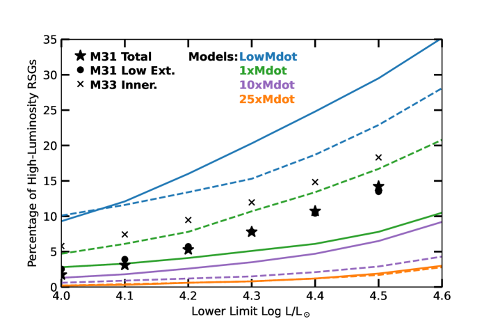
Figure 5: The percentage of the highest luminosity RSGs ($\log L/L_{\odot}\geq 5.0$) observed compared to that predicted by the models with lower luminosity cutoffs from $\log L/L_{\odot}=4.0$ to 4.5. The colored lines show the predictions of the Geneva models; solid lines show the results from models that include rotation (initial value 40% of the breakup speed) while the dashed lines show the results from models without rotation. The points show the observed ratios. The data are most consistent with the normal mass-loss rates (green) from Ekström et al. (2012), which includes the enhanced mass-loss during the supra-Eddington phase. Higher mass loss-rates (purple and orange) predict too few high luminosity RSGs, while removing the enhanced mass-loss during the supra-Eddington phase (blue lines) predict too many high luminosity RSGs.

As discussed earlier, the low and normal mass-loss rate models were computed similarly, with the exception being that the low mass-loss models do not account for the supra-Eddington phases. We expect that the primary effect of removing the enhanced mass-loss will be to increase the numbers of the highest luminosity RSGs, as high mass-loss rates will result in the most luminous RSGs shedding their hydrogen-rich outer layers and evolving back towards higher temperatures before undergoing core collapse. Thus, the percentage of high luminosity RSGs compared to the entire sample should decrease with increasing mass-loss rates. To investigate this, we have computed the percentage of RSGs with high luminosities ($\log L/L_{\odot}\geq 5.0$) RSGs compared to the samples with $\log L/L_{\odot}$$\geq$4.0-4.5. We show the theoretical predictions as colored lines in Figure 5 and give the calculated ratios in Table 6. We see from these that as the assumed RSG mass-loss rates increase, the percentage of high luminosity RSGs indeed drops.

How do these model predictions compare to the observations? For comparison with the output of syclist we count only RSGs with effective temperatures $\leq$4200 K, but this restriction makes negligible difference in the fractions compared to, say, 4300 or 4400 K. We include the measured fractions as discrete points in Figure 5 and tabulate them in Table 6. For M31 we include both the full sample as well as the sample with low extinction. We see that the results are very similar for each of these two samples. A comparison with the model predictions makes it clear that the fractions of high-luminosity RSGs are far more consistent with the mass-loss prescription used in the Ekström et al. (2012) models which includes the enhanced mass-loss during the supra-Eddington phases. For instance, we find that the percentage of high luminosity ($\log L/L_{\odot}\geq 5.0$) RSGs in a sample with $\log L/L_{\odot}\geq 4.2$) is 5.7-7.8%. The low mass-loss models predict a value of 13.4-16.0%, while the normal mass-loss models predict ratios of 4.1-7.8%. Higher mass-loss models predict lower fractions. The same trend is observed for all the luminosity cutoffs, although the M31 points are a little low compared to the models for the $\log L/L_{\odot}=4.0$ and 4.1 points. This suggests to us that the lowest luminosity points suffer some AGB contamination despite the efforts of Massey et al. (2021b) to separate the RSG and AGB populations in the CMDs.

We also include in Table 6 the results for the inner portion ($\rho<0.25$) of M33, where the metallicity is expected to be solar or slightly lower. There we find slightly higher fractions than the normal mass-loss rates predict, but still in far better agreement with those than with lower mass-loss rates. We attribute this small discrepancy to the lower metallicity of the M33 sample compared to that of M31, as lower metallicities will favor longer life-times for the higher luminosities RSGs, which might evolve to WRs were the metallicities higher.

We conclude that the enhanced RSG mass-loss that is included during the surpa-Eddington phases is not only justified from a theoretical point of view, but results in predictions that are a close match to the observations based on mass-limited samples in M31 and M33. Lower mass-loss rates predict too many high-luminosity RSGs compared to observations.

3.2 The Most Luminous RSGs

Besides achieving our primary purpose, we can also use our knowledge of the M31 and M33 luminosity functions to answer another question of astrophysical importance: how does the luminosity limit of RSGs change with metallicity?

In a landmark paper, Humphreys & Davidson (1979) showed although there were hot, massive stars with luminosities as high as $\log L/L_{\odot}\sim 6.3-6.7$ ($M_{\rm bol}=-11$ to $-12$), there were no cooler massive stars with luminosities above $\log L/L_{\odot}=5.7-5.9$ ($M_{\rm bol}=-9.5$ to $-10$), roughly corresponding to 40$M_{\odot}$. This “Humphreys-Davidson limit” decreased with decreasing temperatures for the hottest stars, and then flattened to a constant value for stars cooler than about 15,000 K. This was surprising, as the evolution of massive stars is expected to take place at nearly constant luminosities: what was stopping the most luminous hot stars to evolve to cooler temperatures?

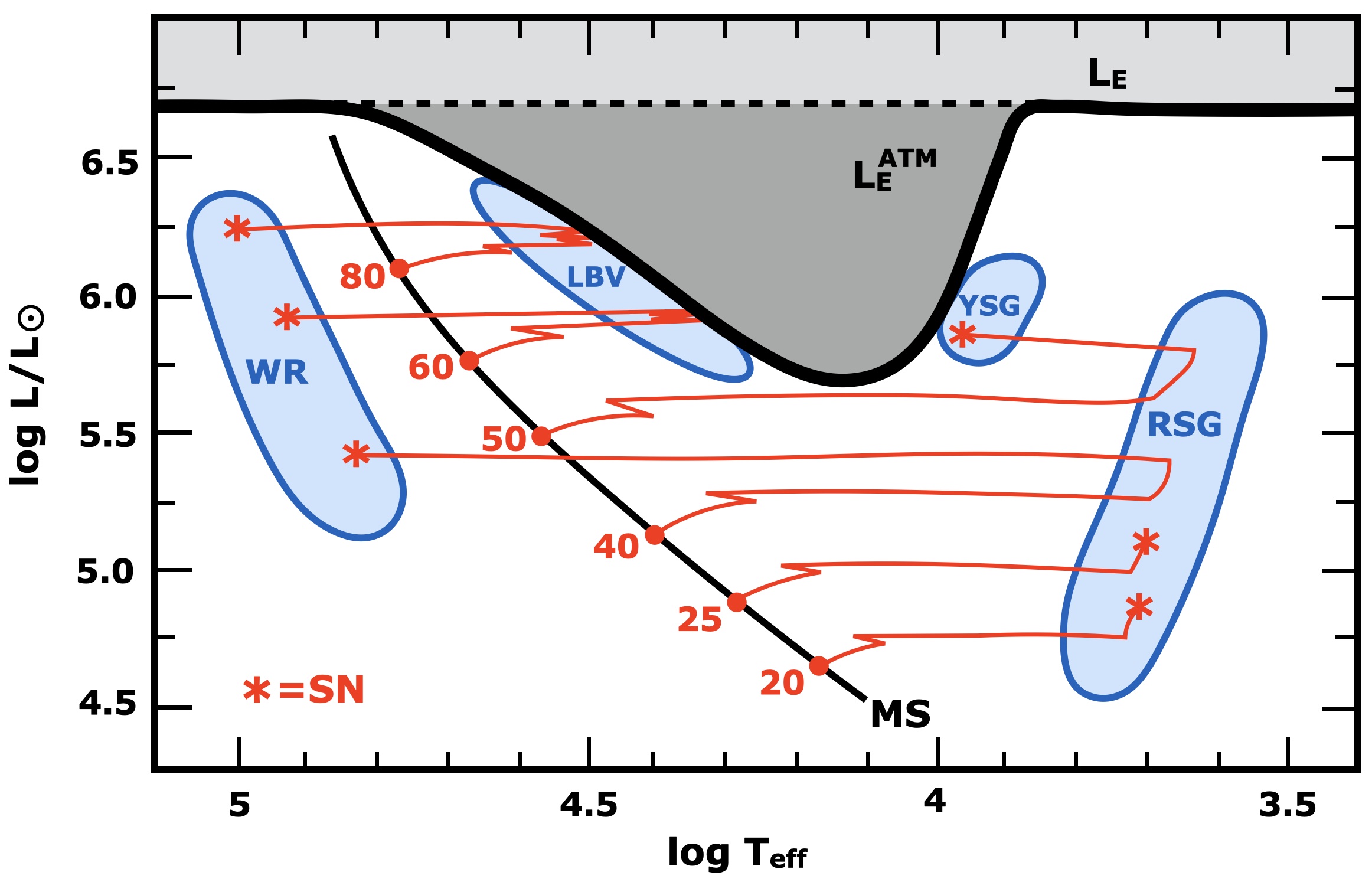
Figure 6: Schematic diagram showing the location of the Eddington trough. Stars evolve from the main-sequence (MS) Higher luminosity (mass) stars encounter the “atmospheric Eddington Limit” (L${}^{\rm ATM}_{E}$) and enter a Luminous Blue Variable (LBV) phase before evolving to Wolf-Rayets (WR). Stars of lower luminosity (mass) evolve to the RSG phase. The most luminous of these will turn around and evolve back to yellow supergiants (YSGs). This figure is based on Figure 22.2 from Lamers & Levesque (2017), and kindly provided to us by Emily Levesque.

The upper luminosity of stars, known as the Eddington limit, is set primarily by the outward force generated by radiation pressure and the inward force of gravity. Classically, the Eddington limit is calculated assuming that electron scattering is the only opacity source (Eddington, 1926). While this is a good approximation for hot, main-sequence stars, line opacity, particularly in the UV, becomes important as a massive star evolves and cools (see, e.g., Lamers & Fitzpatrick 1988). The result is that the upper luminosity limit should be a function of effective temperature, with a minimum value (the so-called “Eddington trough”) reached at an effective temperature of 15,000 K. This is illustrated in Figure 6. Since stellar evolution proceeds at roughly constant luminosity, the upper luminosity of stars cooler than this, such as the yellow and red supergiants, is set by the lowest luminosity of this trough, just as Humphreys & Davidson (1979) found observationally. As stars reach this luminosity limit, high mass-loss rates causes them to lose their extended, convective outer layers, and the stars will shrink and heat up, moving to the left in the H-R diagram, as also shown in Figure 6.

Theoretically, what do we expect to happen to the Humphreys-Davidson limit and the Eddington trough as a function of metallicity? Ulmer & Fitzpatrick (1998) used LTE plane-parallel models to compute the expected dependence of the Eddington trough as a function of metallicity. Line opacity should be increasingly important at higher metallicities, and indeed their calculations show that at M31-like metallicities (1.5$\times$ solar, Sanders et al. 2012) this limit should be at about $\log L/L_{\odot}\sim 5.6$ dex, while at SMC-like metallicities (0.2$\times$solar, Kurt & Dufour 1998; Hunter et al. 2009; Toribio San Cipriano et al. 2017) the limit should be $\sim$6.0 dex. However, further studies have shown that the situation is more complicated than that, and that there is a competing effect that compensates for the metallicity-dependent mass-loss (Higgins & Vink, 2020; Sabhahit et al., 2021). Excess mixing in the superadiabatic outer layers of a star will help keep the star compact, and force evolution back bluewards, limiting the upper luminosity of cooler supergiants. This process is strongest at low metallicities, leading to the expectation that the upper luminosity limit should be around $\log L/L_{\odot}\sim$ 5.5 regardless of luminosity, at least between SMC-like and solar metallicities.

Here we can investigate this afresh using our revised luminosities. In Table 7 we list the most luminous RSGs in M31 and M33, where the latter are divided by their galactrocentric distance within the plane of M33 and have metallicities assigned as done by Neugent & Massey (2011) and references therein. We see that the upper luminosity of RSGs is $\log L/L_{\odot}\sim 5.4$ regardless of metallicities. This result is in excellent agreement with that expected by Higgins & Vink (2020) and Sabhahit et al. (2021), and with the findings by Davies et al. (2018) and Davies & Beasor (2020) that the RSG luminosity limit in the Magellanic Clouds is close to $\log L/L_{\odot}\sim 5.5$. A recent study of the RSG upper luminosity limit in M31 using Spitzer mid-IR photometry by McDonald et al. (2022) found a similar limit.

The Davies et al. (2018) and Davies & Beasor (2020) studies relied upon somewhat older catalogs of Magellanic Cloud RSGs; there have been significant improvements in our knowledge of the RSG content of both galaxies thanks to recent work (e.g., Yang et al. 2020; Neugent et al. 2020a; Massey et al. 2021a). In Table 8 we list the most luminous Magellanic Cloud RSGs, where we have improved the treatment of luminosities from Neugent et al. (2020a) and Massey et al. (2021a) as stated earlier. In agreement with the Davies et al. (2018) study, we find that $\log L/L_{\odot}=5.5$ is a good approximation to the RSG upper luminosity limit, and have extended such studies to the higher metallicity of M31, with results that agree with McDonald et al. (2022) using a sample of RSGs identified independently of the data we use here.

We note that in all of these galaxies, the values of the luminosities could be improved somewhat by modern spectrophotometry and model fitting. However, while this work might shift the results by 0.1 dex or so, it is unlikely to discover any significant metallicity dependence to the upper luminosity limits of RSGs. We also note that these lists of the most luminous RSGs are unlikely to be complete. Dusty RSGs, such as WOH G64 (Elias et al., 1986) and the recently discovered “LMC3” (de Wit et al., 2022) are missing from these lists, as their $J-K$ colors are so large. Nevertheless, the luminosities of these stars are comparable with the upper limits found here: Levesque et al. (2009) finds a value of $\log L/L_{\odot}=5.45\pm 0.05$ for WOH G64, while de Wit et al. (2022) finds $\log L/L_{\odot}=5.47\pm 0.07$.

4 Summary and Conclusions

Mass-loss in RSGs is generally recognized to be episodic (see, e.g., van Loon et al. 1999), but most RSG mass-loss prescriptions used in evolutionary calculations are based upon “instantaneous” measurements that do not take these events into account. Ekström et al. (2012) addressed this problem by increasing the prescribed mass-loss rates by a factor of 3 whenever the model’s luminosity exceeded the Eddington luminosity by a factor of 5. The effect of this was to increase the life-time averaged mass-loss of 20$M_{\odot}$ by a factor of 10; there is little effect expected on RSGs of lower luminosities. This potentially solves the “red supergiant problem” (Smartt et al., 2009), as the increased mass-loss rates would result in higher mass (luminosity) RSGs evolving to higher temperatures before undergoing core collapse.

In this paper we have checked the approach used by Ekström et al. (2012) observationally. The effect of including the enhanced mass-loss rates during the supra-Eddington phases will be to decrease the proportion of the highest luminosity RSGs. For comparison, we have used newly computed Geneva models that differ from the Ekström et al. (2012) models only in not applying a supra-Eddington correction. As expected, they predict a larger fraction of high-luminosity RSGs than the standard models which includes enhanced mass-loss during the supra-Eddington phases. In order to compare the predictions of these models against observations, we have started with the RSG samples in M31 and M33 given by Massey et al. (2021b), and made improvements to both the memberships and luminosities calculations. We have shown that the extinction corrections made by Massey et al. (2021b) were a little too high based upon the inferred temperatures for M2-3 I RSGs. Instead, we have recomputed the luminosities by adopting a uniform reddening for each galaxy based on the average values from the M31 PHAT (Dalcanton et al., 2012, 2015) and M33 PHATTER (Williams et al., 2021; Lazzarini et al., 2022) studies. Given that we are using these $A_{V}$ values to compute corrections to $K$, the differences in luminosities are slight in comparison with Massey et al. (2021b), except for the brightest RSGs where we have argued that Massey et al. (2021b) over-corrected the data. We further cleaned the sample using improved Gaia Data Release 3 results, and also removed known clusters.

We find that the percentage of high-luminosity RSGs in M31 is a good match to the predictions of the Ekström et al. (2012) models. In contrast, the low mass-loss models over-predict the percentage of high-luminosity RSGs. Even lower rates, such as those proposed by Beasor et al. (2020), would require an even higher proportion of high-luminosity RSGs, contrary to what we find. For comparison, we also have shown that the predictions from the Geneva models with 10$\times$ and 25$\times$ enhanced RSG mass-loss rates predict a much lower proportion of high-luminosity RSGs than what is observe. Thus, we find that these much higher rates can also be ruled out, in accordance with the conclusions of Neugent et al. (2020b).

For this study we have relied exclusively on the Geneva models, which do not include the effect of binarity. Yet we know that the binary fraction of RSGs is $\sim$30-40% in M31 and the inner portions of M33 (Neugent, 2021). In our earlier study, Neugent et al. (2020b) showed that there was little difference in the general shape of the RSG luminosity functions derived using the Geneva models and the binary BPASS models of Stanway & Eldridge (2018); the major difference was at the highest luminosities, which we attributed to the BPASS models using the older, low-mass prescriptions. The influence of binarity on RSG luminosities has been further discussed by Zapartas et al. (2021) in the context of the red supergiant problem. They conclude that the expected number of high luminosity RSGs is independent of the inclusion of binary evolution. There are, of course, other questions that we hope to pursue in future work. For instance, how sensitive are the theoretical RSG luminosities to the prescriptions of main-sequence mass-loss?

Finally, we have used our knowledge of these RSG populations to identify the most luminous RSGs in M31 and M33, and we have compared these values to those for RSGs in the SMC and LMC. Our data show that the most luminous RSGs have $\log L/L_{\odot}\sim 5.4$ regardless of metallicity, in accord with the findings of Davies et al. (2018). It has long been supposed that the Humprheys-Davidson limit (Humphreys & Davidson, 1979) should be metallicity dependent (Ulmer & Fitzpatrick, 1998), but more recent work (Higgins & Vink, 2020; Sabhahit et al., 2021) has noted a competing effect: at lowest metallicities excess mixing will reduce the luminosities of the coolest RSGs since these stars will be driven back to warmer temperatures. Our knowledge of the RSG content of these galaxies supports this conclusion.

Table 1: M2-3 Supergiants in M31 and M33

Star	Sp. Type	$K_{s}$	$\sigma_{K_{s}}$	$J-K_{s}$	$\sigma_{J-K_{s}}$
M31
J004312.43+413747.1	M2 I	12.965	0.031	1.349	0.045
J004047.22+404445.5	M2 I	13.096	0.035	1.264	0.047
J004035.08+404522.3	M2 I	13.186	0.038	1.255	0.050
J004125.72+411212.7	M2 I	13.357	0.033	1.305	0.056
J004148.74+410843.0	M2 I	13.361	0.008	1.134	0.022
J004034.74+404459.6	M2.5 I	13.400	0.124	1.391	0.230
J004451.76+420006.0	M2 I	13.488	0.010	1.067	0.010
J004047.82+410936.4	M3 I	13.514	0.001	1.166	0.029
J004447.74+413050.0	M3 I	13.600	0.001	1.277	0.020
J004030.64+404246.2	M3 I	13.612	0.042	1.186	0.053
J004252.78+405627.5	M2 I	13.616	0.001	1.252	0.002
J004120.25+403838.1	M1-2 I	13.643	0.027	1.160	0.028
J004219.25+405116.4	M2 I	13.651	0.047	1.171	0.058
J004501.30+413922.5	M3+ I	13.698	0.024	1.185	0.045
J004415.17+415640.6	M2 I	13.711	0.016	1.116	0.033
J004124.81+411206.1	M2 I	13.765	0.096	1.160	0.222
J004424.94+412322.3	M3 I	13.765	0.050	1.192	0.068
J004118.29+404940.3	M2 I	13.813	0.004	1.265	0.026
J004108.42+410655.3	M3 I	13.856	0.013	1.256	0.013
J004030.92+404329.3	M2 I	13.951	0.006	1.238	0.007
J004447.08+412801.7	M2.5 I	13.989	0.026	1.243	0.068
J004244.52+410345.1	M2 I	14.070	0.003	1.052	0.004
J004517.25+413948.2	M2 I	14.072	0.009	1.120	0.015
J004604.18+415135.4	M2 I	14.076	0.011	1.153	0.026
J004147.27+411537.8	M2 I	14.078	0.050	1.210	0.051
J004120.96+404125.3	M3 I	14.087	0.013	1.231	0.017
J004614.57+421117.4	M3 I	14.104	0.010	1.224	0.029
J004606.25+415018.9	M2 I	14.109	0.024	1.176	0.025
J004552.56+414913.4	M2 I	14.152	0.006	1.130	0.023
J004026.79+404346.4	M2 I	14.155	0.009	1.144	0.013
J004101.02+403506.1	M3 I	14.171	0.002	1.267	0.003
J004558.92+414642.1	M2 I	14.174	0.002	1.277	0.003
J004015.18+405947.7	M3 I	14.182	0.002	1.247	0.003
J004144.65+405446.8	M2 I	14.244	0.042	1.208	0.046
J004449.89+415855.8	M2 I	14.270	0.010	1.047	0.025
J004507.87+413109.0	M3 I	14.299	0.006	1.122	0.008
J004509.73+415950.1	M2 I	14.316	0.002	1.197	0.003
J004211.63+405017.9	M2 I	14.350	0.002	1.165	0.003
J004354.50+411108.3	M3 I	14.389	0.040	1.264	0.062
J004112.38+410918.5	M2 I	14.390	0.042	1.195	0.052
J004122.48+411312.9	M2 I	14.424	0.010	1.283	0.086
J004531.31+415918.3	M2 I	14.428	0.002	1.158	0.036
J004103.55+410750.0	M2 I	14.455	0.046	1.109	0.092
J004213.75+412524.7	M3 I	14.526	0.003	1.245	0.004
J004502.62+414408.3	M2 I	14.531	0.024	1.132	0.046
J004019.15+404150.8	M2 I	14.643	0.002	1.136	0.003
J004133.42+403721.1	M3 I	14.660	0.042	1.143	0.046
J004412.67+413947.8	M2 I	14.664	0.016	1.170	0.025
J004035.16+404105.2	M2 I	14.693	0.003	1.173	0.024
J004623.75+420141.4	M2 I	14.722	0.015	1.144	0.027
J004356.22+413717.6	M2 I	14.738	0.007	1.072	0.016
J004032.89+410155.1	M3 I	14.913	0.007	1.079	0.009
J004359.94+411330.9	M2 I	14.925	0.021	1.176	0.029
J004328.69+410816.4	M2 I	15.093	0.032	1.119	0.035
M33
J013319.13+303642.5	M3 I	13.572	0.001	1.126	0.004
J013258.18+303606.3	M2.5 I	13.604	0.001	1.059	0.002
J013305.17+303119.8	M2-2.5 I	14.269	0.003	1.106	0.006
J013349.83+303224.6	M2.5 I	14.445	0.003	0.973	0.005

Note. — Spectral types and photometry are from Massey et al. 2021b and references therein.

Table 2: RSGs in M31

$\alpha_{2000}$	$\delta_{2000}$	$\rho$	$K_{s}$	$\sigma_{K_{s}}$	$J-K_{s}$	$\sigma_{J-K_{s}}$	#obs	Gaia	Teff	$\log L/L_{\odot}$	LGGS			RV	Exp. RV
											ID	$V$	Type	km s-1	km s-1
00 46 19.482	+41 59 49.66	0.71	16.819	0.012	0.901	0.021	2	2	4250	4.02	$\cdots$	$\cdots$	$\cdots$	$\cdots$	$\cdots$
00 46 20.759	+42 10 01.75	0.71	14.989	0.024	1.211	0.025	2	1	3700	4.58	J004620.78+421001.8	19.99	$\cdots$	$\cdots$	$\cdots$
00 46 20.911	+41 55 45.69	0.75	14.785	0.010	1.156	0.013	3	1	3800	4.69	J004620.92+415545.8	19.76	M1 I	-91.3	-90.6
00 46 23.582	+42 10 12.08	0.72	16.573	0.017	1.071	0.018	2	1	3950	4.03	J004623.60+421012.2	20.74	$\cdots$	$\cdots$	$\cdots$
00 46 23.739	+42 01 41.33	0.72	14.722	0.015	1.144	0.027	2	1	3800	4.73	J004623.75+420141.4	20.00	M2 I	-78.2	-66.6
00 46 25.587	+41 59 11.56	0.74	16.354	0.007	1.096	0.009	2	1	3900	4.10	J004625.59+415911.6	20.67	$\cdots$	$\cdots$	$\cdots$
00 46 25.661	+42 13 21.76	0.74	15.280	0.046	1.178	0.046	2	1	3750	4.48	J004625.67+421322.0	20.14	$\cdots$	$\cdots$	$\cdots$
00 46 25.670	+42 00 46.90	0.73	16.388	0.008	1.111	0.030	2	1	3850	4.08	J004625.69+420046.9	20.72	$\cdots$	$\cdots$	$\cdots$

Note. — Table 2 is published in its entirety in the machine-readable format. A portion is shown here for guidance regarding its form and content.

Table 3: RSGs in M33

$\alpha_{2000}$	$\delta_{2000}$	$\rho$	$K_{s}$	$\sigma_{K_{s}}$	$J-K_{s}$	$\sigma_{J-K_{s}}$	#obs	Gaia	Teff	$\log L/L_{\odot}$	LGGS			RV	Exp. RV
											ID	$V$	Type	km s-1	km s-1
01 32 57.73	+30 12 25.7	0.96	16.757	0.013	0.899	0.021	8	1	4250	4.11	J013257.77+301226.0	20.83	$\cdots$	$\cdots$	$\cdots$
01 32 57.73	+30 43 22.9	0.70	15.688	0.008	0.983	0.013	4	1	4100	4.49	J013257.79+304323.1	19.49	$\cdots$	$\cdots$	$\cdots$
01 32 57.81	+30 35 54.7	0.59	14.453	0.002	1.110	0.004	8	1	3850	4.92	J013257.86+303555.0	19.07	RSG	$\cdots$	$\cdots$
01 32 57.86	+30 24 59.9	0.65	15.604	0.005	1.166	0.009	8	1	3750	4.43	J013257.92+302500.1	20.13	$\cdots$	$\cdots$	$\cdots$
01 32 58.13	+30 36 06.1	0.58	13.604	0.001	1.059	0.002	8	1	3950	5.29	J013258.18+303606.3	18.35	M2.5I	$\cdots$	$\cdots$
01 32 58.14	+30 26 33.6	0.62	16.644	0.012	0.939	0.020	8	1	4150	4.13	$\cdots$	$\cdots$	$\cdots$	$\cdots$	$\cdots$
01 32 58.19	+30 40 05.8	0.63	16.998	0.014	0.825	0.021	12	1	4350	4.05	J013258.25+304006.0	21.60	$\cdots$	$\cdots$	$\cdots$
01 32 58.57	+30 53 53.3	0.97	16.825	0.026	1.007	0.040	2	2	4050	4.03	$\cdots$	$\cdots$	$\cdots$	$\cdots$	$\cdots$

Note. — Table 2 is published in its entirety in the machine-readable format. A portion is shown here for guidance regarding its form and content.

Table 4: RSGs in the SMC

											Spectral Type
2MASS	$\alpha_{\rm J2000}$	$\delta_{\rm J2000}$	$K_{s}$	$\sigma_{Ks}$	$J-K_{s}$	$\sigma_{J-Ks}$	Gaia	$T_{\rm eff}$	$\log L/L_{\odot}$	Type	Ref.	Other ID	Comments
J00450138-7350513	00 45 01.383	-73 50 51.34	11.170	0.019	0.918	0.032	0	4100	4.01	$\cdots$	$\cdots$	$\cdots$	$\cdots$
J00450313-7255156	00 45 03.135	-72 55 15.61	10.314	0.023	0.935	0.033	0	4100	4.35	G8 Ib	5	[GDN2015] SMC079	$\cdots$
J00450456-7305276	00 45 04.566	-73 05 27.69	8.071	0.023	1.137	0.033	0	3750	5.14	M2 I	1	[M2002] SMC 005092	RV var Ref 9
J00450482-7340132	00 45 04.824	-73 40 13.28	12.209	0.027	0.791	0.036	0	4350	3.66	$\cdots$	$\cdots$	$\cdots$	$\cdots$
J00450746-7327417	00 45 07.464	-73 27 41.79	10.300	0.025	1.008	0.035	0	3950	4.31	$\cdots$	$\cdots$	$\cdots$	$\cdots$
J00450758-7358102	00 45 07.581	-73 58 10.21	10.868	0.025	0.923	0.035	0	4100	4.18	G7 Iab-Ib	5	[GDN2015] SMC080	$\cdots$
J00450816-7325382	00 45 08.165	-73 25 38.22	12.131	0.029	0.849	0.038	0	4250	3.66	$\cdots$	$\cdots$	$\cdots$	$\cdots$
J00450831-7254146	00 45 08.312	-72 54 14.64	12.273	0.032	0.920	0.042	0	4100	3.57	$\cdots$	$\cdots$	$\cdots$	$\cdots$

Note. — Table The Time-Averaged Mass-Loss Rates of Red Supergiants As Revealed by their Luminosity Functions in M31 and M33 is published in its entirety in the machine-readable format. A portion is shown here for guidance regarding its form and content.

References. — 1–Levesque et al. (2006); 2–Massey et al. (2007); 3–Levesque et al. (2007); 4–Levesque et al. (2014); 5–Dorda et al. (2018); 6–Massey et al. (2021a); 7–Neugent et al. (2020a); 8–Neugent et al. (2019); 9–Dorda & Patrick (2021); 10–Patrick et al. (2020); 11–Elias et al. (1980); 12–Beasor et al. (2018); 13–Ardeberg & Maurice (1977); 14–Sanduleak (1989).

Table 5: RSGs in the LMC

											Spectral Type
2MASS	$\alpha_{\rm J2000}$	$\delta_{\rm J2000}$	$K_{s}$	$\sigma_{Ks}$	$J-K_{s}$	$\sigma_{J-Ks}$	Gaia	$T_{\rm eff}$	$\log L/L_{\odot}$	Type	Ref.	Other ID
05055608-7032372	05 05 56.082	-70 32 37.29	9.995	0.023	0.997	0.031	0	4050	4.31
05055667-7035238	05 05 56.678	-70 35 23.87	8.114	0.026	1.120	0.033	0	3800	5.00	M4.5I	8	[M2002] LMC 67982
05055720-6858112	05 05 57.206	-68 58 11.23	11.554	0.023	0.944	0.035	0	4150	3.71
05055891-6830314	05 05 58.919	-68 30 31.47	11.599	0.023	0.943	0.033	0	4150	3.70
05055895-7029140	05 05 58.956	-70 29 14.04	8.472	0.023	1.097	0.031	0	3850	4.87	M1I	8	[M2002] LMC 68098
05055950-7048112	05 05 59.506	-70 48 11.24	8.315	0.023	1.168	0.033	0	3750	4.89	M4I	8	[M2002] LMC 68125
05060067-6916283	05 06 00.678	-69 16 28.38	11.512	0.023	0.907	0.031	0	4200	3.75
05060114-6832559	05 06 01.142	-68 32 55.94	11.839	0.026	0.936	0.035	0	4150	3.60

Note. — Table The Time-Averaged Mass-Loss Rates of Red Supergiants As Revealed by their Luminosity Functions in M31 and M33 is published in its entirety in the machine-readable format. A portion is shown here for guidance regarding its form and content.

References. — 1–van Loon et al. (2005b); 2–Hughes & Wood (1990); 3–Heydari-Malayeri et al. (1990); 4–Morgan et al. (1992); 5–Parker et al. (1992); 6–Stock et al. (1976); 7–Oey (1996); 8–Massey & Olsen (2003); 9–Levesque et al. (2006); 10–Cowley & Hartwick (1991); 11–Riaz et al. (2006); 12–Wolf et al. (1987); 13–Reid et al. (1990); 14–Hughes et al. (1991); 15–Reid & Mould (1985); 16–Massey et al. (2000); 17–Dorda et al. (2018); 18–Rousseau et al. (1978); 19–Reid & Parker (2012); 20–Feast (1979); 21–Humphreys (1974); 22–Massey et al. (1989); 23–Sanduleak & Philip (1977); 24–Westerlund et al. (1981).

Table 6: Percentage of High Luminosity RSGs Observed and Predicted

	Percentage of $\log L/L_{\odot}>5.0$ RSGs w.r.t.
	$\log L/L_{\odot}$	$\log L/L_{\odot}$	$\log L/L_{\odot}$	$\log L/L_{\odot}$	$\log L/L_{\odot}$	$\log L/L_{\odot}$
Model/Sample	$\geq 4.0$	$\geq 4.1$	$\geq 4.2$	$\geq 4.3$	$\geq 4.4$	$\geq 4.5$
Model Predictions
Low $\dot{M}$ w/ Rot	9.3	12.0	16.0	20.3	24.8	29.5
Low $\dot{M}$ no Rot	10.1	11.6	13.4	15.3	18.7	22.9
Standard $\dot{M}$ w/ Rot	2.8	3.3	4.1	5.1	6.1	7.8
Standard $\dot{M}$ no Rot	4.7	6.1	7.8	10.7	13.4	16.7
10$\times$ $\dot{M}$ w/Rot	1.3	1.8	2.6	3.5	4.7	6.5
10$\times$ $\dot{M}$ no Rot	0.6	0.9	1.2	1.5	2.1	2.9
25$\times$ $\dot{M}$ w/Rot	0.2	0.3	0.6	0.8	1.2	1.9
25$\times$ $\dot{M}$ no Rot	0.2	0.4	0.6	0.8	1.2	1.7
Observed
M31 (total)	1.7	3.1	5.3	7.8	10.7	14.2
M31 (low ext.)	2.5	3.9	5.7	7.8	10.4	13.5
M33 ($\rho<0.25$)	5.8	7.4	9.5	12.0	14.8	18.3

Table 7: Most Luminous RSGs in M31 and M33

LGGS	Sp.Type	$\rho$	$V$	$K_{s}$	$J-K_{s}$	$T_{\rm eff}$	$\log L/L_{\odot}$
			mag	mag	mag	K
M31 $Z\sim 1.5$
J003951.33+405303.7	$\cdots$	0.75	17.84	12.84	1.18	3750	5.46
J004428.48+415130.9	M1 I	0.47	18.27	13.06	1.16	3800	5.38
J004125.23+411208.9	M0 I	0.48	19.07	12.93	1.30	3500	5.36
J004514.91+413735.0	M1 I	0.61	19.55	12.89	1.34	3450	5.35
J004503.35+413026.3	$\cdots$	0.67	18.82	13.43	0.99	4100	5.33
J004312.43+413747.1	M2 I	0.44	19.36	12.97	1.35	3450	5.32
J004047.22+404445.5	M2 I	0.40	19.33	13.10	1.26	3600	5.31
J004059.50+404542.6	M0 I	0.38	18.71	13.23	1.18	3750	5.31
J004138.35+412320.7	$\cdots$	0.67	18.47	13.39	1.07	3950	5.30
J004148.74+410843.0	M2 I	0.24	19.54	13.36	1.13	3850	5.28
M33 Inner $Z\sim 1.0$
J013336.64+303532.3	RSG	0.18	18.27	13.18	0.99	4100	5.49
J013352.96+303816.0	$\cdots$	0.06	19.42	13.18	1.08	3900	5.45
J013357.08+303817.8	$\cdots$	0.10	18.86	13.61	1.01	4050	5.31
J013335.90+303344.5	$\cdots$	0.22	19.35	13.37	1.24	3650	5.29
J013351.47+303640.3	$\cdots$	0.11	19.92	13.47	1.17	3750	5.28
J013350.84+304403.1	RSG	0.17	19.00	13.56	1.14	3800	5.26
J013403.73+304202.4	RSG	0.14	19.43	13.60	1.19	3750	5.22
J013344.10+304425.1	$\cdots$	0.23	19.15	13.58	1.23	3650	5.21
J013409.63+303907.6	$\cdots$	0.23	20.13	13.36	1.41	3350	5.20
J013338.77+303532.9	$\cdots$	0.16	19.52	13.77	1.13	3850	5.19
M33 Middle $Z\sim 0.5$
J013414.27+303417.7	RSG	0.40	18.34	12.78	1.25	3600	5.52
J013350.62+303230.3	RSG	0.27	18.12	12.98	1.15	3800	5.49
J013358.54+303419.9	OB/RSG?	0.25	17.90	13.21	1.01	4050	5.47
J013412.27+305314.1	RSG	0.47	18.48	13.37	1.12	3850	5.35
J013328.17+304741.5	$\cdots$	0.48	18.27	13.35	1.12	3850	5.35
J013312.35+303033.9	$\cdots$	0.45	18.42	13.51	1.12	3850	5.29
J013309.10+303017.8	RSG	0.48	18.06	13.74	0.98	4100	5.28
J013321.44+304045.4	RSG	0.37	19.17	13.62	1.07	3950	5.28
J013319.13+303642.5	M3 I	0.35	18.72	13.57	1.13	3850	5.27
J013314.31+302952.9	RSG	0.44	19.69	13.47	1.22	3650	5.26
M33 Outer $Z\sim 0.3$
J013241.94+302047.5	$\cdots$	0.84	17.67	13.29	1.06	3950	5.41
J013307.60+304259.0	$\cdots$	0.57	18.35	13.41	1.11	3850	5.34
J013430.75+303218.8	$\cdots$	0.63	19.21	13.38	1.16	3800	5.33
J013303.54+303201.2	RSG	0.52	18.88	13.46	1.11	3850	5.32
J013233.77+302718.8	RSG	0.84	18.32	13.43	1.17	3750	5.30
J013305.48+303138.5	$\cdots$	0.50	18.55	13.44	1.17	3750	5.29
J013423.29+305655.0	RSG	0.61	18.96	13.51	1.12	3850	5.29
J013258.18+303606.3	M2.5 I	0.58	18.35	13.60	1.06	3950	5.29
J013329.47+301848.3	$\cdots$	0.72	18.75	13.55	1.12	3850	5.28
J013312.38+302453.2	RSG	0.56	18.29	13.66	1.06	3950	5.26

Table 8: Most Luminous RSGs in the Magellanic Clouds

2MASS	Sp. Type	$V$	$K_{s}$	$J-K_{s}$	$T_{\rm eff}$	$\log L/L_{\odot}$	Other ID
LMC $Z\sim 0.5$
J05265311-6850002	K/M	12.24	6.62	1.13	3800	5.59	HD 269551. Close OB visual companion.
J05080770-6548486	$\cdots$	$\cdots$	6.63	1.15	3750	5.58	WOH S170
J05294221-6857173	M2	$\cdots$	6.89	1.04	3950	5.53	[M2002] LMC 145013
J05041413-6716143	K/M	11.86	6.78	1.23	3650	5.48	SV* HV 888
J04525366-6655520	K5-M3?	11.14	7.09	0.99	4050	5.47	SP77 21-12
J04443612-7043022	$\cdots$	13.80	6.78	1.27	3550	5.46	SV* HV 12463
J05070565-7032439	M1 I	11.76	7.04	1.08	3900	5.45	SV* HV 5618
J04553485-6926556	$\cdots$	11.76	7.11	1.12	3800	5.40	[M2002] LMC 25320 7″visual double with OB
J05121313-6804555	M0.5 I	11.62	7.32	0.97	4100	5.39	SV* HV 2362
J05352832-6656024	M3 I	12.11	7.26	1.10	3850	5.35	[W60] D44
J05264293-6724326	K/M	11.94	7.38	1.02	4000	5.34	[M2002] LMC 136404
J05302094-6720054	M4 I	12.79	7.45	1.00	4050	5.33	[M2002] LMC 147199
J05355522-6909594	$\cdots$	12.87	7.14	1.41	3300	5.24	OGLE BRIGHT-LMC-LPV-52
J04550307-6929127	$\cdots$	14.44	7.20	1.46	3200	5.19	[M2002] LMC 23095
J05315335-6640432	M3/4 I	12.31	7.57	1.18	3700	5.18	TRM 87
SMC $Z\sim 0.2$
J00510385-7243176	M3 Iab	11.39	7.43	0.96	4050	5.49	[M2002] SMC 018592
J00482702-7312123	M0 I	12.20	7.77	1.00	4000	5.33	[M2002] SMC 010889
J01032764-7252096	K2 Iab	11.85	7.78	1.02	3950	5.32	[M2002] SMC 056389
J01291844-7301590	K:I+B5:I	11.53	7.95	0.91	4150	5.30	[M2002] SMC 83202
J01093824-7320024	K5-M0/M4 I	11.74	7.79	1.06	3900	5.29	[M2002] SMC 069886
J00505609-7215060	M0 I	11.98	7.85	1.05	3900	5.27	[M2002] SMC 018136
J01004151-7210371	K5-M0 I	12.17	7.96	0.99	4000	5.26	[M2002] SMC 049478
J01253885-7321552	K/M	11.84	7.98	1.05	3900	5.22	[M2002] SMC 81961
J01005519-7137529	K0/M4-5 I	11.81	8.04	1.03	3900	5.20	SV* HV 11423
J01043820-7201270	K2-3 I	11.98	8.10	1.00	4000	5.20	[M2002] SMC 059803
J01064766-7216118	K3 Ia	11.87	8.31	0.93	4100	5.15	[M2002] SMC 064663
J00450456-7305276	M2 I	12.90	8.07	1.14	3750	5.14	[M2002] SMC 005092
J00512967-7310442	M0 I	12.33	8.15	1.07	3850	5.14	[M2002] SMC 020133
J00534794-7202095	M2 Ia-Iab	12.43	8.25	1.02	3950	5.13	[S84d] 105-11
J00490034-7259358	K5-M0 I	12.44	8.28	1.00	4000	5.13	[M2002] SMC 12322

Note. — As discussed in the text, extremely dusty RSGs, such as WOH G64 (Elias et al., 1986) and the recently discovered “LMC3” (de Wit et al., 2022), will be missing from these lists, as their $J-K$ colors were so red as to remove them from our RSG lists.

References

- Aadland et al. (2018) Aadland, E., Massey, P., Neugent, K. F., & Drout, M. R. 2018, AJ, 156, 294, doi: 10.3847/1538-3881/aaeb96
- Ardeberg & Maurice (1977) Ardeberg, A., & Maurice, E. 1977, A&AS, 30, 261
- Beasor & Davies (2018) Beasor, E. R., & Davies, B. 2018, MNRAS, 475, 55, doi: 10.1093/mnras/stx3174
- Beasor et al. (2018) Beasor, E. R., Davies, B., Cabrera-Ziri, I., & Hurst, G. 2018, MNRAS, 479, 3101, doi: 10.1093/mnras/sty1744
- Beasor et al. (2020) Beasor, E. R., Davies, B., Smith, N., et al. 2020, MNRAS, 492, 5994, doi: 10.1093/mnras/staa255
- Beasor & Smith (2022) Beasor, E. R., & Smith, N. 2022, ApJ, 933, 41, doi: 10.3847/1538-4357/ac6dcf
- Beck & Massey (2017) Beck, M., & Massey, P. 2017, in American Astronomical Society Meeting Abstracts #229, 433.04
- Bessell & Brett (1988) Bessell, M. S., & Brett, J. M. 1988, PASP, 100, 1134, doi: 10.1086/132281
- Caldwell & Romanowsky (2016) Caldwell, N., & Romanowsky, A. J. 2016, ApJ, 824, 42, doi: 10.3847/0004-637X/824/1/42
- Carpenter (2001) Carpenter, J. M. 2001, AJ, 121, 2851, doi: 10.1086/320383
- Castor et al. (1975) Castor, J. I., Abbott, D. C., & Klein, R. I. 1975, ApJ, 195, 157, doi: 10.1086/153315
- Cioni et al. (2008) Cioni, M. R. L., Irwin, M., Ferguson, A. M. N., et al. 2008, A&A, 487, 131, doi: 10.1051/0004-6361:200809366
- Cowley & Hartwick (1991) Cowley, A. P., & Hartwick, F. D. A. 1991, ApJ, 373, 80, doi: 10.1086/170025
- Crowther (2001) Crowther, P. A. 2001, in The Influence of Binaries on Stellar Population Studies, ed. D. Vanbeveren, Vol. 264 (Dordrecht: Kluwer), 215
- Dalcanton et al. (2012) Dalcanton, J. J., Williams, B. F., Lang, D., et al. 2012, ApJS, 200, 18, doi: 10.1088/0067-0049/200/2/18
- Dalcanton et al. (2015) Dalcanton, J. J., Fouesneau, M., Hogg, D. W., et al. 2015, ApJ, 814, 3, doi: 10.1088/0004-637X/814/1/3
- Davies & Beasor (2018) Davies, B., & Beasor, E. R. 2018, MNRAS, 474, 2116, doi: 10.1093/mnras/stx2734
- Davies & Beasor (2020) —. 2020, MNRAS, 493, 468, doi: 10.1093/mnras/staa174
- Davies et al. (2018) Davies, B., Crowther, P. A., & Beasor, E. R. 2018, MNRAS, 478, 3138, doi: 10.1093/mnras/sty1302
- de Jager et al. (1988) de Jager, C., Nieuwenhuijzen, H., & van der Hucht, K. A. 1988, A&AS, 72, 259
- de Vaucouleurs et al. (1991) de Vaucouleurs, G., de Vaucouleurs, A., Corwin, Herold G., J., et al. 1991, Third Reference Catalogue of Bright Galaxies (Austin: Univ. Texas)
- de Wit et al. (2022) de Wit, S., Bonanos, A. Z., Tramper, F., et al. 2022, arXiv e-prints, arXiv:2209.11239. https://arxiv.org/abs/2209.11239
- Decin et al. (2006) Decin, L., Hony, S., de Koter, A., et al. 2006, A&A, 456, 549, doi: 10.1051/0004-6361:20065230
- Dorda et al. (2018) Dorda, R., Negueruela, I., González-Fernández, C., & Marco, A. 2018, A&A, 618, A137, doi: 10.1051/0004-6361/201833219
- Dorda & Patrick (2021) Dorda, R., & Patrick, L. R. 2021, MNRAS, 502, 4890, doi: 10.1093/mnras/stab303
- Draine et al. (2014) Draine, B. T., Aniano, G., Krause, O., et al. 2014, ApJ, 780, 172, doi: 10.1088/0004-637X/780/2/172
- Drout et al. (2012) Drout, M. R., Massey, P., & Meynet, G. 2012, ApJ, 750, 97, doi: 10.1088/0004-637X/750/2/97
- Drout et al. (2009) Drout, M. R., Massey, P., Meynet, G., Tokarz, S., & Caldwell, N. 2009, ApJ, 703, 441, doi: 10.1088/0004-637X/703/1/441
- Dupree et al. (2022) Dupree, A. K., Strassmeier, K. G., Calderwood, T., et al. 2022, ApJ, 936, 18, doi: 10.3847/1538-4357/ac7853
- Eddington (1926) Eddington, A. S. 1926, The Internal Constitution of the Stars (Cambridge: Cambrdge University Press)
- Ekström et al. (2012) Ekström, S., Georgy, C., Eggenberger, P., et al. 2012, A&A, 537, A146, doi: 10.1051/0004-6361/201117751
- Elias et al. (1980) Elias, J. H., Frogel, J. A., & Humphreys, R. M. 1980, ApJ, 242, L13, doi: 10.1086/183391
- Elias et al. (1986) Elias, J. H., Frogel, J. A., & Schwering, P. B. W. 1986, ApJ, 302, 675, doi: 10.1086/164028
- Fan et al. (2010) Fan, Z., de Grijs, R., & Zhou, X. 2010, ApJ, 725, 200, doi: 10.1088/0004-637X/725/1/200
- Farrell et al. (2020) Farrell, E. J., Groh, J. H., Meynet, G., & Eldridge, J. J. 2020, MNRAS, 494, L53, doi: 10.1093/mnrasl/slaa035
- Feast (1979) Feast, M. W. 1979, MNRAS, 186, 831, doi: 10.1093/mnras/186.4.831
- Gaia Collaboration (2022) Gaia Collaboration. 2022, Gaia DR3 Part 1. Main source, doi: 10.26093/cds/vizier.1355
- Gaia Collaboration et al. (2016) Gaia Collaboration, Prusti, T., de Bruijne, J. H. J., et al. 2016, A&A, 595, A1, doi: 10.1051/0004-6361/201629272
- Gaia Collaboration et al. (2018) Gaia Collaboration, Brown, A. G. A., Vallenari, A., et al. 2018, A&A, 616, A1, doi: 10.1051/0004-6361/201833051
- Gaia Collaboration et al. (2021) —. 2021, A&A, 649, A1, doi: 10.1051/0004-6361/202039657
- Galleti et al. (2004) Galleti, S., Federici, L., Bellazzini, M., Fusi Pecci, F., & Macrina, S. 2004, A&A, 416, 917, doi: 10.1051/0004-6361:20035632
- Georgy & Ekström (2015) Georgy, C., & Ekström, S. 2015, in EAS Publications Series, Vol. 71-72, EAS Publications Series, 41–46
- Georgy et al. (2014) Georgy, C., Granada, A., Ekström, S., et al. 2014, A&A, 566, A21, doi: 10.1051/0004-6361/201423881
- Goldman et al. (2017) Goldman, S. R., van Loon, J. T., Zijlstra, A. A., et al. 2017, MNRAS, 465, 403, doi: 10.1093/mnras/stw2708
- Gustafsson et al. (1975) Gustafsson, B., Bell, R. A., Eriksson, K., & Nordlund, A. 1975, A&A, 42, 407
- Gustafsson et al. (2008) Gustafsson, B., Edvardsson, B., Eriksson, K., et al. 2008, A&A, 486, 951, doi: 10.1051/0004-6361:200809724
- Heydari-Malayeri et al. (1990) Heydari-Malayeri, M., Melnick, J., & van Drom, E. 1990, A&A, 236, L21
- Higgins & Vink (2020) Higgins, E. R., & Vink, J. S. 2020, A&A, 635, A175, doi: 10.1051/0004-6361/201937374
- Hillier (2009) Hillier, D. J. 2009, in American Institute of Physics Conference Series, Vol. 1171, Recent Directions in Astrophysical Quantitative Spectroscopy and Radiation Hydrodynamics, ed. I. Hubeny, J. M. Stone, K. MacGregor, & K. Werner, 111–122
- Höfner (2009) Höfner, S. 2009, in Astronomical Society of the Pacific Conference Series, Vol. 414, Cosmic Dust - Near and Far, ed. T. Henning, E. Grün, & J. Steinacker, 3
- Hughes & Wood (1990) Hughes, S. M. G., & Wood, P. R. 1990, AJ, 99, 784, doi: 10.1086/115374
- Hughes et al. (1991) Hughes, S. M. G., Wood, P. R., & Reid, N. 1991, AJ, 101, 1304, doi: 10.1086/115767
- Humphreys (1974) Humphreys, R. M. 1974, ApJ, 190, L133, doi: 10.1086/181524
- Humphreys & Davidson (1979) Humphreys, R. M., & Davidson, K. 1979, ApJ, 232, 409, doi: 10.1086/157301
- Hunter et al. (2009) Hunter, I., Brott, I., Langer, N., et al. 2009, A&A, 496, 841, doi: 10.1051/0004-6361/200809925
- Hyland et al. (1969) Hyland, A. R., Becklin, E. E., Neugebauer, G., & Wallerstein, G. 1969, ApJ, 158, 619, doi: 10.1086/150224
- Jacoby et al. (2013) Jacoby, G. H., Ciardullo, R., De Marco, O., et al. 2013, ApJ, 769, 10, doi: 10.1088/0004-637X/769/1/10
- Johnson et al. (2015) Johnson, L. C., Seth, A. C., Dalcanton, J. J., et al. 2015, ApJ, 802, 127, doi: 10.1088/0004-637X/802/2/127
- Josselin & Plez (2007) Josselin, E., & Plez, B. 2007, A&A, 469, 671, doi: 10.1051/0004-6361:20066353
- Kee et al. (2021) Kee, N. D., Sundqvist, J. O., Decin, L., de Koter, A., & Sana, H. 2021, A&A, 646, A180, doi: 10.1051/0004-6361/202039224
- Kochanek (2020) Kochanek, C. S. 2020, MNRAS, 493, 4945, doi: 10.1093/mnras/staa605
- Kurt & Dufour (1998) Kurt, C. M., & Dufour, R. J. 1998, in Revista Mexicana de Astronomia y Astrofisica Conference Series, Vol. 7, Revista Mexicana de Astronomia y Astrofisica Conference Series, ed. R. J. Dufour & S. Torres-Peimbert, 202
- Lamers & Fitzpatrick (1988) Lamers, H. J. G. L. M., & Fitzpatrick, E. L. 1988, ApJ, 324, 279, doi: 10.1086/165894
- Lamers & Levesque (2017) Lamers, H. J. G. L. M., & Levesque, E. M. 2017, Understanding Stellar Evolution (Bristol: IOP), doi: 10.1088/978-0-7503-1278-3
- Lazzarini et al. (2022) Lazzarini, M., Williams, B. F., Durbin, M. J., et al. 2022, arXiv e-prints, arXiv:2206.11393. https://arxiv.org/abs/2206.11393
- Levesque & Massey (2020) Levesque, E. M., & Massey, P. 2020, ApJ, 891, L37, doi: 10.3847/2041-8213/ab7935
- Levesque et al. (2007) Levesque, E. M., Massey, P., Olsen, K. A. G., & Plez, B. 2007, ApJ, 667, 202, doi: 10.1086/520797
- Levesque et al. (2005) Levesque, E. M., Massey, P., Olsen, K. A. G., et al. 2005, ApJ, 628, 973, doi: 10.1086/430901
- Levesque et al. (2006) —. 2006, ApJ, 645, 1102, doi: 10.1086/504417
- Levesque et al. (2009) Levesque, E. M., Massey, P., Plez, B., & Olsen, K. A. G. 2009, AJ, 137, 4744, doi: 10.1088/0004-6256/137/6/4744
- Levesque et al. (2014) Levesque, E. M., Massey, P., Żytkow, A. N., & Morrell, N. 2014, MNRAS, 443, L94, doi: 10.1093/mnrasl/slu080
- Maeder (2009) Maeder, A. 2009, Physics, Formation and Evolution of Rotating Stars (Berlin: Springer), doi: 10.1007/978-3-540-76949-1
- Massey (1998a) Massey, P. 1998a, in ASP Conf. Ser. Vol. 142, The Stellar Initial Mass Function (38th Herstmonceux Conference), ed. G. Gilmore & D. Howell (San Francisco: ASP), 17
- Massey (1998b) Massey, P. 1998b, ApJ, 501, 153, doi: 10.1086/305818
- Massey (2002) —. 2002, ApJS, 141, 81, doi: 10.1086/338286
- Massey & Evans (2016) Massey, P., & Evans, K. A. 2016, ApJ, 826, 224, doi: 10.3847/0004-637X/826/2/224
- Massey et al. (1989) Massey, P., Garmany, C. D., Silkey, M., & Degioia-Eastwood, K. 1989, AJ, 97, 107, doi: 10.1086/114961
- Massey et al. (2007) Massey, P., Levesque, E. M., Olsen, K. A. G., Plez, B., & Skiff, B. A. 2007, ApJ, 660, 301, doi: 10.1086/513182
- Massey et al. (2021a) Massey, P., Neugent, K. F., Dorn-Wallenstein, T. Z., et al. 2021a, ApJ, 922, 177, doi: 10.3847/1538-4357/ac15f5
- Massey et al. (2021b) Massey, P., Neugent, K. F., Levesque, E. M., Drout, M. R., & Courteau, S. 2021b, AJ, 161, 79, doi: 10.3847/1538-3881/abd01f
- Massey et al. (2016) Massey, P., Neugent, K. F., & Smart, B. M. 2016, AJ, 152, 62, doi: 10.3847/0004-6256/152/3/62
- Massey & Olsen (2003) Massey, P., & Olsen, K. A. G. 2003, AJ, 126, 2867, doi: 10.1086/379558
- Massey et al. (2006) Massey, P., Olsen, K. A. G., Hodge, P. W., et al. 2006, AJ, 131, 2478, doi: 10.1086/503256
- Massey et al. (2005) Massey, P., Plez, B., Levesque, E. M., et al. 2005, ApJ, 634, 1286, doi: 10.1086/497065
- Massey et al. (2009) Massey, P., Silva, D. R., Levesque, E. M., et al. 2009, ApJ, 703, 420, doi: 10.1088/0004-637X/703/1/420
- Massey et al. (2000) Massey, P., Waterhouse, E., & DeGioia-Eastwood, K. 2000, AJ, 119, 2214, doi: 10.1086/301345
- Mauron & Josselin (2011) Mauron, N., & Josselin, E. 2011, A&A, 526, A156, doi: 10.1051/0004-6361/201013993
- McDonald et al. (2022) McDonald, S. L. E., Davies, B., & Beasor, E. R. 2022, MNRAS, 510, 3132, doi: 10.1093/mnras/stab3453
- Meynet et al. (2015) Meynet, G., Chomienne, V., Ekström, S., et al. 2015, A&A, 575, A60, doi: 10.1051/0004-6361/201424671
- Montargès et al. (2021) Montargès, M., Cannon, E., Lagadec, E., et al. 2021, Nature, 594, 365, doi: 10.1038/s41586-021-03546-8
- Morgan et al. (1992) Morgan, D. H., Watson, F. G., & Parker, Q. A. 1992, A&AS, 93, 495
- Moriya et al. (2011) Moriya, T., Tominaga, N., Blinnikov, S. I., Baklanov, P. V., & Sorokina, E. I. 2011, MNRAS, 415, 199, doi: 10.1111/j.1365-2966.2011.18689.x
- Neugent (2021) Neugent, K. F. 2021, ApJ, 908, 87, doi: 10.3847/1538-4357/abd47b
- Neugent et al. (2019) Neugent, K. F., Levesque, E. M., Massey, P., & Morrell, N. I. 2019, ApJ, 875, 124, doi: 10.3847/1538-4357/ab1012
- Neugent et al. (2020a) Neugent, K. F., Levesque, E. M., Massey, P., Morrell, N. I., & Drout, M. R. 2020a, ApJ, 900, 118, doi: 10.3847/1538-4357/ababaa
- Neugent & Massey (2011) Neugent, K. F., & Massey, P. 2011, ApJ, 733, 123, doi: 10.1088/0004-637X/733/2/123
- Neugent et al. (2020b) Neugent, K. F., Massey, P., Georgy, C., et al. 2020b, ApJ, 889, 44, doi: 10.3847/1538-4357/ab5ba0
- Oey (1996) Oey, M. S. 1996, ApJ, 465, 231, doi: 10.1086/177415
- O’Grady et al. (2020) O’Grady, A. J. G., Drout, M. R., Shappee, B. J., et al. 2020, ApJ, 901, 135, doi: 10.3847/1538-4357/abafad
- Parker et al. (1992) Parker, J. W., Garmany, C. D., Massey, P., & Walborn, N. R. 1992, AJ, 103, 1205, doi: 10.1086/116136
- Patrick et al. (2020) Patrick, L. R., Lennon, D. J., Evans, C. J., et al. 2020, A&A, 635, A29, doi: 10.1051/0004-6361/201936741
- Plez et al. (1992) Plez, B., Brett, J. M., & Nordlund, A. 1992, A&A, 256, 551
- Puls et al. (2015) Puls, J., Sundqvist, J. O., & Markova, N. 2015, in New Windows on Massive Stars, ed. G. Meynet, C. Georgy, J. Groh, & P. Stee, Vol. 307, 25–36
- Puls et al. (2008) Puls, J., Vink, J. S., & Najarro, F. 2008, A&A Rev., 16, 209, doi: 10.1007/s00159-008-0015-8
- Rau et al. (2018) Rau, G., Nielsen, K. E., Carpenter, K. G., & Airapetian, V. 2018, ApJ, 869, 1, doi: 10.3847/1538-4357/aaf0a0
- Rau et al. (2019) Rau, G., Ohnaka, K., Wittkowski, M., Airapetian, V., & Carpenter, K. G. 2019, ApJ, 882, 37, doi: 10.3847/1538-4357/ab3419
- Reid & Mould (1985) Reid, N., & Mould, J. 1985, ApJ, 299, 236, doi: 10.1086/163695
- Reid et al. (1990) Reid, N., Tinney, C., & Mould, J. 1990, ApJ, 348, 98, doi: 10.1086/168217
- Reid & Parker (2012) Reid, W. A., & Parker, Q. A. 2012, MNRAS, 425, 355, doi: 10.1111/j.1365-2966.2012.21471.x
- Reimers (1975) Reimers, D. 1975, Memoires of the Societe Royale des Sciences de Liege, 8, 369
- Reimers (1977) —. 1977, A&A, 61, 217
- Riaz et al. (2006) Riaz, B., Gizis, J. E., & Harvin, J. 2006, AJ, 132, 866, doi: 10.1086/505632
- Rousseau et al. (1978) Rousseau, J., Martin, N., Prévot, L., et al. 1978, A&AS, 31, 243
- Sabhahit et al. (2021) Sabhahit, G. N., Vink, J. S., Higgins, E. R., & Sander, A. A. C. 2021, MNRAS, 506, 4473, doi: 10.1093/mnras/stab1948
- Salpeter (1955) Salpeter, E. E. 1955, ApJ, 121, 161, doi: 10.1086/145971
- Sander (2017) Sander, A. A. C. 2017, in The Lives and Death-Throes of Massive Stars, ed. J. J. Eldridge, J. C. Bray, L. A. S. McClelland, & L. Xiao, Vol. 329, 215–222
- Sanders et al. (2012) Sanders, N. E., Caldwell, N., McDowell, J., & Harding, P. 2012, ApJ, 758, 133, doi: 10.1088/0004-637X/758/2/133
- Sanduleak (1989) Sanduleak, N. 1989, AJ, 98, 825, doi: 10.1086/115181
- Sanduleak & Philip (1977) Sanduleak, N., & Philip, A. G. D. 1977, Publications of the Warner & Swasey Observatory, 2, 105
- Sarajedini & Mancone (2007) Sarajedini, A., & Mancone, C. L. 2007, AJ, 134, 447, doi: 10.1086/518835
- Schlegel et al. (1998) Schlegel, D. J., Finkbeiner, D. P., & Davis, M. 1998, ApJ, 500, 525, doi: 10.1086/305772
- Sick et al. (2014) Sick, J., Courteau, S., Cuilland re, J.-C., et al. 2014, AJ, 147, 109, doi: 10.1088/0004-6256/147/5/109
- Smartt et al. (2009) Smartt, S. J., Eldridge, J. J., Crockett, R. M., & Maund, J. R. 2009, MNRAS, 395, 1409, doi: 10.1111/j.1365-2966.2009.14506.x
- Smith et al. (2009) Smith, N., Hinkle, K. H., & Ryde, N. 2009, AJ, 137, 3558, doi: 10.1088/0004-6256/137/3/3558
- Stanway & Eldridge (2018) Stanway, E. R., & Eldridge, J. J. 2018, MNRAS, 479, 75, doi: 10.1093/mnras/sty1353
- Stencel et al. (1989) Stencel, R. E., Pesce, J. E., & Bauer, W. H. 1989, AJ, 97, 1120, doi: 10.1086/115055
- Stock et al. (1976) Stock, J., Osborn, W., & Ibanez, M. 1976, A&AS, 24, 35
- Toribio San Cipriano et al. (2017) Toribio San Cipriano, L., Domínguez-Guzmán, G., Esteban, C., et al. 2017, MNRAS, 467, 3759, doi: 10.1093/mnras/stx328
- Ulmer & Fitzpatrick (1998) Ulmer, A., & Fitzpatrick, E. L. 1998, ApJ, 504, 200, doi: 10.1086/306048
- van den Bergh (2000) van den Bergh, S. 2000, The Galaxies of the Local Group (Cambridge: Cambridge Univ. Press)
- van Loon (1998) van Loon, J. T. 1998, Ap&SS, 255, 405, doi: 10.1023/A:1001576916838
- van Loon et al. (2005a) van Loon, J. T., Cioni, M. R. L., Zijlstra, A. A., & Loup, C. 2005a, A&A, 438, 273, doi: 10.1051/0004-6361:20042555
- van Loon et al. (2005b) van Loon, J. T., Cioni, M.-R. L., Zijlstra, A. A., & Loup, C. 2005b, A&A, 438, 273, doi: 10.1051/0004-6361:20042555
- van Loon et al. (1999) van Loon, J. T., Groenewegen, M. A. T., de Koter, A., et al. 1999, A&A, 351, 559. https://arxiv.org/abs/astro-ph/9909416
- Westerlund et al. (1981) Westerlund, B. E., Olander, N., & Hedin, B. 1981, A&AS, 43, 267
- Williams et al. (2021) Williams, B. F., Durbin, M. J., Dalcanton, J. J., et al. 2021, ApJS, 253, 53, doi: 10.3847/1538-4365/abdf4e
- Wittkowski et al. (2015) Wittkowski, M., Arroyo-Torres, B., Marcaide, J. M., et al. 2015, in New Windows on Massive Stars, ed. G. Meynet, C. Georgy, J. Groh, & P. Stee, Vol. 307, 280–285
- Wolf et al. (1987) Wolf, B., Stahl, O., & Seifert, W. 1987, A&A, 186, 182
- Yang et al. (2020) Yang, M., Bonanos, A. Z., Jiang, B.-W., et al. 2020, A&A, 639, A116, doi: 10.1051/0004-6361/201937168
- Zapartas et al. (2021) Zapartas, E., de Mink, S. E., Justham, S., et al. 2021, A&A, 645, A6, doi: 10.1051/0004-6361/202037744
- Zaritsky et al. (1989) Zaritsky, D., Elston, R., & Hill, J. M. 1989, AJ, 97, 97, doi: 10.1086/114960
- Zaritsky et al. (2004) Zaritsky, D., Harris, J., Thompson, I. B., & Grebel, E. K. 2004, AJ, 128, 1606, doi: 10.1086/423910