Abstract

Pipeline parallelism enables efficient training of Large Language Models (LLMs) on large-scale distributed accelerator clusters. Yet, pipeline bubbles during startup and tear-down reduce the utilization of accelerators. Although efficient pipeline schemes with micro-batching and bidirectional pipelines have been proposed to maximize utilization, a significant number of bubbles cannot be filled using synchronous forward and backward passes. To address this problem, we suggest that extra work be assigned to the bubbles to gain auxiliary benefits in LLM training. As an example in this direction, we propose PipeFisher, which assigns the work of K-FAC, a second-order optimization method based on the Fisher information matrix, to the bubbles to accelerate convergence. In Phase 1 pretraining of BERT-Base and -Large models, PipeFisher reduces the (simulated) training time to 50-75% compared to training with a first-order optimizer by greatly improving the accelerator utilization and benefiting from the improved convergence by K-FAC.

1 Introduction

Transformer-based Vaswani et al. (2017) large language models (LLMs) Devlin et al. (2019); Brown et al. (2020) are pushing the limits of the capabilities of deep neural network models in a variety of domains. Since increasing the size of the model is one key factor to increasing the capacity of the LM, massively parallel accelerators (e.g., GPUs, TPUs) are being utilized to speed up the training process. Simple data parallelism, where each accelerator has a copy of the entire model and performs forward and backward passes for a subset of a mini-batch, i.e., micro-batch (or local mini-batch), is not feasible for LLMs that do not fit the memory of a single accelerator. Therefore, it is common in LLM training to combine data parallelism and model partitioning, where the model is distributed to multiple accelerators.

Typical approaches to model partitioning are (i) operator parallelism, (ii) state partitioning (e.g., ZeRO Rajbhandari et al. (2020) for optimizer state and model parameters), and (iii) pipeline parallelism Griewank & Walther (2000); Chen et al. (2016). Each scheme requires collective communication (allreduce) of intermediate representations (i.e., activations, error signals), collective communication (broadcast) of a partition of the model parameters, and point-to-point (P2P) communication (send/recv) of intermediate representations, respectively. In (i) operator parallelism and (ii) state partitioning, increasing parallelism results in larger communication overhead. On the other hand, in the case of (iii) pipeline parallelism, the communication overhead in LLMs is negligible because the P2P communication is small and can easily be overlapped with forward and backward passes, but pipelining creates bubbles of time in which accelerators become idle. Thus, all approaches have overhead, and the one that achieves the highest throughput (number of tokens processed per unit time) depends on various aspects such as the number of parallel accelerators, model size, and interconnect performance.

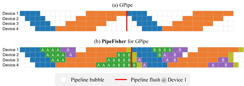
Figure 1: Schematic pipeline schedule (for two steps) of (a) GPipe Huang et al. (2019) and (b) PipeFisher for GPipe w/ 4 stages, 4 micro-batches, and 4 devices. Each colored box represents a work of forward (for a micro-batch), backward (for a micro-batch), curvature (for ${\bm{A}}_{l}$ or ${\bm{B}}_{l}$ of a micro-batch), inversion (for ${\bm{A}}_{l}$ or ${\bm{B}}_{l}$ of (a subset of) assigned layers), or precondition. PipeFisher utilizes the pipeline bubbles of multiple pipeline steps (two steps in this schedule) to refresh the curvature and inverse matrices once. Thus, precondition is the only computational overhead of PipeFisher over the standard pipeline schemes. The first precondition in this schedule is performed with the stale inverse matrices calculated at previous steps.

We note that unlike the other model partitioning approaches, the overhead of pipelining mainly comes from the low utilization of the accelerators rather than communication costs. To increase the utilization and throughput, efficient pipeline methods, e.g., GPipe Huang et al. (2019), 1F1B Narayanan et al. (2019), and Chimera Li & Hoefler (2021), have been proposed. It is possible to fill most bubbles with these methods when the number of micro-batches per accelerator is large enough. However, pipeline parallelism is often combined with data parallelism on massively parallel accelerators to achieve highest throughput Rajbhandari et al. (2021); Narayanan et al. (2021b). As a result, not enough micro-batches can be allocated to each accelerator to fill the bubbles efficiently.

In this work, we suggest to assign extra work (computation and communication) to the bubbles of pipelines to gain auxiliary benefits in LLM training in massively parallel settings. Auxiliary benefits in exchange for the extra work include avoidance of the catastrophic forgetting in learning through weight- or/and function-space regularizers Kirkpatrick et al. (2017); Pan et al. (2020), model compression based on weights and gradient magnitude Evci et al. (2020), and improved generalization performance by estimating the loss landscape Foret et al. (2021) and avoiding sharp minima Hochreiter & Schmidhuber (1997); Keskar et al. (2017). As an example in this direction whose benefits are relatively easy to observe and has reasonably complex work, we choose second-order optimization, which brings us the benefit of improved convergence and speeds up LLM training. And we propose PipeFisher, a training scheme that automatically assigns the work of K-FAC Martens & Grosse (2015), a second-order optimization method based on the Fisher information matrix, to the bubbles in any pipeline schedule. Figure 1 illustrates the pipeline schedule in our PipeFisher method for GPipe Huang et al. (2019). In Phase1 pretraining of BERT-Base and -Large, PipeFisher improves the GPU utilization in Chimera Li & Hoefler (2021), a state-of-the-art pipeline method, from 75.9% to 93.2% and from 59.8% to 97.6% and reduces the (simulated) training time to 48.7% and 75.7% compared to NVLAMB with Chimera, respectively.

2 Background and Related Work

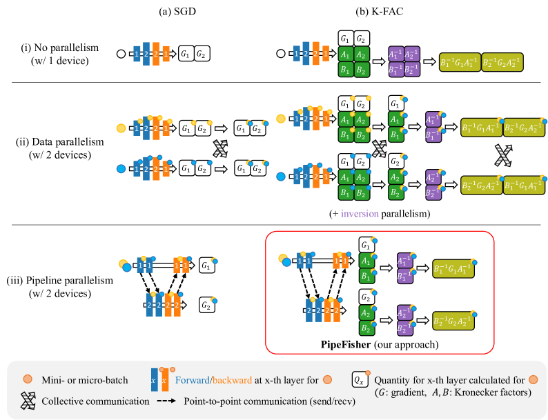
Figure 2: A gradient calculation (and preconditioning) step of (a) SGD and (b) K-FAC using (i) no parallelism, (ii) data parallelism (w/ 2 devices), and (iii) pipeline parallelism (w/ 2 stages, 1 layer/stage, 2 micro-batches, and 2 devices) for a two-layer neural network. In no-parallel and data-parallel K-FAC (i,b and ii,b), curvature (and collective communication after it) and inverse are usually performed once in many steps (e.g., 100 steps Pauloski et al. (2021)) to reduce the computational (and communication) overheads. Our pipeline-parallel K-FAC (PipeFisher) (iii,b) performs curvature and inverse in pipeline bubbles and refreshes the matrices once in a few steps (see Figure 1, Figure 3, and Figure 4). For every scheme of K-FAC, precondition is performed every step with fresh or stale inverse matrices (${\bm{A}}_{l}^{-1},{\bm{B}}_{l}^{-1}$) for fresh gradients (${\bm{G}}_{l}$).

In mini-batch-based training methods, the neural network model receives a mini-batch ${\mathcal{B}}=\{(x_{i},y_{i})\}$ of input example and target output, and the mini-batch loss is often evaluated as the average of per-example negative log likelihood of the target output given the input:

$${\mathcal{L}}_{\mathcal{B}}({\bm{\theta}}):=\frac{1}{|{\mathcal{B}}|}\sum_{i=1}^{|{\mathcal{B}}|}-\log p_{\bm{\theta}}(y_{i}|x_{i})=\left\langle-\log p_{\bm{\theta}}(y_{i}|x_{i})\right\rangle_{i\in{\mathcal{B}}}\,,$$

where ${\bm{\theta}}\in\mathbb{R}^{P}$ is a column vector of the model parameters, and $\left\langle\cdot\right\rangle_{i\in{\mathcal{B}}}$ represents the average over the mini-batch ${\mathcal{B}}$. The conditional probability $p_{\bm{\theta}}(y_{i}|x_{i})$ is calculated by performing a forward pass on the model followed by a softmax. The mini-batch gradient ${\bm{g}}:=\frac{\partial}{\partial{\bm{\theta}}}{\mathcal{L}}_{\mathcal{B}}({\bm{\theta}})\in\mathbb{R}^{P}$ is calculated by a backward pass and is used for the parameter update by gradient-based optimizers (e.g., SGD) (Figure 2(i,a)).

2.1 Distributed Parallel Deep Learning

Data parallelism: To increase the throughput (number of examples processed per unit time) of the forward and backward work, a mini-batch is sharded across multiple accelerators. Each accelerator has a copy of the identical model and performs forward and backward for a different shard of the mini-batch, i.e., micro-batch (or local mini-batch.) To keep model parameters common across the accelerators throughout the training, micro-batch gradients are synchronized through collective communication (i.e., allreduce) at every optimization step (Figure 2(ii,a)).

Pipeline parallelism: For a large model that does not fit the memory of an accelerator, the model is divided into multiple partitions or stages (sequences of the layers) and each accelerator performs forward and backward on the assigned stage in a pipeline. In synchronous pipeline methods, at the beginning and end of the pipeline (startup and tear-down), a stage needs to wait for the previous (or the next) stage’s forward (or backward) to complete, and there will be bubbles of time when some accelerators are idle. To better utilize the bubbles, it is a common approach to divide a mini-batch into multiple micro-batches Huang et al. (2019); Narayanan et al. (2019) and overlap the forward (or backward) work on different accelerators (Figure 2(iii,a)).

2.2 Natural Gradient Descent and Fisher Information Matrix

Natural gradient descent (NGD) Amari (1998) finds the steepest direction with respect to the Kullback-Leibler (KL) divergence between the model’s predictive distributions before and after the parameter update:

$$\mathrm{min}_{\Delta\in\mathbb{R}^{P}}{\mathcal{L}}_{\mathcal{B}}({\bm{\theta}}+\Delta)\mbox{ s.t. }KL(p_{\bm{\theta}}||p_{{\bm{\theta}}+\Delta})=const.$$

(cf. gradient descent finds the steepest direction with respect to the Euclidean distance between the parameters.) The constraint ensures that the model moves along the manifold of probability distributions at a constant rate Pascanu & Bengio (2014). Assuming $\Delta\rightarrow\bf{0}$, $KL(p_{\bm{\theta}}||p_{{\bm{\theta}}+\Delta})\approx\frac{1}{2}\Delta^{\top}{\bm{F}}\Delta$ (the second-order Taylor expansion), where ${\bm{F}}\in\mathbb{R}^{P\times P}$ is the Fisher information matrix (FIM):

$${\bm{F}}:=\mathbb{E}_{q}\left[\mathbb{E}_{p_{\bm{\theta}}}\left[\frac{\partial}{\partial{\bm{\theta}}}\log p_{\bm{\theta}}(y|x)\frac{\partial}{\partial{\bm{\theta}}}\log p_{\bm{\theta}}(y|x)^{\top}\right]\right]\,,$$ (1)

where $q$ is the input distribution, and we get the update direction $\Delta_{\rm NGD}\approx-{\bm{F}}^{-1}{\bm{g}}$. When the expectation $\mathbb{E}_{q}$ is replaced with the average over the minibatch ${\mathcal{B}}$, the FIM is equivalent to the generalized Gauss-Newton approximation Pearlmutter (1994) (positive semidefinite approximation) of the Hessian of the mini-batch loss ${\mathcal{L}}_{\mathcal{B}}$, and NGD can be seen as an approximate second-order optimization method Pascanu & Bengio (2014); Martens (2020). In practice of deep learning, the FIM is often estimated by the empirical Fisher Martens (2020):

$$\hat{{\bm{F}}}:=\left\langle\frac{\partial}{\partial{\bm{\theta}}}\log p_{\bm{\theta}}(y_{i}|x_{i})\frac{\partial}{\partial{\bm{\theta}}}\log p_{\bm{\theta}}(y_{i}|x_{i})^{\top}\right\rangle_{i\in{\mathcal{B}}}\,,$$

where both the expectation $\mathbb{E}_{q}$ and $\mathbb{E}_{p_{\bm{\theta}}}$ in Equation 1 are replaced with the average over the mini-batch ${\mathcal{B}}$. This allows the estimate of the FIM to be calculated during the backpropagation for the mini-batch loss ${\mathcal{L}}_{\mathcal{B}}$, leading to a faster training time Osawa et al. (2022).

Yet, the NGD is infeasible for deep neural network models with a large number of parameters ($P$ can be from millions to trillions Brown et al. (2020)) due to the huge computational and memory cost for constructing and inverting the (estimate of the) FIM (a $P\times P$ matrix).

2.3 Kronecker-Factored Approximate Curvature (K-FAC)

To make NGD practical, K-FAC Martens & Grosse (2015) approximates the curvature matrix in NGD (i.e., FIM) with an easy-to-invert matrix. Here we describe the K-FAC method for $L$-layer fully-connected neural network (ignoring the biases for simplicity). The (empirical) FIM is first approximated with a (1) layer-wise block-diagonal matrix (layer independence): $\hat{{\bm{F}}}\approx\mathrm{block\_diag}\left(\begin{array}[]{cccc}\hat{{\bm{F}}}_{1}&\hat{{\bm{F}}}_{2}&\cdots&\hat{{\bm{F}}}_{L}\end{array}\right)$ where $\hat{{\bm{F}}}_{l}\in\mathbb{R}^{P_{l}\times P_{l}}$ ($l=1,\dots,L$, $\sum_{l=1}^{L}P_{l}=P$) is the FIM for the parameters of the $l$-th layer. Then (2) the Kronecker factorization (input-output independence) is applied to each diagonal block:

$$\hat{{\bm{F}}}_{l} =\left\langle\frac{\partial}{\partial{\bm{\theta}}_{l}}\log p_{\bm{\theta}}(y_{i}|x_{i})\frac{\partial}{\partial{\bm{\theta}}_{l}}\log p_{\bm{\theta}}(y_{i}|x_{i})^{\top}\right\rangle_{i\in{\mathcal{B}}}$$

$$=\left\langle\left({\bm{a}}_{l}^{(i)}\otimes{\bm{e}}_{l}^{(i)}\right)\left({{\bm{a}}_{l}^{(i)}}\otimes{{\bm{e}}_{l}^{(i)}}\right)^{\top}\right\rangle_{i\in{\mathcal{B}}}$$

$$=\left\langle{\bm{a}}_{l}^{(i)}{{\bm{a}}_{l}^{(i)}}^{\top}\otimes{\bm{e}}_{l}^{(i)}{{\bm{e}}_{l}^{(i)}}^{\top}\right\rangle_{i\in{\mathcal{B}}}$$

$$\approx\underbrace{\left\langle{\bm{a}}_{l}^{(i)}{{\bm{a}}_{l}^{(i)}}^{\top}\right\rangle_{i\in{\mathcal{B}}}}_{=:{\bm{A}}_{l}\in\mathbb{R}^{d^{in}_{l}\times d^{in}_{l}}}\otimes\underbrace{\left\langle{\bm{e}}_{l}^{(i)}{{\bm{e}}_{l}^{(i)}}^{\top}\right\rangle_{i\in{\mathcal{B}}}}_{=:{\bm{B}}_{l}\in\mathbb{R}^{d^{out}_{l}\times d^{out}_{l}}}\in\mathbb{R}^{P_{l}\times P_{l}}\,.$$

${\bm{a}}_{l}^{(i)}\in\mathbb{R}^{d^{in}_{l}\times 1}$ is the input to the $l$-th layer (activations from the previous layer) for the $i$-th example, ${\bm{e}}_{l}^{(i)}\in\mathbb{R}^{d^{out}_{l}\times 1}$ is the gradient of ${\mathcal{L}}_{\mathcal{B}}$ with respect to the outputs (errors) of the $l$-th layer for the $i$-th example, and ${\bm{\theta}}_{l}\in\mathbb{R}^{P_{l}}$ ($P_{l}=d^{in}_{l}\cdot d^{out}_{l}$) is the set of parameters of the $l$-th layer ($l=1,\dots,L$). $\otimes$ represents the Kronecker product of two matrices (or vectors): for ${\bm{A}}\in\mathbb{R}^{d_{1}\times d_{2}}$ and ${\bm{B}}\in\mathbb{R}^{d_{3}\times d_{4}}$,

$${\bm{A}}\otimes{\bm{B}}:=\left[\begin{array}[]{ccc}A_{1,1}{\bm{B}}&\cdots&A_{1,d_{2}}{\bm{B}}\\ \vdots&\ddots&\vdots\\ A_{d_{1},1}{\bm{B}}&\cdots&A_{d_{1},d_{2}}{\bm{B}}\end{array}\right]\in\mathbb{R}^{d_{1}d_{3}\times d_{2}d_{4}}\,.$$

2.3.1 Work in K-FAC

Besides the forward and backward computations for calculating gradients, K-FAC requires additional work per optimization step (Figure 2(i,b)).

Curvature work: The Kronecker factors ${\bm{A}}_{l}\in\mathbb{R}^{d^{in}_{l}\times d^{in}_{l}}$ and ${\bm{B}}_{l}\in\mathbb{R}^{d^{out}_{l}\times d^{out}_{l}}$ ($l=1,\dots,L$) can be calculated by concatenating per-example activations and errors and performing matrix-matrix multiplications:

$${\bm{U}}_{A,l} :=\frac{1}{\sqrt{|{\mathcal{B}}|}}\left[\begin{array}[]{ccc}{\bm{a}}_{l}^{(1)}&\cdots&{\bm{a}}_{l}^{(|{\mathcal{B}}|)}\end{array}\right]\in\mathbb{R}^{d^{in}_{l}\times|{\mathcal{B}}|}\,,$$

$${\bm{U}}_{B,l} :=\frac{1}{\sqrt{|{\mathcal{B}}|}}\left[\begin{array}[]{ccc}{\bm{e}}_{l}^{(1)}&\cdots&{\bm{e}}_{l}^{(|{\mathcal{B}}|)}\end{array}\right]\in\mathbb{R}^{d^{out}_{l}\times|{\mathcal{B}}|}\,,$$

$${\bm{A}}_{l} ={\bm{U}}_{A,l}{\bm{U}}_{A,l}^{\top}\,,\mbox{ and }{\bm{B}}_{l}={\bm{U}}_{B,l}{\bm{U}}_{B,l}^{\top}\,.$$

In PyTorch Paszke et al. (2019), this can be implemented by calling torch.matmul() for each of ${\bm{A}}_{l}$ and ${\bm{B}}_{l}$ for every layer ($2\times L$ calls in total).

Inversion and precondition work: After constructing the Kronecker factors ${\bm{A}}_{l}$ and ${\bm{B}}_{l}$, we can get the approximate layer-wise natural gradient as follows:

$$\hat{{\bm{F}}}_{l}^{-1}{\bm{g}}_{l}\approx\left({\bm{A}}_{l}\otimes{\bm{B}}_{l}\right)^{-1}{\bm{g}}_{l} =\left({\bm{A}}_{l}^{-1}\otimes{\bm{B}}_{l}^{-1}\right){\bm{g}}_{l}$$

$$=\mathrm{vec}\left({\bm{B}}_{l}^{-1}{\bm{G}}_{l}{\bm{A}}_{l}^{-1}\right)\in\mathbb{R}^{P_{l}}\,,$$

where ${\bm{g}}_{l}\in\mathbb{R}^{P_{l}}$ is the gradient of the loss with respect to the parameters of the $l$-th layer ($l=1,\dots,L$, ${\bm{g}}=\left[\begin{array}[]{ccc}{\bm{g}}_{1}^{\top}&\cdots&{\bm{g}}_{L}^{\top}\end{array}\right]^{\top}$). Here we exploit two properties of a Kronecker product: $\left({\bm{A}}\otimes{\bm{B}}\right)^{-1}={\bm{A}}^{-1}\otimes{\bm{B}}^{-1}$ and $({\bm{A}}\otimes{\bm{B}})\mathrm{vec}\left({\bm{X}}\right)=\mathrm{vec}\left({\bm{B}}{\bm{X}}{\bm{A}}\right)$. $\mathrm{vec}(\cdot)$ is an operator that vectorizes a matrix by stacking its columns, and ${\bm{g}}_{l}=\mathrm{vec}({\bm{G}}_{l})$. This reduces the computational complexity for the inversion from ${\mathcal{O}}(P_{l}^{3})$ to ${\mathcal{O}}({d^{in}_{l}}^{3}+{d^{out}_{l}}^{3})$. Also, we can avoid the memory consumption for materializing the Kronecker product ${\bm{A}}_{l}\otimes{\bm{B}}_{l}$ and its inverse. As each Kronecker factor is a symmetric matrix, we can calculate its inverse by utilizing Cholesky decomposition. In PyTorch, we call torch.linalg.cholesky() followed by torch.linalg.cholesky_inverse() for every Kronecker factor ($2\times L$ calls in total). Finally, we call torch.matmul two times ($2\times L$ calls in total) to get the preconditioned gradient ${\bm{B}}_{l}^{-1}{\bm{G}}_{l}{\bm{A}}_{l}^{-1}$ ($l=1,\dots,L$).

In practice, curvature and inversion work are performed only once in many optimization steps, depending on the model size, data size, and available computing resource (e.g., 10 steps for curvature and 100 steps for inversion for pretraining BERT-Large in Pauloski et al. (2021)) to reduce the computational overheads of K-FAC. In this case, precondition of the gradients of the current optimization step will be performed using the stale inverse matrices that are calculated at the previous steps.

2.3.2 Distributed Parallel K-FAC Schemes

CPU offloading: Ba et al. (2017) proposed a distributed parallel K-FAC scheme that has multiple gradient workers for forward and backward work (data parallelism), a stats worker for curvature and inversion work, and a parameter server for preconditioning and updating the parameters. The stats worker asynchronously calculates ${\bm{A}}_{l},{\bm{B}}_{l},{\bm{A}}_{l}^{-1},$ and ${\bm{B}}_{l}^{-1}$ ($l=1,\dots,L$) for a mini-batch on a CPU while the gradient workers process multiple mini-batches on accelerators (GPUs). Once the inverse matrices are ready, they are sent to the parameter server and are used for preconditioning. Anil et al. (2021) also adopt CPU offloading of curvature and inversion work for a distributed version of Shampoo optimizer Gupta et al. (2018) which requires to construct and invert the Kronecker-factored AdaGrad Duchi et al. (2011) matrix (i.e., second moment matrix of mini-batch gradients) of the same shapes as the Kronecker-factored FIM in K-FAC. Because constructing and inverting matrices on CPUs can be much slower than a forward and a backward work on accelerators, the inverse matrices used for preconditioning can be stale for many steps (e.g., 100-1000 steps). In this scheme, the frequency of refreshing the inverse matrices is bounded by the CPU performance compared to the accelerators.

Data and inversion parallelism: Osawa et al. (2019) proposed a hybrid scheme of data parallelism and inversion parallelism where each accelerator performs forward, backward, and curvature work for a different micro-batch (data parallelism) and performs inversion and preconditioning work for different layers (inversion parallelism) (illustrated in Figure 2(ii,b)). This approach efficiently reduces the per-step computational and memory costs of K-FAC, which mainly come from the inversion work, and scales to as many distributed accelerators as the number of layers in the model. Yet, the curvature work for all the layers need to be performed by each accelerator. Moreover, this scheme introduces an additional work, i.e., the communication of dense matrices (Kronecker factors of each layer) among distributed accelerators due to the data parallelism, and this will be the main bottleneck in massively parallel settings Ueno et al. (2020). To mitigate these computational and communication costs per step, it is a common strategy to apply a manually selected frequency (e.g., once in 100 steps) for refreshing the inverse matrices Pauloski et al. (2020; 2021).

3 PipeFisher

We propose PipeFisher, a training scheme that assigns the K-FAC work, i.e., curvature, inverse, and precondition, to bubbles in pipelines (Figure 1 and Figure 2(iii,b)). PipeFisher has several advantage over the CPU-offloading and data- and inversion-parallel K-FAC (Figure 2(ii,b)): (i) each accelerator only needs to store the parameters, gradients, and curvature matrices for the layers in the assigned pipeline stage, resulting in smaller memory consumption; (ii) the inverse work are split among multiple accelerators without collective communication; (iii) because PipeFisher leverages bubbles to perform curvature and inverse work, these computations do not affect training throughput; and (iv) since these computations are performed on accelerators, which is much faster than on CPUs, the matrices can be refreshed much more frequently (e.g., once in 2-3 steps). This is expected to allow for more stable convergence and more aggressive learning rates since it is observed that the value of curvature matrix fluctuates greatly, especially in the early phase of the training Osawa et al. (2019).

3.1 Automatic Work Assignments

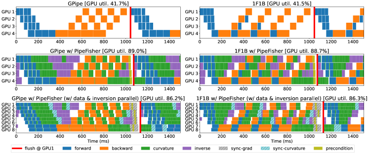
Figure 3: Profiled CUDA kernel execution times on NVIDIA P100 GPUs for 5th and (part of) 6th pipeline steps in GPipe (left) and 1F1B (right) w/ Adam (top) and w/ PipeFisher w/o (middle) and w/ (bottom) data and inversion parallelism in pretraining BERT-Base ($L=12$) w/ 4 stages (3 layers/stage), 4 or 8 GPUs, 4 micro-batches of size 32 per GPU per step, and sequence length 128.

Our goal is to refresh the curvature and inverse matrices as frequently as possible by utilizing the bubbles (idle accelerators) in any pipeline schedule (e.g., GPipe, 1F1B, Chimera) as much as possible. To this end, PipeFisher automatically assigns K-FAC work to bubbles using several rules:

1. A curvature work for ${\bm{A}}_{l}$ or ${\bm{B}}_{l}$ (for a micro-batch and for a layer) is assigned to a bubble after forward or backward (for the corresponding micro-batch and layer), respectively.

2. An inversion work for ${\bm{A}}_{l}$ or ${\bm{B}}_{l}$ (for a layer) is assigned to a bubble after the curvature work for ${\bm{A}}_{l}$ or ${\bm{B}}_{l}$ for all the micro-batches (for the corresponding layer), respectively.

3. Precondition work are assigned after backward for all the layers in a stage and before the beginning of the next pipeline step.

We first collect the profile of the CUDA kernel execution times of the standard work (i.e., forward and backward) during a step of a pipeline schedule followed by K-FAC work (i.e., curvature, inversion, and precondition) on GPUs. Then we pick one work from the ‘queue’ of all the K-FAC work and assign it to a bubble if its duration is shorter than the bubble duration (otherwise, subsequent bubbles are utilized) according to the rules above. We repeat this procedure until all the K-FAC work are assigned to bubbles. Once all the K-FAC work are assigned (and the queue becomes empty), we finalize the (static) schedule and use it repeatedly until the training is completed. Curvature and inversion work often take a few steps (e.g., 2-3 steps) to complete (cf.$\sim$100-1000 steps in previous works), whereas precondition is performed every step. If the inverse matrix of a layer is not ready, the one previously calculated for that layer is used for precondition.

Figure 3 shows the profiling results (using NVIDIA’s Nsight) of GPipe and 1F1B pipeline steps w/o and w/ automatically assigned K-FAC work. Comparing the top and middle figures for GPipe and 1F1B, it can be seen that PipeFisher is making good use of the bubbles (GPU utilization is increased from about 42% to 89%), with precondition work being the only major computational overhead. In this setup, the curvature and inverse matrices are refreshed within a maximum of 2 steps (1 step for the second and third stages and 2 steps for the other stages).

3.2 Combination with data and inversion parallelism

PipeFisher (and the automatic work assignments) can be combined with data and inversion parallelism. The bottom figures in Figure 3 show the profiled timeline with the number of GPUs doubled (from 4 GPUs to 8 GPUs, 2 GPUs per stage.) For the data parallelism, collective communication (sync-grad and sync-curvature) is performed between GPUs responsible for the same pipeline stage (e.g., GPU1 and GPU2 for stage1) to synchronize gradient and curvature. Since the inversion work (for 3 layers per stage) are split among 2 GPUs, the communication cost for curvature synchronization is amortized. Thus, only gradient synchronization (as with distributed SGD and distributed Adam) is the main communication overhead.

Figure 4: Profiled CUDA kernel execution times on NVIDIA P100 GPUs for 5-7th pipeline steps in Chimera Li & Hoefler (2021) w/ Adam (top) and w/ PipeFisher w/ data and inversion parallelism (bottom) in pretraining BERT-Large ($L=24$, ) w/ 8 stages (3 layers/stage), 8 GPUs, 8 micro-batches of size 32 per GPU per step, and sequence length 128.

To better demonstrate the effectiveness of the automatic work assignments, we target the Chimera Li & Hoefler (2021) pipeline schedule which is even more complex and more efficient than GPipe and 1F1B. Chimera handles multiple pipelines simultaneously to make effective use of bubbles and efficiently increase throughput. Figure 4 (top) shows the pipeline schedule in Chimera using two bidirectional pipelines (up pipeline and down pipeline). Since each GPU is responsible for two stages simultaneously, gradient synchronization (sync-grad) is performed for data parallelism between GPUs responsible for the same stage (e.g., GPU 1 and 8 for stage 1 and 8, GPU 4 and 5 for stage 4 and 5.) Figure 4 (bottom) shows the results of applying PipeFisher (with data and inversion parallelism) to Chimera; PipeFisher increases GPU utilization from 59.8% to 97.6%. With this setup, curvature and inverse matrices are refreshed in 4 steps for stages 1 and 8, and in 2 steps for the other stages.

3.3 Performance Modeling

The number of pipeline steps required to complete the curvature and inversion work determines how often the curvature information is refreshed. Also, these work require additional memory consumption, which can limit the model size and micro-batch size. To estimate the frequency of matrix updates and the total memory consumption, we create a performance model. Table 1 lists frequently used symbols.

Table 1: Symbols

$D$	The number of pipeline stages (depth)
$N_{micro}$	The number of micro-batches per device within a training iteration
$B_{micro}$	Micro-batch size
$B_{mini}$	Mini-batch size ($=B_{micro}*N_{micro}*W$)
$M_{\theta}$	Memory consumption for the parameters of one stage
$M_{act}$	Memory consumption for the activations of one stage for one micro-batch
$M_{err}^{peak}$	Peak memory consumption for the errors of one stage for one micro-batch
$C_{{\color[rgb]{0.12109375,0.46484375,0.70703125}f}}$, $C_{{\color[rgb]{1,0.49609375,0.0546875}b}}$	The number of forward, backward passes on the critical path in a pipeline step (when $N_{micro}=D$, $C_{{\color[rgb]{0.12109375,0.46484375,0.70703125}f}}=C_{{\color[rgb]{1,0.49609375,0.0546875}b}}=2D-1$ for GPipe and 1F1B (w/ pipeline flush) and $C_{{\color[rgb]{0.12109375,0.46484375,0.70703125}f}}=D$, $C_{{\color[rgb]{1,0.49609375,0.0546875}b}}=2D-2$ for Chimera)

(a) Modeled time per step and memory consumption

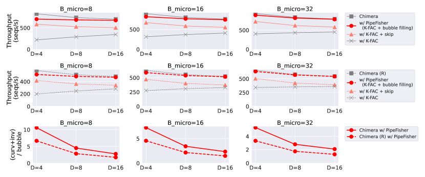
(b) Modeled throughput (sequences/s) and (curvature+inversion)-bubble ratio

Figure 5: Performance model for Chimera (w/ 2 pipelines) with $D$ BERT-Base blocks (one block per pipeline stage) with $N_{micro}=D$ on an NVIDIA P100. “w/ PipeFisher (K-FAC + bubble filling)”: The pipeline bubbles are filled with the curvature and inversion work of K-FAC, and only the precondition work is the computational overhead of PipeFisher over the vanilla Chimera. “w/ K-FAC + skip”: Naive K-FAC execution (i.e., every K-FAC work is performed without utilizing the bubbles) with the curvature and inversion work skipped every (curv+inv)/bubble iterations, i.e., the same frequency as PipeFisher. “w/ K-FAC”: Naive K-FAC execution without skipping. R indicates activation recomputation.

For simplicity, P2P communication costs are ignored in the modeling since there are few gaps (i.e., latency for P2P communication) between forwards and backwards in the profile results in Figure 3 and Figure 4. We also ignore the cost of collective communication (i.e., sync-grad and sync-curvature) since our goal here is to model the duration of the bubbles and the size of the K-FAC work. Assuming that all pipeline stages have the same size model partition, we put $T_{{\color[rgb]{0.12109375,0.46484375,0.70703125}f}}$ and $T_{{\color[rgb]{1,0.49609375,0.0546875}b}}$ as the computation time of forward and backward for one micro-batch, respectively. Then one pipeline step time $T_{pipe}=C_{{\color[rgb]{0.12109375,0.46484375,0.70703125}f}}T_{{\color[rgb]{0.12109375,0.46484375,0.70703125}f}}+C_{{\color[rgb]{1,0.49609375,0.0546875}b}}T_{{\color[rgb]{1,0.49609375,0.0546875}b}}$ and the total bubble time $T_{bubble}=T_{pipe}-N_{micro}(T_{{\color[rgb]{0.12109375,0.46484375,0.70703125}f}}+T_{{\color[rgb]{1,0.49609375,0.0546875}b}})$. The worst case memory consumption (among all pipeline stages) is modeled as: $M_{pipe}=2\frac{DW}{\#devices}M_{\theta}+N_{micro}M_{act}+M_{err}^{peak}$. The time and memory overheads for the K-FAC work are:

$$T_{kfac}^{+} =\underbrace{N_{micro}T_{{\color[rgb]{0.171875,0.62890625,0.171875}curv}}+T_{{\color[rgb]{0.58203125,0.40234375,0.7421875}inv}}}_{\mbox{fit into bubbles}}+T_{{\color[rgb]{0.73828125,0.7421875,0.1328125}prec}}$$

$$\mbox{and\,\,\,}M_{kfac}^{+} =M_{{\color[rgb]{0.171875,0.62890625,0.171875}curv}}+M_{{\color[rgb]{0.58203125,0.40234375,0.7421875}inv}}+N_{micro}M_{err}^{save}\,,$$

where $T_{{\color[rgb]{0.171875,0.62890625,0.171875}curv}}/M_{{\color[rgb]{0.171875,0.62890625,0.171875}curv}}$, $T_{{\color[rgb]{0.58203125,0.40234375,0.7421875}inv}}/M_{{\color[rgb]{0.58203125,0.40234375,0.7421875}inv}}$, and $T_{{\color[rgb]{0.73828125,0.7421875,0.1328125}prec}}$ represent the time/memory for curvature (for one micro-batch), inversion, and precondition work for one stage, respectively ($M_{{\color[rgb]{0.171875,0.62890625,0.171875}curv}}=M_{{\color[rgb]{0.58203125,0.40234375,0.7421875}inv}}$.) And $M_{err}^{save}$ is the memory cost to keep the errors ${\bm{e}}_{l}$ for calculating the Kronecker factors ${\bm{B}}_{l}$ (for one micro-batch) (the memory cost to keep the activations ${\bm{a}}_{l}$ for ${\bm{A}}_{l}$ is included in $M_{pipe}$.) We take microbenchmarks and measure the times and memories for different $B_{micro}$, $D$, pipeline methods (GPipe, 1F1B, or Chimera) and BERT models (Base or Large) on an NVIDIA P100 GPU.

Figure 5 shows the performance model for a pipeline stage of Chimera with a BERT-Base layer (assuming the BERT-Base model has $D$ layers in total). Doubling the number of layers per pipeline stage doubles all times and memories. Here we set $N_{micro}=D$, in which case the time, memory, and bubble ratio are the same in GPipe and 1F1B.

Computation time and throughput: The top row of Figure 5 (a) shows the breakdown of computation time per step. There are five bars for each $(B_{micro},D)$ combination, showing $T_{pipe}+T_{{\color[rgb]{0.73828125,0.7421875,0.1328125}prec}}$, $T_{bubble}$, $T_{pipe}+T_{{\color[rgb]{0.73828125,0.7421875,0.1328125}prec}}$ with activation recomputation (R), $T_{bubble}$ with activation recomputation (R), and $T_{kfac}^{+}-T_{{\color[rgb]{0.73828125,0.7421875,0.1328125}prec}}$, where R indicates the activation recomputation Griewank & Walther (2000) for saving memory consumption. $T_{pipe}+T_{{\color[rgb]{0.73828125,0.7421875,0.1328125}prec}}$ corresponds to the computation time per step of PipeFisher. Because $T_{{\color[rgb]{0.73828125,0.7421875,0.1328125}prec}}$ is relatively small, the computational overhead of PipeFisher compared to the vanilla pipeline is small. The top and middle rows of Figure 5 (b) compare the throughput of the vanilla pipeline and PipeFisher and show little difference between them. As $B_{micro}$ and $D$ $(=N_{micro})$ increase, $T_{pipe}$, $T_{bubble}$, and $N_{micro}T_{{\color[rgb]{0.171875,0.62890625,0.171875}curv}}$ increase, while $T_{{\color[rgb]{0.58203125,0.40234375,0.7421875}inv}}$ is constant regardless of $B_{micro}$ or $D$, so that $N_{micro}T_{{\color[rgb]{0.171875,0.62890625,0.171875}curv}}+T_{{\color[rgb]{0.58203125,0.40234375,0.7421875}inv}}<2\cdot T_{bubble}$ when $B_{micro}$ and $D$ is relatively large, and curvature and inversion work can be hidden within pipeline bubble in two pipeline iterations. The bottom row of Figure 5 (b) shows the ratio of $N_{micro}T_{{\color[rgb]{0.171875,0.62890625,0.171875}curv}}+T_{{\color[rgb]{0.58203125,0.40234375,0.7421875}inv}}$ to $T_{bubble}$, suggesting the number of pipeline steps required for PipeFisher to refresh the curvature information. Through the effective use of bubbles, PipeFisher updates curvature information at a high frequency with a high throughput that cannot be achieved by simply skipping updates without utilizing the bubbles (“w/ PipeFisher” vs. “w/ K-FAC + skip” in Figure 5 (b)).

Memory consumption: The bottom row of Figure 5 (a) shows the breakdown of memory consumption. There are two bars for each $(B_{micro},D)$ combination, showing $N_{micro}M_{act}+M_{err}^{peak}+M_{\theta}+M_{kfac}^{+}$ without/with R. $N_{micro}M_{act}$ and $N_{micro}M_{err}^{save}$ account for most of the memory consumption when $B_{micro}$ or $D$ $(=N_{micro})$ is large, while $M_{{\color[rgb]{0.171875,0.62890625,0.171875}curv}}$ $(=M_{{\color[rgb]{0.58203125,0.40234375,0.7421875}inv}})$ is constant. Activation recomputation (R) reduces throughput (due to the additional forward work) and increases $T_{bubble}$, but at the same time significantly reduces memory consumption by $M_{act}$. In this case, $N_{micro}M_{err}^{save}$, $M_{{\color[rgb]{0.171875,0.62890625,0.171875}curv}}$, and $M_{{\color[rgb]{0.58203125,0.40234375,0.7421875}inv}}$, i.e., $M_{kfac}^{+}$, are the major bottlenecks. As $T_{bubble}$ is increased by activation recomputation, curvature information is updated at a higher frequency.

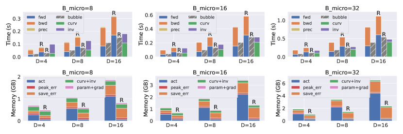
(a) Modeled time per step and memory consumption of GPipe and 1F1B (w/ pipeline flush)

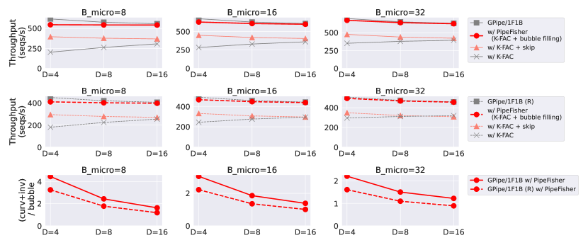
(b) Modeled throughput (sequences/s) and (curvature+inversion)-bubble ratio of GPipe and 1F1B (w/ pipeline flush)

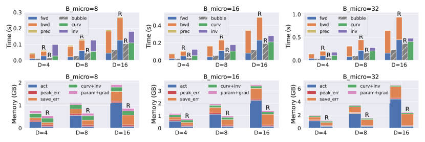
(c) Modeled time per step and memory consumption of Chimera w/ $2$ pipelines

(d) Modeled throughput (sequences/s) and (curvature+inversion)-bubble ratio of Chimera w/ $2$ pipelines

Figure 9: Performance model for $D$ BERT-Base blocks (one block per pipeline stage) with $N_{micro}=D$ on an NVIDIA P100. R indicates activation recomputation.

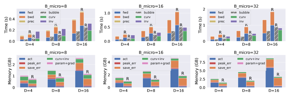
(a) Modeled time per step and memory consumption of GPipe and 1F1B (w/ pipeline flush)

(b) Modeled throughput (sequences/s) and (curvature+inversion)-bubble ratio of GPipe and 1F1B (w/ pipeline flush)

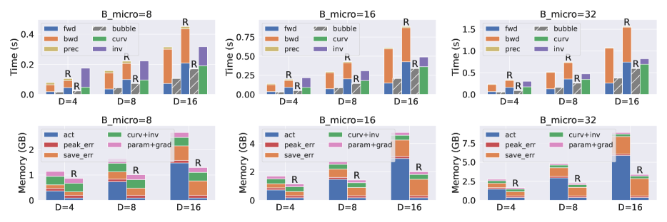
(c) Modeled time per step and memory consumption of Chimera w/ $2$ pipelines

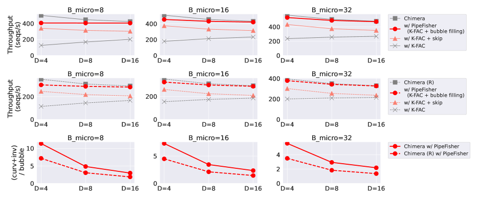
(d) Modeled throughput (sequences/s) and (curvature+inversion)-bubble ratio of Chimera w/ $2$ pipelines

Figure 10: Performance model for $D$ BERT-Large blocks (one block per pipeline stage) with $N_{micro}=D$ on an NVIDIA P100. R indicates activation recomputation.

Figure 9 and Figure 10 in Appendix A summarize the performance models for BERT-Base and BERT-Large, respectively, with GPipe/1F1B or Chimera. Chimera consistently achieves higher throughput than GPipe and 1F1B (due to the smaller $T_{bubble}$), but instead the curvature information is updated less frequently. Therefore, the pipeline method can be selected based on the tradeoff between throughput and the frequency of extra information (i.e., curvature information for K-FAC) updates.

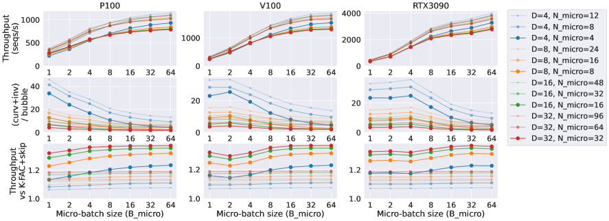
Figure 6: Modeled throughput (sequences/s) and (curvature+inversion)-bubble ratio of Chimera w/ $2$ pipelines w/ PipeFisher for $D$ BERT-Base blocks ($D\in\{4,8,16,32\}$, one block per pipeline stage) on an NVIDIA P100, V100, and RTX3090. “Throughput vs K-FAC+skip”: Ratio of the throughput of PipeFisher to a naive K-FAC execution (i.e., every K-FAC work is performed without utilizing the bubbles) with the curvature and inversion work skipped every (curv+inv)/bubble iterations, i.e., the same frequency as PipeFisher.

To better understand the scaling behavior of PipeFisher, we make the same observations (i.e., throughput and (curvature+inversion)-bubble ratio) with various Transformer architectures (w/ different sequence lengths $S$), mini-/micro-batch sizes ($B_{mini}=N_{micro}\cdot B_{micro}$), and hardware (NVIDIA P100, V100, and RTX3090). This time we will focus only on Chimera, which has fewer bubbles and achieves a higher throughput than GPipe and 1F1B. Figure 6 shows the results for BERT-Base. Other results are listed in Table 3. Below is a summary of observations:

• Since the precondition work (independent of $B_{mini}=N_{micro}\cdot B_{micro}$) is relatively small in all settings, little difference in throughput is observed between Chimera and Chimera w/ PipeFisher. Therefore, only the throughput of Chimera w/ PipeFisher is shown.

• As the micro-batch size $B_{micro}$ is increased, the (curvature+inversion)-bubble ratio becomes smaller (i.e., easier to fit extra work to the bubbles) because the cost of the inversion work is relatively small.

• Furthermore, as the pipeline depth $D$ increases, the ratio goes down because the bubble increases.

• On the other hand, as the number of micro-batches $N_{micro}$ is increased, the ratio increases because the bubbles become smaller.

• Transformers with longer sequence lengths $S$ have larger bubbles and smaller ratios. This is because the total number of tokens ($S\cdot N_{micro}\cdot B_{micro}$) linearly increases the forward, backward, and curvature work, while inversion work is independent of it.

• The change in the ratio in different hardware depends on the Transformer architecture (i.e., a faster GPU increases, decreases, or does not change the ratio).

• In most cases the ratio is in the range of 2-10, except when the micro-batch size $B_{micro}$ is particularly small (e.g., 1,2) and the number of micro-batches $N_{micro}$ is large (e.g., $N_{micro}=3D$). This suggests that curvature information is updated at a high frequency.

• PipeFisher provides up to about $1.4\times$ speedup versus naive K-FAC execution with curvature-/inversion-skipping (“K-FAC+skip”) when $N_{micro}=D$ and $B_{micro}$ is large (64). On the other hand, when the number of micro-batches is large (e.g., $N_{micro}=3D$) or $B_{micro}$ is small, speedup by PipeFisher is limited to about $1.1\times$.

4 Language Modeling

We apply PipeFisher to the pretraining of BERT-Base and -Large models Devlin et al. (2019) on the English Wikipedia Wikipedia (see Appendix for information on preparing the dataset.) The task is to minimize the sum of the masked language modeling loss (classification with vocabulary size 30,522) and next sentence prediction loss (binary classification). BERT pretraining consists of two phases, where the maximum sequence lengths are 128 and 512, respectively. The learning rate, mini-batch size and number of steps for each phase depends on the implementation, but the number of steps in Phase 1 often accounts for 80-90% of the total (90% in the original work Devlin et al. (2019)). We use NVLAMB, NVIDIA’s implementation of the LAMB optimizer You et al. (2020), as the baseline optimizer to be compared with K-FAC (with PipeFisher). As the full pretraining of BERT requires a huge amount of energy and CO₂ overheads, we only discuss the training time in Phase 1. Following Pauloski et al. (2022) Pauloski et al. (2022), we apply K-FAC to all fully-connected layers except for the final classification head, where $d^{out}_{L}=30,522$ (vocabulary size) and the Kronecker factor ${\bm{B}}_{L}$ will be too large to construct/invert, and we use NVLAMB for the rest of layers. Hereafter, for simplicity, we refer to this as K-FAC.

Figure 7: Left: Pretraining BERT-Base on the English Wikipedia (Phase 1: mini-batch size 8K, sequence length 128 for 7,038 steps) using NVLAMB and K-FAC. Right: Same training curves as on the left applying time per step measured on 256 P100 GPUs using Chimera for NVLAMB (GPU util.: 75.9%) and Chimera with PipeFisher for K-FAC (GPU util.: 93.2%) (with 4 pipeline stages). With this setup, PipeFisher updates the inverse every 5 to 10 steps. Each curve is smoothed by applying signal filters using SciPy v1.8.0 (y_smooth = signal.filtfilt(*signal.butter(3, 0.05), y)). The number of steps and time for K-FAC to reach NVLAMB’s final loss (3.41) are calculated for the smooth curves (ignoring large fluctuations around the 1,000th step.)

BERT-Base: We first train BERT-Base using NVLAMB and K-FAC. Our training code is based on NVIDIA’s PyTorch-based codebase for BERT pretraining and we use the same training hyperparamers for NVLAMB — mini-batch size 8,192, weight decay 0.01, base learning rate $6\cdot 10^{-3}$, training steps 7,038, and linear learning rate warming up steps 2,000. For K-FAC, the same hyperparameters are used except that the number of learning rate warming up steps is reduced to 600, resulting in larger learning rates than NVLAMB until the 2,000th step (see Appendix for more information on training settings.) We observed that during the first 1,000-2,000 steps, K-FAC benefits from a more aggressive learning rate, whereas training diverges when the same learning rate is applied to NVLAMB. Figure 7 shows the pretraining loss versus the number of steps and training time. K-FAC significantly improves the convergence and reaches NVLAMB’s final loss (3.41) in 2,961 steps (42.0% of 7038 steps). For measuring the wall-clock time, we run NVLAMB by Chimera and K-FAC by Chimera with PipeFisher on 256 GPUs with 4 pipeline stages (thus 64 model copies) and 4 micro-batches of size 32 per optimization step ($4\times 32\times 64=8,192$.) As the precondition work is the only major computational overhead, PipeFisher retains the improved convergence by K-FAC and reaches NVLAMB’s final loss in 48.4 minutes (48.7% of 99.4 minutes) while improving the GPU utilization from 75.9% to 93.2%.

BERT-Large: Next, we target BERT-Large model. Since pretraining BERT-Large is resource-intensive, we rely on the results of Pauloski et al. (2022) Pauloski et al. (2022) for the number of training steps by NVLAMB and (data- and inversion-parallel) K-FAC (with inverse refreshed once every 50 steps) and the SQuAD v1.1 F1 score after fine tuning. In addition to this, their Phase 1 results use a mini-batch of size 64K, so setting the micro-batch size to 32 (maximum number of powers of 2 that can be placed on a P100 GPU) would require a 2K GPUs, which requires a huge computing budget. So, we instead apply the time per step with Chimera w/ and w/o PipeFisher measured on 8 GPUs as in Figure 4 to simulate the training time, i.e., ignoring the increase in communication costs when scaling from 8 GPUs to 2K GPUs. The results are summarized in Table 2. As the computational overhead per step with PipeFisher is only $\sim$6.5%, the Phase 1 training time is reduced from 275.1 to 208.3 minutes (75.7%) (in the simulation) by improving the GPU utilization from 59.8% to 97.6% and taking advantage of the convergence improved by K-FAC.

Table 2: Pretraining BERT-Large on the English Wikipedia (Phase 1: mini-batch size 64K, Phase 2: mini-batch size 32K) using NVLAMB and K-FAC. We use the results from Pauloski et al. (2022) for the number of steps in Phase 1 and Phase 2 and the SQuAD v1.1 F1 score after fine tuning. * We apply time per step measured on 8 P100 GPUs using Chimera for NVLAMB (GPU util.: 59.8%) and Chimera with PipeFisher for K-FAC (GPU util.: 97.6%) (same setting as Figure 4) to simulate the training time.

Optimizer	Pipeline scheme	Phase 1			Phase 2	F1
		Steps	Time/step∗	Time∗	Steps
NVLAMB	Chimera	7038	2345.6 ms	275.1 min	1563	90.1%
K-FAC	Chimera w/ PipeFisher	5000	2499.5 ms	208.3 min	1563	90.15%

5 Discussion and Conclusion

PipeFisher for non-Transformer architectures: PipeFisher is applicable to any neural architecture that can be pipelined. As a Transformer model is composed of multiple encoder/decoder layers of the same size (except for embedding layers and task-specific heads), it is easy to distribute the work equally among pipeline stages, making it a particularly good match for pipelining and PipeFisher. On the other hand, other architectures, such as convolutional neural networks, often have different numbers of neurons/channels and feature map sizes at each layer, so it is more challenging to apply pipelining and divide the work evenly. In particular, the computational cost of inversion work is proportional to the cube of the matrix size, which can easily cause load imbalance.

Extra work for other types of algorithms: The application of the idea of “assigning extra work to bubbles in pipeline for auxiliary benefits” is not limited to K-FAC. For example, pipelining the work of Shampoo optimizer Gupta et al. (2018), which also accelerates training Transformers Anil et al. (2021) and requires Kronecker-factored matrices of the same size as the K-FAC (for fully-connected layers), is a natural extension of the PipeFisher. Since the Shampoo optimizer requires an eigenvalue decomposition, which is computationally more expensive than an inversion, for each matrix, a method that divides the work for a single matrix into multiple pieces would be necessary for an efficient bubble utilization. Another example, other than training acceleration, is the improvement of generalization performance through Sharpness-Aware Minimization (SAM) Foret et al. (2021). SAM requires an additional forward and backward for every training step to estimate the loss sharpness Hochreiter & Schmidhuber (1997); Keskar et al. (2017), so it contains twice the work of regular SGD and has the potential to double the accelerator utilization.

Limitations: To avoid the enormous energy and CO₂ overheads of pretraining LLMs, we do not conduct end-to-end time measurements. Instead, we simulate the time by multiplying the measured time per step by the total number of steps. For this reason, although the ability to update curvature information frequently is one advantage of PipeFisher over existing distributed K-FAC approaches (see the first paragraph of Section 3), this study does not analyze its effect on the convergence. Because of the limited scope of the target model/task and the hyperparameter search (we only changed the number of learning rate warming up steps), this study does not prove the general advantages of K-FAC over other optimizers. Yet, PipeFisher enables a cheaper hyper-paramerer search (see Appendix C.2).

Conclusion: In this study, we demonstrate how much free time exists in pipeline-parallel training, one important component of LLM training, and how large work (computation and communication) can be packed into it by careful profiling and visualization. We propose PipeFisher, which automatically assigns the work of K-FAC (Martens & Grosse, 2015), an optimization method based on the Fisher information matrix, to bubbles in any pipeline scheme, and show that it considerably increases GPU utilization and reduces (simulated) Phase 1 pretraining time for BERT-Base and -Large to 50-75%. The improved convergence by K-FAC is one example of the benefits we can gain from the extra work. We believe that our study will inspire other “filling bubbles” approaches that efficiently improve large-scale training.

Appendix A Performance Analyses

A.1 Comparisons on various Transformers, mini-/micro-batch sizes, and hardware

Table 3 lists all the performance model figures and the corresponding Transformer configurations.

A.2 PipeFisher for larger Transformers

As $d_{model}$ and $d_{ff}$ in Table 3 correspond to the sizes of the curvature and inverse matrices (i.e., $d^{in}_{l},d^{out}_{l}$), if these are increased (e.g., 16,384), the matrices are too large to be placed in GPU memory. For this reason, we limit our observations to the ”Base” and ”Large” models. For even larger Transformer models, a possible strategy would be to approximate each curvature matrix as a block diagonal matrix, thereby reducing memory and curvature+inversion work costs (this has already been incorporated in Shampoo for BERT pre-training Anil et al. (2021), which requires matrix computations of the same size as K-FAC). If $d_{model}$ and $d_{ff}$ are multiplied by $K$ and each matrix is approximated by a $K$-block diagonal matrix (e.g., an inversion work of size 16,384 will be split into four inversion work of size 4,096 when $K=4$), then the computation for all work (forward, backward, curvature, inversion, and precondition) and bubble times are $K$ times longer. Therefore, the (curvature+inversion)-bubble ratio (i.e., how many pipeline iterations are required to refresh the curvature information) will match the value before scaling by $K$, and a similar work assignment can be used.

Table 3: List of performance model figures for each Transformer architecture. Block class: corresponding Python class that defines the Transformer block (a multi-head self-attention followed by a feed forward layer) in Hugging Face’s transformers. $d_{model}$: dimensionality of the encoder layer, $d_{ff}$: dimensionality of the intermediate feed forward layer, $h$: number of the attention heads, $S$: sequence length.

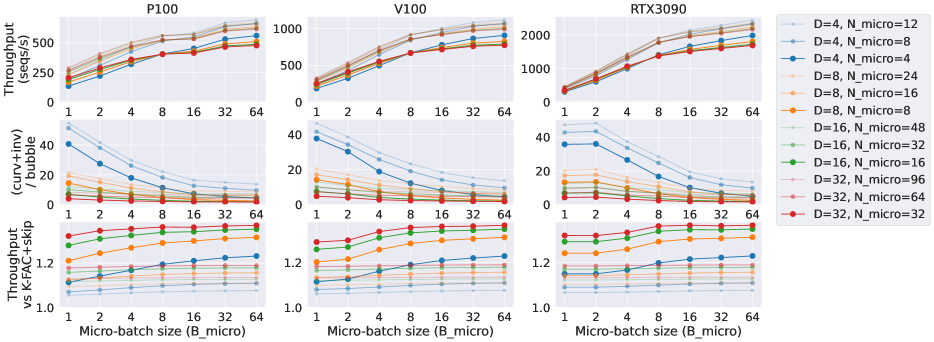
Figure 12: Modeled throughput (sequences/s) and (curvature+inversion)-bubble ratio of Chimera w/ $2$ pipelines w/ PipeFisher for $D$ BERT-Large blocks ($D\in\{4,8,16,32\}$, one block per pipeline stage) on an NVIDIA P100, V100, and RTX3090.

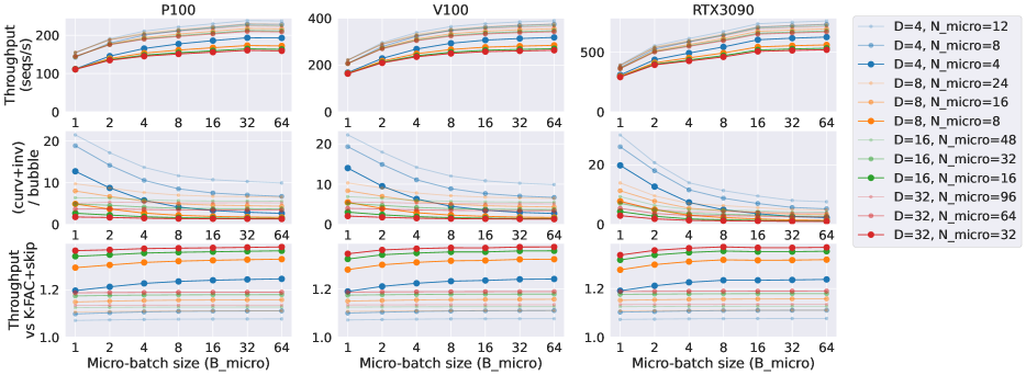
Figure 13: Modeled throughput (sequences/s) and (curvature+inversion)-bubble ratio of Chimera w/ $2$ pipelines w/ PipeFisher for $D$ T5-Base blocks ($D\in\{4,8,16,32\}$, one block per pipeline stage) on an NVIDIA P100, V100, and RTX3090.

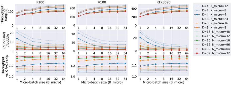
Figure 14: Modeled throughput (sequences/s) and (curvature+inversion)-bubble ratio of Chimera w/ $2$ pipelines w/ PipeFisher for $D$ T5-Large blocks ($D\in\{4,8,16,32\}$, one block per pipeline stage) on an NVIDIA P100, V100, and RTX3090.

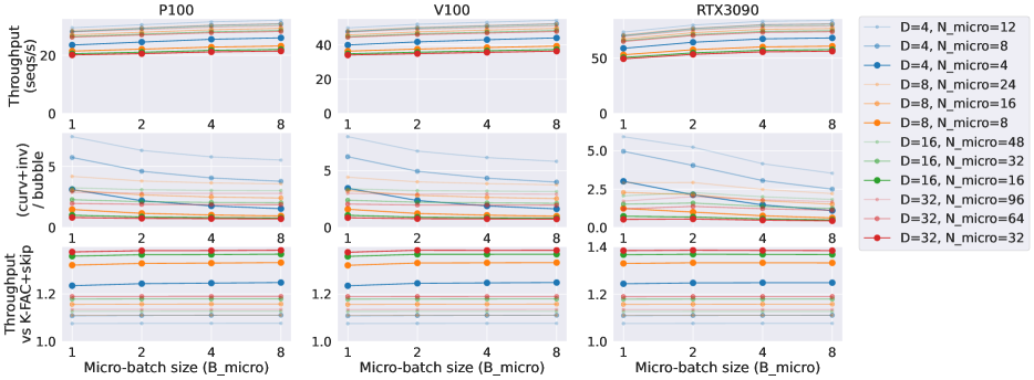
Figure 15: Modeled throughput (sequences/s) and (curvature+inversion)-bubble ratio of Chimera w/ $2$ pipelines w/ PipeFisher for $D$ OPT-125M blocks ($D\in\{4,8,16,32\}$, one block per pipeline stage) on an NVIDIA P100, V100, and RTX3090.

Figure	Architecture	Block class	Configuration
			$d_{model}$	$d_{ff}$	$h$	$S$
Figure 9, Figure 11	BERT-Base	BertLayer	768	3072	12	128
Figure 10, Figure 12	BERT-Large	BertLayer	1024	4096	16	128
Figure 13	T5-Base	T5Block	768	3072	12	512
Figure 14	T5-Large	T5Block	1024	4096	16	512
Figure 15	OPT-125M (Base)	OPTDecoderLayer	768	3072	12	2048
Figure 16	OPT-350M (Large)	OPTDecoderLayer	1024	4096	16	2048

Appendix B Experimental Settings

B.1 Training data

To prepare the 14 GB English Wikipedia Wikipedia , we follow the data preparation instruction provided by Microsoft. As described in the License information, “all original textual content is licensed under the GNU Free Documentation License (GFDL) and the Creative Commons Attribution-Share-Alike 3.0 License.” The Term of Use says “you may encounter material that you find offensive, erroneous, misleading, mislabeled, or otherwise objectionable.”

B.2 Training settings

We pretrain BERT-Base Devlin et al. (2019) on the English Wikipedia (Phase 1 only) by NVLAMB and K-FAC. For NVLAMB, we set mini-batch size 8,192, max sequence length 128, weight decay 0.01, base learning rate $6\cdot 10^{-3}$, total training steps 7,038, and linear learning rate warming up steps 2,000. The learning rate at the $t$-th step after warm-up is determined by the polynomial decay: $\eta_{t}=\mathrm{base\_lr}\times(1-t/\mathrm{total\_steps})^{0.5}$. For K-FAC, the same hyperparameters are used except that the number of learning rate warming up steps is reduced to 600, resulting in larger learning rates than NVLAMB until the 2,000th step. The pretraining loss versus the number steps is shown in Figure 5 (left). Figure 8 shows the learning rate schedule.

Setting the micro-batch size to 32 (maximum number of powers of 2 that can be placed on a P100 GPU) would require 256 GPUs to run training with mini-batch size 8,192. However, to reduce total GPU hours and energy and CO₂ overheads, we simulate this training by using 32 GPUs and accumulating the micro-batch gradient over 8 steps before updating parameters ($32\times 32\times 8=8,192$.)

In addition to this, the training is done using simple data parallelism without pipelines for reducing GPU hours. This is because the entire BERT-Base model fits into the P100 GPU device memory (16 GB), and in this case data parallelism without any model partitioning saves the most GPU hours on 32 GPUs in the GPU cluster we use (although it increases the communication cost of the allreduce of gradients for data parallelism.) While the target of model partitioning is a model that is too large to fit in the memory of a single device, our study simulates the effects of pipelining with relatively small Transformers (i.e. BERT-Base and -Large) compared to today’s GPU memory limitations. Yet, the same techniques, discussions, and benefits of pipelining (and PipeFisher) described in our study are applicable to even larger Transformers.

The choice of the parallel training strategy does not affect the convergence of NVLAMB as long as the micro-batch gradients are synchronized, which is the case in all of our experiments. For K-FAC, we use data- and inversion-parallel K-FAC (Figure 2 (ii,b)), and the curvature and inverse matrices are refreshed once in 10 steps. We assume this does not affect the convergence by PipeFisher because it refreshes the matrices more frequently (once in 5-10 steps) in this BERT-Base setup as described in Figure 5.

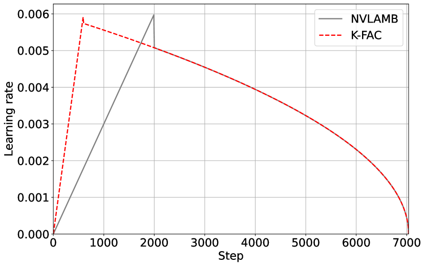
Figure 8: Learning rate schedule in Phase 1 pretraining of BERT-Base

B.3 Computational resources

We use a GPU cluster with NVIDIA P100 GPUs for all the experiments (except for Figure 11,12,13,14,15, and 16 where we use an NVIDIA V100 and a RTX3090 for micro benchmarks). For Phase 1 pretraining of BERT-Base, NVLAMB takes $\sim$7.4 hours while K-FAC takes $\sim$8.4 hours on 32 GPUs. To measure the time per step of PipeFisher, we only need to run about 10 steps of training on 4 (for Figure 3), 8 (for Figure 3 and 4), or 256 GPUs (for Figure 5), so the execution time is about 1-2 minutes, which is negligible compared to the training costs.

B.4 GPU utilization

We profile the pipeline steps by NVIDIA’s Nsight. We extract the CUDA activities (CUPTI_ACTIVITY_KIND_KERNEL) occurring within a work (either forward, backward, curvature, inversion, or precondition) from the profile results, and their start and end intervals are colored with the corresponding color in Figure 3 and 4. Therefore, the percentage of colored areas in each figure corresponds to the percentage of time that some kernel is being executed on the GPU, which we display as “GPU utilization”.

Appendix C Additional Discussion

C.1 Asynchronous pipeline methods

A synchronous pipeline method waits until the gradient calculations for all micro-batches in one mini-batch are completed at all pipeline stages before updating model parameters (pipeline flush) and starting the next pipeline. Hence, the pipeline flush makes most accelerator devices idle and creates the pipeline bubble. In asynchronous pipeline methods (e.g., PipeDream Narayanan et al. (2019), PipeDream-2BW Narayanan et al. (2021a)), on the other hand, no pipeline flush is performed and a different version of the model parameters (from 1 up to $D$ (the pipeline depth) steps old) are used at each stage to calculate the gradient. Therefore, pipeline bubbles are almost non-existent in asynchronous pipelines, but may reduce convergence in the gradient-based optimizer.

We propose PipeFisher as an extension to the synchronous pipeline methods for gaining an auxiliary benefit, i.e., improved convergence by K-FAC, in LLM training by “filling bubbles” with K-FAC work (i.e., curvature, inversion, and precondition work.) The model parameters ${\bm{\theta}}_{t}$ at the $t$-th step are updated by the fresh gradients ${\bm{g}}_{t}$ preconditioned by the stale curvature information: ${\bm{\theta}}_{t+1}={\bm{\theta}}_{t}-\eta\hat{{\bm{F}}}_{t-n}^{-1}{\bm{g}}_{t}$, where $n$ represents the number of additional steps (from 1 to $\sim$10, depending on the choice of the synchronous pipeline method, micro-batch size, and so on) taken to refresh the curvature information, and $\eta$ is the learning rate. We can also see an asynchronous pipeline method as a “filling bubbles” approach — the bubbles are filled by the gradient calculation (i.e., forward and backward work) with the stale model parameters, resulting in a higher throughput (number of tokens processed per unit time). The model parameters are then updated by the stale gradients: ${\bm{\theta}}_{t+1}={\bm{\theta}}_{t}-\eta{\bm{g}}_{t-m}$, where $m$ represents the number of the steps (from 1 up to $D$ steps, depending on the choice of the asynchronous pipeline method) to refresh the gradients.

C.2 Hyper-parameters for K-FAC

Compared to Adam, the only additional hyper-parameter of K-FAC is the frequency of matrix updates (i.e., curvature work and inversion work). With PipeFisher, the update frequency is no longer a hyperparameter, but is determined by network structure, number of pipeline stages, micro-batch size, and hardware. Therefore, there is no need to tune the frequency to make a trade-off between training time and convergence, and the achievable frequency by PipeFisher is much higher than previously feasible. As PipeFisher is the implementation of K-FAC to be performed more accurately (i.e., a higher frequency of matrix update) and cheaply (i.e., no extra communication, less memory consumption, no tuning of the frequency is required), it enables a cheaper hyper-paramerer search.

Figure 11: Modeled throughput (sequences/s) and (curvature+inversion)-bubble ratio of Chimera w/ $2$ pipelines w/ PipeFisher for $D$ BERT-Base blocks ($D\in\{4,8,16,32\}$, one block per pipeline stage) on an NVIDIA P100, V100, and RTX3090.

Figure 16: Modeled throughput (sequences/s) and (curvature+inversion)-bubble ratio of Chimera w/ $2$ pipelines w/ PipeFisher for $D$ OPT-350M blocks ($D\in\{4,8,16,32\}$, one block per pipeline stage) on an NVIDIA P100, V100, and RTX3090.

References

- Amari (1998) Amari, S.-i. Natural Gradient Works Efficiently in Learning. Neural Computation, 10(2):251–276, 1998.
- Anil et al. (2021) Anil, R., Gupta, V., Koren, T., Regan, K., and Singer, Y. Scalable Second Order Optimization for Deep Learning. arXiv preprint arXiv:2002.09018, 2021. URL http://arxiv.org/abs/2002.09018. arXiv: 2002.09018.
- Ba et al. (2017) Ba, J., Grosse, R., and Martens, J. Distributed second-order optimization using Kronecker-factored approximations. In International Conference on Learning Representations (ICLR), 2017. URL https://openreview.net/forum?id=SkkTMpjex.
- Brown et al. (2020) Brown, T. B., Mann, B., Ryder, N., Subbiah, M., Kaplan, J., Dhariwal, P., Neelakantan, A., Shyam, P., Sastry, G., Askell, A., Agarwal, S., Herbert-Voss, A., Krueger, G., Henighan, T., Child, R., Ramesh, A., Ziegler, D. M., Wu, J., Winter, C., Hesse, C., Chen, M., Sigler, E., Litwin, M., Gray, S., Chess, B., Clark, J., Berner, C., McCandlish, S., Radford, A., Sutskever, I., and Amodei, D. Language Models are Few-Shot Learners. In Advances in Neural Information Processing Systems, pp. 1877–1901, 2020.
- Chen et al. (2016) Chen, T., Xu, B., Zhang, C., and Guestrin, C. Training Deep Nets with Sublinear Memory Cost. arXiv preprint arXiv:1604.06174, 2016.
- Chowdhery et al. (2022) Chowdhery, A., Narang, S., Devlin, J., Bosma, M., Mishra, G., Roberts, A., Barham, P., Chung, H. W., Sutton, C., Gehrmann, S., Schuh, P., Shi, K., Tsvyashchenko, S., Maynez, J., Rao, A., Barnes, P., Tay, Y., Shazeer, N., Prabhakaran, V., Reif, E., Du, N., Hutchinson, B., Pope, R., Bradbury, J., Austin, J., Isard, M., Gur-Ari, G., Yin, P., Duke, T., Levskaya, A., Ghemawat, S., Dev, S., Michalewski, H., Garcia, X., Misra, V., Robinson, K., Fedus, L., Zhou, D., Ippolito, D., Luan, D., Lim, H., Zoph, B., Spiridonov, A., Sepassi, R., Dohan, D., Agrawal, S., Omernick, M., Dai, A. M., Pillai, T. S., Pellat, M., Lewkowycz, A., Moreira, E., Child, R., Polozov, O., Lee, K., Zhou, Z., Wang, X., Saeta, B., Diaz, M., Firat, O., Catasta, M., Wei, J., Meier-Hellstern, K., Eck, D., Dean, J., Petrov, S., and Fiedel, N. PaLM: Scaling Language Modeling with Pathways. arXiv preprint arXiv:2204.02311, 2022.
- Devlin et al. (2019) Devlin, J., Chang, M.-W., Lee, K., and Toutanova, K. BERT: Pre-training of Deep Bidirectional Transformers for Language Understanding. In Proceedings of the 2019 Conference of the North American Chapter of the Association for Computational Linguistics: Human Language Technologies, pp. 4171–4186, 2019.
- Duchi et al. (2011) Duchi, J., Hazan, E., and Singer, Y. Adaptive Subgradient Methods for Online Learning and Stochastic Optimization. Journal of Machine Learning Research, 12:2121–2159, 2011.
- Evci et al. (2020) Evci, U., Gale, T., Menick, J., Castro, P. S., and Elsen, E. Rigging the Lottery: Making All Tickets Winners. In Proceedings of International Conference on Machine Learning (ICML), 2020.
- Foret et al. (2021) Foret, P., Kleiner, A., Mobahi, H., and Neyshabur, B. Sharpness-Aware Minimization for Efficiently Improving Generalization. In International Conference on Learning Representations (ICLR), 2021. URL https://openreview.net/forum?id=6Tm1mposlrM.
- Griewank & Walther (2000) Griewank, A. and Walther, A. Algorithm 799: revolve: an implementation of checkpointing for the reverse or adjoint mode of computational differentiation. ACM Transactions on Mathematical Software, 26(1):19–45, March 2000. ISSN 0098-3500, 1557-7295. doi: 10.1145/347837.347846. URL https://dl.acm.org/doi/10.1145/347837.347846.
- Gupta et al. (2018) Gupta, V., Koren, T., and Singer, Y. Shampoo: Preconditioned Stochastic Tensor Optimization. In Proceedings of International Conference on Machine Learning (ICML), pp. 1842–1850, March 2018.
- Hochreiter & Schmidhuber (1997) Hochreiter, S. and Schmidhuber, J. Flat Minima. Neural Computation, 9(1):1–42, 1997.
- Huang et al. (2019) Huang, Y., Cheng, Y., Bapna, A., Firat, O., Chen, M. X., Chen, D., Lee, H., Ngiam, J., Le, Q. V., Wu, Y., and Chen, Z. GPipe: Efficient Training of Giant Neural Networks using Pipeline Parallelism. In Advances in Neural Information Processing Systems, pp. 103–112, July 2019.
- Keskar et al. (2017) Keskar, N. S., Mudigere, D., Nocedal, J., Smelyanskiy, M., and Tang, P. T. P. On Large-Batch Training for Deep Learning: Generalization Gap and Sharp Minima. In International Conference on Learning Representations (ICLR), 2017. URL https://openreview.net/forum?id=H1oyRlYgg.
- Kirkpatrick et al. (2017) Kirkpatrick, J., Pascanu, R., Rabinowitz, N., Veness, J., Desjardins, G., Rusu, A. A., Milan, K., Quan, J., Ramalho, T., Grabska-Barwinska, A., Hassabis, D., Clopath, C., Kumaran, D., and Hadsell, R. Overcoming catastrophic forgetting in neural networks. Proceedings of the national academy of sciences, 114(13):3521–3526, 2017.
- Li & Hoefler (2021) Li, S. and Hoefler, T. Chimera: Efficiently Training Large-Scale Neural Networks with Bidirectional Pipelines. In Proceedings of the International Conference for High Performance Computing, Networking, Storage and Analysis, 2021.
- Martens (2020) Martens, J. New Insights and Perspectives on the Natural Gradient Method. Journal of Machine Learning Research, 21(146):1–76, 2020.
- Martens & Grosse (2015) Martens, J. and Grosse, R. Optimizing Neural Networks with Kronecker-factored Approximate Curvature. In Proceedings of International Conference on Machine Learning (ICML), pp. 2408–2417, 2015.
- Narayanan et al. (2019) Narayanan, D., Harlap, A., Phanishayee, A., Seshadri, V., Devanur, N. R., Ganger, G. R., Gibbons, P. B., and Zaharia, M. PipeDream: generalized pipeline parallelism for DNN training. In Proceedings of the 27th ACM Symposium on Operating Systems Principles, pp. 1–15, Huntsville Ontario Canada, October 2019. ACM. ISBN 978-1-4503-6873-5. doi: 10.1145/3341301.3359646. URL https://dl.acm.org/doi/10.1145/3341301.3359646.
- Narayanan et al. (2021a) Narayanan, D., Phanishayee, A., Shi, K., Chen, X., and Zaharia, M. Memory-Efficient Pipeline-Parallel DNN Training. In International Conference on Machine Learning (ICML), pp. 7937–7947, 2021a.
- Narayanan et al. (2021b) Narayanan, D., Shoeybi, M., Casper, J., LeGresley, P., Patwary, M., Korthikanti, V. A., Vainbrand, D., Kashinkunti, P., Bernauer, J., Catanzaro, B., Phanishayee, A., and Zaharia, M. Efficient Large-Scale Language Model Training on GPU Clusters Using Megatron-LM. In Proceedings of the International Conference for High Performance Computing, Networking, Storage and Analysis, 2021b.
- Osawa et al. (2019) Osawa, K., Tsuji, Y., Ueno, Y., Naruse, A., Yokota, R., and Matsuoka, S. Large-Scale Distributed Second-Order Optimization Using Kronecker-Factored Approximate Curvature for Deep Convolutional Neural Networks. In IEEE Conference on Computer Vision and Pattern Recognition (CVPR), pp. 12359–12367, 2019.
- Osawa et al. (2022) Osawa, K., Tsuji, Y., Ueno, Y., Naruse, A., Foo, C.-S., and Yokota, R. Scalable and Practical Natural Gradient for Large-Scale Deep Learning. IEEE Transactions on Pattern Analysis and Machine Intelligence, 44(1):404–415, 2022.
- Pan et al. (2020) Pan, P., Swaroop, S., Immer, A., Eschenhagen, R., Turner, R. E., and Khan, M. E. Continual Deep Learning by Functional Regularisation of Memorable Past. In Advances in Neural Information Processing Systems, pp. 4453–4464, 2020.
- Pascanu & Bengio (2014) Pascanu, R. and Bengio, Y. Revisiting Natural Gradient for Deep Networks. In International Conference on Learning Representations (ICLR), 2014. URL https://openreview.net/forum?id=vz8AumxkAfz5U.
- Paszke et al. (2019) Paszke, A., Gross, S., Massa, F., Lerer, A., Bradbury, J., Chanan, G., Killeen, T., Lin, Z., Gimelshein, N., Antiga, L., Desmaison, A., Kopf, A., Yang, E., DeVito, Z., Raison, M., Tejani, A., Chilamkurthy, S., Steiner, B., Fang, L., Bai, J., and Chintala, S. PyTorch: An Imperative Style, High-Performance Deep Learning Library. In Advances in Neural Information Processing Systems (NeurIPS), pp. 8026–8037, 2019.
- Pauloski et al. (2020) Pauloski, J. G., Zhang, Z., Huang, L., Xu, W., and Foster, I. T. Convolutional Neural Network Training with Distributed K-FAC. In Proceedings of the International Conference for High Performance Computing, Networking, Storage and Analysis, 2020.
- Pauloski et al. (2021) Pauloski, J. G., Huang, Q., Huang, L., Venkataraman, S., Chard, K., Foster, I., and Zhang, Z. KAISA: An Adaptive Second-Order Optimizer Framework for Deep Neural Networks. In Proceedings of the International Conference for High Performance Computing, Networking, Storage and Analysis, 2021. doi: 10.1145/3458817.3476152.
- Pauloski et al. (2022) Pauloski, J. G., Huang, L., Xu, W., Chard, K., Foster, I., and Zhang, Z. Deep Neural Network Training with Distributed K-FAC. IEEE Transactions on Parallel and Distributed Systems, pp. 1–1, 2022. ISSN 1558-2183. doi: 10.1109/TPDS.2022.3161187. Conference Name: IEEE Transactions on Parallel and Distributed Systems.
- Pearlmutter (1994) Pearlmutter, B. A. Fast Exact Multiplication by the Hessian. Neural Computation, 6(1):147–160, January 1994. ISSN 0899-7667, 1530-888X. doi: 10.1162/neco.1994.6.1.147. URL http://www.mitpressjournals.org/doi/10.1162/neco.1994.6.1.147.
- Rajbhandari et al. (2020) Rajbhandari, S., Rasley, J., Ruwase, O., and He, Y. ZeRO: Memory Optimization Towards Training A Trillion Parameter Models. In Proceedings of the International Conference for High Performance Computing, Networking, Storage and Analysis, 2020.
- Rajbhandari et al. (2021) Rajbhandari, S., Ruwase, O., Rasley, J., Smith, S., and He, Y. ZeRO-Infinity: Breaking the GPU Memory Wall for Extreme Scale Deep Learning. In Proceedings of the International Conference for High Performance Computing, Networking, Storage and Analysis. arXiv, 2021.
- Ueno et al. (2020) Ueno, Y., Osawa, K., Tsuji, Y., Naruse, A., and Yokota, R. Rich Information is Affordable: A Systematic Performance Analysis of Second-order Optimization Using K-FAC. In Proceedings of the 26th ACM SIGKDD International Conference on Knowledge Discovery & Data Mining, pp. 2145–2153, Virtual Event CA USA, August 2020. ACM. ISBN 978-1-4503-7998-4. doi: 10.1145/3394486.3403265. URL https://dl.acm.org/doi/10.1145/3394486.3403265.
- Vaswani et al. (2017) Vaswani, A., Shazeer, N., Parmar, N., Uszkoreit, J., Jones, L., Gomez, A. N., Kaiser, L., and Polosukhin, I. Attention Is All You Need. In Advances in Neural Information Processing Systems, pp. 5998–6008, 2017.
- (36) Wikipedia. Wikimedia Downloads. URL https://dumps.wikimedia.org/.
- You et al. (2020) You, Y., Li, J., Reddi, S., Hseu, J., Kumar, S., Bhojanapalli, S., Song, X., Demmel, J., and Hsieh, C.-J. Large Batch Optimization for Deep Learning: Training BERT in 76 minutes. In International Conference on Learning Representations (ICLR), 2020. URL https://openreview.net/forum?id=Syx4wnEtvH.