newfloatplacementnewfloatnamenewfloatfileextnewfloatwithin

Conditional Gradient Methods

Gábor Braun        Alejandro Carderera        Cyrille W. Combettes
Hamed Hassani Amin Karbasi Aryan Mokhtari Sebastian Pokutta

Draft: Please send comments/suggestions to frank.wolfe.book@gmail.com.

1 Introduction

You can’t improve what you don’t measure. Indeed, many scientific and engineering methods rely on the simple idea of measuring a phenomenon, such as the capacity of a communication network, the position of a robotic arm, etc, and then making small improvements towards a pre-defined goal, such as decreasing the communication error or changing the position of the robotic arm to grab an object. More often than not, in order to update such systems reliably we need to be mindful of various constraints along the path of improvements, for example, the energy consumption of the communication system should never be above a threshold, or to meet the safety measures for the robotic arm some configurations cannot be reached. Maximizing the utility (or minimizing the cost) subject to feasibility constraints is the essence of constrained optimization problems.

With the emergence of machine learning and artificial intelligence applications, constrained optimization has become an integral part of the entire training and inference pipeline. Examples include signal recovery with a sparsity constraint [81, 48], matrix completion with a rank constraint [46], exploration with safety constraints [235], adversarial attacks with noise constraints [113], experimental design with a budget constraint [209], optimal transport with a probability polytope constraint [254], and submodular optimization with a matroid constraint [45], to just name a few.

Augustin-Louis Cauchy

I’ll restrict myself here to outlining the principles underlying [my method], with the intention to come again over the same subject, in a paper to follow.

English translation, [54]

Figure 1: When proposing gradient descent, Cauchy was apparently unhappy with the lack of rigor, as the excerpt shows. As often the case, there is no follow-up paper! [156].

At a bird’s eye view, constrained optimization problems involve minimizing an objective function $f$ (or equivalently maximizing a utility function $-f$) over a feasible region $\mathcal{X}$. In most machine learning applications (including the ones just mentioned), $f$ measures the discrepancy between the model we aim to develop and the underlying data. Typically, optimization methods start from an initial point and aim to improve the solution via local steps/measurements. What kind of information they use determines how fast they might converge to a desirable solution. For instance, at the lowest level, an optimization method may only have access to a limited number of function evaluations at each step (so called the zeroth-order information). Typically, it is feasible to obtain higher order information such as the rate of change, i.e., gradient, which leads to a slew of algorithms that exploit this information (i.e., the vector that indicates the direction of largest change of $f$) in an intelligent fashion. These algorithms are called first-order methods. Of course, we can think of developing methods that use not only the rate of change, but also the rate of the rate of change (i.e., so called second-order methods), or the rate of the rate of the rate of change (so called third-order methods), etc. Nothing prevents us from doing that except the computational cost. As the data points become high-dimensional, the cost of computing higher derivatives becomes prohibitive. This is why the first-order algorithms, which only utilize the gradient of the objective function to build each iterate, provide a good compromise between progress and cost per function access and have thus become the workhorse of most machine learning applications. This survey is mainly focused on first-order methods.

Yann LeCun [@ylecun] (2022, June 5) [Tweet] Twitter
https://twitter.com/ylecun/status/1533451405167669249

Figure 2: Recently, academics have started using Twitter (with each message containing up to 280 characters) to settle differences. Ironically, the medium is hardly optimized for such debates.

As we mentioned earlier, most first-order algorithms move along adequately chosen directions that typically attempt to decrease the value of the objective function. However note that such methods may easily leave the feasible region, leading to an infeasible solution. Traditionally, projected gradient descent algorithms have been the method of choice for constrained optimization. Some even attributed the huge success of machine learning methods to the gradient descent algorithm (see Figure 2 for a post starting a comprehensive debate).

However, in recent years, with the surge of large data and complicated constraints, it has become evident that such methods may hugely suffer from the cost of the projection operation. Indeed, it is known that for many practical problems, it is practically infeasible to compute the projection operator. As a result, there has been a lot of interest in optimization methods that do not require any projection, so-called projection-free methods, which resort to simpler operations with the aim of never leaving the feasible domain.

1 Why Frank–Wolfe algorithms?

Recall that the projection operator maps a point $y$ to a closest point in some set $\mathcal{X}$:

$$\operatorname*{argmin}_{x\in\mathcal{X}}\mathinner{{}\lVert x-y\rVert}_{2}\quad\text{(projection)},$$ (1)

which can be implemented via a quadratic program. To avoid projections, we should consider simpler mathematical programs that are arguably easier to implement. This survey is about methods that replace the projection with a Linear Minimization Oracle (LMO), i.e.,

$$\operatorname*{argmin}_{x\in\mathcal{X}}\mathinner{{}\langle x,y\rangle}\quad\text{(linear minimization)}.$$ (2)

When the feasible region $\mathcal{X}$ admits fast linear optimization, the method of choice becomes the Frank–Wolfe algorithm [97], also known as Conditional Gradient algorithm [157], a simple projection-free first-order algorithm for constrained convex optimization problems, requiring a comparable number of linear minimizations as the number of projections needed by projection-based first-order methods. Thus the actual cost of these projection-free methods is much lower. Frank–Wolfe methods avoid projection by moving towards but not beyond an extreme point obtained via linear minimization, which obviously ensures staying within the feasible region $\mathcal{X}$. One of the most striking examples highlighting the advantage of projection-free methods is probably the spectrahedron, where projections require the computation of a full SVD (singular value decomposition), whereas for the LMO the computation of the largest eigenvector is enough, e.g., via the Lanczos method. Some other practical problems for which projections are costly are matrix completion [98], network routing [155], and finding a maximum matching [163].

Table 1: Complexities of linear minimizations and projections on some convex sets up to an additive error $\varepsilon$ in the Euclidean norm. When $\varepsilon$ is missing, there is no additive error. The $\tilde{\mathcal{O}}$ hides polylogarithmic factors in the dimensions and polynomial factors in constants related to the distance to the optimum. For the nuclear norm ball, i.e., the spectrahedron, $\nu$ denotes the number of non-zero entries and $\sigma_{1}$ denotes the top singular value of the projected matrix.

Set	Linear minimization	Projection
$n$-dimensional $\ell_{p}$-ball, $p\neq 1,2,\infty$	$\mathcal{O}(n)$	$\tilde{\mathcal{O}}(n/\varepsilon^{2})$
Nuclear norm ball of $n\times m$ matrices	$\mathcal{O}(\nu\ln(m+n)\sqrt{\sigma_{1}}/\sqrt{\varepsilon})$	$\mathcal{O}(mn\min\{m,n\})$
Flow polytope on a graph with $m$ vertices and $n$ edges with capacity bound on edges	$\mathcal{O}((n\log m)(n+m\log m))$	$\mathcal{O}(n^{4}\log n)$
Birkhoff polytope ($n\times n$ doubly stochastic matrices)	$\mathcal{O}(n^{3})$	$\tilde{\mathcal{O}}(n^{2}/\varepsilon^{2})$

To provide an (incomplete) comparison, in Table 1 we present complexities of linear minimization and projection onto the $\ell_{p}$-ball, the nuclear norm ball (also called spectrahedron), the flow polytope, and the Birkhoff polytope (see Example 3.9). The matching polytope is not included in the table, as no (either theoretical or practical) efficient projection algorithm is known, however it has a practical, efficient polynomial time linear minimization algorithm [89] despite all LP formulations having an exponential number of inequalities (in the number of nodes of the underlying graph). The table is from [68] except the complexities for the flow polytope, which are from original research papers [252, 196].

Another important property of conditional gradient algorithms is the way the iterates are usually built, namely as convex combinations of extremal points (e.g., vertices in the case of polytopes). In fact, most Frank–Wolfe algorithms add (at most) one extremal point per iteration to the representation. This typically leads to sparse iterates, which is important in many applications. A classical example is optimization over the nuclear norm ball, where in each iteration a single rank-$1$ matrix is added, so that after $t$ iterations, we obtain an approximation or solution with rank at most $t+1$ (see Examples 3.19, 3.22 and 4.34). Another classical example is the approximate Carathéodory problem, where a point contained in a compact convex set is to be approximated as a convex combination of a small number of extremal points and the object of study here is the sparsity vs. approximation error trade-off, see Example 5.14.

2 Organization and how to read this survey

The purpose of this survey is to serve both as a gentle introduction and a coherent overview of state-of-the-art algorithms. More specially, we will cover what is this class of optimization methods, why you should care about them, and how you can run an appropriate algorithm, from a plethora of variants, for your specific optimization problem. The selection of the material has been guided by the principle of highlighting crucial ideas as well as presenting new approaches that we believe might become important in the future, with ample citations even of old works imperative in the development of newer methods. Yet, our selection is sometimes biased, and need not reflect consensus of the research community, and we have certainly missed recent important contributions. After all the research area of Frank–Wolfe algorithms is very active, making it a moving target. We apologize sincerely in advance for any such distortions and we fully acknowledge: We stand on the shoulder of giants.

This survey contains three main parts. Chapter 2 addresses the basics of the Frank–Wolfe algorithm and provides an overview of the basic methodology, lower bounds, and some variants that are to be considered standard by now. In Chapter 3 we consider more recent improvements of conditional gradients, mostly better convergence rates and more generally faster algorithms. In Chapter 4 we address the large-scale settings, where we cover the stochastic case, decentralized optimization, and online learning. Finally, Chapter 5 contains a few related methods that are substantially different from core variants of Frank–Wolfe algorithms and a number of applications.

For readers interested in understanding the basics, we highly recommend Chapter 2 as it contains much of the core algorithmic ideas and is a prerequisite for the later ones. Chapters 3 and 4 are quite independent of each other and contain more advanced topics, including very recent results. We have also tried to include computational comparisons wherever reasonable and provide some practical advice on how to run different algorithms.

A recent useful building block for implementations, which we are not using for legacy reasons, is the FrankWolfe.jl Julia package (released under MIT license and available at https://github.com/ZIB-IOL/FrankWolfe.jl), which provides high-performance state-of-the-art implementations of many Frank–Wolfe methods and as such does not only serve as a natural benchmark or baseline but also facilitates the development of novel Frank–Wolfe methods by providing a clean and hardened framework similar to what, e.g., tensorflow, pytorch, or scikit-learn do for machine learning.

3 A bit of history

Frank–Wolfe algorithms (a.k.a. conditional gradients) have a very long history and we only mention some of the key works along the way. In particular, recreating the timeline is not without difficulty given sometimes prolonged publication delays, hence minor inaccuracies are inevitable.

The original algorithm is due to [97] with later generalizations due to [157]. Initial convergence guarantees for the vanilla method were established back then. A first lower bound to the achievable convergence rate was then obtained in [49]. In particular, the zigzagging phenomenon that fundamentally limits the rate of convergence of the vanilla Frank–Wolfe algorithm became apparent and various extensions of the base method were explored. One particular suggestion was the Away-Step Frank–Wolfe algorithm by [260], albeit at this point in time without any established convergence rate. Another important variant, which came to be known as the Fully-Corrective Frank–Wolfe algorithm, was presented by [126]. Other important works considered specific convergence rates regimes [87] and in particular open-loop step-sizes [86]. Almost ten years later [114] presented a very nice argument demonstrating that when the optimal solution is contained in the interior, and the function is strongly convex then the vanilla Frank–Wolfe algorithm with line search converges linearly. This result also implied that after a certain number of iterations (effectively after having identified the optimal face), for strongly convex functions Wolfe’s Away-Step Frank–Wolfe algorithm converges linearly, indicating that global linear convergence for strongly convex functions might be achievable; however it would take another 30 years to actually prove this.

Then it stayed relatively quiet around conditional gradient methods for about 27 years, interspersed with isolated but no less important results such as, e.g., coreset constructions via the Frank–Wolfe algorithm in [65, 14, 15]. Around 2013, there was a sudden surge of new results for Frank–Wolfe methods [131, 146, 149, 103] re-analyzing some of the former results and providing unifying perspectives. The stream of new results in that area has been uninterrupted since then. Some of the highlights include faster convergence rates over structured sets [104, see, e.g.,] and global linear convergence proofs for (modifications of) conditional gradients [105], including for Wolfe’s Away-Step Frank–Wolfe algorithm [147]. In the following we will present many more results, up to today, as well as put the classical ones into context.

4 Overview of conditional gradient algorithms

As mentioned earlier conditional algorithms are iterative algorithms: i.e., they generate a sequence of feasible solutions called iterates, with each iterate intended to improve on the previous one. The core building block is the Frank–Wolfe step: at each iterate move a bit towards an extreme point that minimizes the linear approximation of the objective function given by its gradient. This move leads to the next iterate. The extensions and variants of the original Frank–Wolfe algorithm fall broadly into the following four categories.

Alternative descent directions.

A descent direction is the direction between successive iterates. The first category combines the Frank–Wolfe step with other ways of finding an improving solution or descent directions typically maintaining projection-freeness, in particular for structured feasible regions (such as, e.g., polytopes). The Away-step Frank–Wolfe algorithm and the Pairwise-step Frank–Wolfe algorithm are quite unique in this category by adding simple new steps designed for the Frank–Wolfe setting overcoming known convergence obstacles (e.g., the zigzagging phenomenon). An extreme variant is for example the Fully-Corrective Frank–Wolfe algorithm which optimizes over a local subproblem to determine the best direction.

Adaptivity.

The second category improves parts of the Frank–Wolfe algorithm by, e.g., deliberately avoiding problem parameter estimations or arbitrary fixed quantities, e.g., for the step size, i.e., how far to go into the descent direction. Such parameters are a source of suboptimal performance in practice for all kinds of algorithms, not just conditional gradients. The aim is to derive adaptive algorithms that, e.g., adjust to the local behavior, rather than using some loose global estimates for these parameters. This includes adaptive step-size strategies that approximate the local smoothness constant but also variants that automatically adapt to additional problem structure, both in the objective function (e.g., sharpness) or the feasible region (e.g., uniform convexity).

Other Oracles.

A third category’s goal is to replace even the most basic building blocks of Frank–Wolfe algorithms (function access, linear minimization) treated as oracles with cheaper or stronger variants. Cheaper variants include, e.g., lazy algorithms allowing a large error in linear minimization, stochastic algorithms using stochastic gradients (cheap gradient approximations) instead of the true gradients, or distributed algorithms where function access have significant communication cost and hence amortization schemes are devised. On the other hand, stronger oracles include the nearest extreme point oracle, which solves a more complicated problem but delivers finer sparsity and convergence guarantees.

Applicability.

Finally, there has been a significant amount of work for making Frank–Wolfe methods more broadly applicable, e.g., for a wider class of objective functions (e.g., generalized self-concordant, non-smooth, or composite functions) and feasible regions (e.g., infinite dimensional domains).

As a note on naming conventions, while in the literature often “Frank–Wolfe” and “conditional gradients” are used interchangeably, in this survey a “Frank–Wolfe algorithm” is a core variant of the original algorithm, while a “conditional gradient algorithm” differs significantly from the original version. This classification reflects the opinion of the authors in some corner cases. However, we use the original algorithm names for consistency with the literature, even if the classification requires otherwise.

5 Basics and notation

The basic setup is the following, which some later sections augment or replace. Given a differentiable function $f\colon\mathcal{X}\to\mathbb{R}$ over a compact (i.e., closed and bounded) convex domain $\mathcal{X}$, our goal is to find a point in $\mathcal{X}$ that minimizes the value of $f$ up to a given additive error. (The definition of convexity is recalled below.) We do this armed with the following two oracles as the only methods directly accessing the objective function $f$ and the feasible region $\mathcal{X}$. As mentioned above, these oracles provide a balanced choice between cost and useful information in many settings. Note that here and in the following, as our algorithms don’t need access to function values outside the feasible region, unless otherwise stated, we implicitly make the simplifying assumption that the domain of the function is the feasible region $\mathcal{X}$.

The first oracle, called the First-Order Oracle (denoted as FOO and shown in Oracle 1), gives information about the function $f$: when queried with a point $x\in\mathcal{X}$, FOO returns the function value $f(x)$ (i.e., zero-order information) and the gradient $\nabla f(x)$ of $f$ at $x$.

Algorithm 1 First-Order Oracle for $f$ (FOO)

0   Point $x\in\mathcal{X}$

0   $\nabla f(x)$ and $f(x)$

The second oracle, called a Linear Minimization Oracle (denoted as LMO and shown in Oracle 2), gives information about the domain $\mathcal{X}$: when queried with a linear function $c$, the LMO returns an extreme point $v\in\mathcal{X}$ minimizing $c$, in particular, $v=\operatorname*{argmin}_{x\in\mathcal{X}}\mathinner{{}\langle c,x\rangle}$. Note that $v$ is not necessarily unique, however as here, we slightly abuse notation for simplicity. (Extreme points are often called atoms in the context of conditional gradient algorithms).

Algorithm 2 Linear Minimization Oracle over $\mathcal{X}$ (LMO)

0   Linear objective $c$

0   $v=\operatorname*{argmin}_{x\in\mathcal{X}}\mathinner{{}\langle c,x\rangle}$

We now review convexity and related properties allowing for better algorithms than evaluating the objective function at every feasible point by brute force.

Definition 1.1 (Convex set).

A set $\mathcal{X}\subseteq\mathbb{R}^{n}$ is convex if for every points $x,y\in\mathcal{X}$ the segment between $x$ and $y$ is contained in $\mathcal{X}$, that is,

$$\gamma x+(1-\gamma)y\in\mathcal{X}\quad\text{for all $0\leq\gamma\leq 1$.}$$ (3)

A convex set $\mathcal{X}$ is full dimensional if it has a non-empty interior, or equivalently if it is not contained in any proper affine subspace of $\mathbb{R}^{n}$.

Definition 1.2 (Convex function).

A function $f\colon\mathcal{X}\to\mathbb{R}$ is convex if its domain $\mathcal{X}$ is convex and

$$f\bigl{(}\gamma x+(1-\gamma)y\bigr{)}\leq\gamma f(x)+(1-\gamma)f(y)\quad\text{for all }x,y\in\mathcal{X},\ 0\leq\gamma\leq 1.$$ (4)

If $f$ is differentiable then it is convex if and only if

$$f(y)-f(x)\geq\mathinner{{}\langle\nabla f(x),y-x\rangle}\quad\text{for all }x,y\in\mathcal{X},$$ (5)

or equivalently $f(y)-f(x)\leq\mathinner{{}\langle\nabla f(y),y-x\rangle}$.

Convex functions have the nice property that local minima are always global minima. Optimization algorithms often rely on good local approximation of the objective function, and therefore the following two properties have been useful for finding a quadratic approximation. For simplicity we formulate the properties only for differentiable functions. See Section 5.2 below for further inequalities for these properties. See [115] for generalization of these properties, which in most results can replace the above ones.

Definition 1.3 (Strongly convex function).

A differentiable function $f\colon\mathcal{X}\to\mathbb{R}$ is $\mu$-strongly convex if

$$f(y)-f(x)\geq\mathinner{{}\langle\nabla f(x),y-x\rangle}+\frac{\mu}{2}\mathinner{{}\lVert y-x\rVert}^{2}\quad\text{for all }x,y\in\mathcal{X}.$$ (6)

Definition 1.4 (Smooth function).

A differentiable function $f\colon\mathcal{X}\to\mathbb{R}$ is $L$-smooth if for all $x,y\in\mathcal{X}$

$$f(y)-f(x)\leq\mathinner{{}\langle\nabla f(x),y-x\rangle}+\frac{L}{2}\mathinner{{}\lVert y-x\rVert}^{2}\quad\text{for all }x,y\in\mathcal{X}.$$ (7)

Note that in optimization theory smoothness has a different meaning than in topology or differential geometry, where a smooth function means an infinitely many times differentiable function; older papers also use the term bounded convexity for smoothness.

An important application of smoothness is estimating the decrease in function value of $f$ when improving a solution $x$ via moving in an arbitrary direction $d$, i.e., estimating $f(x)-f(x-\gamma d)$, where $\gamma$ is called the step size, and $x-\gamma d$ is the improved solution. This is formulated in the following lemma, which is mostly useful when moving in a descent direction, i.e., when $\mathinner{{}\langle\nabla f(x),d\rangle}>0$. In applications, the upper bound on the step size $\gamma$ required by the lemma will usually be ensured by force, i.e., choosing $\gamma$ as the minimum of the upper bound and a desired value. Conditional gradient algorithms typically choose $d=v-x$ for some feasible point $v$.

Lemma 1.5 (Progress lemma from smoothness).

Let $f$ be an $L$-smooth function. Define $y=x-\gamma d$, where $d$ is an arbitrary vector (i.e., a direction). Then if $y$ is in the domain of $f$

$$f(x)-f(y)\geq\frac{\mathinner{{}\langle\nabla f(x),d\rangle}}{2}\cdot\gamma\quad\text{for}\quad 0\leq\gamma\leq\frac{\mathinner{{}\langle\nabla f(x),d\rangle}}{L\mathinner{{}\lVert d\rVert}^{2}}.$$ (8)

Proof.

Equation (8) follows easily from Definition 1.4:

$$\begin{split}f(x)-f(y)\geq\gamma\mathinner{{}\langle\nabla f(x),d\rangle}-\gamma^{2}\frac{L\mathinner{{}\lVert d\rVert}^{2}}{2}&\geq\gamma\mathinner{{}\langle\nabla f(x),d\rangle}-\gamma\frac{\mathinner{{}\langle\nabla f(x),d\rangle}}{L\mathinner{{}\lVert d\rVert}^{2}}\cdot\frac{L\mathinner{{}\lVert d\rVert}^{2}}{2}\\ &=\frac{\mathinner{{}\langle\nabla f(x),d\rangle}}{2}\cdot\gamma,\end{split}$$ (9)

where we have used the definition of $y$ and the bound on the step size $\gamma$. ∎

Remark 1.6 (Typical application of Lemma 1.5).

In applications of Lemma 1.5 there will be usually an upper bound $\gamma_{\max}$ on the step size $\gamma$ to ensure that $y$ lies in the feasible region. The step size will be chosen to optimize the progress bound: $\gamma\stackrel{{\scriptstyle\textnormal{\scriptsize def}}}{{=}}\min\{\mathinner{{}\langle\nabla f(x),d\rangle}\mathbin{/}(L\mathinner{{}\lVert d\rVert}^{2}),\gamma_{\max}\}$, so that the progress lower bound becomes

$$f(x)-f(y)\geq\frac{\mathinner{{}\langle\nabla f(x),d\rangle}}{2}\cdot\min\left\{\gamma_{\max},\frac{\mathinner{{}\langle\nabla f(x),d\rangle}}{L\mathinner{{}\lVert d\rVert}^{2}}\right\}.$$

In fact for most steps (usually except for a few early iterations), we have $\frac{\mathinner{{}\langle\nabla f(x),d\rangle}}{L\mathinner{{}\lVert d\rVert}^{2}}\leq\gamma_{\max}$, so that the above reduces to

$$f(x)-f(y)\geq\frac{\mathinner{{}\langle\nabla f(x),d\rangle}^{2}}{2L\mathinner{{}\lVert d\rVert}^{2}}.$$

Sometimes we will also work with a lower bound $\phi$ with $\mathinner{{}\langle\nabla f(x),d\rangle}\geq\phi$ and in this case, the progress estimation becomes

$$f(x)-f(y)\geq\frac{\phi}{2}\cdot\min\left\{\gamma_{\max},\frac{\phi}{L\mathinner{{}\lVert d\rVert}^{2}}\right\}.$$

5.1 Notation

Now we introduce notation used throughout this survey. Whenever the domain is a polytope, i.e., the convex hull of finitely many points, we will use $P$ instead of $\mathcal{X}$. The domain $\mathcal{X}$ will always be a subset of a finite dimensional vector space $\mathbb{R}^{n}$. For convenience, we equip $\mathbb{R}^{n}$ with a non-degenerate bilinear form $\mathinner{{}\langle\cdot,\cdot\rangle}\colon\mathbb{R}^{n}\times\mathbb{R}^{n}\to\mathbb{R}$, so that every linear function $\mathbb{R}^{n}\to\mathbb{R}$ is uniquely represented by a vector $c\in\mathbb{R}^{n}$ as $\mathinner{{}\langle c,\cdot\rangle}$. In particular, the gradient $\nabla f(x)$ of a function at $x$ represents the derivative $f^{\prime}(x)$ at $x$ as a linear function, i.e., $f^{\prime}(x)z=\mathinner{{}\langle\nabla f(x),z\rangle}$. We shall further equip $\mathbb{R}^{n}$ with a norm $\mathinner{{}\lVert\cdot\rVert}$ but for vectors representing linear functions we will use the dual norm $\mathinner{{}\lVert\cdot\rVert}_{*}$. Thus $\lvert\mathinner{{}\langle c,x\rangle}\rvert\leq\mathinner{{}\lVert c\rVert}_{*}\cdot\mathinner{{}\lVert x\rVert}$ for example. As a consequence, even though $\nabla f(x)$ depends on the choice of the inner product $\mathinner{{}\langle\cdot,\cdot\rangle}$, expressions like $\mathinner{{}\langle\nabla f(x),z\rangle}$ and $\mathinner{{}\lVert\nabla f(x)\rVert}_{*}$ are independent of it.

Readers unfamiliar with norms can restrict to the most common choice: the Euclidean norm $\mathinner{{}\lVert x\rVert}_{2}=\sqrt{\sumop\slimits@_{i=1}^{n}x_{i}^{2}}$, which is its own dual norm, for which we always use the standard scalar product $\mathinner{{}\langle x,y\rangle}=\sumop\slimits@_{i=1}^{n}x_{i}y_{i}$ as inner product. In this case our definition of gradient reduces to the usual one.

When $\mathinner{{}\langle\cdot,\cdot\rangle}$ is the standard scalar product, for any symmetric positive definite matrix $H$, we use $\mathinner{{}\lVert x\rVert}_{H}$ to define the matrix norm defined by $H$, that is, $\mathinner{{}\lVert x\rVert}_{H}=\sqrt{\mathinner{{}\langle x,Hx\rangle}}$. In this survey we will also use the $\ell_{p}$-norm (also called $p$-norm): $\mathinner{{}\lVert x\rVert}_{p}=\sqrt[p]{\sumop\slimits@_{i=1}^{n}\lvert x_{i}\rvert^{p}}$ for $1\leq p\leq\infty$. Recall that $\mathinner{{}\lVert x\rVert}_{\infty}=\max_{i=1}^{n}\lvert x_{i}\rvert$. An $\ell_{p}$-ball is a ball in the $\ell_{p}$-norm. The diameter $D$ of a set $\mathcal{X}$ is $D\stackrel{{\scriptstyle\textnormal{\scriptsize def}}}{{=}}\sup_{x,y\in\mathcal{X}}\mathinner{{}\lVert x-y\rVert}$, which is finite only for bounded sets.

Given a linear map $A\colon\mathbb{R}^{m}\to\mathbb{R}^{n}$ we shall denote by $A^{\top}\colon\mathbb{R}^{n}\to\mathbb{R}^{m}$ its adjoint linear map defined via $\mathinner{{}\langle A^{\top}y,x\rangle}=\mathinner{{}\langle y,Ax\rangle}$ for all $x\in\mathbb{R}^{m}$ and $y\in\mathbb{R}^{n}$. For a matrix $M$, we denote its conjugate transpose by $M^{\top}$, for real matrices this is simply the transpose. Here, there are two non-degenerate bilinear forms: one over $\mathbb{R}^{m}$ and another one over $\mathbb{R}^{n}$. If both are the standard scalar products, then the matrix representing $A^{\top}$ in the standard basis is the transpose of the matrix representing $A$ in the standard basis. The adjoint is mainly used for the gradient of composite functions $f=g\circ A$, namely, $\nabla f(x)=A^{\top}\nabla g(Ax)$.

We shall also use the common big $\mathcal{O}$ notation. Given nonnegative functions $f$ and $g$, recall that $f(t)=\mathcal{O}(g(t))$ if there is a positive number $C$ with $f(t)\leq Cg(t)$ for all $t$. Similarly $f(t)=\Omega(g(t))$ if there is a positive number $C$ with $f(t)\geq Cg(t)$ for all $t$, i.e., $g(t)=\mathcal{O}(f(t))$. Finally, $f(t)=\Theta(g(t))$ if there are positive numbers $C_{1}$ and $C_{2}$ with $C_{1}g(t)\leq f(t)\leq C_{2}g(t)$ for all $t$, i.e., $f(t)=\mathcal{O}(g(t))$ and $f(t)=\Omega(g(t))$. Note that $f(t)\leq\mathcal{O}(g(t))$ and $f(t)\leq\Theta(g(t))$ are alternate notation for $f(t)=\mathcal{O}(t)$, while $f(t)\geq\Omega(g(t))$ and $f(t)\geq\Theta(g(t))$ are equivalent to $f(t)=\Omega(g(t))$.

5.2 Smoothness and strong convexity inequalities

We collect here several inequalities regarding smoothness and strong convexity, most of which provide equivalent characterizations for these properties. These are probably well-known but we do not have direct references to them. First, for a differentiable function $f$, smoothness and strong convexity can be formulated using only the gradients but no function values. Namely, $f$ is $\mu$-strongly convex if $\mathinner{{}\langle\nabla f(y)-\nabla f(x),y-x\rangle}\geq\mu\mathinner{{}\lVert y-x\rVert}^{2}$, and $L$-smooth if $\mathinner{{}\langle\nabla f(y)-\nabla f(x),y-x\rangle}\leq L\mathinner{{}\lVert y-x\rVert}^{2}$.

Instead of smoothness, some papers assume a seemingly stronger property: $L$-Lipschitz continuous gradient $\nabla f$. Here we prove that it is equivalent to $L$-smoothness if $f$ is convex and the domain $\mathcal{X}$ is full dimensional (see [191, Theorem 2.1.5 ] for $\mathcal{X}=\mathbb{R}^{n}$). Thus for twice differentiable convex functions, $L$-smoothness is equivalent to the operator norm of the Hessian being bounded: $\mathinner{{}\lVert\nabla^{2}f\rVert}\leq L$, i.e., the rate of change of the gradients is bounded, which is commonly used in practice for estimating the smoothness parameter $L$.

Lemma 1.7 (Equivalence of smoothness and Lipschitz-continuous gradients).

Let $f\colon\mathcal{X}\to\mathbb{R}$ be a differentiable convex function on a full dimensional convex domain $\mathcal{X}$. Then $f$ is $L$-smooth if and only if its gradient $\nabla f$ is $L$-Lipschitz continuous.

Proof.

It is well-known that for a (not necessarily convex) function $f$ with $L$-Lipschitz continuous gradients one has $\lvert f(y)-f(x)-\mathinner{{}\langle\nabla f(x),y-x\rangle}\rvert\leq L\mathinner{{}\lVert y-x\rVert}^{2}\mathbin{/}2$ for every segment $[x,y]$ in the domain of $f$. In particular, if $f$ is also convex, then it is $L$-smooth.

For the other direction, assume $f$ is $L$-smooth. Recall that for convex domains Lipschitz continuity is a local property, so it is enough to show Lipschitz continuity in a small neighborhood of every point of $\mathcal{X}$. In particular, for $L$-Lipschitz continuity in the interior of $\mathcal{X}$ it is enough to show $\mathinner{{}\lVert\nabla f(y)-\nabla f(x)\rVert}_{*}\leq L\mathinner{{}\lVert y-x\rVert}$, whenever $x$, $y$ are inner points of $\mathcal{X}$ such that $\mathcal{X}$ contains the $\mathinner{{}\lVert y-x\rVert}/2$-neighborhood of $x$ and $y$. By uniform continuity, $L$-Lipschitz continuity on the whole of $\mathcal{X}$ follows.

Therefore to prove local Lipschitz continuity, let $x$ and $y$ be points of $\mathcal{X}$ such that their closed $\mathinner{{}\lVert y-x\rVert}/2$-neighborhoods are contained in $\mathcal{X}$. Let $z$ be a vector of length $\mathinner{{}\lVert y-x\rVert}/2$. Repeatedly using convexity and smoothness of $f$, we obtain the following. (For a motivation, the goal is to replace $f$ with a quadratic function with a very tight estimation. In particular, all inequalities should hold with equality in the very tight special case of $f(w)=L\mathinner{{}\lVert w\rVert}_{2}^{2}/2$ in the $\ell_{2}$-norm and $z$ some multiple of $y-x$, which turns out to be $z=(y-x)/2$, for the convexity inequalities to be tight.)

$$\begin{split}\mathinner{{}\langle\nabla f(y)-\nabla f(x),z\rangle}&\leq f(y)-f(y-z)+\frac{L\mathinner{{}\lVert z\rVert}^{2}}{2}+f(x)-f(x+z)+\frac{L\mathinner{{}\lVert z\rVert}^{2}}{2}\\ &\leq f(y)+f(x)-2f\left(\frac{x+y}{2}\right)+L\mathinner{{}\lVert z\rVert}^{2}\\ &\leq\begin{multlined}\mathinner{{}\left\langle\nabla f\left(\frac{x+y}{2}\right),y-\frac{x+y}{2}\right\rangle}+\frac{L\mathinner{{}\left\lVert y-\frac{x+y}{2}\right\rVert}^{2}}{2}\\ +\mathinner{{}\left\langle\nabla f\left(\frac{x+y}{2}\right),x-\frac{x+y}{2}\right\rangle}+\frac{L\mathinner{{}\left\lVert x-\frac{x+y}{2}\right\rVert}^{2}}{2}+L\mathinner{{}\lVert z\rVert}^{2}\end{multlined}\mathinner{{}\left\langle\nabla f\left(\frac{x+y}{2}\right),y-\frac{x+y}{2}\right\rangle}+\frac{L\mathinner{{}\left\lVert y-\frac{x+y}{2}\right\rVert}^{2}}{2}\\ +\mathinner{{}\left\langle\nabla f\left(\frac{x+y}{2}\right),x-\frac{x+y}{2}\right\rangle}+\frac{L\mathinner{{}\left\lVert x-\frac{x+y}{2}\right\rVert}^{2}}{2}+L\mathinner{{}\lVert z\rVert}^{2}\\ &=\frac{L\mathinner{{}\lVert y-x\rVert}^{2}}{4}+L\mathinner{{}\lVert z\rVert}^{2}.\end{split}$$ (10)

(Here the last step is a special case of the non-differential form of smoothness presented in Equation (12) later.)

We conclude that $\mathinner{{}\langle\nabla f(y)-\nabla f(x),z\rangle}\leq L\cdot\mathinner{{}\lVert y-x\rVert}\cdot\mathinner{{}\lVert z\rVert}$ for all $z$ with $\mathinner{{}\lVert z\rVert}=\mathinner{{}\lVert y-x\rVert}/2$. In particular, $\mathinner{{}\lVert\nabla f(y)-\nabla f(x)\rVert}_{*}\leq L\mathinner{{}\lVert y-x\rVert}$ follows. ∎

Next we bound the difference of gradients for smooth convex functions, which is useful for stochastic algorithms, see Section 10. For the $\ell_{2}$-norm and functions defined on the whole $\mathbb{R}^{n}$, the statement appeared in [123, Lemma 1 ], and it was shown in [242] to be the only relationship between function values and gradients: given finitely many points with prescribed function values and gradients, there is an $L$-smooth function defined on $\mathbb{R}^{n}$ having these function values and gradients if and only if the prescribed values satisfy the inequality. In particular, for differentiable convex functions on $\mathbb{R}^{n}$, the inequality is equivalent to $L$-smoothness [191, Theorem 2.1.5].

Lemma 1.8.

Assume that $f$ is an $L$-smooth convex function on the $D$-neighborhood of a convex domain $\mathcal{X}$, where $D$ is the diameter of $\mathcal{X}$. Then for any points $x,y\in\mathcal{X}$ it holds

$$\mathinner{{}\lVert\nabla f(y)-\nabla f(x)\rVert}_{*}^{2}\leq 2L\bigl{(}f(y)-f(x)-\mathinner{{}\langle\nabla f(x),y-x\rangle}\bigr{)}.$$ (11)

Here the assumption that $f$ is smooth on a large neighborhood of $\mathcal{X}$ is necessary: e.g., for sufficiently small $\varepsilon,\delta>0$ the function $f(x_{1},x_{2})=x_{1}^{2}(1+x_{2}+x_{2}^{2})+\varepsilon x_{2}^{2}$ is $(2+o(1))$-smooth on a band $\{(x_{1},x_{2}):\lvert x_{2}\rvert\leq\delta\}$ but Equation (11) fails for $y=(1,0)$ and $x=(0,0)$.

Proof.

The proof is similar to the previous lemma. By assumption, for any vector $z$ with $\mathinner{{}\lVert z\rVert}\leq D$, we have by convexity and smoothness

$$f(x)+\mathinner{{}\langle\nabla f(x),y-z-x\rangle}\leq f(y-z)\leq f(y)-\mathinner{{}\langle\nabla f(y),z\rangle}+\frac{L\mathinner{{}\lVert z\rVert}^{2}}{2}.$$

Rearranging provides

$$\mathinner{{}\langle\nabla f(y)-\nabla f(x),z\rangle}\leq f(y)-f(x)-\mathinner{{}\langle\nabla f(x),y-x\rangle}+\frac{L\mathinner{{}\lVert z\rVert}^{2}}{2}.$$

This holds for all $z$ with $\mathinner{{}\lVert z\rVert}=\mathinner{{}\lVert\nabla f(y)-\nabla f(x)\rVert}_{*}/L$ as $\mathinner{{}\lVert\nabla f(y)-\nabla f(x)\rVert}_{*}/L\leq\mathinner{{}\lVert y-x\rVert}\leq D$ by Lemma 1.7. Hence, by taking the supremum over all such $z$

$$\mathinner{{}\lVert\nabla f(y)-\nabla f(x)\rVert}_{*}\cdot\frac{\mathinner{{}\lVert\nabla f(y)-\nabla f(x)\rVert}_{*}}{L}\\ \leq f(y)-f(x)-\mathinner{{}\langle\nabla f(x),y-x\rangle}+\frac{L}{2}\cdot\left(\frac{\mathinner{{}\lVert\nabla f(y)-\nabla f(x)\rVert}_{*}}{L}\right)^{2},$$

which yields the claim by rearranging. ∎

Remark 1.9 (Smoothness and strong convexity for non-differentiable functions).

While we shall not use them in this survey, for information we recall characterizations of strong convexity and smoothness of a function without using the gradient, which readily generalize to non-differentiable functions. For the $\ell_{2}$-norm, these inequalities (like most other characterizations we have seen earlier) express that $f(x)-\mu\mathinner{{}\lVert x\rVert}_{2}^{2}/2$ and $L\mathinner{{}\lVert x\rVert}_{2}^{2}/2-f(x)$ are convex, respectively. A function $f\colon\mathcal{X}\to\mathbb{R}$ is $\mu$-strongly convex if for all $x,y\in\mathcal{X}$ and $0\leq\gamma\leq 1$

$$\gamma f(x)+(1-\gamma)f(y)\geq f\bigl{(}\gamma x+(1-\gamma)y\bigr{)}+\gamma(1-\gamma)\cdot\frac{\mu\mathinner{{}\lVert y-x\rVert}^{2}}{2}.$$ (12)

A convex function $f\colon\mathcal{X}\to\mathbb{R}$ is $L$-smooth if for all $x,y\in\mathcal{X}$ and $0\leq\gamma\leq 1$

$$\gamma f(x)+(1-\gamma)f(y)\leq f\bigl{(}\gamma x+(1-\gamma)y\bigr{)}+\gamma(1-\gamma)\cdot\frac{L\mathinner{{}\lVert y-x\rVert}^{2}}{2}.$$ (13)

5.3 Measure of efficiency

We let ^∗ denote the set of minima of a function $f$ over a convex domain $\mathcal{X}$. For ease of presentation, we choose an arbitrary minimizer $x^{*}$ even if not unique, which will be mostly used for the suggestive notation $f(x^{*})$ for minimal function value.

There are several measures for the quality of a proposed solution $x$ to the minimization problem. A natural measure is $\operatorname{dist}(x,{}^{*})$, the distance to the set of optimal solutions. However, for conditional gradient algorithms no direct convergence bound is known for the distance to the optimal solution set. More precisely, all known convergence bounds in distance originate from convergence bounds in function value via an additional property relating the two, like strong convexity. The reason is presumably partly that conditional gradient algorithms at their core are independent of the norm used for measuring the distance. (Even though some parts of the algorithm, like step size, may depend on the norm.) Note that even if an algorithm generates iterates with the distance to the solution set converging to $0$, this does not mean that the iterates actually converge to a point, see [31] for counterexamples for the vanilla Frank–Wolfe algorithm (Algorithm 1).

Another common measure is the primal gap $h(x)\stackrel{{\scriptstyle\textnormal{\scriptsize def}}}{{=}}f(x)-f(x^{*})$, difference in function value, which is the most commonly used measure for conditional gradient algorithms.

Definition 1.10 (Primal gap).

The primal gap of a function $f\colon\mathcal{X}\to\mathbb{R}$ at a point $x$ is

$$h(x)\stackrel{{\scriptstyle\textnormal{\scriptsize def}}}{{=}}\max_{y\in\mathcal{X}}f(x)-f(y)=f(x)-f(x^{*})$$ (14)

In general, neither distance to solutions nor difference in function value is directly computable without knowledge of the optimum $x^{*}$ or the optimal function value $f(x^{*})$. To remedy this, one can use the Frank–Wolfe gap (Definition 1.11), which is an upper bound on the primal gap that is computable without the knowledge of $x^{*}$. This quantity is often used in stopping criteria, in particular, because it is usually computed as an integral part of conditional gradient algorithms anyway:

Definition 1.11 (Frank–Wolfe gap).

The Frank–Wolfe gap of a function $f\colon\mathcal{X}\to\mathbb{R}$ at a point $x$ is

$$g(x)\stackrel{{\scriptstyle\textnormal{\scriptsize def}}}{{=}}\max_{v\in\mathcal{X}}\mathinner{{}\langle\nabla f(x),x-v\rangle}.$$ (15)

Clearly $g(x)\geq 0$, as $x\in\mathcal{X}$. Note further that by convexity

$$0\leq h(x)\leq\mathinner{{}\langle\nabla f(x),x-x^{*}\rangle}\leq\max_{v\in\mathcal{X}}\mathinner{{}\langle\nabla f(x),x-v\rangle}=g(x).$$ (16)

Note that some works use “dual gap” for what we call “Frank–Wolfe gap”. The quantity $\mathinner{{}\langle\nabla f(x),x-x^{*}\rangle}$, which will be used in the proofs to come, is called the dual gap (which may depend on the choice of $x^{*}$ if it is not unique). For smooth objective functions, there is a partial converse [147, Theorem 2] that allows us to upper bound the Frank–Wolfe gap using the primal gap (Proposition 1.12). The bound is a special case of Lemma 1.5, using the direction $d=v-x$, with $v=\operatorname*{argmax}_{v\in\mathcal{X}}\mathinner{{}\langle\nabla f(x),x-v\rangle}$, so that $g(x)=\mathinner{{}\langle\nabla f(x),x-v\rangle}$, and applying the obvious bound $\mathinner{{}\lVert x-v\rVert}\leq D$.

We shall use the shorthand $h_{t}\stackrel{{\scriptstyle\textnormal{\scriptsize def}}}{{=}}h(x_{t})$ and $g_{t}\stackrel{{\scriptstyle\textnormal{\scriptsize def}}}{{=}}g(x_{t})$.

Proposition 1.12.

For any $L$-smooth, not necessarily convex function $f$ over a compact convex set, the primal gap provides the following upper bound on the Frank–Wolfe gap:

$$g(x)\leq\begin{cases}h(x)+\frac{LD^{2}}{2}&h(x)\geq\frac{LD^{2}}{2}\\[2.15277pt] D\sqrt{2Lh(x)}&h(x)\leq\frac{LD^{2}}{2}\end{cases}$$ (17)

Remark 1.13 (First-order optimality condition).

Closely related to the dual gap and the Frank–Wolfe gap, is the first-order optimality condition for the problem $\min_{x\in\mathcal{X}}f(x)$ for a differentiable convex function $f$ defined on a convex set $\mathcal{X}$. The point $x^{*}\in\mathcal{X}$ is optimal if and only if

$$\mathinner{{}\langle\nabla f(x^{*}),x^{*}-x\rangle}\leq 0,$$ (18)

for all $x\in\mathcal{X}$. This in particular holds for the maximum, so that we obtain for the Frank–Wolfe gap $0\leq g(x^{*})\leq 0$. Therefore, for any $x\in\mathcal{X}$

$$g(x)=0\iff x=\operatorname*{argmin}_{y\in\mathcal{X}}f(y).$$ (19)

For non-convex functions, the Frank–Wolfe gap and the dual gap are less useful. E.g., the Frank–Wolfe gap being $0$ is only a necessary but not sufficient condition even for local optimality.

2 Basics of Frank–Wolfe algorithms

In this chapter, we introduce the simplest variant of the family of Frank–Wolfe algorithms, which serves as a foundation for all later versions. The final section of the chapter provides a minimal number of improvements, which are the most influential for further variants.

6 Fundamentals of the Frank–Wolfe algorithm

In the following, we will present the base variant of all Frank–Wolfe algorithms. Already this basic variant is widely used in practice, e.g., for solving sparse linear equations for ranking webpages [6]. We include the adjective “vanilla” in the algorithm’s name to distinguish it from later algorithms. Throughout, the Frank–Wolfe algorithms are analyzed via the sequence of function values $f(x_{t})$, and we will be interested in deriving upper and lower bounds on the rate at which $f(x_{t})$ converges to $f(x^{*})$, where $x^{*}$ denotes an optimal solution. Note that nothing much is known about the convergence behavior of the iterates $x_{t}$: even for the vanilla Frank–Wolfe algorithm, the general assumptions on $\mathcal{X}$ (compact and convex) and $f$ (smooth and convex), which ensure that $f(x_{t})$ converges to $f(x^{*})$ (Theorem 2.2), do not ensure that $x_{t}$ converges [31]. However, the convergence of function values does imply that the distance $\operatorname{dist}(x_{t},{}^{*})$ to the set of optimal solution converges to $0$.

6.1 The vanilla Frank–Wolfe algorithm

The vanilla Frank–Wolfe algorithm [97], specified in Algorithm 1, generates a sequence of feasible points $x_{t}$ by optimizing linear functions, namely, first-order approximations of the objective function $f$. At each iteration, the linear optimization provides an extreme point $v_{t}$, which together with the current iterate $x_{t}$ is then used to form the descent direction $v_{t}-x_{t}$, a substitute of the negative gradient direction in the Euclidean norm. The next iterate $x_{t+1}$ is obtained by moving in this direction. This can be schematically seen in Figure 3, showing the level sets of the objective function $f(x)$ and its linear approximation using the gradient at $x_{t}$, namely, $f(x_{t})+\mathinner{{}\langle\nabla f(x_{t}),x-x_{t}\rangle}$.

Algorithm 1 (vanilla) Frank–Wolfe (FW) [97] (a.k.a. Conditional Gradient [157])

0   Start atom $x_{0}\in\mathcal{X}$, objective function $f$, smoothness $L$

0   Iterates $x_{1},\dotsc\in\mathcal{X}$

1   for $t=0$ to … do

2       $v_{t}\leftarrow\operatorname*{argmin}_{v\in\mathcal{X}}\mathinner{{}\langle\nabla f(x_{t}),v\rangle}$

3       $\gamma_{t}\leftarrow\min\left\{\frac{\mathinner{{}\langle\nabla f(x_{t}),x_{t}-v_{t}\rangle}}{L\mathinner{{}\lVert x_{t}-v_{t}\rVert}^{2}},1\right\}$ {approximate $\operatorname*{argmin}_{0\leq\gamma\leq 1}f(x_{t}+\gamma(v_{t}-x_{t}))$}

4      $x_{t+1}\leftarrow x_{t}+\gamma_{t}(v_{t}-x_{t})$

5   end for

Figure 3: Schematic of a Frank–Wolfe step for minimizing a convex function $f$ over a polytope $\mathcal{X}$, i.e., a single step to improve on a solution $x_{t}$ to a new solution $x_{t+1}$. The step builds a linear approximation of $f$ using the gradient at $x_{t}$, namely, $f(x_{t})+\mathinner{{}\langle\nabla f(x_{t}),x-x_{t}\rangle}$. The Frank–Wolfe vertex $v_{t}$ is a vertex minimizing the linear approximation. The step moves from $x_{t}$ towards $v_{t}$ by an amount specified by some step size rule to obtain the new solution $x_{t+1}$. The contour lines of the function $f$ being minimized and the linear approximation are depicted in shades of gray and blue, respectively.

An important choice as with many optimization algorithms is the step size rule, i.e., the choice of step size $\gamma_{t}$ in the algorithm. We now briefly discuss the various choices, all of which aim to greedily minimize the function value. We will mostly use the short step rule in algorithms, being easy to compute and providing good performance.

Line search.

Line search takes the point with minimum function value along the descent direction, i.e., $x_{t+1}=\operatorname*{argmin}_{x\in[x_{t},v_{t}]}f(x)$ optimizing $f$ over the line segment between the current iterate $x_{t}$ and the Frank–Wolfe vertex $v_{t}$. This promises the most immediate progress, and has as good if not better theoretical convergence rate than the other rules below. In particular, it guarantees monotone decreasing function values. However line search is often expensive, and therefore some heuristic step size rules are employed instead. The other step size rules are also useful for line search itself: as a starting point or to limit search as a trade-off between accuracy and computational cost.

Short step rule.

The short step rule, stated in Algorithm 1, minimizes a quadratic upper bound of $f$ provided by smoothness (this approximation has been implicitly used in Lemma 1.5). The rule has an easily computable exact formula, and guarantees monotone decreasing function values. The downside of the short step rule is that it requires a good approximation of the smoothness constant $L$ of $f$. In Section 8.2 we will present an adaptive (short) step size rule that dynamically approximates $L$, basically providing the performance of line search but being as cheap as the short step rule. In particular, this rule adapts to local changes in smoothness whereas the short step rule uses a global upper bound estimate. The convergence rate in Theorem 2.2 also holds for the variant $\gamma_{t}=\min\{\mathinner{{}\langle\nabla f(x_{t}),x_{t}-v_{t}\rangle}\mathbin{/}(LD^{2}),1\}$, which is also useful for line search criteria and theory, but direct use is less practical as it involves an additional global parameter: the diameter $D$ of the feasible region.

Function-agnostic step size rules.

Function-agnostic step size rules choose the step size $\gamma_{t}$ independent of the objective function $f$, solely as a function of the iterate number $t$. They were proposed in [86] to avoid the need for knowledge of the smoothness constant $L$, but they also turned out to be especially useful when even obtaining function values of $f$ is expensive, see Section 4 for some examples. A major drawback of any function-agnostic step size rule is that it limits the algorithm to a predetermined convergence rate, removing potential adaptivity from the algorithm, see Proposition 2.9. The investigated function-agnostic step size rules are similar to those of accelerated projected gradient descent, having a similar (worst-case) convergence rate for the vanilla Frank–Wolfe algorithm. In particular, the simple rule $\gamma_{t}=2/(t+2)$, which was popularized in [131], provides the best currently known convergence rate up to a constant factor. Note that the $2$ in the numerator is essential. With function-agnostic rules, the primal gap often increases in some iterations in practice, i.e., we do not have a descent algorithm in the classical sense; see for example the first step for the rule $\gamma_{t}=2/(t+2)$ in Figure 4 and non-monotonicity is also prominently visible on the right plot of Figure 19.

As a rule of thumb, the less a step size rule depends on arbitrary or global parameters, the better convergence it provides in practice. Non-agnostic rules often provide better theoretical convergence guarantees than agnostic ones for advanced algorithms or favorable settings, e.g., when the function is sharp (see, Section 8.5) or when the geometry has favorable properties (see Section 7). However, recently it has been shown that there are (very rare) cases where function-agnostic step size rules yield quadratically higher convergence rates than the short step rules and its variants (see [12] and [259]).

The following example and Figure 4 highlight most of the discussed points from above.

Example 2.1 (A simple run of the vanilla Frank–Wolfe algorithm).

We provide a simple example where the run of the vanilla Frank–Wolfe algorithm (Algorithm 1) can be computed by hand. Let $\mathcal{X}=[-1,+1]$ be the unit ball in the real line and $f(x)=x^{2}$ be the objective. The optimum is clearly $x^{*}=0$. Obviously, with line search the algorithm will reach the optimum in one iteration $x_{1}=x^{*}$. The short step rule will do the same using the exact value of the smoothness constant $L=2$. However, using a looser smoothness constant $L>2$, the iterates will be $x_{t}=(1-2/L)^{t}$ (starting at $x_{0}=1$), hence $h_{t}\stackrel{{\scriptstyle\textnormal{\scriptsize def}}}{{=}}h(x_{t})=f(x_{t})-f(x^{*})=(1-2/L)^{2t}$. For the function-agnostic step size rule $\gamma_{t}=2/(t+2)$ it is easy to verify that $x_{2t}=1/(2t+1)$ and $x_{2t+1}=-1/(2t+1)$ for all $t\geq 0$, i.e., $\lvert x_{t}-x^{*}\rvert=\Theta(1/t)$ and $h_{t}=\Theta(1/t^{2})$. This very simple example already demonstrates that the choice of step size rule influences the convergence rate.

(a) $100$-dimensional unit $\ell_{2}$-ball, condition number $L/\mu=10000$.

(b) $100$-dimensional unit $\ell_{1}$-ball, condition number $L/\mu=100$.

Figure 4: Primal gap evolution of the vanilla Frank–Wolfe algorithm (Algorithm 1) for a $\mu$-strongly convex, $L$-smooth quadratic function under various step size rules.

The vanilla Frank–Wolfe algorithm has a similar convergence rate in primal gap as the projected gradient descent algorithm, namely, $f(x_{t})-f(x^{*})\leq\frac{2LD^{2}}{t+3}$. By Proposition 1.12, this also implies a conservative bound on the convergence rate of the Frank–Wolfe gap: $g_{t}\stackrel{{\scriptstyle\textnormal{\scriptsize def}}}{{=}}g(x_{t})\leq\frac{2LD^{2}}{\sqrt{t+3}}$ (which will be generalized to non-convex functions in Theorem 2.11). However, the Frank–Wolfe gap is not monotonically decreasing in $t$, and therefore the running minimum of the Frank–Wolfe gap up to iteration $t$ is more suitable for convergence results, and in fact has a convergence rate similar to the primal gap. Thus it is sufficient to justify a stopping criterion $g_{t}\leq\varepsilon$ for an additive error of $\varepsilon>0$ in primal gap: it will be fulfilled at some point within $\mathcal{O}(1/\varepsilon)$ iterations.

Theorem 2.2.

Let $f\colon\mathcal{X}\to\mathbb{R}$ be an $L$-smooth convex function on a compact convex set $\mathcal{X}$ with diameter $D$. The vanilla Frank–Wolfe algorithm (Algorithm 1) converges as follows:

$$f(x_{t})-f(x^{*})\leq\frac{2LD^{2}}{t+3}\quad\text{for }t\geq 1.$$ (20)

The running minimum of the Frank–Wolfe gaps up to iteration $t$ has a similar convergence guarantee:

$$\min_{0\leq\tau\leq t}g_{\tau}\leq\frac{4LD^{2}}{t+3}\quad\text{for }t\geq 1.$$ (21)

In other words, the algorithm produces a solution with a primal gap and Frank–Wolfe gap smaller than $\varepsilon>0$ with at most $2LD^{2}/\varepsilon$ linear optimizations and gradient computations.

Before we prove the theorem, the following remark is useful. In particular, also note that here we deliberately chose a proof that is directly compatible both with the short step rule and function-agnostic step size rules by not establishing a contraction of the form $h_{t+1}\leq(1-\alpha_{t})h_{t}$ (recall that $h_{t}\stackrel{{\scriptstyle\textnormal{\scriptsize def}}}{{=}}h(x_{t})$) but rather using an induction argument; contraction-based arguments will be used later in Section 7.

Remark 2.3 (Modified agnostic step size $\gamma_{t}=2/(t+3)$ vs. (standard) agnostic step size $\gamma_{t}=2/(t+2)$).

In essence, the proof below uses the modified function-agnostic step size rule $\gamma_{0}=1$ and $\gamma_{t}=2/(t+3)$ for $t\geq 1$, and the rate for line search and the short step rule follows simply by dominating the modified function-agnostic step size rule. The modified function-agnostic rule is a shift of the standard function agnostic rule $\gamma_{t}=2/(t+2)$ employed here solely for the purpose of constant factors; the same proof can be done directly with the function agnostic rule $\gamma_{t}=2/(t+2)$ at the cost of slightly worse constant factors.

In fact, with the agnostic step size rule $\gamma_{t}=2/(t+2)$ in Algorithm 1, the rates in Theorem 2.2 become $f(x_{t})-f(x^{*})\leq\frac{2LD^{2}}{t+2}$ and $\min_{0\leq\tau\leq t}g_{\tau}<\frac{6.75LD^{2}}{t+2}$, respectively. As demonstrated in [241], the best worst-case convergence rate can be found by numerically solving a semidefinite program (SDP), which for the primal gap provides an improvement $h_{t}\leq c_{t}LD^{2}/(t+2)$ with $2/3\leq c_{t}\leq 1$ for $t\leq 100$, still under the function-agnostic step size rule $\gamma_{t}=2/(t+2)$. In Section 6.2 we will see an example with $h_{t}=\Omega(1/t)$, at least when $t$ is smaller than the dimension of the domain $\mathcal{X}$, so that the rate here, up to constant factors independent of the domain $\mathcal{X}$, is optimal.

Proof of Theorem 2.2.

The proof follows closely [131], and is a prototypical convergence proof. The main estimation is based on the smoothness of $f$ and the choice of $x_{t+1}$ to estimate the primal progress:

$$\begin{split}f(x_{t+1})-f(x_{t})&\leq\mathinner{{}\langle\nabla f(x_{t}),x_{t+1}-x_{t}\rangle}+\frac{L}{2}\mathinner{{}\lVert x_{t+1}-x_{t}\rVert}^{2}\\ &=\gamma_{t}\mathinner{{}\langle\nabla f(x_{t}),v_{t}-x_{t}\rangle}+\frac{L\gamma_{t}^{2}}{2}\mathinner{{}\lVert v_{t}-x_{t}\rVert}^{2}.\\ &\leq\gamma_{t}\mathinner{{}\langle\nabla f(x_{t}),x^{*}-x_{t}\rangle}+\gamma_{t}^{2}\frac{LD^{2}}{2}\\ &\leq\gamma_{t}\bigl{(}f(x^{*})-f(x_{t})\bigr{)}+\gamma_{t}^{2}\frac{LD^{2}}{2}.\end{split}$$ (22)

Here we used the minimality of $v_{t}$ to replace $v_{t}$ with the minimum $x^{*}$ of $f$, so that we can directly relate the primal progress $f(x_{t})-f(x_{t+1})$ to the dual gap $\mathinner{{}\langle\nabla f(x_{t}),x_{t}-x^{*}\rangle}$ and the primal gap $f(x_{t})-f(x^{*})$. For the quadratic term this substitution is not possible (the desire of such a substitution has inspired the variant in Section 8.6), therefore we use a more conservative estimation $\mathinner{{}\lVert v_{t}-x_{t}\rVert}\leq D$. The last inequality uses convexity to replace the gradient term with function values, effectively bounding the primal gap by the dual gap. By rearranging, we obtain

$$h_{t+1}\leq(1-\gamma_{t})h_{t}+\gamma_{t}^{2}\frac{LD^{2}}{2}.$$ (23)

So far we have used no assumption on $\gamma_{t}$. The considered step size rules all minimize an intermediate bound in the inequality chain: line search minimizes the left-hand side $f(x_{t+1})-f(x_{t})$, the short step rule minimizes the second line in (22) (and its variant $\min\mathinner{{}\langle\nabla f(x_{t}),x_{t}-v_{t}\rangle}\mathbin{/}(LD^{2}),1\}$ mentioned above minimizes the third line). Thus the final inequality actually holds for any number between $0$ and $1$ instead of $\gamma_{t}$:

$$h_{t+1}\leq(1-\gamma)h_{t}+\gamma^{2}\frac{LD^{2}}{2},\qquad\text{for all }0\leq\gamma\leq 1.$$ (24)

The last inequality reduces to $h_{t+1}-h_{t}\leq-h_{t}^{2}/(2LD^{2})$ for $h_{t}\leq LD^{2}$ with optimal step size $\gamma=h_{t}/(LD^{2})$. As a heuristic for the optimal bound from this inequality, we solve the continuous analogue with equality: $h^{\prime}(t)=-h(t)^{2}/(2LD^{2})$, whose solution is $h(t)=2LD^{2}/(t+t_{0})$ for a constant $t_{0}$ with step size $2/(t+t_{0})$ at point $t$.

We will use induction to prove the claim $h_{t}\leq 2LD^{2}/(t+3)$, which is an analogue of the heuristic with $t_{0}=3$ chosen for the initial bound on $h_{1}$. The initial case $t=1$ follows with the choice $\gamma=1$. Assuming that the bound in Equation (20) holds for some $t$, we will use (24) directly to avoid solving a quadratic inequality. We choose $\gamma=2/(t+3)$ via the above heuristic:

$$\begin{split}h_{t+1}&\leq\left(1-\frac{2}{t+3}\right)\frac{2LD^{2}}{t+3}+\frac{4}{(t+3)^{2}}\cdot\frac{LD^{2}}{2}\\ &=\frac{2LD^{2}(t+2)}{(t+3)^{2}}\\ &\leq\frac{2LD^{2}}{t+4},\end{split}$$ (25)

by $(t+2)(t+4)\leq(t+3)^{2}$. Therefore, Equation (20) holds for $t+1$.

Next we will establish the convergence rate of the Frank–Wolfe gap, largely following [131]. The main idea is that the Frank–Wolfe gap cannot be large in too many consecutive iterations, as it would decrease the function value below the optimal one. The proof is based on Progress Lemma 1.5, relating primal progress and the Frank–Wolfe gap:

$$\begin{split}h_{\tau}-h_{\tau+1}&=f(x_{\tau})-f(x_{\tau+1})\\ &\geq\frac{g_{\tau}}{2}\cdot\min\left\{\frac{g_{\tau}}{L\mathinner{{}\lVert v_{\tau}-x_{\tau}\rVert}^{2}},1\right\}\\ &\geq\frac{g_{\tau}^{2}}{2LD^{2}}.\end{split}$$ (26)

For the last inequality recall that we have already proven $h_{t}\leq LD^{2}/2$, and that $g_{t}\leq h_{t}+LD^{2}$ by Proposition 1.12, hence $g_{t}\leq h_{t}+LD^{2}/2\leq LD^{2}$. From this and $\mathinner{{}\lVert v_{\tau}-x_{\tau}\rVert}\leq D$ the last inequality of (26) follows.

Next we sum up the inequalities, omitting early iterations, where the inequality is likely loose. In other words, we sum up Equation (26) for $\tau=t_{0},t_{0}+1,\dotsc,t+1$ where $t_{0}$ will be specified later. This provides the second inequality below, preceded by the primal gap bound from Equation (20), which is valid for $t_{0}\geq 1$:

$$\frac{2LD^{2}}{t_{0}+3}\geq h_{t_{0}}-h_{t+1}\geq(t-t_{0}+1)\cdot\frac{\min_{0\leq\tau\leq t}g_{\tau}^{2}}{2LD^{2}}.$$ (27)

Rearranging provides

$$\frac{2LD^{2}}{\sqrt{(t_{0}+3)(t-t_{0}+1)}}\geq\min_{0\leq\tau\leq t}g_{\tau}.$$ (28)

Now the claim $\min_{0\leq\tau\leq t}g_{\tau}\leq 4LD^{2}/(t+3)$ easily follows by an appropriate choice of $t_{0}$. We choose $t_{0}$ to roughly minimize the left-hand side. For $t=1$ and $t=2$, we choose $t_{0}=1$, and the claim readily follows. For $t\geq 3$ we choose $t_{0}=\lceil t/2\rceil-1$ which ensures $t_{0}\geq 1$. Now, by $t_{0}+3\geq(t+4)/2$ and $t-t_{0}+1\geq(t+3)/2$, we have

$$\min_{0\leq\tau\leq t}g_{\tau}\leq\frac{4LD^{2}}{\sqrt{(t+4)(t+3)}}<\frac{4LD^{2}}{t+3},$$ (29)

as claimed. ∎

Actually, the proof for the convergence rate of Frank–Wolfe gap shows a little more: the quadratic mean (and hence also the average) of the dual gaps over the last half iterations converges also at the postulated rate. Moreover, from the last line of Equation (26) we obtain $h_{t}-h_{t+1}\geq\frac{g_{t}^{2}}{2LD^{2}}\geq\frac{h_{t}^{2}}{2LD^{2}}$ and hence the contraction $h_{t+1}\leq\bigl{(}1-\frac{h_{t}}{2LD^{2}}\bigr{)}h_{t}$, i.e., the primal progress is monotonous, when employing the short step rule.

In addition to being simple, the vanilla Frank–Wolfe algorithm (Algorithm 1) is also robust to the linear minimization oracle: an oracle returning an approximate optimum, up to additive errors, can be used with little overhead in convergence. With minimal modifications to the argument above, the simplest result was obtained in [131] using a fixed diminishing approximation error, which we recall at the end of this section. Later so-called lazy algorithms set the approximation error based on progress, and further relax the requirements of the linear minimization oracle, see Section 8.3.

We finish with two remarks helpful for later discussions and a convergence rate for inexact linear minimization oracles.

Remark 2.4 (Initial primal gap estimation).

Suppose we consider an optimal solution $x^{*}\in\operatorname*{Int}\mathcal{X}$ (i.e., in the interior of $\mathcal{X}$). In this case we obtain a bound on the initial primal gap directly from the smoothness Equation (7)

$$f(x)-f(x^{*})\leq\underbrace{\mathinner{{}\langle\nabla f(x^{*}),x-x^{*}\rangle}}_{\geq 0,\text{ by Remark\leavevmode\nobreak\ \ref{rem:fo}}}+\frac{L}{2}\mathinner{{}\lVert x-x^{*}\rVert}^{2}.$$ (30)

As $x^{*}\in\operatorname*{Int}\mathcal{X}$, we have $\nabla f(x^{*})=0$, so that

$$f(x)-f(x^{*})\leq\frac{LD^{2}}{2}.$$ (31)

The above does not necessarily hold if $x^{*}$ lies on the boundary of $\mathcal{X}$. However, as we have seen in the proof of Theorem 2.2, a single Frank–Wolfe step using step size $1$, the short rule, or line search suffices to ensure such a bound: i.e., $h_{1}\leq LD^{2}$ (via Equation (24)). In particular, this also holds for the function agnostic rule as the first step size is $1$.

Remark 2.5 (Burn-in phase).

In the proof above the first iteration was special by establishing an initial bound $h_{1}\leq LD^{2}/2$, after which the main estimation holds. Such early iterations where the algorithm might behave differently are sometimes referred to as burn-in phase. Thus the burn-in phase for the vanilla Frank–Wolfe algorithm consists of at most $1$ iteration. Note that in this survey we define the burn-in phase separately for each algorithm in an ad-hoc manner.

For some later Frank–Wolfe variants the burn-in phase can be longer but typically we have linear convergence in this phase (in the above $h_{t+1}\leq h_{t}/2$), so that it usually only consists of a logarithmic number of steps.

Finally, as promised, we include a convergence rate for the Frank–Wolfe algorithm with a linear minimization oracle returning only an approximate optimal solution to a linear problem. This is a small extension of the argument above. In the rest of the survey, we assume that the LMO is exact to simplify exposition, although most results allow for inexact oracles. The only exceptions are the lazy algorithms in Section 8.3, especially designed for much more inexact oracles, than the ones discussed here.

Note that the result here requires a diminishing additive error $\mathcal{O}(1/t)$ for linear minimization in iteration $t$.

Theorem 2.6.

The Frank–Wolfe algorithm (Algorithm 1) allows approximate implementation of the linear minimization oracle (Line 2): If the LMO returns approximate solutions $v_{0},\dotsc,v_{T-1}$ such that

$$\mathinner{{}\langle\nabla f(x_{t}),v_{t}\rangle}\leq\min_{v\in\mathcal{X}}\mathinner{{}\langle\nabla f(x_{t}),v\rangle}+\frac{2LD^{2}}{t+3}\delta$$ (32)

for all $t$ where $\delta>0$, then the Frank–Wolfe algorithm satisfies

$$f(x_{t})-f(x^{*})\leq\frac{2LD^{2}}{t+3}(1+\delta)$$ (33)

for all $t\geq 1$. Equivalently, $f(x_{t})-f(x^{*})\leq\varepsilon$ for

$$t\geq\frac{2LD^{2}}{\varepsilon}(1+\delta).$$ (34)

For the dual convergence we have

$$\min_{0\leq\tau\leq t}g_{\tau}\leq\frac{6.75LD^{2}}{t+2}(1+\delta).$$ (35)

Proof.

The proof is almost identical to that of Theorem 2.2, therefore we highlight only the differences here. The main estimation is along the lines of Equation (22) (substituting $\gamma=2/(t+3)$ for simplicity)

$$\begin{split}f(x_{t+1})-f(x_{t})&\leq\frac{2}{t+3}\mathinner{{}\langle\nabla f(x_{t}),v_{t}-x_{t}\rangle}+\left(\frac{2}{t+3}\right)^{2}\cdot\frac{L}{2}\mathinner{{}\lVert v_{t}-x_{t}\rVert}^{2}\\ &\leq\frac{2}{t+3}\left(\mathinner{{}\langle\nabla f(x_{t}),x^{*}-x_{t}\rangle}+\frac{2}{t+3}LD^{2}\delta\right)+\left(\frac{2}{t+3}\right)^{2}\cdot\frac{L}{2}\mathinner{{}\lVert v_{t}-x_{t}\rVert}^{2}\\ &\leq\frac{2}{t+3}\bigl{(}f(x^{*})-f(x_{t})\bigr{)}+\left(\frac{2}{t+3}\right)^{2}\cdot\frac{LD^{2}(1+\delta)}{2},\end{split}$$ (36)

where the first inequality follows from smoothness, the second one uses approximate minimality of $v_{t}$ and the third one uses convexity and $\mathinner{{}\lVert x_{t}-v_{t}\rVert}\leq D$. The essential difference here is the extra term $2LD^{2}\delta/(t+3)$ in the middle arising from approximation. The rest of the proof is completely analogous to that of Theorem 2.2, replacing $LD^{2}$ by $LD^{2}(1+\delta)$.

The convergence rate of the Frank–Wolfe gap follows similarly, but due to the fixed approximation rates it is more technical, see [131, Theorem 2 ]. ∎

6.2 Lower bound on convergence rate

In the following we provide two lower bounds on the convergence rate of the vanilla Frank–Wolfe algorithm, of which the first one is a fundamental barrier of linear programming based methods in general.

Lower bound on convergence rate due to sparsity

We will now consider an important example that provides natural lower bounds on the convergence rate of any convex optimization method accessing the feasible region only through an LMO (linear minimization oracle). The presented example, which also provides an inherent sparsity vs. optimality tradeoff, reveals that $\mathcal{O}(1/t)$ primal gap error after $t$ LMO calls of Theorem 2.2 cannot be improved in general [131, 149, see] without the use of parameters of the feasible region (besides the diameter). However, in the example the feasible region depends on $t$, in particular, it does not claim anything on the convergence rate after an initial number of iterations depending on the feasible region. In fact, there exist algorithms with even linear convergence rates, i.e., rates of the form $\mathcal{O}(e^{-\Omega(t)})$, where the constant factor in the exponent involves a small parameter of the feasible region, as we will see later in, e.g., Sections 7.4 and 13.3.

Example 2.7 (Primal Gap Lower Bound).

We provide an example where $\Omega(LD^{2}/\varepsilon)$ linear minimizations are needed to achieve a primal gap additive error at most $\varepsilon$ for an $L$-smooth convex function over a feasible region with diameter $D$ for any positive numbers $L$, $D$ and $\varepsilon$, however the example depends even on $\varepsilon$. (The same example provides a lower bound $\Omega(G^{2}D^{2}/\varepsilon^{2})$ for $G$-Lipschitz objective functions, using the square root of the objective function in this example, see [149, Theorem 2 ].) We consider the problem

$$\min_{x\in\operatorname{conv}(e_{1},\dots,e_{n})}\mathinner{{}\lVert x\rVert}_{2}^{2},$$ (37)

of minimizing the quadratic objective function $f(x)=\mathinner{{}\lVert x\rVert}_{2}^{2}$ over the probability␣simplex $P={}_{n}\stackrel{{\scriptstyle\textnormal{\scriptsize def}}}{{=}}\operatorname{conv}(\left\{e_{1},\dots,e_{n}\right\})$, where the $e_{i}$ are the coordinate vectors, i.e., the vectors in the standard basis in $\mathbb R^{n}$. The unique optimal solution to the problem is $x^{*}=\mathds{1}/n$, the point whose coordinates are all $1/n$. Starting the algorithm from any vertex of the probability simplex, after $t<n$ LMO calls, the only information available from the feasible region is $t+1$ of the vertices $e_{1},\dotsc,e_{n}$. Thus the only feasible points $x_{t}$ the algorithm can produce are convex combination of these points, therefore

$$f(x_{t})\geq\min_{\begin{subarray}{c}x\in\operatorname{conv}(\mathcal{S})\\ \mathcal{S}\subseteq\left\{e_{1},\dots,e_{n}\right\}\\ \lvert\mathcal{S}\rvert\leq t+1\end{subarray}}f(x)=\frac{1}{t+1},$$ (38)

leading to the primal gap lower bound $f(x_{t})-f(x^{*})\geq 1/(t+1)-1/n$. This implies that with a choice $n\gg 1/\varepsilon$ one needs $\Omega(1/\varepsilon)$ linear minimization to achieve a primal gap of at most $\varepsilon$, matching the rate in Theorem 2.2 up to a constant factor. Here $L=2$ is the smoothness parameter of $f$, and $D=\sqrt{2}$ is the diameter of _n in the $\ell_{2}$-norm. Note that the objective function is also $2$-strongly convex. We leave it to the reader to scale the example to achieve an $\Omega(LD^{2}/\varepsilon)$ lower bound on linear minimizations for arbitrary $L$ and $D$.

Moreover, this argument also provides an inherent sparsity vs. optimality tradeoff. Here sparsity refers to the number of vertices used to write $x_{t}$ as a convex combination and the example shows that if we seek an approximate solution with sparsity $t$ the primal gap can be as large as $f(x_{t})-f(x^{*})\geq 1/(t+1)-1/n$.

This example shows that no improvement in LMO calls is expected, which is independent of additional problem parameters. However, with mild additional assumptions, late iterates (i.e., those after some problem-dependent number of initial iterates) do converge with a rate dependent only on the minimal face containing the optimal solution, and the objective function in a neighborhood of the face [102, see]. This mild assumption roughly states that the objective function grows fast away from the minimal face containing $x^{*}$. See Section 7.2 for the special case when $x^{*}$ is an interior point of $P$, where the distance of $x^{*}$ to the boundary of $P$ appears in the convergence rate. In particular, the vanilla Frank–Wolfe algorithm (with the short step rule or line search) for Example 2.7 converges in a finite number of steps: one has $x_{t}=(e_{1}+\dots+e_{t+1})/(t+1)$ and Frank–Wolfe vertices $v_{t}=e_{t+1}$ for $0\leq t\leq n-1$, and hence $x_{n-1}=x^{*}$.

In Figure 5 we depict the primal gap convergence and the lower bound $1/(t+1)-1/n$ from Example 2.7 in $\mathbb{R}^{n}$ with $n=1000$ and the function-agnostic step size rule for the vanilla Frank–Wolfe algorithm.

Figure 5: Minimizing the function $f(x)=\mathinner{{}\lVert x\rVert}_{2}^{2}$ over the probability simplex for dimension $n=1000$. Primal gap convergence for the vanilla Frank–Wolfe algorithm (FW, Algorithm 1) using the agnostic step size rule $\gamma_{t}=2/(t+2)$ in black. The lower bound on the primal gap from Example 2.7 is shown in blue. The lower bound applies to any algorithm that accesses the feasible region $\mathcal{X}$ (in this case the probability simplex) only through linear minimization.

Zigzagging – Lower bound on convergence rate due to moving towards vertices

The example from Section 6.2 has the drawback that convergence is slow only in initial iterations of the vanilla Frank–Wolfe algorithm (Algorithm 1). Here we complement it with the so called zigzagging phenomenon intrinsic to the vanilla Frank–Wolfe algorithm, which is not only observed in practice, but also justified by a lower bound on convergence rate under mild assumptions, slightly worse than the $\mathcal{O}(1/\varepsilon)$ convergence rate from Theorem 2.2. The prototypical example is a polytope as feasible region with optimum lying on a face of the polytope, see Figure 6 for a simple example.

Figure 6: Zigzagging of the Frank–Wolfe algorithm (Algorithm 1), i.e., back-and-forth sideways movements that result in slow progress. Here the algorithm uses line search. The feasible region is the triangle $P=\operatorname{conv}(\{(-1,0),(1,0),(0,1)\})$, the objective function is $f(x,y)=2x^{2}+y^{2}$. The starting vertex is $x_{0}=(0,1)$, and the optimum is $x^{*}=(0,0)$.

The informal description of zigzagging is the following. When the optimum lies well inside a face, as the algorithm approaches the face, there are no vertices available in the approximate direction to the optimum, so the Frank–Wolfe algorithm has to move in progressively worse directions. In order to not overshoot and worsen the function value the algorithm has to compensate with progressively smaller step sizes and frequent changes of direction, which is commonly called zigzagging, so that the average movement of the iterates points towards the optimum.

Another slightly informal way to think about the lower bound is as follows: Suppose the optimal solution $x^{*}$ lies on a face and we have picked up an off-face vertex early on. Then we need to ‘wash out’ this off-face vertex from the convex combinations that we form in order to reach the optimal face.

The lower bound below is based on [49], which essentially assumes a strongly convex objective function (it is a slight improvement to [260, § 7 ], which assumes a quadratic objective function).

In our formulation we have several assumptions, which we now justify. The condition that the optimum $x^{*}$ is an interior point of a face $F$ and that a late iterate lie outside $F$ are necessary preconditions to start zigzagging. If late iterates all lie in $F$ then the algorithm converges linearly, as we will see in Section 7.2. The technical upper bound on the step size at a high-level disallows escaping from the zigzagging behaviour by moving to a vertex of $F$.

Theorem 2.8.

Let $\mathcal{X}=P$ be a polytope, $f$ an $L$-smooth convex function over $P$, with minimum set ^∗ in the relative interior of a (at least $1$-dimensional) face $F$ of $P$. If the Frank–Wolfe algorithm uses a step size rule satisfying for some constant $\nu$

$$\gamma_{t} \leq\nu\cdot\frac{\mathinner{{}\langle\nabla f(x_{t}),x_{t}-v_{t}\rangle}}{\mathinner{{}\lVert x_{t}-v_{t}\rVert}^{2}},$$ (39)

$$f(x_{t})-f(x_{t+1}) \geq\frac{\mathinner{{}\langle\nabla f(x_{t}),x_{t}-v_{t}\rangle}^{2}}{2L\mathinner{{}\lVert x_{t}-v_{t}\rVert}^{2}},$$ (40)

and reaches an iterate $x_{t_{0}}$, which is not on the face $F$ but $f(x_{t_{0}})<\min_{v\in\operatorname{Vert}(F)}f(v)$, then for all $\delta>0$ we have $f(x_{t})-f(x^{*})\geq LD^{2}\mathbin{/}(t\log^{2+\delta}t)$ for infinitely many $t$.

Note that the step size upper bound obviously holds for the short step rule with $\nu=1/L$. It also holds for a $\mu$-strongly convex objective function $f$ and line search, as using monotonicity of $h_{t}$ we obtain

$$\begin{split}0&\leq f(x_{t})-f(x_{t+1})\leq\mathinner{{}\langle\nabla f(x_{t}),x_{t}-x_{t+1}\rangle}-\frac{\mu\mathinner{{}\lVert x_{t}-x_{t+1}\rVert}^{2}}{2}\\ &=\gamma_{t}\mathinner{{}\langle\nabla f(x_{t}),x_{t}-v_{t}\rangle}-\gamma_{t}^{2}\frac{\mu\mathinner{{}\lVert x_{t}-v_{t}\rVert}^{2}}{2},\end{split}$$

which by rearranging proves Equation (39) with $\nu=2/\mu$.

As a comparison and warm-up we provide a simple lower bound in Proposition 2.9 illustrating that small step sizes and the fact that we take convex combinations naturally induce a lower bound. In particular, for function-agnostic step size rules, such as, e.g., $\gamma_{t}=2/(t+2)$, it manifests in an explicit lower bound on convergence rate under mild assumptions. Compared to the theorem from above, the lower bound is worse, but it is optimal up to a constant factor under additional mild assumptions by [11, Proposition 2 ] for the rules $\gamma_{t}=1/(t+1)$ and $\gamma_{t}=2/(t+2)$. This also means that the rule $\gamma_{t}=2/(t+2)$ is necessarily less greedy in progress compared to the short step rule and line search and that, in particular, Theorem 2.8 does not generalize to the function-agnostic step size rule $\gamma_{t}=2/(t+2)$; see also [259] for situations where agnostic step size rules achieve convergence rates faster than $\mathcal{O}(1/t)$.

Proposition 2.9.

Let $f\colon\mathcal{X}\to\mathbb{R}$ be a convex function over a convex set $\mathcal{X}$. For every $T\geq 1$ there exists $y_{T}\in\mathcal{X}$ such that the iterate $x_{T}$ of the Frank–Wolfe algorithm with any step sizes $\gamma_{t}$ satisfy

$$x_{T} =\prodop\slimits@_{t=1}^{T-1}(1-\gamma_{t})\cdot x_{1}+\left(1-\prodop\slimits@_{t=1}^{T-1}(1-\gamma_{t})\right)y_{T}$$ (41)

$$f(x_{T})-f(x^{*}) \geq\prodop\slimits@_{t=1}^{T-1}(1-\gamma_{t})\cdot\mathinner{{}\langle\nabla f(x^{*}),x_{1}-x^{*}\rangle}$$ (42)

In particular, for the step size rule $\gamma_{t}=2/(t+2)$ we have

$$f(x_{T})-f(x^{*})\geq\frac{2}{T(T+1)}\cdot\mathinner{{}\langle\nabla f(x^{*}),x_{1}-x^{*}\rangle}\qquad T\geq 1.$$ (43)

Obviously, in Equations (41) and (42) the indices of the products might start from $t=0$. The choice $t=1$ is convenient for the the last claim only.

Proof.

Equation (41) is a simplified variant of the following rule, which follows by an easy induction on $T$ using the update rule $x_{T+1}=x_{T}+\gamma_{T}(v_{T}-x_{T})$:

$$x_{T}=\prodop\slimits@_{t=1}^{T-1}(1-\gamma_{t})x_{1}+\sumop\slimits@_{t=1}^{T-1}\gamma_{t}\prodop\slimits@_{\tau=t+1}^{T-1}(1-\gamma_{\tau})v_{\tau}.$$

Equation (41) arises by defining $y_{T}$ as a convex combination of the $v_{t}$ for $T>1$ (the initial point $y_{1}\in\mathcal{X}$ can be arbitrary):

$$y_{T}\stackrel{{\scriptstyle\textnormal{\scriptsize def}}}{{=}}\frac{\sumop\slimits@_{t=1}^{T-1}\gamma_{t}\prodop\slimits@_{\tau=t+1}^{T-1}(1-\gamma_{\tau})v_{\tau}}{1-\prodop\slimits@_{t=1}^{T-1}(1-\gamma_{t})}.$$

Now, Equation (42) easily follows from convexity and Equation (41):

$$\begin{split}f(x_{T})-f(x^{*})&\geq\mathinner{{}\langle\nabla f(x^{*}),x_{T}-x^{*}\rangle}\\ &=\prodop\slimits@_{t=1}^{T-1}(1-\gamma_{t})\cdot\mathinner{{}\langle\nabla f(x^{*}),x_{1}-x^{*}\rangle}+\left(1-\prodop\slimits@_{t=1}^{T-1}(1-\gamma_{t})\right)\mathinner{{}\langle\nabla f(x^{*}),y_{T}-x^{*}\rangle}\\ &\geq\prodop\slimits@_{t=1}^{T-1}(1-\gamma_{t})\cdot\mathinner{{}\langle\nabla f(x^{*}),x_{1}-x^{*}\rangle}.\end{split}$$

Equation (43) is a special case of Equation (42). ∎

We also need a calculus result on convergent sequences for the lower bound from [49, Lemma 1 ].

Lemma 2.10.

Let $\gamma_{t}$ be a sequence of positive numbers and $C,\delta>0$ such that

$$\sumop\slimits@_{i\geq t}\gamma_{i}^{2}\leq\frac{C}{t\log^{2+\delta}t}\qquad\text{for }t\geq t_{0}.$$ (44)

Then the series $\sumop\slimits@_{i=0}^{\infty}\gamma_{i}$ is convergent.

Proof.

This is a consequence of the generalized mean inequality between the arithmetic and quadratic mean: for $t\geq t_{0}$ we have

$$\sumop\slimits@_{i=t+1}^{2t}\gamma_{i}\leq\sqrt{t\sumop\slimits@_{i=t+1}^{2t}\gamma_{i}^{2}}\leq\sqrt{t\cdot\frac{C}{t\log^{2+\delta}t}}=\frac{\sqrt{C}}{\log^{1+\delta/2}t}.$$ (45)

Summing up we obtain the claim:

$$\sumop\slimits@_{i=t_{0}+1}^{\infty}\gamma_{i}=\sumop\slimits@_{k=0}^{\infty}\sumop\slimits@_{i=2^{k}t_{0}+1}^{2^{k+1}t_{0}}\gamma_{i}\leq\sumop\slimits@_{k=0}^{\infty}\frac{\sqrt{C}}{(k\log 2)^{1+\delta/2}}<\infty.\qed$$

We are ready to prove Theorem 2.8.

Proof of Theorem 2.8.

The following equation and inequality are the two main claims on the convergence rate of the step sizes $\gamma_{t}$ chosen by the algorithm, provided that the algorithm actually converges, i.e., $\lim_{t\to\infty}h_{t}=0$. We will prove that

$$\sumop\slimits@_{t=0}^{\infty}\gamma_{t} =+\infty$$ (46)

$$\sumop\slimits@_{t\geq T}\gamma_{t}^{2} \leq\frac{2L\nu^{2}}{c^{2}}\cdot h_{T} T$$ for all large enough (47)

where the distance $c$ will be chosen explicitly later; it will be roughly the minimal distance between ^∗ and any vertex of $P$.

For Equation (46), our first claim is that $x_{t}\notin F$ for all $t\geq t_{0}$, which we prove by induction on $t$. The start case $t=t_{0}$ holds by assumption. For the induction step, assume $x_{t}\notin F$. By the update rule $x_{t+1}=(1-\gamma_{t})x_{t}+\gamma_{t}v_{t}$, we clearly have $x_{t+1}\notin F$ unless $\gamma_{t}=1$ and $x_{t+1}=v_{t}$. In the latter case, $x_{t+1}$ is a vertex, and $f(x_{t+1})\leq f(x_{t_{0}})<\min_{v\in\operatorname{Vert}(F)}f(v)$ by monotonicity and assumption. Thus $x_{t+1}\notin\operatorname{Vert}(F)$, i.e., $x_{t+1}$ is a vertex of $P$ but not of $F$, and hence $x_{t+1}\notin F$.

Now as ^∗ does not contain a vertex, and the algorithm converges, there is a $t_{1}$ such that for all $t\geq t_{1}$ we have $f(x_{t})<\min_{v\in\operatorname{Vert}(P)}f(v)$. By an argument similar to above, we have that $x_{t}$ is not a vertex and $\gamma_{t}<1$ for all $t\geq t_{1}$.

Now we employ an argument analogous to Proposition 2.9. Let $x^{*}\in{}^{*}$ be any minimal point of $f$. As $F$ is a face, it is of the form $F=\{x\in P\mid\mathinner{{}\langle a,x\rangle}=b\}$ where $\mathinner{{}\langle a,x\rangle}\geq b$ holds for all $x\in P$. From the update rule $x_{t+1}=(1-\gamma_{t})x_{t}+\gamma_{t}v_{t}$, as $\mathinner{{}\langle a,v_{t}\rangle}\geq b=\mathinner{{}\langle a,x^{*}\rangle}$, we obtain $\mathinner{{}\langle a,x_{t+1}-x^{*}\rangle}\geq(1-\gamma_{t})\mathinner{{}\langle a,x_{t}-x^{*}\rangle}$, and therefore $\mathinner{{}\langle a,x_{t}-x^{*}\rangle}\geq\mathinner{{}\langle a,x_{t_{1}}-x^{*}\rangle}\prodop\slimits@_{i=t_{1}}^{t-1}(1-\gamma_{i})$ for $t\geq t_{1}$. Now, as $\lim_{t\to\infty}h_{t}=0$, it follows $\lim_{t\to\infty}\operatorname{dist}(x_{t},{}^{*})=0$, and hence $\lim_{t\to\infty}\mathinner{{}\langle a,x_{t}-x^{*}\rangle}=0$. As $\mathinner{{}\langle a,x_{t_{1}}-x^{*}\rangle}>0$, we conclude $\prodop\slimits@_{i=t_{0}}^{\infty}(1-\gamma_{i})=0$, and hence $\sumop\slimits@_{i=t_{0}}^{\infty}\gamma_{i}=+\infty$ as claimed, since all the $\gamma_{i}<1$, as shown above.

To prove Inequality (47), the key is the assumed upper bound in Equation (39) on the step size. Now, as $x_{t}$ is not a vertex for $t\geq t_{1}$, and $\operatorname{dist}(x_{t},{}^{*})\to 0$, where ^∗ does not contain a vertex either, there is a positive number $c$ such that $\mathinner{{}\lVert x_{t}-v\rVert}\geq c$ for $t\geq t_{1}$ and every vertex $v$ of $P$. In particular, $\mathinner{{}\lVert x_{t}-v_{t}\rVert}\geq c$ for $t\geq t_{1}$.

We combine Equation (39) with Lemma 1.5, using that $f(x_{t})<f(v_{t})$ and hence

$$h_{t}-h_{t+1}=f(x_{t})-f(x_{t+1})\geq\frac{\mathinner{{}\langle\nabla f(x),x_{t}-v_{t}\rangle}^{2}}{2L\mathinner{{}\lVert x_{t}-v_{t}\rVert}^{2}}\geq\frac{\mathinner{{}\lVert x_{t}-v_{t}\rVert}^{2}}{2L\nu^{2}}\cdot\gamma_{t}^{2}\geq\frac{c^{2}}{2L\nu^{2}}\cdot\gamma_{t}^{2}.$$ (48)

For any $T\geq t_{1}$, summing this up for all $t\geq T$ proves the claim

$$\sumop\slimits@_{t\geq T}\gamma_{t}^{2}\leq\frac{2L\nu^{2}}{c^{2}}h_{T}.$$ (49)

The theorem now follows directly from Equations (46) and (47) via Lemma 2.10 in the appendix applied to the sequence $\gamma_{t}$. ∎

First-order oracle complexity

Finally, we recall lower bounds for the number of first-order oracle calls, which hold in general for any algorithm, as long as the oracle is the only access to the objective function. The results are similar to Example 2.7, namely, the worst-case problem may depend on the primal gap error, are summarized in Table 2. The lower bounds presented here have been established in [188] and [190].

Table 2: Lower bound on worst-case number of first-order oracle calls to minimize a convex objective function over a feasible region of diameter $D$ up to a primal gap of at most $\varepsilon>0$. Both the objective function and feasible region may depend on $\varepsilon$. [191, Theorems 2.1.7, 2.1.13, 3.2.1 and 3.2.5]

Function	Minimum FOO calls
$L$-smooth	$\Omega\bigl{(}\sqrt{LD^{2}/\varepsilon}\bigr{)}$
$L$-smooth function, $\mu$-strongly convex	$\Omega\bigl{(}\sqrt{L/\mu}\log(\mu D^{2}/\varepsilon)\bigr{)}$
$G$-Lipschitz, $n$-dimensional domain	$\Omega\bigl{(}\min\{(GD/\varepsilon)^{2},n\log(GD/\varepsilon)\}\bigr{)}$
$G$-Lipschitz, $\mu$-strongly convex	$\Omega\bigl{(}G^{2}/(\mu\varepsilon)\bigr{)}$

6.3 Nonconvex objectives

In this section, we consider the vanilla Frank–Wolfe algorithm with a non-convex objective function $f$, as studied in [145]. Convergence is measured in the Frank–Wolfe gap $g(x)\stackrel{{\scriptstyle\textnormal{\scriptsize def}}}{{=}}\max_{v\in\mathcal{X}}\mathinner{{}\langle\nabla f(x),x-v\rangle}$, see Definition 1.11, but it is a local property unrelated to distance to global minimum in general. In practice, algorithms tend to converge to a local minimum. Often the objective function is convex in a neighborhood of local minima, so that the dual gap for late iterations is likely an upper bound to the difference in function value to the local minimum the algorithm converges. The difference to the convex case is that the objective function can have multiple local minima besides the global minimum, however, the Frank–Wolfe gap is always $0$ at all local minima.

We shall use the short step rule as usual, but note that via an analogous but technically slightly more involved argument, the function-agnostic step size $\gamma_{t}=1/\sqrt{t+1}$ provides a similar bound.

Theorem 2.11.

Let $f\colon\mathcal{X}\to\mathbb{R}$ be an $L$-smooth but not necessarily convex function over a compact convex set $\mathcal{X}$ with diameter $D$. The Frank–Wolfe gap of the vanilla Frank–Wolfe algorithm with line search and the short step rule converges as follows

$$\min_{0\leq\tau\leq t}g_{\tau}\leq\frac{\max\{2h_{0},LD^{2}\}}{\sqrt{t+1}}$$ (50)

for $t\geq 1$. In other words, the algorithm finds a solution with Frank–Wolfe gap smaller than $\varepsilon>0$ with at most $(\max\{h_{0},LD^{2}\}/\varepsilon)^{2}$ linear optimizations and gradient computations.

Proof.

The proof is similar to that of Theorem 2.2, however, we do not have the luxury of a primal gap bound. Nevertheless up until the first inequality of Equation (26) the proof is the same (requiring only smoothness but not convexity of $f$), which is our starting point:

$$f(x_{\tau})-f(x_{\tau+1})\geq\frac{g_{\tau}}{2}\cdot\min\left\{\frac{g_{\tau}}{L\mathinner{{}\lVert v_{\tau}-x_{\tau}\rVert}^{2}},1\right\}\geq\frac{g_{\tau}}{2}\cdot\min\left\{\frac{g_{\tau}}{LD^{2}},1\right\}.$$ (51)

Let $G_{t}\stackrel{{\scriptstyle\textnormal{\scriptsize def}}}{{=}}\min_{0\leq\tau\leq t}g_{\tau}$. Summing up the above inequality for $\tau=0,1,\dotsc,t$ we obtain

$$h_{0}\geq f(x_{0})-f(x_{t+1})\geq(t+1)\min\left\{\frac{G_{t}^{2}}{2LD^{2}},\frac{G_{t}}{2}\right\}.$$ (52)

We conclude

$$G_{t}\leq\max\left\{\sqrt{\frac{2h_{0}LD^{2}}{t+1}},\frac{2h_{0}}{t+1}\right\}\leq\frac{\max\{2h_{0},LD^{2}\}}{\sqrt{t+1}}.\qed$$

6.4 Notes

Here we briefly mention some variations of the problem setup from the literature, not necessary to understand the rest of the survey.

Affine invariance and norm independence

Most Frank–Wolfe-style algorithms are affine invariant, i.e., invariant under translations and linear transformations, like rescaling or changing basis for the coordinates. They are also often independent of the norm, which some papers implicitly include in affine invariance, as the norm is the $\ell_{2}$-norm. The major norm-dependent part of the Frank–Wolfe algorithm is the short step size rule, while line search and the function-agnostic step size rule $\gamma_{t}=\frac{2}{t+2}$ are independent of any norm.

As such there has been recent interest in removing also the dependency on external choices such as norms. For example, the norm-dependent term $LD^{2}$ can be replaced with a norm-independent constant $C$ called curvature, which is defined to satisfy

$$f\bigl{(}(1-\gamma)x+\gamma y\bigr{)}\leq f(y)+\gamma\mathinner{{}\langle\nabla f(y),x-y\rangle}+\frac{C\gamma^{2}}{2},\quad x,y\in P,\ \ 0\leq\gamma\leq 1.$$ (53)

While such invariant formulations are important from a theoretical perspective and have a certain beauty and purity, the invariant parameters we are aware of are properties of the domain $P$ and the objective function $f$ together, and hence both estimation and efficient use of the parameters are quite challenging. Thus, estimated invariant parameters often degrade performance in practice, as observed, e.g., in [198]. This can also be seen when using the above notion of curvature to estimate primal progress from smoothness. In the affine-variant case we have $f(x_{t})-f(x_{t+1})\geq\mathinner{{}\langle\nabla f(x_{t}),x_{t}-v_{t}\rangle}^{2}\mathbin{/}(2L\mathinner{{}\lVert x_{t}-v_{t}\rVert}^{2})$, whereas in the affine-invariant case we have $f(x_{t})-f(x_{t+1})\geq\mathinner{{}\langle\nabla f(x_{t}),x_{t}-v_{t}\rangle}^{2}\mathbin{/}(2C)$. Note that the former progress guarantee might improve when $x_{t}$ and $v_{t}$ are close (e.g., when the feasible region is strongly convex), whereas the latter is constant.

Affine invariance should not be confused with invariance under extended formulations, i.e., that given an affine surjection $\pi\colon Q\to P$ the approximate solutions $x$ to $\min_{x\in P}f(x)$ and $y$ to $\min_{y\in Q}f(\pi(y))$ produced by the same algorithm satisfy $x=\pi(y)$. Affine invariance is the special case when $\pi$ is a bijection. For non-injective $\pi$ in general, invariance is rather an exception than the rule, e.g., the vanilla Frank–Wolfe algorithm is invariant under extended formulation with the function-agnostic step size rule or line search.

Self-concordant objective functions

As Frank–Wolfe algorithms optimize linear functions as a subroutine, they usually require a bounded feasible region. However, see [88] for a variant optimizing self-concordant functions $f$ over an unbounded feasible region with compact level sets $\{x\in\operatorname{dom}f:f(x)\leq t\}$ for all real number $t$ (and where $f$ might take the value $+\infty$). The algorithm internally restricts to an initial level set for some $t=f(x_{0})$. More recently, in [50] it was shown that a very simple modification of the original Frank–Wolfe algorithm is sufficient to handle (generalized) self-concordant functions. See also [195] for earlier work regarding the Frank–Wolfe algorithm for a special class of non-smooth objectives arising in the context of the Poisson phase retrieval problem; their approach is subsumed by the aforementioned one for (generalized) self-concordant functions though.

7 Improved convergence rates

In this section, we will present improved convergence rates for the vanilla Frank–Wolfe algorithm (Algorithm 1) and some of its core variants in important special cases, the best rate being the linear convergence rate (called geometric convergence rate in old literature): $\mathcal{O}(\log(1/\varepsilon))$ resources (linear optimizations, function evaluations, gradient computations) are sufficient to obtain a solution with an additive error at most $\varepsilon$ in primal gap. These special cases include problems in which the optimum lies in the interior of the feasible region [114, 24], see Section 7.2, or when the feasible region is uniformly or strongly convex [157], see Section 7.3. Table 3 summarizes the improved convergence rates for the vanilla Frank–Wolfe algorithm under additional assumptions.

Table 3: Convergence rate of the vanilla Frank–Wolfe algorithm (Algorithm 1) under additional assumptions for a smooth objective function $f$ over a compact convex set $\mathcal{X}$. (See Definition 2.12 for the gradient dominated property.) As elsewhere, ${}^{*}=\operatorname*{argmin}_{\mathcal{X}}f$ is the set of minimizers of $f$. The last column contains the upper bound on primal gap after $t$ linear minimizations, where the constant factors include parameters of both the feasible region $\mathcal{X}$ and objective function $f$. Uniform convexity instead of strong convexity also leads to faster than $\mathcal{O}(1/t)$ rates.

Additional assumptions				Primal gap
$\mathcal{X}$ strongly convex	$f$ gradient dominated	${}^{*}\cap\operatorname{int}\mathcal{X}\neq\varnothing$	$\mathinner{{}\lVert\nabla f\rVert}_{*}\geq c>0$
✗	✗	✗	✗	$\mathcal{O}(1/t)$
✗	✓	✓	✗	$\exp(-\Omega(t))$
✓	✗	✗	✓	$\exp(-\Omega(ct))$
✓	✓	✗	✗	$\mathcal{O}(1/t^{2})$

As we shall see, for Frank–Wolfe algorithms the asymptotically better rates involve additional problem parameters, some of which are hard to estimate, like distance of the optimal solution to the boundary of the feasible region or strong convexity parameters. It is also important to note that in several cases the linear rates that we obtain contain dimension-dependent factors and in [102] it was shown that this is unavoidable in the worst-case. This is in contrast to projection-based methods that do not necessarily (and usually do not) involve dimension-dependent terms in the rate. However, these projection-based methods solve a harder problem in each iteration, the projection problem, whose complexity might again depend on the dimension. In this context, the Conditional Gradient Sliding algorithm (Algorithm 9) [151] is very insightful, where the projection problem itself is solved with Frank-Wolfe algorithms; for LMO-based algorithms optimal rates and trade-offs are obtained.

While early results assumed strong convexity of the objective function, in many cases a weaker property of being gradient dominated suffices, see Lemma 2.13 relating the two properties. Here we introduce only the version closest to strong convexity, see Remark 3.34 for the general definition.

Definition 2.12.

A differentiable function $f$ is $c$-gradient dominated for a constant $c>0$ if for all $x$ and $y$ in its domain

$$\frac{f(x)-f(y)}{c^{2}}\leq\mathinner{{}\lVert\nabla f(x)\rVert}_{*}^{2}.$$ (54)

Whenever the objective function is smooth and gradient dominated, we expect to obtain linear convergence, which roughly states that the primal optimality gap contracts as $h(x_{t})\leq(1-r)^{t}h(x_{0})$ for some constant $0<r<1$. This is because strong convexity ensures not only a unique optimum but also that the objective function $f$ is rapidly decreasing everywhere towards the optimum, making it easier to find a good descent direction. These results also justify the assumptions on the lower bounds in Section 6.2 by showing better convergence when the assumptions are violated.

Note that in “linear convergence” linear refers to per-iteration contraction (like comparing $\mathinner{{}\lVert x_{t+1}-x^{*}\rVert}$ with $\mathinner{{}\lVert x_{t}-x^{*}\rVert}$) rather than the overall convergence (magnitude of $\mathinner{{}\lVert x_{t}-x^{*}\rVert}$). Recall that a sequence $x_{t}$ converges linearly to $x^{*}$ if $\mathinner{{}\lVert x_{t+1}-x^{*}\rVert}\leq(1-\delta)\mathinner{{}\lVert x_{t}-x^{*}\rVert}$ for some $\delta>0$ and all $t\geq 0$. As a consequence $\mathinner{{}\lVert x_{t}-x^{*}\rVert}=\mathcal{O}((1-\delta)^{t})$. In a similar vein, $x_{t}$ converges $p$-adically for some $p>1$ if $x_{t}$ converges linearly to $x^{*}$ and $\mathinner{{}\lVert x_{t+1}-x^{*}\rVert}\leq C\mathinner{{}\lVert x_{t}-x^{*}\rVert}^{p}$ for some $C>0$ and all $t\geq 0$ (here an upper bound on $C$ is not necessary for fast convergence). Convergence slower than linear convergence, e.g., $\mathinner{{}\lVert x_{t+1}-x^{*}\rVert}\leq(1-\frac{1}{t})\mathinner{{}\lVert x_{t}-x^{*}\rVert}$ is referred to as “sub-linear convergence”.

As we will see, for some optimization algorithms the linear convergence update rule $\mathinner{{}\lVert x_{t+1}-x^{*}\rVert}\leq(1-\delta)\mathinner{{}\lVert x_{t}-x^{*}\rVert}$ holds for sufficiently many iterations to ensure $\mathinner{{}\lVert x_{t}-x^{*}\rVert}=\mathcal{O}((1-\delta)^{t})$, but not necessarily for all iterations. Hence while occasionally violating the linear convergence update rule, this is not considered to significantly alter the convergence rate, therefore they are still called “linear convergent” in the literature, at least informally.

7.1 Linear convergence: a template

Linear convergence is usually realised via $h_{t}-h_{t+1}=f(x_{t})-f(x_{t+1})=\Omega(h_{t})$, a per iteration progress proportional to the primal gap, and strong convexity ensures exactly that. Recall from Progress Lemma 1.5 the per iteration progress (assuming the step size is small enough for the iterate to remain in the feasible region for simplicity of discussion):

$$f(x_{t})-f(x_{t+1})\geq\frac{\mathinner{{}\langle\nabla f(x_{t}),d_{t}\rangle}^{2}}{2L\mathinner{{}\lVert d_{t}\rVert}^{2}}.$$ (55)

Assuming an appropriate choice of $d_{t}$, the right-hand side is roughly quadratic in the dual gap, which is lower bounded by the primal gap for linear convergence via the following scaling inequality, the primary use of strong convexity:

Lemma 2.13 (Primal gap bound via strong convexity).

Let $f$ be a $\mu$-strongly convex function over a convex set $\mathcal{X}$ with minimum $x^{*}$, then it is also $1/\sqrt{2\mu}$-gradient dominated, more precisely,

$$f(x)-f(x^{*})\leq\frac{\mathinner{{}\langle\nabla f(x),x-x^{*}\rangle}^{2}}{2\mu\mathinner{{}\lVert x-x^{*}\rVert}^{2}}\leq\frac{\mathinner{{}\lVert\nabla f(x)\rVert}_{*}^{2}}{2\mu}.$$ (56)

Proof.

By definition of strong convexity (Definition 6), between points $y=x+\eta(x^{*}-x)$ and $x$ for $0\leq\eta\leq 1$ provides

$$f\bigl{(}x+\eta(x^{*}-x)\bigr{)}-f(x)\geq\eta\mathinner{{}\langle\nabla f(x),x^{*}-x\rangle}+\eta^{2}\frac{\mu}{2}\mathinner{{}\lVert x^{*}-x\rVert}^{2}.$$ (57)

We lower bound the right-hand side by minimizing it in $\eta$ disregarding the restriction $0\leq\eta\leq 1$

$$f(x)-f\bigl{(}x+\eta(x^{*}-x)\bigr{)}\leq\frac{\mathinner{{}\langle\nabla f(x),x^{*}-x\rangle}^{2}}{2\mu\mathinner{{}\lVert x^{*}-x\rVert}^{2}}.$$ (58)

Now choosing $\eta=1$ leads to

$$f(x)-f(x^{*})\leq\frac{\mathinner{{}\langle\nabla f(x),x^{*}-x\rangle}^{2}}{2\mu\mathinner{{}\lVert x^{*}-x\rVert}^{2}}\leq\frac{\mathinner{{}\lVert\nabla f(x)\rVert}_{*}^{2}}{2\mu}.\qed$$

Thus the following is our linear convergence template. Let $d_{t}$ denote the directions taken by the algorithm. To obtain explicit convergence rates, we assume the following scaling condition for some constant $\alpha>0$ for all $t\geq 0$:

$$\alpha\frac{\mathinner{{}\langle\nabla f(x),x-x^{*}\rangle}}{\mathinner{{}\lVert x-x^{*}\rVert}}\leq\frac{\mathinner{{}\langle\nabla f(x),d_{t}\rangle}}{\mathinner{{}\lVert d_{t}\rVert}},$$ (59)

which relates the direction $d_{t}$ to the idealized direction $x-x^{*}$ and will allow us to directly relate the progress from the direction $d_{t}$ with that of the idealized direction $x-x^{*}$ that points towards to the optimum $x^{*}$. The scaling condition is usually ensured by some additional structure either of the objective function or the feasible region (or their combination in some cases) as we will see in what follows. Assuming the scaling condition we have the progress estimate:

$$\begin{split}f(x_{t})-f(x_{t+1})&\geq\frac{\mathinner{{}\langle\nabla f(x),d_{t}\rangle}^{2}}{2L\mathinner{{}\lVert d_{t}\rVert}^{2}}\\ &\geq\alpha^{2}\frac{\mathinner{{}\langle\nabla f(x),x-x^{*}\rangle}^{2}}{2L\mathinner{{}\lVert x-x^{*}\rVert}^{2}}\\ &\geq\alpha^{2}\frac{\mu}{L}h(x_{t}),\end{split}$$

where the first inequality is by Lemma 1.5 as before, the second inequality is the scaling condition, and the third inequality is obtained from Lemma 2.13. Equivalently, we obtain linear convergence through the contraction

$$h(x_{t+1})\leq\left(1-\alpha^{2}\frac{\mu}{L}\right)h(x_{t}).$$

Example 2.14 (Gradient descent algorithm).

For illustration, we recall the usual linear convergence proof of the gradient descent algorithm. The gradient descent algorithm is intended for unconstrained problems, when $f$ is minimized over the whole $\mathbb{R}^{n}$, and uses the Euclidean norm $\mathinner{{}\lVert\cdot\rVert}_{2}$.

For an $L$-smooth convex $f$, the gradient descent algorithm makes steps maximizing the right-hand side in Equation (55), i.e., $x_{t+1}=x_{t}-\frac{1}{L}\nabla f(x_{t})$ with progress $f(x_{t})-f(x_{t+1})\geq\mathinner{{}\lVert\nabla f(x_{t})\rVert}_{2}^{2}/(2L)$. When $f$ is additionally $\mu$-strongly convex, using the maximality of $d$ instead implies Equation (59) with $\alpha=1$, and hence a linear convergence rate

$$f(x_{t+1})-f(x^{*})\leq\left(1-\frac{\mu}{L}\right)\bigl{(}f(x_{t})-f(x^{*})\bigr{)}.$$

Remark 2.15 (Optimal linear rate).

The worst-case linear convergence rate for the gradient descent algorithm under an arbitrary step size rule is

$$f(x_{t+1})-f(x^{*})\leq\left(\frac{L-\mu}{L+\mu}\right)^{2}\bigl{(}f(x_{t})-f(x^{*})\bigr{)}$$

which is achieved with either line search or $x_{t+1}=x_{t}-\frac{2}{L+\mu}\nabla f(x_{t})$, see [139, Theorem 4.2 ].

7.2 Inner optima

One of the first, if not the first linear convergence result for the Frank–Wolfe algorithm is due to [260, § 8 ] and [114], who showed that whenever the optimal solution $x^{*}$ is contained in the interior of $\mathcal{X}$, denoted by $\operatorname*{Int}(\mathcal{X})$, then the (vanilla) Frank–Wolfe algorithm (employing either line search or the short step rule) converges linearly. Compared to the lower bound in Theorem 2.8, this is the case (assuming a polytope feasible region $P$) when the assumption is violated that the optimum solution set ^∗ is contained in the relative interior of a face. (The assumption can also be violated if a vertex of $P$ is an optimal solution, however in this case the vanilla Frank–Wolfe algorithm with line search converges in finitely many steps, as some optimal vertex necessarily occurs as a Frank–Wolfe vertex.) However, we do not assume a polytope domain here, neither do we assume a unique optimal solution.

The original reasoning implicitly contains the scaling condition, which we make explicit here. Recall that $B(x,r)\stackrel{{\scriptstyle\textnormal{\scriptsize def}}}{{=}}\{z:\mathinner{{}\lVert z-x\rVert}\leq r\}$ is the ball of radius $r$ around $x$.

Proposition 2.16 (Scaling condition when $x^{*}\in\operatorname*{Int}(\mathcal{X})$).

Let $\mathcal{X}\subseteq\mathbb R^{n}$ be a compact convex set of diameter $D$ and $f$ be a smooth convex function. If there exists $r>0$ so that $B(x^{*},r)\subseteq\mathcal{X}$ for a minimal place $x^{*}$ of $f$, then for all $x\in\mathcal{X}$ we have

$$\mathinner{{}\langle\nabla f(x),x-v\rangle}\geq r\mathinner{{}\lVert\nabla f(x)\rVert}_{*}\geq\frac{r\mathinner{{}\langle\nabla f(x),x-x^{*}\rangle}}{\mathinner{{}\lVert x-x^{*}\rVert}},$$

where $v=\operatorname*{argmax}_{u\in\mathcal{X}}\mathinner{{}\langle\nabla f(x),x-u\rangle}$.

Proof.

To take advantage of the ball $B(x^{*},r)$ being in $\mathcal{X}$, we compare the Frank–Wolfe vertex $v$ with the point of the ball with minimal product with $\nabla f(x)$, instead of comparing with $x^{*}$. I.e., we consider $x^{*}-rz$, where $z$ is a point with $\mathinner{{}\lVert z\rVert}=1$ and $\mathinner{{}\langle\nabla f(x),z\rangle}=\mathinner{{}\lVert\nabla f(x)\rVert}_{*}$. Therefore,

$$\mathinner{{}\langle\nabla f(x),v\rangle}\leq\mathinner{{}\langle\nabla f(x),x^{*}-rz\rangle}=\mathinner{{}\langle\nabla f(x),x^{*}\rangle}-r\mathinner{{}\lVert\nabla f(x)\rVert}_{*}.$$

By rearranging and using $\mathinner{{}\langle\nabla f(x),x-x^{*}\rangle}\geq 0$ we obtain the claim

$$\mathinner{{}\langle\nabla f(x),x-v\rangle}\geq\mathinner{{}\langle\nabla f(x),x-x^{*}\rangle}+r\mathinner{{}\lVert\nabla f(x)\rVert}_{*}\geq r\mathinner{{}\lVert\nabla f(x)\rVert}_{*}.\qed$$

Having established the scaling condition, we immediately obtain the following theorem. Similar results apply to sharp objective functions $f$ [138, see]. We will discuss sharp objective functions in Section 8.5. See [115, Proposition 8 ] for using generalizations of smoothness and sharpness.

Theorem 2.17.

Let $\mathcal{X}$ be a compact convex set with diameter $D$ and $f$ an $L$-smooth and $c$-gradient dominated function. Assume further there exists a minimal place $x^{*}\in\operatorname*{Int}(\mathcal{X})$ of $f$ in the interior of $\mathcal{X}$, i.e., there exists an $r>0$ with $B(x^{*},r)\subseteq\mathcal{X}$. Then the (vanilla) Frank–Wolfe algorithm’s iterates $x_{t}$ satisfy

$$f(x_{t})-f(x^{*})\leq\left(1-\frac{r^{2}}{2Lc^{2}D^{2}}\right)^{t-1}\frac{LD^{2}}{2}$$

for all $t\geq 1$. Equivalently, the primal gap is at most $\varepsilon>0$ after the following number of linear optimizations and gradient computations:

$$1+\frac{2Lc^{2}D^{2}}{r^{2}}\ln\frac{LD^{2}}{2\varepsilon}.$$ (60)

In particular, if $f$ is $\mu$-strongly convex (and hence $c=1/\sqrt{2\mu}$-gradient dominated) then for a primal gap at most $\varepsilon>0$, at most the following number of linear optimizations and gradient computations are needed:

$$1+\frac{LD^{2}}{\mu r^{2}}\ln\frac{LD^{2}}{2\varepsilon}.$$ (61)

Proof.

We prove only the first claim, since the second claim clearly follows from it, as usual. We apply Proposition 2.16 with $x=x_{t}$ and the Frank–Wolfe vertex $v=v_{t}$ and repeat the argumentation from above using Lemma 1.5 (as in Remark 1.6).

$$\begin{split}h_{t}-h_{t+1}=f(x_{t})-f(x_{t+1})&\geq\frac{\mathinner{{}\langle\nabla f(x_{t}),x_{t}-v_{t}\rangle}}{2}\min\left\{1,\frac{\mathinner{{}\langle\nabla f(x_{t}),x_{t}-v_{t}\rangle}}{L\mathinner{{}\lVert x_{t}-v_{t}\rVert}^{2}}\right\}\\ &\geq\frac{\mathinner{{}\langle\nabla f(x_{t}),x_{t}-v_{t}\rangle}^{2}}{2LD^{2}}\geq\frac{r^{2}\mathinner{{}\lVert\nabla f(x_{t})\rVert}_{*}^{2}}{2LD^{2}}\geq\frac{r^{2}}{2Lc^{2}D^{2}}h_{t}.\end{split}$$

For the second inequality, note that $\nabla f(x^{*})=0$ as $x^{*}$ is a minimum of $f$ that is an inner point, hence $\mathinner{{}\langle\nabla f(x),x_{t}-v_{t}\rangle}=\mathinner{{}\langle\nabla f(x)-\nabla f(x^{*}),x_{t}-v_{t}\rangle}\leq L\mathinner{{}\lVert x-x^{*}\rVert}\mathinner{{}\lVert x_{t}-v_{t}\rVert}\leq LD^{2}$, which we have used to lower bound the minimum.

By rearranging we obtain

$$h_{t+1}\leq h_{t}\left(1-\frac{r^{2}}{2Lc^{2}D^{2}}\right)$$

for all $t\geq 0$. Now the claim follows by an obvious induction on $t$. The initial bound $h_{1}\leq LD^{2}/2$ holds generally for the Frank–Wolfe algorithm (even without assuming strong convexity or anything about the position on $x^{*}$), see Theorem 2.2. ∎

7.3 Strongly convex and uniformly convex sets

In this section, we will violate the assumption of the lower bound in Theorem 2.8 that there are no extreme points near the optimum $x^{*}$, when it lies on the boundary of the feasible region. Therefore we assume that every boundary point is extreme in a strong sense.

Specifically, we will consider the case where the feasible region is uniformly convex which includes the strongly convex case. Intuitively uniform convex sets have a curved, ball like boundary, in contrast to the flat boundary of polytopes, leaving little room for zigzagging. In fact for uniformly convex domains we obtain improved convergence rates if either (1) the gradient of $f$ is bounded away from $0$ (typically $f$ is defined on a neighborhood of $\mathcal{X}$, where its unconstrained optimum lies outside of $\mathcal{X}$) (2) $f$is strongly convex

In the particular case of strongly convex sets, we obtain even a linear rate in case (1) without requiring strong convexity of $f$, and a quadratic improvement in case (2) requiring strong convexity of $f$. It is an open question, whether one can achieve a linear rate with Frank–Wolfe style methods in case (2). In contrast, if the feasible region is a polytope, strong convexity of the objective function is sufficient for linear rates for some Frank–Wolfe algorithm variants, as we shall see in Section 7.4.

Finally, [137] also provide improved convergence for sharp objective functions and uniformly convex domains, which we omit to simplify the exposition. We will discuss sharpness in Section 8.5, which generalizes strong convexity and often provides similar improved convergence rates. See also [100] for similar results over the spectrahedron, which is not uniformly convex.

We recall the notion of uniform convexity, taken from [137]:

Definition 2.18 ($(\alpha,q)$-uniformly convex set).

Let $\alpha$ and $q$ be positive numbers. The set $\mathcal{X}\subseteq\mathbb R^{n}$ is $(\alpha,q)$-uniformly convex with respect to the norm $\mathinner{{}\lVert\cdot\rVert}$ if for any $x,y\in\mathcal{X}$, $\gamma\in[0,1]$, and $z\in\mathbb R^{n}$ with $\mathinner{{}\lVert z\rVert}\leq 1$ the following holds:

$$y+\gamma(x-y)+\gamma(1-\gamma)\cdot\alpha\mathinner{{}\lVert x-y\rVert}^{q}z\in\mathcal{X}.$$ (62)

Examples of uniformly convex sets include the $\ell_{p}$-balls, which are $((p-1)/2,2)$-uniformly convex for $1<p\leq 2$ and $(1/p,p)$-uniformly convex for $p>2$, with respect to $\mathinner{{}\lVert\cdot\rVert}_{p}$. An $\alpha$-strongly convex set is an $(\alpha/2,2)$-uniformly convex set. In particular, the $\ell_{p}$-ball is $(p-1)$-strongly convex for $1<p\leq 2$ with respect to $\mathinner{{}\lVert\cdot\rVert}_{p}$.

In the special case where $\mathinner{{}\lVert\cdot\rVert}=\mathinner{{}\lVert\cdot\rVert}_{2}$, there are various equivalent characterisations of a closed set being $\alpha$-strongly convex, illustrated in Figure 7:

Figure 7: Equivalent definitions of an $\alpha$-strongly convex set $\mathcal{X}$. Right: Definition 2.18, a generalization of convexity, illustrated here for the midpoint: the red ball should belong to the set $\mathcal{X}$. (Recall the difference by a factor of $2$ compared to Definition 2.18.) Left: (1) Definition as intersection of balls of radius $1/\alpha$. (2) The set $\mathcal{X}$ contained in the ball of radius $1/\alpha$ touching a tangent hyperplane $H$ at any boundary point $x$.

(1) the set being the intersection of balls of radius $1/\alpha$ (2) given any boundary point $x$ and a supporting hyperplane $H$ at $x$, the set $\mathcal{X}$ is contained in the ball of radius $1/\alpha$ going through $x$ and tangent to a supporting hyperplane at $x$, and lying on the same side of $H$ as $\mathcal{X}$

See [257] for an overview, or [253, Theorem 1 ]. In particular, an $\alpha$-strongly convex compact set has diameter at most $2/\alpha$.

The latter geometric condition in its algebraic form is a modified scaling condition as found in [104] (for any norm); see also [157, 87, 74] for the result in Theorem 2.20 for the strongly convex case. We first present this algebraic form, which is the key to all convergence proofs for uniformly convex sets.

Proposition 2.19 (Modified scaling condition for uniformly convex sets).

Let $\mathcal{X}$ be a full dimensional compact $(\alpha,q)$-uniformly convex set, $\psi$ any non-zero vector and $v=\operatorname*{argmin}_{y\in\mathcal{X}}\mathinner{{}\langle\psi,y\rangle}$. Then for all $x\in\mathcal{X}$

$$\frac{\mathinner{{}\langle\psi,x-v\rangle}}{\mathinner{{}\lVert x-v\rVert}^{q}}\geq\alpha\mathinner{{}\lVert\psi\rVert}_{*}.$$

Proof.

Let $z$ be a unit vector ($\mathinner{{}\lVert z\rVert}=1$) with $\mathinner{{}\langle\psi,z\rangle}=-\mathinner{{}\lVert\psi\rVert}_{*}$ and for some $0<\gamma<1$

$$m\stackrel{{\scriptstyle\textnormal{\scriptsize def}}}{{=}}x+\gamma(v-x)+\gamma(1-\gamma)\cdot\alpha\mathinner{{}\lVert x-v\rVert}^{q}z.$$ (63)

By uniform convexity of $\mathcal{X}$, we have $m\in\mathcal{X}$. Thus, by minimality of $v$,

$$\begin{split}\mathinner{{}\langle\psi,x-v\rangle}&\geq\mathinner{{}\langle\psi,x-m\rangle}\\ &=\gamma\mathinner{{}\langle\psi,x-v\rangle}-\gamma(1-\gamma)\cdot\alpha\mathinner{{}\lVert x-v\rVert}^{q}\mathinner{{}\langle\psi,z\rangle}\\ &=\gamma\mathinner{{}\langle\psi,x-v\rangle}+\gamma(1-\gamma)\cdot\alpha\mathinner{{}\lVert x-v\rVert}^{q}\mathinner{{}\lVert\psi\rVert}_{*}.\end{split}$$

Rearranging and dividing by $1-\gamma$ provides

$$\mathinner{{}\langle\psi,x-v\rangle}\geq\gamma\cdot\alpha\mathinner{{}\lVert x-v\rVert}^{q}\mathinner{{}\lVert\psi\rVert}_{*}.$$

Taking the limit as $\gamma$ tends to $1$ completes the proof. ∎

The intention is to apply the proposition for gradients $\psi=\nabla f(x)$ of a convex objective function $f$, to obtain a scaling condition like the one shown in Equation (59), similarly to Proposition 2.16 for $x^{*}\in\operatorname*{Int}(\mathcal{X})$. There is an important difference however: the (modified) scaling condition has a different power of $\mathinner{{}\lVert x-v\rVert}$ in the denominator, which affects the proof and also the achievable rates.

We present the convergence results from [137] for the case of a uniformly convex feasible region subsuming previous results for the case of a strongly convex feasible region from [104] [157, 87, 74, see also]. Note that the results in [137] hold more generally allowing to combine uniformly convex feasible regions with functions satisfying sharpness (also known as the Hölder Error Bound condition), a condition that captures how fast $f$ is curving around its optima and that subsumes strong convexity of $f$.

We first consider the case where the gradient of the objective function $f$ is bounded away from $0$, which typically arises when $f$ extends in the neighborhood of $\mathcal{X}$, and its minima in the neighborhood lie outside of $\mathcal{X}$.

Theorem 2.20.

Let $\mathcal{X}$ be a compact, $(\alpha,q)$-uniformly convex set with $q\geq 2$ and $f$ an $L$-smooth and convex function with gradient bounded away from $0$: i.e., $\mathinner{{}\lVert\nabla f(x)\rVert}_{*}\geq c>0$ for all $x\in\mathcal{X}$. Let $D$ be the diameter of $\mathcal{X}$. Then running the (vanilla) Frank–Wolfe algorithm from a starting point $x_{0}=\operatorname*{argmin}_{v\in\mathcal{X}}\mathinner{{}\langle\nabla f(x),v\rangle}$ with $x\in\mathcal{X}$ ensures that:

$$f(x_{t})-f(x^{*})\leq\begin{cases}\max\left\{\frac{1}{2},1-\frac{\alpha c}{2L}\right\}^{t-1}\frac{LD^{2}}{2}&q=2,\\[4.30554pt] \frac{LD^{2}}{2^{t}}&q>2,1\leq t\leq t_{0},\\[4.30554pt] \frac{L(L/\alpha c)^{2/(q-2)}}{\bigl{(}1+(1/2-1/q)(t-t_{0})\bigr{)}^{q/(q-2)}}=\mathcal{O}(1/t^{q/(q-2)})&q>2,t\geq t_{0}\end{cases}$$

for all $t\geq 1$ where

$$t_{0}\stackrel{{\scriptstyle\textnormal{\scriptsize def}}}{{=}}\max\left\{\left\lfloor\log_{2}\left(\frac{D^{2}}{(L/\alpha c)^{2/(q-2)}}\right)\right\rfloor+1,1\right\}.$$

Equivalently, the primal gap is at most $\varepsilon>0$ after the following number of linear optimizations and gradient computations:

$$\begin{cases}1+2\max\left\{1,\frac{L}{\alpha c}\right\}\cdot\ln\frac{LD^{2}}{2\varepsilon}&q=2,\\[4.30554pt] t_{0}+\frac{q}{(q-2)\cdot L\cdot(\alpha c)^{2/q}\varepsilon^{1-2/q}}-\frac{2q}{q-2}=\mathcal{O}\left(\frac{1}{\varepsilon^{1-2/q}}\right)&q>2,\ \varepsilon\leq L/(2^{q/(q-2)}(\alpha c)^{2/(q-2)}).\end{cases}$$ (64)

Here and in the following a recurring scheme will be to turn a contraction (via a single step progress) into a convergence rate. To this end the following lemma is very helpful for conditional gradient algorithms where we typically have an initial burn-in phase with often linear convergence and then the asymptotic rate dominates; various special cases of such and similar lemmas have appeared in numerous cases before [243, 104, 193, 262, e.g.,].

Lemma 2.21 (From contractions to convergence rates).

Let $\{h_{t}\}_{t}$ be a sequence of positive numbers and $c_{0},c_{1},c_{2},\alpha$ be positive numbers with $c_{1}<1$ such that $h_{1}\leq c_{0}$ and $h_{t}-h_{t+1}\geq h_{t}\min\{c_{1},c_{2}h_{t}^{\alpha}\}$ for $t\geq 1$, then

$$h_{t}\leq\begin{cases}c_{0}(1-c_{1})^{t-1}&1\leq t\leq t_{0},\\[4.30554pt] \frac{(c_{1}/c_{2})^{1/\alpha}}{\bigl{(}1+c_{1}\alpha(t-t_{0})\bigr{)}^{1/\alpha}}=\mathcal{O}(1/t^{1/\alpha})&t\geq t_{0},\end{cases}$$ (65)

where

$$t_{0}\stackrel{{\scriptstyle\textnormal{\scriptsize def}}}{{=}}\max\left\{\left\lfloor\log_{1-c_{1}}\left(\frac{(c_{1}/c_{2})^{1/\alpha}}{c_{0}}\right)\right\rfloor+2,1\right\}.$$ (66)

In particular, we have $h_{t}\leq\varepsilon$ if

$$t\geq t_{0}+\frac{1}{\alpha c_{2}\varepsilon^{\alpha}}-\frac{1}{\alpha c_{1}}\quad\text{and}\quad\varepsilon\leq(c_{1}/c_{2})^{1/\alpha}.$$ (67)

It is instructive to break up the minimization in the progress condition $h_{t}-h_{t+1}\geq h_{t}\min\{c_{1},c_{2}h_{t^{\alpha}}\}$, which would also help presentation of the proof.

Lemma 2.22.

Let $\{h_{t}\}_{t}$ be a sequence of nonnegative numbers and $c_{0},c_{1}$ be positive numbers with $c_{1}<1$ such that $h_{1}\leq c_{0}$ and $h_{t}-h_{t+1}\geq h_{t}c_{1}$ for $t\geq 1$, then for all $t\geq 1$

$$h_{t}\leq c_{0}(1-c_{1})^{t-1}.$$ (68)

Proof.

Obvious by induction, as $h_{1}\leq c_{0}$ and $h_{t+1}\leq(1-c_{1})h_{t}$ by assumption. ∎

Lemma 2.23.

Let $\{h_{t}\}_{t}$ be a sequence of positive numbers and $c_{0},c_{2},\alpha$ be positive numbers such that $h_{1}\leq c_{0}$ and $h_{t}-h_{t+1}\geq c_{2}h_{t}^{1+\alpha}$ for $t\geq 1$, then for all $t\geq 1$

$$h_{t}\leq\frac{c_{0}}{\bigl{(}1+c_{2}c_{0}^{\alpha}\alpha(t-1)\bigr{)}^{1/\alpha}}.$$ (69)

Proof.

As $h_{t}-h_{t+1}\geq c_{2}h_{t}^{1+\alpha}>0$, we have $h_{t}>h_{t+1}$ by assumption. Using convexity of the function $x\mapsto 1/x^{\alpha}$ and $h_{t}-h_{t+1}\geq c_{2}h_{t}^{1+\alpha}$ again, we obtain

$$\frac{1}{h_{t}^{\alpha}}-\frac{1}{h_{t+1}^{\alpha}}\leq-\frac{\alpha}{h_{t}^{\alpha+1}}\cdot(h_{t}-h_{t+1})\leq-c_{2}\alpha,$$ (70)

Summing up we get a telescoping sum on the left, hence

$$\frac{1}{c_{0}^{\alpha}}-\frac{1}{h_{t}^{\alpha}}\leq\frac{1}{h_{1}^{\alpha}}-\frac{1}{h_{t}^{\alpha}}\leq-c_{2}\alpha(t-1).$$ (71)

The claim follows by rearranging. ∎

We now prove the original lemma.

Proof of Lemma 2.21.

The last inequality is just a reformulation of the previous one for the case $t\geq t_{0}$, hence its proof is omitted.

We combine the two preceding lemmas: one applying to the initial part of the sequence when $c_{1}<c_{2}h_{t}^{\alpha}$ and the other to the rest when $c_{1}>c_{2}h_{t}^{\alpha}$, with $t_{0}$ being an upper bound on the index of the boundary of the two parts.

Let $t^{\prime}$ be the smallest index with $t^{\prime}\geq t_{0}$ or $h_{t^{\prime}}\leq(c_{1}/c_{2})^{1/\alpha}$. (The index $t^{\prime}$ is meant to be the boundary between the parts of the sequence $h_{t}$.) The initial part of the sequence is $h_{1},\dotsc,h_{t^{\prime}}$. In particular, $c_{1}<c_{2}h_{t}^{\alpha}$ for $1\leq t<t^{\prime}$ and hence $h_{t}\leq c_{0}(1-c_{1})^{t-1}$ for $1\leq t\leq t^{\prime}$ by Lemma 2.22.

By the choice of $t^{\prime}$ we have $t^{\prime}\leq t_{0}$ and $h_{t^{\prime}}\leq(c_{1}/c_{2})^{1/\alpha}$ unless possibly for $t^{\prime}=t_{0}$. Actually, the inequality holds even for $t^{\prime}=t_{0}$, as $h_{t^{\prime}}\leq c_{0}(1-c_{1})^{t^{\prime}-1}=c_{0}(1-c_{1})^{t_{0}-1}\leq(c_{1}/c_{2})^{1/\alpha}$ by the choice of $t_{0}$.

Now Lemma 2.23 applies to $h_{t^{\prime}},h_{t^{\prime}+1},\dots$ with $h_{t^{\prime}}\leq(c_{1}/c_{2})^{1/\alpha}$, using again that $h_{tt}$ is monotone decreasing so that $c_{2}h_{t}^{\alpha}\leq c_{2}((c_{1}/c_{2})^{1/\alpha})^{\alpha}=c_{1}$. Thus by the lemma, for $t\geq t^{\prime}$

$$h_{t}\leq\frac{(c_{1}/c_{2})^{1/\alpha}}{\bigl{(}1+c_{2}(c_{1}/c_{2})\alpha(t-t^{\prime})\bigr{)}^{1/\alpha}},$$ (72)

from which the claim follows via $t^{\prime}\geq t_{0}$. ∎

We are ready to establish a convergence rate for Frank–Wolfe algorithms over uniformly convex sets.

Proof of Theorem 64.

The proof follows from considering the progress shown in Lemma 1.5 and applying Proposition 2.19 as follows:

$$\begin{split}f(x_{t})-f(x_{t+1})&\geq\frac{g_{t}}{2}\min\left\{\frac{g_{t}}{L\mathinner{{}\lVert x_{t}-v_{t}\rVert}^{2}},1\right\}\\ &\geq\frac{g_{t}}{2}\min\left\{\frac{g_{t}^{1-2/q}\cdot\alpha^{2/q}\mathinner{{}\lVert\nabla f(x_{t})\rVert}_{*}^{2/q}}{L},1\right\}\\ &\geq\frac{h_{t}}{2}\min\left\{\frac{h_{t}^{1-2/q}\cdot(\alpha c)^{2/q}}{L},1\right\}.\end{split}$$

For $q>2$ the claim follows from Lemma 2.21 with the choice $c_{0}=LD^{2}/2$, $c_{1}=1/2$, $c_{2}=(\alpha c)^{2/q}/L$ and $\alpha=1-2/q$. For $q=2$, reordering provides

$$h_{t+1}\leq\max\left\{\frac{1}{2},1-\frac{\alpha c}{2L}\right\}h_{t}.$$

Together with the initial gap $h_{1}\leq LD^{2}/2$ this proves the claim. ∎

Theorems 2.20 and 2.17 together cover the case when the global minimum of the objective function lies away from the boundary of the domain $\mathcal{X}$. Naturally the question arises what happens when the minimum lies on the boundary. We are not aware of a definitive answer, however, additional assumptions guarantee improved convergence even if not a linear rate. We provide a rate for strongly convex objective functions; we refer the reader to [137] for sharp functions general. The theorem establishes a convergence rate interpolating between $\mathcal{O}(1/t)$ and $\mathcal{O}(1/t^{2})$ depending on the uniform convexity parameter of the set $\mathcal{X}$.

Theorem 2.24.

Let $\mathcal{X}$ be a compact, $(\alpha,q)$-uniformly convex set and $f$ an $L$-smooth and $c$-gradient dominated convex function over $\mathcal{X}$. Let $D$ be the diameter of $\mathcal{X}$. Then the (vanilla) Frank–Wolfe algorithm from a starting point $x_{0}=\operatorname*{argmin}_{v\in\mathcal{X}}\mathinner{{}\langle\nabla f(x),v\rangle}$ with $x\in\mathcal{X}$ ensures that

$$f(x_{t})-f(x^{*})\leq\begin{cases}\frac{LD^{2}}{2^{t}}&q\geq 2,1\leq t\leq t_{0},\\ \frac{(4Lc^{2}/\alpha^{2})^{1/(q-1)}}{(1+(1/2)\cdot(1-1/q)\cdot(t-t_{0}))^{q/(q-1)}}=\mathcal{O}(1/t^{q/(q-1)})&q\geq 2,t\geq t_{0}\end{cases}$$ (73)

for all $t\geq 1$ where

$$t_{0}\stackrel{{\scriptstyle\textnormal{\scriptsize def}}}{{=}}\max\left\{\left\lfloor\log_{2}\left(\frac{D^{2}}{(4c^{2}/\alpha^{2})^{1/(q-1)}}\right)\right\rfloor+1,1\right\}.$$

Equivalently, the primal gap is at most $\varepsilon$ for small enough positive $\varepsilon$ after the following number of linear optimizations and gradient computations

$$t_{0}+\frac{q}{(q-1)\cdot L\cdot(\alpha c^{-1})^{2/q}\varepsilon^{1-1/q}}-\frac{2q}{q-1}=\mathcal{O}\left(\frac{1}{\varepsilon^{1-1/q}}\right),\\ q>2,\ \ \varepsilon\leq L/\bigl{(}2^{q/(q-1)}(\alpha c^{-1})^{2/(q-1)}\bigr{)}.$$ (74)

Proof.

We use an argument similar to Theorem 2.20, but use gradient dominance of $f$ to lower bound the norm of its gradient. We obtain

$$\begin{split}f(x_{t})-f(x_{t+1})&\geq\frac{g_{t}}{2}\min\left\{\frac{g_{t}^{1-2/q}\cdot\alpha^{2/q}\mathinner{{}\lVert\nabla f(x_{t})\rVert}_{*}^{2/q}}{L},1\right\}\\ &\geq\frac{h_{t}}{2}\min\left\{\frac{h_{t}^{1-2/q}\cdot\alpha^{2/q}(h_{t}/c^{2})^{1/q}}{L},1\right\}\\ &=\frac{h_{t}}{2}\min\left\{\frac{h_{t}^{1-1/q}\cdot(\alpha c^{-1})^{2/q}}{L},1\right\}.\end{split}$$

The rest of the proof is analogous to Theorem 2.20, but note that the exponent of $h_{t}$ is $1-1/q$ here instead of $1-2/q$ slowing down the convergence rate. ∎

7.4 Polytopes and the Away-Step Frank–Wolfe algorithm

Here we consider the case where the feasible region $\mathcal{X}=P$ is a polytope but the algorithm is no longer the vanilla Frank–Wolfe algorithm so that the lower bound in Theorem 2.8 does not apply. Linear convergence with smooth and strongly convex objectives has been long conjectured, but was first proven quite recently. The first formal proof of linear convergence in the number of linear minimization oracle calls for a modification of the (vanilla) Frank–Wolfe algorithm appeared in [103, 105]. The main idea here is optimizing a linear objective only in a small neighborhood instead of the whole polytope with oracle complexity a single linear minimization over the whole polytope. Later on [147] showed that the well-known Away-Step Frank–Wolfe algorithm (Algorithm 2) proposed by [260] and related variants converge linearly, too. The implementation of these algorithms is relatively straightforward with very good real-world performance. In [23] linear convergence was extended to objective functions which are only almost strongly convex, being the sum of a linear function $b$ and the composition of a $\mu$-strongly convex function $g$ with another linear function $A$, i.e., functions of the form $f(x)\stackrel{{\scriptstyle\textnormal{\scriptsize def}}}{{=}}g(Ax)+\mathinner{{}\langle b,x\rangle}$. This is now understood as a special case of sharp objective functions, see Corollary 3.33. In this section, we present the Away-Step Frank–Wolfe algorithm (Algorithm 2) focusing on strongly convex objective functions.

Recall from Section 6.2 that the vanilla Frank–Wolfe algorithm’s convergence speed is limited by vertices picked up early on as they stay in the convex combination of all future iterates. To overcome this difficulty, [260] introduced steps that move away from vertices in a given convex combination of $x_{t}$, as opposed to steps that move towards vertices of $P$. These steps are suggestively called away steps. The key idea is to remove weight in the convex combination from undesirable vertices, i.e., those that reduce convergence speed. We present a slightly modified variant of the original algorithm in [260, § 8 ], by choosing away vertices only from active sets (as done in [114, 147]) and using the short step rule rather than line search [198, as, e.g., done in]. To this end, we formally define the away vertex as $v_{t}^{\text{A}}=\operatorname*{argmax}_{v\in\mathcal{S}}\mathinner{{}\langle\nabla f(x_{t}),v\rangle}$, where $\mathcal{S}\subseteq\operatorname{Vert}(P)$ so that $x_{t}$ is a (strict) convex combination of the elements in $\mathcal{S}$, i.e., $x_{t}=\sumop\slimits@_{v\in\mathcal{S}}\lambda_{v}v$ with $\lambda_{v}>0$ for all $v\in\mathcal{S}$ and $\sumop\slimits@_{v\in\mathcal{S}}\lambda_{v}=1$. Such a set $\mathcal{S}$ is called an active set as the vertices actively participate in the convex combination. The algorithm is presented in Algorithm 2. To get an overview, one might ignore Lines 13–20 detailing the updates to coefficients in a convex combination. Figure 8 illustrates the benefit of this method, resolving the zigzagging issue of Figure 6.

Figure 8: The Away-Step Frank–Wolfe algorithm (Algorithm 2) breaking zigzagging behavior via away steps (Line 9), improving upon the convergence rate of the vanilla Frank–Wolfe algorithm (Algorithm 1. The example is the same as in Figure 6 except the algorithm: The algorithm uses line search. The feasible region is the triangle $P=\operatorname{conv}(\{(-1,0),(1,0),(0,1)\})$, the objective function is $f(x,y)=2x^{2}+y^{2}$. The starting vertex is $x_{0}=(0,1)$, and the optimum is $x^{*}=(0,0)$. The dashed red line indicates the direction of update for the away step performed at $x_{5}$, which constitutes the main difference with the Frank–Wolfe algorithm (Algorithm 1). Here $x_{6}$ is obtained using an away step from $x_{5}$, speeding up the algorithm considerably by removing most of the weight from $x_{0}$. Note that $x_{6}$ does not lie on the lower edge of the triangle, but lies instead right above it, as the objective function is not overall monotone decreasing towards the lower edge.

As all algorithms, the Away-Step Frank–Wolfe algorithm also has trade-offs: for some polytopes, like the spectrahedron or the Birkhoff polytope (see Example 3.9), the active set $\mathcal{S}$ can grow very large. This is not only very memory intensive, but also makes finding the away vertex $v_{t}^{\text{A}}$ expensive, as it often requires going through the whole active set $\mathcal{S}$; this can be a real issue in implementations. These can be somewhat mitigated by periodically reducing the size of $\mathcal{S}$ to roughly at most the dimension of the polytope (Carathéodory’s theorem). In Section 8.1 we will present variants that don’t use an active set.

Example 2.25 (AFW convergence).

Consider the first iterates (see Figure 8) produced by the Away-Step Frank–Wolfe algorithm with line search, for $P=\operatorname{conv}(\{(-1,0),\allowbreak(1,0),(0,1)\})$ and objective $f(x,y)\stackrel{{\scriptstyle\textnormal{\scriptsize def}}}{{=}}2x^{2}+y^{2}$, with starting point $x_{0}=(0,1)$. Note that the optimum is $x^{*}=(0,0)$.

Algorithm 2 Away-Step Frank–Wolfe (AFW) [114]

0   Start atom $x_{0}\in\operatorname*{argmin}_{v\in P}\mathinner{{}\langle\nabla f(x),v\rangle}$ for $x\in P$

0   Iterates $x_{1},\dotsc\in P$

1   $\mathcal{S}_{0}\leftarrow\{x_{0}\}$

2   $\lambda_{x_{0},0}\leftarrow 1$

3   for $t=0$ to … do

4       $v_{t}^{\text{FW}}\leftarrow\operatorname*{argmin}_{v\in P}\mathinner{{}\langle\nabla f(x_{t}),v\rangle}$

5       $v_{t}^{\text{A}}\leftarrow\operatorname*{argmax}_{v\in\mathcal{S}_{t}}\mathinner{{}\langle\nabla f(x_{t}),v\rangle}$

6      if $\mathinner{{}\langle\nabla f(x_{t}),x_{t}-v_{t}^{\text{FW}}\rangle}\geq\mathinner{{}\langle\nabla f(x_{t}),v_{t}^{\text{A}}-x_{t}\rangle}$ then {Frank–Wolfe step}

7         $d_{t}\leftarrow x_{t}-v_{t}^{\text{FW}}$, $\gamma_{t,\max}\leftarrow 1$

8      else {away step}

9          $d_{t}\leftarrow v_{t}^{\text{A}}-x_{t}$, $\gamma_{t,\max}\leftarrow\frac{\lambda_{v_{t}^{\text{A}},t}}{1-\lambda_{v_{t}^{\text{A}},t}}$

10      end if

11      $\gamma_{t}\leftarrow\min\left\{\frac{\mathinner{{}\langle\nabla f(x_{t}),d_{t}\rangle}}{L\mathinner{{}\lVert d_{t}\rVert}^{2}},\gamma_{t,\max}\right\}$

12      $x_{t+1}\leftarrow x_{t}-\gamma_{t}d_{t}$

13      if $\mathinner{{}\langle\nabla f(x_{t}),x_{t}-v_{t}^{\text{FW}}\rangle}\geq\mathinner{{}\langle\nabla f(x_{t}),v_{t}^{\text{A}}-x_{t}\rangle}$ then {Update coefficients and active set}

14         $\lambda_{v,t+1}\leftarrow(1-\gamma_{t})\lambda_{v,t}$ for all $v\in\mathcal{S}_{t}\setminus\{v_{t}^{\text{FW}}\}$

15         $\lambda_{v_{t}^{\text{FW}},t+1}\leftarrow\begin{cases}\gamma_{t}&\text{if }v_{t}^{\text{FW}}\notin\mathcal{S}_{t}\\ (1-\gamma_{t})\lambda_{v_{t}^{\text{FW}},t}+\gamma_{t}&\text{if }v_{t}^{\text{FW}}\in\mathcal{S}_{t}\end{cases}$

16         $\mathcal{S}_{t+1}\leftarrow\begin{cases}\mathcal{S}_{t}\cup\{v_{t}^{\text{FW}}\}&\text{if }\gamma_{t}<1\\ \{v_{t}^{\text{FW}}\}&\text{if }\gamma_{t}=1\end{cases}$

17      else

18         $\lambda_{v,t+1}\leftarrow(1+\gamma_{t})\lambda_{v,t}$ for all $v\in\mathcal{S}_{t}\setminus\{v_{t}^{\text{A}}\}$

19         $\lambda_{v_{t}^{\text{A}},t+1}\leftarrow(1+\gamma_{t})\lambda_{v_{t}^{\text{A}},t}-\gamma_{t}$

20          $\mathcal{S}_{t+1}\leftarrow\begin{cases}\mathcal{S}_{t}\setminus\{v_{t}^{\text{A}}\}&\text{if }\lambda_{v_{t}^{\text{A}},t+1}=0\\ \mathcal{S}_{t}&\text{if }\lambda_{v_{t}^{\text{A}},t+1}>0\end{cases}$

21      end if

22   end for

For away steps, the step size is conservatively limited in Line 9 to ensure that the new iterate lies in $P$, and can be easily written as a convex combination of vertices already present in the convex combination. At the limit of the step size we usually cannot lower bound primal progress sufficiently, however the away vertex is removed from the convex combination, providing improved sparsity. This sparsity improvement will play a crucial role in the convergence proof: combined with the fact that the active set $\mathcal{S}_{t}$ can only grow in Frank–Wolfe steps, and then also by at most one new vertex, the number of these so-called drop steps, where we remove an (away) vertex from the convex combination, is well-controlled.

Whether to take a traditional Frank–Wolfe step or an away step will depend on which one promises more progress (see Line 6). To further highlight the importance of vertex removal through drop steps, it was conjectured that after a finite number of initial iterations, the iterates of the algorithm would permanently remain on the minimal face containing the optimum $x^{*}$, at which point the linear convergence for inner optima would apply (see Section 7.2) [260, § 8]. Later, in [114, Theorem 5 ] it was shown that this is indeed the case in certain situations, however, the arising linear rate via this approach heavily depends on the position of the minimum $x^{*}$, and is especially bad when $x^{*}$ is close to a face but is not on the face. Very recently in [102], using a strict complementarity assumption, it was shown that the AFW algorithm reaches the face that contains $x^{*}$ in a well-characterized number of iterations, exhibiting afterwards a linear convergence rate that depends favourably on geometric properties of the aforementioned face and the optimal solution, such as, e.g., the face’s diameter and the solution’s sparsity.

To obtain linear convergence without additional assumption and independent of the position of the minimum, [147] directly replaced the distance of the optimum to the boundary in the scaling inequality in Proposition 2.16 with a geometric distance-like constant, so called the pyramidal width $\delta$ of the polytope $P$. It is the same as the facial distance used in [200], which is the minimum distance of a face of $P$ from the rest of the polytope (convex hull of the vertices not lying on the face), and refines the vertex-facet distance proposed in [23].

The pyramidal width is the minimal positive number $\delta$ satisfying the scaling inequality shown in Lemma 2.26 [147, see]. More details about the pyramidal width can be found at the end of this section. It is easy to see that $\delta\leq D$.

Lemma 2.26 (Scaling Inequality via Pyramidal Width).

Let $P$ be a polytope and let $\delta>0$ denote the pyramidal width of $P$. Let $x\in P$ and let $\mathcal{S}$ denote any set of vertices of $P$ with $x\in\operatorname{conv}(\mathcal{S})$. Let $\psi$ be any vector, so that we define $v^{\text{FW}}=\operatorname*{argmin}_{v\in P}\mathinner{{}\langle\psi,v\rangle}$ and $v^{\text{A}}=\operatorname*{argmax}_{v\in\mathcal{S}}\mathinner{{}\langle\psi,v\rangle}$. Then for any $y\in P$

$$\mathinner{{}\langle\psi,v^{\text{A}}-v^{\text{FW}}\rangle}\geq\delta\frac{\mathinner{{}\langle\psi,x-y\rangle}}{\mathinner{{}\lVert x-y\rVert}}.$$ (75)

For non-polytope domains, no generalization of the pyramidal width is known. In particular, the straightforward generalization of allowing all extreme points in the set $\mathcal{S}$ would lead to a pyramidal width of $0$.

As done in the introduction to this section, the scaling inequality together with strong convexity allows us to derive an upper bound on the primal gap. We refer to this bound as geometric strong convexity

Lemma 2.27 (Geometric Strong Convexity).

Let $P$ be a polytope with pyramidal width $\delta>0$ and let $f$ be a $\mu$-strongly convex function, then using the notation of Lemma 2.26, i.e., with $v^{\text{FW}}=\operatorname*{argmin}_{v\in P}\mathinner{{}\langle\nabla f(x),v\rangle}$ and $v^{\text{A}}=\operatorname*{argmax}_{v\in\mathcal{S}}\mathinner{{}\langle\nabla f(x),v\rangle}$ with $S\subseteq\operatorname{Vert}(P)$, so that $x\in\operatorname{conv}(S)$, we have

$$f(x)-f(x^{*})\leq\frac{\mathinner{{}\langle\nabla f(x),v^{\text{A}}-v^{\text{FW}}\rangle}^{2}}{2\mu\delta^{2}}.$$ (76)

For the Away-Step Frank–Wolfe algorithm, we will use Lemma 2.27 with $x=x_{t}$, where it takes the form

$$f(x_{t})-f(x^{*})\leq\frac{\mathinner{{}\langle\nabla f(x_{t}),v_{t}^{\text{A}}-v^{\text{FW}}_{t}\rangle}^{2}}{2\mu\delta^{2}},$$ (77)

where $v^{\text{FW}}_{t}$ denotes the Frank–Wolfe vertex and $v_{t}^{\text{A}}$ denotes the away vertex in iteration $t$ defined as above.

Proof.

The statement follows from combining Equation (75) with Lemma 2.13 for $\psi=\nabla f(x)$. We have

$$f(x)-f(x^{*})\leq\frac{\mathinner{{}\langle\nabla f(x),x-x^{*}\rangle}^{2}}{2\mu\mathinner{{}\lVert x-x^{*}\rVert}^{2}}\leq\frac{\mathinner{{}\langle\nabla f(x),v^{\text{A}}-v^{\text{FW}}\rangle}^{2}}{2\mu\delta^{2}}.\qed$$

Note that the upper bound in Lemma 2.27 involves a new constant $\mu\delta^{2}$ combining a property of the objective function $f$ (the strong convexity constant $\mu$) with a property of the feasible region $P$ (the pyramidal width $\delta$).

Remark 2.28 (Strong Frank–Wolfe gap).

It is worthwhile to pause to appreciate the quantity

$$s(x)\stackrel{{\scriptstyle\textnormal{\scriptsize def}}}{{=}}\min_{\mathcal{S}\subseteq\operatorname{Vert}(P):v\in\operatorname{conv}(\mathcal{S})}\mathinner{{}\langle\nabla f(x),v^{\text{A}}_{\mathcal{S}}-v^{\text{FW}}\rangle},$$

which is the strong Frank–Wolfe gap. Here we take the minimum over all subsets of vertices of $P$ whose convex hull contains $x$, i.e., all sets of vertices that can represent $x$ as convex combination. We do this in order to define the strong Frank–Wolfe gap independent of any external quantity, following the approach in [138]. However, for most purposes any convex combination of $x$ and associated active set $\mathcal{S}$ will do. Clearly $g(x)\leq s(x)$. In fact, $s(x)=0$ if and only if $x$ is an optimal solution, i.e., $f(x)-f(x^{*})=0$, even if we consider a specific active set $\mathcal{S}$. This can be seen easily, as

$$\mathinner{{}\langle\nabla f(x),v^{\text{A}}_{\mathcal{S}}-v^{\text{FW}}\rangle}=\underbrace{\mathinner{{}\langle\nabla f(x),x-v^{\text{FW}}\rangle}\vphantom{v^{\text{A}}_{\mathcal{S}}}}_{\geq 0}+\underbrace{\mathinner{{}\langle\nabla f(x),v^{\text{A}}_{\mathcal{S}}-x\rangle}}_{\geq 0}\geq 0,$$

where the term $\mathinner{{}\langle\nabla f(x),x-v^{\text{FW}}\rangle}$ is the Frank–Wolfe gap and the term $\mathinner{{}\langle\nabla f(x),v^{\text{A}}_{\mathcal{S}}-x\rangle}$ is the so-called away gap. If either of the two is strictly positive, then we can perform a Frank–Wolfe step or an away step, respectively, leading to positive primal progress via Lemma 1.5 and hence $x$ cannot have been optimal (we will see this later in the convergence proof). The other direction is trivial as $f(x)-f(x^{*})\leq g(x)\leq s(x)\leq 0$. From the strong Frank–Wolfe gap, we can also see that dropping a vertex from the convex combination can significantly tighten the gap. In fact the contrapositive of this property can lead to several implementation challenges: away-vertices with tiny weight in the convex combination can artificially enlarge the away gap, and it is imperative in implementations to correctly drop vertices. We will also see soon that the strong Frank–Wolfe gap converges at a rate identical to the primal gap.

We are ready to prove a linear convergence rate for the Away-Step Frank–Wolfe algorithm for strongly convex functions. Note that the properties of the objective function and the feasible region appear separately: namely, the conditional number $L/\mu$ of the objective function and a geometric parameter $D/\delta$ of the feasible region, which often depends on its dimension. It is possible to replace their combination $\frac{\mu}{L}\bigl{(}\frac{\delta}{D}\bigr{)}^{2}$, and in fact more precisely, replace $\mu\delta^{2}$ by a joint geometric strong convexity that depends on the feasible region and the function simultaneously, as pioneered in [147] or with the relative condition number from [115]. Both approaches however lead essentially to the same results in convergence rate. The only thing that changes is the interpretation of the constant and both lower bound the same quantity $\mu\delta^{2}$.

In Algorithm 2, whenever $\gamma_{t}=\gamma_{t,\max}$ in an away step, the active set becomes smaller, as the away vertex $v_{t}^{\text{A}}$ is dropped and we call such steps drop steps. However, this cannot happen in more than half the steps, as you can only drop a vertex that has been added in an earlier iteration, as we will see in the proof below.

Theorem 2.29.

Let $P\subset\mathbb R^{n}$ be a polytope and $f$ be an $L$-smooth and $\mu$-strongly convex function over $P$. The convergence rate of the Away-Step Frank–Wolfe algorithm (AFW, Algorithm 2) with objective $f$ is linear: for all $t\geq 1$

$$f(x_{t})-f(x^{*})\leq\left(1-\frac{\mu}{4L}\frac{\delta^{2}}{D^{2}}\right)^{\lceil(t-1)/2\rceil}\frac{LD^{2}}{2},$$ (78)

where $D$ and $\delta$ are the diameter and the pyramidal width of the polytope $P$ respectively. Equivalently, the primal gap is at most $\varepsilon$ after at most the following number of linear optimizations and gradient computations:

$$1+\frac{8L}{\mu}\frac{D^{2}}{\delta^{2}}\ln\frac{LD^{2}}{2\varepsilon}.$$ (79)

Moreover, for the strong Frank–Wolfe gap we obtain

$$s(x_{t})\leq\left(1-\frac{\mu}{4L}\frac{\delta^{2}}{D^{2}}\right)^{\lceil(t-1)/2\rceil/2}2LD^{2},$$ (80)

whenever iteration $t$ was not a drop step. Equivalently, the strong Frank–Wolfe gap is at most $\varepsilon>0$ after at most the following number of linear optimizations and gradient computations:

$$1+\frac{16L}{\mu}\frac{D^{2}}{\delta^{2}}\ln\frac{2LD^{2}}{\varepsilon}.$$ (81)

When the objective function is smooth but not necessarily strongly convex, an $\mathcal{O}(1/\varepsilon)$ convergence rate follows similar to [97, 157]; i.e., Theorem 2.2 here (even though drop steps slightly complicate the proof).

Proof.

We follow the proof in [147]. To treat the two branches of the conditional statement in Line 6 and 9 of Algorithm 2 uniformly, note that $x_{t+1}=x_{t}-\gamma_{t}d_{t}$, where $d_{t}$ is either $x_{t}-v_{t}^{\text{FW}}$ or $v_{t}^{\text{A}}-x_{t}$, with $\mathinner{{}\langle\nabla f(x_{t}),d_{t}\rangle}\geq\mathinner{{}\langle\nabla f(x_{t}),v_{t}^{\text{A}}-v_{t}^{\text{FW}}\rangle}/2$. By geometric strong convexity (Lemma 2.27), we have

$$h_{t}=f(x_{t})-f(x^{*})\leq\frac{\mathinner{{}\langle\nabla f(x_{t}),v_{t}^{\text{A}}-v_{t}^{\text{FW}}\rangle}^{2}}{2\mu\delta^{2}}\leq\frac{2\mathinner{{}\langle\nabla f(x_{t}),d_{t}\rangle}^{2}}{\mu\delta^{2}}.$$ (82)

Thus, by using Equation (82) and Progress Lemma 1.5 with $\gamma_{t,\max}=1$ for Frank–Wolfe steps, and $\gamma_{t,\max}=\smash[b]{\frac{\lambda_{v_{t}^{\text{A}},t}}{1-\lambda_{v_{t}^{\text{A}},t}}}$ for away steps, and the fact $\mathinner{{}\langle\nabla f(x_{t}),d_{t}\rangle}\geq\mathinner{{}\langle\nabla f(x_{t}),x_{t}-v_{t}\rangle}\geq h_{t}$ we obtain

$$\begin{split}h_{t}-h_{t+1}&\geq\frac{\mathinner{{}\langle\nabla f(x_{t}),d_{t}\rangle}}{2}\min\left\{\gamma_{t,\max},\frac{\mathinner{{}\langle\nabla f(x_{t}),d_{t}\rangle}}{L\mathinner{{}\lVert d_{t}\rVert}^{2}}\right\}\\ &=\min\left\{\gamma_{t,\max}\frac{\mathinner{{}\langle\nabla f(x_{t}),d_{t}\rangle}}{2},\frac{\mathinner{{}\langle\nabla f(x_{t}),d_{t}\rangle}^{2}}{2L\mathinner{{}\lVert d_{t}\rVert}^{2}}\right\}\\ &\geq\min\left\{\gamma_{t,\max}\frac{h_{t}}{2},\frac{\mu\delta^{2}h_{t}}{4LD^{2}}\right\}=\min\left\{\frac{\gamma_{t,\max}}{2},\frac{\mu\delta^{2}}{4LD^{2}}\right\}\cdot h_{t}.\end{split}$$ (83)

Therefore

$$h_{t+1}\leq\left(1-\min\left\{\frac{\gamma_{t,\max}}{2},\frac{\mu\delta^{2}}{4LD^{2}}\right\}\right)h_{t}.$$ (84)

This is close to a linear convergence, as long as $\gamma_{t,\max}$ is bounded away from $0$. For Frank–Wolfe steps, this is easy as clearly $\gamma_{t,\max}=1\geq\mu\delta^{2}/(LD^{2})$. For away steps, there seems to be no easy way to lower bound $\gamma_{t,\max}$, so we only obtain a monotone progress $h_{t+1}<h_{t}$ in general.

However, $\gamma_{t,\max}$ cannot be small too often: When $\gamma_{t}=\gamma_{t,\max}$ in an away step, i.e., a drop step, recall that the active set becomes smaller, as the away vertex $v_{t}^{\text{A}}$ is removed. Moreover, the active set can only grow by one new vertex per iteration (namely, by the Frank–Wolfe vertex in Frank–Wolfe steps). As it is impossible to remove more vertices from the active set than have been added with Frank–Wolfe steps, it follows that up to any iteration $t$ only at most half of the iterations could be drop steps (here we count every vertex with multiplicity: the number of times it has been added or removed from the active set). Thus, in all other steps we have $\gamma_{t}=\mathinner{{}\langle\nabla f(x_{t}),d_{t}\rangle}\mathbin{/}(L\mathinner{{}\lVert d_{t}\rVert}^{2})<\gamma_{t,\max}$, ensuring $h_{t+1}\leq(1-\mu\delta^{2}/(4LD^{2}))h_{t}$ in those steps.

All in all, we obtain $h_{t+1}\leq(1-\mu\delta^{2}/(4LD^{2}))h_{t}$ for at least half of the iterations (those that are not drop steps), and $h_{t+1}\leq h_{t}$ for the rest (the drop steps). By Remark 2.4 we have that $h_{1}\leq\frac{LD^{2}}{2}$ as the very first step has to be a Frank–Wolfe step. The convergence rate follows.

The convergence of the strong Frank–Wolfe gap easily follow from Equation (83) for non-drop steps (replacing $\gamma_{t,\max}$ with $1$, as either $\gamma_{t}<\gamma_{t,\max}\leq 1$ or $\gamma_{t,qmax}=1$ as discussed above) via

$$\begin{split}\left(1-\frac{\mu}{4L}\frac{\delta^{2}}{D^{2}}\right)^{(t-1)/2}\frac{LD^{2}}{2}&\geq h_{t}\geq h_{t}-h_{t+1}\\ &\geq\min\left\{\frac{\mathinner{{}\langle\nabla f(x_{t}),d_{t}\rangle}}{2},\frac{\mathinner{{}\langle\nabla f(x_{t}),d_{t}\rangle}^{2}}{2L\mathinner{{}\lVert d_{t}\rVert}^{2}}\right\}\\ &\geq\min\left\{\frac{s(x_{t})}{4},\frac{s(x_{t})^{2}}{8LD^{2}}\right\},\end{split}$$

where we have used $\mathinner{{}\langle\nabla f(x_{t}),d_{t}\rangle}\geq\mathinner{{}\langle\nabla f(x_{t}),v_{t}^{\text{A}}-v_{t}^{\text{FW}}\rangle}\mathbin{/}2\geq s(x_{t})/2$. This leads to

$$\begin{split}s(x_{t})&\leq\left(1-\frac{\mu}{4L}\frac{\delta^{2}}{D^{2}}\right)^{\min\{\lceil(t-1)/2\rceil,\lceil(t-1)/2\rceil/2\}}\cdot 2LD^{2}\\ &=\left(1-\frac{\mu}{4L}\frac{\delta^{2}}{D^{2}}\right)^{\lceil(t-1)/2\rceil/2}\cdot 2LD^{2}.\qed\end{split}$$

Pyramidal width

In this section, we provide examples and lower bounds on the pyramidal width of a polytope $P$. Recall that we define pyramidal width as the smallest number satisfying the scaling inequality (Lemma 2.26):

Definition 2.30 (Pyramidal width, cf. [147, § 3 ]).

The pyramidal width of a polytope $P$ is the largest number $\delta$ such that for any set $\mathcal{S}$ of some vertices of $P$, any point $x\in\operatorname{conv}(\mathcal{S})$ in the convex hull of $\mathcal{S}$, any $y\in P$, and any vector $\psi$, we have

$$\mathinner{{}\langle\psi,v^{\text{A}}-v^{\text{FW}}\rangle}\geq\delta\frac{\mathinner{{}\langle\psi,x-y\rangle}}{\mathinner{{}\lVert x-y\rVert}},$$ (85)

where $v^{\text{A}}\stackrel{{\scriptstyle\textnormal{\scriptsize def}}}{{=}}\operatorname*{argmax}_{v\in\mathcal{S}}\mathinner{{}\langle\psi,v\rangle}$ and $v^{\text{FW}}\stackrel{{\scriptstyle\textnormal{\scriptsize def}}}{{=}}\operatorname*{argmin}_{v\in P}\mathinner{{}\langle\psi,v\rangle}$. (The maximum and minimum may not be unique, however the choice does not affect the definition.)

This is obviously the intention behind the original definition in [147, § 3 ], where there are additional technical restrictions on the vector $\psi$, so that the right-hand side of Equation (85) simplifies to $\delta\mathinner{{}\lVert\psi\rVert}_{*}$ when maximizing over $y$.

Instead of the original definition we recall an equivalent characterization due to [200, Theorems 1 and 2 ]. Historically the proof of this characterization has been established as a chain of equivalences between various width notions; we provide a direct proof here.

Proposition 2.31 (Pyramidal width as facial distance).

For any polytope $P$, its pyramidal width $\delta$ is the minimum distance of any of its faces $F$ from the convex hull of all vertices of $P$ not lying on $F$, i.e.,

$$\delta=\min_{F\text{ face of }P}\operatorname{dist}(F,\operatorname{conv}(\operatorname{Vert}(P)\setminus F)),$$ (86)

where we restrict to proper faces $F$, i.e., $F\notin\{\emptyset,P\}$; alternatively, one may treat distance between the empty set and $P$ as infinite.

Proof.

Let $\delta_{\text{face}}$ denote the right-hand side of Equation (86):

$$\delta_{\text{face}}\stackrel{{\scriptstyle\textnormal{\scriptsize def}}}{{=}}\min_{F\text{ face of }P}\operatorname{dist}(F,\operatorname{conv}(\operatorname{Vert}(P)\setminus F)).$$ (87)

We first prove $\delta\geq\delta_{\text{face}}$. Let $\psi$ be a vector, $x,y\in P$ be points of $P$ with $x$ a convex combination of a vertex set $\mathcal{S}$. We need to show the scaling inequality

$$\mathinner{{}\langle\psi,v^{\text{A}}-v^{\text{FW}}\rangle}\geq\delta_{\text{face}}\frac{\mathinner{{}\langle\psi,x-y\rangle}}{\mathinner{{}\lVert x-y\rVert}}.$$ (88)

Let $F$ be the minimal face of $P$ containing $y$. (If $y$ is in the relative interior of $P$ then $F=P$.) We proceed by induction on the number of vertices $F$ has from $\mathcal{S}$.

If $F$ contains no vertices from $\mathcal{S}$ then $x\in\operatorname{conv}(\mathcal{S})\subseteq\operatorname{conv}(\operatorname{Vert}(P)\setminus F)$, hence $\mathinner{{}\lVert x-y\rVert}\geq\operatorname{dist}(F,\operatorname{Vert}(P)\setminus F)$. Together with $\mathinner{{}\langle\psi,v^{\text{A}}-v^{\text{FW}}\rangle}\geq\mathinner{{}\langle\psi,x-y\rangle}$, the scaling inequality obviously follows.

The other case is when $F$ contains some vertex $v$ from $\mathcal{S}$. We project $x$ and $y$ simultaneously from $v$ to remove the common vertex $v$ for induction to apply. To this end, consider $y_{\gamma}=(1+\gamma)y-\gamma v$ and $x_{\gamma}=(1+\gamma)x-\gamma v$. Choose $\gamma\geq 0$ maximal such that $y_{\gamma}\in P$ and $x_{\gamma}\in\operatorname{conv}(\mathcal{S})$. Maximality ensures that either $y_{\gamma}$ or $x_{\gamma}$ will lie on a face of $P$ or $\operatorname{conv}(\mathcal{S})$, respectively, which does not contain $v$. In particular, either $y_{\gamma}$ is contained in a face $F^{\prime}$ of $F$ not containing $v$, when induction applies with $x_{\gamma}\in\operatorname{conv}(\mathcal{S})$ and $y_{\gamma}\in F^{\prime}$, or $x_{\gamma}$ is contained in the convex hull of $\mathcal{S}\setminus\{v\}$, when induction applies with $x_{\gamma}\in\operatorname{conv}(\mathcal{S}\setminus\{v\})$ and $y_{\gamma}\in F$. In both cases the scaling inequality applies to $x_{\gamma},y_{\gamma}$ by induction. As $x_{\gamma}-y_{\gamma}=(1+\gamma)(x-y)$, we conclude

$$\mathinner{{}\langle\psi,v^{\text{A}}-v^{\text{FW}}\rangle}\geq\delta_{\text{face}}\frac{\mathinner{{}\langle\psi,x_{\gamma}-y_{\gamma}\rangle}}{\mathinner{{}\lVert x_{\gamma}-y_{\gamma}\rVert}}=\delta_{\text{face}}\frac{\mathinner{{}\langle\psi,x-y\rangle}}{\mathinner{{}\lVert x-y\rVert}}.$$ (89)

(Note that in the case $x_{\gamma}\in\operatorname{conv}(\mathcal{S}\setminus\{v\})$, the new away vertex $v^{\text{A}}_{\mathcal{S}\setminus\{v\}}$ might differ from $v^{\text{A}}$ due to being chosen from a smaller set, but obviously $\mathinner{{}\langle\psi,v^{\text{A}}\rangle}\geq\mathinner{{}\langle\psi,v^{\text{A}}_{\mathcal{S}\setminus\{v\}}\rangle}$.)

Next we prove $\delta\leq\delta_{\text{face}}$. Let $F_{0}$ be a face of $P$ realizing the minimum for $\delta_{\text{face}}$, i.e., $\delta_{\text{face}}=\operatorname{dist}(F_{0},\operatorname{conv}(\operatorname{Vert}(P)\setminus F_{0}))$. Let this distance be realized by $y\in F_{0}$ and $x\in\operatorname{conv}(\operatorname{Vert}(P)\setminus F_{0})$, i.e., $\mathinner{{}\lVert x-y\rVert}=\operatorname{dist}(F_{0},\operatorname{conv}(\operatorname{Vert}(P)\setminus F_{0}))$.

We now replace $F_{0}$ with a face $F$ having all these properties, but in addition having $y$ in its relative interior. To this end, let $F$ be the minimal face of $P$ containing $y$, which obviously contains $y$ in its relative interior. We also have $F\subseteq F_{0}$, and therefore $x\in\operatorname{conv}(\operatorname{Vert}(P)\setminus F_{0})\subseteq\operatorname{conv}(\operatorname{Vert}(P)\setminus F)$. Finally, $\mathinner{{}\lVert x-y\rVert}=\operatorname{dist}(F_{0},\operatorname{conv}(\operatorname{Vert}(P)\setminus F_{0}))=\delta_{\text{face}}\leq\operatorname{dist}(F,\operatorname{conv}(\operatorname{Vert}(P)\setminus F))$, so that $\mathinner{{}\lVert x-y\rVert}$ realizes the distance between $F$ and $\operatorname{conv}(\operatorname{Vert}(P)\setminus F)$, i.e., $\mathinner{{}\lVert x-y\rVert}=\delta_{\text{face}}=\operatorname{dist}(F,\operatorname{conv}(\operatorname{Vert}(P)\setminus F))$.

We choose the vector $\psi$ to separate the convex sets $F$ and $\operatorname{conv}(\operatorname{Vert}(P)\setminus F)$, and at the same time justify the distance between them. Let $B^{\circ}(r)\stackrel{{\scriptstyle\textnormal{\scriptsize def}}}{{=}}\{x\mid\mathinner{{}\lVert x\rVert}<r\}$ denote the open ball of radius $r$ around origin.

Then the Minkowski sum $F+B^{\circ}(\delta_{\text{face}})$ is an open convex set disjoint from the closed convex set $\operatorname{conv}(\operatorname{Vert}(P)\setminus F)$, hence there is a non-zero $\psi$ with $\mathinner{{}\langle\psi,z\rangle}<\mathinner{{}\langle\psi,w\rangle}$ for all $z\in F+B^{\circ}(\delta_{\text{face}})$ and $w\in\operatorname{conv}(\operatorname{Vert}(P)\setminus F)$, i.e., $\mathinner{{}\langle\psi,z\rangle}\leq\mathinner{{}\langle\psi,w\rangle}-\mathinner{{}\lVert\psi\rVert}_{*}\delta_{\text{face}}$ for all $z\in F$ and $w\in\operatorname{conv}(\operatorname{Vert}(P)\setminus F)$. As obviously $\mathinner{{}\langle\psi,y\rangle}\geq\mathinner{{}\langle\psi,x\rangle}-\mathinner{{}\lVert\psi\rVert}_{*}\mathinner{{}\lVert x-y\rVert}=\mathinner{{}\langle\psi,x\rangle}-\mathinner{{}\lVert\psi\rVert}_{*}\delta_{\text{face}}$, this implies $y\in\operatorname*{argmax}_{v\in F}\mathinner{{}\langle\psi,v\rangle}$ and $x\in\operatorname*{argmin}_{v\in\operatorname{conv}(\operatorname{Vert}(P)\setminus F)}$ with $\mathinner{{}\langle\psi,y\rangle}=\mathinner{{}\langle\psi,x\rangle}-\mathinner{{}\lVert\psi\rVert}_{*}\delta_{\text{face}}$.

As $y$ lies in the interior of $F$, this implies that actually the product with $\psi$ is constant on $F$. In particular, $v^{\text{FW}}\in F$ and $\mathinner{{}\langle\psi,v^{\text{FW}}\rangle}=\mathinner{{}\langle\psi,y\rangle}$. Similarly, $x$ lies on the face of $\operatorname{conv}(\operatorname{Vert}(P)\setminus F)$ defined by $\{z:\mathinner{{}\langle\psi,z\rangle}=\mathinner{{}\langle\psi,x\rangle}\}$. Let $\mathcal{S}$ be the set of vertices of this face, which ensures $x\in\operatorname{conv}(\mathcal{S})$ and $\mathinner{{}\langle\psi,v^{\text{A}}\rangle}=\mathinner{{}\langle\psi,x\rangle}$. We conclude

$$\mathinner{{}\langle\psi,v^{\text{A}}-v^{\text{FW}}\rangle}=\mathinner{{}\langle\psi,x-y\rangle}=\delta_{\text{face}}\frac{\mathinner{{}\langle\psi,x-y\rangle}}{\mathinner{{}\lVert x-y\rVert}},$$ (90)

showing $\delta\leq\delta_{\text{face}}$. ∎

The pyramidal width is hard to compute in general, nevertheless it has been determined for simple cases in [147, § B.1 ], which the above characterization greatly simplifies, as noticed in [200, Examples 1 and 2 ]. For example, for $1\leq p<\infty$ the $n$-dimensional $0/1$-hypercube has pyramidal width $1/\sqrt[1-1/p]{n}$ in the $\ell_{p}$-norm and $1/n$ in the $\infty$-norm. Here the minimum is attained for the point $x=(1/n,1/n,\dotsc,1/n)$, vector $\psi=(1,\dotsc,1)$, and the set of coordinate vectors $\mathcal{S}=\{(1,0,\dotsc,0),\dotsc,(0,0,\dotsc,1)\}$. See Figure 9 for a graphical representation.

Figure 9: Pyramidal width for the hypercube per Definition 2.30, showing the effect of convex decomposition of a point $x$ for a direction (unit vector) $\psi$ (omitting decompositions with superfluous vertices). The convex hull of the vertices in the decomposition is drawn in blue.

For $n\geq 2$ in the $p$-norm, the standard simplex (convex hull of $n$ coordinate vectors) has pyramidal width $\sqrt[p]{\lfloor n/2\rfloor^{1-p}+\lfloor(n+1)/2\rfloor^{1-p}}$ (and $1/\lfloor n/2\rfloor$ in the $\ell_{\infty}$-norm), and the $n$-dimensional unit $\ell_{1}$-ball (convex hull of $n$ coordinate vectors and their negatives) has pyramidal width $(n-1)^{1/p-1}$ (and $1/(n-1)$ in the $\ell_{\infty}$-norm).

As a consequence, the lower bounds on the pyramidal width via an explicit system of defining inequalities from [105] and [108] follow. They are similar in style to the following corollary, using the $\ell_{1}$-norm in the numerator, and various estimations of the norms involved.

Corollary 2.32 (Pyramidal width lower bound).

Let $P$ be a polytope defined by a system $Ax\leq b$ of linear inequalities. Then its pyramidal width has a lower bound

$$\delta\geq\min_{\begin{subarray}{c}z\in P,I:A_{I}z=b_{I}\\ v\in\operatorname{Vert}(P):A_{I}v\neq b_{I}\end{subarray}}\frac{\mathinner{{}\lVert b_{I}-A_{I}v\rVert}}{\mathinner{{}\lVert A_{I}\rVert}},$$ (91)

where $I$ ranges over all subsets of rows of $A$, and $A_{I},b_{I}$ denote submatrices of $A,b$ restricted to the rows in $I$. The norm of $A_{I}$ is the operator norm.

Note that the fraction $\mathinner{{}\lVert b_{I}-A_{I}v\rVert}/\mathinner{{}\lVert A_{I}\rVert}$ is a lower bound on $\operatorname{dist}(F,\operatorname{conv}(\operatorname{Vert}(P)\setminus F))$ for the face $F\stackrel{{\scriptstyle\textnormal{\scriptsize def}}}{{=}}\{z\in P:A_{I}z=b_{I}\}$. The norm in the numerator can be arbitrarily chosen, but the operator norm in the denominator depends on it.

7.5 Fully-Corrective Frank–Wolfe algorithm

In this section, we present another linearly convergent algorithm, which is simpler and more natural from a theoretical point than the Away-Step Frank–Wolfe algorithm (Algorithm 2) from the previous section. The Fully-Corrective Frank–Wolfe algorithm (FCFW) (Algorithm 3) fully utilizes the answers from the linear minimization oracle by optimizing the objective function over the convex hull of all previously encountered feasible points before each call of the oracle. Therefore, out of all the Frank–Wolfe variants discussed so far, this is the one that makes the most progress per linear minimization, however at the cost of solving a potentially hard subproblem. Thus, while the improved progress makes the Fully-Corrective Frank–Wolfe algorithm produce very sparse solutions, it is often not competitive in wall-clock time in practice. We will present later an advanced Frank–Wolfe algorithm variant, the Blended Conditional Gradient algorithm in Section 9.2, that optimizes only partially over the convex hull to account for the cost of minimization over it, achieving a similar (or not smaller) cost as the Away-Step Frank–Wolfe algorithm (Algorithm 2).

Algorithm 3 Fully-Corrective Frank–Wolfe (FCFW) [126]

0   Start atom $x_{0}\in P$

0   Iterates $x_{1},\dotsc\in P$

1   $\mathcal{S}_{0}\leftarrow\{x_{0}\}$

2   for $t=0$ to … do

3      $v_{t}\leftarrow\operatorname*{argmin}_{v\in P}\mathinner{{}\langle\nabla f(x_{t}),v\rangle}$

4      $\mathcal{S}_{t+1}\leftarrow\mathcal{S}_{t}\cup\{v_{t}\}$

5       $x_{t+1}\leftarrow\operatorname*{argmin}_{x\in\operatorname{conv}(\mathcal{S}_{t+1})}f(x)$

6   end for

Example 2.33 (FCFW convergence).

Performance of the Fully-Corrective Frank–Wolfe algorithm for the problem in Example 2.25 is illustrated in Figure 10. Recall that the feasible region is $P=\operatorname{conv}(\{(-1,0),(1,0),(0,1)\})$, the objective is $f(x,y)\stackrel{{\scriptstyle\textnormal{\scriptsize def}}}{{=}}2x^{2}+y^{2}$, and the starting point is $x_{0}=(0,1)$. The optimal solution is $x^{*}=(0,0)$.

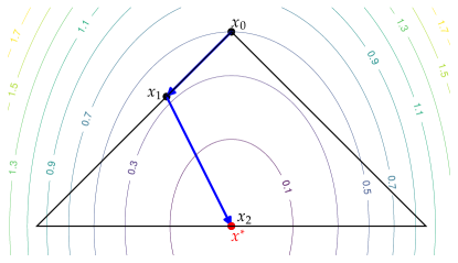
Figure 10: The Fully-Corrective Frank–Wolfe algorithm (Algorithm 3) optimizing $f(x,y)=2x^{2}+y^{2}$ over the triangle $P=\operatorname{conv}(\{(-1,0),(1,0),(0,1)\})$ with starting vertex is $x_{0}=(0,1)$. The optimum is $x^{*}=(0,0)$. As the algorithm completely minimizes $f$ over all previously seen vertices at every iteration, in this simple example the algorithm reaches the optimum after just two iterations, having seen all vertices. For comparison, the performance of the vanilla Frank–Wolfe algorithm (Algorithm 1) and the Away-step Frank–Wolfe algorithm (Algorithm 2) minimizing the same function over the same feasible region can be seen in Figures 6 and 8, respectively.

The algorithm has appeared first in [126] without proof of linear convergence. The name fully-corrective stems from the full minimization over the convex hull of the current active set and the first rigorous proof of linear convergence, to the best of our knowledge, is due to [147], via comparison to the Away-Step Frank–Wolfe algorithm (Algorithm 2), as outlined below. Moreover, note that at least with an exact linear minimization oracle, the algorithm converges in finitely many steps, as the optimum $x^{*}$ will be necessarily in the convex hull of the vertices returned by the linear minimization oracle at some point.

Theorem 2.34.

Suppose $P$ is a polytope and $f$ is $L$-smooth and $\mu$-strongly convex over $P$. Then the Fully-Corrective Frank–Wolfe algorithm (Algorithm 3) satisfies

$$f(x_{t})-f(x^{*})\leq\left(1-\min\left\{\frac{1}{2},\frac{\mu\delta^{2}}{LD^{2}}\right\}\right)^{t-1}\frac{LD^{2}}{2}$$ (92)

for all $t\geq 1$, where $D$ and $\delta$ are the diameter and the pyramidal width of the polytope $P$. In other words, the algorithm finds a solution of primal gap at most $\varepsilon>0$ after at most the following number of linear minimizations, gradient computations and convex optimizations over convex hull of some sets:

$$1+\max\left\{2,\frac{LD^{2}}{\mu\delta^{2}}\right\}\ln\left(\frac{LD^{2}}{2\varepsilon}\right)$$ (93)

The bound follows similarly to that of Theorems 2.29 or 3.2, and therefore the proof is omitted. The main observation is that every iteration makes as much progress as AFW would with a single Frank–Wolfe step and any number of immediately following away steps, and hence there are no iterations (drop steps) where the algorithm does not make provably exponential progress.

3 Improvements and generalizations of Frank–Wolfe algorithms

In the following, we will present several advanced variants of Frank–Wolfe algorithms that go beyond the basic ones, offering significant performance improvements in specific situations. We start with the easily presented and important ones in Section 8. Further, less important or more complex variants will be presented in Section 9. Algorithms, which use underlying ideas of conditional gradients, but significantly differ from the basic conditional gradient template will be relegated to Section 13.

8 Advanced variants

In this section, we present the simplest improvements to Frank–Wolfe algorithms. While usually geared towards special cases, e.g., strongly convex functions, these variants often (empirically) perform very well in other settings. Nonetheless, their worst-case convergence rates reduce to those of the vanilla Frank–Wolfe algorithm.

8.1 Pairwise Frank–Wolfe algorithm: a natural improvement of Away-step Frank–Wolfe algorithm

In the Away-step Frank–Wolfe algorithm (Algorithm 2) mentioned before, we either take an away-step or a Frank–Wolfe step. Another natural approach is to combine the two steps, performing a so-called pairwise step, which will lead us to the Pairwise Frank–Wolfe algorithm (PFW) (Algorithm 1). The Pairwise Frank–Wolfe algorithm, introduced in [147] and drawing inspiration from [173] and [182], also requires the explicit maintenance of iterates as convex combinations of active atoms. The underlying idea is to move weight in the convex decomposition $x_{t}=\sumop\slimits@_{v\in\mathcal{S}_{t}}\lambda_{v,t}v$ directly from a bad active atom to an atom provided by the linear optimization oracle. (For brevity we have omitted the explicit update rules in Line 7 of Algorithm 1, which are similar in spirit to Algorithm 2.) In contrast to this, the Away-Step Frank–Wolfe algorithm spreads the weight of this bad atom uniformly among all remaining active atoms, before adding weight to a potentially new atom in the following iteration.

Example 3.1 (PFW convergence).

The performance of the Pairwise Frank–Wolfe algorithm with line search, for the right triangle $P=\operatorname{conv}(\{(-1,0),(1,0),(0,1)\})$, is illustrated in Figure 11 for $f(x,y)=2x^{2}+y^{2}$ with optimum at $x^{*}=(0,0)$ and start vertex at $x_{0}=(0,1)$.

Figure 11: The Pairwise Frank–Wolfe algorithm (Algorithm 1) moves only along directions determined by two vertices in contrast to, e.g., the vanilla Frank–Wolfe algorithm where the direction is towards a vertex, and hence also involves the current iterate. In the small example here this allows only a limited number of directions, which is clearly visible in the trajectory. The feasible region is the triangle $P=\operatorname{conv}(\{(-1,0),(1,0),(0,1)\})$, the objective function is $f(x,y)=2x^{2}+y^{2}$. The starting vertex is $x_{0}=(0,1)$, with following iterates $x_{1},x_{2},\dots$ and the optimum is $x^{*}=(0,0)$. For comparison, the performance of the vanilla Frank–Wolfe algorithm (Algorithm 1), the Away-step Frank–Wolfe algorithm (Algorithm 2) and the Fully-Corrective Frank–Wolfe algorithm (Algorithm 3) minimizing the same function over the same feasible region can be seen in Figures 6, 8 and 10 respectively.

Algorithm 1 Pairwise Frank–Wolfe (PFW) [147]

0   Start atom $x_{0}\in P$

0   Iterates $x_{1},\dotsc\in P$

1   $\mathcal{S}_{0}\leftarrow\{x_{0}\}$, $\lambda_{x_{0},0}\leftarrow 1$

2   for $t=0$ to … do

3      $v_{t}^{\text{FW}}\leftarrow\operatorname*{argmin}_{v\in P}\mathinner{{}\langle\nabla f(x_{t}),v\rangle}$

4       $v_{t}^{\text{A}}\leftarrow\operatorname*{argmax}_{v\in\mathcal{S}_{t}}\mathinner{{}\langle\nabla f(x_{t}),v\rangle}$

5      $\gamma_{t}\leftarrow\min\left\{\frac{\mathinner{{}\langle\nabla f(x_{t}),v_{t}^{\text{A}}-v_{t}^{\text{FW}}\rangle}}{L\mathinner{{}\lVert v_{t}^{\text{A}}-v_{t}^{\text{FW}}\rVert}^{2}},\lambda_{v_{t}^{\text{A}},t}\right\}$

6       $x_{t+1}\leftarrow x_{t}+\gamma_{t}(v_{t}^{\text{FW}}-v_{t}^{\text{A}})$ {pairwise step}

7       Find convex decomposition $x_{t+1}=\sumop\slimits@_{v\in\mathcal{S}_{t+1}}\lambda_{v,t+1}v$ with $\mathcal{S}_{t+1}\subseteq\mathcal{S}_{t}\cup\{v_{t}^{\text{FW}}\}$.

8   end for

Theorem 3.2.

Suppose $P$ is a polytope and $f$ is $L$-smooth and $\mu$-strongly convex over $P$. Then the Pairwise Frank–Wolfe algorithm (Algorithm 1) satisfies

$$f(x_{t})-f(x^{*})\leq\left(1-\min\left\{\frac{1}{2},\frac{\mu\delta^{2}}{LD^{2}}\right\}\right)^{(t-1)/(3\lvert\operatorname{Vert}(P)\rvert!+1)}\frac{LD^{2}}{2}$$ (94)

for all $t\geq 0$, where $D$ and $\delta$ are the diameter and the pyramidal width of the polytope $P$, respectively. Therefore the primal gap is at most $\varepsilon$ after at most the following number of gradient computations and linear optimizations:

$$1+\bigl{(}3\lvert\operatorname{Vert}(P)\rvert!+1\bigr{)}\cdot\max\left\{2,\frac{LD^{2}}{\mu\delta^{2}}\right\}\cdot\ln\frac{LD^{2}}{2\varepsilon}.$$ (95)

The proof is similar to that of Theorem 2.29 for the Away-step Frank–Wolfe algorithm and is therefore omitted here. We only mention that beside drop steps, there is no proof for linear improvement also for so-called swap steps, where one replaces the away vertex with the Frank–Wolfe vertex, leaving all other coefficients of the active vertices unchanged. The term $3\lvert\operatorname{Vert}(P)\rvert!$ arises as a conservative bound on the number of consecutive drop steps and swap steps, similar to the factor $2$ in the proof of the Away-step Frank–Wolfe algorithm. To eliminate the large constant, one might use modified versions of the algorithm like the one in [218], using the same gradient across successive swap steps (see Algorithm 2 in the next section). In order to get a better understanding of the relative performance of FW, AFW, PFW, and FCFW, it is helpful to consider a computational example.

Example 3.3 (Performance of the FW, AFW, FCFW and PFW algorithms).

Consider minimizing an $L$-smooth and $\mu$-strongly convex function $f(x)=\frac{1}{2}\mathinner{{}\lVert Mx\rVert}_{2}^{2}+\mathinner{{}\langle b,x\rangle}$ such that $L/\mu\approx 10^{6}$ over the probability␣simplex ₁₀₀. The matrix $M$ and the vector $b$ are generated by choosing the entries uniformly at random between $0$ and $1$. By solving the optimization problem to high accuracy we find that the resulting value of $x^{*}$ for this problem is a convex combination of $10$ vertices of the polytope. Figure 12 shows the evolution of the primal gap for the different algorithms in the number of iterations with both axes in a logarithmic scale.

Figure 12: Primal gap convergence for the vanilla Frank–Wolfe algorithm (FW, Algorithm 1), the Away-step Frank–Wolfe algorithm (AFW, Algorithm 2), the Fully-Corrective Frank–Wolfe algorithm (FCFW, Algorithm 3) and the Pairwise Frank–Wolfe algorithm (PFW, Algorithm 1) in number of iterations and wall-clock time for minimizing a strongly convex and smooth quadratic function over the $99$-dimensional probability simplex using line search. The optimum is a convex combination of $10$ vertices of the polytope, explaining FCFW reaching the optimum in a small number of (possibly costly) iterations. Note the linear convergence of AFW and PFW, in contrast to the sublinear convergence of FW.

The use of the AFW, PFW, and FCFW algorithms brings a clear advantage in convergence for this class of functions over the FW algorithm. Note however that the AFW and PFW algorithms require that we maintain and update the active set $\mathcal{S}$ (this can become expensive if the size of the active set gets larger), the FCFW algorithm, on the other hand requires solving the subproblem in Line 5 of Algorithm 3 at each iteration, which can be as computationally expensive as the original problem we are trying to solve. Lastly, note that as the optimum is not contained in the interior of $\mathcal{X}$, we cannot expect the FW algorithm to have linear convergence in primal gap (as we have seen in Section 7.2), whereas the AFW, FCFW, and PFW algorithms do.

Improving Pairwise Frank–Wolfe via the Sufficient Slope Condition

Some conditional gradient variants (e.g., AFW, PFW, and also BoostFW as introduced in Section 9.1 a little later) might suffer from steps for which we cannot guarantee sufficient primal progress within the convergence analysis; these steps are usually referred to as bad steps. For example in the case of the Away-step Frank–Wolfe Algorithm and the Pairwise Frank–Wolfe Algorithm we have no primal progress guarantee for drop steps and swap steps. Usually convergence analyses ignore these bad steps, provided they ensure at least non-negative (but possibly $0$) primal progress and then argue that they cannot happen “too often”, so that in “most” steps we make enough progress.

In this section we present an adaptation of a general enhancement via the Sufficient Slope Condition (SSC) for first-order methods due to [218]. The basic idea of using SSC is to chain together bad steps without recomputing the gradient until the SSC is met; we make this precise below. One might want to think of SSC as a generalization of the scaling inequality, see e.g., Lemma 2.26. As [218] do not provide explicit convergence rates, it is not obvious how to compare the convergence rate of the enhancement with the original methods. Nevertheless, as we shall see, in the specific case of the Pairwise Frank–Wolfe Algorithm the convergence rate improves to essentially that of the Away-step Frank–Wolfe Algorithm, as the SSC enhancement eliminates the very loose theoretical bound on the number of swap steps; for the expert, the key here is that the Frank–Wolfe vertex remains the same for consecutive swap steps. For the Away-step Frank–Wolfe Algorithm we are not aware of an improved bound for the SSC-enhanced algorithm, neither are we for, e.g., the boosted FW algorithm from Section 9.1. As such, for the sake of exposition, we simplify the presentation of the SSC enhancement from [218] by specializing it to the Pairwise Frank–Wolfe Algorithm only, however in a form suggestive of how the SSC enhancement would work for the arbitrary first-order methods. More recently, it has been shown in [249] that a simple modification of the Pairwise Frank–Wolfe Algorithm is sufficient to remove swap steps by incorporating ideas from the Blended Conditional Gradient Algorithm (see Section 9.2) leading to an algorithm with improved convergence and sparsity compared to the Pairwise Frank–Wolfe Algorithm.

The main idea of SSC can be summarized as follows: In a given iteration either we made enough primal progress so that it is warranted to compute a new gradient etc or we made little to no primal progress, which (under the respective assumptions) implies that we also did not move far from the last iterate, so that we can reuse the gradient and compute a new step. As tiny steps remain close to the previous iterate, the gradient should not change much, so by reusing the previous gradient one exchanges a gradient computation for a sufficiently small error. A gradient is reused until we moved far enough from the iterate from where we computed the same gradient; then we have also made enough primal progress even if it has been achieved with a myriad of tiny steps. The important feature of this modification is that it provides good convergence rate in the number of gradient computations. However, for an overall convergence rate in the number of steps we also have to bound the number of tiny steps taken as well, which we do here for the Pairwise Frank–Wolfe variant with SSC but remains challenging in other scenarios.

The algorithm is presented in Algorithm 2. Intuitively, the pairwise direction $d_{t,i}$ is the opposite direction where the Pairwise Frank–Wolfe Algorithm would go to from the point $y_{t,i}$ provided the objective function has gradient $\nabla f(x_{t})$ there. The maximal step size $\gamma_{t,i}$ is the maximum of step sizes the algorithm would choose for any objective function and only depends on the active set. More precisely this means that, the pairwise direction is $d_{t,i}=v^{\text{A}}-v^{\text{FW}}$ where $v^{\text{A}}$ and $v^{\text{FW}}$ are the away vertex and Frank–Wolfe vertex at $y_{t,i}$ but using the gradient $\nabla f(x_{t})$ at $x_{t}$ instead of $y_{t,i}$. The maximal pairwise step size $\gamma_{t,i,\max}$ is the coefficient of the away vertex $v^{\text{A}}$ in the convex decomposition of $y_{t,i}$ into vertices of the polytope $P$. This convex combination should be maintained as in the original Pairwise Frank–Wolfe Algorithm (Algorithm 1) or the Away-step Frank–Wolfe Algorithm (Algorithm 2) and is not repeated here. The convex set _t,i is a small ball around $x_{t}$ of the points not far away from $x_{t}$ where the last gradient is reused. The original algorithm uses only the last iterate for the radius of the ball $\mathinner{{}\lVert x_{t}-z\rVert}\leq\mathinner{{}\langle\nabla f(x_{t}),d_{t,i}\rangle}\mathbin{/}(L\mathinner{{}\lVert d_{t,i}\rVert})$ and cuts it off with another restriction $\mathinner{{}\langle\nabla f(x_{t}),x_{t}-z\rangle}\geq L\mathinner{{}\lVert x_{t}-z\rVert}^{2}$. To streamline the presentation we have decreased the radius of the ball instead so that the last inequality is implied. This simplification also makes computing the step size bound $\alpha_{t,i}$ less expensive. This change is the only difference to the original algorithm in [218].

Algorithm 2 Pairwise Frank–Wolfe with SSC [218]

0   Start atom $x_{0}\in P$

0   Iterates $x_{1},\dotsc\in P$

1   for $t=0$ to … do {SSC method}

2      $y_{t,0}\leftarrow x_{t}$

3      for $i=0$ to … do

4          $d_{t,i}\leftarrow$ pairwise direction at $y_{t,i}$ for $\nabla f(x_{t})$

5         $\gamma_{t,i,\max}\leftarrow$ maximal pairwise step size

6         ${}_{t,i}\leftarrow\{z\in P\mid\mathinner{{}\lVert x_{t}-z\rVert}\leq\min_{0\leq j\leq i}\mathinner{{}\langle\nabla f(x_{t}),d_{t,i}\rangle}\mathbin{/}(L\mathinner{{}\lVert d_{t,i}\rVert})\}$

7         if $y_{t,i}\notin{}_{t,i}$ or $d_{t,i}=0$ then

8            $x_{t+1}\leftarrow y_{t,i}$

9            break

10         else

11             $\alpha_{t,i}\leftarrow\max\{\gamma:\gamma>0,\ y_{t,i}-\gamma d_{t,i}\in{}_{t,i}\}$

12            $\gamma_{t,i}\leftarrow\min\left\{\gamma_{t,i,\max},\alpha_{t.i}\right\}$

13            $y_{t,i+1}\leftarrow y_{t,i}-\gamma_{t,i}d_{t,i}$

14            if $\gamma_{t,i,\max}\geq\alpha_{t,i}$ then

15               $x_{t+1}\leftarrow y_{t,i+1}$

16               break

17            end if

18         end if

19      end for

20   end for

Note that in Line 4 the Frank–Wolfe vertex remains the same and only the away vertex changes via the inner iterations. Moreover, the additional step size bound $\alpha_{t,i}$ in Line 11 in Algorithm 2 is hard to compute for some norms like $\ell_{p}$-norms in general (easy however for $p=1,2,\infty$). Regardless, it is easy to verify that, as $y_{t,0}=x_{t}$, the first iteration of the inner loop makes exactly a pairwise step with the short step rule, since $\alpha_{t,0}=\mathinner{{}\langle\nabla f(x_{t}),d_{t,0}\rangle}/(L\mathinner{{}\lVert d_{t,0}\rVert}^{2})$. In particular, the algorithm deviates from the standard Pairwise Frank–Wolfe Algorithm only where theoretical guarantee for primal progress is insufficient, i.e., after a swap step, replacing a sequence of swap and drop steps with a sequence of a more efficient variant of drop steps.

Theorem 3.4.

Let $f$ be a $\mu$-strongly convex, $L$-smooth function over a polytope $P$ with diameter $D$ and pyramidal width $\delta$. Then for every outer iteration $t\geq 1$ of the Pairwise Frank–Wolfe Algorithm with SSC (Algorithm 2) we have:

$$h_{t}\leq\left(\frac{1}{1+\frac{\mu}{L}\cdot\frac{\delta^{2}}{(\delta+D)^{2}}}\right)^{t-1}\cdot\frac{LD^{2}}{2}.$$ (96)

Thus the primal gap is at most $\varepsilon$ after at most the following number of gradient computations and linear optimizations and at most twice as many inner iterations, or more precisely, step size limit computations (i.e., computations of the $\alpha_{t,i}$):

$$1+\left(1+\frac{L}{\mu}\cdot\frac{2D^{2}+\delta^{2}}{\delta^{2}}\right)\cdot\ln\frac{LD^{2}}{2\varepsilon}.$$ (97)

The proof largely follows [161]. The only major deviation here is the use of primal gap as progress measure instead of distance of iterates, as customary for conditional gradient algorithms. We start with a series of lemmas showing increasingly more progress in function value. Recall that $x_{t+1}=y_{t,i}$ for the largest $i$ for which the algorithm generates $y_{t,i}$.

Lemma 3.5 (Monotonicity).

The iterates of Algorithm 2 are monotonically decreasing in function value: $f(y_{t,i})\geq f(y_{t,i+1})$ for all outer iteration $t$ and inner iteration $i$. In particular, $f(y_{t,i})\geq f(x_{t+1})$.

Proof.

Using $L$-Lipschitz continuity of gradients and $y_{t,i+1}\in{}_{t,i}$ we obtain

$$\mathinner{{}\langle\nabla f(y_{t,i+1}),d_{t,i}\rangle}\geq\mathinner{{}\langle\nabla f(x_{t}),d_{t,i}\rangle}-L\mathinner{{}\lVert x_{t}-y_{t,i+1}\rVert}\cdot\mathinner{{}\lVert d_{t,i}\rVert}\geq 0.$$ (98)

Therefore

$$f(y_{t,i})-f(y_{t,i+1})\geq\mathinner{{}\langle\nabla f(y_{t,i+1}),y_{t,i}-y_{t,i+1}\rangle}=\gamma_{t,i}\mathinner{{}\langle\nabla f(y_{t,i+1}),d_{t,i}\rangle}\geq 0.\qed$$

For progress compared to the start of an inner loop, we show more progress than just monotonicity. Note that the bound also holds even for the last $y_{t,i}$ even though there might not be an inner iteration $i$.

Lemma 3.6 (Progress).

For every outer iteration $t$ and all $i$ for which $y_{t,i}$ is defined we have the following lower bound on primal and dual progress:

$$f(x_{t})-f(y_{t,i}) \geq\frac{\mathinner{{}\langle\nabla f(x_{t}),x_{t}-y_{t,i}\rangle}}{2}\geq\frac{L\mathinner{{}\lVert x_{t}-y_{t,i}\rVert}^{2}}{2},$$ (99)

$$\mathinner{{}\langle\nabla f(x_{t}),x_{t}-y_{t,i}\rangle} \geq\mathinner{{}\lVert x_{t}-y_{t,i}\rVert}\cdot\min_{0\leq j<i}\frac{\mathinner{{}\langle\nabla f(x_{t}),d_{t,j}\rangle}}{\mathinner{{}\lVert d_{t,j}\rVert}}.$$ (100)

Proof.

The core of the proof is showing Equation (100), using $x_{t}=y_{t,0}$ and $y_{t,j}-y_{t,j+1}=\gamma_{t,j}d_{t,j}$.

$$\begin{split}\mathinner{{}\langle\nabla f(x_{t}),x_{t}-y_{t,i}\rangle}&=\mathinner{{}\left\langle\nabla f(x_{t}),\sumop\slimits@_{j=0}^{i-1}\gamma_{t,j}d_{t,j}\right\rangle}=\sumop\slimits@_{j=0}^{i-1}\gamma_{t,j}\mathinner{{}\langle\nabla f(x_{t}),d_{t,j}\rangle}\\ &\geq\sumop\slimits@_{j=0}^{i}\gamma_{t,j}\mathinner{{}\lVert d_{t,j}\rVert}\cdot\min_{0\leq j<i}\frac{\mathinner{{}\langle\nabla f(x_{t}),d_{t,j}\rangle}}{\mathinner{{}\lVert d_{t,j}\rVert}}\\ &\geq\mathinner{{}\left\lVert\sumop\slimits@_{j=0}^{i-1}\gamma_{t,j}d_{t,j}\right\rVert}\cdot\min_{0\leq j<i}\frac{\mathinner{{}\langle\nabla f(x_{t}),d_{t,j}\rangle}}{\mathinner{{}\lVert d_{t,j}\rVert}}\\ &=\mathinner{{}\lVert x_{t}-y_{t,i}\rVert}\cdot\min_{0\leq j<i}\frac{\mathinner{{}\langle\nabla f(x_{t}),d_{t,j}\rangle}}{\mathinner{{}\lVert d_{t,j}\rVert}}.\end{split}$$ (101)

Using $\mathinner{{}\lVert x_{t}-y_{t,i}\rVert}\leq\min_{0\leq j<i}\mathinner{{}\langle\nabla f(x_{t}),d_{t,j}\rangle}\mathbin{/}(L\mathinner{{}\lVert d_{t,j}\rVert})$ also ensured by the algorithm, we obtain

$$\mathinner{{}\langle\nabla f(x_{t}),x_{t}-y_{t,i}\rangle}\geq\mathinner{{}\lVert x_{t}-y_{t,i}\rVert}\cdot\min_{0\leq j<i}\frac{\mathinner{{}\langle\nabla f(x_{t}),d_{t,j}\rangle}}{\mathinner{{}\lVert d_{t,j}\rVert}}\geq L\mathinner{{}\lVert x_{t}-y_{t,i}\rVert}^{2}.$$ (102)

Together with $L$-smoothness of $f$ we conclude

$$\begin{split}f(x_{t})-f(y_{t,i})&\geq\mathinner{{}\langle\nabla f(x_{t}),x_{t}-y_{t,i}\rangle}-\frac{L\mathinner{{}\lVert x_{t}-y_{t,i}\rVert}^{2}}{2}\\ &\geq\frac{\mathinner{{}\langle\nabla f(x_{t}),x_{t}-y_{t,i}\rangle}}{2}\\ &\geq\frac{L\mathinner{{}\lVert x_{t}-y_{t,i}\rVert}^{2}}{2}.\qed\end{split}$$ (103)

Now we combine these to estimate the total progress over a single inner loop.

Lemma 3.7 (Main estimation).

For every outer iteration $t$ if the inner loop terminates, there is an inner iteration $i$ satisfying either $x_{t+1}=\operatorname*{argmin}_{z\in P}\mathinner{{}\langle\nabla f(x_{t}),z\rangle}$ or

$$f(x_{t})-f(x_{t+1})\geq\frac{\mathinner{{}\langle\nabla f(x_{t}),d_{t,i}\rangle}^{2}}{2L\mathinner{{}\lVert d_{t,i}\rVert}^{2}}.$$ (104)

Proof.

For a fixed outer iteration $t$, let $i$ be the inner iteration during which the inner loop terminates. There are several cases depending on how the termination occurs.

If $d_{t,i}=0$ then $x_{t+1}=y_{t,i}=\operatorname*{argmin}_{z\in P}\mathinner{{}\langle\nabla f(x_{t}),z\rangle}$, and the lemma clearly follows.

For the other cases we first show that $\mathinner{{}\lVert x_{t}-x_{t+1}\rVert}\geq\mathinner{{}\langle\nabla f(x_{t}),d_{t,j}\rangle}\mathbin{/}(L\mathinner{{}\lVert d_{t,j}\rVert})$ for some $0\leq j\leq i$. If $y_{t,i}\notin{}_{t,i}$ then $x_{t+1}=y_{t,i}$ and $\mathinner{{}\lVert x_{t}-x_{t+1}\rVert}=\mathinner{{}\lVert x_{t}-y_{t,i}\rVert}\geq\mathinner{{}\langle\nabla f(x_{t}),d_{t,i}\rangle}\mathbin{/}(L\mathinner{{}\lVert d_{t,i}\rVert})$, and the claim follows with $j\stackrel{{\scriptstyle\textnormal{\scriptsize def}}}{{=}}i$. If $\alpha_{t,i}\leq\gamma_{t,i,\max}$ then $\gamma_{t,i}=\alpha_{t,i}$ and $x_{t+1}=y_{t,i+1}$ lies on the boundary of _t,i, i.e., $\mathinner{{}\lVert x_{t}-x_{t+1}\rVert}=\min_{0\leq j\leq i}\mathinner{{}\langle\nabla f(x_{t}),d_{t,j}\rangle}\mathbin{/}(L\mathinner{{}\lVert d_{t,j}\rVert})$, showing the claim.

Thus in all cases $\mathinner{{}\lVert x_{t}-x_{t+1}\rVert}\geq\mathinner{{}\langle\nabla f(x_{t}),d_{t,j}\rangle}\mathbin{/}(L\mathinner{{}\lVert d_{t,j}\rVert})$ for some $j$, hence by Lemma 3.6

$$f(x_{t})-f(x_{t+1})\geq\frac{L\mathinner{{}\lVert x_{t}-x_{t+1}\rVert}^{2}}{2}\geq\frac{\mathinner{{}\langle\nabla f(x_{t}),d_{t,j}\rangle}^{2}}{2L\mathinner{{}\lVert d_{t,j}\rVert}^{2}}.\qed$$

Finally, we combine these estimates with ideas of the Pairwise Frank–Wolfe Algorithm, like the scaling inequality (Lemma 2.26), to obtain a directly interpretable progress estimate, i.e., using only parameters independent of the algorithm.

Proof of Theorem 3.4.

First we show that at any point in the algorithm, the total number of inner iterations is at most twice the total number of outer iterations, counting also the iterations in progress. To this end we investigate the number of active vertices, i.e., the vertices of $P$ appearing in the convex decomposition of $y_{t,i}$.

During an outer iteration $t$, there is at most one new active vertex (the Frank–Wolfe vertex for $\nabla f(x_{t})$), while every inner iteration $i$ except the last one removes an active vertex (the away vertex) by the choice of the step size $\gamma_{t,i}=\gamma_{t,i,\max}$ as the maximal pairwise step size. Denoting by $N$ the total number of inner iterations (counting the ones from past outer iterations) up to some point in outer iteration $t$, the number of active vertices is at most $1+t-(N-t)$. As there is always at least one active vertex, we have $1+t-(N-t)\geq 1$, i.e., $N\leq 2t$ as claimed.

Now let $t$ be a fixed outer iteration. We shall show the following, from which the claimed convergence rate follows. The initial bound $h_{1}\leq LD^{2}/2$ follows from the very first iteration being identical to that of the Pairwise Frank–Wolfe Algorithm (Theorem 3.2), as mentioned above just before Theorem 3.4, hence $f(x_{1})-f(x^{*})\leq f(y_{0,1})-f(x^{*})\leq LD^{2}/2$.

We will establish the following contraction for the outer iterations:

$$h_{t+1}\leq\frac{1}{1+\frac{\mu}{L}\cdot\frac{\delta^{2}}{(\delta+D)^{2}}}\cdot h_{t}.$$ (105)

By the above, the inner loop terminates in some iteration $i$. We apply Lemma 3.7. If $x_{t+1}=\operatorname*{argmin}_{z\in P}\mathinner{{}\langle\nabla f(x_{t}),z\rangle}$ then by Lemma 3.6

$$f(x_{t})-f(x_{t+1})\geq\frac{\mathinner{{}\langle\nabla f(x_{t}),x_{t}-x_{t+1}\rangle}}{2}\geq\frac{\mathinner{{}\langle\nabla f(x_{t}),x_{t}-x^{*}\rangle}}{2}\geq\frac{h_{t}}{2},$$ (106)

i.e., $h_{t+1}\leq h_{t}/2$, and Equation (105) follows via $\mu\leq L$.

Otherwise $f(x_{t})-f(x_{t+1})\geq\frac{\mathinner{{}\langle\nabla f(x_{t}),d_{t,i}\rangle}^{2}}{2L\mathinner{{}\lVert d_{t,i}\rVert}^{2}}$ for some inner iteration $i$. Using the scaling inequality (Lemma 2.26), $L$-Lipschitz continuous gradients (via $L$-smoothness, see Lemma 1.7) and strong convexity (Lemma 2.13) we obtain

$$\begin{split}\mathinner{{}\langle\nabla f(x_{t}),d_{t,i}\rangle}&\geq\delta\frac{\mathinner{{}\langle\nabla f(x_{t}),y_{t,i}-x^{*}\rangle}}{\mathinner{{}\lVert y_{t,i}-x^{*}\rVert}}\\ &\geq\delta\frac{\mathinner{{}\langle\nabla f(y_{t,i}),y_{t,i}-x^{*}\rangle}}{\mathinner{{}\lVert y_{t,i}-x^{*}\rVert}}-L\delta\mathinner{{}\lVert x_{t}-y_{t,i}\rVert}\\ &\geq\delta\sqrt{2\mu(f(y_{t,i})-f(x^{*}))}-L\delta\mathinner{{}\lVert x_{t}-y_{t,i}\rVert}.\end{split}$$ (107)

Note that the second term above is the error we incur due to reusing the gradient $\nabla f(x_{t})$ rather than recomputing $\nabla f(y_{t,i})$. By rearranging and using

$$f(x_{t})-f(x_{t+1})\geq\frac{\mathinner{{}\langle\nabla f(x_{t}),d_{t,i}\rangle}^{2}}{2L\mathinner{{}\lVert d_{t,i}\rVert}^{2}}\geq\frac{\mathinner{{}\langle\nabla f(x_{t}),d_{t,i}\rangle}^{2}}{2LD^{2}}$$

(as $\mathinner{{}\lVert d_{t,i}\rVert}\leq D$) and Equation (99) from Lemma 3.6, together with monoticity $f(y_{t,i})\geq f(x_{t+1})$ (Lemma 3.5) we obtain

$$\begin{split}\delta\sqrt{2\mu\cdot\bigl{(}f(x_{t+1})-f(x^{*})\bigr{)}}&\leq\delta\sqrt{2\mu\cdot\bigl{(}f(y_{t,i})-f(x^{*})\bigr{)}}\\ &\leq L\delta\mathinner{{}\lVert x_{t}-y_{t,i}\rVert}+\mathinner{{}\langle\nabla f(x_{t}),d_{t,i}\rangle}\\ &\leq\delta\sqrt{2L\bigl{(}f(x_{t})-f(y_{t,i})\bigr{)}}+D\sqrt{2L\bigl{(}f(x_{t})-f(x_{t+1})\bigr{)}}\\ &\leq(\delta+D)\sqrt{2L\bigl{(}f(x_{t})-f(x_{t+1})\bigr{)}}.\end{split}$$ (108)

Hence Equation (105) follows. ∎

Decomposition-Invariant Conditional Gradient algorithm

Recall that the Away-Step and Pairwise Frank–Wolfe algorithms maintain an explicit convex decomposition of iterates, which is sometimes a disadvantage as it might introduce a significant computational overhead. To avoid the decomposition, [108] and in follow-up work [20] proposed searching for the away vertex in the minimal face $\mathcal{F}_{\mathcal{X}}(x)$ containing the current iterate $x_{t}$. More precisely, rather than solving the away-step linear optimization problem over $\operatorname{conv}(\mathcal{S})$, where $\mathcal{S}$ is the maintained active set of $x_{t}$, it is solved over $\mathcal{F}_{\mathcal{X}}(x)$; see Line 3 of Algorithm 3. The so-obtained away vertex can be easily shown to be an away vertex for some active set; this is where the term decomposition-invariant stems from. This class of algorithms usually requires two additional oracles: an away-step oracle solving the optimization problem over $\mathcal{F}_{\mathcal{X}}(x)$ and a line-search oracle providing the maximum step size for away-vertices to remain feasible as we do not have an active set anymore where we can read-off the weight of the away vertex. In other words, the main difficulty is ensuring that away steps and pairwise steps remain in the feasible region, while still making significant progress, as the convex decomposition is no longer available to compute a maximal step size. No general solution is known to this difficulty. One approach is doing line search, but it requires feasibility testing, which is not completely trivial for some polytopes.

We will follow the approach of [108] here, restricting ourselves to the important class of simplex-like integral polytopes and special step sizes, in order to help us maintain feasibility. The result is the Decomposition-invariant Pairwise Conditional Gradient algorithm of [108] presented in Algorithm 3 [20, using the form proposed by], and a similar Decomposition-invariant Away-step Frank–Wolfe algorithm of [20] (which we omit). A simplex-like polytope $\mathcal{X}$ has the following form

$$\mathcal{X}=\{x\in\mathbb{R}^{n}\mid x\geq 0,Ax=b\}$$

with only $0/1$-vertices, i.e., every coordinate of a vertex is either $0$ or $1$. The experts note that this does not cover all polytopes by projection as we require the vertices being in $\{0,1\}$. A few important examples are the probability simplex, the Birkhoff polytope (see Example 3.9) and the bipartite matching polytope. We briefly recall the argument ensuring feasibility of the iterates. Step sizes $\gamma_{t}$ are chosen to be non-increasing and of the form $2^{-k}$ for some natural number $k$, so that the coordinates of the iterate $x_{t}$ are integral multiples of $\gamma_{t}$. In particular, via an easy induction, the non-zero coordinates of $x_{t}$ are at least $\gamma_{t}$. As all vertices are $0/1$-vectors, we have

$$x_{t+1}=x_{t}+\gamma_{t}\bigl{(}v_{t}^{\text{FW}}-v_{t}^{\text{A}}\bigr{)}\geq 0,$$

noting that for coordinates $x_{t,i}=0$ we have $v_{t,i}^{\text{A}}=0$ as $v_{t}^{\text{A}}$ lies on the minimal face containing $x_{t}$ by construction. This argument explicitly uses the condition $x\geq 0$ in the definition of simplex-like polytope $\mathcal{X}$.

A novel and important feature of Algorithm 3 is that the linear convergence rate it achieves for smooth and strongly convex functions depends on the number of non-zero coordinates of the optimal solution $x^{*}$ (see Theorem 3.8) instead of the pyramidal width. Thus the convergence bound is better for sparse optima, which likely occurs only when the simplex like presentation $\mathcal{X}$ define a natural constrain set, like for the examples mentioned above.

To loop back to what we have seen before, sparsity is actually an upper bound on a local variant of pyramidal width, replacing the pyramidal width in the scaling inequality (75), namely, by [108, Lemma 2 ]:

$$\mathinner{{}\langle\psi,v^{\text{A}}-v^{\text{FW}}\rangle}\geq\frac{1}{\sqrt{\mathinner{{}\lVert y\rVert}_{0}}}\cdot\frac{\mathinner{{}\langle\psi,x-y\rangle}}{\mathinner{{}\lVert x-y\rVert}_{2}},$$ (109)

where $\mathinner{{}\lVert y\rVert}_{0}$ denotes the number of non-zero coordinates of $y$. (Note that if $y=0$ then $\mathcal{X}=\{0\}$. We exclude this trivial case to avoid dividing by zero.) We remark that sparsity as treated here is not symmetric under coordinate-flips, i.e., under transformations $x_{i}\mapsto 1-x_{i}$. It is an open question whether the sparsity notion can be improved to, e.g., the number of fractional variables.

Algorithm 3 Decomposition-invariant Pairwise Frank–Wolfe (DI-PFW) [108, 20]

0   Vertex $x_{0}$ of $\mathcal{X}$, a sequence of step sizes $\gamma_{t}$ for $t\geq 1$ with $1/\gamma_{1}$ and $\gamma_{t}/\gamma_{t+1}$ being integers for $t\geq 1$

0   Iterates $x_{1},\dotsc\in\mathcal{X}$

1   for $t=0$ to … do

2      $v_{t}^{\text{FW}}\leftarrow\operatorname*{argmin}_{v\in\mathcal{X}}\mathinner{{}\langle\nabla f(x_{t}),v\rangle}$

3      $v_{t}^{\text{A}}\leftarrow\operatorname*{argmax}_{v\in\mathcal{F}_{\mathcal{X}}(x_{t})}\mathinner{{}\langle\nabla f(x_{t}),v\rangle}$ {$\mathcal{F}_{\mathcal{X}}(x)$ is the minimal face containing $x$.}

4      $x_{t+1}\leftarrow x_{t}+\gamma_{t}(v_{t}^{\text{FW}}-v_{t}^{\text{A}})$

5   end for

We recall the convergence rate from [108, Theorem 1 ].

Theorem 3.8.

Let $f$ be a $\mu$-strongly convex, $L$-smooth convex function in the Euclidean norm over a simplex-like polytope $\mathcal{X}$. Let $\mathinner{{}\lVert x^{*}\rVert}_{0}$ denote the number of non-zero elements of $x^{*}$. Running the Decomposition-Invariant PFW algorithm 3 with step sizes

$$\gamma_{t}=\max_{k=0,1,\dotsc}\left\{2^{-k}\,\middle|\,2^{-k}\leq\sqrt{\frac{\mu}{16LD^{2}\cdot\mathinner{{}\lVert x^{*}\rVert}_{0}}}\left(1-\frac{\mu}{16LD^{2}\cdot\mathinner{{}\lVert x^{*}\rVert}_{0}}\right)^{\frac{t-1}{2}}\right\},$$ (110)

with $\mathinner{{}\lVert x\rVert}_{0}$ denoting the number of non-zero coordinates of $x$, the primal gap satisfies for all $t\geq 1$:

$$f(x_{t})-f(x^{*})\leq\frac{LD^{2}}{2}\exp\left(-\frac{\mu}{8LD^{2}\mathinner{{}\lVert x^{*}\rVert}_{0}}t\right).$$ (111)

Equivalently, the primal gap is at most $\varepsilon$ with at most the following number of linear minimizations (including minimizations over minimal faces $\mathcal{F}_{\mathcal{X}}(x_{t})$):

$$\frac{8LD^{2}\mathinner{{}\lVert x^{*}\rVert}_{0}}{\mu}\ln\frac{LD^{2}}{2\varepsilon}.$$ (112)

This algorithm is mostly beneficial for problems with a small simplex-like representation and it requires the knowledge of $L$, $\mu$, and $D$ as well as the sparsity of the optimal solution $\mathinner{{}\lVert x^{*}\rVert}_{0}$ in order to compute the step sizes. While knowing $L$, $\mu$, and $D$ can be realistic in some cases, the knowledge of the sparsity is more problematic. A good estimate of sparsity is crucial though to realize convergence in sparsity as the algorithm effectively provides guarantees in this estimate only and not the true parameter. In many important cases one can get around these parameter-estimation issues by substituting the step size rule for a line search. Nonetheless, for more general problems we face several challenges. For problems with large simplex-like representation, as is the case for the (non-bipartite) matching polytope [222] and its approximations [37] needing an exponential number of extra coordinates, sparsity is hard to interpret for the original problem, and the simplex-like representation is impractical for solving the LP subproblems. Computing the away vertex has the same challenges as computing the in-face directions for the In-Face Extended Frank–Wolfe algorithm (Algorithm 20), as we will see later on. In addition, as the vertices are assumed to be integral, often the away-step optimization problem becomes an integer program. Then we run into a complexity-theoretic issue: linear optimization problems with integrality constraints tend to be NP-hard. As such, unless co-NP is equal to NP (which is generally believed to be not the case), the away step oracle cannot be implemented as we will not have concise access to the describing constraints required to confine the optimization to the face of the current iterate (see [77] for a discussion of this problem).

One the other hand, if we have a problem that has a favorable structure – and there are many important ones, e.g., in machine learning – then the performance of DI-PFW can be quite remarkable and usually making it the fastest conditional gradient algorithms for this problem class. This is not surprising: we essentially have an algorithm with per-iteration convergence higher than that of PFW and we do not have to maintain an active set. It remains an open question whether one can find a conditional gradient algorithm without active set that circumvents these issues and still guarantees linear convergence for sharp or strongly convex functions.

Example 3.9 (A numerical run of the PFW and DI-PFW algorithms).

In Figure 13 we compare the primal gap evolution of the pairwise-step FW (PFW) and the Decomposition-invariant pairwise Conditional Gradient (DI-PFW) algorithm when both algorithms are run using line search, so that there is no need to estimate sparsity $\mathinner{{}\lVert x^{*}\rVert}_{0}$. The feasible region $\mathcal{X}$ is the Birkhoff␣polytope in $\mathbb{R}^{n\times n}$, the set of doubly stochastic matrices, i.e., nonnegative matrices, where for each row and column the entries sum up to $1$. Here however it will be convenient to disregard the matrix structure, therefore we treat every matrix in $\mathbb{R}^{n\times n}$ as a vector of its entries, i.e., an element of $\mathbb{R}^{n^{2}}$. The objective function is a quadratic $f(x)=\frac{1}{2}\mathinner{{}\lVert Qx\rVert}_{2}^{2}+\mathinner{{}\langle b,x\rangle}$ where $Q\in\mathbb{R}^{n^{2}\times n^{2}}$ and $b\in\mathbb{R}^{n^{2}}$ with $n=70$. The entries of $Q$ and $b$ are selected uniformly at random from the interval between $0$ and $1$. This results in an objective function with $L\approx 10^{6}$ and $\mu\approx 10^{-5}$. Note that for simplex-like polytopes with $0/1$ vertices, computing the away vertex in the DI-PFW algorithm, that is, solving the linear optimization problem in Line 3 of Algorithm 3 has the same computational cost as solving the linear optimization problem in Line 2, which is solved over $\mathcal{X}$ and has complexity $n^{3}$ using the Hungarian algorithm (see [68] for an overview). More concretely, and following from [108], Line 3 of Algorithm 3 is computed as:

$$v_{t}^{\text{A}}\stackrel{{\scriptstyle\textnormal{\scriptsize def}}}{{=}}\operatorname*{argmax}_{v\in\mathcal{X}}\mathinner{{}\langle d(x_{t}),v\rangle},$$

where $d(x_{t})\in\mathbb{R}^{n^{2}}$ is defined as

$$[d(x)]_{i}\stackrel{{\scriptstyle\textnormal{\scriptsize def}}}{{=}}\begin{cases}[\nabla f(x_{t})]_{i}&\text{if \ }[x_{t}]_{i}>0\\ -\infty&\text{if \ }[x_{t}]_{i}=0,\end{cases}$$

for $0\leq i\leq n^{2}$. When considering the PFW algorithm, we compute the away vertex using an active set, and loop through the vertices in $\mathcal{S}_{t}$ to find the vertex that has greatest inner product with the gradient. This has a complexity of $\mathcal{O}(\lvert\mathcal{S}_{t}\rvert n^{2})$, where $\lvert\mathcal{S}_{t}\rvert$ is the cardinality of the active set $\mathcal{S}_{t}$. This means that finding the direction towards which PFW moves has complexity $\mathcal{O}(n^{3}+\lvert\mathcal{S}_{t}\rvert n^{2})$, and finding the direction towards which DI-PFW moves has complexity $\mathcal{O}(n^{3})$, so if $n<\lvert\mathcal{S}_{t}\rvert$, we can expect the cost per iteration of the DI-PFW to be lower than that of the PFW algorithm, which would widen the difference between the primal gap convergence in wall-clock time of the two algorithms.

Figure 13: Primal gap evolution of the Pairwise Frank–Wolfe algorithm (PFW, Algorithm 1) and the Decomposition-invariant Pairwise Frank–Wolfe algorithm (DI-PFW, Algorithm 3) for a random quadratic function in dimension $4900$ over the Birkhoff polytope (i.e., doubly stochastic matrices), see Example 3.9. Note that these are log-log plots and we can clearly see that the convergence of DI-PFW is not just faster in time due to not having to maintain an explicit active set at each iteration but also in iterations due to the use of better away-vertices, not being confined to an arbitrary active set but considering all possible active sets.

For this specific instance, we can see from Figure 13 that the DI-PFW algorithm provides an advantage in both the number of iterations and wall-clock time over the PFW algorithm. The advantage is explained by DI-PFW potentially using better away-vertices, searching them from a possibly larger set. For this instance the optimum is very likely sparse as the high accuracy solution we have computed is sparse with $\mathinner{{}\lVert x^{*}\rVert}_{0}=205$. More generally, we will see also in later comparisons that the DI-PFW algorithm will have a computational advantage in wall-clock time over the PFW algorithm when solving the linear minimization problem in Line 3 of Algorithm 3 is computationally cheaper than the looping through the active set that the PFW algorithm typically performs to find an away vertex.

8.2 Adaptive step size control for conditional gradient algorithms

Recall that to avoid the cost of performing a line search, the short step rule is typically employed, which has the disadvantage of requiring a good upper bound $L$ on the smoothness of the objective function. [198] instead proposed an adaptive step size strategy (Algorithm 4) where the initial smoothness estimate is continuously adjusted as new data becomes available, creating a step size algorithm that is a blend of a backtracking line search strategy and the short step rule. The overhead from this adaptive strategy is relatively low compared to running a line search in each iteration and simply requires having access to the objective function value (often termed a zeroth-order oracle call), so that it can be often used as the go-to step size strategy.

The adaptive step size strategy of [198] has a tendency to progressively decrease the smoothness constant estimate to potentially take advantage of a locally possibly smoother behavior, and then backtracks to ensure the smoothness inequality holds; as smoothness induces primal progress, it is referred to as the sufficient decrease condition in the paper. The progressive tightening and backtracking is controlled by two parameters: the tightening parameter $\eta$ and the backtracking parameter $\tau$. In a nutshell, the adaptive step size strategy maintains an estimate $\mathaccent 0{\symlargesymbols}065{L}$ of the smoothness parameter, then performs a short step with that estimate $\mathaccent 0{\symlargesymbols}065{L}$ and verifies that the smoothness inequality is satisfied. If so, the step is accepted, otherwise $\mathaccent 0{\symlargesymbols}065{L}$ is updated and the procedure is repeated.

In conditional gradient algorithms, like the vanilla Frank–Wolfe algorithm, the Away-step Frank–Wolfe algorithm, and Pairwise Frank–Wolfe algorithm (Algorithms 1, 2, and 1), the adaptive step size strategy provides convergence rates that are essentially identical (up to constants) to the short step rule, however requiring additionally a constant number of function evaluations per iteration depending on $\eta$ and $\tau$ in the worst case. A theoretical model to leverage the progressive behavior in order to obtain strictly better rates is an open question. In particular, there is little guidance on the choice of $\tau$ and $\eta$. However, [198] claims the values $\tau=2$ and $\eta=0.9$ perform well in practice; the same values have been also used as default values in the FrankWolfe.jl Julia package [28] with very good results.

Algorithm 4 Adaptive step size strategy ($\operatorname{Ada}_{f}(x,v;\mathaccent 0{\symlargesymbols}065{L}))$ [198]

0   Objective function $f$, smoothness estimate $\mathaccent 0{\symlargesymbols}065{L}$, feasible points $x$, $v$ with $\mathinner{{}\langle\nabla f(x),x-v\rangle}\geq 0$, progress parameters $\eta\leq 1<\tau$

0   Updated estimate $\mathaccent 0{\symlargesymbols}065{L}^{*}$, step size $\gamma$

1   $M\leftarrow\eta\mathaccent 0{\symlargesymbols}065{L}$

2   loop

3      $\gamma\leftarrow\min\{\mathinner{{}\langle\nabla f(x),x-v\rangle}\mathbin{/}(M\mathinner{{}\lVert x-v\rVert}^{2}),1\}$ {compute short step for $M$}

4      if $f(x+\gamma(v-x))-f(x)\leq\gamma\mathinner{{}\langle\nabla f(x),v-x\rangle}+\frac{\gamma^{2}M}{2}\mathinner{{}\lVert x-v\rVert}^{2}$ then

5         $\mathaccent 0{\symlargesymbols}065{L}^{*}\leftarrow M$

6         return  $\mathaccent 0{\symlargesymbols}065{L}^{*}$, $\gamma$

7      end if

8      $M\leftarrow\tau M$

9   end loop

In our presentation of the adaptive step size strategy (Algorithm 4), the previous smoothness estimate $\mathaccent 0{\symlargesymbols}065{L}$ is provided as an input to the algorithm, which is then continuously updated until the smoothness condition is ensured between the current point, and the new point the algorithm intends to move towards. For simplicity, the update direction is represented by the furthest point $v$ the algorithm is willing to go in that direction. We present a modification of the vanilla Frank–Wolfe algorithm endowed with the adaptive step size strategy in Algorithm 5 as an example; all algorithms can be modified similarly by simply replacing the short step rule with this strategy. In order to choose the initial Lipschitz estimate $L_{-1}$ in Algorithm 5 or in any adaptive variant, one can simply guess (as the strategy is going to fix it anyway), e.g., via the heuristic suggested in [198]: $L_{-1}\stackrel{{\scriptstyle\textnormal{\scriptsize def}}}{{=}}\mathinner{{}\lVert\nabla f(x_{0})-\nabla f(x_{0}+\gamma(v_{0}-x_{0}))\rVert}/(\gamma\mathinner{{}\lVert v_{0}-x_{0}\rVert})$, where $\gamma>0$ is a small constant, and $v_{0}=\operatorname*{argmin}_{x\in\mathcal{X}}\mathinner{{}\langle\nabla f(x_{0}),x\rangle}$. The original work [198] claims the value $\gamma=0.001$ working well in practice, which we empirically confirmed too.

Algorithm 5 Adaptive vanilla Frank–Wolfe (AdaFW) [198]

  As Algorithm 1, but choosing an initial $L_{-1}$ and replacing Line 3 with

  $L_{t},\gamma_{t}\leftarrow\operatorname{Ada}_{f}(x_{t},v_{t};L_{t-1})$

Example 3.10 (A numerical example).

In Figure 14 (left) we compare the primal gap evolution of the vanilla Frank–Wolfe algorithm (Frank–Wolfe), and the Pairwise Frank–Wolfe algorithm (PFW), and their variants with the adaptive step size strategy (denoted by the ‘Ada’ prefix in the graphs) via Algorithm 4. The feasible region is the unit $\ell_{1}$-ball and the objective function is a quadratic $f(x)=\frac{1}{2}\mathinner{{}\lVert Qx\rVert}_{2}^{2}+\mathinner{{}\langle b,x\rangle}$ where $Q\in\mathbb{R}^{n\times n}$ and $b\in\mathbb{R}^{n}$ with $n=200$. The entries of $Q$ and $b$ are selected uniformly random from the interval between $0$ and $1$. This results in an objective function with $L\approx 10043$ and $\mu\approx 0.0005$. Figure 14 (right) shows the evolution of the smoothness estimate $\mathaccent 0{\symlargesymbols}065{L}$ used by the adaptive algorithms. All adaptive variants use $\tau=2$, $\eta=0.9$ and a starting smoothness estimate of $0.01$. Note that the smoothness estimate used by the adaptive variants hovers around $150$, and is much smaller than the $L$-smoothness parameter of the function, which results in larger step sizes and greater progress.

Figure 14: Performance in primal gap for Frank–Wolfe algorithms with and without adaptive step size rules (left figure) minimizing a strongly convex and smooth quadratic function over the $200$-dimensional unit $\ell_{1}$-ball, see Example 3.10 for details. The algorithms that use the adaptive step size rule (Algorithm 4) have the prefix “Ada”, the remaining algorithms simply use the short step rule. The algorithms depicted are the vanilla Frank–Wolfe algorithm (FW, Algorithm 1), and the Pairwise Frank–Wolfe algorithm (PFW, Algorithm 1). The right figure shows the evolution of the local smoothness estimate $\mathaccent 0{\symlargesymbols}065{L}$ used for adaptive step size. Note that we have used hollow markers to differentiate between the line plots that overlap. Note how this estimate is much smaller than the smoothness constant $L\approx 10000$, leading to faster convergence for the adaptive variants.

In fact the adaptive step size strategy has two more properties that make it extremely powerful.

Remark 3.11 (Adaptivity to local smoothness).

One significant advantage in comparison to the short step rule is that the adaptive step size strategy can adapt to local smoothness depending on the trajectory of the algorithm. This can be observed in the example above, where the estimated smoothness constant is much smaller then the worst-case smoothness ($L\approx 10000$). The result is a significantly improved real-world performance.

Remark 3.12 (Multiplicative vs. additive accuracy).

The second advantage of the adaptive step size strategy in comparison to line searches is that in actual computations we rarely perform a line search but rather an approximate one or a backtracking line search with finite precision. Once the function change is below that additive threshold, a line-search based algorithm cannot further progress, so that high-precision solutions can often not be obtained. In contrast, the adaptive step size strategy estimates the local smoothness and errors in the estimation of $L$ lead to a multiplicative error (rather than an additive error) in progress, so that the optimal solution can still be approached, just a little slower.

Remark 3.13 (Implementation notes for Algorithm 4).

In practice, the test in Line 4 of Algorithm 4 sometimes fail due to numerical inaccuracy, leading to rapid increase of the smoothness estimate $M$. As a consequence the resulting steps have length close to $0$ and optimization would stall.

As a countermeasure to numerical errors, one should relax the required progress, trading theoretical optimality of the short step estimation for error tolerance. A good way is to include a factor $\alpha\leq 1$ for the step size:

$$f(x+\gamma(v-x))-f(x)\leq\alpha\gamma\mathinner{{}\langle\nabla f(x),v-x\rangle}+\frac{\alpha^{2}\gamma^{2}M}{2}\mathinner{{}\lVert x-v\rVert}^{2}.$$ (113)

For example the FrankWolfe.jl package uses $\alpha=0.5$ as default, which works well in practice. The case $\alpha=1$ is the case without the relaxation, exactly as it appears in Algorithm 4. Note that the factor $\alpha$ is not included in the returned step size, as there are no numerical issues there.

Moreover, note that this relaxation affects the convergence speed only by a multiplicative factor of about $1/\alpha^{2}$.

8.3 Lazification

Depending on the feasible region of interest, the cost of the linear programming oracle, while still much smaller than the cost of projections, might be huge. This is for example the case if the feasible region $\mathcal{X}$ is the convex hull of solutions to a hard combinatorial optimization problem, such as the traveling salesman problem, where a single solution to the linear programming problem can easily take minutes to hours for moderately-sized instances. In such cases it is highly desirable to reduce the cost of the linear programming oracle in conditional gradient algorithms. Facing such expensive linear programming oracles, the questions are (1) do we really have to call the (expensive) LP oracle in each iteration (2) is there a way to reuse information from previous calls

The currently known weakest relaxation of an LP oracle that answers the two questions above in the affirmative while maintaining the same convergence rates (up to constant factors) as the more expensive LP oracle was proposed by [40]: a Weak Separation Oracle (Oracle 6), which searches only for a solution that is good enough, i.e., one that has an objective value better than a given threshold. In particular, this oracle model is weaker than the approximate LP oracle model in [131], and even weaker than approximation with multiplicative error, as it requires a (realistic) additive improvement goal $\phi$ only rather than some approximately optimal solution. Upon presentation with an improvement goal $\phi$ and the current iterate, the weak separation oracle will either return a positive answer: an improving vertex $y$ realizing the target improvement $\phi$ over the current iterate (w.r.t. the provided linear function) within a constant multiplicative error $K$, or a negative answer that the improvement goal $\phi$ is impossible (which then also serves as an approximate optimality certificate as we will see).

Algorithm 6 Weak Separation LP Oracle for $\mathcal{X}$ (LPsep)

0   Linear objective $c$, point $x\in\mathcal{X}$, accuracy $K\geq 1$, target objective $\phi>0$

0   $\begin{cases*}y\in\mathcal{X},&with $\mathinner{{}\langle c,x-y\rangle}>\phi/K$ \quad\lx@algorithmic@hfill(positive answer)\\ \textbf{false}{},&if $\mathinner{{}\langle c,x-z\rangle}\leq\phi$ for all $z\in\mathcal{X}$ \quad\lx@algorithmic@hfill(negative answer)\end{cases*}$

The weak separation oracle model enables two important speed-ups compared to a single LP oracle call: caching and early termination. Caching searches first a small cache of vertices for an improving vertex meeting the improvement requirement, falling back to the more costly linear programming oracle in case of a cache miss. The cache is maintained by some heuristic, like recently used or previously computed vertices in a context where the oracle is used repeatedly. In conditional gradient algorithms natural implementations are (1) the list of previously computed vertices (2) the active set of vertices for those variants that maintain active sets Early termination reuses an LP oracle implementation, which typically would compute an (approximately) optimal solution going through many vertices in the process but would terminate the search early once a vertex satisfying the improvement condition is found. Another important reason to use lazification is in order to obtain much sparser solutions in the number of vertices (or atoms) used to express the iterate as a convex combination. This is promoted by reusing vertices (or atoms), via the cache whenever possible. For completeness the following remark is in order:

Remark 3.14 (Linear Optimization realizes Weak Separation).

The Weak-Separation Oracle can be realized with a single call to a Linear Optimization Oracle.

As mentioned before, replacing the linear programming oracle with the weak separation oracle in conditional gradient algorithms provides similar convergence rates (up to small constant factors) in the number of oracle calls, where the cheapness of the oracle calls to the weak separation oracle should compensate for the overhead of maintaining the cache and loss in constant factors etc.

Here we discuss only the lazified vanilla Frank–Wolfe algorithm in detail, leading to the Parameter-free Lazy Conditional Gradient algorithm (Algorithm 7), as well as showing how the same approach carries over to other conditional gradient algorithm variants exemplified with the Away-Step Frank–Wolfe algorithm. The choice of $\phi_{0}$ affects the convergence rate mainly in the initial part of the algorithm: a choice that is too large choice leads to many initial negative oracle answers, while a choice that is too small can lead to slow progress in the initial iterations, due to unnecessarily weak improving directions. The condition $\phi_{0}\geq h_{0}/2$ is included in the algorithm only to simplify the convergence proof by omitting inefficient initial iterations. While this condition is not directly verifiable in practice as $h_{0}$ might not be known, the original paper ensured it via setting $\phi_{0}=\min_{x}\mathinner{{}\langle\nabla f(x_{0}),x-x_{0}\rangle}\mathbin{/}2$, i.e., to be half of the Frank–Wolfe gap, requiring a single, initial linear programming oracle call.

Algorithm 7 Parameter-free Lazy Conditional Gradient (LCG) [40]

0   Start atom $x_{0}\in\mathcal{X}$, accuracy $K\geq 1$, initial goal $\phi_{0}>0$

0   Iterates $x_{1},\dotsc\in\mathcal{X}$

1   for $t=0$ to … do

2      $v_{t}\leftarrow\text{LPsep}_{\mathcal{X}}(\nabla f(x_{t}),x_{t},\phi_{t},K)$

3      if $v_{t}=\textbf{false}{}$ then

4         $x_{t+1}\leftarrow x_{t}$

5         $\phi_{t+1}\leftarrow\phi_{t}/2$

6      else

7         $\gamma_{t}\leftarrow\operatorname*{argmin}_{0\leq\gamma\leq 1}f(x_{t}+\gamma(v_{t}-x_{t}))$ or adaptive step size strategy (Algorithm 4)

8         $x_{t+1}\leftarrow x_{t}+\gamma_{t}(v_{t}-x_{t})$

9         $\phi_{t+1}\leftarrow\phi_{t}$

10      end if

11   end for

The $\phi_{t}$ are the thresholds to be used in the Weak Separation Oracle, which are intended to be kept within a constant factor of the Frank–Wolfe gap $g_{t}$ to ensure progress comparable to the (non-lazy) vanilla Frank–Wolfe algorithm. A negative answer certifies that $\phi_{t}\geq g_{t}\geq h_{t}$, so that the controlled decrease of $\phi_{t}$ by any constant factor between $0$ and $1$ (the choice of $1/2$ is arbitrary) ensures we remain within a fixed constant factor of the Frank–Wolfe gap and at the same time we keep $\phi_{t}$ large to find descent directions with sufficient progress via the Weak Separation Oracle.

Theorem 3.15.

For an $L$-smooth convex objective function $f$ over a convex domain $\mathcal{X}$ with diameter $D$, if $h_{0}/2\leq\phi_{0}\leq LD^{2}/2$ then Algorithm 7 achieves primal gap at most $\varepsilon$, i.e., $f(x_{t})-f(x^{*})\leq\varepsilon$ in at most $\mathcal{O}(K^{2}LD^{2}/\varepsilon)$, or more precisely the following number of gradient computations and weak separation oracle calls:

$$\max\left\{\left\lceil\log_{2}\frac{\phi_{0}}{\varepsilon}\right\rceil,0\right\}+\left\lceil\frac{8K^{2}LD^{2}}{\varepsilon}\right\rceil.$$ (114)

Note that up to a constant factor the last term $\mathcal{O}(LD^{2}/\varepsilon)$ is the rate for the vanilla Frank–Wolfe algorithm (Theorem 2.2). The first term $\log(\phi_{0}/\varepsilon)$ is the number of negative oracle calls, until $\phi_{t}$ drops below $\varepsilon$, upon which the next negative oracle answer ensures $h_{t}\leq\varepsilon$.

The condition $h_{0}/2\leq\phi_{0}\leq LD^{2}/2$ is satisfiable by two linear oracle calls without knowledge of parameters like $L$ or $D$, similar to Remark 2.4: With the cost of at most one linear oracle call find an arbitrary $x_{-1}\in\mathcal{X}$. Then choose $x_{0}\stackrel{{\scriptstyle\textnormal{\scriptsize def}}}{{=}}\operatorname*{argmin}_{x\in\mathcal{X}}\mathinner{{}\langle\nabla f(x_{-1}),x\rangle}$ and $\phi_{0}\stackrel{{\scriptstyle\textnormal{\scriptsize def}}}{{=}}g(x_{0})\mathbin{/}2$ and clearly $h_{0}/2\leq g(x_{0})$. Now, note that for any $y\in\mathcal{X}$, one has $\mathinner{{}\langle\nabla f(x_{-1}),x_{0}\rangle}\leq\mathinner{{}\langle\nabla f(x_{-1}),y\rangle}$ by the choice of $x_{0}$. Rearranging and using $L$-Lipschitzness of gradients lead to

$$\begin{split}\mathinner{{}\langle\nabla f(x_{0}),x_{0}-y\rangle}&\leq\mathinner{{}\langle\nabla f(x_{0})-\nabla f(x_{-1}),x_{0}-y\rangle}\\ &\leq\mathinner{{}\lVert\nabla f(x_{0})-\nabla f(x_{-1})\rVert}_{*}\cdot\mathinner{{}\lVert x_{0}-y\rVert}\\ &\leq L\mathinner{{}\lVert x_{0}-x_{-1}\rVert}\cdot\mathinner{{}\lVert x_{0}-y\rVert}\leq LD^{2}.\end{split}$$

Thus $g(x_{0})\leq LD^{2}$ justifying the choice of $\phi_{0}$ above. However, even for an arbitrary choice of $\phi_{0}$ and $x_{0}$ the algorithm converges with a similar rate (even if $h_{0}>LD^{2}$) at the cost of a longer initial burn-in phase; in the case that ${}_{0}>LD^{2}/2$ is chosen too large we have linear convergence (at least) until ${}_{t}\leq LD^{2}/2$.

Proof.

First note that the primal gap $h_{t}$ is obviously non-increasing. The main claim is that $\phi_{t}\geq h_{t}/2$ for every iteration $t$, which we prove by induction on $t$. For $t=0$ this holds by assumption. In an iteration $t$ when the weak separation oracle returns a negative answer, this guarantees $\phi_{t}\geq g_{t}$ and hence $\phi_{t}\geq h_{t}$. In the next iteration, we will have $\phi_{t+1}=\phi_{t}/2\geq h_{t}/2=h_{t+1}/2$. The remaining case is an iteration $t$ with a positive oracle answer, where $\phi_{t}\geq h_{t}/2$ by assumption. Then simply $\phi_{t+1}=\phi_{t}\geq h_{t}/2\geq h_{t+1}/2$.

The above argument also shows that right after $\lceil\log_{2}(\phi_{0}/\varepsilon)\rceil$ many negative oracle answer, we have $h_{t}\leq\phi_{t}\leq\varepsilon$. This upper bounds the number of negative oracle answers until reaching $h_{t}\leq\varepsilon$. (Actually, this upper bound only holds if $\phi_{0}>\varepsilon$, otherwise we have $h_{t}\leq\varepsilon$ after a single negative oracle answer.)

It remains to estimate the number of iterations with positive oracle calls, which we do by estimating the primal progress during these iterations. When the oracle returns a positive answer in iteration $t$, using Lemma 1.5 we have the following per iteration progress (estimating line search using the short step rule), which is the same as used several times before:

$$h_{t}-h_{t+1}\geq\frac{\phi_{t}}{2K}\min\left\{1,\frac{\phi_{t}}{KLD^{2}}\right\}=\frac{\phi_{t}^{2}}{2K^{2}LD^{2}}\geq\frac{h_{t}^{2}}{8K^{2}LD^{2}}.$$ (115)

Here we have used $\phi_{t}\geq h_{t}/2$. Thus after $k$ positive oracle in the final phase it holds $h_{t}\leq 8KLD^{2}/(k+8)$, as can be easily shown by induction using $h_{0}\leq LD^{2}$.

Summing up the positive and negative oracles answers provides the claimed upper bounds. ∎

Lazification applies also to other conditional gradient algorithms, such as, e.g., the Away-step Frank–Wolfe algorithm (Algorithm 2), which we demonstrate below for the sake of completeness. Making the search for both the away vertex and the Frank–Wolfe vertex lazy yields the Lazy Away-step Frank–Wolfe algorithm (Algorithm 8), where Line 3 contains the weakened, lazy search. Here the cache is essentially provided by the active set that is maintained. The other parts of the algorithm are essentially the same, so we have again omitted the details of the update of the active set for readability. In practice, one has to go through the whole active set anyway in search of the away vertex, hence searching for both, an away vertex and a Frank–Wolfe vertex to implement lazification comes at no extra cost, and the fallback to a slower algorithm if no suitable vertex has been found is the same as before; we make this strategy more precise in Remark 3.17 for the important case where the lazification wraps the LP oracle.

Algorithm 8 Lazy Away-step Frank–Wolfe (Lazy AFW) [40]

0   Start atom $x_{0}\in P$, accuracy $K\geq 1$, initial goal $\phi_{0}\geq h_{0}/2$ {E.g., $\phi_{0}\stackrel{{\scriptstyle\textnormal{\scriptsize def}}}{{=}}\max_{x\in\mathcal{X}}\mathinner{{}\langle\nabla f(x_{0}),x_{0}-x\rangle}\mathbin{/}2$}

0   Iterates $x_{1},\dotsc\in P$

1   $\mathcal{S}_{0}\leftarrow\{x_{0}\}$, $\lambda_{x_{0},0}\leftarrow 1$

2   for $t=0$ to … do

3       Find $v_{t}\in\mathcal{S}_{t}$ with $\mathinner{{}\langle\nabla f(x_{t}),v_{t}-x_{t}\rangle}\geq\phi_{t}/K$ or $v_{t}\in P$ with $\mathinner{{}\langle\nabla f(x_{t}),x_{t}-v_{t}\rangle}\geq\phi_{t}/K$ unless $\mathinner{{}\langle\nabla f(x_{t}),v-x_{t}\rangle}\leq\phi_{t}$ for all $v\in\mathcal{S}_{t}$ and $\mathinner{{}\langle\nabla f(x_{t}),x_{t}-v\rangle}\leq\phi_{t}$ for all $v\in P$.

4      if $v_{t}$ found then

5         if $\mathinner{{}\langle\nabla f(x_{t}),v_{t}-x_{t}\rangle}\geq\phi_{t}/K$ and $v_{t}\in\mathcal{S}_{t}$ then {away step}

6            $d_{t}=x_{t}-v_{t}$, $\gamma_{\max}=\frac{\lambda_{v_{t},t}}{1-\lambda_{v_{t},t}}$

7         else {Frank–Wolfe step}

8            $d_{t}=v_{t}-x_{t}$, $\gamma_{\max}=1$

9         end if

10         $\gamma_{t}\leftarrow\min\left\{\frac{\mathinner{{}\langle\nabla f(x_{t}),d_{t}\rangle}}{L\mathinner{{}\lVert d_{t}\rVert}^{2}},\gamma_{\max}\right\}$ or adaptive step size strategy (Algorithm 4)

11         $x_{t+1}\leftarrow x_{t}-\gamma_{t}d_{t}$

12         $\phi_{t+1}\leftarrow\phi_{t}$

13         Find convex combination of $x_{t+1}$: set $\mathcal{S}_{t+1}$ and $\lambda_{v,t+1}$ for $v\in\mathcal{S}_{t+1}$. {see Algorithm 2}

14      else {No $v_{t}$ found; update dual estimate}

15         $x_{t+1}\leftarrow x_{t}$

16         $\phi_{t+1}\leftarrow\phi_{t}/2$

17      end if

18   end for

Algorithm 8 has a similar convergence rate as the original Away-step Frank–Wolfe algorithm. However the lazification of the Away-step Frank–Wolfe algorithm significantly improves sparsity of the iterates in actual computations. We include a sketch of the convergence proof.

Theorem 3.16.

Let $f$ be an $L$-smooth and $\mu$-strongly convex function over a polytope $P$ with diameter $D$ and pyramidal width $\delta$. Then the Lazy AFW algorithm (Algorithm 8) ensures $h_{t}\leq\varepsilon$ for the primal gap after $\mathcal{O}(\log(\phi_{0}/\varepsilon)+K^{2}LD^{2}/(\mu\delta^{2})\log(h_{0}/\varepsilon))$, or more precisely the following number of gradient computations and weak separation oracle calls:

$$\max\left\{\left\lceil\log_{2}\frac{\phi_{0}}{\varepsilon}\right\rceil,0\right\}+1+2\cdot\left\lceil\frac{4K^{2}LD^{2}}{\mu\delta^{2}}\max\left\{\ln\frac{h_{0}}{\varepsilon},0\right\}\right\rceil.$$ (116)

Proof sketch.

The proof is analogous to that of Theorem 3.15, so we present only the details that differ. The main difference is in estimating the number of positive oracle answers after the first negative oracle call, reusing ideas from Theorem 2.29. For example, the number of drop steps is estimated the same way as at most half the number of steps with a positive oracle answer, adding a factor of $2$. In the remaining part of the proof we consider only non-drop steps. Via Geometric Strong Convexity (Lemma 2.27) we have $2\phi_{t}\geq\mathinner{{}\langle\nabla f(x_{t}),v^{\text{A}}-v^{\text{FW}}\rangle}\geq\sqrt{2\mu\delta^{2}\cdot h_{t}}$ in addition to $\phi_{t}\geq h_{t}/2$ after the first negative oracle call, resulting for non-drop steps in a progress bound of the form (cf., Equation (83))

$$h_{t}-h_{t+1}\geq\min\left\{\frac{\phi_{t}}{2K},\frac{\phi_{t}^{2}}{2K^{2}LD^{2}}\right\}\geq\min\left\{1,\frac{\mu\delta^{2}}{KLD^{2}}\right\}\frac{h_{t}}{4K}=\frac{\mu\delta^{2}}{4K^{2}LD^{2}}\cdot h_{t},$$ (117)

This results in an upper bound of $(4K^{2}LD^{2}/(\mu\delta^{2}))\ln(h_{0}/\varepsilon)$ iterations with a positive oracle answer, which are not drop steps, happening after the first negative oracle answer.

In conclusion, we obtain an overall bound that is similar to Theorem 3.15, with the last two terms replaced, and an extra factor of $2$ (which accounts for drop steps). ∎

The bound simplifies when $\phi_{0}$ and $x_{0}$ are chosen as in Theorem 3.15, at the additional cost of two linear minimizations.

Remark 3.17 (Typical implementation of LPSep via LMO).

Typically the weak separation oracle is realized via wrapping the LMO in a smart way. This results in a few extra possibilities for improvements as we detail now. We demonstrate this for $\text{LPsep}_{\mathcal{X}}(\nabla f(x_{t}),x_{t},\phi_{t},K)$ in Algorithm 7 but the same applies for Algorithm 8 with the only difference that we can combine the search for a lazy solution directly with the search for an away vertex. Given an LMO and a list of previously visited vertices $\mathcal{L}$ we can implement $\text{LPsep}_{\mathcal{X}}(\nabla f(x_{t}),x_{t},\phi_{t},K)$ as follows: (1) Check whether any vertex $x\in\mathcal{L}$ satisfies $\mathinner{{}\langle\nabla f(x_{t}),x_{t}-x\rangle}>\phi/K$. If so return such an $x$. (2) Otherwise call the LMO (potentially with early termination) to solve $x=\operatorname*{argmin}_{v\in\mathcal{X}}\mathinner{{}\langle\nabla f(x_{t}),v\rangle}$. If $x$ satisfies $\mathinner{{}\langle\nabla f(x_{t}),x_{t}-x\rangle}>\phi/K$ return $x$. (3) Otherwise return false and $g(x_{t})=\mathinner{{}\langle\nabla f(x_{t}),x_{t}-x\rangle}$, which is the Frank–Wolfe gap at $x_{t}$ (negative call). In most reasonable implementations one would choose $K=1$.

With this implementation, we obtain the Frank–Wolfe gap in the case of a negative call and we can use this information to more effectively update $\phi_{t}$ as $\phi_{t+1}\leftarrow\min\{\phi_{t}/2,g(x_{t})\}$. This improved update reduces unnecessary and potentially expensive LMO calls that are guaranteed to lead to negative answers and no progress: we have to scale $\phi_{t}$ down to the Frank–Wolfe gap anyways before we can obtain a positive call with actual progress again. Note that typically calls to the weak separation oracle with negative answer are much more expensive than those with positive answers: the positive one are usually obtained via the cache or an early-terminated LMO call, whereas the negative ones require an optimal solution, i.e., a full LMO call in order to ensure $\mathinner{{}\langle\nabla f(x_{t}),x_{t}-x\rangle}\leq\phi$ for all $x\in\mathcal{X}$.

Care has to be taken to keep $\mathcal{L}$ small, so that search over $\mathcal{L}$ remains cheaper than an LMO call. E.g., in the extreme case that the feasible region is a polytope $P$ and $\mathcal{L}$ is the set of all its vertices, searching over $\mathcal{L}$ is the same and hence as hard a problem as linear optimization over $P$.

We refer the interested reader to [40, 39, 38] for methodological considerations and [53, 28] for implementation related aspects.

Remark 3.18 (Trade-off lazification vs. vanilla method).

While having the same worst-case convergence rates, as the lazified algorithm does not solve the LMO subproblem exactly but only uses sufficiently good solutions, the obtained descent directions might provide less progress per iteration compared to those that would have been employed by the vanilla method. This is a consequence of the smoothness inequality and that the primal progress (using the short step rule or line search) is essentially lower bounded proportional to $\mathinner{{}\langle\nabla f(x_{t}),x_{t}-v_{t}\rangle}^{2}$. Moreover, the lazified version usually has to maintain a cache of previously visited vertices over which it has to search for sufficiently good vertices. Sometimes this comes for free as, e.g., for the lazy AFW algorithm as the active set has to be maintained anyways at other times this creates an overhead. On the other hand, the execution of the weak separation oracle can often be several orders of magnitude faster than the LMO. As such in actual computations a natural trade-off arises: less per-iteration progress vs. faster iterations in wall-clock time. In particular if the LMO is somewhat expensive, dominating the iteration cost of the algorithm, lazification usually provides excellent performance.

Example 3.19 (A numerical run of the lazy variants).

Figure 15: Primal gap evolution for minimizing a $900$-dimensional quadratic function over the spectrahedron, see Example 3.19 for details. We compare the performance of the vanilla Frank–Wolfe algorithm (FW, Algorithm 1), the Away-step Frank–Wolfe algorithm (AFW, Algorithm 2), the Lazy Conditional Gradient algorithm (LCG, Algorithm 7), and the Lazy Away-step Frank–Wolfe algorithm (Lazy AFW, Algorithm 8). Note that in spite of Lazy AFW converging slower than AFW in number of iterations (as expected), it outperforms it in wall-clock time.

In Figure 15 we compare the primal gap evolution of the vanilla Frank–Wolfe algorithm (FW) and the Away-step Frank–Wolfe (AFW) algorithm with their lazy variants (LCG and Lazy AFW). For the separation oracle in the algorithms we first search among the vertices in the active set for an appropriate vertex. If no such vertex is found, the algorithms fall back to performing a linear minimization oracle call, and checking if the conditions in Oracle 6 are satisfied. Note that this requires maintaining an active set for the LCG iterates. The feasible region used is the set of all matrices in $\mathbb{R}^{d\times d}$ of nuclear norm less than $1$, i.e., the spectrahedron, and the objective function is a quadratic $f(x)=\frac{1}{2}\mathinner{{}\lVert Qx\rVert}_{2}^{2}+\mathinner{{}\langle b,x\rangle}$ where $Q\in\mathbb{R}^{d^{2}\times d^{2}}$ and $b\in\mathbb{R}^{d^{2}}$ with $d=30$. The entries of $Q$ and $b$ are selected uniformly at random from the interval between $0$ and $1$. The images shown in Figure 15 show the evolution of the primal gap in iterations and time. Note that the results in time are implementation dependent, however they help to better understand the benefits and trade-offs of lazification. As we can see, the Lazy AFW algorithm sometimes make less primal gap progress per iteration than the AFW algorithm, however, the Lazy AFW iterations are often cheaper than the AFW iterations, which makes the Lazy AFW converge faster in wall-clock time than the AFW algorithm. The cheaper computational cost of the Lazy AFW iterations is due to the fact that the Lazy AFW algorithm combines search for an away vertex with the search for a sufficiently good vertex that guarantees enough primal progress, so that the Lazy AFW has smaller additional cost that for LCG. On the other hand, in this instance progress in iteration is essentially the same for the lazy algorithms as their non-lazy counterparts, demonstrating that the advantage of lazy variants is cheaper oracle calls compared to linear minimization.

8.4 Conditional Gradient Sliding algorithm

In this section we will use the Euclidean norm. Recall that the vanilla Frank–Wolfe algorithm requires $\mathcal{O}(1/\varepsilon)$ gradient evaluations and $\mathcal{O}(1/\varepsilon)$ linear optimizations for obtaining a primal gap at most $\varepsilon$ for convex smooth objective functions. In this section, we present the Conditional Gradient Sliding algorithm (CGS) [151], which reduces the required gradient evaluations to the minimal number (see Table 2 in Section 6.2), without increasing the number of linear optimizations. In order to achieve this, CGS (Algorithm 9) is essentially an implementation of Nesterov’s accelerated projected gradient descent algorithm [192], using the vanilla Frank–Wolfe algorithm for performing approximate projections back into the feasible regions. The key point is that the latter does not require additional gradient evaluations of the original functions: it is simply minimizing the quadratic arising from projection in Euclidean norm. The subproblems in Line 4 in Algorithm 9 provide the approximate solution (with accuracy $\eta_{t}$ in iteration $t$) to the following projection problem (note that the arguments of $\operatorname*{argmin}$ differ by a constant term $\mathinner{{}\lVert\nabla f(x_{t})\rVert}_{2}^{2}$ and a constant scaling factor $\eta_{t}/2$)

$$\operatorname*{argmin}_{x\in\mathcal{X}}\mathinner{{}\langle\nabla f(w_{t}),x\rangle}+\frac{\eta_{t}}{2}\mathinner{{}\lVert x-x_{t}\rVert}_{2}^{2}=\operatorname*{argmin}_{x\in\mathcal{X}}\mathinner{{}\left\lVert x-x_{t}+\frac{1}{\eta_{t}}\nabla f(w_{t})\right\rVert}_{2}^{2}.$$

For completeness, the simplified conditional gradient subroutine that arises is given in Algorithm 10.

Algorithm 9 Conditional Gradient Sliding (CGS) [151]

0   Start point $x_{0}\in\mathcal{X}$, step sizes $0\leq\gamma_{t}\leq 1$, learning rates $\eta_{t}>0$, accuracies $\beta_{t}\geq 0$

0   Iterates $x_{1},\dotsc\in\mathcal{X}$

1   $y_{0}\leftarrow x_{0}$

2   for $t=0$ to … do

3      $w_{t}\leftarrow(1-\gamma_{t})y_{t}+\gamma_{t}x_{t}$

4       $x_{t+1}\leftarrow\operatorname{CG}(\nabla f(w_{t}),x_{t},\eta_{t},\beta_{t})$

5      $y_{t+1}\leftarrow y_{t}+\gamma_{t}(x_{t+1}-y_{t})$

6   end for

Algorithm 10 $\text{CG}(g_{0},u_{0},\eta,\beta)$

1   for $k=0$ to … do

2      $v_{k}\leftarrow\operatorname*{argmin}_{v\in\mathcal{X}}\mathinner{{}\langle g_{k},v\rangle}$

3      if $\mathinner{{}\langle g_{k},u_{k}-v_{k}\rangle}\leq\beta$ then

4         return  $u_{k}$

5      end if

6       $\alpha_{k}\leftarrow\min\left\{\frac{\mathinner{{}\langle g_{k},u_{k}-v_{k}\rangle}}{\eta\mathinner{{}\lVert u_{k}-v_{k}\rVert}^{2}},1\right\}$ {step size according to short step rule}

7      $u_{k+1}\leftarrow u_{k}+\alpha_{k}(v_{k}-u_{k})$ {update of primal solution}

8      $g_{k+1}\leftarrow g_{0}+\eta(u_{k+1}-u_{0})$ {gradient of the projection problem}

9   end for

Theorem 3.20.

Let $\mathcal{X}$ be a compact convex set with diameter $D$ and $f\colon\mathcal{X}\to\mathbb{R}$ be an $L$-smooth convex function in the Euclidean norm. Then CGS (Algorithm 9) with $\gamma_{t}=3/(t+3)$, $\eta_{t}=3L/(t+2)$, and $\beta_{t}=LD^{2}/((t+1)(t+2))$ satisfies for all iterates $t\geq 1$,

$$f(y_{t})-f(x^{*})\leq\frac{15LD^{2}}{2(t+1)(t+2)}.$$

Equivalently, the primal gap is at most $\varepsilon$ after at most Thus, the FOO and LMO complexities are respectively: $\mathcal{O}(\sqrt{LD^{2}/\varepsilon})$ gradient computations and $\mathcal{O}(LD^{2}/\varepsilon)$ linear minimizations.

Theorem 3.20 shows that under the proposed setting of parameters, CGS achieves the optimal LMO and FOO complexity (Section 6.2). However, it is possible to improve the FOO complexity’s dependence on $D$. Below, Theorem 3.21 shows that by fixing the maximum number of iterations ahead of time, one can replace the dependence on $D$ with a dependence on the initial distance to the set of minimizers; observe the dependence of $\beta_{t}$ on $T$. In the general setting it is implicitly assumed that $T=+\infty$. This improvement, now relying on the initial distance to the minimizers, immediately allows for restart schemes as used in Section 13.2.

Theorem 3.21.

Let $\mathcal{X}$ be a compact convex set with diameter $D$ and $f\colon\mathcal{X}\to\mathbb{R}$ be an $L$-smooth convex function. Let $D_{0}\geq\max_{x^{*}\in\operatorname*{argmin}_{\mathcal{X}}f}\mathinner{{}\lVert x_{0}-x^{*}\rVert}$ and fix the maximum number of iterations $T\geq 0$. Consider CGS (Algorithm 9) with $\gamma_{t}=2/(t+2)$, $\eta_{t}=2L/(t+1)$, and $\beta_{t}=2LD_{0}^{2}/(T(t+1))$. Then

$$f(y_{T})-f(x^{*})\leq\frac{6LD_{0}^{2}}{T(T+1)}.$$

Equivalently, the primal gap is at most $\varepsilon$ after at most $\mathcal{O}(LD_{0}^{2}/\varepsilon)$ gradient computations and $\mathcal{O}(LD^{2}/\varepsilon+\sqrt{LD_{0}^{2}/\varepsilon}$ linear minimizations.

In the absence of a better estimate for $D_{0}$ in Theorem 3.21, we can always choose $D_{0}=D$. The achieved FOO and LMO complexities in Theorem 3.21 are optimal for smooth convex minimization, see Section 6.2.

See [210] for convergence rates for non-convex objective functions.

Example 3.22 (CGS performance comparison for smooth convex functions).

(a) Primal gap convergence in FOO calls

(b) Primal gap convergence in LMO calls

Figure 16: Primal gap convergence of a smooth convex function in oracle calls for the CGS algorithm (Algorithm 9) for and the vanilla FW algorithm (Algorithm 1) with three different step size strategies. The problem optimizes a smooth convex but not strongly convex function over the space of positive semidefinite matrices of unit nuclear norm. Note that for this problem, in contrast to the FW algorithms which require $\mathcal{O}(1/\varepsilon)$ calls to the FOO oracle to reach a primal gap at most $\varepsilon$, the CGS algorithm requires $\mathcal{O}(1/\sqrt{\varepsilon})$ FOO calls. The dashed pink line is the theoretical bound on FOO calls from Theorem 3.20.

In Figure 16 we compare the performance of the CGS algorithm (Algorithm 9) for smooth convex functions and the FW algorithm (Algorithm 1), in FOO and LMO calls required to reach a primal gap at most $\varepsilon$, when minimizing a smooth convex function $f$ over the space of positive semi-definite matrices of unit trace in $\mathbb R^{10\times 10}$. We run the FW algorithm with three different step size strategies, namely, the $\gamma_{t}=2/(2+t)$ step size, the short step rule, and line search. Note that the CGS algorithm, does not require exact line searches for $f$, but requires knowledge of the smoothness constant of the function and the diameter of the feasible region, or some $D_{0}\geq\max_{x^{*}\in\operatorname*{argmin}_{\mathcal{X}}f}\mathinner{{}\lVert x_{0}-x^{*}\rVert}$.

The objective function $f$ is generated by taking a random matrix $Q$ in $\mathbb R^{n\times n}$ with entries drawn uniformly between $0$ and $1$ and $n=100$, and computing the spectral decomposition of $Q^{\top}Q=\sumop\slimits@_{i=1}^{n}\lambda_{i}u_{i}u_{i}^{\top}$ with $\lambda_{1}\geq\lambda_{2}\geq\dots\geq\lambda_{n}\geq 0$. We then change the smallest eigenvalue of $Q^{\top}Q$ to zero, i.e, compute $M^{\top}M=\sumop\slimits@_{i=1}^{n-1}\lambda_{i}u_{i}u_{i}^{\top}$, which is a positive semi-definite matrix. (This equation does not determine $M$ uniquely, but it is not necessary to define the objective function, as it depends only through $M^{\top}M$ on $M$.) We also construct a vector $b$ whose entries are drawn uniformly between $0$ and $1$, and we set $f(x)=\frac{1}{2}\mathinner{{}\lVert Mx\rVert}_{2}^{2}+\mathinner{{}\langle b,x\rangle}$. The resulting objective function is $2500$-smooth and convex.

We have included the FOO oracle complexity from Theorem 3.20 as a dashed line on the left of Figure 16, to highlight the difference between the algorithms’ FOO complexities. While FOO oracle complexity of CGS is $\mathcal{O}(1/\sqrt{\varepsilon})$ for a primal gap of $\varepsilon$, that of the other algorithms shown on the image is $\mathcal{O}(1/\varepsilon)$.

CGS for strongly convex objectives

In order to also match the optimal FOO complexity when $f$ is additionally strongly convex, [151] propose the restart scheme presented in Algorithm 11, which is quite natural once one has obtained Theorem 3.21 as mentioned earlier (see, e.g., [202] for a discussion on restart schemes). It consists of iteratively running CGS for a fixed number of iterations $T$, and halving the accuracy schedule in-between. Note that $\gamma_{t}$, $\eta_{t}$, and $\beta_{t}$ denote sequences for $t=0$ to $t=T-1$.

Algorithm 11 Conditional Gradient Sliding (CGS) for strongly convex objectives [151]

0   Start point $w_{0}\in\mathcal{X}$, estimate $\phi_{0}\geq f(w_{0})-f(x^{*})$, smoothness constant $L>0$ and strong convexity constant $\mu>0$

0   Iterates $x_{1},\dotsc\in\mathcal{X}$

1   for $s=0$ to … do

2      Let $w_{s+1}$ be the last point output by the CGS algorithm (Algorithm 9) when run for $T=\left\lceil 2\sqrt{6L/\mu}\right\rceil$ iterations with parameters $x_{0}=w_{s}$, $\eta_{t}=2L/(t+1)$, $\alpha_{t}=2/(t+2)$ and $\beta_{t}=\frac{8L\phi_{0}s^{-2}}{\mu T(t+1)}$.

3   end for

Theorem 3.23.

Let $\mathcal{X}$ be a compact convex set with diameter $D>0$ and $f\colon\mathbb{R}^{n}\rightarrow\mathbb{R}$ be an $L$-smooth $\mu$-strongly convex function in the Euclidean norm. Then the CGS algorithm for strongly convex functions (Algorithm 11) satisfies for all iteration $s\geq 0$,

$$f(w_{s})-f(x^{*})\leq\frac{\phi_{0}}{2^{s}}.$$

Equivalently, the primal gap is at most $\varepsilon$ after at most $\mathcal{O}(\sqrt{L/\mu}\log(\phi_{0}/\varepsilon))$ gradient computations and $\mathcal{O}(LD^{2}/\varepsilon+\sqrt{L/\mu}\log(\phi_{0}/\varepsilon))$ linear minimizations.

While we have seen better convergence rates for special convex domains, like polytopes (Section 7.4) and strongly convex sets (Section 7.3), the theorem provides a tradeoff for arbitrary convex domains, drastically reducing the number of first-order oracle calls in exchange for extra linear minimization, compared to the vanilla Frank–Wolfe algorithm (Theorem 2.2).

Example 3.24 (CGS performance comparison for the strongly convex case).

In Figure 17 we compare the performance of the CGS algorithm (Algorithm 11) and the FW algorithm (Algorithm 1) for three different step size strategies, in FOO and LMO calls required to reach an primal gap at most $\varepsilon$, when minimizing a smooth, strongly convex function $f$ over the $500$-dimensional unit $\ell_{1}$-ball. As in Example 3.22, the step sizes strategies used for FW are the $\gamma_{t}=2/(2+t)$ step size, the short step rule, and line search.

(a) Primal gap convergence in FOO calls

(b) Primal gap convergence in LMO calls

Figure 17: Primal gap convergence for smooth strongly convex optimization in oracle calls for the CGS algorithm (Algorithm 11) and the vanilla FW algorithm (Algorithm 1) with three different step size strategies. The optimum is in the interior of the feasible region, so the FW algorithm with short step rule and line search converges linearly. The dashed pink line is the theoretical bound on FOO calls from Theorem 3.23.

The objective function is generated by generating a random orthonormal basis for $\mathbb R^{500}$, selecting a minimum eigenvalue of $\mu=1$, and a maximum eigenvalue of $L=100$, a set of $498$ remaining eigenvalues drawn uniformly between $\mu$ and $L$, and using these ingredients to build a positive definite matrix in $\mathbb R^{500}$. The unconstrained minimizer of the $f$ is placed in the interior of the unit $\ell_{1}$-ball, and so we expect to obtain linear convergence for the FW algorithm with the short step rule and line search (see Section 7.2).

As we can observe from the figure shown on the left of Figure 17, the number of FOO calls needed to reach a primal gap at most $\varepsilon$ is $\mathcal{O}(\sqrt{L/\mu}\log 1/\varepsilon)$ for the CGS algorithm for strongly convex functions, whereas the FW algorithm requires $\mathcal{O}(L/\mu\left(D/r\right)^{2}\log 1/\varepsilon)$ calls, where $r$ is the radius of the largest ball around $x^{*}$ that is contained in $\mathcal{X}$. We have added a dashed line depicting the bound on the number of FOO calls from Theorem 3.23 to aid in the comparison of the algorithms. Note that the FOO oracle complexity of the CGS algorithm has a better dependence on the condition number $L/\mu$, and does not have the dimension dependent term $D/r$. Using the AFW algorithm (Algorithm 2) with the short step rule or line search to solve this problem, we obtain very similar results to those of the FW algorithm with short step or line search, respectively, in FOO and LMO calls, but with a a higher computational cost, due to the need to maintain an active set at each iteration. Note that the FW algorithm does not converge linearly in general for this class of problems (smooth and strongly convex), while the AFW algorithm converges linearly if the feasible region is a polytope. On the other hand, the CGS algorithm (Algorithm 11) requires a linear number of FOO calls and a sublinear number of LMO calls for any compact convex feasible region.

8.5 Sharpness a.k.a. Hölder Error Bound (HEB)

Sharpness is a weakening of strong convexity, introduced in [204], leading to convergence rates between $\mathcal{O}(1/\varepsilon)$ and $\mathcal{O}(\log 1/\varepsilon)$. The weakening comes in three aspects (1) allowing a non-unique minimum to the objective function (2) generalizing the exponent $2$ (3) local to the neighborhood of the minima (only) Sharpness is also known as the Hölder(-ian) error bound [125], the sharp minima condition [205] (more generally Polyak-Łojasiewicz condition), or the strict minima condition [189]. Although it is not as well studied as strong convexity, it has been widely used to obtain faster rates than $\mathcal{O}(1/\varepsilon)$, up to linear convergence (see, e.g., [223, 262, 138, 66, 137] for recent developments). Similarly, Hölder smoothness generalizes smoothness by using a different exponent than $2$ and can be combined with sharpness to capture a wide variety of convergence regimes. Here we will confine ourselves to the standard smooth case though and we refer the reader to [138] for details and convergence results.

Sharpness basically captures how fast the functions increases around its optimal solutions. Recall that we denote by ^∗ the set of optimal solutions to $\min_{x\in\mathcal{X}}f(x)$; if the feasible region $\mathcal{X}$ is not clear from the context we write ${}_{\mathcal{X}}^{*}$.

Definition 3.25 (Sharpness a.k.a. Hölder Error Bound condition).

Let $\mathcal{X}$ be a compact convex set. A convex function $f$ is $(c,\theta)$-sharp (over $\mathcal{X}$) with $0<c<\infty$, $0<\theta\leq 1$ if for all $x\in\mathcal{X}$ and $x^{*}\in{}_{\mathcal{X}}^{*}$ we have

$$c\cdot\bigl{(}f(x)-f(x^{*})\bigr{)}^{\theta}\geq\min_{y\in{}_{\mathcal{X}}^{*}}\mathinner{{}\lVert x-y\rVert}.$$ (118)

Figure 18: Graph of $(1,\theta)$-sharp function $f(x)=\lvert x\rvert^{1/\theta}$ for various $\theta$

The restriction $\theta\leq 1$ is justified by the easy observation that a convex function cannot be $(c,\theta)$-sharp for $\theta>1$. Moreover, it is straightforward that a non-constant $L$-smooth and $(c,\theta)$-sharp function must satisfy $\theta\leq 1/2$ [189] (and $L\geq 2/c^{2}$ for $\theta=1/2$, which will be used in Corollary 3.33). Often sharpness is required only in a neighborhood of ^∗, resulting in convergence rates improving only after an initial burn-in phase, see [138, 66]. For simplicity of exposition we assume sharpness over the whole feasible region $\mathcal{X}$.

Every $\mu$-strongly convex function is clearly $(\sqrt{2/\mu},1/2)$-sharp however there are $(c,1/2)$-sharp functions which are not strongly convex, see the following example. These appear in, e.g., signal processing and machine learning, see, e.g., [104, 102] and follow-up work by these authors as well as [138, 66] and references contained therein.

Example 3.26 (Distance to a closed convex set inside the domain).

An easy example of a sharp function is distance to a non-empty closed convex set $C$

$$f_{C}(x)\stackrel{{\scriptstyle\textnormal{\scriptsize def}}}{{=}}\min_{y\in C}\mathinner{{}\lVert x-y\rVert}.$$

Obviously, ${}^{*}=C$, and $f_{C}$ is $(1,1)$-sharp over any convex set $\mathcal{X}$ containing $C$, as the defining inequality of sharpness holds with equality for all $x\in\mathbb{R}^{n}$.

We turn now to polytope domains, for which we recall a special case of the Hoffman bound from [125].

Lemma 3.27 (Hoffman bound).

Let $P$ be a polytope and $A$ a linear function on $P$ (with values in an arbitrary vector space). Then for some $c>0$ for any $x,y\in P$ one has

$$\mathinner{{}\lVert Ax-Ay\rVert}\geq c\operatorname{dist}(x,\{z\in P\mid Az=Ay\}).$$ (119)

In particular, $c$ depends only on $P$ and $A$.

This is the key to the following example.

Example 3.28 (Composition of a strongly convex function and a linear one over a polytope).

A common class of $(c,1/2)$-sharp functions consist of functions of the form $f(x)=g(Ax)$, a composition of a $\mu$-strongly convex function $g$ and a linear function $A$ over a polytope $\mathcal{X}$. This class includes functions, which have several minima and hence are not strongly convex, this is the case for non-injective $A$. In other words, these are functions like $f(x,y)=x^{2}$, which are strongly convex in some coordinates ($x$ in the example), and are independent of the rest of coordinates ($y$ in the example).

For completeness, we reproduce the verification of sharpness following [101, 23]. Besides strong convexity, we use $\nabla f(x)=A^{\top}\nabla g(Ax)$, i.e., $\mathinner{{}\langle\nabla g(Ax),Ay\rangle}=\mathinner{{}\langle\nabla f(x),y\rangle}$, and also that $\mathinner{{}\langle\nabla f(x^{*}),x-x^{*}\rangle}\leq 0$ for $x\in\mathcal{X}$ by minimality.

$$\begin{split}f(x)-f(x^{*})&=g(Ax)-g(Ax^{*})\\ &\geq\mathinner{{}\langle\nabla g(Ax^{*}),Ax-Ax^{*}\rangle}+\mu\frac{\mathinner{{}\lVert Ax-Ax^{*}\rVert}^{2}}{2}\\ &=\mathinner{{}\langle{\nabla f(x^{*})},x-x^{*}\rangle}+\mu\frac{\mathinner{{}\lVert Ax-Ax^{*}\rVert}^{2}}{2}\geq\mu\frac{\mathinner{{}\lVert Ax-Ax^{*}\rVert}^{2}}{2}.\end{split}$$ (120)

This is very close to strong convexity, the only difference is having the distance between $Ax$ and $Ax^{*}$ instead of $x$ and $x^{*}$. Nonetheless we conclude that the minimal set of $f$ is ${}^{*}=\{z\in P\mid Az=Ax^{*}\}$. Thus we continue by the Hoffman bound (Equation (120)), for some $c>0$ depending only on $f$ and $\mathcal{X}$

$$f(x)-f(x^{*})\geq\mu\frac{\mathinner{{}\lVert Ax-Ax^{*}\rVert}^{2}}{2}\geq\frac{\mu c^{2}}{2}\operatorname{dist}(x,{}^{*})^{2}.$$

Thus $f$ is $(\mu c^{2}/2,1/2)$-sharp over $\mathcal{X}$.

When the polytope $\mathcal{X}$ is bounded, there is a slight generalization with an additional linear summand: the function $f(x)=g(Ax)+\mathinner{{}\langle b,x\rangle}$ is $1/2$-sharp (with still $g$ strongly convex, $A$ linear). See [23, Lemma 2.5 ] for a proof, we only note boundedness is used to control the additional linear summand, e.g., $f(x)=\mathinner{{}\langle b,x\rangle}$ is obviously not $(c,\theta)$-sharp for $\theta<1$ over any polytope where $f$ is unbounded above.

Obviously, for any sharp function on $\mathbb{R}^{n}$, its restriction to a convex set containing ^∗, the set of all its minima in $\mathbb{R}^{n}$, is sharp with the same parameters. However, sharpness needs no longer be preserved when restricting to convex sets not containing ^∗. This makes it much harder to construct sharp functions over a bounded domain. We present examples highlighting this subtle fact, showing in particular that several assumptions in the constructions above are not superfluous.

Example 3.29 (Difficulties with sharpness over bounded domains).

As a warm-up, we consider the function commonly used for constructing local, infinitely differentiable functions: $h\colon\mathbb{R}\to\mathbb{R}$ via $h(x)=e^{-1/x^{2}}$ (extending continuously to the point $0$, i.e., $h(0)=0$). This function has a unique minimum at $0$ with value $h(0)=0$, and it is not sharp: $\lim_{x\to 0}(h(x)-h(0))^{\theta}/\lvert x\rvert=\infty$ for all $\theta>0$. However the function is convex in a neighborhood of $0$, i.e., for $-\varepsilon\leq x\leq\varepsilon$ with a suitable $\varepsilon>0$.

We use the function $h$ to construct other examples of non-sharp functions under the Euclidean norm. Consider the closed convex planar set $\smash{\mathcal{X}\stackrel{{\scriptstyle\textnormal{\scriptsize def}}}{{=}}\{(x,y)\mid-\varepsilon\leq x\leq\varepsilon},\allowbreak h(x)\leq y\leq h(\varepsilon)\}$ with the standard Euclidean norm. Consider the quadratic function $f(x,y)=y^{2}$, which is the composition of the strongly convex $1$-dimensional function $g\colon\mathbb{R}\to\mathbb{R}$ and the linear function $A\colon\mathbb{R}^{2}\to\mathbb{R}$ defined via $g(t)=t^{2}$ and $A(x,y)=y$. We show that it is not sharp over $\mathcal{X}$, a compact convex set, which is not a polytope, in contrast to Example 3.28. Restricted to $\mathcal{X}$, it clearly has a unique minimum, namely, $x=y=0$. However, $f$ is not sharp, as for all $\theta>0$ we have $\lim_{x\to 0}(f(x,h(x))-f(0,0))^{\theta}/\mathinner{{}\lVert(x,h(x))-(0,0)\rVert}_{2}=\lim_{x\to 0}h(x)^{2\theta}/\sqrt{x^{2}+h(x)^{2}}\geq\lim_{x\to 0}h(x)^{2\theta}/\lvert x\rvert=+\infty$. Similarly, the linear function $A$ is not sharp either on $\mathcal{X}$, which is the distance function to the interval $\mathcal{Y}\stackrel{{\scriptstyle\textnormal{\scriptsize def}}}{{=}}\{(x,0)\mid-\varepsilon\leq x\leq\varepsilon\}$, in contrast to Example 3.26.

A variant of this example is the distance function $d$ to $\mathcal{X}$ on $\mathcal{Y}$, which has its unique minimum also at $(0,0)$, and satisfies $d(0,0)=0\leq d(x,0)\leq\mathinner{{}\lVert(x,0)-(x,h(x))\rVert}_{2}=h(x)$ for $-\varepsilon\leq x\leq\varepsilon$, again showing that $d$ is not sharp because $h$ is not sharp. In this example the feasible region is even a polytope.

Interestingly, in the unconstrained case ($\mathcal{X}=\mathbb{R}^{n}$) a property (which is beyond the scope of the discussion here) closely related to sharpness almost always holds in finite dimensional spaces. As a consequence, any real-valued lower semicontinuous, convex, subanalytic function $f$ defined on a neighborhood $U$ of a compact convex set $\mathcal{X}$ is sharp, provided its minimum set ${}^{*}_{U}$ on $U$ is non-empty and contained in $\mathcal{X}$. The Huber loss is an example of such a function, which is an average distance to a set of points based on a smoothened version of the absolute value function, see [66]. Note that the functions in Example 3.29 violate the condition ${}^{*}_{U}\subseteq\mathcal{X}$.

Lemma 3.30 ([30]).

Let $f\colon\mathbb{R}^{n}\to\mathbb{R}\cup\{+\infty\}$ be a lower semicontinuous, convex, and subanalytic function with a global minimum. Then for any bounded set $\mathcal{K}\subset\mathbb{R}^{n}$, there exists $0<\theta<1$ and $c>0$ such that for all $x\in\mathcal{K}$,

$$\operatorname{dist}\left(x,\operatorname*{argmin}_{\mathbb{R}^{n}}f\right)\leq c\left(f(x)-\min_{\mathbb{R}^{n}}f\right)^{\theta}.$$

In general there is no easy way to estimate sharpness parameters, which are required for most gradient descent style algorithms in order to exploit sharpness. However via restarts [223, 138, see], i.e., trying out various values for sharpness parameters in a smart way, gradient descent style algorithms can be made adaptive to these parameters in order to achieve these improved convergence rates. This is unnecessary for conditional gradient algorithms as they usually do not explicitly depend on these parameters and in fact are adaptive to those parameters using line search or the short step rule [262, 138, 66, see], i.e., conditional gradient algorithms usually automatically adapt to the sharpness parameters without explicit knowledge of them.

The first-order oracle complexity for minimization of smooth, convex, $(c,\theta)$-sharp functions over closed convex sets is $\Omega(\min\{n,1/\varepsilon^{1/2-\theta}\})$ for $\theta<1/2$ and $\Omega(\min\{n,\ln(1/\varepsilon)\})$ for $\theta=1/2$, where $n$ denotes the linear dimension of the ambient space (i.e., $\mathcal{X}\subseteq\mathbb{R}^{n}$) [189]; clearly the bounds are of interest only in the so-called large-scale regime where $n$ is assumed to be very large (otherwise other methods, such as e.g., conjugate gradients may exist with complexity $\mathcal{O}(n)$). For conditional gradient algorithms [138, 66], these complexity bounds are achieved for $\theta=1/2$, and within a factor of $2$ in the exponent $1/2-\theta$ for $\theta<1/2$. Rather than reproducing these results, we will present only the key estimation enabled by sharpness, and as an illustrative example, derive sharpness-induced convergence rates for the Away-Step Frank–Wolfe algorithm (see Algorithm 2).

Lemma 3.31 (Primal gap bound from sharpness).

Let $f$ be a $(c,\theta)$-sharp convex function. Then for all $x\in\mathcal{X}$ there is an optimal point $x^{*}\in{}^{*}$ depending on $x$

$$\frac{1}{c}\bigl{(}f(x)-f(x^{*})\bigr{)}^{1-\theta}\leq\frac{\mathinner{{}\langle\nabla f(x),x-x^{*}\rangle}}{\mathinner{{}\lVert x-x^{*}\rVert}}.$$ (121)

Proof.

This simply follows from convexity and sharpness:

$$\frac{\mathinner{{}\langle\nabla f(x),x-x^{*}\rangle}}{\mathinner{{}\lVert x-x^{*}\rVert}}\geq\frac{f(x)-f(x^{*})}{c\bigl{(}f(x)-f(x^{*})\bigr{)}^{\theta}}=\frac{1}{c}\bigl{(}f(x)-f(x^{*})\bigr{)}^{1-\theta}.\qed$$

Turning to the Away-Step Frank–Wolfe algorithm, we follow the proof of Theorem 2.29. Our starting point is the following straightforward replacement of Lemma 2.27 by combining Lemma 3.31 with the scaling inequality from Lemma 2.26. Note that all other modifications work the same way: we simply combine the scaling inequality for the respective setting with Lemma 3.31.

Lemma 3.32 (Geometric sharpness).

Let $P$ be a polytope with pyramidal width $\delta>0$ and let $f$ be a $(c,\theta)$-sharp convex function over $P$. Recall from Section 7.4 the Frank–Wolfe vertex $v^{\text{FW}}=\operatorname*{argmin}_{v\in P}\mathinner{{}\langle\nabla f(x),v\rangle}$ and the away vertex $v^{\text{A}}=\operatorname*{argmax}_{v\in\mathcal{S}}\mathinner{{}\langle\nabla f(x),v\rangle}$ with $S\subseteq\operatorname{Vert}(P)$, so that $x\in\operatorname{conv}(S)$. Then

$$\frac{1}{c}\bigl{(}f(x)-f(x^{*})\bigr{)}^{1-\theta}\leq\frac{\mathinner{{}\langle\nabla f(x),v^{\text{A}}-v^{\text{FW}}\rangle}}{\delta}.$$ (122)

Proof.

The statement follows from combining Equation (75) with Lemma 3.31 for $\psi=\nabla f(x)$. We have

$$\frac{1}{c}\bigl{(}f(x)-f(x^{*})\bigr{)}^{1-\theta}\leq\frac{\mathinner{{}\langle\nabla f(x),x-x^{*}\rangle}}{\mathinner{{}\lVert x-x^{*}\rVert}}\leq\frac{\mathinner{{}\langle\nabla f(x),v^{\text{A}}-v^{\text{FW}}\rangle}}{\delta}.\qed$$

We are ready to generalize the convergence rate of Away-Step Frank–Wolfe algorithm (Algorithm 2) to sharp objective functions. As mentioned earlier, [23] proved linear convergence for functions of the form $f(x)=g(Ax)+\mathinner{{}\langle b,x\rangle}$ with $g$ strongly convex and $A$ linear).

Corollary 3.33.

Let $f$ be a $(c,\theta)$-sharp, $L$-smooth function $f$. Then the Away-Step Frank–Wolfe algorithm (Algorithm 2) has the following convergence rates in primal gap after $t$ iterations over a polytope $P$ with diameter $D$ and pyramidal width $\delta$. For $\theta<1/2$ the convergence rate is

$$h_{t} \leq\begin{cases}\frac{LD^{2}}{2^{\lceil(t-1)/2\rceil}}&1\leq t\leq t_{0},\\[4.30554pt] \frac{(c^{2}LD^{2}/\delta^{2})^{1/(1-2\theta)}}{\bigl{(}1+(1/2-\theta)\lceil(t-t_{0})/2\rceil\bigr{)}^{1/(1-2\theta)}}=\mathcal{O}\bigl{(}(2/t)^{1\mathbin{/}(1-2\theta)}\bigr{)}&t\geq t_{0},\end{cases}$$ (123)

$$\text{where }t_{0} \stackrel{{\scriptstyle\textnormal{\scriptsize def}}}{{=}}\max\left\{2\left\lfloor\log_{2}\left(\frac{LD^{2}}{\bigl{(}c^{2}LD^{2}/\delta^{2}\bigr{)}^{1\mathbin{/}(1-2\theta)}}\right)\right\rfloor+1,1\right\}.$$ (124)

For $$\theta=1/2$$ the convergence rate is

$$h_{t} \leq\left(1-\frac{\delta^{2}}{2c^{2}LD^{2}}\right)^{\lceil(t-1)/2\rceil}\frac{LD^{2}}{2}.$$ (125)

Equivalently, for a primal gap error of at most $\varepsilon>0$ the algorithm performs at most the following number of linear optimizations:

$$\begin{cases}\mathcal{O}\left(\frac{c^{2}LD^{2}}{\delta^{2}(1/2-\theta)\varepsilon^{1-2\theta}}\right)&\theta<1/2,\ \varepsilon\leq(c^{2}LD^{2}/\delta^{2})^{1/(1-2\theta)},\\[4.30554pt] 1+\frac{4c^{2}LD^{2}}{\delta^{2}}\ln\frac{LD^{2}}{2\varepsilon}&\theta=1/2.\end{cases}$$ (126)

Proof.

The proof largely follows that of Theorem 2.29, so we point out only the difference. Below the first inequality is similar to (83), but then we apply Lemma 3.32, for which recall that $d_{t}=v_{t}^{\text{FW}}-v_{t}^{\text{A}}$ is the pairwise direction.

$$\begin{split}h_{t}-h_{t+1}&\geq\min\left\{\gamma_{t,\max}\frac{\mathinner{{}\langle\nabla f(x_{t}),-d_{t}\rangle}}{2},\frac{\mathinner{{}\langle\nabla f(x_{t}),-d_{t}\rangle}^{2}}{2L\mathinner{{}\lVert d_{t}\rVert}^{2}}\right\}\\ &\geq\min\left\{\gamma_{t,\max}\frac{h_{t}}{2},\frac{\delta^{2}h_{t}^{2(1-\theta)}}{2c^{2}LD^{2}}\right\}=\min\left\{\frac{\gamma_{t,\max}}{2},\frac{\delta^{2}h_{t}^{1-2\theta}}{2c^{2}LD^{2}}\right\}\cdot h_{t}.\end{split}$$ (127)

Therefore,

$$h_{t+1}\leq\left(1-\min\left\{\frac{\gamma_{t,\max}}{2},\frac{\delta^{2}h_{t}^{1-2\theta}}{2c^{2}LD^{2}}\right\}\right)h_{t}.$$ (128)

From this the convergence rate follow by applying Lemma 2.21. The lemma is applied to the sequence $h_{t}$ with iterations resulting in drop steps omitted, so that the step inequalities hold with $\gamma_{t,\max}$ replaced by $1$. The omission of drop steps is compensated by adjustment of indices, replacing $t$ with $\lceil(t-1)/2\rceil$ in the exponents exploiting the fact that at most half of the steps can be drop steps up to any iteration $t$. For $\theta=1/2$, we additionally use $L\geq 2/c^{2}$ and $\delta\leq D$ to simplify the constant $\min\{1/2,\delta^{2}/(2c^{2}LD^{2})\}=\delta^{2}/(2c^{2}LD^{2})$ in the recursion. ∎

Remark 3.34 (Connection to gradient dominated property).

Closely related to sharpness is the gradient dominated property, a special case of which was already introduced in Definition 2.12: a function $f$ is $(c,\theta)$-gradient dominated for some $c,\theta>0$ if for all $x$ in the domain of $f$

$$\frac{1}{c}\bigl{(}f(x)-f(x^{*})\bigr{)}^{1-\theta}\leq\mathinner{{}\lVert\nabla f(x)\rVert}_{*},$$ (129)

where $x^{*}$ is the minimum place of $f$ as usual. In particular, $c$-gradient dominated is the case where $\theta=1/2$. Gradient dominance, similar to sharpness, is a local property and can be considered a natural weakening of strong convexity. As already mentioned, most convergence proofs that involve strong convexity almost immediately carry over to the gradient dominated case.

At least for smooth functions with minima lying in the relative interior of the domain, gradient dominance is equivalent to sharpness by the following lemma; see [32], which appeared online in 2015, for more on this.

Lemma 3.35 (Gradient dominated versus sharp).

Let $\mathcal{X}\subseteq\mathbb{R}^{n}$ be a compact convex set, $f\colon\mathcal{X}\to\mathbb{R}$ be a differentiable convex function, and $0<\theta<1$ be a number. If $f$ is $(c,\theta)$-sharp for some $c>0$ then it is $(c,\theta)$-gradient dominated. Conversely, if $f$ is smooth, $(c,\theta)$-gradient dominated for some $c>0$, and its set ^∗ of minima lies in the relative interior of $\mathcal{X}$, then $f$ is $(c^{\prime},\theta)$-sharp for some $c^{\prime}>0$.

Proof.

First assume $f$ is $(c,\theta)$-sharp. By Lemma 3.31, for any $x\in\mathcal{X}$ there is an $x^{*}\in{}^{*}$ such that

$$\frac{1}{c}\bigl{(}f(x)-f(x^{*})\bigr{)}^{1-\theta}\leq\frac{\mathinner{{}\langle\nabla f(x),x-x^{*}\rangle}}{\mathinner{{}\lVert x-x^{*}\rVert}}\leq\mathinner{{}\lVert\nabla f(x)\rVert}_{*},$$ (130)

showing that $f$ is $(c,\theta)$-gradient dominated.

Conversely, assume $f$ is smooth, $(c,\theta)$-gradient dominated and its minimum set ^∗ lies in the relative interior of $\mathcal{X}$, Let $M\stackrel{{\scriptstyle\textnormal{\scriptsize def}}}{{=}}\min_{\partial\mathcal{X}}$ be the minimum value of $f$ on the boundary of $\mathcal{X}$, then $U\stackrel{{\scriptstyle\textnormal{\scriptsize def}}}{{=}}\{x\in\mathcal{X}\mid f(x)<M\}$ is an open neighborhood of ^∗ in the relative interior of $\mathcal{X}$.

As all norms are equivalent, we assume without loss of generality that the norm $\mathinner{{}\lVert\cdot\rVert}$ is the Euclidean norm and $\mathinner{{}\langle\cdot,\cdot\rangle}$ is the standard scalar product. Let $x\in U$ be arbitrary. Consider the maximal solution to the differential equation $y(0)=x$, $y^{\prime}(t)=-\nabla f(y(t))$, which uniquely exists by the Picard–Lindelöf theorem using Lipschitz continuity of $\nabla f$ (which follows from convexity and smoothness of $f$, see Lemma 1.7). This choice ensures $\mathinner{{}\langle\nabla f(y(t)),y^{\prime}(t)\rangle}=-\mathinner{{}\lVert\nabla f(y(t))\rVert}_{*}\cdot\mathinner{{}\lVert y^{\prime}(t)\rVert}$. In particular, $(f\circ y)^{\prime}(t)=\mathinner{{}\langle\nabla f(y(t)),y^{\prime}(t)\rangle}\leq 0$, i.e., $f\circ y$ is monotone decreasing, and therefore $y(t)\in U$ for $t\geq 0$. The domain of $y$ is an interval $\{t\mid t_{-}<t<t_{+}\}$. By standard arguments, all accumulation points of $y$ at $t_{+}$ lie in ^∗. Let $x^{*}$ be one such accumulation point. Then

$$\begin{split}\bigl{(}f(x)-f(x^{*})\bigr{)}^{\theta}&=\theta\intslop\ilimits@_{t=0}^{t_{+}}\Bigl{(}f(x)-f\bigl{(}y(t)\bigr{)}\Bigr{)}^{\theta-1}\mathinner{{}\langle-\nabla f\bigl{(}y(t)\bigr{)},y^{\prime}(t)\rangle}\mathrm{d}t\\ &=\theta\intslop\ilimits@_{t=0}^{t_{+}}\Bigl{(}f(x)-f\bigl{(}y(t)\bigr{)}\Bigr{)}^{\theta-1}\mathinner{{}\lVert\nabla f\bigl{(}y(t)\bigr{)}\rVert}_{*}\cdot\mathinner{{}\lVert y^{\prime}(t)\rVert}\mathrm{d}t\\ &\geq\frac{\theta}{c}\intslop\ilimits@_{t=0}^{t_{+}}\mathinner{{}\lVert y^{\prime}(t)\rVert}\mathrm{d}t\geq\frac{\theta}{c}\mathinner{{}\lVert x-x^{*}\rVert}.\end{split}$$

The first inequality follows from $f$ being gradient dominated, while the second inequality states that the length of the curve $\{y(t)\},0\leq t\leq t_{+}$ is at least the distance between its start point and the accumulation point $x^{*}$ at the other end of the curve.

Thus $f$ is $(c/\theta,\theta)$-sharp on $U$. It follows that $f$ is $(c^{\prime},\theta)$-sharp on $\mathcal{X}$ for some $c^{\prime}>0$ by standard arguments, as $(f(x)-f(y))^{\theta}/\mathinner{{}\lVert x-y\rVert}$ has a positive lower bound for $x\in\mathcal{X}\setminus U$ and $y\in{}^{*}$, on a compact set where it is continuous and positive. ∎

8.6 Frank–Wolfe with Nearest Extreme Point oracle

The core of conditional gradients algorithms is repeatedly optimizing only linear functions instead of more complicated functions, such as, e.g., quadratic functions which would allow us to express projections. The Nearest Extreme Point (NEP) oracle of [109] interpolates between linear and quadratic objectives: it optimizes a quadratic function but only over the extreme points of the feasible region, where the quadratic part is the Euclidean norm squared, i.e., a rather simple quadratic. More precisely, the NEP oracle solves the problem

$$\operatorname*{argmin}_{v\in\operatorname{Vert}(\mathcal{X})}\mathinner{{}\langle c,v\rangle}+\lambda\mathinner{{}\lVert v-x\rVert}_{2}^{2}$$ (131)

for any $c$, $\lambda$, and $x$. In other words, the NEP oracle returns the nearest extreme point to $x-c/(2\lambda)$ (in $\ell_{2}$-norm).

The NEP oracle is particularly useful when all the extreme points of the feasible region lie on an $\ell_{2}$-ball, since over $\ell_{2}$-balls the objective function minimized by the NEP oracle is actually a linear function, so that the cost of the oracle becomes that of linear minimization. Examples of such feasible regions include spectrahedra, trace-norm balls, and $0/1$-polytopes. (Recall that $0/1$-polytopes are the polytopes, with all vertices that are $0/1$-vectors, which lie on an $\ell_{2}$-ball with center $\mathds{1}/2$, the vector all whose entries are $1/2$). As the step size is also a parameter to the NEP oracle, it needs to be fixed before the call to the NEP oracle, ruling out any form of line search. Hence the step size is chosen in the usual function-agnostic manner.

Algorithm 12 Frank–Wolfe with Nearest Extreme Point Oracle (NEP FW) [109]

0   Start vertex $x_{0}\in\operatorname{Vert}(\mathcal{X})$, objective function $f$,

0   Iterates $x_{1},x_{2},\dotsc\in\mathcal{X}$

1   for $t=0$ to … do

2      $\gamma_{t}\leftarrow 2/(t+2)$

3      $v_{t}\leftarrow\operatorname*{argmin}_{v\in\operatorname{Vert}(\mathcal{X})}\mathinner{{}\langle\nabla f(x_{t}),v\rangle}+L\gamma_{t}\mathinner{{}\lVert x_{t}-v\rVert}_{2}^{2}\mathbin{/}2$

4      $x_{t+1}\leftarrow x_{t}+\gamma_{t}(v_{t}-x_{t})$

5   end for

The improvement in the convergence rate of Algorithm 12 compared to the vanilla Frank–Wolfe algorithm is that it depends mainly on the neighborhood of the optimal solutions and only to a lesser extent on global parameters. It is unknown whether the same improvement already holds for the vanilla Frank–Wolfe algorithm.

Concretely, the diameter $D$ of the feasible region is replaced by the diameter $D_{0}$ of, roughly speaking, the minimal face containing the optimal solutions. Actually, the dependence on the diameter $D$ is lessened but not eliminated. The remaining dependence on $D$ is justified by a variant of Example 2.7 providing a lower bound $\Omega(\sqrt{LD^{2}/\varepsilon})$ on the number of linear minimizations [109, see] for a maximum primal gap $\varepsilon>0$ of a smooth objective function with $D_{0}\ll D$. (This lower bound has also the caveat that the counterexample depends on $\varepsilon$, and even Algorithm 12 converges linearly with a better step size rule at least for strongly convex functions [109, see].)

Our presentation differs only in minor ways from [109]: to simplify the algorithm, we do not enforce monotonicity of the function value, and we generalize the convergence rate to arbitrary sharp objective functions; see [109] for the case of (only) smooth functions, which follows in an analogous fashion using the modified NEP progress lemma (Lemma  3.37). We present only the convergence rate for an agnostic step size rule based on [109, Theorem 1 ].

Theorem 3.36.

Let $f$ be a $(c,\theta)$-sharp, $L$-smooth function in the Euclidean norm over a convex set $\mathcal{X}$ of diameter at most $D$. Let $S^{*}$ be a set of extreme points of $\mathcal{X}$ whose convex hull contains all the minimizers of $f$ over $\mathcal{X}$. Let $D_{0}$ denote the diameter of $S^{*}$. Then the Nearest Extreme Point Frank–Wolfe algorithm (Algorithm 12) with step size rule $\gamma_{t}=2/(t+2)$ has convergence rate for all $t\geq 1$:

$$h_{t}\leq\frac{LD^{2}}{t(t+1)}+\frac{2LD_{0}^{2}}{t+2}+\frac{2^{2\theta+1}L^{2\theta+1}c^{2}D^{4\theta}}{t(t+1)}\cdot\begin{cases}\frac{(t+2)^{1-2\theta}}{1-2\theta}&0<\theta<1/2\\ \ln(t+2)&\theta=1/2\end{cases}.$$ (132)

Equivalently, for a primal gap error at most $\varepsilon$ the algorithm calls the NEP oracle at most the following number of times:

$$\begin{cases}\mathcal{O}\left(\max\left\{\frac{LD_{0}^{2}}{\varepsilon},\sqrt{\frac{LD^{2}}{\varepsilon}},\sqrt[2\theta+1]{\frac{(2L)^{2\theta+1}c^{2}D^{4\theta}}{(1-2\theta)\varepsilon}}\right\}\right)&0<\theta<1/2,\\[12.91663pt] \mathcal{O}\left(\max\left\{\frac{LD_{0}^{2}}{\varepsilon},\sqrt{\frac{LD^{2}}{\varepsilon}},\sqrt{\frac{(2L)^{2\theta+1}c^{2}D^{4\theta}}{\varepsilon}\sqrt{\ln\left(\frac{(2L)^{2\theta+1}c^{2}D^{4\theta}}{\varepsilon}\right)}}\right\}\right)&\theta=1/2.\end{cases}$$ (133)

The convergence rate is based on an improved progress bound compared to (22), relying on the NEP oracle. The first inequality is not contained in the original reference [109, Lemma 1] but follows directly and allows us to remove the technical assumption of monotonicity.

Lemma 3.37 (NEP step progress).

Under the conditions of Theorem 3.36, we have

$$h_{t+1} \leq(1-\gamma_{t})h_{t}+\gamma_{t}^{2}\cdot\frac{LD^{2}}{2},$$ (134)

$$h_{t+1} \leq(1-\gamma_{t})h_{t}+\gamma_{t}^{2}\cdot\frac{L(\operatorname{dist}(x_{t},{}^{*})^{2}+D_{0}^{2})}{2}.$$ (135)

Recall that ^∗ is the set of minimizers of $f$ over $\mathcal{X}$.

Proof.

We first prove Equation (134) as a warm-up.

$$\begin{split}h_{t+1}-h_{t}&\leq\gamma_{t}\mathinner{{}\langle\nabla f(x_{t}),v_{t}-x_{t}\rangle}+\gamma_{t}^{2}\frac{L\mathinner{{}\lVert v_{t}-x_{t}\rVert}_{2}^{2}}{2}\\ &\leq\min_{v\in\operatorname{Vert}(\mathcal{X})}\gamma_{t}\mathinner{{}\langle\nabla f(x_{t}),v-x_{t}\rangle}+\gamma_{t}^{2}\frac{LD^{2}}{2}\\ &\leq\gamma_{t}\mathinner{{}\langle\nabla f(x_{t}),x^{*}-x_{t}\rangle}+\gamma_{t}^{2}\frac{LD^{2}}{2}\\ &\leq-\gamma_{t}h_{t}+\gamma_{t}^{2}\frac{LD^{2}}{2}.\end{split}$$ (136)

The first inequality is the usual smoothness inequality. The second inequality uses the minimality of $v_{t}$ and $\mathinner{{}\lVert v-x_{t}\rVert}_{2}\leq D$ for all extreme points $v$; i.e., here we use the guarantee provided by the NEP oracle. Thus now the minimum of a linear function is taken, which the third inequality upper bounds by a function value taken at the point $x^{*}$ in the convex hull. The fourth inequality follows from convexity.

The proof of Equation (135) follows a similar pattern. Recall that the set $S^{*}$ of extreme points with diameter $D_{0}$ containing ^∗ in its convex hull. For all $x^{*}\in{}^{*}$ we have

$$\begin{split}h_{t+1}-h_{t}&\leq\gamma_{t}\mathinner{{}\langle\nabla f(x_{t}),v_{t}-x_{t}\rangle}+\gamma_{t}^{2}\frac{L\mathinner{{}\lVert v_{t}-x_{t}\rVert}_{2}^{2}}{2}\\ &\leq\min_{v\in S^{*}}\gamma_{t}\mathinner{{}\langle\nabla f(x_{t}),v-x_{t}\rangle}+\gamma_{t}^{2}\frac{L\mathinner{{}\lVert v-x_{t}\rVert}_{2}^{2}}{2}\\ &\leq\min_{v\in S^{*}}\gamma_{t}\mathinner{{}\langle\nabla f(x_{t}),v-x_{t}\rangle}+\gamma_{t}^{2}\frac{L\bigl{(}\mathinner{{}\lVert v-x_{t}\rVert}_{2}^{2}-\mathinner{{}\lVert v-x^{*}\rVert}_{2}^{2}\bigr{)}}{2}+\gamma_{t}^{2}\frac{LD_{0}^{2}}{2}\\ &\leq\gamma_{t}\mathinner{{}\langle\nabla f(x_{t}),x^{*}-x_{t}\rangle}+\gamma_{t}^{2}\frac{L\mathinner{{}\lVert x^{*}-x_{t}\rVert}_{2}^{2}}{2}+\gamma_{t}^{2}\frac{LD_{0}^{2}}{2}\\ &\leq-\gamma_{t}h_{t}+\gamma_{t}^{2}\frac{L\bigl{(}\mathinner{{}\lVert x^{*}-x_{t}\rVert}_{2}^{2}+D_{0}^{2}\bigr{)}}{2}.\end{split}$$ (137)

The first inequality is the usual smoothness inequality. The second inequality uses the minimality of $v_{t}$ to restrict the implicit minimum to the set $S^{*}$ of vertices; again here we use the guarantee provided by the NEP oracle. The third inequality uses $\mathinner{{}\lVert v-x^{*}\rVert}_{2}\leq D_{0}$ for all $v\in S^{*}$. Note that

$$\mathinner{{}\lVert v-x_{t}\rVert}_{2}^{2}-\mathinner{{}\lVert v-x^{*}\rVert}_{2}^{2}=\mathinner{{}\lVert x_{t}\rVert}_{2}^{2}-\mathinner{{}\lVert x^{*}\rVert}_{2}^{2}-2\mathinner{{}\langle v,x_{t}-x^{*}\rangle}$$

is linear in $v$, a property specific to the Euclidean norm. The fourth inequality upper bounds the minimum by a function value taken at the point $x^{*}$ in the convex hull, relying on that the minimum of a linear function is taken. The fifth inequality follows from convexity. Taking minimum over $x^{*}\in{}^{*}$ proves the claim. ∎

We are ready to prove Theorem 3.36, which is straightforward once the improved progress lemma (Lemma 3.37) is established and follows the usual template.

Proof of Theorem 3.36.

Recall that the progress equation (134) implies that $h_{1}\leq LD^{2}/2$ and $h_{t}\leq 2LD^{2}/(t+2)$ for $t\geq 1$ (see Theorem 2.2 and Remark 2.4), which we will use as an initial crude upper bound. By sharpness of $f$ (see Section 8.5) we thus obtain

$$\operatorname{dist}(x_{t},{}^{*})\leq ch_{t}^{\theta}\leq c\left(\frac{2LD^{2}}{t+2}\right)^{\theta}.$$ (138)

For a tighter convergence rate, we combine this with the progress equation (135), using the exact value $\gamma_{t}=2/(t+2)$ of the step size:

$$\begin{split}(t+1)(t+2)h_{t+1}&\leq t(t+1)h_{t}+2L(\operatorname{dist}(x_{t},{}^{*})^{2}+D_{0}^{2})\cdot\frac{t+1}{t+2}\\ &\leq t(t+1)h_{t}+2L\left(c^{2}\left(\frac{2LD^{2}}{t+2}\right)^{2\theta}+D_{0}^{2}\right).\end{split}$$ (139)

Summing up for $\tau=1,\dots,t-1$, we obtain a telescopic sum and with standard estimations:

$$\begin{split}t(t+1)h_{t}&\leq 2h_{1}+2L\left(c^{2}\sumop\slimits@_{\tau=1}^{t-1}\left(\frac{2LD^{2}}{\tau+2}\right)^{2\theta}+(t-1)D_{0}^{2}\right)\\ &\leq LD^{2}+2(t-1)LD_{0}^{2}+2^{2\theta+1}L^{2\theta+1}c^{2}D^{4\theta}\sumop\slimits@_{\tau=1}^{t-1}\frac{1}{(\tau+2)^{2\theta}}\\ &\leq LD^{2}+\frac{2t(t+1)LD_{0}^{2}}{t+2}+\begin{multlined}2^{2\theta+1}L^{2\theta+1}c^{2}D^{4\theta}\\ \cdot\begin{cases}\frac{(t+2)^{1-2\theta}-3^{1-2\theta}}{1-2\theta}&\text{for }0<\theta<1/2,\\ \ln(t+2)-\ln 3&\text{for }\theta=1/2.\end{cases}\end{multlined}2^{2\theta+1}L^{2\theta+1}c^{2}D^{4\theta}\\ \cdot\begin{cases}\frac{(t+2)^{1-2\theta}-3^{1-2\theta}}{1-2\theta}&\text{for }0<\theta<1/2,\\ \ln(t+2)-\ln 3&\text{for }\theta=1/2.\end{cases}\end{split}$$ (140)

Now the claimed convergence rate follows by dropping negative terms. ∎

Example 3.38 (Comparison with the vanilla Frank–Wolfe algorithm).

In Figure 19 we compare the performance of the Nearest Extreme Point Frank–Wolfe algorithm (Algorithm 12) and the vanilla Frank–Wolfe algorithm (Algorithm 1), both with the $\gamma_{t}=2/(t+2)$ step size rule for a regression␣problem over two different feasible regions, namely the $0/1$-hypercube and the probability␣simplex. Recall that for both of these feasible regions we can compute the NEP oracle with a simple call to the LMO, as

$$\begin{split}\operatorname*{argmin}_{v\in\operatorname{Vert}(\mathcal{X})}\mathinner{{}\langle c,v\rangle}+\lambda\mathinner{{}\lVert v-x\rVert}_{2}^{2}&=\operatorname*{argmin}_{v\in\operatorname{Vert}(\mathcal{X})}\mathinner{{}\langle c,v\rangle}+\lambda\left(\mathinner{{}\lVert v\rVert}^{2}-2\mathinner{{}\langle v,x\rangle}\right)\\ &=\operatorname*{argmin}_{v\in\operatorname{Vert}(\mathcal{X})}\mathinner{{}\langle c,v\rangle}+\lambda\mathinner{{}\langle v,\mathds{1}-2x\rangle}.\end{split}$$ (141)

Where the first equality simply follows from writing out the norm term and ignoring the resulting terms that only involve $y$, and the last inequality follows from the fact that both of these polytopes are $0/1$-polytopes, and so for any $v\in\operatorname{Vert}(\mathcal{X})$ we have $\mathinner{{}\lVert v\rVert}^{2}=\mathinner{{}\langle v,\mathds{1}\rangle}$. The objective function being minimized is

$$\min_{x\in\mathcal{X}}\mathinner{{}\lVert y-Ax\rVert}_{2}^{2},$$

where $A\in\mathbb R^{m\times n}$ with $n=1200$ and $m=600$, and $y\in\mathbb R^{m}$. The entries of $A$ are selected at random from the standard normal distribution, which results in $L\approx 7000$. For both feasible regions we select the value of $y$ so that $x^{*}$ lies in a low-dimensional face of the feasible region. For the hypercube, we replicate the setup described in [109], that is, we choose $x^{*}$ by selecting a vertex at random, and then setting the first five of its entries to $0.5$; we choose this point as $x^{*}$ and set $y=Ax^{*}$. Note that in this case the face on which $x^{*}$ lies has dimension $5$ and $D^{*}=\sqrt{5}$, whereas $D=\sqrt{1200}$. In this case we also select the initial point $x_{0}$ for both algorithms in the same way as described in [109], that is, we start off by setting $x_{0}=x^{*}$, and then we set the first five entries of $x_{0}$ to zero, and the sixth entry we set to $0$ if it is $1$, or to $1$ if it is zero. The reason why we choose $x_{0}$ so close to $x^{*}$ is so that $\operatorname{dist}(x_{0},{}^{*})^{2}$ is small (it has a value of $2.25$), as this will mean that $D^{2}\gg\operatorname{dist}(x_{0},{}^{*})^{2}+D_{0}^{2}$, and so by comparing Equation (135) and Equation (134) we expect to get greater primal progress from a NEW-FW step than from a FW step right from the first iteration. Note that this particular starting point was chosen to highlight and illustrate the advantage of the NEP-FW algorithm over the FW algorithm, and does not portray the typical numerical behaviour of the algorithm in most cases.

For the problem over the probability simplex, we choose $x^{*}$ by selecting the first five entries of the vector uniformly at random between $0$ and $1$, and then dividing these numbers by the total sum of the entries. We select the starting point by setting a single random element of a vector to $1$, and the remaining entries to $0$. As in the problem over the hypercube, we have that $x^{*}$ lies in a face of dimension $5$, but in this case we have that $D^{*}=D=\sqrt{2}$, and so we should not expect to see an improvement in convergence rate. Indeed, Figure 19 confirms the expectation: convergence of the Nearest Extreme Point Frank–Wolfe algorithm compared to the vanilla Frank–Wolfe algorithm is faster for the hypercube but not significantly different for the probability simplex.

Figure 19: Performance of Nearest Extreme Point Frank–Wolfe algorithm (NEP-FW) (Algorithm 12) over the hypercube (left) and on the probability simplex (right) in a $1200$-dimensional Euclidean space. for a quadratic objective function where the optimal solution lies on a low-dimensional face. For the hypercube low-dimensional faces have significantly smaller diameter than the feasible region, while for the probability simplex all faces of dimension at least $1$ have the same diameter. This is reflected in observed convergence: NEP-FW is faster than the vanilla Frank–Wolfe algorithm for the hypercube but convergence is similar for the probability simplex.

As a final remark, in the initial iterations for the hypercube, we observe that Frank–Wolfe algorithm with Nearest Extreme Point (Algorithm 12) does not make any progress at all. In fact the iterates are all the same because the step size is too large, as the term $L\gamma_{t}\mathinner{{}\lVert x_{t}-v_{t}\rVert}/2$ dominates the NEP oracle in Line 3. This indicates that an adaptive strategy at least for the initial step size probably performs better, but this is beyond the scope of this survey.

9 Further conditional gradient variants

In this section, we present further variants of conditional gradients, which are more involved or less prominent than the preceding ones.

9.1 Boosted Frank–Wolfe algorithm

We will now present another method for improving the convergence of conditional gradient algorithms by better aligning their descent directions with the negative of the gradient. We have seen in the previous section that the Away-Step Frank–Wolfe algorithm overcomes the zigzagging issue of the vanilla Frank–Wolfe algorithm by allowing to move away from vertices, and the same idea also led to the Pairwise-Step Frank–Wolfe algorithm. To this end, they maintain a convex decomposition of the iterates $x_{t}$ into vertices, which can become very memory intense. Furthermore, they are limited to directions given by vertices of the feasible region.

In this section, the norm is the Euclidean norm with the standard salar product. A rule-of-thumb for first-order methods is to follow the direction of steepest descent. In this vein, the Boosted Frank–Wolfe algorithm (BoostFW) [67] revisits the zigzagging issue and chases the steepest descent direction by descending in a direction better aligned with the negative gradient, while remaining projection-free. This is achieved via a matching pursuit-style procedure, performing a sequence of alignments to build a descent direction $g_{t}$ with the following properties:

1. Better aligned with $-\nabla f(x_{t})$ than the FW descent direction $v_{t}-x_{t}$, i.e.,

   $$\frac{\mathinner{{}\langle-\nabla f(x_{t}),g_{t}\rangle}}{\mathinner{{}\lVert\nabla f(x_{t})\rVert}\mathinner{{}\lVert g_{t}\rVert}}\geq\frac{\mathinner{{}\langle-\nabla f(x_{t}),v_{t}-x_{t}\rangle}}{\mathinner{{}\lVert\nabla f(x_{t})\rVert}\mathinner{{}\lVert v_{t}-x_{t}\rVert}};$$

2. Allowing a projection-free update of $x_{t}$, i.e.,

   $$x_{t}+\gamma g_{t}\in\mathcal{X}\quad\text{for all }\gamma\in\left[0,1\right],$$

   or, equivalently by convexity, $\left[x_{t},x_{t}+g_{t}\right]\subseteq\mathcal{X}$.

An illustration is available in Figure 20.

(a) We compute the Frank–Wolfe vertex $v_{0}\in\operatorname*{argmax}_{v\in\mathcal{X}}\mathinner{{}\langle r_{0},v\rangle}$ for the direction $r_{0}$, and then decompose $r_{0}$ into the parallel component $\lambda_{0}u_{0}$ where $u_{0}=v_{0}-x_{t}$ and $\lambda_{0}=\frac{\mathinner{{}\langle r_{0},u_{0}\rangle}}{\mathinner{{}\lVert u_{0}\rVert}^{2}}$, and the residual $r_{1}=r_{0}-\lambda_{0}u_{0}$.

(b) We repeat 20(a) to decompose $r_{1}$ as $r_{1}=\lambda_{1}u_{1}+r_{2}$, and then $r_{2}$ and so on.

(c) We set $d_{K_{t}}=\lambda_{0}u_{0}+\lambda_{1}u_{1}+\dots+\lambda_{K_{t}-1}u_{K_{t}-1}$, with $K_{t}$ denoting the number of decompositions (in the figure $K_{t}=2$).

(d) We scale $d_{K_{t}}$ to obtain $g_{t}=d_{K_{t}}/(\lambda_{0}+\dots+\lambda_{K_{t}})$. Note that $x_{t}+d_{K_{t}}$ need not be in $\mathcal{X}$ but $[x_{t},x_{t}+g_{t}]\subseteq\mathcal{X}$.

Figure 20: The boosting procedure, which approximates a direction $r_{0}$ at a point $x_{t}$ in a compact convex set $\mathcal{X}$ with a direction $g_{t}$ with $x_{t}+g_{t}\in\mathcal{X}$. It improves upon the Frank–Wolfe direction $v_{0}-x_{t}$ by replacing the extreme point $v_{0}$ with a convex combination of several extreme points. In iteratively optimizing an objective function $f$ over $\mathcal{X}$, one chooses $r_{0}=-\nabla f(x_{t})$ at an iterate $x_{t}$, and the next iterate $x_{t+1}$ is selected from the segment $[x_{t},x_{t}+g_{t}]$ ensuring $x_{t+1}\in\mathcal{X}$.

Boosting via gradient pursuit

BoostFW is presented in Algorithm 13, where the boosting procedure illustrated in Figure 20 takes place in Lines 2–18. It replaces the linear minimization oracle in FW. The cosine measures the alignment between a target direction $d\neq 0$ and its estimate $\hat{d}$:

$$\cos(d,\hat{d})\stackrel{{\scriptstyle\textnormal{\scriptsize def}}}{{=}}\begin{cases}\frac{\mathinner{{}\langle d,\hat{d}\rangle}}{\mathinner{{}\lVert d\rVert}\mathinner{{}\lVert\hat{d}\rVert}}&\text{if }\hat{d}\neq 0,\\ -1&\text{if }\hat{d}=0.\end{cases}$$

Algorithm 13 Boosted Frank–Wolfe (BoostFW) [67]

0   Start point $x_{0}\in\mathcal{X}$, maximum number of rounds $K>0$, alignment improvement tolerance $0<\delta<1$, step sizes $0\leq\gamma_{t}\leq 1$

0   Iterates $x_{1}$, $x_{2}$, …

1   for $t=0$ to … do

2      $d_{0}\leftarrow 0$

3      ${}_{t}\leftarrow 0$

4      $K_{t}\leftarrow K$

5      for $k=0$ to $K-1$ do

6          $r_{k}\leftarrow-\nabla f(x_{t})-d_{k}$ {$k$-th residual}

7          $v_{k}\leftarrow\operatorname*{argmax}_{v\in\mathcal{X}}\mathinner{{}\langle r_{k},v\rangle}$ {FW oracle}

8          $u_{k}\leftarrow\operatorname*{argmax}_{u\in\{v_{k}-x_{t},-d_{k}/\mathinner{{}\lVert d_{k}\rVert}\}}\mathinner{{}\langle r_{k},u\rangle}$ if$d_{k}\neq 0$ else $v_{k}-x_{t}$

9          $\lambda_{k}\leftarrow\frac{\mathinner{{}\langle r_{k},u_{k}\rangle}}{\mathinner{{}\lVert u_{k}\rVert}^{2}}$

10          $d_{k+1}\leftarrow d_{k}+\lambda_{k}u_{k}$

11         if $\cos(-\nabla f(x_{t}),d_{k+1})-\cos(-\nabla f(x_{t}),d_{k})\geq\delta$ then

12             ${}_{t}\leftarrow\begin{cases}{}_{t}+\lambda_{k}&\text{if }u_{k}=v_{k}-x_{t}\\ {}_{t}(1-\lambda_{k}/\mathinner{{}\lVert d_{k}\rVert})&\text{if }u_{k}=-d_{k}/\mathinner{{}\lVert d_{k}\rVert}\end{cases}$

13         else

14            $K_{t}\leftarrow k$

15            break {exit $k$-loop}

16         end if

17      end for

18       $g_{t}\leftarrow d_{K_{t}}/{}_{t}$ {normalization, $K_{t}$ is total number of rounds}

19      $x_{t+1}\leftarrow x_{t}+\gamma_{t}g_{t}$

20   end for

The choice $\delta=10^{-3}$ as a default value works well in most setups. The role of the hyperparameter $K$ is only to cap the number of pursuit rounds per iteration when the FW oracle is particularly expensive. In the toy example of Figures 6-11, BoostFW converges in exactly $1$ iteration and $2$ oracle calls. Proposition 3.39 shows that the boosting procedure is well-defined.

Proposition 3.39.

Let $\mathcal{X}$ be a compact convex set. Suppose $x_{t}\in\mathcal{X}$ for a nonnegative integer $t$. Let $K_{t}$ denote the number of alignment rounds (i.e., iterations of the inner loop starting at Line 6) used for computing $g_{t}$ (i.e., the value of $K_{t}$ at the end of the algorithm). Then

1. $d_{1}$ is defined and $K_{t}\geq 1$,

2. $\lambda_{0},\dotsc,\lambda_{K_{t}-1}\geq 0$,

3. $d_{k}\in\operatorname{cone}(\mathcal{X}-x_{t})$ for all $0\leq k\leq K_{t}$,

4. $x_{t}+g_{t}\in\mathcal{X}$ and $x_{t+1}\in\mathcal{X}$,

5. $\cos(-\nabla f(x_{t}),g_{t})\geq\cos(-\nabla f(x_{t}),v_{t}-x_{t})+(K_{t}-1)\delta$ and $\cos(-\nabla f(x_{t}),v_{t}-x_{t})\geq 0$, where $v_{t}\in\operatorname*{argmin}_{v\in\mathcal{X}}\mathinner{{}\langle\nabla f(x_{t}),v\rangle}$ is a Frank–Wolfe vertex.

We are ready to prove the main convergence theorem; here we assume that the function is gradient dominated (see Remark 3.34 for the definition) and we reuse $c$ as a parameter as a strongly convex function is also gradient dominated.

Theorem 3.40.

Let $\mathcal{X}$ be a compact convex set with diameter $D$, $f\colon\mathcal{X}\to\mathbb{R}$ be an $L$-smooth, convex, $c$-gradient dominated function. Consider BoostFW (Algorithm 13) with $x_{0}\in\operatorname*{argmin}_{v\in\mathcal{X}}\mathinner{{}\langle\nabla f(y),v\rangle}$, where $y\in\mathcal{X}$, and the short step rule $\gamma_{t}=\min\{\mathinner{{}\langle-\nabla f(x_{t}),g_{t}\rangle}\mathbin{/}(L\mathinner{{}\lVert g_{t}\rVert}^{2}),1\}$ or $\gamma_{t}=\operatorname*{argmin}_{0\leq\gamma\leq 1}f(x_{t}+\gamma g_{t})$. Then for all $t\geq 0$,

$$f(x_{t})-f(x^{*})\leq\frac{LD^{2}}{2}\prodop\slimits@_{s=0}^{t-1}\left(1-\eta_{s}^{2}\frac{c}{L}\right)^{\mathds{1}_{\{\gamma_{s}<1\}}}\left(1-\frac{\mathinner{{}\lVert g_{s}\rVert}}{2\mathinner{{}\lVert v_{s}-x_{s}\rVert}}\right)^{\mathds{1}_{\{\gamma_{s}=1\}}}$$

where $v_{s}\in\operatorname*{argmin}_{v\in\operatorname{Vert}(\mathcal{X})}\mathinner{{}\langle\nabla f(x_{s}),v\rangle}$ for all $s\geq 0$.

Theorem 3.40 provides a quantitative estimation of the convergence of BoostFW. In order to obtain a fully explicit rate, we can observe that in practice, $\gamma_{t}<1$ at almost every iteration, a phenomenon similar to that in AFW or PFW, and that $K_{t}>1$ at almost every iteration, which simply means that at least two rounds of alignment are performed in almost every iterations. Thus, $\lvert\{0\leq s\leq t-1\mid\gamma_{s}<1,K_{s}>1\}\rvert\approx t$ for every $t$ is consistently observed. In Theorem 3.41, a weaker assumption $\lvert\{0\leq s\leq t-1\mid\gamma_{s}<1,K_{s}>1\}\rvert\geq\omega t$ is used, where $\omega>0$, and a linear convergence rate is established. For completeness, note that if $K_{t}=1$ for every $t$ then BoostFW reduces to FW, and the convergence rate would be $\mathcal{O}(1/t)$.

Theorem 3.41.

Let $\mathcal{X}$ be a compact convex set with diameter $D$ and pyramidal width $\delta$, $f\colon\mathcal{X}\to\mathbb{R}$ be an $L$-smooth, convex, $c$-gradient dominated function. Consider BoostFW (Algorithm 13) with $x_{0}\in\operatorname*{argmin}_{v\in\mathcal{X}}\mathinner{{}\langle\nabla f(y),v\rangle}$, where $y\in\mathcal{X}$, and $\gamma_{t}=\min\{\mathinner{{}\langle-\nabla f(x_{t}),g_{t}\rangle}\mathbin{/}(L\mathinner{{}\lVert g_{t}\rVert}^{2}),1\}$ or $\gamma_{t}=\operatorname*{argmin}_{0\leq\gamma\leq 1}f(x_{t}+\gamma g_{t})$. Assume that $\lvert\{0\leq s\leq t-1\mid\gamma_{s}<1,K_{s}>1\}\rvert\geq\omega t$ for all $t\geq 0$, where $\omega>0$. Then for all $t\geq 0$, (here $\delta$ is alignment improvement tolerance parameter of the algorithm and not pyramidal width)

$$f(x_{t})-f(x^{*})\leq\frac{LD^{2}}{2}\exp\left(-\delta^{2}\frac{c}{L}\omega t\right).$$

Equivalently, the primal gap is at most $\varepsilon$ after at most the following number of linear minimizations:

$$\begin{cases}\mathcal{O}\left(\frac{LD^{2}\min\{K,1/\delta\}}{\varepsilon}\right)&\text{in the worst-case scenario,}\\[4.30554pt] \mathcal{O}\left(\min\left\{K,\frac{1}{\delta}\right\}\frac{1}{\omega\delta^{2}}\frac{L}{c}\log\left(\frac{1}{\varepsilon}\right)\right)&\text{in the practical scenario with $K\geq 2$}.\end{cases}$$

Note that for $K=1$ BoostFW reduces to FW, justifying $K\geq 2$ in the practical scenario.

Although BoostFW may perform multiple linear minimizations per iteration, [67] show in a wide range of computational experiments that the progress obtained overcomes this cost. The boosting approach can also be used to speedup any conditional gradient algorithms, resulting in boosted variants of AFW, PFW, DI-PFW, BCG, etc.; see [67] for details.

9.2 Blended Conditional Gradient algorithm

The Fully-Corrective Frank–Wolfe algorithm (Algorithm 3) adds steps fully optimizing the objective function over the convex hull of the active set, however without considering computational costs. The Blended Conditional Gradient algorithm [38] (BCG, Algorithm 15) has been designed with computational costs in mind, to optimize over the convex hull of the active set only to the extent it is cheaper than continuing with Frank–Wolfe steps. This follows the common pattern of finding a balance between the cost and value of accuracy for optimizing subproblems.

The main new idea is to optimize over the convex hull of the active set in small cheap steps, and use the number of the cheap steps as computational cost. The prime example of such a step is a single gradient descent step without projection over a simplex whose vertices are the active set. As usual, we hide the implementation of the steps behind an oracle, the Simplex Descent oracle (Oracle 14), and formulate only a progress requirement: the decrease in function value is quadratic in the strong Frank–Wolfe gap over the active set. A gradient descent based implementation of Simplex Descent oracle is provided in Algorithm 16 at the end of this section but many other implementations are conceivable and possible, e.g., accelerated projected gradient descent steps.

Algorithm 14 Simplex Descent oracle $\text{SiDO}(x,\mathcal{S})$

0   Finite set $\mathcal{S}$, point $x\in\operatorname{conv}(\mathcal{S})$

0   Finite set $\mathcal{S}^{\prime}\subseteq\mathcal{S}$ and point $x^{\prime}\in\operatorname{conv}(\mathcal{S}^{\prime})$ satisfying either $f(x^{\prime})\leq f(x)$ and $\mathcal{S}^{\prime}\neq\mathcal{S}$ (drop step), or $f(x)-f(x^{\prime})\geq\max_{u,v\in\mathcal{S}}\mathinner{{}\langle\nabla f(x),u-v\rangle}^{2}\mathbin{/}(L\lvert\mathcal{S}\rvert)$ (descent step)

Recall that a quadratic progress in the strong Frank–Wolfe gap is the key to linear convergence for strongly convex functions; combined with Lemma 2.27 this was the key to convergence for the Away-step and Pairwise Frank–Wolfe algorithms (Algorithms 2 and 1). Admittedly, the strong Frank–Wolfe gap over the active set can be much smaller than over the whole polytope, in which case the progress guarantee for simplex descent is weak. However, this is also a sign that there is not much to gain continuing optimizing over the active set, i.e., it is more promising to extend the active set with Frank–Wolfe steps, which is precisely when we will switch back to Frank–Wolfe steps.

This leads to an algorithm very similar to the Away-step Frank–Wolfe algorithm, which via a simple heuristic of comparing (strong) Frank–Wolfe gaps, chooses between a Frank–Wolfe step and another kind of step in every iteration; this time a simplex descent step instead of an away step. To avoid linear optimization in simplex descent steps iterations, the Blended Conditional Gradient algorithm (Algorithm 15) is actually a modification of the Lazy Away-step Frank–Wolfe algorithm (Algorithm 7), where a cheap estimate of the strong Frank–Wolfe gap is always available without linear optimization. As such also all remarks regarding lazification from Section 8.3 also apply here.

Algorithm 15 Blended Conditional Gradient (BCG) [38]

0   Start atom $x_{0}\in\mathcal{X}$, accuracy $\kappa\geq 1$

0   Iterates $x_{1},\dotsc\in\mathcal{X}$

1    $\phi_{0}\leftarrow\max_{v\in\mathcal{X}}\mathinner{{}\langle\nabla f(x_{0}),x_{0}-v\rangle}\mathbin{/}2$

2   $\mathcal{S}_{0}\leftarrow\{x_{0}\}$

3   for $t=0$ to … do

4      $v_{t}^{\text{FW-}\mathcal{S}}\leftarrow\operatorname*{argmin}_{v\in\mathcal{S}_{t}}\mathinner{{}\langle\nabla f(x_{t}),v\rangle}$

5      $v_{t}^{\text{A}}\leftarrow\operatorname*{argmax}_{v\in\mathcal{S}_{t}}\mathinner{{}\langle\nabla f(x_{t}),v\rangle}$

6      if $\mathinner{{}\langle\nabla f(x_{t}),v_{t}^{\text{A}}-v_{t}^{\text{FW-}\mathcal{S}}\rangle}\geq\phi_{t}$ then

7         $x_{t+1},\mathcal{S}_{t+1}\leftarrow\text{SiDO}(x_{t},\mathcal{S}_{t})${SiDO gradient step}

8         $\phi_{t+1}\leftarrow\phi_{t}$

9      else

10         $v_{t}\leftarrow\text{LPsep}_{\mathcal{X}}(\nabla f(x_{t}),x_{t},\phi_{t},\kappa)$ {LPsep is Oracle 6}

11         if $v_{t}=\textbf{false}{}$ then

12            $x_{t+1}\leftarrow x_{t}$

13            $\mathcal{S}_{t+1}\leftarrow\mathcal{S}_{t}$

14            $\phi_{t+1}\leftarrow\phi_{t}/2${Frank–Wolfe gap step}

15         else

16            $x_{t+1}\leftarrow\operatorname*{argmin}_{\left[x_{t},v_{t}\right]}f$ {Frank–Wolfe step}

17            $\mathcal{S}_{t+1}\leftarrow\mathcal{S}_{t}\cup\{v_{t}\}$

18            $\phi_{t+1}\leftarrow\phi_{t}$

19         end if

20      end if

21       Optional: $\mathcal{S}_{t+1}\leftarrow\operatorname*{argmin}\{\lvert\mathcal{S}\rvert:\mathcal{S}\subseteq\mathcal{S}_{t+1},\ x_{t+1}\in\operatorname{conv}(\mathcal{S})\}$

22   end for

Finally we note that the size of active set should be constrained because it affects both the cost and guarantee of simplex descent. Recall that by Carathéodory’s theorem any point of $P$ is a convex combination of at most $\dim P+1$ vertices, and therefore we require an $\mathcal{O}(\dim P)$ bound for the convergence results; note however that in actual computations enforcing such a bound explicitly is usually not required as the iterations tend to be much sparser than the bound.

Theorem 3.42.

Let $f$ be an $L$-smooth convex function over a polytope $P$ with diameter $D$. Provided that all the active sets $\mathcal{S}_{t}$ contain $\mathcal{O}(\dim P)$ vertices (e.g., the optional step in Line 21 ensures this), the Blended Conditional Gradient algorithm (Algorithm 15) satisfies $f(x_{t})-f(x^{*})\leq\varepsilon$ after at most the following number of gradient computations and total number of weak separations and simplex descents together:

$$\mathcal{O}\left(\frac{LD^{2}\dim P}{\varepsilon}\right).$$ (142)

Furthermore, if $f$ is $\mu$-strongly convex then $f(x_{t})-f(x^{*})\leq\varepsilon$ after at most the following number of gradient computations and total number of weak separations and simplex descents together, denoting the pyramidal width of $P$ by $\delta$:

$$\mathcal{O}\left(\frac{LD^{2}}{\mu\delta^{2}}\dim P\log\frac{1}{\varepsilon}\right).$$ (143)

Example 3.43 (Congestion Balancing in Traffic Networks).

We study a congestion␣balancing problem over a traffic network, where we have a series of source nodes and sink nodes, and we are interested in finding a feasible flow that minimizes the cost over the flows on the edges [4, see]. The objective function used is a convex quadratic, as this type of objective function has the role of balancing congestion over the network edges [78, see, e.g.,].

The weight in the objective function associated with each edge is chosen uniformly at random with $L/\mu=100$. The network used is the flow␣polytope road_paths_01_DC_a, from the suite of benchmark problems considered in [142] (as in [150] or [38]), which leads to a problem of dimension $29682$. Unfortunately, as this flow polytope is not a $0/1$ polytope, we cannot use the DI-PFW algorithm, or its boosted variant. FW algorithms are particularly suited for this problem since solving a linear optimization problem over the flow polytope is equivalent to finding the shortest path in a network, and there are efficient algorithms to do this. In the left column of Figure 21 we present a comparison of the FW, PFW, AFW and BCG algorithms when solving this problem. Additionally, we also test the performance of the boosted version of FW with several values $\delta$.

For the BoostFW algorithms we tested different values of the $\delta$ parameter, namely $10^{-15}$, $10^{-11}$, $10^{-7}$, $10^{-6}$, $10^{-5}$, $10^{-4}$and $10^{-3}$. For all these boosted algorithms we use $K=\infty$. Note that the BoostFW balances the number of LMO and FOO oracle calls required by the algorithm through the $\delta$ and the $K$ parameter. A value of $K=1$ makes the BoostFW algorithm reduce to the FW algorithm. On the other hand, a value of $K=\infty$ with various values of $\delta$ leads to a range of LMO to FOO ratios. During the tuning of the $\delta$ parameter one can observe that the smaller the value of $\delta$, the higher the value of this ratio. This makes intuitive sense, as small values of $\delta$ means that we want the direction of movement of the BoostFW algorithm to be well aligned with the gradient, and a finer alignment is achieved through repeated calls to the LMO for a single FOO. We report the data from the BoostFW algorithm with $\delta=10^{-5}$ as it achieved the best performance for primal gap in wall-clock time. All the algorithms are run until the total wall-clock time reaches $36000$ seconds.

Example 3.44 (Logistic regression).

In the right column of Figure 21 we compare the BoostFW and BCG algorithms, along with several of the FW variants, when applied to a sparse logistic regression␣problem, where as in the last example, we use the $\ell_{1}$ norm to enforce sparsity in the solutions. The problem can be phrased as:

$$\min_{\mathinner{{}\lVert x\rVert}_{1}\leq\tau}\sumop\slimits@_{i=1}^{m}\log\left(1+e^{-y_{i}\mathinner{{}\langle x,z_{i}\rangle}}\right)$$ (144)

for some $\tau>0$. The data samples $\{y_{i},z_{i}\}_{i=1}^{m}$ with $y_{i}\in\{-1,1\}$ and $z_{i}\in\mathbb R^{n}$ are taken from the Gisette dataset [116]. This dataset represents handwritten digits encoded in every $z_{i}$ (along with a large number of distractor features, to make the learning process harder), and whether the actual handwritten digit is either a $4$, or a $9$, encoded in $y_{i}$.

Traffic congestion	Logistic regression

Figure 21: Numerical comparison: Primal gap of a traffic congestion balancing problem (minimizing a convex quadratic function over a flow polytope), and a logistic regression problem over the gisette dataset.

We have expressed the problem over the $\ell_{1}$-ball in dimension $n$ as an equivalent problem over a scaled probability␣simplex of dimension $2n$ (see for example [132] or Example 5.7). Solving the problem over the probability simplex has the additional advantage that we can easily compute away-steps or pairwise-steps without having to explicitly store an active set. Moreover, it allows us to use the DI-PFW algorithm (Algorithm 3) from Section 8.1, as well as its boosted variant, as these algorithms can only be applied to $0/1$ polytopes of special structure.

The total number of samples is $m=2000$, and the dimension of the problem is $n=5000$, although note that the actual number of useful features is much lower than $5000$. For all the examples we use the adaptive step size strategy of [198], as there is no closed-form solution for line search. For the BoostFW and BoostDI-PFW algorithm we use $\delta=10^{-9}$ and $K=\infty$. and All the algorithms are run until the total wall-clock time reaches $600$ seconds. The objective function under consideration is smooth and convex, and the feasible region is a polytope. Despite the objective function not being strongly convex, the AFW and the BCG algorithms converge linearly in primal gap, as one can observe when looking at the primal gap convergence vs. number of FOO calls. This linear convergence ultimately translates into an advantage in wall-clock time of these two variants over the vanilla FW algorithm and the BoostFW algorithm.

In this case, the PFW algorithm outperforms all the other algorithms for primal gap in wall-clock time, closely followed by the BCG and the BoostDI-PFW algorithms.

An implementation of the simplex descent oracle

Here we provide a realization of the simplex descent oracle (Oracle 14) in Algorithm 16. Let $\mathcal{S}=\{v_{1},\dotsc,v_{k}\}$ denote the input vertex set. Recall that $\mathds{1}\stackrel{{\scriptstyle\textnormal{\scriptsize def}}}{{=}}(1\dots 1)\in\mathbb{R}^{k}$ is the vector with all entries $1$ and $e_{1},\dotsc,e_{k}\in\mathbb{R}^{k}$ are the coordinate vectors.

Algorithm 16 Simplex descent $\text{SiDO}(x,\mathcal{S})$

0   Finite set $\mathcal{S}=\{v_{1},\dotsc,v_{k}\}$, point $x\in\operatorname{conv}(\mathcal{S})$ with convex decomposition $x=\sumop\slimits@_{i=1}^{k}\lambda_{i}v_{i}$

0   Finite set $\mathcal{S}^{\prime}\subseteq\mathcal{S}$ and point $x^{\prime}\in\operatorname{conv}(\mathcal{S}^{\prime})$ satisfying either $f(x^{\prime})\leq f(x)$ and $\mathcal{S}^{\prime}\neq\mathcal{S}$ (drop step), or $f(x)-f(x^{\prime})\geq\max_{1\leq i,j\leq k}\mathinner{{}\langle\nabla f(x),v_{i}-v_{j}\rangle}^{2}\mathbin{/}4L$ (descent step)

1    $g\leftarrow(\mathinner{{}\langle\nabla f(x),v_{1}\rangle},\dotsc,\mathinner{{}\langle\nabla f(x),v_{k}\rangle})$

2    $d\leftarrow g-\frac{\mathinner{{}\langle g,\mathds{1}\rangle}}{k}\mathds{1}$

3   if $d=0$ then

4      $x^{\prime}\leftarrow v_{1}$

5      $\mathcal{S}^{\prime}\leftarrow\{v_{1}\}$

6   else

7      $\gamma\leftarrow\max\{\gamma\geq 0\mid\lambda-\gamma d\geq 0\}$

8      $y\leftarrow x-\gamma\sumop\slimits@_{i=1}^{k}d_{i}v_{i}$

9      if $f(y)\leq f(x)$ then

10         $x^{\prime}\leftarrow y${drop step}

11         Choose $\mathcal{S}^{\prime}\subsetneq\mathcal{S}$ such that $x^{\prime}\in\operatorname{conv}(\mathcal{S}^{\prime})$

12      else

13         $x^{\prime}\leftarrow\operatorname*{argmin}_{\left[x,y\right]}f${descent step}

14         $\mathcal{S}^{\prime}\leftarrow\mathcal{S}$

15      end if

16   end if

Algorithm 16 essentially operates on the probability simplex _k in the $\ell_{2}$-norm by a coordinate transformation treating the coefficients of linear decomposition as coordinates in the space of _k. Concretely, the transformation is provided by the linear map $V\colon\mathbb{R}^{k}\to\mathbb{R}^{n}$ with $Ve_{i}\stackrel{{\scriptstyle\textnormal{\scriptsize def}}}{{=}}v_{i}$, i.e., the objective function on _k is the convex and $L\mathinner{{}\lVert V\rVert}$-smooth $f_{\mathcal{S}}$ defined via $f_{\mathcal{S}}(\tau)\stackrel{{\scriptstyle\textnormal{\scriptsize def}}}{{=}}f(V\tau)=f(\sumop\slimits@_{i=1}^{k}\tau_{i}v_{i})$.

Now the algorithm essentially makes a gradient descent step with line search, truncating the step if it would go outside the simplex to go only to the boundary (Line 8). In this context $d$ is the gradient at $\lambda$ in the affine space of the feasible region _k, computed as a projection of the gradient $g=\nabla f_{\mathcal{S}}(\lambda)=V^{\top}\nabla f(V\lambda)$ in the vectors space $\mathbb{R}^{k}$ containing _k.

The following lemma shows that Algorithm 16 is a correct realization of the simplex descent oracle, with the choice $h=f_{\mathcal{S}}$ since

$$\mathinner{{}\langle\nabla f_{\mathcal{S}}(\lambda),e_{i}-e_{j}\rangle}=\mathinner{{}\langle V^{\top}\nabla f(x),e_{i}-e_{j}\rangle}=\mathinner{{}\langle\nabla f(x),Ve_{i}-Ve_{j}\rangle}=\mathinner{{}\langle\nabla f(x),v_{i}-v_{j}\rangle},\\ 1\leq i,j\leq k.$$ (145)

Lemma 3.45.

Let $h\colon{}_{k}\to\mathbb{R}$ be $L$-smooth. Let $\lambda\in{}_{k}$, $d\stackrel{{\scriptstyle\textnormal{\scriptsize def}}}{{=}}\nabla h(\lambda)-(\mathinner{{}\langle\nabla h(\lambda),\mathds{1}\rangle}/k)\mathds{1}$, $\gamma\stackrel{{\scriptstyle\textnormal{\scriptsize def}}}{{=}}\max\{\gamma\geq 0\mid\lambda-\gamma d\geq 0\}$, and $\lambda^{\prime}\stackrel{{\scriptstyle\textnormal{\scriptsize def}}}{{=}}\operatorname*{argmin}_{[\lambda,\lambda-\gamma d]}h$. Then either $h(\lambda-\gamma d)\leq h(\lambda)$ or

$$h(\lambda)-h(\lambda^{\prime})\geq\max_{1\leq i,j\leq k}\frac{\mathinner{{}\langle\nabla h(\lambda),e_{i}-e_{j}\rangle}^{2}}{4L}.$$ (146)

9.3 Nonsmooth objectives and composite convex optimization

In this section, we consider the composite convex optimization problem

$$\min_{x\in\mathcal{X}}h(x)+g(Ax),$$ (147)

where $\mathcal{X}\subset\mathbb{R}^{n}$ is a compact convex set, $h\colon\mathbb{R}^{n}\rightarrow\mathbb{R}$ is an $L_{h}$-smooth convex function, $g\colon\mathbb{R}^{m}\rightarrow\mathbb{R}$ is a convex $G_{g}$-Lipschitz continuous function, and $A\colon\mathbb{R}^{n}\to\mathbb{R}^{m}$ is a linear map. Examples of such problems include regularization problems with composite penalties, simultaneously sparse and low-rank matrix recovery, and sparse PCA [7, Sections 4.1, 5, and 6]. We restrict to the Euclidean norm $\mathinner{{}\lVert\cdot\rVert}_{2}$ in this section.

The idea of [7] [267, later rediscovered in] is to solve Problem (147) by smoothing $g$ via its Moreau envelope [181] defined as

$$g_{\beta}(x) \stackrel{{\scriptstyle\textnormal{\scriptsize def}}}{{=}}\min_{u\in\mathbb{R}^{m}}\left(g(u)+\frac{1}{2\beta}\mathinner{{}\lVert u-x\rVert}_{2}^{2}\right),$$

where $$\beta>0$$ is a smoothing parameter. We will also need the proximity operator [180] providing the minimum place

$$\operatorname{prox}_{g}(x) \stackrel{{\scriptstyle\textnormal{\scriptsize def}}}{{=}}\operatorname*{argmin}_{u\in\mathbb{R}^{m}}\left(g(u)+\frac{1}{2}\mathinner{{}\lVert u-x\rVert}_{2}^{2}\right).$$

The Moreau envelope $g_{\beta}$ is an $1/\beta$-smooth convex function approximating $g$ [21] with error $g_{\beta}\leq g\leq g_{\beta}+\beta G_{g}^{2}/2$ [7] and its gradient has the form

$$\nabla g_{\beta}(x)=\frac{1}{\beta}\left(x-\operatorname{prox}\nolimits_{\beta g}(x)\right).$$

The core idea is to solve the smoothed problem $\min_{x\in\mathcal{X}}h(x)+g_{\beta}(Ax)$ instead of the original one. For a rough estimate of achievable convergence rate, let us consider first the simplest case: use a fixed $\beta$ and the vanilla Frank–Wolfe algorithm (Algorithm 1). We immediately have a primal gap error $\mathcal{O}((L_{h}+1/\beta)D^{2}/t+\beta\mathinner{{}\lVert A\rVert}G_{g}^{2})$ after $t$ linear minimization oracle calls (cf. Theorem 2.2). In other words, the algorithm achieves a primal gap error of at most $\varepsilon>0$ after $\mathcal{O}(L_{h}D^{2}/\varepsilon+\mathinner{{}\lVert A\rVert}G_{g}^{2}D^{2}/\varepsilon^{2})$ linear minimizations with $\beta=\Theta(1/\sqrt{\varepsilon})$.

By varying the smoothing parameter $\beta$, one avoids the need of a prespecified accuracy $\varepsilon$, leading to the Hybrid Conditional Gradient-Smoothing algorithm (HCGS), presented in Algorithm 17, which is essentially the vanilla Frank–Wolfe algorithm using the smooth approximation as outlined above. The computational cost of the prox-operator depends on the specific complexity of the function $g$ and can be cheap or quite expensive.

Algorithm 17 Hybrid Conditional Gradient-Smoothing (HCGS) [7]

0   Start point $x_{0}\in\mathcal{X}$, smoothing parameters $\beta_{t}>0$, step sizes $0\leq\gamma_{t}\leq 1$

0   Iterates $x_{1},\dotsc\in\mathcal{X}$

1   for $t=0$ to … do

2       $z_{t}\leftarrow\nabla h(x_{t})+\frac{1}{\beta_{t}}A^{\top}\left(Ax_{t}-\operatorname{prox}_{\beta_{t}g}(Ax_{t})\right)$ {$z_{t}=\nabla(h+g_{\beta_{t}}\circ A)(x_{t})$}

3       $v_{t}\leftarrow\operatorname*{argmin}_{v\in\mathcal{X}}\mathinner{{}\langle z_{t},v\rangle}$

4      $x_{t+1}\leftarrow x_{t}+\gamma_{t}(v_{t}-x_{t})$

5   end for

Experiments on simultaneously sparse and low-rank matrix recovery and sparse PCA are presented in [7, Sections 5 and 6 ], comparing HCGS to the Generalized Forward-Backward algorithm (GFB) [214] and the Incremental Proximal Descent algorithm (IPD) [26].

Theorem 3.46.

Let $h\colon\mathbb{R}^{n}\to\mathbb{R}$ be an $L_{h}$-smooth convex function, $g\colon\mathbb{R}^{m}\to\mathbb{R}$ be a convex $G_{g}$-Lipschitz continuous function, and $\mathcal{X}\subset\mathbb{R}^{n}$ be a compact convex set with diameter $D>0$. Set $\beta>0$, $\beta_{t}=\beta/\sqrt{t+1}$, and $\gamma_{t}=2/(t+2)$. Then the iterates of HCGS (Algorithm 17) satisfy for all $t\geq 1$,

$$h(x_{t})+g(Ax_{t})-\min_{x\in\mathcal{X}}\bigl{(}h(x)+g(Ax)\bigr{)}\leq\frac{2L_{h}D^{2}}{t+1}+\frac{2\mathinner{{}\lVert A\rVert}^{2}D^{2}}{\beta\sqrt{t+1}}+\frac{\beta G_{g}^{2}\sqrt{t+2}}{t}.$$

With $\beta=\sqrt{2}\mathinner{{}\lVert A\rVert}D\mathbin{/}G_{g}$, for all $t\geq 1$

$$h(x_{t})+g(Ax_{t})-\min_{x\in\mathcal{X}}\bigl{(}h(x)+g(Ax)\bigr{)}\leq\frac{2L_{h}D^{2}}{t+1}+\frac{4\mathinner{{}\lVert A\rVert}G_{g}D}{\sqrt{t+1}}.$$

Equivalently, still with $\beta=\sqrt{2}\mathinner{{}\lVert A\rVert}D\mathbin{/}G_{g}$, the algorithm achieves a primal gap additive error at most $\varepsilon>0$ after at most $\mathcal{O}(L_{h}D^{2}/\varepsilon+\mathinner{{}\lVert A\rVert}^{2}G_{g}^{2}D^{2}/\varepsilon^{2})$ linear minimizations.

In particular, for $G$-Lipschitz-continuous functions, i.e., for $h=0$ and $A$ the identity map, HCGS performs $\mathcal{O}(G^{2}D^{2}/\varepsilon^{2})$ linear minimizations, which is tight (see Example 2.7 or [149]), as long as the problem is allowed to depend on $\varepsilon$.

The approach from above also naturally generalizes to the more general setting of Hilbert spaces and we refer the reader to [7] for details. Another approach to smoothing the nonsmooth part $g\circ A$ is via the ball-conjugate [201]. Also, recall that Frank–Wolfe algorithms approximate the objective function locally with a linear function, and the role of smoothness is to ensure that the approximation is good in a large enough neighborhood. Based on this insight, the recent work [64] chooses the best approximation in an explicitly selected small neighborhood. It would be interesting to combine it with [215], which introduces a smoothness concept for non-differentiable functions, using gradients from a small neighborhood.

Connection with subgradient methods

The mirror descent algorithm [188] is a generalization of many subgradient methods [233]. Here we recall an interpretation from [10] of the mirror descent algorithm on the important class of composite objective functions considered so far as a generalized Frank–Wolfe algorithm [41, 171], whose convergence has been studied in [10, 199], which has been also considered as a discretized version of a continuous algorithm in a unification of first-order methods [79]. Here we restrict to demonstrating only the interpretation of mirror descent as a conditional gradient algorithm.

We consider the minimization problem

$$\min_{x\in\mathbb{R}^{n}}h(x)+g(Ax),$$ (148)

where $h\colon\mathbb{R}^{n}\to\mathbb{R}\cup\{+\infty\}$ is a lower semi-continuous, strongly convex, essentially smooth function, $g\colon\mathbb{R}^{m}\to\mathbb{R}$ is a convex Lipschitz-continuous function, and $A\colon\mathbb{R}^{n}\to\mathbb{R}^{m}$ is a linear function. Let $\operatorname{dom}h\stackrel{{\scriptstyle\textnormal{\scriptsize def}}}{{=}}h^{-1}(\mathbb{R})$ denote the set of places where $h$ has a finite value. Essential smoothness of $h$ means that $h$ is differentiable on $\operatorname*{Int}(\operatorname{dom}h)\neq\emptyset$, and that $\nabla h(x_{t})\to+\infty$ when $x_{t}\to x\in\partial\operatorname{dom}h$. This ensures that $\nabla h\colon\operatorname*{Int}(\operatorname{dom}h)\to\mathbb{R}^{n}$ is a bijection [220, Corollary 26.3.1], which is central for the mirror descent algorithm. Lipschitz-continuity of $g$ ensures that $\mathcal{X}=\operatorname{dom}g^{*}$ is bounded [220, Corollary 13.3.3], which will be the feasible region for the Frank–Wolfe algorithm. Here and below $g^{*}$ is the convex conjugate of $g$, i.e., $g^{*}(y)\stackrel{{\scriptstyle\textnormal{\scriptsize def}}}{{=}}\max_{x\in\mathbb{R}^{n}}\mathinner{{}\langle y,x\rangle}-g(x)$. The dual maximization problem is

$$\max_{y\in\mathcal{X}}-h^{*}(-A^{\top}y)-g^{*}(y).$$ (149)

Under these assumptions, [10] showed that applying the mirror descent algorithm to the primal problem is equivalent to applying the generalized Frank–Wolfe algorithm [41, 171] to the dual problem.

Let us describe first the mirror descent algorithm. The Bregman divergence $D_{h}$ of $h$ is $D_{h}(x_{1},x_{2})\stackrel{{\scriptstyle\textnormal{\scriptsize def}}}{{=}}h(x_{1})-h(x_{2})-\mathinner{{}\langle\nabla h(x_{2}),x_{1}-x_{2}\rangle}$ for $x_{1}\in\operatorname{dom}h$ and $x_{2}\operatorname*{Int}(\operatorname{dom}h)$ [42]. To minimize an objective function $f$, the mirror descent algorithm generates its iterates $x_{t}$ via the recursion

$$x_{t+1}=\operatorname*{argmin}_{x\in\mathbb{R}^{n}}\gamma_{t}\mathinner{{}\langle\nabla f(x_{t}),x\rangle}+D_{h}(x,x_{t}),$$ (150)

which has the unique solution

$$x_{t+1}=(\nabla h)^{-1}\bigl{(}\nabla h(x_{t})-\gamma_{t}\nabla f(x_{t})\bigr{)}.$$ (151)

Note that for $h\stackrel{{\scriptstyle\textnormal{\scriptsize def}}}{{=}}\mathinner{{}\lVert\cdot\rVert}_{2}^{2}/2$, this is the subgradient descent algorithm $x_{t+1}=x_{t}-\gamma_{t}\nabla f(x_{t})$.

The mirror descent algorithm for our objective $f=h+g\circ A$ is presented in Algorithm 18, with the recursive formula deliberately broken up to highlight similarity with the upcoming generalization of Frank–Wolfe algorithm. Even though $g$ need not be differentiable, for simplicity of notation, we write $\nabla g(y)$ for some chosen subgradient of $g$ at $y$.

Algorithm 18 Mirror Descent [188]

0   Start point $x_{0}\in\mathbb{R}^{n}$, step sizes $0\leq\gamma_{t}\leq 1$ for $t\geq 0$

0   Iterates $x_{1},\dotsc\in\mathbb{R}^{n}$ for solving $\operatorname*{argmin}_{x\in\mathbb{R}^{n}}h(x)+g(Ax)$

1   for $t=0$ to … do

2       $v_{t}\leftarrow\nabla g(Ax_{t})$

3       $x_{t+1}\leftarrow(\nabla h)^{-1}\left((1-\gamma_{t})\nabla h(x_{t})-\gamma_{t}A^{\top}v_{t}\right)$

4   end for

The interpretation as a Frank–Wolfe algorithm is provided in Algorithm 19, which arises by rewriting the iterative formulae in an alternative form, using $\nabla g(z)=\operatorname*{argmax}_{y\in\mathcal{X}}\mathinner{{}\langle y,z\rangle}-g^{*}(y)$ and $\nabla h^{*}=(\nabla h)^{-1}$. The iterates of the Frank–Wolfe algorithm are new quantities $y_{t}$ chosen such that $\nabla h(x_{t})=-A^{\top}y_{t}$, so that Line 3 reduces to the Frank–Wolfe update $y_{t+1}=(1-\gamma_{t})y_{t}+\gamma_{t}v_{t}$ (after omitting the $A^{\top}$). The objective of the Frank–Wolfe algorithm $\operatorname*{argmin}_{y\in\mathcal{X}}h^{*}(-A^{\top}y)+g^{*}(y)$, uses the convex conjugate $g^{*}$ and $h^{*}$ of $g$ and $h$, respectively, and its feasible region $\mathcal{X}\stackrel{{\scriptstyle\textnormal{\scriptsize def}}}{{=}}\operatorname{dom}(g^{*})$ is the domain of $g^{*}$, which is bounded. The $v_{t}$ becomes the Frank–Wolfe vertex, but note that for computing $v_{t}$ the algorithm replaces only one summand of the objective function, namely, $h^{*}(-A^{\top}\cdot)$, with a linear approximation $\mathinner{{}\langle\cdot,-Ax_{t}\rangle}$, leaving the other summand unmodified; this is where the Frank–Wolfe algorithm is generalized. For explicit convergence rates for Algorithm 19 we refer to [154].

Algorithm 19 Generalized Conditional Gradients [41, 171]

0   Start point $y_{0}\in\mathcal{X}$, step sizes $0\leq\gamma_{t}\leq 1$ for $t\geq 0$

0   Iterates $y_{1},\dotsc\in\mathcal{X}$ for solving $\operatorname*{argmin}_{y\in\mathcal{X}}h^{*}(-A^{\top}y))+g^{*}(y)$ {$\mathcal{X}=\operatorname{dom}g^{*}$}

1   for $t=0$ to … do

2       $x_{t}\leftarrow\nabla h^{*}(-A^{\top}y_{t})$ {$A^{\top}y_{t}=-\nabla h(x_{t})$}

3       $v_{t}\leftarrow\operatorname*{argmin}_{v\in\mathcal{X}}\mathinner{{}\langle v,-Ax_{t}\rangle}+g^{*}(v)$ {$-Ax_{t}=\nabla(h^{*}\circ-A^{\top})(y_{t})$}

4      $y_{t+1}\leftarrow(1-\gamma_{t})y_{t}+\gamma_{t}v_{t}$

5   end for

Proposition 3.47.

Let $h\colon\mathbb{R}^{n}\to\mathbb{R}\cup\{+\infty\}$ be a lower semi-continuous, strongly convex, essentially smooth function, and $g\colon\mathbb{R}^{m}\to\mathbb{R}$ be a convex Lipschitz-continuous function, and $A\colon\mathbb{R}^{m}\to\mathbb{R}^{n}$ a linear map. Then the Generalized Conditional Gradient algorithm (Algorithm 19) on (149) starting at $y_{0}\in\operatorname{dom}g^{*}$ is equivalent to mirror descent (Algorithm 18) on (148) starting at point $x_{0}\stackrel{{\scriptstyle\textnormal{\scriptsize def}}}{{=}}\nabla g^{*}(-A^{\top}y_{0})$: the iterates $x_{t}$ (and $v_{t}$) generated by both algorithms are the same.

9.4 In-Face directions

The Frank–Wolfe algorithm (Algorithm 1) is invariant under affine transformations of $\mathcal{X}$. While the AFW algorithm (Algorithm 2) is also affine invariant, it is not trajectory-independent, as the steps taken by the algorithm at iteration $t$ depends on the active set $\mathcal{S}_{t}$, and the latter depends on the trajectory that the algorithm followed in earlier iterations.

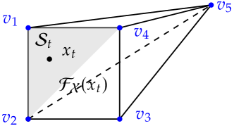
Figure 22: Trajectory dependence of the AFW algorithm: We depict the vertices that define the polytope $\mathcal{X}$ in blue, that is, $\mathcal{X}=\operatorname{conv}(\{v_{1},v_{2},v_{3},v_{4},v_{5}\})$. Note that the smallest face containing $x_{t}$ is $\mathcal{F}_{\mathcal{X}}(x_{t})=\operatorname{conv}(\{v_{1},v_{2},v_{3},v_{4}\})$. The region shaded in grey indicates the convex hull of the active set $\mathcal{S}_{t}=\{v_{1},v_{2},v_{4}\}$, i.e. $\operatorname{conv}(\mathcal{S}_{t})$. Note that the iterate $x_{t}$ can be written as a convex combination of the elements in $\mathcal{S}_{t}$, or as a convex combination of the vertices in $\mathcal{F}_{\mathcal{X}}(x_{t})$, as such, the away-step in the AFW algorithm will depend on how we write $x_{t}$ as a convex decomposition. This means that the step taken by the AFW algorithm a at iteration $t$ depends on the vertices that have been picked up in previous iterations, making it trajectory dependent.

Let $\mathcal{F}_{\mathcal{X}}(x_{t})$ denote the smallest face of $\mathcal{X}$ containing $x_{t}$. Clearly $\operatorname{conv}(\mathcal{S}_{t})\subseteq\mathcal{F}_{\mathcal{X}}(x_{t})$, and in many cases there can potentially be multiple active sets such that $x_{t}\in\mathcal{S}_{t}$. In the example shown in Figure 22 the point $x_{t}$ can be represented as the convex combination of $\mathcal{S}_{t}=\{v_{1},v_{2},v_{4}\}$ (as is shown in the image in light gray), or as a convex combination of the vertices of $\mathcal{F}_{\mathcal{X}}(x_{t})$, that is, $\operatorname{Vert}(\mathcal{F}_{\mathcal{X}}(x_{t}))=\{v_{1},v_{2},v_{3},v_{4}\}$, as such the away step taken by the AFW algorithm (Algorithm 2) will depend on $\mathcal{S}_{t}$. The Extended Frank–Wolfe Method with "In-face directions" (Algorithm 20) from [98] attempts to generalize the notion of away steps from [114], giving greater control over the sparsity of the generated solutions through two preference parameters, namely $\alpha_{1}$ and $\alpha_{2}$. For example, small values of $\alpha_{1}$ and $\alpha_{2}$ in Algorithm 20 promote sparsity over reduction in function value, which is especially beneficial in matrix completion problems, where sparsity translates to low rank of the solution as a matrix, which can be important, e.g., when solving matrix completion problems.

Algorithm 20 In-Face Extended Frank–Wolfe [98]

0   Start atom $x_{0}\in\mathcal{X}$, initial lower bound $B_{-1}\leq f(x^{*})$, and parameters $0\leq\alpha_{1}\leq\alpha_{2}\leq 1$

0   Iterates $x_{1},\dotsc\in\mathcal{X}$

1   for $t=0$ to … do

2      $B_{t}\leftarrow B_{t-1}$

3       Choose $d_{t}$ with $x_{t}-d_{t}\in\operatorname*{Aff}\left(\mathcal{F}_{\mathcal{X}}(x_{t})\right)$ and $\mathinner{{}\langle\nabla f(x_{t}),d_{t}\rangle}\geq 0$.

4      $\gamma_{\max}\leftarrow\operatorname*{argmax}_{\gamma}\{\gamma\mid x_{t}-\gamma d_{t}\in\mathcal{F}_{\mathcal{X}}(x_{t})\}$

5      $x_{t}^{B}\leftarrow x_{t}-\gamma_{\max}d_{t}$

6       $x_{t}^{A}\leftarrow x_{t}-\tilde{\gamma}d_{t}$ where $\tilde{\gamma}\in[0,\gamma_{\max}]$

7      if $\frac{2LD^{2}}{2LD^{2}+\alpha_{1}\left(f(x_{t})-B_{t}\right)}\left(f(x_{t})-B_{t}\right)\geq f(x_{t}^{B})-B_{t}$ then

8         $x_{t+1}\leftarrow x_{t}^{B}$ {Go to lower dimensional face.}

9      else if $\frac{2LD^{2}}{2LD^{2}+\alpha_{2}\left(f(x_{t})-B_{t}\right)}\left(f(x_{t})-B_{t}\right)\geq f(x_{t}^{A})-B_{t}$ then

10         $x_{t+1}\leftarrow x_{t}^{A}$ {Stay in current face.}

11      else

12         $v_{t}^{\text{FW}}\leftarrow\operatorname*{argmin}_{v\in\mathcal{X}}\mathinner{{}\langle\nabla f(x_{t}),v\rangle}$ {Frank–Wolfe step}

13         $x_{t+1}\leftarrow x_{t}+\hat{\gamma}(v_{t}-x_{t})$ with $\hat{\gamma}\in[0,1]$

14         $B_{t}\leftarrow\max\{B_{t-1},f(x_{t})+\mathinner{{}\langle\nabla f(x_{t}),v_{t}-x_{t}\rangle}\}$

15      end if

16   end for

The In-Face Extended Frank–Wolfe Method algorithm (Algorithm 20) assumes that it is possible to work with the minimal face $\mathcal{F}_{\mathcal{X}}(x_{t})$. This is the case for example when minimizing over the spectrahedron, but it is usually not possible in general, and is a limiting assumption for this algorithm. Note that the quantity $B_{t}$ maintained during the run of the algorithm is a lower bound in $f(x^{*})$, and used throughout the algorithm to decide which type of steps to perform, either steps that remain in $\mathcal{F}_{\mathcal{X}}(x_{t})$, or steps that can potentially leave $\mathcal{F}_{\mathcal{X}}(x_{t})$.

At each iteration the algorithm chooses between three improving strategies with a preference to solutions in lower dimensional faces. The most preferred strategy is moving to a subface of the minimal face (Line 8), followed by staying within the minimal face (Line 10); these two together generalize away steps. The third algorithm is a fallback strategy: a standard Frank–Wolfe step (with no restrictions on the solution). The preference is expressed by requiring less progress from more preferred strategies. The parameters $\alpha_{1}$ and $\alpha_{2}$ quantify the degree of preference of the strategies in the conditions in Line 7 and Line 9. Note that $B_{t}\leq f(x^{*})$, and so $f(x_{t})-B_{t}\geq f(x_{t})-f(x^{*})\geq 0$, which means that the multiplicative factors $2LD^{2}/(2LD^{2}+\alpha_{1}\left(f(x_{t})-B_{t}\right))$ and $2LD^{2}/(2LD^{2}+\alpha_{2}\left(f(x_{t})-B_{t}\right))$ are both smaller than $1$ (while the former is smaller than the latter as $\alpha_{2}\geq\alpha_{1}$). This means that the if $\alpha_{1}$ is large, in order to move to $x_{t}^{B}$ in Line 8 we will require that the reduction in function value from moving to $x_{t}^{B}$ be large (as the factor $2LD^{2}/(2LD^{2}+\alpha_{1}\left(f(x_{t})-B_{t}\right))$ will be small), compared to staying in $x_{t}$. Similarly if $\alpha_{1}$ is small, we will not require a large reduction in function value from moving to $x_{t}^{B}$, compared to staying in $x_{t}$. At a high-level if $\alpha_{1}$ is large we prioritize decreasing the function value over iterations, whereas if $\alpha_{1}$ is small we prioritize sparsity. Similar comments can be made regarding the condition in Line 9.

The first two strategies also search for improving solutions in only one direction $d_{t}$ like a Frank–Wolfe step. There are two recommendation for choosing $d_{t}$ in Line 3: the analogue of away steps over $\mathcal{F}_{\mathcal{X}}(x_{t})$, namely $d_{t}=v-x_{t}$, where $v=\operatorname*{argmax}_{v\in\mathcal{F}_{\mathcal{X}}(x_{t})}\mathinner{{}\langle\nabla f(x_{t}),v\rangle}$, and a Frank–Wolfe step on $\mathcal{F}_{\mathcal{X}}(x_{t})$, that is $d_{t}=u-x_{t}$, where $u=\operatorname*{argmin}_{v\in\mathcal{F}_{\mathcal{X}}(x_{t})}\mathinner{{}\langle\nabla f(x_{t}),v\rangle}$. Or, as [98] suggest, one could even attempt to find the minimum of $f$ over $\mathcal{F}_{\mathcal{X}}(x_{t})$, and use $d_{t}=w-x_{t}$, where $w=\operatorname*{argmin}_{v\in\mathcal{F}_{\mathcal{X}}(x_{t})}f(v)$. The three aforementioned strategies all require access to $\mathcal{F}_{\mathcal{X}}(x_{t})$.

The convergence rate in [98] for Algorithm 20 is roughly of the form $\mathcal{O}(LD^{2}/t)$ after $t$ iterations. The overall effect of $\alpha_{1}$ and $\alpha_{2}$ on sparsity and convergence rate is unclear. Unlike the AFW algorithm, due to the algorithmic setup, the algorithm may omit the LP oracle call over the whole feasible region in some iterations. When working with the minimal face directly is too expensive, a good compromise with similar control over sparsity versus function value decrease is the Blended Conditional Gradient algorithm in Section 9.2 that works with a specific decomposition and does not rely on access to $\mathcal{F}_{\mathcal{X}}(x)$.

4 Conditional gradients in the large-scale setting

We will now focus on conditional gradient methods for large-scale settings, where access to the exact value of the objective function or its gradient is computationally prohibitive. We start by considering stochastic gradients (Section 10) where, instead of exact gradients, (ostensibly cheaper) gradient estimators with some random noise are used. This is typical for stochastic optimization, in which the objective function that is the expected value of some random function (Section 10). We also study a special case of this problem where the objective function is defined as the sum of a finite number of functions, also known as finite-sum optimization.

In distributed optimization (Section 12), communication is a new scarce resource required for function access. In particular, the components of the objective function are distributed over a set of nodes, which thus have to share information to compute, e.g., the gradient of the objective function. Hence, one needs to design a set of algorithms that can be implemented in a decentralized manner. We discuss conditional gradient algorithms that exploit only local and neighboring information to find a suitable descent direction.

In Section 11 we examine conditional gradient methods for online optimization, which adds a time dimension to the problem: we optimize objective functions, which will be only revealed in the future. We study a class of dynamic conditional gradient variants that exploit information from prior objective functions.

10 Conditional gradients for stochastic optimization

In this section, we focus on the extension of Frank–Wolfe methods to stochastic optimization problems. Here the goal is to minimize an objective function which is defined through an expectation over a set of functions. The main challenge arises from the fact that typically the cost of computing the objective value or its gradient is much more expensive than computing the same quantities for the individual underlying functions. Stochastic optimization problems appear naturally in several areas, including machine learning [34, see, e.g.,], adaptive filters [120], and portfolio selection [231].

We consider a function $\tilde{F}\colon\mathcal{X}\times\mathcal{Z}\to\mathbb{R}$ together with a random variable $Z\in\mathcal{Z}$. We assume that the function $\tilde{F}$ is smooth and convex in its first variable $x\in\mathcal{X}$ unless stated otherwise. The goal is to minimize the expectation of $\tilde{F}(\cdot,Z)$, which is formally defined as the objective function $f$:

$$\min_{x\in\mathcal{X}}f(x)\quad\text{where}\quad f(x)\stackrel{{\scriptstyle\textnormal{\scriptsize def}}}{{=}}\mathop{\mathbb{E}}\nolimits\left[\tilde{F}(x,Z)\right].$$ (152)

In the above expression, the expectation is over the randomness of $Z$.

Example 4.1.

A classic example of a stochastic optimization problem is a supervised␣learning problem defined by an expected risk minimization. In this setting the data points to learn from are pairs $(z,y)$ of an input or feature vector $z$ and an output or label $y$. The data are encoded by a random variable $Z$ over the data points. The goal is to find a map $x$ on the inputs $z$ predict the outputs $y$. The most simple case is a linear model where $x$ is a linear function, which can be formulated as

$$\min f(x)=\mathop{\mathbb{E}}\nolimits_{(z,y)\sim Z}\left[\ell(\mathinner{{}\langle x,z\rangle},y)\right],$$

where the loss function $\ell\colon\mathbb{R}^{n}\to\mathbb{R}$ measures the gap between the predicted label $\mathinner{{}\langle x,z\rangle}$ and the true label $y$. Note that this is a stochastic optimization problem in the form of (152) with $\tilde{F}(x,(z,y))\stackrel{{\scriptstyle\textnormal{\scriptsize def}}}{{=}}\ell(\mathinner{{}\langle x,z\rangle},y)$. A common choice for the loss function $\ell$ is the quadratic loss which leads to the following problem

$$\min f(x)=\mathop{\mathbb{E}}\nolimits_{(z,y)\sim Z}\left[\mathinner{{}\lVert\mathinner{{}\langle x,z\rangle}-y\rVert}_{2}^{2}\right].$$

We assume that the distribution of $Z$ is independent of $x$, which is called the oblivious setting. A more general version of the above problem is the non-oblivious setting in which the underlying distribution of $Z$ depends on the variable $x$ and may change during the optimization procedure. Non-oblivious stochastic optimization appears naturallly in several problem classes, such as, e.g., multilinear extension of a discrete submodular function, Maximum a Posteriori (MAP) inference in determinantal point processes, and policy gradients in reinforcement learning. In this section, we shall not consider the non-oblivious setting, but we should highlight that most algorithms for the oblivious setting work equally well in the non-oblivious setting.

While we will assume that the expected function $f$ is smooth, with the exception of Section 10.5, the individual functions $\tilde{F}(\cdot,z)$ need not be smooth. All algorithms presented in this section aim at avoiding the expensive task of computing the exact gradient $\nabla f$ of the objective function by utilizing some sort of a gradient estimator $\mathaccent 0{\symlargesymbols}065{\nabla}f$. This results in the basic template shown in Template 1 for stochastic Frank–Wolfe algorithms. The idea of using a gradient estimator instead of the true gradient has been extensively investigated for projected gradient decent and resulted in the popular stochastic gradient descent methodology. The idea of using gradient estimation was first proposed in the context of Markov chains by [219].

Algorithm 1 Stochastic Conditional Gradient

0   Start point $x_{0}\in\mathcal{X}$, step-sizes $0\leq\gamma_{t}\leq 1$.

1   for $t=0$ to … do

2      Compute gradient estimator $\mathaccent 0{\symlargesymbols}065{\nabla}f(x_{t})$

3      $v_{t}\leftarrow\operatorname*{argmin}_{v\in\mathcal{X}}\mathinner{{}\langle\mathaccent 0{\symlargesymbols}065{\nabla}f(x_{t}),v\rangle}$

4      $x_{t+1}\leftarrow x_{t}+\gamma_{t}(v_{t}-x_{t})$

5   end for

The simplest gradient estimator is the stochastic␣gradient $\nabla\tilde{F}(x,z)$ for a realization $z$ of the random variable $Z$, which is known as the Stochastic First-Order Oracle (SFOO), shown in Oracle 2.

Algorithm 2 Stochastic First-Order Oracle for $f$ (SFOO)

0   Point $x\in\mathcal{X}$

0   $\mathaccent 0{\symlargesymbols}065{\nabla}f(x)\leftarrow\nabla\tilde{F}(x,z)$, where $z$ is an independent realization of $Z$

In order to quantify the accuracy of the stochastic first-order oracle, we make the following assumption throughout this section, which is standard in the stochastic optimization literature. Throughout this section, the norm will be always the Euclidean norm, i.e., the $\ell_{2}$-norm.

Assumption 4.2.

There is a $\sigma^{2}>0$ such that the variance of the stochastic gradient samples is bounded by $\sigma^{2}$, i.e., for all $x\in\mathcal{X}$, i.e., $\mathop{\mathbb{E}}\nolimits\left[\mathinner{{}\lVert\nabla\tilde{F}(x,Z)-\nabla f(x)\rVert}^{2}\right]\leq\sigma^{2}$.

Remark 4.3 (Frank–Wolfe vertices become biased).

The main difficulties of stochastic conditional gradients algorithms arise from the fact that Frank–Wolfe vertex of even an unbiased gradient estimator is usually a biased estimator of the Frank–Wolfe vertex. As a simple example, let $Z$ be a uniformly distributed random variable over $\{-1,+1\}$, i.e., $\mathop{\mathbb{P}}\nolimits\left[Z=-1\right]=\mathop{\mathbb{P}}\nolimits\left[Z=+1\right]=1/2$. Let us consider $\smash{f(x)\stackrel{{\scriptstyle\textnormal{\scriptsize def}}}{{=}}\mathop{\mathbb{E}}\nolimits\left[(x-x^{*}+Z)^{2}\right]}=(x-x^{*})^{2}+1$ over the interval $[0,1]$ for a constant $0<a<1$. Now at any $0\leq x\leq 1$ the Frank–Wolfe vertex of the stochastic gradient $\mathaccent 0{\symlargesymbols}065{\nabla}f(x)=2(x-x^{*}+Z)$, is uniformly distributed over $\{0,1\}$, and hence holds no information about $x^{*}$.

This simple example highlights that the core of the Frank–Wolfe algorithm, linear minimization, is sensitive to accuracy, and introduces bias: $\mathop{\mathbb{E}}\nolimits\left[\min_{v\in\mathcal{X}}\mathinner{{}\langle\tilde{\nabla},v\rangle}\right]\neq\min_{v\in\mathcal{X}}\mathinner{{}\langle\mathop{\mathbb{E}}\nolimits\left[\tilde{\nabla}\right],v\rangle}$, where $\tilde{\nabla}$ is a random vector. Stochastic Frank–Wolfe algorithms counteract this by increasing accuracy of gradient estimators. This is a drawback compared to stochastic projected gradient descent methods.

We shall use $\mathop{\mathbb{E}}\nolimits_{t}\left[\cdot\right]$, $\mathop{\mathbb{V}}\nolimits_{t}\left[\cdot\right]$ to denote the conditional expectation and variance given the run of the algorithm till the end of computation of iterate $x_{t}$. The following lemma quantifies how the accuracy of the gradient estimate $\mathaccent 0{\symlargesymbols}065{\nabla}f(x_{t})$ affects the progress made in a single step.

Lemma 4.4.

If $f$ is an $L$-smooth convex function on a compact convex set $\mathcal{X}$ with diameter at most $D$, then for all $t\geq 0$ the iterates of Template 1 satisfy the following

$$\begin{multlined}\mathop{\mathbb{E}}\nolimits\left[f(x_{t+1})-f(x^{*})\right]\\[-4.30554pt] \leq(1-\gamma_{t})\mathop{\mathbb{E}}\nolimits\left[f(x_{t})-f(x^{*})\right]+\gamma_{t}\smash[t]{\sqrt{\mathop{\mathbb{E}}\nolimits\left[\mathinner{{}\lVert\mathaccent 0{\symlargesymbols}065{\nabla}f(x_{t})-\nabla f(x_{t})\rVert}^{2}\right]}}D+\frac{LD^{2}}{2}\gamma_{t}^{2},\end{multlined}\mathop{\mathbb{E}}\nolimits\left[f(x_{t+1})-f(x^{*})\right]\\[-4.30554pt] \leq(1-\gamma_{t})\mathop{\mathbb{E}}\nolimits\left[f(x_{t})-f(x^{*})\right]+\gamma_{t}\smash[t]{\sqrt{\mathop{\mathbb{E}}\nolimits\left[\mathinner{{}\lVert\mathaccent 0{\symlargesymbols}065{\nabla}f(x_{t})-\nabla f(x_{t})\rVert}^{2}\right]}}D+\frac{LD^{2}}{2}\gamma_{t}^{2},$$ (155)

$$\begin{multlined}\mathop{\mathbb{E}}\nolimits\left[f(x_{t+1})-f(x_{t})\right]\\[-4.30554pt] \leq-\gamma_{t}\mathop{\mathbb{E}}\nolimits\left[g(x_{t})\right]+\gamma_{t}\smash[t]{\sqrt{\mathop{\mathbb{E}}\nolimits\left[\mathinner{{}\lVert\mathaccent 0{\symlargesymbols}065{\nabla}f(x_{t})-\nabla f(x_{t})\rVert}^{2}\right]}}D+\frac{LD^{2}}{2}\gamma_{t}^{2},\end{multlined}\mathop{\mathbb{E}}\nolimits\left[f(x_{t+1})-f(x_{t})\right]\\[-4.30554pt] \leq-\gamma_{t}\mathop{\mathbb{E}}\nolimits\left[g(x_{t})\right]+\gamma_{t}\smash[t]{\sqrt{\mathop{\mathbb{E}}\nolimits\left[\mathinner{{}\lVert\mathaccent 0{\symlargesymbols}065{\nabla}f(x_{t})-\nabla f(x_{t})\rVert}^{2}\right]}}D+\frac{LD^{2}}{2}\gamma_{t}^{2},$$ (158)

where $g(x)=\max_{v\in\mathcal{X}}\mathinner{{}\langle\nabla f(x),x-v\rangle}$ is the Frank–Wolfe gap (Definition 1.11). The second inequality does not require convexity of $f$ as long as it is smooth. Moreover, these inequalities also hold for conditional expectation, i.e., by replacing $\mathop{\mathbb{E}}\nolimits\left[\cdot\right]$ with $\mathop{\mathbb{E}}\nolimits_{t}\left[\cdot\right]$ on the left-hand side, and with the identity function on the right-hand side.

Note that the key difference to the non-stochastic version in Lemma 1.5 is the extra term measuring the accuracy of stochastic gradients:

$$\gamma_{t}\sqrt{\mathop{\mathbb{E}}\nolimits\left[\mathinner{{}\lVert\mathaccent 0{\symlargesymbols}065{\nabla}f(x_{t})-\nabla f(x_{t})\rVert}^{2}\right]}D.$$

Controlling this term is key to obtaining good convergence rates.

Proof of Lemma 4.4.

The first inequality easily follows from the second inequality, as $f(x_{t})-f(x^{*})\leq g(x_{t})$ for convex $f$, see Equation (16). Hence, we prove only the second one. The key is to estimate the error due to the approximation of the gradient, using the optimality of $v_{t}$:

$$\begin{split}g(x_{t})+\mathinner{{}\langle\nabla f(x_{t}),v_{t}-x_{t}\rangle}&=\max_{v\in\mathcal{X}}\mathinner{{}\langle\nabla f(x_{t}),v_{t}-v\rangle}\\ &\leq\max_{v\in\mathcal{X}}\mathinner{{}\langle\mathaccent 0{\symlargesymbols}065{\nabla}f(x_{t}),v_{t}-v\rangle}+\max_{v\in\mathcal{X}}\mathinner{{}\langle\nabla f(x_{t})-\mathaccent 0{\symlargesymbols}065{\nabla}f(x_{t}),v_{t}-v\rangle}\\ &\leq\mathinner{{}\lVert\nabla f(x_{t})-\mathaccent 0{\symlargesymbols}065{\nabla}f(x_{t})\rVert}D,\end{split}$$

where the last inequality follows by using the fact that $v_{t}=\operatorname*{argmin}_{v\in\mathcal{X}}\mathinner{{}\langle\mathaccent 0{\symlargesymbols}065{\nabla}f(x_{t}),v\rangle}$ as well as the Cauchy-Shwarz inequality. We combine this with the standard progress estimation, using smoothness of $f$ (see Lemma 1.5):

$$\begin{split}f(x_{t+1})-f(x_{t})&\leq\gamma_{t}\mathinner{{}\langle\nabla f(x_{t}),v_{t}-x_{t}\rangle}+\frac{L}{2}\gamma_{t}^{2}\mathinner{{}\lVert v_{t}-x_{t}\rVert}^{2}\\ &\leq-\gamma_{t}g(x_{t})+\gamma_{t}\mathinner{{}\lVert\mathaccent 0{\symlargesymbols}065{\nabla}f(x_{t})-\nabla f(x_{t})\rVert}D+\frac{LD^{2}}{2}\gamma_{t}^{2}.\end{split}$$

The proof concludes by taking expectations, and using the following application of Jensen’s inequality to bound the expectation of the error of the stochastic gradient:

$$\mathop{\mathbb{E}}\nolimits\left[\mathinner{{}\lVert\mathaccent 0{\symlargesymbols}065{\nabla}f(x_{t})-\nabla f(x_{t})\rVert}\right]\leq\sqrt{\mathop{\mathbb{E}}\nolimits\left[\mathinner{{}\lVert\mathaccent 0{\symlargesymbols}065{\nabla}f(x_{t})-\nabla f(x_{t})\rVert}^{2}\right]}.\qed$$

We include here an application appearing in many proofs below for the agnostic step size rule $\gamma_{t}=2/(t+2)$.

Lemma 4.5.

Let $f$ be an $L$-smooth convex function on a compact convex set $\mathcal{X}$, with diameter $D$. In Template 1 let the step sizes be $\gamma_{t}=2/(t+2)$. Assume that the stochastic gradients satisfy

$$\sqrt{\mathop{\mathbb{E}}\nolimits\left[\mathinner{{}\lVert\mathaccent 0{\symlargesymbols}065{\nabla}f(x_{t})-\nabla f(x_{t})\rVert}^{2}\right]}\leq G\gamma_{t}.$$ (159)

Then the iterates $x_{t}$ satisfy

$$\mathop{\mathbb{E}}\nolimits\left[f(x_{t})-f(x^{*})\right]\leq\frac{4GD+2LD^{2}}{t+2}.$$ (160)

(Here as an exception. $G$ is not necessarily an upper bound on the size of gradient of $f$.)

Proof.

Plugging (159) into Lemma 4.4 we obtain

$$\mathop{\mathbb{E}}\nolimits\left[f(x_{t+1})-f(x^{*})\right]\leq(1-\gamma_{t})\mathop{\mathbb{E}}\nolimits\left[f(x_{t})-f(x^{*})\right]+\frac{2GD+LD^{2}}{2}\gamma_{t}^{2}.$$ (161)

We conclude the proof by induction. Let $Q\stackrel{{\scriptstyle\textnormal{\scriptsize def}}}{{=}}4GD+2LD^{2}$, so that the claim becomes $\mathop{\mathbb{E}}\nolimits\left[f(x_{t})-f(x^{*})\right]\leq Q/(t+2)$. As $\gamma_{0}=1$, we have that $\mathop{\mathbb{E}}\nolimits\left[f(x_{1})-f(x^{*})\right]\leq Q/4$ by application of Equation (161). Hence (164) holds for $t=1$. Suppose (164) holds for some $t$. By (161), we have

$$\begin{split}\mathop{\mathbb{E}}\nolimits\left[f(x_{t+1})-f(x^{*})\right]&\leq\left(1-\frac{2}{t+2}\right)\frac{Q}{t+2}+\frac{Q}{(t+2)^{2}}\\ &=\frac{Q(t+1)}{(t+2)^{2}}\\ &\leq\frac{Q}{t+3}\end{split}$$

by $(t+1)(t+3)\leq(t+2)^{2}$. ∎

The accuracy of the gradient estimation plays a key role in how fast stochastic optimization methods converge. This explains why estimators built from a few number of stochastic gradients but with significantly smaller variance have received a lot of attention over the past few years, primarily for stochastic gradient descent methods. Some of these estimators will be mentioned in later sections.

A simple way to obtain more accurate estimates of the gradient is by computing the average over a finite number of independent samples. More precisely, we can construct a simple unbiased gradient estimator with improved accuracy by drawing independent samples $z_{1},\dotsc,z_{b}$ of $Z$ and computing:

$$\mathaccent 0{\symlargesymbols}065{\nabla}f(x)=\frac{1}{b}\sumop\slimits@_{j=1}^{b}\nabla\tilde{F}(x,z_{j}).$$ (162)

It is easy to verify that the variance of such estimator is a factor $b$ less compared to the single simple estimate for the case $b=1$. This technique is used to increase the accuracy of the estimators as the algorithm progresses.

We close this section by remarking that the stochastic problem in (152) appears ubiquitously in many domains, however, an important special case of it is when the randomness has a finite support.

Remark 4.6 (The case of finite-sum minimization).

The constrained finite-sum problem

$$\min_{x\in\mathcal{X}}\frac{1}{m}\sumop\slimits@_{i=1}^{m}f_{i}(x)$$ (163)

is a special case of Problem (152) where $\mathcal{X}$ is a compact convex set and $f_{1},\dotsc,f_{m}\colon\mathcal{X}\to\mathbb{R}$ are smooth, possibly non-convex functions, via the choices $\tilde{F}(x,z)\stackrel{{\scriptstyle\textnormal{\scriptsize def}}}{{=}}f_{z}(x)$ and $Z$ a uniform random variable over $\{1,2,\dotsc,m\}$. This setting is quite ubiquitous in machine learning, as many learning problems are formulated via empirical risk minimization, which is of this form. As such, all results of the more general Problem (152) also apply to finite-sum minimization, hence we will only explicitly mention results on finite-sum minimization, where the finite-sum structure leads to improvement.

10.1 Stochastic first-order oracle complexity

Here we recall some of the known complexity lower bounds for stochastic first-order methods. For a maximum expected primal gap error $\varepsilon>0$ the lower bounds are summarized in Table 4. Note that here the only accuracy constraint on stochastic gradients is that they are bounded, while most convergence results in this chapter use a weaker assumption that only the variance of the stochastic gradients are bounded.

Table 4: Minimum number of stochastic first-order oracle calls to optimize a convex objective function up to an expected primal gap of at most $\varepsilon>0$, where the worst-case examples depend on $\varepsilon$. The feasible region is $n$-dimensional and contains an $\ell_{\infty}$-ball of radius $r>0$. The stochastic gradients are assumed to be unbiased and bounded by $G$ in the dual of the $\ell_{p}$-norm [2, Theorems 1 and 2].

Objective function	Stochastic FOO calls	Restrictions
$G$-Lipschitz in $\ell_{p}$-norm	$\Omega\bigl{(}(Grn^{\max\{1/2,1/p\}}/\varepsilon)^{2}\bigr{)}$
$G$-Lipschitz in $\ell_{p}$-norm, $\mu$-strongly convex in $\ell_{2}$-norm	$\Omega\bigl{(}G^{2}n^{2/p-1}/(\mu^{2}\varepsilon)\bigr{)}$	$1\leq p<2$
$G$-Lipschitz in $\ell_{p}$-norm, $\mu$-strongly convex in $\ell_{2}$-norm	$\Omega\bigl{(}G^{2}/(\mu^{2}\varepsilon)\bigr{)}$	$p=\infty$

The authors are not aware of a lower bound on the number required stochastic oracle calls for finding a point with a Frank–Wolfe gap of $\varepsilon$ for constrained problems, but for completeness, we would like to state that the analogous version of the above goal for unconstrained optimization problems, which is obtaining a solution $x$ with $\mathinner{{}\lVert\nabla f(x)\rVert}_{*}\leq\varepsilon$ requires at least $\Omega(\sqrt{Lh_{0}}/\varepsilon+(\sigma^{2}/\varepsilon^{2})\log(Lh_{0}/\varepsilon^{2}))$ stochastic first-order oracle calls in the worst-case depending on $\varepsilon$ [96, Theorem 2], where $L$ is the objective function smoothness parameter and $\sigma^{2}$ is an upper bound on the stochastic oracle of variance. Here as usual $h_{0}$ is the primal gap error of the starting point.

10.2 Stochastic Frank–Wolfe algorithm

As mentioned above, the most natural extension of the FW algorithm for stochastic optimization is obtained by replacing the gradient in the update with its stochastic approximation, as suggested in [123]. We formally present this algorithm in Algorithm 3. Note that the batch sizes $b_{t}$ are input parameters of this algorithm, to allow for gradient estimators that increase in accuracy during the run of the algorithm. In the next theorem we formally state the convergence rate of this algorithm.

Algorithm 3 Stochastic Frank–Wolfe (SFW) [123]

0   Arbitrary start point $x_{0}\in\mathcal{X}$, batch sizes $b_{t}$, step sizes $0\leq\gamma_{t}\leq 1$ for $t\geq 0$

0   Iterates $x_{1},\dotsc\in\mathcal{X}$

1   for $t=0$ to … do

2      Draw $\{z_{1},\dotsc,z_{b_{t}}\}$, that is, $b_{t}$ independent realizations of $Z$.

3       $\mathaccent 0{\symlargesymbols}065{\nabla}f(x_{t})\leftarrow\frac{1}{b_{t}}\sumop\slimits@_{j=1}^{b_{t}}\nabla\tilde{F}(x_{t},z_{j})$

4      $v_{t}\leftarrow\operatorname*{argmin}_{v\in\mathcal{X}}\mathinner{{}\langle\mathaccent 0{\symlargesymbols}065{\nabla}f(x_{t}),v\rangle}$

5      $x_{t+1}\leftarrow x_{t}+\gamma_{t}(v_{t}-x_{t})$

6   end for

Theorem 4.7.

Let $f$ be a convex, $L$-smooth function over a convex compact set $\mathcal{X}$ with diameter at most $D$. If the stochastic gradient samples of $f$ have variance of at most $\sigma^{2}$, then the Stochastic Frank–Wolfe algorithm (Algorithm 3) with batch sizes $b_{t}\stackrel{{\scriptstyle\textnormal{\scriptsize def}}}{{=}}(t+2)^{2}/\alpha$ for a fixed $\alpha>0$ and step sizes $\gamma_{t}\stackrel{{\scriptstyle\textnormal{\scriptsize def}}}{{=}}2/(t+2)$, ensures for all $t\geq 1$

$$\mathop{\mathbb{E}}\nolimits\left[f(x_{t})\right]-f(x^{*})\leq\frac{2(\sqrt{\alpha}\sigma D+LD^{2})}{t+2}.$$ (164)

Equivalently, to achieve an expected primal gap $\mathop{\mathbb{E}}\nolimits\left[f(x_{t})\right]-f(x^{*})\leq\varepsilon$, for $\varepsilon>0$, the Stochastic Frank–Wolfe algorithm (Algorithm 3) computes $\mathcal{O}((\sqrt{\alpha}\sigma D+LD^{2})^{3}/(\alpha\varepsilon^{3}))$ stochastic gradients and performs $\mathcal{O}((\sqrt{\alpha}\sigma D+LD^{2})/\varepsilon)$ linear minimizations.

For the sake of comparison, we note that the projected stochastic gradient descent uses $\mathcal{O}(G^{2}D^{2}/\varepsilon^{2})$ stochastic gradients for an expected primal gap at of most $\varepsilon>0$, where $G^{2}$ is an upper bound on the second moment $\mathop{\mathbb{E}}\nolimits\left[\mathinner{{}\lVert\nabla\tilde{F}(x,z)\rVert}^{2}\right]\leq G^{2}$ of the stochastic gradients, see [187, Eq. (2.18) ]

We should also add that in the original paper [123], the parameter $\alpha$ is selected as $\alpha=\left(LD/\sigma\right)^{2}$, which is obtained by minimizing the upper bound of the linear minimizations performed. However, here we have presented a slightly more general form of this result to highlight that a parameter-free choice like $\alpha=1$ has the same convergence bound up to a constant factor that depends on some parameters of the objective function.

Proof.

We will use Lemma 4.5 to prove the bound. In order to do so we need to bound $\mathinner{{}\lVert\mathaccent 0{\symlargesymbols}065{\nabla}f(x_{t})-\nabla f(x_{t})\rVert}$. Since the samples are drawn i.i.d., the variance of $\mathaccent 0{\symlargesymbols}065{\nabla}f(x_{t})$ is bounded from above by $\mathop{\mathbb{E}}\nolimits\left[\mathinner{{}\lVert\mathaccent 0{\symlargesymbols}065{\nabla}f(x_{t})-\nabla f(x_{t})\rVert}^{2}\right]\leq\frac{\sigma^{2}}{b_{t}}$. Thus using the values of $b_{t}$ and $\gamma_{t}$ provided in the statement of the theorem we obtain

$$\sqrt{\mathop{\mathbb{E}}\nolimits\left[\mathinner{{}\lVert\mathaccent 0{\symlargesymbols}065{\nabla}f(x_{t})-\nabla f(x_{t})\rVert}^{2}\right]}\leq\frac{\sigma}{\sqrt{b_{t}}}=\frac{\sqrt{\alpha}\sigma}{t+2}=\frac{\sqrt{\alpha}\sigma}{2}\gamma_{t}.$$

The claim follows by Lemma 4.5 with the choice $G\stackrel{{\scriptstyle\textnormal{\scriptsize def}}}{{=}}\sqrt{\alpha}\sigma/2$. ∎

We now turn our attention to the case where $f$ is not convex. In the deterministic setting (Section 6.3), the minimal Frank–Wolfe gap $g(x_{t})$ of all iterates $x_{t}$ is used as an accuracy measure, with the implicit understanding that an iterate realizing the minimal gap is chosen as the final solution. In the stochastic setting, together with the exact gradients $\nabla f(x_{t})$ of the iterates, the Frank–Wolfe gaps are expensive to compute, too, requiring a different choice of final solution. We examine the common choice of a uniformly random selection from the generated iterates, thus the expected Frank–Wolfe gap becomes the average of the expected Frank–Wolfe gaps of the individual iterates: $\sumop\slimits@_{\tau=0}^{t-1}\mathop{\mathbb{E}}\nolimits\left[g(x_{\tau})\right]/t$.

Theorem 4.8(i) follows from [217] and assumes a fixed time horizon. Alternatively, Theorem 4.8(ii) presents a slightly slower convergence rate as done in [70] but does not require a fixed time horizon.

Theorem 4.8.

Let $f$ be an $L$-smooth (and not necessarily convex) function on a compact convex set $\mathcal{X}$ with diameter at most $D$. Consider SFW (Algorithm 3) with stochastic gradients of variance at most $\sigma^{2}$.

1. If $b_{t}=(\sigma/(LD))^{2}T$ and $\gamma_{t}=1/\sqrt{T}$, for all $0\leq t\leq T-1$, then

   $$\frac{1}{T}\sumop\slimits@_{t=0}^{T-1}\mathop{\mathbb{E}}\nolimits\left[g(x_{t})\right]\leq\frac{\bigl{(}f(x_{0})-f(x^{*})\bigr{)}+(3/2)LD^{2}}{\sqrt{T}}.$$

   Equivalently, for an expected Frank–Wolfe gap at most $\varepsilon>0$, the Stochastic Frank–Wolfe algorithm (Algorithm 3) computes $\mathcal{O}(\sigma^{2}L^{2}D^{4}/\varepsilon^{4})$ stochastic gradients and performs $\mathcal{O}(L^{2}D^{4}/\varepsilon^{2})$ linear minimizations over the feasible region, running $T=L^{2}D^{4}/\varepsilon^{2}$ iterations of the algorithm, and choosing one of the iterates $x_{0}$, …, $x_{T}$ uniformly randomly as the final solution.

2. If $b_{t}=(\sigma/(LD))^{2}(t+1)$ and $\gamma_{t}=1/(t+1)^{1/2+\nu}$ for a parameter $0<\nu<1/2$, then for all $t\geq 1$

   $$\frac{1}{t}\sumop\slimits@_{\tau=0}^{t-1}\mathop{\mathbb{E}}\nolimits\left[g(x_{\tau})\right]\leq\frac{\bigl{(}f(x_{0})-f(x^{*})\bigr{)}+(3/2)LD^{2}\zeta(1+\nu)}{t^{1/2-\nu}},$$

   where $\zeta(\nu)\stackrel{{\scriptstyle\textnormal{\scriptsize def}}}{{=}}\sumop\slimits@_{s=0}^{+\infty}1/(s+1)^{\nu}\in\mathbb{R}_{+}$ is the Riemann zeta function.

Remark 4.9.

In Theorem 4.8(ii), the upper bound is minimized approximately for $\nu\approx 1/\ln(t+1)$ using the approximation $\zeta(1+\nu)\approx 1/\nu$, suggesting a choice $\nu=2/\ln(LD^{2}/\varepsilon)$ for a maximum gap $\varepsilon>0$. The approximation $\zeta(1+\nu)\approx 1/\nu$ is also useful for estimating the choice of a fixed value of $\nu$, e.g., the somewhat arbitrary choice $\nu=0.05$ provides $\mathop{\mathbb{E}}\nolimits\left[g(X_{t})\right]=\mathcal{O}(1/t^{0.45})$ for all $t$ and $\zeta(1+\nu)=\zeta(1.05)\approx 20.6$.

Proof.

By Lemma 4.4, we obtain for $t\geq 0$

$$\gamma_{t}\mathop{\mathbb{E}}\nolimits\left[g(x_{t})\right]\leq\mathop{\mathbb{E}}\nolimits\left[f(x_{t})\right]-\mathop{\mathbb{E}}\nolimits\left[f(x_{t+1})\right]+\gamma_{t}\frac{\sigma}{\sqrt{b_{t}}}D+\frac{LD^{2}}{2}\gamma_{t}^{2}.$$

1. When $\gamma_{t}=1/\sqrt{T}$ and $b_{t}=(\sigma/(LD))^{2}T$, we obtain

   $$\frac{1}{\sqrt{T}}\mathop{\mathbb{E}}\nolimits\left[g(x_{t})\right]\leq\mathop{\mathbb{E}}\nolimits\left[f(x_{t})\right]-\mathop{\mathbb{E}}\nolimits\left[f(x_{t+1})\right]+\frac{3LD^{2}}{2T},$$

   so, by telescoping for $0\leq t\leq T-1$,

   $$\frac{1}{\sqrt{T}}\sumop\slimits@_{t=0}^{T-1}\mathop{\mathbb{E}}\nolimits\left[g(x_{t})\right]\leq\mathop{\mathbb{E}}\nolimits\left[f(x_{0})\right]-\mathop{\mathbb{E}}\nolimits\left[f(x_{T})\right]+\frac{3LD^{2}}{2}\leq f(x_{0})-f(x^{*})+\frac{3LD^{2}}{2},$$

2. When $\gamma_{t}=1/(t+1)^{1/2+\nu}$ and $b_{t}=(\sigma/(LD))^{2}(t+1)$, we obtain

   $$\frac{1}{(t+1)^{1/2+\nu}}\mathop{\mathbb{E}}\nolimits\left[g(x_{t})\right]\leq\mathop{\mathbb{E}}\nolimits\left[f(x_{t})\right]-\mathop{\mathbb{E}}\nolimits\left[f(x_{t+1})\right]+\frac{3LD^{2}}{2(t+1)^{1+\nu}},$$

   so, by telescoping for $0\leq\tau\leq t$,

   $$\begin{split}\frac{1}{(t+1)^{1/2+\nu}}\sumop\slimits@_{\tau=0}^{t}\mathop{\mathbb{E}}\nolimits\left[g(x_{\tau})\right]&\leq\sumop\slimits@_{\tau=0}^{t}\frac{1}{(\tau+1)^{1/2+\nu}}\mathop{\mathbb{E}}\nolimits\left[g(x_{\tau})\right]\\ &\leq\mathop{\mathbb{E}}\nolimits\left[f(x_{0})\right]-\mathop{\mathbb{E}}\nolimits\left[f(x_{t+1})\right]+\frac{3LD^{2}\zeta(1+\nu)}{2}\\ &\leq f(x_{0})-f(x^{*})+\frac{3LD^{2}\zeta(1+\nu)}{2}.\qed\end{split}$$

10.3 Stochastic Away Frank–Wolfe algorithm

Here we recall stochastic variants from [111] of two of the most important advanced conditional gradient algorithms, namely, the Away-Step Frank–Wolfe algorithm (Algorithm 2) and the Pairwise Frank–Wolfe algorithm (Algorithm 1). The idea is the same as for the Stochastic Frank–Wolfe algorithm (Algorithm 3): Do exactly the same as the deterministic variant except using stochastic gradients instead of exact gradients. Here this is done even more consequently, using the short step rule. These result in the Away-Step Stochastic Frank–Wolfe algorithm (ASFW, Algorithm 4) and the Pairwise Stochastic Frank–Wolfe algorithm (PSFW), of which we present only the first one; the second one follows similarly.

Algorithm 4 Away-Step Stochastic Frank–Wolfe (ASFW) [111]

0   Start atom $x_{0}\in\operatorname{Vert}(P)$

0   Iterates $x_{1},\dotsc\in P$

1   $\mathcal{S}_{0}\leftarrow\{x_{0}\}$

2   $\lambda_{x_{0},0}\leftarrow 1$

3   for $t=0$ to … do

4      Draw $\{z_{1},\dotsc,z_{b_{t}}\}$, that is, $b_{t}$ independent realizations of $Z$.

5       $\mathaccent 0{\symlargesymbols}065{\nabla}f(x_{t})\leftarrow\frac{1}{b_{t}}\sumop\slimits@_{j=1}^{b_{t}}\nabla\tilde{F}(x_{t},z_{j})$

6       $v_{t}^{\text{FW}}\leftarrow\operatorname*{argmin}_{v\in P}\mathinner{{}\langle\mathaccent 0{\symlargesymbols}065{\nabla}f(x_{t}),v\rangle}$

7       $v_{t}^{\text{A}}\leftarrow\operatorname*{argmax}_{v\in\mathcal{S}_{t}}\mathinner{{}\langle\mathaccent 0{\symlargesymbols}065{\nabla}f(x_{t}),v\rangle}$

8      if $\mathinner{{}\langle\mathaccent 0{\symlargesymbols}065{\nabla}f(x_{t}),x_{t}-v_{t}^{\text{FW}}\rangle}\geq\mathinner{{}\langle\mathaccent 0{\symlargesymbols}065{\nabla}f(x_{t}),v_{t}^{\text{A}}-x_{t}\rangle}$ then {Frank–Wolfe step}

9         $d_{t}\leftarrow x_{t}-v_{t}^{\text{FW}}$, $\gamma_{t,\max}\leftarrow 1$

10      else {away step}

11          $d_{t}\leftarrow v_{t}^{\text{A}}-x_{t}$, $\gamma_{t,\max}\leftarrow\frac{\lambda_{v_{t}^{\text{A}},t}}{1-\lambda_{v_{t}^{\text{A}},t}}$

12      end if

13      $\gamma_{t}\leftarrow\min\left\{\frac{\mathinner{{}\langle\mathaccent 0{\symlargesymbols}065{\nabla}f(x_{t}),d_{t}\rangle}}{L\mathinner{{}\lVert d_{t}\rVert}^{2}},\gamma_{t,\max}\right\}$

14      $x_{t+1}\leftarrow x_{t}-\gamma_{t}d_{t}$

15      Update coefficients and active set: choose the $\lambda_{v,t+1}$ and $\mathcal{S}_{t+1}$ as in Algorithm 2.

16   end for

Convergence results follow similarly to the deterministic algorithms and the stochastic results above, see [111] for details. The rates presented here correct typos in the final simplification in [111, Theorem 1, Corollary 2 ] (avoiding the false claim $\log(1-\rho)/\log(1-\beta)<1$ for $0<\beta<\rho<1$). We point out only that the maximal rate of possibly non-progressing iterations (drop steps and swap steps) add an additional factor to the exponent in the number of stochastic gradient oracle calls. Also note that linear convergence rates in expectation automatically lead to high-probability linear convergence rates: Let $0<\alpha<\rho\leq 1$ be constants and let $h_{t}$ be nonnegative random numbers with $\mathop{\mathbb{E}}\nolimits\left[h_{t}\right]\leq(1-\rho)^{t}$ for all large enough $t$. Then one has $\sumop\slimits@_{t=0}^{\infty}\mathop{\mathbb{E}}\nolimits\left[h_{t}/(1-\alpha)^{t}\right]\leq\sumop\slimits@_{t=0}^{\infty}(1-\rho)^{t}/(1-\alpha)^{t}<\infty$, and in particular the sum $\sumop\slimits@_{t=0}^{\infty}h_{t}/(1-\alpha)^{t}$ is almost surely convergent, and hence $\lim_{t\to\infty}h_{t}/(1-\alpha)^{t}=0$ almost surely. Also note that while the batch size increases exponentially in the number of iterations to control the variance of the gradient estimator, the increase is polynomial in the inverse of the primal gap bound.

Theorem 4.10.

Let the stochastic function $\tilde{F}(\cdot,z)$ be $G$-Lipschitz, $L$-smooth, and $\mu$-strongly convex in its first argument, with $\lvert\tilde{F}(\cdot,z)\rvert\leq M$ over a polytope $P$ of dimension $n$ and diameter at most $D$. Let $f$ be the expectation of $\tilde{F}(\cdot,z)$ in $z$ and choose

$$\rho\stackrel{{\scriptstyle\textnormal{\scriptsize def}}}{{=}}\min\left\{\frac{1}{2},\frac{\mu\delta^{2}}{16LD^{2}}\right\}.$$

With the choice $b_{t}=\left\lceil 1/(1-\rho)^{2t+4}\right\rceil$ we have for all $t\geq 1$ that the Away-Step Frank–Wolfe algorithm (Algorithm 2) converges as

$$\mathop{\mathbb{E}}\nolimits\left[f(x_{t})\right]-f(x^{*})\leq\mathcal{O}_{M,G,D,n,\rho}\left(t^{3/2}(1-\rho)^{t/2}\right),$$ (165)

where the big O notation hides a constant depending on $M$, $G$, $D$, $\rho$ and $n$. Equivalently, for an expected primal gap at most $\varepsilon>0$, the algorithm makes $\mathcal{O}(\log(1/\varepsilon))$ linear minimizations and $\mathcal{O}(\log^{6}(1/\varepsilon)/\varepsilon^{4})$ stochastic oracle calls. As a consequence, for any $0<\alpha<\rho$, for all but finitely many $t$ one has almost surely $f(x_{t})-f(x^{*})\leq(1-\alpha)^{t/2}$.

10.4 Momentum Stochastic Frank–Wolfe algorithm

As mentioned earlier, the Stochastic Frank–Wolfe algorithm requires an increasing batch size to ensure convergence, i.e., as the algorithm progresses, it computes an increasing number of new stochastic gradients before making any progress even under favorable circumstances. In this section, we present a variant of the Stochastic Frank–Wolfe method which immediately incorporates every new stochastic gradient at the cost of an extra linear minimization. Allowing the algorithm to make steady progress when circumstances permit is an important soft heuristic for fast convergence in practice.

Accuracy of the stochastic gradient estimator is maintained by using the new stochastic gradient only to modify a little the previous gradient approximation, akin to momentum steps. This is called the momentum or averaging technique, which is not specific to conditional gradients, has been widely studied in the stochastic optimization literature [224, 225, 263, 177], and has led to more robust algorithms than using only fresh stochastic gradients for gradient approximation.

The main advantage of this approach is reducing the size of active batch, i.e., the number of independent realizations of $Z$ and subsequently stochastic gradient realizations $\tilde{F}(x_{t},z)$ evaluated at the current iterate $x_{t}$ for computing the new iterate $x_{t+1}$. Requiring a small active batch size that is not growing over time is an important feature for a stochastic method from a practical point of view. This feature allows us to incorporate the new obtained information (realizations of $Z$) as fast as possible and update our decision variable instantaneously, rather than accumulating a large set of information before each adjustment of our decision variable. This property is indeed crucial in several streaming applications, in which the sample data that is used in the objective function of our optimization problem arrive sequentially over time. In this case, we might only be able to compute a certain number of stochastic gradients per iteration, and may not be able to freely increase the number of stochastic gradient calls per iteration, as we need to come up with a new decision variable within a fixed amount of time.

Concretely, the momentum method uses the following gradient estimation, which mixes a stochastic gradient $\nabla\tilde{F}(x_{t},z)$ with the gradient estimation $\mathaccent 0{\symlargesymbols}065{\nabla}f(x_{t-1})$ from the previous iteration:

$$\mathaccent 0{\symlargesymbols}065{\nabla}f(x_{t})=(1-\rho_{t})\mathaccent 0{\symlargesymbols}065{\nabla}f(x_{t-1})+\rho_{t}\nabla\tilde{F}(x_{t},z_{t}),$$ (166)

where $\rho_{0}=1$ to remove the need of a good initial estimator $\mathaccent 0{\symlargesymbols}065{\nabla}f(x_{0})$, and the momentum parameter satisfies $0\leq\rho_{t}\leq 1$. Note that $\mathaccent 0{\symlargesymbols}065{\nabla}f(x_{t})$ is not an unbiased estimator of the gradient $\nabla f(x_{t})$ as the previous estimator $\mathaccent 0{\symlargesymbols}065{\nabla}f(x_{t-1})$ induces a bias. The estimator trades bias for lower variance via the momentum parameter $\rho_{t}$.

The Momentum Stochastic Frank–Wolfe algorithm (Momentum SFW) [176], presented in Algorithm 166, is obtained from the Stochastic Frank–Wolfe algorithm (Algorithm 3) by replacing the gradient estimator with the momentum estimator above.

Algorithm 5 Momentum Stochastic Frank–Wolfe (Momentum SFW) [176]

0   Start point $x_{0}\in\mathcal{X}$, step sizes $\gamma_{t}$, and momentum terms $\rho_{t}$ for $t\geq 0$ with $\rho_{0}=1$

0   Iterates $x_{1},\dotsc\in\mathcal{X}$

1   for $t=0$ to … do

2      Draw $z$, an independent realization of $Z$.

3      $\mathaccent 0{\symlargesymbols}065{\nabla}f(x_{t})\leftarrow(1-\rho_{t})\mathaccent 0{\symlargesymbols}065{\nabla}f(x_{t-1})+\rho_{t}\nabla\tilde{F}(x_{t},z)$ {$\mathaccent 0{\symlargesymbols}065{\nabla}f(x_{0})=\nabla\tilde{F}(x_{0},z)$}

4      $v_{t}\leftarrow\operatorname*{argmin}_{v\in\mathcal{X}}\mathinner{{}\langle\mathaccent 0{\symlargesymbols}065{\nabla}f(x_{t}),v\rangle}$

5      $x_{t+1}\leftarrow(1-\gamma_{t})x_{t}+\gamma_{t}v_{t}$

6   end for

The accuracy of the gradient estimator in Equation (166) is measured via the second moment, which unlike the variance (which is the second central moment) includes the bias of the estimator. In the following lemma we derive an upper bound on the second moment conditioned on the run of the algorithm until the end of computing the current iterate $x_{t}$. This bound is based on the following simple but useful chain of inequalities: a triangle inequality followed by smoothness:

$$\begin{split}\mathinner{{}\lVert\mathaccent 0{\symlargesymbols}065{\nabla}f(x_{t-1})-\nabla f(x_{t})\rVert}&\leq\mathinner{{}\lVert\mathaccent 0{\symlargesymbols}065{\nabla}f(x_{t-1})-\nabla f(x_{t-1})\rVert}+\mathinner{{}\lVert\nabla f(x_{t-1})-\nabla f(x_{t})\rVert}\\ &\leq\mathinner{{}\lVert\mathaccent 0{\symlargesymbols}065{\nabla}f(x_{t-1})-\nabla f(x_{t-1})\rVert}+LD\gamma_{t-1},\end{split}$$

This leads to the accuracy estimate

$$\begin{split}\mathop{\mathbb{E}}\nolimits_{t}\left[\mathinner{{}\lVert\mathaccent 0{\symlargesymbols}065{\nabla}f(x_{t})-\nabla f(x_{t})\rVert}^{2}\right]&=(1-\rho_{t})^{2}\mathinner{{}\lVert\mathaccent 0{\symlargesymbols}065{\nabla}f(x_{t-1})-\nabla f(x_{t})\rVert}^{2}+\rho_{t}^{2}\mathop{\mathbb{V}}\nolimits_{t}\left[\nabla\tilde{F}(x_{t},z)\right]\\ &\leq(1-\rho_{t})^{2}\left(\mathinner{{}\lVert\mathaccent 0{\symlargesymbols}065{\nabla}f(x_{t-1})-\nabla f(x_{t-1})\rVert}+LD\gamma_{t-1}\right)^{2}+\rho_{t}^{2}\sigma^{2}.\end{split}$$ (167)

Under $\gamma_{t}=\Theta(1/t)$ the best achievable bound on the second momentum from the above calculation is $\mathop{\mathbb{E}}\nolimits\left[\mathinner{{}\lVert\mathaccent 0{\symlargesymbols}065{\nabla}f(x_{t})-\nabla f(x_{t})\rVert}^{2}\right]=\mathcal{O}(t^{-2/3})$ with the choice $\rho_{t}=\Theta(t^{-2/3})$. To simplify analysing (167), one can derive the following simpler estimate to the second moment, useful when $\rho_{t}$ is not too small, see [177, Lemma 1 ].

Lemma 4.11.

Let $f$ be an $L$-smooth function over a compact convex set $\mathcal{X}$ of diameter at most $D$. If the stochastic gradient samples of $f$ have variance at most $\sigma^{2}$, then the squared gradient errors $\mathinner{{}\lVert\nabla f(x_{t})-\mathaccent 0{\symlargesymbols}065{\nabla}f(x_{t})\rVert}^{2}$ for the iterates generated by Momentum SFW (Algorithm 5) satisfy

$$\mathop{\mathbb{E}}\nolimits_{t}\left[\mathinner{{}\lVert\mathaccent 0{\symlargesymbols}065{\nabla}f(x_{t})-\nabla f(x_{t})\rVert}^{2}\right]\\ \leq\left(1-\frac{\rho_{t}}{2}\right)\mathinner{{}\lVert\mathaccent 0{\symlargesymbols}065{\nabla}f(x_{t-1})-\nabla f(x_{t-1})\rVert}^{2}+\frac{2L^{2}D^{2}\gamma_{t-1}^{2}}{\rho_{t}}+\rho_{t}^{2}\sigma^{2}.$$ (168)

Combining the lemma with the proof technique for Theorem 4.7 leads to the following convergence rate, where parameter choices have been optimized for the proof, while being function-agnostic, i.e., deliberately not depending on problem parameters like the variance bound $\sigma$ or the smoothness $L$. For a detailed proof, see [176].

Theorem 4.12.

For an $L$-smooth convex function $f$ over a compact convex set $\mathcal{X}$ with diameter at most $D$, and stochastic gradients with variance at most $\sigma^{2}$, the Momentum Stochastic Frank–Wolfe algorithm (Algorithm 5) with $\gamma_{t}=2/(t+7)$ and $\rho_{t}=4/(t+8)^{2/3}$, ensures for all $t\geq 0$,

$$\mathop{\mathbb{E}}\nolimits\left[f(x_{t})\right]-f(x^{*})\leq\frac{Q}{(t+9)^{1/3}},$$ (169)

where

$$Q\stackrel{{\scriptstyle\textnormal{\scriptsize def}}}{{=}}\max\left\{9^{1/3}\bigl{(}f(x_{0})-f(x^{*})\bigr{)}\ ,\frac{LD^{2}}{2}+2D\max\left\{3\mathinner{{}\lVert\nabla f(x_{0})\rVert},\left(16\sigma^{2}+2L^{2}D^{2}\right)^{1/2}\right\}\right\}.$$

Equivalently, for an expected primal gap at most $\varepsilon>0$, the Momentum Stochastic Frank–Wolfe algorithm (Algorithm 5) computes $\mathcal{O}((D\max\{\mathinner{{}\lVert\nabla f(x_{0})\rVert},\sigma,LD\}/\varepsilon)^{3})$ stochastic gradients and linear minimizations.

10.5 Estimating the difference of gradients

In this section, we consider estimators for the difference of gradients, e.g., at two consecutive iterates, which is expected to vary much less than a single gradient. This estimator is the basis of the algorithms that we will describe shortly. The simplest unbiased gradient estimator of $\nabla f(x_{t})-\nabla f(x_{t-1})$ is $\nabla\tilde{F}(x_{t},z)-\nabla\tilde{F}(x_{t-1},z)$, which deliberately uses the same sample $z$ for both stochastic gradients. In this section, we assume that $\tilde{F}$ is $L$-smooth in its first argument. Thus the relation $\mathinner{{}\lVert\nabla\tilde{F}(x_{t},z)-\nabla\tilde{F}(x_{t-1},z)\rVert}\leq L\mathinner{{}\lVert x_{t}-x_{t-1}\rVert}$ already shows that the estimator is reasonably small, which is even stronger than having small variance. Here the assumption is that as the algorithm converges, the difference $\mathinner{{}\lVert x_{t}-x_{t-1}\rVert}$ between successive iterates converges to $0$. This argument already highlights that in order to obtain a highly accurate difference estimator it suffices to have access to a simple unbiased stochastic gradient without any additional accuracy requirements. While beyond the scope of this survey, we note that the above estimator is not appropriate for the non-oblivious setting, when the distribution of $Z$ used for sampling the stochastic gradient $\nabla\tilde{F}(x,Z)$ depends on $x$; for this case [119] provide a drop-in replacement estimator based on a second-order stochastic oracle.

From the difference estimator we then obtain the gradient estimator

$$\mathaccent 0{\symlargesymbols}065{\nabla}f(x_{t})=\mathaccent 0{\symlargesymbols}065{\nabla}f(x_{t-1})+\nabla\tilde{F}(x_{t},z)-\nabla\tilde{F}(x_{t-1},z),$$ (170)

which has the drawback of accumulating variance, due to the law of total variance

$$\mathop{\mathbb{V}}\nolimits\left[\mathaccent 0{\symlargesymbols}065{\nabla}f(x_{t})-\nabla f(x_{t})\right]\\ =\mathop{\mathbb{V}}\nolimits\left[\mathaccent 0{\symlargesymbols}065{\nabla}f(x_{t-1})-\nabla f(x_{t-1})\right]+\mathop{\mathbb{E}}\nolimits\left[\mathop{\mathbb{V}}\nolimits_{t}\left[\nabla\tilde{F}(x_{t},z)-\nabla\tilde{F}(x_{t-1},z)\right]\right].$$ (171)

Therefore, it is necessary from time to time to use a highly accurate gradient estimator instead, to prevent the variance from accumulating indefinitely; this approach is sometimes referred to as check-pointing. We denote by $s_{0},s_{1},\dotsc$ the iterations when this is performed.

The SPIDER Frank–Wolfe algorithm

The Stochastic Path-Integrated Differential Estimator (SPIDER) algorithm from [91] is a stochastic gradient descent algorithm that uses this estimator and achieves optimal stochastic optimization complexity of $\mathcal{O}(1/\varepsilon^{2})$ stochastic oracle calls for an expected primal gap error of $\varepsilon>0$ (see Section 10.1). Its conditional gradients analogue is the SPIDER Frank–Wolfe algorithm (Algorithm 6) [268]. A variant of the algorithm appears in [232] using exact gradients in Line 5, i.e., $\mathaccent 0{\symlargesymbols}065{\nabla}f(x_{t})\leftarrow\nabla f(x_{t})$. For a variant using second-order methods, see [119].

Algorithm 6 SPIDER Frank–Wolfe (SPIDER FW) [268]

0   Start point $x_{0}\in\mathcal{X}$, batch size $b_{t}$, step size $\gamma_{t}$

0   Iterates $x_{1},\dotsc\in\mathcal{X}$

1   for $k=0$ to … do

2      for $t=s_{k}$ to $s_{k+1}-1$ do

3         Draw $\{z_{1},\dotsc,z_{b_{t}}\}$, that is, $b_{t}$ independent realizations of $Z$.

4         if $t=s_{k}$ then

5             $\mathaccent 0{\symlargesymbols}065{\nabla}f(x_{t})\leftarrow\frac{1}{b_{t}}\sumop\slimits@_{j=1}^{b_{t}}\nabla\tilde{F}(x_{t},z_{j})$

6         else

7            $\mathaccent 0{\symlargesymbols}065{\nabla}f(x_{t})\leftarrow\mathaccent 0{\symlargesymbols}065{\nabla}f(x_{t-1})+\frac{1}{b_{t}}\sumop\slimits@_{j=1}^{b_{t}}\left(\nabla\tilde{F}(x_{t},z_{j})-\nabla\tilde{F}(x_{t-1},z_{j})\right)$

8         end if

9         $v_{t}\leftarrow\operatorname*{argmin}_{v\in\mathcal{X}}\mathinner{{}\langle\mathaccent 0{\symlargesymbols}065{\nabla}f(x_{t}),v\rangle}$

10         $x_{t+1}\leftarrow x_{t}+\gamma_{t}(v_{t}-x_{t})$

11      end for

12   end for

Theorem 4.13.

Let the stochastic function $\tilde{F}(\cdot,z)$ be $L$-smooth in its first argument, over a compact convex set $\mathcal{X}$ with diameter at most $D$. Let $f$ be the expectation of $\tilde{F}(\cdot,z)$ in $z$ with stochastic gradients having variance at most $\sigma^{2}$. Then the SPIDER Frank–Wolfe algorithm (Algorithm 6) with $\gamma_{t}=2/(t+2)$, $s_{k}=2^{k}-1$, $b_{t}=6(t+1)$ for $t\neq s_{k}$ and $b_{t}=(\sigma^{2}(t+1)^{2})/(L^{2}D^{2})$ for $t=s_{k}$, satisfies for all $t\geq 1$:

$$\mathop{\mathbb{E}}\nolimits\left[f(x_{t})\right]-f(x^{*})\leq\frac{(2\sqrt{5}+4)LD^{2}}{t+2}.$$

Equivalently, to reach an expected primal gap of at most $\varepsilon>0$, the algorithm computes $\mathcal{O}(((LD^{2})^{2}+\sigma^{2}D^{2})/\varepsilon^{2})$ stochastic gradients and $\mathcal{O}(LD^{2}/\varepsilon)$ linear minimizations.

Proof.

We again estimate the error of the gradient estimator. Due to smoothness of $\mathaccent 0{\symlargesymbols}065{F}$, we have for any iteration $t$ not of the form $s_{k}$ that $\mathop{\mathbb{V}}\nolimits_{t}\left[\nabla\tilde{F}(x_{t},z)-\nabla\tilde{F}(x_{t-1},z)\right]\leq(L\mathinner{{}\lVert x_{t}-x_{t-1}\rVert})^{2}\leq(LD\gamma_{t-1})^{2}$. Combining this with (171), we obtain for $t\neq s_{k}$

$$\begin{split}\mathop{\mathbb{E}}\nolimits\left[\mathinner{{}\lVert\mathaccent 0{\symlargesymbols}065{\nabla}f(x_{t})-\nabla f(x_{t})\rVert}^{2}\right]&\leq\mathop{\mathbb{E}}\nolimits\left[\mathinner{{}\lVert\mathaccent 0{\symlargesymbols}065{\nabla}f(x_{t-1})-\nabla f(x_{t-1})\rVert}^{2}\right]+\frac{(LD\gamma_{t-1})^{2}}{b_{t}}\\ &=\mathop{\mathbb{E}}\nolimits\left[\mathinner{{}\lVert\mathaccent 0{\symlargesymbols}065{\nabla}f(x_{t-1})-\nabla f(x_{t-1})\rVert}^{2}\right]+\frac{2L^{2}D^{2}}{3(t+1)^{3}}.\end{split}$$ (172)

Let us consider an iteration $t$ with $s_{k}\leq t<s_{k+1}$. Using the recursion above we obtain

$$\mathop{\mathbb{E}}\nolimits\left[\mathinner{{}\lVert\mathaccent 0{\symlargesymbols}065{\nabla}f(x_{t})-\nabla f(x_{t})\rVert}^{2}\right] \leq\mathop{\mathbb{E}}\nolimits\left[\mathinner{{}\lVert\mathaccent 0{\symlargesymbols}065{\nabla}f(x_{s_{k}})-\nabla f(x_{s_{k}})\rVert}^{2}\right]+\sumop\slimits@_{\tau=s_{k}+1}^{t}\frac{2L^{2}D^{2}}{3(\tau+1)^{3}}$$

$$\leq\frac{\sigma^{2}}{b_{s_{k}}}+\sumop\slimits@_{\tau=s_{k}+1}^{t}\left(\frac{L^{2}D^{2}}{3\tau^{2}}-\frac{L^{2}D^{2}}{3(\tau+1)^{2}}\right)$$

$$\leq\frac{L^{2}D^{2}}{(s_{k}+1)^{2}}+\frac{L^{2}D^{2}}{3(s_{k}+1)^{2}}-\frac{L^{2}D^{2}}{3(t+1)^{2}}$$

$$\leq\frac{L^{2}D^{2}}{((t+2)/2)^{2}}+\frac{L^{2}D^{2}}{3((t+2)/2)^{2}}-\frac{L^{2}D^{2}}{3(t+2)^{2}}=\frac{5L^{2}D^{2}}{(t+2)^{2}}.$$

Now Lemma 4.5 with $G=\sqrt{5}LD/2$ proves the claim. ∎

Remark 4.14.

For the finite-sum optimization problem in (163), one can show that the SPIDER SFW algorithm reaches an expected primal gap of at most $\varepsilon>0$, after computing $\mathcal{O}(m\log(\frac{LD^{2}}{\varepsilon})+\frac{L^{2}D^{4}}{\varepsilon^{2}})$ stochastic gradients and $\mathcal{O}(\frac{LD^{2}}{\varepsilon})$ linear minimizations. See [268] for more details.

Stochastic Variance-Reduced Frank–Wolfe algorithm

The Stochastic Variance-Reduced Frank–Wolfe algorithm (SVRF, Algorithm 7) [123] is the conditional gradient counterpart of SVRG in [135], which mainly differs from the SPIDER algorithm by the fact that it estimates the difference of the gradient to the previous highly accurate gradient, as opposed to the last (possibly less accurate) gradient estimate. For convenience, we use exact gradients as opposed to highly accurate gradients, which are typically only realistic in the finite-sum setting. As a consequence of this simplification, the convergence result below needs no assumption on the variance of stochastic gradients $\nabla\tilde{F}(x,Z)$, highlighting (once more) that the assumption is unnecessary to obtain low-variance estimators for difference of gradients.

Algorithm 7 Stochastic Variance-Reduced Frank–Wolfe (SVRF) [123]

0   Start point $x_{0}\in\mathcal{X}$, snapshot times $s_{k}<s_{k+1}$ with $s_{0}=0$, batch sizes $b_{t}\in\mathbb{Z}_{+}$ step-sizes $\gamma_{t}$

0   Iterates $x_{1},\dotsc$

1   for $k=0$ to … do

2      for $t=s_{k}$ to $s_{k+1}-1$ do

3         if $t=s_{k}$ then

4             $\mathaccent 0{\symlargesymbols}065{\nabla}f(x_{t})\leftarrow\nabla f(x_{t})$

5         else

6            Draw $b_{t}$ independent realizations of $Z$, namely, $z_{1},\dotsc,z_{b_{t}}$.

7             $\mathaccent 0{\symlargesymbols}065{\nabla}f(x_{t})\leftarrow\nabla f(x_{s_{k}})+\frac{1}{b_{t}}\sumop\slimits@_{j=1}^{b_{t}}(\nabla\tilde{F}(x_{t},z_{j})-\nabla\tilde{F}(x_{s_{k}},z_{j}))$

8         end if

9         $v_{t}\leftarrow\operatorname*{argmin}_{v\in\mathcal{X}}\mathinner{{}\langle\mathaccent 0{\symlargesymbols}065{\nabla}f(x_{t}),v\rangle}$

10         $x_{t+1}\leftarrow x_{t}+\gamma_{t}(v_{t}-x_{t})$

11      end for

12   end for

We follow [70, Lemma D.6 and Theorem 3.5 ] for presenting a convergence rate which differs from the original one in [123]. More precisely, we use the common, function-agnostic step size $\gamma_{t}=2/(t+2)$ instead of the original $\gamma_{t}=2/(t+2-s_{k})$, for more consistency with other conditional gradients algorithms. This makes the convergence smoother by avoiding large step sizes in late iterations. The core part of the convergence bound is that variance of the gradient estimator is upper bounded by the primal gap (of both the current iterate and the last iterate with known exact gradient), ensuring decrease of variance even without increasing the batch size. The bound is formulated in the following lemma, which is based on Lemma 1.8, requiring that the objective function is smooth even outside the feasible region.

Lemma 4.15.

Assume that $\tilde{F}$ is $L$-smooth in its first argument on the whole vector space $\mathbb{R}^{n}$ containing a closed convex feasible region $\mathcal{X}$ (which need not be bounded). Then the iterates of SVRF (Algorithm 7) for all $t\geq 0$ with $s_{k}\leq t<s_{k+1}$ satisfy

$$\mathop{\mathbb{E}}\nolimits\left[\mathinner{{}\lVert\mathaccent 0{\symlargesymbols}065{\nabla}f(x_{t})-\nabla f(x_{t})\rVert}^{2}\right]\leq\frac{4L}{b_{t}}\left(\mathop{\mathbb{E}}\nolimits\left[f(x_{t})-f(x^{*})\right]+\mathop{\mathbb{E}}\nolimits\left[f(x_{s_{k}})-f(x^{*})\right]\right).$$

As usual, the variance bound leads to an overall convergence rate.

Theorem 4.16.

Assume $\tilde{F}$ is $L$-smooth in its first argument on the whole vector space $\mathbb{R}^{n}$ containing the compact convex domain $\mathcal{X}$, which has diameter at most $D$. Consider SVRF (Algorithm 7) with $s_{k}=2^{k}-1$, $b_{t}=48(t+2)$, and $\gamma_{t}=2/(t+2)$. Then for all $t\geq 1$,

$$\mathop{\mathbb{E}}\nolimits\left[f(x_{t})\right]-f(x^{*})\leq\frac{4LD^{2}}{t+2}.$$ (173)

Equivalently, for an expected primal gap $\mathop{\mathbb{E}}\nolimits\left[f(x_{t})-f(x^{*})\right]\leq\varepsilon$ the algorithm computes $\mathcal{O}((LD^{2}/\varepsilon)^{2})$ stochastic gradients, $\mathcal{O}(\log(LD^{2}/\varepsilon))$ exact gradients and performs $\mathcal{O}(LD^{2}/\varepsilon)$ linear minimizations.

Proof.

We proceed by induction using Lemma 4.5 with $G=LD/2$: Suppose that the claim holds for all $1\leq t^{\prime}\leq t$. We prove Equation (159) so that Lemma 4.5 provide the claim for $t+1$. There exist $k\geq 0$ such that $s_{k}\leq t\leq s_{k+1}-1$, in particular $t+2\leq 2(s_{k}+2)$ using $s_{k+1}=2s_{k}+1$. For $t>s_{k}$ (and hence $k>0$) we have by induction and Lemma 4.15

$$\begin{split}\mathop{\mathbb{E}}\nolimits\left[\mathinner{{}\lVert\mathaccent 0{\symlargesymbols}065{\nabla}f(x_{t})-\nabla f(x_{t})\rVert}^{2}\right]&\leq\frac{4L}{b_{t}}\left(\mathop{\mathbb{E}}\nolimits\left[f(x_{t})-f(x^{*})\right]+\mathop{\mathbb{E}}\nolimits\left[f(x_{s_{k}})-f(x^{*})\right]\right)\\ &\leq\frac{4L}{b_{t}}\left(\frac{4LD^{2}}{t+2}+\frac{4LD^{2}}{s_{k}+2}\right)\leq\frac{4L}{b_{t}}\left(\frac{4LD^{2}}{t+2}+\frac{8LD^{2}}{t+2}\right)\\ &=\frac{48L^{2}D^{2}}{b_{t}(t+2)}=\left(\frac{LD}{t+2}\right)^{2}.\end{split}$$

Thus $\mathop{\mathbb{E}}\nolimits\left[\mathinner{{}\lVert\mathaccent 0{\symlargesymbols}065{\nabla}f(x_{t})-\nabla f(x_{t})\rVert}^{2}\right]\leq(LD/(t+2))^{2}$, which clearly also holds for $t=s_{k}$ (as then $\mathaccent 0{\symlargesymbols}065{\nabla}f(x_{t})=\nabla f(x_{t})$). This proves Equation (159) with $G=LD/2$, as claimed. ∎

Remark 4.17.

For the finite-sum optimization problem in (163), one can show that the SVRF algorithm reaches an expected primal gap of at most $\varepsilon>0$, after computing $\mathcal{O}(m\log(\frac{LD^{2}}{\varepsilon})+\frac{L^{2}D^{4}}{\varepsilon^{2}})$ stochastic gradients and $\mathcal{O}(\frac{LD^{2}}{\varepsilon})$ linear minimizations. See [123] for more details.

One-Sample Stochastic Frank–Wolfe algorithm

In this section, we provide the momentum version of the SPIDER Frank–Wolfe algorithm (Algorithm 6), to use only a single stochastic gradient per iteration under the same convergence rate. The resulting algorithm is the One-Sample Stochastic Frank–Wolfe algorithm (1-SFW) [269] (Algorithm 8). The algorithm is the conditional gradient equivalent of the stochastic gradient variant Stochastic Recursive Momentum (STORM) [73]. For more details see [269], including generalizing the non-oblivious SPIDER algorithm, where for the stochastic gradient $\tilde{F}(x,Z)$, the probability distribution of $Z$ depends on the variable $x$, too.

Algorithm 8 One-Sample Stochastic Frank–Wolfe (1-SFW) [269]

0   Start points $x_{0}=x_{-1}\in\mathcal{X}$, number of iterations $T$, step sizes $\gamma_{t}$, and momentum terms $\rho_{t}$.

0   Iterates $x_{1},\dotsc,x_{T}\in\mathcal{X}$

1   for $t=0$ to … do

2      Draw $z$, an independent realization of $Z$.

3      $\mathaccent 0{\symlargesymbols}065{\nabla}f(x_{t})\leftarrow(1-\rho_{t})(\mathaccent 0{\symlargesymbols}065{\nabla}f(x_{t-1})-\nabla\tilde{F}(x_{t-1},z))+\nabla\tilde{F}(x_{t},z)$

4      $v_{t}\leftarrow\operatorname*{argmin}_{v\in\mathcal{X}}\mathinner{{}\langle\mathaccent 0{\symlargesymbols}065{\nabla}f(x_{t}),v\rangle}$

5      $x_{t+1}\leftarrow x_{t}+\gamma_{t}(v_{t}-x_{t})$

6   end for

The 1-SFW algorithm builds on the Momentum SFW (Algorithm 5) gradient estimator, but slightly differs form that to remove the bias in the gradient estimation direction of Momentum SFW. More precisely, in 1-SFW we add a correction term to the estimator of Momentum SFW, similar to the idea in the SPIDER estimator, to obtain the following unbiased gradient estimator

$$\begin{split}\mathaccent 0{\symlargesymbols}065{\nabla}f(x_{t})&\stackrel{{\scriptstyle\textnormal{\scriptsize def}}}{{=}}(1-\rho_{t})\left(\mathaccent 0{\symlargesymbols}065{\nabla}f(x_{t-1})+\tilde{F}(x_{t},z)-\tilde{F}(x_{t-1},z)\right)+\rho_{t}\nabla\tilde{F}(x_{t},z)\\ &=(1-\rho_{t})(\mathaccent 0{\symlargesymbols}065{\nabla}f(x_{t-1})-\nabla\tilde{F}(x_{t-1},z))+\nabla\tilde{F}(x_{t},z),\end{split}$$ (174)

where $\rho_{t}$ is the momentum parameter which combines the previous gradient estimator with the current stochastic gradient. The following bound on the accuracy of the gradient estimator combines the estimations for SPIDER and Momentum SFW:

$$\begin{split}&\mathop{\mathbb{E}}\nolimits_{t}\left[\mathinner{{}\lVert\mathaccent 0{\symlargesymbols}065{\nabla}f(x_{t})-\nabla f(x_{t})\rVert}^{2}\right]\\ &=(1-\rho_{t})^{2}\mathinner{{}\lVert\mathaccent 0{\symlargesymbols}065{\nabla}f(x_{t-1})-\nabla f(x_{t-1})\rVert}^{2}+\mathop{\mathbb{V}}\nolimits_{t}\left[(1-\rho_{t})\nabla\tilde{F}(x_{t-1},z)+\nabla\tilde{F}(x_{t},z)\right]\\ &\leq\begin{aligned} (1-\rho_{t})^{2}\mathinner{{}\lVert\mathaccent 0{\symlargesymbols}065{\nabla}f(x_{t-1})-\nabla f(x_{t-1})\rVert}^{2}&+2(1-\rho_{t})^{2}\mathop{\mathbb{V}}\nolimits_{t}\left[\nabla\tilde{F}(x_{t-1},z)-\nabla\tilde{F}(x_{t},z)\right]\\ &+2\mathop{\mathbb{V}}\nolimits_{t}\left[\nabla\tilde{F}(x_{t},z)\right]\end{aligned}\\ &\leq(1-\rho_{t})^{2}\mathinner{{}\lVert\mathaccent 0{\symlargesymbols}065{\nabla}f(x_{t-1})-\nabla f(x_{t-1})\rVert}^{2}+2(1-\rho_{t})^{2}(LD\gamma_{t-1})^{2}+2\rho_{t}^{2}\sigma^{2}.\end{split}$$ (175)

Compared to Equation (168), the missing summand $\mathinner{{}\lVert\mathaccent 0{\symlargesymbols}065{\nabla}f(x_{t-1})-\nabla f(x_{t-1})\rVert}\cdot LD\gamma_{t-1}$ is the major difference, improving the upper bound on gradient estimator, namely, to $\mathop{\mathbb{E}}\nolimits\left[\mathinner{{}\lVert\mathaccent 0{\symlargesymbols}065{\nabla}f(x_{t})-\nabla f(x_{t})\rVert}^{2}\right]=\mathcal{O}(1/t)$ for the optimal choice of parameters $\rho_{t}=\Theta(1/t)$ and $\gamma_{t}=\Theta(1/t)$. This leads to the following convergence rates with a parameter-free choice.

Theorem 4.18.

Let the stochastic function $\tilde{F}(\cdot,z)$ be $G$-Lipschitz and $L$-smooth in its first argument, over a compact convex set $\mathcal{X}$ of diameter at most $D$. Further, let $f$ be the expectation of $\tilde{F}(\cdot,z)$ in $z$, and let the stochastic gradients of $f$ have bounded variance at most $\sigma^{2}$.

1. [269, Theorem 4 (1)] If $f$ is convex, then the One-Sample Stochastic Frank–Wolfe algorithm (Algorithm 8) with $\gamma_{t}=1/(t+1)$ and $\rho_{t}=1/t$ ensures that the output $x_{t}$ satisfies

   $$\mathop{\mathbb{E}}\nolimits\left[f(x_{t})\right]-f(x^{*})\leq\mathcal{O}\left(\frac{1}{\sqrt{t}}\right).$$ (176)

   Equivalently, the expected primal gap is at most $\varepsilon>0$ after $\mathcal{O}(1/\varepsilon^{2})$ stochastic gradients and linear minimizations.

2. [269, Theorem 4 (2)] If $f$ is not necessarily convex, then the output of One-Sample Stochastic Frank–Wolfe algorithm (Algorithm 8) with $\gamma_{t}=1/T$ and $\rho_{t}=t^{-2/3}$ satisfies after $T$ iterations:

   $$\frac{1}{T}\sumop\slimits@_{t=1}^{T}\mathop{\mathbb{E}}\nolimits\left[g(x_{t})\right]\leq\mathcal{O}\left(\frac{1}{T^{1/3}}\right).$$ (177)

   Equivalently, to achieve an expected primal gap at most $\varepsilon>0$ for a fixed $\varepsilon$, the algorithm performs $\mathcal{O}(1/\varepsilon^{3})$ stochastic gradients and linear minimizations.

10.6 Stochastic Conditional Gradient Sliding algorithm

The conditional gradient sliding (CGS) algorithm presented in Section 8.4 can be extended quite naturally to the stochastic setting by substituting the exact gradient in the algorithm with an unbiased estimator of the gradient using SFOO calls, this results in the Stochastic Conditional Gradient Sliding algorithm (SCGS) [151] (Algorithm 9). Also, see [210] for convergence rates for non-convex objective functions.

Algorithm 9 Stochastic Conditional Gradient Sliding (SCGS) [151]

0   Start point $x_{0}\in\mathcal{X}$, maximum number of iterations $T\in\mathbb{Z}_{+}$, step-sizes $0\leq\gamma_{t}\leq 1$, learning rates $\eta_{t}>0$, accuracies $\beta_{t}\geq 0$, batch sizes $b_{t}\in\mathbb{Z}_{+}$

0   Iterates $x_{1},\dotsc,x_{T}\in\mathcal{X}$

1   $y_{0}\leftarrow x_{0}$

2   for $t=0$ to … do

3      $w_{t}\leftarrow(1-\gamma_{t})x_{t}+\gamma_{t}y_{t}$

4      Draw $z_{1},\dotsc,z_{b_{t}}$, that is, $b_{t}$ independent realizations of $Z$.

5      $\mathaccent 0{\symlargesymbols}065{\nabla}f(w_{t})\leftarrow\frac{1}{b_{t}}\sumop\slimits@_{i=1}^{b_{t}}\mathaccent 0{\symlargesymbols}065{\nabla}F(w_{t},z_{i})$

6      $y_{t+1}\leftarrow\operatorname{CG}(\mathaccent 0{\symlargesymbols}065{\nabla}f(w_{t}),y_{t},\eta_{t},\beta_{t})$ {See Algorithm 10 for $\operatorname{CG}$.}

7      $x_{t+1}\leftarrow x_{t}+\gamma_{t}(y_{t+1}-x_{t})$

8   end for

Theorem 4.19.

Let $f$ be a convex $L$-smooth function over a compact convex set $\mathcal{X}$ of diameter at most $D$. If stochastic gradient samples have variance at most $\sigma^{2}$, then the Stochastic Conditional Gradient Sliding algorithm (Algorithm 9) with $\gamma_{t}=3/(t+3)$, $\eta_{t}=4L/(t+3)$, $\beta_{t}=LD^{2}/((t+1)(t+2))$, and $b_{t}=\sigma^{2}(t+3)^{3}/(LD)^{2}$ ensures for all $1\leq t\leq T$:

$$\mathop{\mathbb{E}}\nolimits\left[f(x_{t})\right]-f(x^{*})\leq\frac{7.5LD^{2}}{(t+1)(t+2)}.$$

Thus, for a primal gap error of at most $\varepsilon>0$ in expectation, the Stochastic Conditional Gradient Sliding (SCGS) algorithm (Algorithm 9) computes $\mathcal{O}(\sqrt{\frac{LD^{2}}{\varepsilon}}+\frac{\sigma^{2}D^{2}}{\varepsilon^{2}})$ stochastic gradients and performs $\mathcal{O}(\frac{LD^{2}}{\varepsilon})$ linear minimizations over $\mathcal{X}$.

We refer the interested reader to [151] for a large deviation analysis of SCGS and an application of CGS to solving nonsmooth saddle point problems. CGS and SCGS can be also lazified as shown in [150].

10.7 Frank–Wolfe with adaptive gradients

Inspired by the Adaptive Gradient algorithm (AdaGrad) [83, 170], a method setting entry-wise step sizes that automatically adjust to the geometry of the problem, [70] show that a projection-free variant is also very performant. AdaGrad is presented in Algorithm 10. In Line 3 an offset hyperparameter $\delta$ is added to ensure that the matrix $H_{t}$ is non-singular. We denote by $\mathinner{{}\lVert x\rVert}_{H}=\sqrt{\mathinner{{}\langle x,Hx\rangle}}$ the norm induced by a symmetric positive definite matrix $H$.

Algorithm 10 Adaptive Gradient (AdaGrad) [83, 170]

0   Start point $x_{0}\in\mathcal{X}$, offset $\delta>0$, learning rate $\eta>0$

0   Iterates $x_{1},\dotsc\in\mathcal{X}$

1   for $t=0$ to … do

2      Update the gradient estimator $\mathaccent 0{\symlargesymbols}065{\nabla}f(x_{t})$.

3       $H_{t}\leftarrow\operatorname{diag}\left(\delta+\sqrt{\sumop\slimits@_{s=0}^{t}\mathaccent 0{\symlargesymbols}065{\nabla}f(x_{s})_{i}^{2}}:i=1,\dots,n\right)$

4       $x_{t+1}\leftarrow\operatorname*{argmin}_{x\in\mathcal{X}}\eta\mathinner{{}\langle\mathaccent 0{\symlargesymbols}065{\nabla}f(x_{t}),x\rangle}+\frac{1}{2}\mathinner{{}\lVert x-x_{t}\rVert}_{H_{t}}^{2}$

5   end for

Thanks to the adaptive step sizes, AdaGrad is particularly efficient for learning models with sparse features, e.g., in natural language processing (NLP) tasks. However, it needs to solve a quadratic subproblem at each iteration (Line 4), which can become quite expensive overall and inefficient for solving the constrained optimization problem (163). This may also be why the successful applications of AdaGrad are on unconstrained optimization problems. In order to make AdaGrad more efficient on constrained optimization problems, [70] proposes to solve these subproblems very inaccurately, via a small and fixed number of iterations of the Frank–Wolfe algorithm. This contrasts CGS (Section 8.4), where a quadratic subproblem is solved to a high accuracy. The method is presented in Template 11 via a generic template, where the gradient can be estimated as in SFW, SVRF, or CSFW and the matrix $H_{t}$ can be updated as in AdaGrad.

Algorithm 11 Frank–Wolfe with adaptive gradients [70]

0   Start point $x_{0}\in\mathcal{X}$, batch sizes $b_{t}$, bounds $0<\lambda_{t}^{-}\leq\lambda_{t+1}^{-}\leq\lambda_{t+1}^{+}\leq\lambda_{t}^{+}$, number of inner iterations $K$, learning rates $\eta_{t}>0$, step size bounds $0\leq\gamma_{t}\leq 1$

0   Iterates $x_{1},\dotsc\in\mathcal{X}$

1   for $t=0$ to … do

2      Update the gradient estimator $\mathaccent 0{\symlargesymbols}065{\nabla}f(x_{t})$.

3      Update the diagonal matrix $H_{t}$ and clip its entries to $[\lambda_{t}^{-},\lambda_{t}^{+}]$

4      $y_{0}^{(t)}\leftarrow x_{t}$

5      for $k=0$ to $K-1$ do

6         $d_{t}\leftarrow\mathaccent 0{\symlargesymbols}065{\nabla}f(x_{t})+\frac{1}{\eta_{t}}H_{t}(y_{k}^{(t)}-x_{t})$

7         $v_{k}^{(t)}\leftarrow\operatorname*{argmin}_{v\in\mathcal{X}}\mathinner{{}\langle d_{t},v\rangle}$

8          $\gamma_{k}^{(t)}\leftarrow\min\left\{\eta_{t}\frac{\mathinner{{}\langle d_{t},y_{k}^{(t)}-v_{k}^{(t)}\rangle}}{\mathinner{{}\lVert y_{k}^{(t)}-v_{k}^{(t)}\rVert}_{H_{t}}^{2}},\gamma_{t}\right\}$

9         $y_{k+1}^{(t)}\leftarrow y_{k}^{(t)}+\gamma_{k}^{(t)}(v_{k}^{(t)}-y_{k}^{(t)})$

10      end for

11      $x_{t+1}\leftarrow y_{K}^{(t)}$

12   end for

Lines 4–10 apply $K$ iterations of the Frank–Wolfe algorithm on

$$\min_{x\in\mathcal{X}}\left\{Q_{t}(x)\stackrel{{\scriptstyle\textnormal{\scriptsize def}}}{{=}}f(x_{t})+\mathinner{{}\langle\mathaccent 0{\symlargesymbols}065{\nabla}f(x_{t}),x-x_{t}\rangle}+\frac{1}{2\eta_{t}}\mathinner{{}\lVert x-x_{t}\rVert}_{H_{t}}^{2}\right\},$$ (178)

which is equivalent to the AdaGrad subproblem with a time-varying learning rate $\eta_{t}$. The iterates are denoted by $y_{0}^{(t)},\dotsc,y_{K}^{(t)}$, starting from $x_{t}=y_{0}^{(t)}$ and ending at $x_{t+1}=y_{K}^{(t)}$. The step size in Line 8 is optimal in the sense that $\gamma_{k}^{(t)}=\operatorname*{argmin}_{\gamma\in[0,\gamma_{t}]}Q_{t}(y_{k}^{(t)}+\gamma(v_{k}^{(t)}-y_{k}^{(t)}))$. We report in Theorems 4.20 and 4.21 the convergence rates of the method with gradients estimated as in SFW (Algorithm 3). The matrix $H_{t}$ can be any diagonal matrix with positive entries bounded over time. Note that this level of generality comes at a price, as the upper bound on the convergence rate is worse than that of SFW for example, in order to account for all possible choices of $H_{t}$. In practice, the authors suggest to set $H_{t}$ as in AdaGrad and demonstrate good performance. Note that better choices for $H_{t}$ may also be found and are permitted by the convergence analysis.

Theorem 4.20.

Let $f$ be an $L$-smooth convex stochastic function over a compact convex set $\mathcal{X}$ with diameter at most $D$. Consider Template 11 with $b_{t}=(KG(t+2)/(LD))^{2}$, $\tilde{\nabla}f(x_{t})=(1/b_{t})\sumop\slimits@_{j=1}^{b_{t}}\tilde{\nabla}F(x_{t},z_{j})$ where $z_{1},\ldots,z_{b_{t}}$ are $b_{t}$ independent realizations of $Z$, $\eta_{t}=\lambda_{t}^{-}/L$, and $\gamma_{t}=2/(t+2)$, and let $\kappa\stackrel{{\scriptstyle\textnormal{\scriptsize def}}}{{=}}\lambda_{0}^{+}/\lambda_{0}^{-}$. Then for all $1\leq t\leq T$,

$$\mathop{\mathbb{E}}\nolimits\left[f(x_{t})\right]-f(x^{*})\leq\frac{2LD^{2}(\kappa+1+1/K)}{t+1}.$$

Equivalently, to reach an expected primal gap of at most $\varepsilon>0$, the algorithm computes $\mathcal{O}(K^{2}G^{2}LD^{4}\kappa^{3}/\varepsilon^{3})$ stochastic gradients and $\mathcal{O}(KLD^{2}\kappa/\varepsilon)$ linear minimizations.

For non-convex objectives, convergence is measured via the Frank–Wolfe gap (see Definition 1.11), as done in, e.g., [145, 217]. It measures the convergence to a stationary point of $f$ over $\mathcal{X}$.

Theorem 4.21.

Let $f$ be a (not necessarily convex) smooth stochastic function over a compact convex set $\mathcal{X}$ with diameter at most $D$. Consider Template 11 with $b_{t}=(KG/(LD))^{2}(t+1)$, $\tilde{\nabla}f(x_{t})=(1/b_{t})\smash{\sumop\slimits@_{j=1}^{b_{t}}}\tilde{\nabla}F(x_{t},z_{j})$ where $z_{1},\ldots,z_{b_{t}}$ are $b_{t}$ independent realizations of $Z$, $\eta_{t}=\lambda_{t}^{-}/L$, and $\gamma_{t}=1/(t+1)^{1/2+\nu}$ where $0<\nu<1/2$, and let $\kappa\stackrel{{\scriptstyle\textnormal{\scriptsize def}}}{{=}}\lambda_{0}^{+}/\lambda_{0}^{-}$. Then for all $0\leq t\leq T-1$,

$$\frac{1}{t+1}\sumop\slimits@_{\tau=0}^{t}\mathop{\mathbb{E}}\nolimits\left[g(x_{\tau})\right]\leq\frac{\bigl{(}f(x_{0})-f(x^{*})\bigr{)}+LD^{2}(\kappa/2+1+1/K)\zeta(1+\nu)}{(t+1)^{1/2-\nu}},$$

where $\zeta(\nu)\stackrel{{\scriptstyle\textnormal{\scriptsize def}}}{{=}}\sumop\slimits@_{s=0}^{+\infty}1/(s+1)^{\nu}$ is the Riemann zeta function. Alternatively, if the time horizon $T$ is fixed, then with $b_{t}=(KG/(LD))^{2}T$ and $\gamma_{t}=1/\sqrt{T}$,

$$\frac{1}{T}\sumop\slimits@_{t=0}^{T-1}\mathop{\mathbb{E}}\nolimits\left[g(x_{t})\right]\leq\frac{\bigl{(}f(x_{0})-f(x^{*})\bigr{)}+LD^{2}(\kappa/2+1+1/K)}{\sqrt{T}}.$$

In practice, it is not often necessary to put bounds $\lambda_{t}^{-},\lambda_{t}^{+}$ and we can set $\gamma_{t}=1$ and $K\sim 5$. This value of $K$ is small enough so that the complexity of an iteration remains cheap while information from the adaptive matrix $H_{t}$, given via subproblem (178), is still leveraged. The learning rate $\eta_{t}$ can be set to a constant value and tuned in the range $\{10^{i/2}\mid i\in\mathbb{Z}\}$.

10.8 Zeroth-Order Stochastic Conditional Gradient algorithms

In many applications we do not even have access to stochastic first-order oracles (SFOO), which makes the task of estimating the gradient at a point particularly challenging, and thus tackling Problem (152) even more difficult than in previous sections. Such is the case in simulation based modelling, or when designing black-box attacks for deep neural networks. This motivates the zeroth-order setting where only function evaluations are available. We consider here the stochastic case where we only have access to Stochastic Zeroth-Order Oracle (SZOO). As conditional gradient algorithms require the gradient, in the zeroth-order setting they use an estimator, so the deterministic setting is not much simpler than the stochastic one.

Algorithm 12 Stochastic Zeroth-Order Oracle for $f$ (SZOO)

0   Point $x\in\mathcal{X}$

0   $\tilde{F}(x,z)$, where $z$ is an independent realization of $Z$

One of the main ideas in [17] is the following gradient estimator under the standard Euclidean scalar product using a series $u_{1},\dotsc,u_{b}$ of independent standard normal random variables, and $b$ independent samples from the probability distribution of $Z$, denoted by $z_{1},\dotsc,z_{b}$ (similar estimators also appear in other contexts, like Equation (195) for online methods)

$$\mathaccent 0{\symlargesymbols}065{\nabla}f(x)=\frac{1}{b}\sumop\slimits@_{i=i}^{b}\frac{\tilde{F}(x+\eta u_{i},z_{i})-\tilde{F}(x,z_{i})}{\eta}u_{i},$$ (179)

for some $\eta>0$. Note that one can also sample the $u_{i}$ from other distributions, for example choosing $b$ samples uniformly from the unit sphere, as suggested in [206], but we focus here on the standard normal distribution. The accuracy of the estimator in Equation (179) is controlled by the distance $\eta$ and the batch size $b$: in general a smaller $\eta$ and a larger $b$ increases accuracy.

Using estimator (179) in Template 1 yields the Zeroth-Order Stochastic Conditional Gradient method (ZSCG) for the stochastic optimization problem (Equation (152)), thus differing from the Stochastic Frank–Wolfe algorithm (Algorithm 3) only in the gradient estimator.

Algorithm 13 Zeroth-Order Stochastic Conditional Gradient Method (ZSCG) [17, Algorithm 1]

0   Arbitrary start point $x_{0}\in\mathcal{X}$, batch sizes $b_{t}$, parameter $\eta_{t}$, step sizes $0\leq\gamma_{t}\leq 1$ for $t\geq 0$

0   Iterates $x_{1},\dotsc\in\mathcal{X}$

1   for $t=0$ to … do

2      Draw $\{z_{1},\dotsc,z_{b_{t}}\}$ and $\{u_{1},\dotsc,u_{b_{t}}\}$, that is, $b_{t}$ independent realizations of $Z$ and of the standard normal distribution, respectively.

3       $\mathaccent 0{\symlargesymbols}065{\nabla}f(x_{t})\leftarrow\frac{1}{b_{t}}\sumop\slimits@_{i=i}^{b_{t}}\frac{\tilde{F}(x_{t}+\eta_{t}u_{i},z_{i})-\tilde{F}(x,z_{i})}{\eta_{t}}u_{i}$

4      $v_{t}\leftarrow\operatorname*{argmin}_{v\in\mathcal{X}}\mathinner{{}\langle\mathaccent 0{\symlargesymbols}065{\nabla}f(x_{t}),v\rangle}$

5      $x_{t+1}\leftarrow x_{t}+\gamma_{t}(v_{t}-x_{t})$

6   end for

Convergence rates are based on the accuracy bound $\mathop{\mathbb{E}}\nolimits\left[\mathinner{{}\lVert\mathaccent 0{\symlargesymbols}065{\nabla}f(x)-\nabla f(x)\rVert}^{2}\right]\leq 4(n+5)G^{2}/b+1.5(n+3)^{3}\eta^{2}L^{2}$ of the gradient estimator by [17, Lemma 2.1 ], where $L$ is the smoothness of $\tilde{F}$ and $\mathop{\mathbb{E}}\nolimits_{z}\left[\mathinner{{}\lVert\nabla\mathaccent 0{\symlargesymbols}065{F}(x,z)\rVert}^{2}\right]\leq G^{2}$. (Here and in the theorem below we simplify the original assumptions of bounded expected value and variance to bounded second moment.) By Lemma 4.5, this readily provides the following convergence rate [17, cf.].

Theorem 4.22.

Let the stochastic function $\tilde{F}(\cdot,z)$ be convex and $L$-smooth in its first argument, over a compact convex set $\mathcal{X}\subseteq\mathbb{R}^{n}$ with diameter at most $D$. Let $f$ be the expectation of $\tilde{F}(\cdot,z)$ in $z$ with stochastic gradients having second moment at most $G^{2}$. Then the Zeroth-Order Stochastic Conditional Gradient method (ZSCG) (Algorithm 13) with $\gamma_{t}=2/(t+2)$, $b_{t}=(n+5)(t+2)^{2}$ and $\eta_{t}=D/((n+3)^{3/2}(t+2))$ ensures for all $t\geq 1$

$$\mathop{\mathbb{E}}\nolimits\left[f(x_{t})\right]-f(x^{*})\leq\frac{\sqrt{16G^{2}D^{2}+6L^{2}D^{4}}+2LD^{2}}{t+2}\leq\frac{4GD+(2+\sqrt{6})LD^{2}}{t+2}.$$

Equivalently, for an expected primal gap at most $\varepsilon>0$, the Zeroth-Order Stochastic Conditional Gradient method (ZSCG) computes $\mathcal{O}(n(GD+LD^{2})^{3}/\varepsilon^{3})$ stochastic function values (SZOO calls) and $\mathcal{O}(GD+LD^{2}/\varepsilon)$ linear minimizations.

Note that the number of stochastic function evaluations contains the dimension $n$ as an additional factor compared to the number of stochastic gradients in other algorithms, which is necessary due to the lower bound $\Omega(n/\varepsilon)$ on the number of function evaluations by [84, Proposition 1 ]. The intuitive explanation is that a function value is a single number, while a gradient is an $n$-dimensional vector, so that computing a gradient is equivalent to computing $n$ numbers (the entries of a vector). A stronger lower bound $\Omega(n^{2}/\varepsilon^{2})$ holds for algorithms evaluating each stochastic function at most one point, see [230, Theorem 7 ].

Zeroth-order gradient estimation can be used in other algorithms, too, with the expectation to substitute each stochastic gradient computation with $n$ stochastic function evaluation in convergence rate. A few algorithms and convergence rates we have collected in Table 5.

Table 5: Complexities of zeroth-order stochastic conditional gradient algorithms to achieve an expected primal gap (Frank–Wolfe gap in the non-convex case) at most $\varepsilon>0$ on an $n$-dimensional feasible region. See [17] for ZSCG and ZSAG, and [127] for Acc-SZOFW.

Algorithm	Base algorithm	Setting	Linear minimizations	Function evaluations
ZSCG	SFW	non-convex	$\mathcal{O}\bigl{(}\frac{1}{\varepsilon^{2}}\bigr{)}$	$\mathcal{O}\bigl{(}\frac{n}{\varepsilon^{4}}\bigr{)}$
		convex	$\mathcal{O}\bigl{(}\frac{1}{\varepsilon}\bigr{)}$	$\mathcal{O}\bigl{(}\frac{n}{\varepsilon^{3}}\bigr{)}$
ZSAG	SCGS	convex	$\mathcal{O}\bigl{(}\frac{1}{\varepsilon}\bigr{)}$	$\mathcal{O}\bigl{(}\frac{n}{\varepsilon^{2}}\bigr{)}$
Acc-SZOFW	SPIDER FW	non-convex	$\mathcal{O}\bigl{(}\frac{1}{\varepsilon^{3}}\bigr{)}$	$\mathcal{O}\bigl{(}\frac{n}{\varepsilon^{3}}\bigr{)}$

10.9 Summary

Table 6 summarizes the complexities of the main convex Stochastic Frank–Wolfe algorithms discussed in this section. All the guarantees presented in this section require that the objective function is convex, smooth. Except for SVRF, stochastic gradient samples are required to have a bounded variance.

Table 6: Comparison of the complexities of the stochastic variants of Frank–Wolfe algorithms to achieve at most $\varepsilon>0$ primal gap in expectation when the objective function is convex and smooth, over a compact convex set. Convergence rates in the lower half of the table require that the stochastic function samples are smooth, too. A batch is a collection of consecutive stochastic gradients, which the algorithm incorporates together at the same time (this is subjective, we are not aware of a precise definition). The number of batches is omitted from the table as it is the same as the number of linear minimizations, except for SCGS, which has $\mathcal{O}(1/\sqrt{\varepsilon})$ batches. The Ada- versions of SFW and SVRF yield the same bounds in primal accuracy $\varepsilon$.

Algorithm	Size of batch $t$	Linear minimizations	Stochastic gradients
SFW (Algorithm 3)	$\Theta(t^{2})$	$\mathcal{O}(1/\varepsilon)$	$\mathcal{O}(1/\varepsilon^{3})$
Momentum SFW (Algorithm 5)	$\Theta(1)$	$\mathcal{O}(1/\varepsilon^{3})$	$\mathcal{O}(1/\varepsilon^{3})$
SCGS (Algorithm 9)	$\Theta(t^{3})$	$\mathcal{O}(1/\varepsilon)$	$\mathcal{O}(1/\varepsilon^{2})$
SPIDER FW (Algorithm 6)	$\Theta(t)$	$\mathcal{O}(1/\varepsilon)$	$\mathcal{O}(1/\varepsilon^{2})$
SVRF (Algorithm 7)	$\Theta(t)$	$\mathcal{O}(1/\varepsilon)$	$\mathcal{O}(1/\varepsilon^{2})$
1-SFW (Algorithm 8)	$\Theta(1)$	$\mathcal{O}(1/\varepsilon^{2})$	$\mathcal{O}(1/\varepsilon^{2})$

The following example gives a brief comparison of the algorithms presented in this section when applied to specific instances of Problem (152).

Example 4.23 (Performance comparison of stochastic conditional gradient algorithms).

Consider minimizing an $L$-smooth function defined as $f(x)=\mathop{\mathbb{E}}\nolimits_{z}\left[\tilde{F}(x,z)\right]$, where:

$$\tilde{F}(x,z)\stackrel{{\scriptstyle\textnormal{\scriptsize def}}}{{=}}\frac{1}{2}x^{\top}\bigl{(}A+\operatorname{diag}\left({z}\right)\bigr{)}x+(b+z)^{\top}x$$

and $A\in\mathbb{R}^{n\times n}$, $z\in\mathbb{R}^{n}$ and $z\sim\mathcal{N}(0,s^{2}I^{n})$ for $s>0$. The matrix $A$ was obtained by first generating an orthonormal basis $u_{1},\dotsc,u_{n}$ in $\mathbb{R}^{n}$ and a set of $n$ uniformly distributed values $\{\lambda_{1},\dotsc,\lambda_{n}\}$ between $\mu=0$ and $L=100$ and setting $A=\sumop\slimits@_{i=1}^{n}\lambda_{i}u_{i}u_{i}^{\top}$. Note that we generate an orthonormal basis by drawing a random sample from the Haar distribution, which is the only uniform distribution on the special orthogonal group in dimension $n$. We set $b=-Ay$, where $y$ is uniformly randomly sampled from the hypercube $[-10,+10]^{n}$. Our goal is to solve the problem $\min_{x\in\mathcal{X}}\mathop{\mathbb{E}}\nolimits_{z}\left[\tilde{F}(x,z)\right]$, where $\mathcal{X}=\left\{x\in\mathbb{R}^{n}\mid\mathinner{{}\lVert x\rVert}_{\infty}\leq\tau\right\}$ is a hypercube and $n=100$. Note that if $\tau\geq 10$, then $y=\operatorname*{argmin}_{x\in\mathcal{X}}\mathop{\mathbb{E}}\nolimits_{z}\left[\tilde{F}(x,z)\right]$ as the unconstrained minimizer of $f$, given by $y$, is contained in $\mathcal{X}$. For this problem, the variance of the stochastic gradients sampled for $z\sim\mathcal{N}(0,s^{2}I^{n})$ is given by

$$\begin{split}\mathop{\mathbb{E}}\nolimits\left[\mathinner{{}\lVert\nabla\tilde{F}(x,z)-\nabla F(x)\rVert}^{2}\right]&=\mathop{\mathbb{E}}\nolimits\left[\mathinner{{}\lVert\operatorname{diag}\left({z}\right)x+z\rVert}^{2}\right]\\ &=\sumop\slimits@_{i=1}^{n}(x_{i}+1)^{2}\mathop{\mathbb{E}}\nolimits\left[z_{i}^{2}\right]\\ &=\sumop\slimits@_{i=1}^{n}(x_{i}+1)^{2}s^{2}\leq n(\tau+1)^{2}s^{2}.\end{split}$$

Therefore the variance of the stochastic gradients is bounded by $n(\tau+1)^{2}s^{2}$. We have used this bound when running the SFW, SPIDER FW, and SCGS algorithms, as these algorithms require knowledge of a bound on $\sigma^{2}$ in order to appropriately set the values of the batch size. Figure 23 shows the evolution of the primal gap in the number of stochastic gradient oracle calls, and the number of linear minimization oracle call for $\tau=100$, and for two different values of $s$, namely $s=10$ and $s=100$ (which leads to $\sigma=10100$ and $\sigma=101000$, respectively). In this case, as $\tau=100$, the minimum is in the strict interior of the feasible region. The algorithms were run until a maximum time of $14400$ seconds had been reached. Figure 24 shows these same metrics when a value of $\tau=5$ is used for $\sigma=10100$ and $\sigma=101000$. In the second example, the minimum was on a lower dimensional face of the polytope, which we verified by computing a high accuracy solution to the problem (which was also used to obtain an approximate value for $f(x^{*})$, which is also used for the primal gap values in Figure 24).

$\sigma=10100,\tau=100$	$\sigma=101000,\tau=100$

Figure 23: Performance of stochastic conditional algorithms for minimizing a quadratic function over the $100$-dimensional $-\tau/\tau$-hypercube with minimum value in the interior, see Example 4.23 for details. See Figure 24 for the case when the optimum lies on the boundary. The number $\sigma$ is an upper bound on the square root of the variance of the stochastic oracle. Momentum SFW algorithm is abbreviated to M-SFW.

$\sigma=10100,\tau=5$	$\sigma=101000,\tau=5$

Figure 24: Performance of stochastic conditional gradient algorithms for minimizing a quadratic function over the $-\tau/\tau$-hypercube with variance of the stochastic oracle being at most $\sigma^{2}$. Unlike Figure 23, the optimum $x^{*}$ is contained in a proper face of the polytope. Momentum SFW algorithm is abbreviated to M-SFW. In the left column the SFOO calls have lower variance than in the right column.

We see in both Figures 23 and 24 that the M-SFW and the 1-SFW algorithms perform the highest number of LMO oracle calls per SFOO oracle call. The batch size for these algorithms is $1$ and $2$, respectively. Note that the convergence guarantees shown in this section state that $\mathcal{O}(1/\varepsilon^{3})$ and $\mathcal{O}(1/\varepsilon^{2})$ oracle calls are required to reach an expected primal gap at most $\varepsilon$, whereas SFW, SPIDER FW and SCGS algorithms require $\mathcal{O}(1/\varepsilon^{2})$ calls. For the two values $\sigma$ shown in Figure 23 the SCGS algorithm outperforms the other algorithms by several orders of magnitude for primal gap convergence in wall-clock time. This algorithm is also the one that performs the fewest number of LMO calls to reach a given primal gap tolerance, by a wide margin, despite the same complexity bounds in LMO calls for the three algorithms. The improved performance of the SCGS algorithm could very well be due to the fact that $x^{*}$ is in the strict interior of the feasible region. In the examples in Figure 23 we also see that the SFW and the SPIDER FW algorithms achieve very similar performance for primal gap convergence in LMO calls. For both these algorithms, this performance is worse than the one achieved by the SCGS algorithm, but better than the performance of the 1-SFW and M-SFW algorithms. If we focus on the number of SFOO calls, we see that the slope of the primal gap in the number of SFOO calls is very similar for the M-SFW and the SFW algorithms, in this case, the convergence guarantees state that we need $\mathcal{O}(1/\varepsilon^{3})$ SFOO calls to reach an $\varepsilon$-optimal solution for both algorithms. Similarly the slope of the primal gap in the number of SFOO calls is very similar for the SPIDER, 1-SFW and SCGS algorithms. In this case, the theory states that $\mathcal{O}(1/\varepsilon^{2})$ SFOO oracle calls are required to reach an $\varepsilon$-optimal solution.

In Figure 24 we can see that in this case, in which $x^{*}$ is in a lower dimensional face of the polytope, the SFW, SPIDER FW and SCGS all require a very similar number of LMO calls to achieve a target primal gap accuracy, and we don’t observe the improved convergence of the SCGS algorithm seen in Figure 23. We can also see that clearly the difference in performance between the M-SFW and 1-SFW algorithms in LMO oracle calls. While the former requires in general $\mathcal{O}(1/\varepsilon^{3})$ LMO calls to reach some accuracy $\varepsilon$, the latter requires $\mathcal{O}(1/\varepsilon^{2})$ LMO calls. In this case, the SPIDER FW, SFW and 1-SFW are the algorithms that perform the best in wall-clock time, with similar performance for the three algorithms.

Example 4.24 (Performance of stochastic conditional gradients algorithms for finite-sum minimization).

We consider the sparse logistic regression␣problem from Example 3.44:

$$\min_{\mathinner{{}\lVert x\rVert}_{1}\leq\tau}\frac{1}{m}\sumop\slimits@_{i=1}^{m}f_{i}(x)=\min_{\mathinner{{}\lVert x\rVert}_{1}\leq\tau}\frac{1}{m}\sumop\slimits@_{i=1}^{m}\log\left(1+e^{-y_{i}\mathinner{{}\langle x,z_{i}\rangle}}\right),$$ (180)

where $m$ is the number of samples and $x\in\mathbb R^{n}$. Unlike Example 3.44 we consider the case with the number $m$ of data samples being large, and hence computing the gradient of the objective function being very expensive. We use the same datasets and the same regularization as in [185], namely the binary rcv1 dataset [57] with $\tau=100$ and the breast-cancer dataset [168] with $\tau=5$. For the former we have $m=697641$ and $n=47236$ and for the latter we have $m=683$ and $n=10$. Note that the latter dataset is not particularly large, however it is often used when benchmarking the stochastic versions of the Frank–Wolfe algorithm in the literature, which is why it has been included in this experimental section.

rcv1	breast-cancer

Figure 25: Comparison of stochastic conditional gradients algorithms for logistic regression over large datasets, see Example 4.24 for details. The name of the datasets are given over each column. Momentum SFW algorithm is abbreviated to M-SFW. Note that we also compare the performance of the algorithms presented in this section with the Constant batch-size Stochastic Frank–Wolfe (CSFW) algorithm from [185].

Note that we also compare the performance of the algorithms presented in this section with the Constant batch-size Stochastic Frank–Wolfe (CSFW) algorithm from [185], which is a stochastic FW algorithm that can only be applied if the objective function is a finite-sum that is linearly separable over the data samples. The images shown in Figure 25 depict the primal gap in the number of SFOO and LMO calls and wall-clock time for all the algorithms presented in Table 6. Note that in order to compute a FOO call in the SVRF algorithm, we need to loop through the $m$ samples in the dataset. In the graphs, we account for each individual FOO that is performed by the SVRF algorithm by increasing the number of SFOO calls by $m$. Regarding the $\sigma$ parameter used by the SFW, SPIDER and SCGS algorithms, we estimate it by randomly sampling a set of points $\{w_{1},\cdots,w_{r}\}$ uniformly inside the scaled $\ell_{1}$-ball and computing $\max_{1\leq j\leq r}\sumop\slimits@_{i=1}^{m}\frac{1}{m}\mathinner{{}\lVert\nabla f_{i}(w_{j})-\nabla f(w_{j})\rVert}^{2}$. For the smoothness parameter $L$, we estimate it by randomly sampling a set of points $\{w_{1},\cdots,w_{r}\}$ uniformly inside the scaled $\ell_{1}$-ball, and a set of vectors $\{v_{1},\cdots,v_{r}\}$ whose $n$ components are randomly distributed between $-0.5$ and $0.5$ and computing $\max_{1\leq j\leq r}\mathinner{{}\lVert\nabla f(w_{j})-\nabla f(w_{j}+\nu v_{j})\rVert}/(\nu\mathinner{{}\lVert v_{j}\rVert})$ for $\nu=10^{-8}$. This results in a value of $\sigma\approx 0.3$ and $L\approx 0.0005$ for the breast-cancer example and $\sigma\approx 3$ and $L\approx 1.5$ for the rcv1 example. Using other choices for $\sigma$ and for $L$ can substantially affect the performance of the SFW, SCGS and SPIDER algorithms.

We have set $\alpha=\left(LD/\sigma\right)^{2}$ in the batch size of the SFW algorithm (see Theorem 4.7), as this was the original batch size suggested in [123]. We remark that the M-SFW, 1-SFW, SVRF, and CSFW do not require knowledge, or tuning, of the value of $L$, $\sigma$ and $D$ for setting the batch size of these algorithms. However, note that the dependence of the SFW, SCGS and the SPIDER algorithms on some of these constants in the original papers is often not necessary, as parameters are often chosen to optimize theoretical convergence rates in the proof, or simplify the proof.

The SVRF algorithm requires computing exact gradients at certain iterations, which in this case requires going through all the samples in the finite-sum objective function. As we account for these exact gradients by counting $m$ SFOO calls, we can clearly see the cost of this exact gradient computation in the first iteration on the primal gap convergence in SFOO calls for the rcv1 example. In this case the first iteration requires computing the equivalent of $m=697641$ SFOO calls.

Example 4.25 (Performance of stochastic conditional gradient algorithms for non-convex finite-sum minimization).

In this example we compare the performance of several stochastic conditional gradient algorithms (and their adaptive versions) for training a convolutional neural network, which is a non-convex finite-sum optimization problem. We reproduce the experiments in [70] (and we borrow the code in [203] which uses TensorFlow) to classify a series of images in the CIFAR-10 [143] dataset. The images have size $32\times 32$ pixels, and are from $10$ different classes, $6000$ images per class, i.e., there are $60000$ images in total. The training set and the testing set contain $50000$ and $10000$ images, respectively. The convolutional neural network used in the classification task has an initial layer with ReLU activation and $3\times 3$ convolutional kernels layers with $32$ channels, followed by a $2\times 2$ max-pooling layer. This is followed by another layer with ReLU activation, $3\times 3$ convolutional kernels and $64$ channels, which is followed by a $2\times 2$ max-pooling layer. Lastly, we have a fully connected layer with ReLU activation, $64$ channels, and a $10$-channel output softmax layer. As in [70] each layer is constrained to an $\ell_{\infty}$-ball with $\ell_{2}$ diameter equal to $200$ times the expected $\ell_{2}$ norm of the Glorot uniform initialized values [110].

The algorithms used in this section are the SFW algorithm (and its adaptive counterpart AdaSFW, as well as a variant of AdaSFW with momentum, inspired by Adam and AMSGrad, named AdamSFW), the SVRF and the SPIDER FW algorithm. Additionally we also compare the performance against the ORGFW algorithm [261], and two projection based algorithms frequently used in the training of deep learning networks, namely AdaGrad [83, 170] and AMSGrad [216]. For full transparency, we note that the FW algorithms tested in this experiment do not follow the exact implementation presented in this section. We utilize the hyperparemeters in [70], which were obtained using grid search, and as in the aforementioned paper all the algorithms use a constant batch size of $100$ images, and opposed to a $\Omega(t^{2})$ batch size for SFW, or a $\Omega(t)$ batch size for SPIDER FW or SVRF. In addition to this, all the algorithms utilize a step size of the form $\gamma_{t}=a/t^{b}$, where the parameters $a>0$ and $b\geq 0$ are tuned on a per-algorithm basis using a grid search. A value of $b=0$ leads to a constant step size of $a$, which is what was used for all the algorithms except ORGFW. Additional parameters that were tuned were the momentum terms for ORGFW, which where also of the form $1/t^{\rho}$ with $\rho=2/3$ and the algorithmic parameters pertaining to AdaSFW, AdamSFW and AMSGrad, such as the maximum number of inner step sizes $K$ to perform for AdaSFW and AdamSFW, which were set to $10$ and $5$ respectively, and the $\beta_{1}$ and $\beta_{2}$ parameters from AdamSFW and AMSGrad, which are the initial decay rates used when estimating the first and second moments of the gradient, and which were set to $\beta_{1}=0.9$ and $\beta_{2}=0.999$ (see the papers referenced above for more details regarding these parameters). Lastly, as was mentioned in the preceding sections, SVRF and SPIDER FW periodically compute gradients to high accuracy, at iterations numbered $2^{k}-1$ with $k\in\mathbb N$. However in the experiments presented in this example, we compute exact gradients, as opposed to high accuracy gradients, once every $100$ iterations, which we dub an epoch.

In Figure 26 we show the training error and the testing accuracy in the number of epochs (where each epoch consists of $100$ iterations), and the training time. Each algorithm was run $10$ times, and we indicate with a solid line the mean training loss and testing accuracy, as well as plus and minus one standard deviation with shaded regions for each algorithm. The experiments were run on two Nvidia Tesla V100 GPUs with 32 GB of memory.

Figure 26: Comparison of stochastic conditional gradients algorithms for the non-convex finite-sum problem of training a neural network, see Example 4.25 for details. An epoch consists of $100$ consecutive iterations. The solid lines are the mean of $10$ runs for each algorithm, while the shaded regions denote plus and minus one standard deviation. Note that both AMSGrad and AdaGrad are projection-based algorithms, while the others are not.

For the parameters used in this experiment, and given the modifications made to the algorithms detailed above, for training loss and testing accuracy in the number of epochs, the AdamSFW, AMSGrad, AdaGrad, and AdaSFW algorithms are the best performing, followed by the SFW and SVRF algorithms, and the SPIDER and the ORGFW algorithms. For training loss and testing accuracy in wall-clock time the conclusions are very similar, the AMSGrad, AdamSFW, AdaGrad and AdaSFW are the best performing, followed by the SFW and SVRF algorithms, and followed lastly by the SPIDER and ORGFW algorithms.

11 Online conditional gradient methods

The online learning setting models a dynamic optimization process in which data becomes available in a sequential manner and it is desirable to start optimizing before all data is disclosed, e.g., because intermediate results are needed, such as in non-parametric regression or portfolio management [55]. This view of optimization is particularly fruitful in complex settings where precise models are not available and optimization and learning should be combined. In particular, in online optimization, a large or complex optimization problem is broken down into a sequence of smaller optimization problems, each of which must be solved with limited information. At the same time, the outcome associated with each subproblem might be unknown beforehand and may very well be adversarially chosen. Therefore, the metric upon which we measure the success of an online algorithm also changes from previous chapters, namely, primal gap, and we will instead rely on a game theoretic notion of regret, defined more formally below. Recall that primal gap is the difference of the function value to the absolute optimal choice (with full information and unlimited computational resources). In contrast, regret is difference of the accumulated functions values, resulted from solving each sub-problem, to the best fixed solution in hindsight. In fact, in this section, we will be interested in the trade-off between regret and the computational cost of solving each sub-problem.

The general framework of online optimization is typically formulated as a repeated game between a player and an adversary. In round $t$, the player first chooses an action $x_{t}$ from the set of all possible actions $\mathcal{X}$; the adversary then responds by revealing at least the loss for that action from the loss function $f_{t}\colon\mathcal{X}\rightarrow\mathbb{R}$ of the round. The player’s goal is to minimize the total losses she receives, while the adversary’s goal is to maximize the losses she assigns to the player’s action. The standard benchmark for success is known as regret, denoted by $\mathcal{R}_{T}$, which is the difference between the player’s accumulated loss and that of the best fixed action in hindsight, formally defined as:

$$\mathcal{R}_{T}=\sumop\slimits@_{t=1}^{T}f_{t}(x_{t})-\inf_{x\in\mathcal{X}}\sumop\slimits@_{t=1}^{T}f_{t}(x),$$ (181)

where $T$ is the number of rounds, also known as the horizon. Throughout this section, we assume that the horizon is known to the online learning algorithm. This is almost without a loss of generality as there is a simple doubling trick that converts an online algorithm with the knowledge of the horizon to an online algorithm without the knowledge of the horizon with almost the same regret. Several variants of this general learning setting have been studied. In particular, when $\mathcal{X}$ is a discrete set of actions, the game is called either Prediction From Experts (PFE), if the player is allowed knowledge of the complete function $f_{t}$ in each round [55], or Multi-Armed Bandit (MAB), if only $f_{t}(x_{t})$, the loss of the action performed by the player, is revealed in each round [43].

In this section, we consider the continuous analogs of PFE and MAB, namely, Online Convex Optimization (OCO), specified as follows [121, 227]. We assume that $\mathcal{X}$, the action set of the player, is a compact and convex subset of $\mathbb{R}^{n}$. We let $\mathcal{F}$ be a family of differentiable convex functions from $\mathcal{X}$ to $\mathbb{R}$ from which the adversary selects the loss function $f_{t}$ in round $t$. We mainly consider two variants of OCO, namely, full-information and bandit feedback. In the full information setting (similar to PFE) we assume that the player observes the loss function $f_{t}$ after playing his action at every round. In contrast, in the bandit setting (similar to MAB), we assume that the only information observed by the player is $f_{t}(x_{t})$ which is the loss value of the action $x_{t}$ chosen at round $t$. Among other feedback types, we mention only one that differs from the full information setting in that the player can access the loss functions only through a stochastic oracle (Oracle 2), instead of an exact first-order oracle (Oracle 1), for which see [61, 261] on conditional gradient algorithms.

We shall confine ourselves to algorithms, where the computational cost of a round is roughly comparable to that of a single linear minimization (like a Frank–Wolfe step), even at the price of suboptimal regret bounds compared to the information-theoretic setting where computatinal power is not accounted for. The trade-off between information-theoretic bounds and efficiently achievable regret is indeed an active research area [62].

11.1 Full information feedback

Many online learning methods are based on the Follow The Leader (FTL) algorithm, where in each round $t$, we find the vector $x_{t}$ that has minimal loss in our previous rounds (this is indeed equivalent to running Empirical Risk Minimization in statistical learning theory). However, it is easy to see that this rule of prediction may not be very stable and the vectors $x_{t}$ might change drastically from round to round, which is heuristically a sign of being too sensitive to recent noise. In fact, even for linear loss functions, the regret can be made proportional to $T$. One way to stabilize the behavior of FTL is by adding a regularizer that leads to an optimal regret bound for convex functions. We use the Regularized Follow The Leader (RFTL) as a template to develop an online conditional gradient method.

Regularized Follow The Leader

A general way to stabilize an optimization algorithm is to regularize the objective function: approximate it with a better-behaving objective function in the hope that removal of pathological local behaviour compensates for the approximation error. An example of this approach has already been presented in Section 9.3. We now employ another regularization technique by adding to the objective function of the Follow The Leader algorithm a strongly convex and smooth regularizer $R\colon\mathcal{X}\rightarrow\mathbb{R}$ e.g., $R(x)=\mathinner{{}\lVert x\rVert}_{2}^{2}$ (which is $2$-strongly convex). Applied to the Follow The Leader algorithm, this yields the Regularized Follow The Leader (RFTL) algorithm outlined in Algorithm 14.

Algorithm 14 Regularized Follow The Leader (RFTL)

0   Horizon $T$, constraint set $\mathcal{X}$

0   $x_{0}^{*},x_{1}^{*},\dots,x_{T-1}^{*}$

1   $x_{0}^{*}\leftarrow\operatorname*{argmin}_{x\in\mathcal{X}}R(x)$

2   for $t=1$ to $T$ do

3      Play $x_{t-1}^{*}$ and obtain the loss function $f_{t}$

4      $x_{t}^{*}\leftarrow\operatorname*{argmin}_{x\in\mathcal{X}}\left(\sumop\slimits@_{\tau=1}^{t}f_{\tau}(x)+R(x)\right)$

5   end for

The following key lemma regarding the performance of RFTL relates the regret to the cumulative difference of the loss of playing $x_{t-1}^{*}$ (following the leader) and playing $x_{t}^{*}$ (being the leader) [227, Lemma 2.3]; this is very much reminiscient of the proximal analysis of mirror descent (Algorithm 18). The lemma does not require any convexity assumptions on the set $\mathcal{X}$ or the functions.

Lemma 4.26.

The output of RFTL (Algorithm 14) satisfies for any $x\in\mathcal{X}$

$$\sumop\slimits@_{t=1}^{T}[f_{t}(x_{t-1}^{*})-f_{t}(x)]\leq R(x)-R(x_{0}^{*})+\sumop\slimits@_{t=1}^{T}[f_{t}(x_{t-1}^{*})-f_{t}(x_{t}^{*})].$$ (182)

We shall use the lemma in the following simplified form, combining the sums on both sides, so that regret is directly compared to the regularizer (even though the regret here is not exactly that of RFTL)

Lemma 4.27.

The output of RFTL (Algorithm 14) satisfies for any $x\in\mathcal{X}$

$$\sumop\slimits@_{t=1}^{T}[f_{t}(x_{t}^{*})-f_{t}(x)]\leq R(x)-R(x_{0}^{*}).$$ (183)

An immediate consequence of Lemma 4.27 for the squared-$\ell_{2}$-norm regularization and $G$-Lipschitz convex functions is the following corollary [227, Lemma 2.12]. (We slightly improved a constant factor of $\eta TG^{2}$.)

Corollary 4.28.

Let $f_{1},\dots,f_{T}$ be a sequence of $G$-Lipschitz convex functions over a compact convex set $\mathcal{X}$. Then, the regret of RFTL (Algorithm 14) with the squared-$\ell_{2}$-norm regularizer $R(x)\stackrel{{\scriptstyle\textnormal{\scriptsize def}}}{{=}}\frac{1}{\eta}\mathinner{{}\lVert x\rVert}_{2}^{2}$ is bounded by

$$\sumop\slimits@_{t=1}^{T}[f_{t}(x_{t-1}^{*})-f_{t}(x)]\leq\frac{1}{\eta}\mathinner{{}\lVert x\rVert}_{2}^{2}+\frac{1}{2}\eta\sumop\slimits@_{t=1}^{T}\mathinner{{}\lVert\nabla f_{t}(x_{t-1}^{*})\rVert}_{2}^{2}\leq\frac{1}{\eta}\mathinner{{}\lVert x\rVert}_{2}^{2}+\frac{1}{2}\eta TG^{2}.$$ (184)

Note that if it is known that $\mathinner{{}\lVert x\rVert}_{2}\leq D$ for all $x\in X$, then by choosing $\eta=\frac{D}{G\sqrt{2T}}$ we obtain ${\mathcal{R}}_{T}=\mathcal{O}(DG\sqrt{T})$. The role of regularization is to smooth out local irregularities of the loss functions, like in Section 9.3. Here this is achieved by adding a $2/\eta$-strongly convex regularizer. This is manifested in the following version of Lemma 2.13, adapted to the online setting, from which Corollary 4.28 follows using Lemma 4.27, see [121, Theorem 5.2]. (Again we have improved the constant factor on the right-hand side.)

Lemma 4.29.

Let $f_{1},\dots,f_{T}$ be a sequence of differentiable convex functions. Moreover, let the regularizer be $R(x)\stackrel{{\scriptstyle\textnormal{\scriptsize def}}}{{=}}\frac{1}{\eta}\mathinner{{}\lVert x\rVert}_{2}^{2}$. Then, for any $1\leq t\leq T$ the iterates $x_{t}^{*}$ and the gradients in the RFTL algorithm (Algorithm 14) are related as follows:

$$f_{t}(x_{t-1}^{*})-f_{t}(x_{t}^{*})\leq\mathinner{{}\langle\nabla f_{t}(x_{t-1}^{*}),x_{t-1}^{*}-x_{t}^{*}\rangle}\leq\frac{1}{2}\eta\mathinner{{}\lVert\nabla f_{t}(x_{t-1}^{*})\rVert}_{2}^{2}.$$ (185)

Proof.

Recall that $x_{t-1}^{*}$ is the minimum of $F_{t-1}(x)=\sumop\slimits@_{\tau=1}^{t-1}f_{\tau}(x)+R(x)$. Hence

$$\mathinner{{}\langle\nabla F_{t}(x_{t-1}^{*})-\nabla f_{t}(x_{t-1}^{*}),x_{t-1}^{*}-x_{t}^{*}\rangle}=\mathinner{{}\langle\nabla F_{t-1}(x_{t-1}^{*}),x_{t-1}^{*}-x_{t}^{*}\rangle}\leq 0$$ (186)

Rearranging and using that $F_{t}$ is $(2/\eta)$-strongly convex (due to the summand $R(x)$) with minimum $x_{t}^{*}$

$$\mathinner{{}\langle\nabla f_{t}(x_{t-1}^{*}),x_{t-1}^{*}-x_{t}^{*}\rangle}\geq\mathinner{{}\langle\nabla F_{t}(x_{t-1}^{*}),x_{t-1}^{*}-x_{t}^{*}\rangle}\geq\frac{2}{\eta}\mathinner{{}\lVert x_{t-1}^{*}-x_{t}^{*}\rVert}_{2}^{2}.$$ (187)

Therefore

$$\mathinner{{}\langle\nabla f_{t}(x_{t-1}^{*}),x_{t-1}^{*}-x_{t}^{*}\rangle}\leq\frac{\eta}{2}\frac{\mathinner{{}\langle\nabla f_{t}(x_{t-1}^{*}),x_{t-1}^{*}-x_{t}^{*}\rangle}^{2}}{\mathinner{{}\lVert x_{t-1}^{*}-x_{t}^{*}\rVert}_{2}^{2}}\leq\frac{\eta}{2}\mathinner{{}\lVert\nabla f_{t}(x_{t-1}^{*})\rVert}_{2}^{2}.\qed$$

Online Conditional Gradient algorithm

A disadvantage of the Regularized Follow the Leader algorithm (Algorithm 14) is the need to solve a possibly hard convex minimization problem in every round. We will now show how to use the conditional gradient idea to control the computation cost. As a start, we replace the loss functions with a linear approximation to simplifying gradient computations. The other technique relies on the total loss function changing minimally in late rounds, so that the optimum does not move much, therefore even a single conditional gradient step provides a good approximation of the new optimum. These ideas result in the Online Conditional Gradient algorithm (Algorithm 15); an earlier approach, which is quite different in presentation, can be found in [122].

0   Horizon $T$, constraint set $\mathcal{X}$, feasible point $x_{1}\in\mathcal{X}$, parameter $\eta$, parameters $\gamma_{t}$ for $1\leq t\leq T$

0   $x_{2},\dots,x_{T}$

1   for $t=1$ to $T$ do

2      Play $x_{t}$ and observe the loss function $f_{t}$.

3      $F_{t}(x)\leftarrow\eta\sumop\slimits@_{\tau=1}^{t}\mathinner{{}\langle\nabla f_{\tau}(x_{\tau}),x\rangle}+\mathinner{{}\lVert x-x_{1}\rVert}_{2}^{2}$

4      $v_{t}\leftarrow\operatorname*{argmin}_{x\in\mathcal{X}}\mathinner{{}\langle\nabla F_{t}(x_{t}),x\rangle}$

5      $x_{t+1}\leftarrow(1-\gamma_{t})x_{t}+\gamma_{t}v_{t}$

6   end for

Algorithm 15 Online Conditional Gradient [121]

Note that the steps of Algorithm 15 and Algorithm 14 performed in each round are almost identical except the use of gradients (this will also be useful for the case with bandit feedback that we will cover later). For now observe that the algorithm works even with limited feedback, when only first-order information of the loss function $f_{t}$ at the played action $x_{t}$ is revealed, and the following regret bound depends only on this first-order information besides convexity. In particular, the loss functions need not be smooth.

Theorem 4.30.

Let $f_{1},\dots,f_{T}$ be a sequence of $G$-Lipschitz and differentiable convex functions over a compact convex set $\mathcal{X}$ with diameter $D$ in the Euclidean norm. Let $\eta=\frac{D}{GT^{3/4}}$ and $\gamma_{t}=\min\left\{1,\frac{2}{t^{1/2}}\right\}$. Then, the regret of Algorithm 15 is bounded by

$${\mathcal{R}}_{T}=\mathcal{O}(DGT^{3/4}).$$ (188)

Here $\mathcal{O}$ hides an absolute constant.

Proof.

We follow the elegant proof given in [121, Theorem 7.2 ]. To do so, we first prove a few auxiliary lemmas. Let us define

$$x_{t}^{*}=\operatorname*{argmin}_{x\in\mathcal{X}}F_{t}(x)$$

and

$$x^{*}=\operatorname*{argmin}_{x\in\mathcal{X}}\sumop\slimits@_{t=1}^{T}f_{t}(x).$$

Let us also denote

$$h_{t}(x)=F_{t}(x)-F_{t}(x_{t}^{*}).$$

We first need to relate the iterates $x_{t}$ to the behavior of $h_{t}$.

Lemma 4.31.

Under the conditions of Theorem 4.30, we have:

$$h_{t}(x_{t+1})\leq(1-\gamma_{t})h_{t}(x_{t})+\frac{D^{2}}{2}\gamma_{t}^{2}.$$ (189)

The proof is identical to that of Equation (22), and hence omitted. The following lemma bounds the convergence rate of the iterates $x_{t}$ despite the objective function continually changing and performing only a single Frank–Wolfe step per round. This obviously requires that the objective function changes slowly, which is enforced by the condition $\eta=\mathcal{O}(\gamma_{t}^{3/2})$. This condition is a major limitation for the overall regret bound, while the other conditions of the lemma are only technical in nature. The lemma is deliberately formulated to be also useful for bandit feedback later.

Lemma 4.32.

Assume $0\leq\gamma_{t}-\gamma_{t+1}\leq\gamma_{t}^{2}/2$ and $\eta G/D\leq(\gamma_{t}/2)^{3/2}$ for all $1\leq t\leq T$. Then, for any $1\leq t\leq T$, we have

$$h_{t-1}(x_{t})\leq 2D^{2}\gamma_{t}\quad\text{and}\quad h_{t}(x_{t})\leq 2D^{2}\gamma_{t}.$$ (190)

As a consequence,

$$\mathinner{{}\lVert x_{t}-x_{t}^{*}\rVert}_{2}\leq\sqrt{2}D\sqrt{\gamma_{t}}\quad\text{and}\quad\mathinner{{}\lVert x_{t}-x_{t-1}^{*}\rVert}_{2}\leq\sqrt{2}D\sqrt{\gamma_{t}}.$$ (191)

Proof.

We prove the upper bounds on $h_{t-1}(x_{t})$ and $h_{t}(x_{t})$ simultaneously by induction. The case $t=1$ is obvious as $h_{0}(x_{1})=0$ and $h_{1}(x_{1})=\eta\mathinner{{}\langle\nabla f_{1}(x_{1}),x_{1}-x_{1}^{*}\rangle}-\mathinner{{}\lVert x_{1}^{*}-x_{1}\rVert}_{2}^{2}\leq\eta GD\leq D^{2}(\gamma_{1}/2)^{3/2}<D^{2}\gamma_{1}$. Now we turn to the induction step.

By Lemma 4.31, we have

$$h_{t}(x_{t+1})\leq(1-\gamma_{t})h_{t}(x_{t})+D^{2}\gamma_{t}^{2}/2\leq 2D^{2}\gamma_{t}-3D^{2}\gamma_{t}^{2}/4,$$

from which the claim $h_{t}(x_{t+1})\leq 2D^{2}\gamma_{t+1}$ readily follows (cf. Equation (193)).

For the other claim, to estimate $h_{t+1}(x_{t+1})$, observe that by the definition of $h_{t}$ and $F_{t}$ and that $x_{t}^{*}$ is the minimizer of $F_{t}$, we obtain

$$\begin{split}h_{t+1}(x_{t+1})&=F_{t+1}(x_{t+1})-F_{t+1}(x_{t+1}^{*})\\ &=F_{t}(x_{t+1})-F_{t}(x_{t+1}^{*})+\eta\mathinner{{}\langle\nabla f_{t+1}(x_{t+1}),x_{t+1}-x_{t+1}^{*}\rangle}\\ &\leq F_{t}(x_{t+1})-F_{t}(x_{t}^{*})+\eta\mathinner{{}\langle\nabla f_{t+1}(x_{t+1}),x_{t+1}-x_{t+1}^{*}\rangle}\\ &=h_{t}(x_{t+1})+\eta\mathinner{{}\langle\nabla f_{t+1}(x_{t+1}),x_{t+1}-x_{t+1}^{*}\rangle}\\ &\leq h_{t}(x_{t+1})+\eta\mathinner{{}\lVert\nabla f_{t+1}(x_{t+1})\rVert}_{2}\cdot\mathinner{{}\lVert x_{t+1}-x_{t+1}^{*}\rVert}_{2},\end{split}$$ (192)

where we used $F_{t+1}(x)=F_{t}(x)+\eta\mathinner{{}\langle\nabla f_{t+1}(x_{t+1}),x_{t+1}\rangle}$. Notice that $F_{t}$ is $2$-strongly convex and that $x_{t}^{*}$ is the minimizer of $F_{t}$. Therefore, $\mathinner{{}\lVert x-x_{t}^{*}\rVert}_{2}^{2}\leq F_{t}(x)-F_{t}(x_{t}^{*})$. Combining this with the above estimate on $h_{t}(x_{t+1})$ we obtain:

$$\begin{split}h_{t+1}(x_{t+1})&\leq 2D^{2}\gamma_{t}-3D^{2}\gamma_{t}^{2}/4+\eta\mathinner{{}\lVert\nabla f_{t+1}(x_{t+1})\rVert}_{2}\sqrt{F_{t+1}(x_{t+1})-F_{t+1}(x_{t+1}^{*})}\\ &\leq 2D^{2}\gamma_{t}-3D^{2}\gamma_{t}^{2}/4+\eta G\sqrt{h_{t+1}(x_{t+1})}.\end{split}$$

This is a quadratic inequality in $\sqrt{h_{t+1}(x_{t+1})}$. As the constant term $2D^{2}\gamma_{t}-3D^{2}\gamma_{t}^{2}/4$ is positive, any positive number satisfying the inequality in the opposite direction is an upper bound to the solution $\sqrt{h_{t+1}(x_{t+1})}$. In particular, for the claim $h_{t+1}(x_{t+1})\leq 2D^{2}\gamma_{t+1}$ it is enough to prove

$$2D^{2}\gamma_{t+1}\geq 2D^{2}\gamma_{t}-3D^{2}\gamma_{t}^{2}/4+\eta G\sqrt{2D^{2}\gamma_{t+1}},$$ (193)

which by rearranging is equivalent to

$$\underbrace{\frac{\gamma_{t}-\gamma_{t+1}}{\gamma_{t}^{2}}}_{{}\leq 1/2}+\frac{1}{4}\underbrace{\frac{\eta G/D}{(\gamma_{t}/2)^{3/2}}}_{{}\leq 1}\cdot\underbrace{\sqrt{\frac{\gamma_{t+1}}{\gamma_{t}}}}_{{}\leq 1}\leq\frac{3}{4}.$$

This clearly holds by the assumptions $\gamma_{t}-\gamma_{t+1}\leq\gamma_{t}^{2}/2$, $\eta G/D\leq(\gamma_{t}/2)^{3/2}$ and $\gamma_{t+1}\leq\gamma_{t}$, finishing the inductive proof.

For the other claims recall that $F_{t}$ is $2$-strongly convex, hence using the already proven $h_{t}(x_{t})\leq 2D^{2}\gamma_{t}$

$$\mathinner{{}\lVert x_{t}-x_{t}^{*}\rVert}_{2}\leq\sqrt{F_{t}(x_{t})-F_{t}(x_{t}^{*})}=\sqrt{h_{t}(x_{t})}\leq\sqrt{2}D\sqrt{\gamma_{t}}.$$

The proof of $\mathinner{{}\lVert x_{t}-x_{t-1}^{*}\rVert}_{2}\leq\sqrt{2}GD\sqrt{\gamma_{t}}$ is similar. ∎

Now, we are equipped with enough lemmas to bound the regret. Our starting point is Lemma 4.27 for the loss functions $\mathinner{{}\langle\eta\nabla f_{t}(x_{t}),x\rangle}$ in $x$ in place of $f_{t}(x)$ and the regularizer $R(x)=\mathinner{{}\lVert x-x_{1}^{*}\rVert}_{2}^{2}$:

$$\eta\sumop\slimits@_{t=1}^{T}\mathinner{{}\langle\nabla f_{t}(x_{t}),x_{t}^{*}-x^{*}\rangle}\leq\mathinner{{}\lVert x^{*}-x_{1}\rVert}_{2}^{2}-\mathinner{{}\lVert x_{0}^{*}-x_{1}\rVert}_{2}^{2}\leq D^{2},$$

using $x_{0}^{*}=x_{1}$. To bound the regret of Algorithm 15, we combine this with convexity and $G$-Lipschitzness of the $f_{t}$, followed by Lemma 4.32 (for which we need $T\geq 4$, and the theorem is obvious for $T<4$):

$$\begin{split}{\mathcal{R}}_{T}&=\sumop\slimits@_{t=1}^{T}[f_{t}(x_{t})-f_{t}(x^{*})]\\ &\leq\sumop\slimits@_{t=1}^{T}\mathinner{{}\langle\nabla f_{t}(x_{t}),x_{t}-x^{*}\rangle}\\ &=\sumop\slimits@_{t=1}^{T}\mathinner{{}\langle\nabla f_{t}(x_{t}),x_{t}-x_{t}^{*}\rangle}+\sumop\slimits@_{t=1}^{T}\mathinner{{}\langle\nabla f_{t}(x_{t}),x_{t}^{*}-x^{*}\rangle}\\ &\leq\sumop\slimits@_{t=1}^{T}\mathinner{{}\lVert\nabla f_{t}(x_{t})\rVert}_{2}\mathinner{{}\lVert x_{t}-x_{t}^{*}\rVert}_{2}+\sumop\slimits@_{t=1}^{T}\mathinner{{}\langle\nabla f_{t}(x_{t}),x_{t}^{*}-x^{*}\rangle}\\ &\leq\sqrt{2}GD\sumop\slimits@_{t=1}^{T}\sqrt{\gamma_{t}}+\frac{D^{2}}{\eta}=\mathcal{O}\left(GDT^{3/4}\right).\end{split}$$

Note that the parameters $\eta$ and $\gamma_{t}$ were chosen to optimize the regret bound on the last line (up to a constant factor) while satisfying the conditions of Lemma 4.32. ∎

Remark 4.33 (Cost of optimal regret).

The same proof can be used to show that $\mathcal{O}(T^{2})$ linear optimizations are enough for an information-theoretically optimal $\mathcal{O}(\sqrt{T})$ regret bound. Here is a sketch: Let us modify Algorithm 15 to choose $x_{t+1}$ with $h_{t}(x_{t+1})\leq D^{2}\gamma_{t}$. With $\gamma_{t}=1/t$ and $\eta=\Theta(D/(G\sqrt{T}))$, this is achieved e.g., by the vanilla Frank–Wolfe algorithm with $\mathcal{O}(tD^{2})$ linear optimizations in round $t$. The proof above provides an $\mathcal{O}(GD\sqrt{T})$ regret (the condition on $\eta$ in Lemma 4.32 being relaxed to $\eta G/D=\mathcal{O}(\gamma_{t}^{2})$).

While the best known regret is still $\mathcal{O}(T^{3/4})$ with a constant number of linear optimizations on average per round, with extra assumptions better regret bounds are known. For smooth functions, [124] provides $\mathcal{O}(T^{2/3})$ regret via randomizing regularization (i.e., perturbation). Also for strongly convex functions, an $\mathcal{O}(T^{2/3})$ regret is shown in [107]. Strong convexity is employed by using quadratic lower bounding functions, as loss function estimates in the algorithm, instead of linear functions.

Example 4.34 (Performance of the Online Conditional Gradient algorithm (Algorithm 15)).

In order to showcase the performance of the Online Conditional Gradient (OCG) algorithm (Algorithm 15) we draw from a popular online recommendation problem, where one wants to recommend products to users according to their preference, which is approximated from feedback to previous recommendations. This is formalized as follows. We have a collection of $n$ users and $m$ products, and an unknown matrix $Y\in\mathbb R^{n\times m}$ that encodes the affinity that each user has for each product. That is, the element $Y_{i,j}$ is the numerical value of the preference of user $i$ towards product $j$. At each round, the player outputs a preference matrix $X\in\mathbb R^{n\times m}$ (on which recommendation to the next user is based), and an adversary selects a user $i$ and product $j$, along with the real preference for the product by the user, that is, $Y_{i,j}$ (assuming for simplicity it can be computed from user feedback). The loss incurred by the player is defined as $(Y_{i,j}-X_{i,j})^{2}$.

In practice, a low-rank matrix $X$ allows fast computation of recommendations, so one searches for a low-rank approximation of $Y$. Unfortunately, introducing a low-rank matrix approximation constraint on our learning task makes the problem non-convex, so as a proxy a natural convex relaxation is used instead, namely an upper bound on the nuclear norm (in a similar fashion as $\ell_{1}$-norm constraints can be viewed as convex relaxations of constraints on the number of non-zero entries). Thus the feasible region will be a nuclear norm ball, also called spectrahedron. Note that, as observed in [93], the convex envelope of the set of matrices in $\mathbb R^{n\times m}$ of rank at most $k$ and with maximum singular value less than or equal to $M$ is given by the set of matrices of nuclear norm and maximum singular value less than or equal to $kM$ and $M$, respectively. We will use the MovieLens 100K database [118] for this example, which contains $100000$ film ratings. The total number of films is $1700$, and the total number of users is $1000$, which means that only approximately $6\,\%$ of the entries of $Y$ are known. At each round $t$ we will draw uniformly at random without replacement from these ratings. The feasible region we will be considering is the set of matrices in $\mathbb R^{n\times m}$ with nuclear norm less than $100$, which will serve as a relaxation for the set of matrices in $\mathbb R^{n\times m}$ with rank less than $100$. We will compare the performance of the Online Conditional Gradient algorithm (Algorithm 15) to that of Online Gradient Descent (OGD) [121, see]. The latter algorithm requires computing projections onto the feasible region, for which we compute a full singular value decomposition, while the former requires only linear minimization, for which we compute only the top pair of singular vectors (see the discussion in Section 1).

In a similar fashion as in [122] we measure the quality of the solution found by each of the algorithms at round $T$ by computing the average squared loss up to round $T$, defined as $\frac{1}{T}\sumop\slimits@_{t=0}^{T}f_{t}(X_{t})$. Note that this is equal to $\frac{1}{T}(\mathcal{R}_{T}+\inf_{x\in\mathcal{X}}\sumop\slimits@_{t=1}^{T}f_{t}(x))$ by Equation (181). The images in Figure 27 show the average squared loss in rounds and wall-clock time for the OCG and OGD algorithms where for the former we have used $\eta=10^{5}$, which is an approximate value for the parameter in Theorem 4.30. As in the experiments in [122] we see that OCG outperforms OGD both in rounds and in term of wall-clock time.

Figure 27: Average squared loss (not regret) for matrix completion of an $1700\times 100{,}000$ matrix with 6 % of known entries in rounds (left) and wall-clock time (right) for the OCG algorithm (Algorithm 15) and the Online Gradient Descent (OGD) algorithm [121], see Example 4.34 for details. Both algorithms are run until a maximum time of $7200$ seconds is reached (see image on the right). As each round of the OGD algorithm is computationally more expensive than a round of the OCG algorithm, we see that the OGD algorithm completes fewer rounds during this experiment (see image on the left). Note that solving a linear optimization problem over the nuclear norm ball requires computing only a single singular vector pair, while computing a projection onto the nuclear norm ball requires computing a full SVD decomposition.

11.2 Bandit feedback

As stated earlier, in the bandit setting the only information that the player observes in each round $t$ is $f_{t}(x_{t})$. Since $f_{t}$ is not revealed, a natural idea is to estimate its gradient from its single observed function value for adapting Algorithm 15 to this setting. To do so, [63] proposed the smoothing and one-point gradient estimates. Using such an estimate instead of the true gradient in Algorithm 15 leads to Algorithm 16.

The idea behind the estimate is to first construct a smoothed version of loss functions, whose gradients are easier to estimate. It is expected that the extra regret due to the estimation is small. Given a function $f$, its $\delta$-smoothed version is defined as

$$\hat{f}_{\delta}(x)=\mathop{\mathbb{E}}\nolimits_{v\sim B^{n}}\left[f(x+\delta v)\right],$$ (194)

where $v\sim B^{n}$ is drawn uniformly at random from the $n$-dimensional unit ball $B^{n}$. Here, $\delta$ controls the radius of the ball that the function $f$ is averaged over. Since $\hat{f}_{\delta}$ is a smoothed version of $f$, it inherits analytical properties from $f$. Lemma 4.35 formalizes this idea, see [121, Lemma 2.6]. Note also that if $f$ is $G$-Lipschitz, then so is $\hat{f}_{\delta}$.

Lemma 4.35.

Let $\mathcal{X}\subseteq\mathbb{R}^{n}$ be a compact convex set, and $f\colon\mathcal{X}\to\mathbb{R}$ be a convex, $G$-Lipschitz continuous function and let $\mathcal{X}_{0}\subseteq\mathcal{X}$ be such that for all $x\in\mathcal{X}_{0}$, $v\in B^{n}$, we have $x+\delta v\in\mathcal{X}$. Let $\hat{f}_{\delta}$ be the $\delta$-smoothed function defined above. Then $\hat{f}_{\delta}$ is also convex, and $\mathinner{{}\lVert\hat{f}_{\delta}-f\rVert}_{\infty}\leq\delta G$ on $\mathcal{X}_{0}$.

The function $\hat{f}_{\delta}$ is an approximation of $f$, with the advantage of admitting one-point gradient estimates of $\hat{f}_{\delta}$ based on only a single value of $f$ as shown in the following lemma, see [95] and [121, Lemma 6.4].

Lemma 4.36.

Let $\delta>0$ be any fixed positive real number and $\hat{f}_{\delta}$ be the $\delta$-smoothed version of function $f$. The following equation holds

$$\nabla\hat{f}_{\delta}(x)=\mathop{\mathbb{E}}\nolimits_{u\sim S^{n-1}}\left[\frac{n}{\delta}f(x+\delta u)u\right],$$ (195)

where $u\sim S^{n-1}$ is drawn uniformly at random from the surface $S^{n-1}$ of the $n$-dimensional unit ball $B^{n}$.

This lemma shows that the gradient estimator $\mathaccent 0{\symlargesymbols}065{\nabla}f_{t}(x_{t})$ is an unbiased estimator of the gradient of an approximation $\hat{f}_{t,\delta}$ to the loss function $f_{t}$, as intended. The price of using a one-point gradient estimate is that the estimator is of the size of the function value instead of the gradient, compared to gradient estimates using several points like Equation (179).

0   horizon $T$, constraint set $\mathcal{X}\subseteq\mathcal{R}^{n}$, approximation parameters $0<\alpha<1$, $\delta>0$ with $(1-\alpha)\mathcal{X}+\delta B^{n}\subseteq\mathcal{X}$

0   $y_{1},y_{2},\dots,y_{T}$

1   $x_{1}\in(1-\alpha)\mathcal{X}$

2   for $t=1$ to $T$ do

3      $y_{t}\leftarrow x_{t}+\delta u_{t}$, where $u_{t}\sim S^{n-1}$

4      Play $y_{t}$ and observe $f_{t}(y_{t})$

5      $\mathaccent 0{\symlargesymbols}065{\nabla}f_{t}(x_{t})\leftarrow\frac{n}{\delta}f_{t}(y_{t})u_{t}$

6      $F_{t}(x)\leftarrow\eta\sumop\slimits@_{\tau=1}^{t}\mathinner{{}\langle\mathaccent 0{\symlargesymbols}065{\nabla}f_{\tau}(x_{\tau}),x\rangle}+\mathinner{{}\lVert x-x_{1}\rVert}_{2}^{2}$

7      $v_{t}\leftarrow\operatorname*{argmin}_{x\in(1-\alpha)\mathcal{X}}\mathinner{{}\langle\nabla F_{t}(x_{t}),x\rangle}$

8      $x_{t+1}\leftarrow(1-\gamma_{t})x_{t}+\gamma_{t}v_{t}$

9   end for

Algorithm 16 Projection-Free Bandit Convex Optimization [63]

Note that instead of the regret minimizer candidate $x_{t}$, the player plays a random point $y_{t}$ close to $x_{t}$ for obtaining a good gradient estimator. Thus some regret is intentionally sacrificed to learn more about the loss functions, which is a typical feature of bandit algorithms, sometimes called balancing of exploitation and exploration.

Theorem 4.37.

Let $f_{1},\dots,f_{T}$ be a sequence of $G$-Lipschitz convex functions over a compact convex set $\mathcal{X}$ with diameter $D$. Without loss of generality, we assume that the constraint set $\mathcal{X}$ contains a ball of radius $r$ centered at the origin (this is always achievable by shifting the constraint set as long as it has a non-empty interior), i.e., $rB^{n}\subseteq\mathcal{X}$. Furthermore, we assume that the convex functions are all uniformly bounded over $\mathcal{X}$, namely, $\mathinner{{}\lVert f_{t}\rVert}_{\infty}\leq M$ on $\mathcal{X}$. Let $\eta=\frac{cD}{2\sqrt{2}nM}T^{-4/5}$, $\gamma_{t}=t^{-2/5}$, $\delta=cT^{-1/5}$, and $\alpha=\delta/r<1$ in Algorithm 16, where $c>0$ is a constant. Then all iterates remain inside $\mathcal{X}$, i.e., $y_{t}\in\mathcal{X}$ for all $1\leq t\leq T$. Moreover, the expected regret $\mathop{\mathbb{E}}\nolimits\left[\mathcal{R}_{T}\right]$ up to horizon $T$ is at most

$$\mathop{\mathbb{E}}\nolimits\left[\mathcal{R}_{T}\right]\leq\mathcal{O}\left(\frac{nMD}{c}+DG+\frac{cGD}{r}\right)T^{4/5}.$$ (196)

Here $\mathcal{O}$ hides an absolute constant.

Proof.

Note that the choice of $\alpha$ ensures $\delta B^{n}=\alpha rB^{n}\subseteq\alpha\mathcal{X}$, hence $(1-\alpha)\mathcal{X}+\delta B^{n}\subseteq\mathcal{X}$.

First we show that $y_{t}\in\mathcal{X}$. Note that by induction and convexity, we have $x_{t},v_{t}\in(1-\alpha)\mathcal{X}$. Thus $y_{t}=x_{t}+\delta u_{t}\in(1-\alpha)\mathcal{X}+\delta B^{n}\subseteq\mathcal{X}$.

Now, let us bound the expected regret but at first only against points $z\in(1-\alpha)\mathcal{X}$.

$$\sumop\slimits@_{t=1}^{T}\mathop{\mathbb{E}}\nolimits\left[f_{t}(y_{t})-f_{t}(z)\right]=\sumop\slimits@_{t=1}^{T}\mathop{\mathbb{E}}\nolimits\left[f_{t}(y_{t})-f_{t}(x_{t})\right]+\sumop\slimits@_{t=1}^{T}\mathop{\mathbb{E}}\nolimits\left[f_{t}(x_{t})-f_{t}(z)\right],$$ (197)

and as $f_{t}$ is $G$-Lipschitz

$$\sumop\slimits@_{t=1}^{T}\mathbb{E}[f_{t}(y_{t})-f_{t}(x_{t})]\leq\delta TG,$$ (198)

we only need to obtain an upper bound of the second term on the right hand side of (197). By Lemma 4.35,

$$\begin{split}\sumop\slimits@_{t=1}^{T}&\mathop{\mathbb{E}}\nolimits\left[f_{t}(x_{t})-f_{t}(z)\right]\\ &=\mathop{\mathbb{E}}\nolimits\left[\sumop\slimits@_{t=1}^{T}(\hat{f}_{t,\delta}(x_{t})-\hat{f}_{t,\delta}(z))+\sumop\slimits@_{t=1}^{T}(f_{t}(x_{t})-\hat{f}_{t,\delta}(x_{t}))-\sumop\slimits@_{t=1}^{T}(f_{t}(z)-\hat{f}_{t,\delta}(z))\right]\\ &\stackrel{{\scriptstyle(a)}}{{\leq}}\mathop{\mathbb{E}}\nolimits\left[\sumop\slimits@_{t=1}^{T}(\hat{f}_{t,\delta}(x_{t})-\hat{f}_{t,\delta}(z))\right]+2\delta GT\\ &\stackrel{{\scriptstyle(b)}}{{\leq}}\sumop\slimits@_{t=1}^{T}\mathop{\mathbb{E}}\nolimits\left[\mathinner{{}\langle\nabla\hat{f}_{t,\delta}(x_{t}),x_{t}-z\rangle}\right]+2\delta GT.\end{split}$$

Inequality $(a)$ is due to Lemma 4.35. We used the convexity of $\hat{f}_{t,\delta}$ in $(b)$. Let $x_{t}^{*}\stackrel{{\scriptstyle\textnormal{\scriptsize def}}}{{=}}\operatorname*{argmin}_{x\in(1-\alpha)\mathcal{X}}F_{t}(x)$. We add (198), split $\mathinner{{}\langle\nabla\hat{f}_{t,\delta}(x_{t}),x_{t}-z\rangle}$ into $\mathinner{{}\langle\nabla\hat{f}_{t,\delta}(x_{t}),x_{t-1}^{*}-z\rangle}+\mathinner{{}\langle\nabla\hat{f}_{t,\delta}(x_{t}),x_{t}-x_{t-1}^{*}\rangle}$ and thus obtain

$$\sumop\slimits@_{t=1}^{T}\mathop{\mathbb{E}}\nolimits\left[f_{t}(y_{t})-f_{t}(z)\right]\\ \leq\sumop\slimits@_{t=1}^{T}\mathop{\mathbb{E}}\nolimits\left[\mathinner{{}\langle\nabla\hat{f}_{t,\delta}(x_{t}),x_{t-1}^{*}-z\rangle}\right]+\sumop\slimits@_{t=1}^{T}\mathbb{E}[\mathinner{{}\langle\nabla\hat{f}_{t,\delta}(x_{t}),x_{t}-x_{t-1}^{*}\rangle}]+3\delta GT$$ (199)

As $\mathaccent 0{\symlargesymbols}065{\nabla}f_{t}(x_{t})$ is an unbiased estimator of $\nabla\hat{f}_{t,\delta}$ given all data before round $t$, Equation (199) can be expressed as

$$\sumop\slimits@_{t=1}^{T}\mathop{\mathbb{E}}\nolimits\left[f_{t}(y_{t})-f_{t}(z)\right]\\ \leq\sumop\slimits@_{t=1}^{T}\mathop{\mathbb{E}}\nolimits\left[\mathinner{{}\langle\mathaccent 0{\symlargesymbols}065{\nabla}f_{t}(x_{t}),x_{t-1}^{*}-z\rangle}\right]+\sumop\slimits@_{t=1}^{T}\mathop{\mathbb{E}}\nolimits\left[\mathinner{{}\langle\nabla\hat{f}_{t,\delta}(x_{t}),x_{t}-x_{t-1}^{*}\rangle}\right]+3\delta GT.$$ (200)

To bound $\sumop\slimits@_{t=1}^{T}\mathinner{{}\langle\mathaccent 0{\symlargesymbols}065{\nabla}f_{t}(x_{t}),x_{t-1}^{*}-z\rangle}$ we resort to Corollary 4.28:

$$\sumop\slimits@_{t=1}^{T}\mathinner{{}\langle\mathaccent 0{\symlargesymbols}065{\nabla}f_{t}(x_{t}),x_{t-1}^{*}-z\rangle}\leq D^{2}/\eta+\frac{1}{2}\eta n^{2}M^{2}T/\delta^{2}.$$ (201)

To bound $\mathinner{{}\langle\nabla\hat{f}_{t,\delta}(x_{t}),x_{t}-x_{t-1}^{*}\rangle}$, we apply Lemma 4.32:

$$\mathinner{{}\langle\nabla\hat{f}_{t,\delta}(x_{t}),x_{t}-x_{t-1}^{*}\rangle}\leq\mathinner{{}\lVert\nabla\hat{f}_{t,\delta}(x_{t})\rVert}_{2}\mathinner{{}\lVert x_{t}-x_{t-1}^{*}\rVert}_{2}\leq\sqrt{2}GD\sqrt{\gamma_{t}}.$$ (202)

Therefore, (200) becomes

$$\sumop\slimits@_{t=1}^{T}\mathbb{E}[f_{t}(y_{t})-f_{t}(z)]\leq D^{2}/\eta+2\eta n^{2}M^{2}T/\delta^{2}+\sqrt{2}DG\sumop\slimits@_{t=1}^{T}\sqrt{\gamma_{t}}+3\delta GT.$$ (203)

Let $x^{*}\stackrel{{\scriptstyle\textnormal{\scriptsize def}}}{{=}}\operatorname*{argmin}_{x\in\mathcal{X}}\sumop\slimits@_{t=1}^{T}f_{t}(x)$ and note that $\mathinner{{}\lVert x^{*}-(1-\alpha)x^{*}\rVert}_{2}\leq\alpha D$. Plugging $z=(1-\alpha)x^{*}$ into (203), we obtain

$$\begin{split}\mathop{\mathbb{E}}\nolimits\left[\mathcal{R}_{T}\right]&=\sumop\slimits@_{t=1}^{T}\mathop{\mathbb{E}}\nolimits\left[f_{t}(y_{t})-f_{t}(x^{*})\right]=\sumop\slimits@_{t=1}^{T}\mathop{\mathbb{E}}\nolimits\left[f_{t}(y_{t})-f_{t}((1-\alpha)x^{*})+f_{t}((1-\alpha)x^{*})-f_{t}(x^{*})\right]\\ &\leq D^{2}/\eta+\frac{1}{2}\eta n^{2}M^{2}T/\delta^{2}+\sqrt{2}DG\sumop\slimits@_{t=1}^{T}\sqrt{\gamma_{t}}+3\delta GT+\alpha DGT\\ &\stackrel{{\scriptstyle(a)}}{{\leq}}\frac{2\sqrt{2}nMD}{c}T^{4/5}+\frac{nMD}{4\sqrt{2}c}T^{3/5}+\frac{5}{2\sqrt{2}}DGT^{4/5}+(3+D/r)cGT^{4/5}\\ &=\frac{nMD}{4\sqrt{2}c}T^{3/5}+\left(\frac{2\sqrt{2}nMD}{c}+\frac{5}{2\sqrt{2}}DG+(3+D/r)cG\right)T^{4/5},\end{split}$$

where we used $\sumop\slimits@_{t=1}^{T}t^{-1/5}\leq\frac{5}{4}T^{4/5}$ and $\alpha=\delta/r$ in (a). We note that the parameters have been chosen to optimize the regret bound (up to a constant factor) while satisfying Lemma 4.32. Note that we use $nM/\delta$ instead of $G$ for the gradient bound in the lemma, as we need to bound the $\mathaccent 0{\symlargesymbols}065{\nabla}f_{t}(x_{t})$. ∎

If you think that $\mathcal{O}(T^{4/5})$ does not seem like the tightest regret bound one can achieve in the bandit setting, you are actually right. The bottleneck in the proof above is the large size of the gradient estimators involving a factor $\delta^{-1}$. To circumvent the issue, [106] recently proposed to update the base action $x_{t}$ less often, only after every $K$ rounds, reducing the variance of the average of the most recent $K$ gradient estimators by making them independent. This leads to Algorithm 17, where in addition online optimization is given up, and instead the total loss estimator is optimized afresh in every $K$ rounds, hoping that rareness of optimization counterbalances its cost. Indeed, [106] shows the regret bound to be $\mathcal{O}(T^{3/4})$ with only $\mathcal{O}(T)$ linear minimizations in total. However, it is still an open problem whether a better regret bound for projection-free convex bandit optimization is achievable.

Algorithm 17 Block Bandit Conditional Gradient Method [106]

0   horizon $T$, constraint set $\mathcal{X}\subseteq\mathbb{R}^{n}$, block size $K$, tolerance $\varepsilon>0$, approximation parameters $0<\alpha<1$, $\delta>0$ with $(1-\alpha)\mathcal{X}+\delta B^{n}\subseteq\mathcal{X}$

0   $y_{1},y_{2},\dots$

1   $x_{1}\in(1-\alpha)\mathcal{X}$

2   for $m=1$ to $T/K$ do

3      for $t=(m-1)K+1$ to $mK$ do

4         $y_{t}\leftarrow x_{m}+\delta u_{t}$ where $u_{t}\sim S^{n-1}$

5         Play $y_{t}$ and observe $f_{t}(y_{t})$.

6      end for

7      $\mathaccent 0{\symlargesymbols}065{\nabla}_{m}\leftarrow\sumop\slimits@_{t=(m-1)K+1}^{mK}\frac{n}{\delta}f_{t}(y_{t})u_{t}$

8      $F_{m}(x)\leftarrow\eta\sumop\slimits@_{\tau=1}^{m}\mathinner{{}\langle\mathaccent 0{\symlargesymbols}065{\nabla}_{\tau},x\rangle}+\mathinner{{}\lVert x-x_{0}\rVert}_{2}^{2}$

9       $x_{m+1}\in(1-\alpha)\mathcal{X}$ with $\max_{x\in(1-\alpha)\mathcal{X}}F_{m}(x_{m+1})-F_{m}(x)\leq\varepsilon$

10   end for

Compared to [106], we provide a slightly improved regret bound below. The most important improvement is that the number of linear minimizations is always $\mathcal{O}(T)$ instead of only in expectation, and with an absolute constant factor, i.e., independent of any problem parameters.

Theorem 4.38.

Let $f_{1},\dots,f_{T}$ be a sequence of uniformly bounded ($\mathinner{{}\lVert f_{t}\rVert}_{\infty}\leq M$), $G$-Lipschitz convex functions over $\mathcal{X}$ with diameter $D$. Assume that the constraint set $\mathcal{X}$ contains a ball of radius $r$ centered at the origin. Let $\eta=\frac{cD}{nM}T^{-3/4}$, $\delta=cT^{-1/4}$, $\varepsilon=D^{2}T^{-1/2}$, $K=T^{1/2}$ and $\alpha=\delta/r<1$, where $c>0$ is a constant. Then the Block Bandit Conditional Gradient Method (Algorithm 17) after $T$ rounds has regret

$$\mathop{\mathbb{E}}\nolimits\left[\mathcal{R}_{T}\right]\leq\left(3cG+\frac{cGD}{r}+GD+\frac{3DnM}{2c}+\frac{cDG^{2}}{2nM}\right)T^{3/4}.$$ (204)

Using the vanilla Frank–Wolfe algorithm in Line 9 (with stopping criterion that the Frank–Wolfe gap is at most $\varepsilon$), the algorithm performs at most $8T$ linear minimizations.

Note that the number of required linear minimization calls differs from [106] in removing the expectation and the dependence on function parameters due to an improved estimation in the proof.

For strongly convex loss functions, a variant of Algorithm 17, analogous to the full information setting mentioned above, achieves $\mathcal{O}(T^{2/3}\ln T)$ regret, slightly worse than the regret for the full information case, see [107].

Proof.

The proof of the regret bound is similar to Theorem 4.37, hence we point out only the differences. As before, let $x_{m-1}^{*}=\operatorname*{argmin}_{(1-\alpha)\mathcal{X}}F_{m}$ and $z\in(1-\alpha)\mathcal{X}$ be arbitrary. We obtain the following analogue of Equation (200):

$$\sumop\slimits@_{t=1}^{T}\mathop{\mathbb{E}}\nolimits\left[f_{t}(y_{t})-f_{t}(z)\right]\\ \leq\sumop\slimits@_{m=1}^{T/K}\mathop{\mathbb{E}}\nolimits\left[\mathinner{{}\langle\mathaccent 0{\symlargesymbols}065{\nabla}_{m},x_{m-1}^{*}-z\rangle}\right]+\sumop\slimits@_{m=1}^{T/K}\sumop\slimits@_{t=(m-1)K+1}^{mK}\mathop{\mathbb{E}}\nolimits\left[\mathinner{{}\langle\nabla\hat{f}_{t,\delta}(x_{m}),x_{m}-x_{m-1}^{*}\rangle}\right]+3\delta GT.$$ (205)

The main difference is in the estimation of the summands here. Again, we bound the first sum using Corollary 4.28:

$$\sumop\slimits@_{m=1}^{T/K}\mathinner{{}\langle\mathaccent 0{\symlargesymbols}065{\nabla}_{m},x_{m-1}^{*}-z\rangle}\leq D^{2}/\eta+\frac{1}{2}\eta\sumop\slimits@_{m=1}^{T/K}\mathinner{{}\lVert\mathaccent 0{\symlargesymbols}065{\nabla}_{m}\rVert}_{2}^{2}.$$ (206)

We let $\mathop{\mathbb{E}}\nolimits_{m}\left[\cdot\right]$ denote expectation conditioned on the run of algorithm before outer iteration $m$. Using that $\mathaccent 0{\symlargesymbols}065{\nabla}_{m}$ is a sum of independent estimators given the run before iteration $m$, we obtain

$$\begin{split}\mathop{\mathbb{E}}\nolimits_{m}\left[\mathinner{{}\lVert\mathaccent 0{\symlargesymbols}065{\nabla}_{m}\rVert}_{2}^{2}\right]&=\mathop{\mathbb{V}}\nolimits_{m}\left[\mathaccent 0{\symlargesymbols}065{\nabla}_{m}\right]+\mathinner{{}\left\lVert\mathop{\mathbb{E}}\nolimits_{m}\left[\mathaccent 0{\symlargesymbols}065{\nabla}_{m}\right]\right\rVert}_{2}^{2}\\ &=\sumop\slimits@_{t=(m-1)K+1}^{mK}\mathop{\mathbb{V}}\nolimits_{m}\left[\frac{n}{\delta}f_{t}(y_{t})u_{t}\right]+\mathinner{{}\left\lVert\sumop\slimits@_{t=(m-1)K+1}^{mK}\nabla\hat{f}_{t,\delta}(x_{m})\right\rVert}_{2}^{2}\\ &\leq\frac{Kn^{2}M^{2}}{\delta^{2}}+K^{2}G^{2}.\end{split}$$ (207)

Thus

$$\sumop\slimits@_{m=1}^{T/K}\mathop{\mathbb{E}}\nolimits\left[\mathinner{{}\langle\mathaccent 0{\symlargesymbols}065{\nabla}_{m},x_{m-1}^{*}-z\rangle}\right]\leq D^{2}/\eta+\frac{1}{2}\eta\left(\frac{n^{2}M^{2}T}{\delta^{2}}+KG^{2}T\right).$$ (208)

To bound $\mathinner{{}\langle\nabla\hat{f}_{t,\delta}(x_{m}),x_{m}-x_{m-1}^{*}\rangle}$, note that $\mathinner{{}\lVert x_{m}-x_{m-1}^{*}\rVert}_{2}\leq\sqrt{F_{m}(x_{m})-F_{m}(x_{m-1}^{*})}\allowbreak\leq\sqrt{\varepsilon}$ by $2$-strong convexity of $F_{m}$. Hence

$$\mathinner{{}\langle\nabla\hat{f}_{t,\delta}(x_{m}),x_{m}-x_{m-1}^{*}\rangle}\leq\mathinner{{}\lVert\nabla\hat{f}_{t,\delta}(x_{m})\rVert}_{2}\mathinner{{}\lVert x_{m}-x_{m-1}^{*}\rVert}_{2}\leq G\sqrt{\varepsilon}.$$ (209)

The rest of the proof of the regret bound is identical to Theorem 4.37, yielding

$$\mathop{\mathbb{E}}\nolimits\left[\mathcal{R}_{T}\right]\leq\left(3\delta G+\alpha DG+G\sqrt{\varepsilon}+\frac{\eta n^{2}M^{2}}{2\delta^{2}}+\frac{1}{2}\eta KG^{2}\right)T+\frac{D^{2}}{\eta}.$$ (210)

Finally, the number of linear minimizations is at most $8D^{2}T/(K\varepsilon)$ by Theorem 2.2 (using the Frank–Wolfe gap bound). The claims of the theorem follow by substituting the explicit values of parameters, chosen to optimize regret up to a constant factor. The $K$ and $\varepsilon$ were chosen to approximately minimize the number of linear optimizations, while not significantly worsening the regret bound. ∎

12 Distributed conditional gradient methods

This section focuses on developing conditional gradient frameworks in network-structured settings. Here, the fundamental new resource constraint is communication: data on the problem is distributed among many nodes, who necessarily have to cooperate for solving the underlying optimization problem (see Figure 28). We shall consider only the case where only a summand $f_{i}$ of the objective function $f$ is known to each node $i$, i.e., the problem is similar to the stochastic setting disregarding resource constraints (Equation (152)):

$$\min_{x\in\mathcal{X}}f(x),\qquad\text{where}\quad f(x)=\frac{1}{m}\sumop\slimits@_{i=1}^{m}f_{i}(x).$$ (211)

Communication cost might depend on the amount of information exchanged (e.g., function values, iterates and gradient estimates), the distance needed for information to travel, or on the content of messages, to account for, e.g., privacy concerns. Also, nodes might communicate to only a limited set of other nodes, forming a communication graph.

The challenges vary fundamentally based on the networking model, which we will describe in Section 12.1, and how the problem is distributed. We will confine ourselves to a basic algorithm, which will be presented in Section 12.2.

12.1 Networking models

In general, there are three main network models for distributed optimization depending on whether or not a centralized unit is present and how its role is defined.

The decentralized model.

The decentralized model is the most general one: it is the model we described above in which a communication graph encodes which nodes can send messages to each other (see Figure 28). Decentralized optimization methods have become core aspects of many domains such as Internet of Things (IoT) [1], multi-robot systems [238], (wireless) sensor networks [212, 226], remote sensing [164], and large-scale learning [8, 140, 36]. These methods address important challenges of modern technology such as privacy and distributed computation, and data processing [264].

The federated model and the master-worker model.

In the federated setting, all nodes communicate only to a central coordinator, however with constraints on information content still in place, e.g., due to privacy [169, 141]. The intended role of the central coordinator is solely to facilitate communication between the other nodes (leaves). It has no information on the objective function and has limited computational resources compared to the leaves. In other words, the communication graph in the federated model is a star graph with the central coordinator in the center and the computing units as the leaves, where the leaves perform the main computation (see Figure 28). We are not aware of any use of conditional gradients for the federated model.

The federated model can be considered as a special case of the master-worker model. Similar to the federated model, the master-worker model also considers leaf nodes, called workers, that communicate only to a central coordinator, the master. However, here, the master node can be much more powerful: it can have huge computational resources, with no restriction on information content exchanged between the workers and the master. The main application of the master-worker model is in massive-scale distributed computing [25, 246, 256, 174].

Throughout this section, we will mainly focus on the decentralized setting. We will give pointers to the literature on conditional gradient methods in the other networking models at the end of the section.

Figure 28: Communication networks for distributed optimization of $(1/m)\sumop\slimits@_{i=1}^{m}f_{i}$, where each $f_{i}$ is only accessible to node $i$. Left: decentralized network with arbitrary communication links between nodes. Right: federated network, where nodes only communicate with a coordinator node; here mobile devices with a cloud server.

12.2 The decentralized setting

Decentralized optimization is a relatively mature area with a vast number of primal and dual algorithms. More recently, decentralized non-convex optimization has been extensively studied. In this section, we will describe one of the main conditional gradient methods for the decentralized setting with similar building blocks as other methods. For simplicity, we assume that the local functions $f_{i}$ are convex.

Recall that in the decentralized setting the goal is to minimize $f=(1/m)\sumop\slimits@_{i=1}^{m}f_{i}$ where node $i$ has access only to the summand $f_{i}$. A naive Frank–Wolfe algorithm is to have the nodes jointly doing a Frank–Wolfe algorithm by sharing the gradients of the local functions $f_{i}$ in every iteration, which in its simplest form involves communicating a huge amount of data. To reduce communication, we employ the local information aggregation, a standard technique in decentralized optimization, which here roughly means that instead of sending gradients of its own function $f_{i}$, every node $i$ sends the average of the gradient of $f_{i}$ with other gradients received in preceding rounds from other nodes. This necessitates to take a weighted average of these averages later on to obtain the gradient of $f$. While aggregation reduces the amount of communication, it does not reduce communication paths: some information still needs to travel the diameter (maximum length of shortest paths) of the communication graph, as long as we insist on every node obtaining the true gradient of $f$. Instead the protocol requires communicating only information already available to neighbours at each iteration, so that communication delay is minimal, at the price of nodes having inexact and possibly differing gradient estimators of $f$, which is compensated by stochastic methods and synchronizing the iterates between the nodes. In the end, compared to traditional consensus optimization methods which only exchange nodes’ local iterates [183, 184], this method also exchanges local gradients, due to conditional gradient methods requiring accurate gradient estimates. Indeed, there are settings for which exchanging only local iterates provides arbitrarily bad solutions [175].

$\displaystyle\small\begin{aligned} \bar{d}_{i}^{t}&=\sumop\slimits@_{j\in{\mathcal{N}}_{i}\cup\{i\}}w_{ij}\left(\bar{d}_{j}^{t-1}+\nabla f_{j}(\bar{x}_{j}^{t})-\nabla f_{j}(\bar{x}_{j}^{t-1})\right)\\ v_{i}^{t}&=\operatorname*{argmin}_{v\in\mathcal{X}}\mathinner{{}\langle\bar{d}_{i}^{t},v\rangle}\\ \bar{x}_{i}^{t+1}&=\sumop\slimits@_{j\in{\mathcal{N}}_{i}\cup\{i\}}w_{ij}\left((1-\gamma_{t})\bar{x}_{j}^{t}+\gamma_{t}v_{j}^{t}\right)\end{aligned}$

Figure 29: A single step of Decentralized Frank–Wolfe algorithm (Algorithm 18) at node $i$. Like for stochastic algorithms, an estimator $\bar{d}_{i}^{t}$ is used instead of the true gradient, which here is the distributed analogue of the estimator used in the One-Sample Stochastic Frank–Wolfe algorithm (Algorithm 8). In particular, the $w_{ij}$ are constant weights for incorporating data from neighbors, optimized for the actual communication network. Communication is implicit in this formulation: node $i$ shares its estimators only with the set $\mathcal{N}_{i}$ of its neighbours, Unlike other conditional gradient algorithms, the next iterate $\bar{x}_{i}^{t+1}$ incorporates updates from other nodes besides line search, and hence may not lie on the segment between the old iterate $\bar{x}_{i}^{t}$ and the Frank–Wolfe vertex $v_{i}^{t}$.

These ideas with a gradient estimator similar to that of One-Sample Stochastic Frank–Wolfe algorithm (Algorithm 8) lead to Algorithm 18 (see also Figure 29 for summary and illustration), where ${\mathcal{N}}_{i}$ is the set of neighbors of node $i$, the $x_{i}^{t}$ are the iterates generated by node $i$, and $d_{i}^{t}$ is the estimate of the gradient $\nabla f(x_{i}^{t})$ at node $i$. The $x_{i}^{t}$ and $d_{i}^{t}$ are sent to neighboring nodes and the $w_{ij}$ are carefully chosen weights for incorporating neighbors’ data. The algorithm need not start at a shared point between the nodes as presented here. We do this only to simplify the convergence result, Theorem 4.43 below. The nodes can start at arbitrary, independent points with similar convergence.

Algorithm 18 Decentralized Frank–Wolfe (DeFW) at node $i$ [255]

0   Weights $w_{ij}$ for $j\in{\mathcal{N}}_{i}\cup\{i\}$, common initial point $\bar{x}^{0}\in\mathbb{R}^{n}$, step sizes $\gamma_{t}$

0   Iterates $\bar{x}^{1},\dotsc\in\mathcal{X}$

1   $\bar{x}_{i}^{0}\leftarrow\bar{x}^{0}$

2   $d_{i}^{0}\leftarrow\nabla f_{i}(\bar{x}_{i}^{0})$

3   for $t=0$ to … do

4      Send $d_{i}^{t}$ to neighboring nodes ${j\in{\mathcal{N}}_{i}}$

5      $\bar{d}_{i}^{t}\leftarrow\sumop\slimits@_{j\in{\mathcal{N}}_{i}\cup\{i\}}w_{ij}d_{j}^{t}$

6      $v_{i}^{t}\leftarrow\operatorname*{argmin}_{v\in\mathcal{X}}\mathinner{{}\langle\bar{d}_{i}^{t},v\rangle}$

7      $x_{i}^{t+1}\leftarrow(1-\gamma_{t})\bar{x}_{i}^{t}+\gamma_{t}v_{i}^{t}$

8      Send $x_{i}^{t+1}$ to neighboring nodes $j\in{\mathcal{N}}_{i}$

9      $\bar{x}_{i}^{t+1}\leftarrow\sumop\slimits@_{j\in{\mathcal{N}}_{i}\cup\{i\}}w_{ij}x_{j}^{t+1}$

10       $d_{i}^{t+1}\leftarrow\bar{d}_{i}^{t}+\nabla f_{i}(\bar{x}_{i}^{t+1})-\nabla f_{i}(\bar{x}_{i}^{t})$

11   end for

Efficiency of aggregation

We now describe a standard condition on the weights $w_{ij}$ used for the update rules from [266] to ensure efficient local aggregation, which is essentially a weighted form of the graph being an expander. Let $W$ be the $m\times m$ matrix with entries $w_{ij}$. We use $\mathinner{{}\lVert W\rVert}$ to denote the spectral norm of matrix $W$, which is also the operator norm in the $\ell_{2}$-norm. Recall that $\mathds{1}\in\mathbb{R}^{m}$ is the vector with all entries $1$.

Assumption 4.39.

The weights $w_{ij}$ that nodes assign to each other form a symmetric doubly stochastic matrix $W$ with a positive spectral gap $1-\beta$, i.e.,

$$W^{\top}=W\geq 0,\quad W\mathds{1}=\mathds{1},\quad\beta\stackrel{{\scriptstyle\textnormal{\scriptsize def}}}{{=}}\mathinner{{}\lVert W-\mathds{1}\mathds{1}^{\top}/m\rVert}<1.$$ (212)

Furthermore, the weights between distinct unconnected nodes is $0$, i.e., $w_{ij}=0$ for $j\notin{\mathcal{N}}_{i}$ and $j\neq i$.

A doubly stochastic matrix is a nonnegative matrix where the sum of the entries in every row and column is $1$. For $W$, this means $w_{ij}\geq 0$, $w_{ij}=w_{ji}$, and $\sumop\slimits@_{j=1}^{m}w_{ij}=1$ for all $i$, so that aggregation is a convex combination. For the condition on the spectral gap, recall that the largest eigenvalue of any doubly stochastic $W$ in absolute value is $1$ with eigenvector $\mathds{1}$, so the condition states that the eigenvalues of $W$ satisfy $1=\lambda_{1}(W)>\lambda_{2}(W)\geq\dots\geq\lambda_{m}(W)>-1$, and the spectral gap is $1-\max\{\lvert\lambda_{2}(W)\rvert,\lvert\lambda_{m}(W)\rvert\}$. As the matrix $W-\mathds{1}\mathds{1}^{\top}/m$ has eigenvalues $0,\lambda_{2}(W),\dotsc,\lambda_{m}(W)$, one has $\mathinner{{}\lVert W-\mathds{1}\mathds{1}^{\top}/m\rVert}=\max\{\lvert\lambda_{2}(W)\rvert,\lvert\lambda_{m}(W)\rvert\}$, and thus the spectral gap is $1-\mathinner{{}\lVert W-\mathds{1}\mathds{1}^{\top}/m\rVert}=1-\beta$.

For the existence of weights satisfying these conditions, it is enough that the communication graph is connected, which is clearly a necessary condition for any distributed algorithm to converge. For any connected graph, finding a weight matrix $W$ with maximal spectral gap is a convex optimization problem, solvable via semidefinite programming [35]. We emphasize that $W$ is not a problem parameter, but a conscious choice prior to running DeFW.

For distributed gradient descent methods, the spectral gap appears in both the upper and lower bounds on the convergence rate [82]. As a rule of thumb, a larger spectral gap $1-\beta$ yields a faster convergence.

Convergence analysis

We now study the convergence properties of DeFW, following [255, Section 3 ] with some simplifications. As usual, we denote by $D$ the diameter of the feasible region $\mathcal{X}$.

The main idea of the convergence proof is to treat the algorithm as a stochastic Frank–Wolfe algorithm, treating the $x_{i}^{t}$ as approximations of the true iterates, which we define as averages of the local iterates:

$$\bar{x}^{t}=\frac{1}{m}\sumop\slimits@_{i=1}^{m}x_{i}^{t}.$$ (213)

Obviously, all the local iterates $x_{i}^{t}$ and their average $\bar{x}^{t}$ lie in the feasible region. The following lemma shows that the $\bar{x}^{t}$ satisfy an update rule like for conditional gradients, as local aggregation has no effect on the average.

Lemma 4.40.

For Algorithm DeFW (Algorithm 18), the Euclidean distance between two consecutive average vectors (defined in Equation (213)) is upper bounded by

$$\mathinner{{}\lVert\bar{x}^{t+1}-\bar{x}^{t}\rVert}\leq D\gamma_{t}.$$ (214)

Proof.

By averaging both sides of the update in Line 7 over the nodes in the network and using (212) and the fact that and $w_{ij}=0$ if $i$ and $j$ are not neighbors, we can write

$$\begin{split}\bar{x}^{t+1}=\frac{1}{m}\sumop\slimits@_{i=1}^{m}x_{i}^{t+1}&=\frac{1}{m}\sumop\slimits@_{i=1}^{m}(1-\gamma_{t})\sumop\slimits@_{j\in{\mathcal{N}}_{i}\cup\{i\}}w_{ij}x_{j}^{t}+\gamma_{t}\frac{1}{m}\sumop\slimits@_{i=1}^{m}v_{i}^{t}\\ &=\frac{1-\gamma_{t}}{m}\sumop\slimits@_{i=1}^{m}\sumop\slimits@_{j=1}^{m}w_{ij}x_{j}^{t}+\gamma_{t}\frac{1}{m}\sumop\slimits@_{i=1}^{m}v_{i}^{t}\\ &=\frac{1-\gamma_{t}}{m}\sumop\slimits@_{j=1}^{m}x_{j}^{t}+\gamma_{t}\frac{1}{m}\sumop\slimits@_{i=1}^{m}v_{i}^{t}\\ &=(1-\gamma_{t})\bar{x}^{t}+\gamma_{t}\frac{1}{m}\sumop\slimits@_{i=1}^{m}v_{i}^{t}\\ &=\bar{x}^{t}+\gamma_{t}\frac{1}{m}\sumop\slimits@_{i=1}^{m}(v_{i}^{t}-\bar{x}^{t}),\end{split}$$ (215)

where the third equality holds since $W^{\top}\mathds{1}=W\mathds{1}=\mathds{1}$. Since $v_{i}^{t}$ and $x_{i}^{t}$ belong to the convex set $\mathcal{X}$, their distance is bounded by the diameter of $\mathcal{X}$, i.e., $\mathinner{{}\lVert v_{i}^{t}-\bar{x}\rVert}\leq D$. This inequality and the expression in (215) yield

$$\mathinner{{}\lVert\bar{x}^{t+1}-\bar{x}^{t}\rVert}\leq D\gamma_{t},$$ (216)

and the claim in (214) follows. ∎

As motivated by the stochastic approach, we now bound the analogue of variance, with the spectral gap of $W$ providing variance reduction. We start with the iterates.

Lemma 4.41.

For Algorithm DeFW (Algorithm 18), the Euclidean distance between the local iterates $x_{i}^{t}$ and their average $\bar{x}^{t}$ (defined in Equation (213)) is upper bounded by

$$\frac{1}{m}\sumop\slimits@_{i=1}^{m}\mathinner{{}\lVert x_{i}^{t}-\bar{x}^{t}\rVert}\leq\sqrt{\frac{\sumop\slimits@_{i=1}^{m}\mathinner{{}\lVert x_{i}^{t}-\bar{x}^{t}\rVert}^{2}}{m}}\leq D\sumop\slimits@_{s=0}^{t-1}\gamma_{s}\prodop\slimits@_{\tau=s+1}^{t-1}(1-\gamma_{\tau})\cdot\beta^{t-1-s}.$$ (217)

In particular, with step sizes $\gamma_{\tau}=2/(\tau+2)$ for all $\tau$,

$$\frac{1}{m}\sumop\slimits@_{i=1}^{m}\mathinner{{}\lVert x_{i}^{t}-\bar{x}^{t}\rVert}\leq\sqrt{\frac{\sumop\slimits@_{i=1}^{m}\mathinner{{}\lVert x_{i}^{t}-\bar{x}^{t}\rVert}^{2}}{m}}\leq\frac{2\beta}{1-\beta}\cdot\frac{D}{t+2}.$$ (218)

Proof.

The first inequality is the power mean inequality between the arithmetic mean and the quadratic mean, so we only need to prove the second one. The third one follows as a special case by a simple calculation:

$$\begin{split}\sqrt{\sumop\slimits@_{i=1}^{m}\mathinner{{}\lVert x_{i}^{t}-\bar{x}^{t}\rVert}^{2}}&\leq\sqrt{m}D\sumop\slimits@_{s=0}^{t-1}\frac{2(s+1)}{(t+1)(t+2)}\cdot\beta^{t-1-s}\\ &\leq\frac{2\sqrt{m}D}{t+2}\sumop\slimits@_{s=0}^{t-1}\frac{1}{t-s}\cdot\beta^{t-1-s}\leq\frac{2\sqrt{m}D}{t+2}\sumop\slimits@_{s=1}^{\infty}\frac{1}{s}\cdot\beta^{s}\\ &=\frac{2\sqrt{m}D\ln\left(\frac{1}{1-\beta}\right)}{t+2}\leq\frac{2\sqrt{m}D\beta}{(1-\beta)(t+2)}.\end{split}$$ (219)

To efficiently handle the local iterates $x_{i}^{t}$, we make them the columns of a single matrix $X^{t}\stackrel{{\scriptstyle\textnormal{\scriptsize def}}}{{=}}[x_{1}^{t};\dots;x_{m}^{t}]\in\mathbb{R}^{m\times n}$. Similarly, we make the Frank–Wolfe vertices the columns of a matrix $V^{t}\stackrel{{\scriptstyle\textnormal{\scriptsize def}}}{{=}}[v_{1}^{t};\dots;v_{m}^{t}]^{\top}\in\mathbb{R}^{m\times n}$. The main advantage of this notation is that the mixing of local iterates in Line 9 of the algorithm becomes simply multiplication with the matrix $W$, thus the update in Line 7 becomes

$$X^{t+1}=(1-\gamma_{t})X^{t}W+\gamma_{t}V^{t},$$ (220)

which yields

$$X^{t}=\prodop\slimits@_{s=0}^{t-1}(1-\gamma_{s})\cdot X^{0}W^{t}+\sumop\slimits@_{s=0}^{t-1}\gamma_{s}\prodop\slimits@_{\tau=s}^{t-1}(1-\gamma_{\tau})\cdot W^{t-1-s}V^{s}.$$ (221)

Note that $\bar{x}^{t}=X^{t}\mathds{1}/m$ and (as all the $x_{i}^{0}$ are equal) $X^{0}=\bar{x}^{0}\mathds{1}^{\top}$, hence

$$X^{t}-\mathds{1}\bar{x}^{t\top}=X^{t}\left(I-\frac{\mathds{1}\mathds{1}^{\top}}{m}\right)=\sumop\slimits@_{s=0}^{t-1}\gamma_{s}\prodop\slimits@_{\tau=s+1}^{t-1}(1-\gamma_{\tau})\cdot V^{s}\left(W^{t-1-s}-\frac{\mathds{1}\mathds{1}^{\top}}{m}\right).$$ (222)

Therefore, letting $\mathinner{{}\lVert\cdot\rVert}_{F}$ denote the Frobenius norm, i.e., the entrywise $\ell_{2}$-norm for matrices,

$$\begin{split}\sqrt{\sumop\slimits@_{i=1}^{m}\mathinner{{}\left\lVert x_{i}^{t}-\bar{x}^{t}\right\rVert}^{2}}&=\mathinner{{}\lVert X^{t}-\bar{x}^{t}\mathds{1}^{\top}\rVert}_{F}\\ &\stackrel{{\scriptstyle(a)}}{{\leq}}\sumop\slimits@_{s=0}^{t-1}\gamma_{s}\prodop\slimits@_{\tau=s+1}^{t-1}(1-\gamma_{\tau})\cdot\mathinner{{}\lVert V^{s}\rVert}_{F}\mathinner{{}\left\lVert W^{t-1-s}-\frac{\mathds{1}\mathds{1}^{\top}}{m}\right\rVert}\\ &\stackrel{{\scriptstyle(b)}}{{\leq}}\sqrt{m}D\sumop\slimits@_{s=0}^{t-1}\gamma_{s}\prodop\slimits@_{\tau=s+1}^{t-1}(1-\gamma_{\tau})\cdot\mathinner{{}\left\lVert W^{t-1-s}-\frac{\mathds{1}\mathds{1}^{\top}}{m}\right\rVert},\end{split}$$ (223)

where (a) follows since the spectral norm is the matrix norm induced by $\ell_{2}$-norms. Also, (b) follows since $\mathinner{{}\lVert v_{i}^{t}\rVert}\leq D$ and therefore $\mathinner{{}\lVert V^{t}\rVert}_{F}\leq\sqrt{m}D$.

Recall that the largest eigenvalue of $W$ is $1$ and its eigenspace is one-dimensional generated by $\mathds{1}$, hence $W^{s}-\mathds{1}\mathds{1}^{\top}/m$ has eigenvalues $0,\lambda_{2}(W)^{s},\dotsc,\lambda_{m}(W)^{s}$. Thus $\mathinner{{}\lVert W^{s}-\mathds{1}\mathds{1}^{\top}/m\rVert}=\beta^{s}$. Applying this substitution into the right hand side of (223) yields

$$\sqrt{\sumop\slimits@_{i=1}^{m}\mathinner{{}\lVert x_{i}^{t}-\bar{x}^{t}\rVert}^{2}}\leq\sqrt{m}D\sumop\slimits@_{s=0}^{t-1}\gamma_{s}\prodop\slimits@_{\tau=s+1}^{t-1}(1-\gamma_{\tau})\cdot\beta^{t-1-s}.\qed$$

Similarly to the previous lemma, we now show that the individual local gradient approximation vectors $d_{i}^{t}$ are close to the gradient $\nabla f(\bar{x}^{t})$ at the average of the global objective function. Here, we simplify the original proof by skipping an intermediate approximation, namely, the average of the $d_{i}^{t}$.

Lemma 4.42.

If the $f_{i}$ are $L$-smooth and $\mathinner{{}\lVert\nabla f_{i}(\bar{x}^{0})\rVert}\leq G$, then Algorithm DeFW (Algorithm 18) satisfies with step sizes $\gamma_{\tau}=2/(\tau+2)$ for all $\tau$,

$$\frac{1}{m}\sumop\slimits@_{i=1}^{m}\mathinner{{}\lVert d_{i}^{t}-\nabla f(\bar{x}^{t})\rVert}\leq\sqrt{\frac{\sumop\slimits@_{i=1}^{m}\mathinner{{}\lVert d_{i}^{t}-\nabla f(\bar{x}^{t})\rVert}^{2}}{m}}\leq G\beta^{t}+\frac{2(1+\beta)}{(1-\beta)^{3}}\cdot\frac{LD}{t+2}.$$ (224)

Proof.

Similarly to the previous lemma, we define matrices with columns the local iterates and gradient estimators: $\bar{X}^{t}\stackrel{{\scriptstyle\textnormal{\scriptsize def}}}{{=}}[\bar{x}_{1}^{t};\dots;\bar{x}_{m}^{t}]\in\mathbb{R}^{n\times m}$ and $\mathbb{D}^{t}\stackrel{{\scriptstyle\textnormal{\scriptsize def}}}{{=}}[d_{1}^{t};\dots;d_{m}^{t}]\in\mathbb{R}^{n\times m}$, with rows the $x_{i}^{t}$ and $d_{i}^{t}$ respectively. We also define $\nabla F(X)\stackrel{{\scriptstyle\textnormal{\scriptsize def}}}{{=}}[\nabla f_{1}(x_{1});\dots;\nabla f_{m}(x_{m})]$, where the $x_{i}$ are the rows of $X$. With these definitions $\nabla F$ is $L$-Lipschitz continuous in the Frobenius norm $\mathinner{{}\lVert\cdot\rVert}_{F}$ and the update rule for the $d_{i}^{t}$ becomes

$$\mathbb{D}^{t+1}=\mathbb{D}^{t}W+\nabla F(\bar{X}^{t+1})-\nabla F(\bar{X}^{t}).$$ (225)

In particular, as $W$ is doubly stochastic (hence $W\mathds{1}=\mathds{1}$), we obtain a simpler formula for the sum of rows:

$$\mathbb{D}^{t+1}\mathds{1}=\mathbb{D}^{t}\mathds{1}+\nabla F(\bar{X}^{t+1})\mathds{1}-\nabla F(\bar{X}^{t})\mathds{1}.$$ (226)

Thus $\mathbb{D}^{t}\mathds{1}=\nabla F(\bar{X}^{t})\mathds{1}$ (i.e., $\sumop\slimits@_{i=1}^{m}d_{i}^{t}=\sumop\slimits@_{i=1}^{m}\nabla f_{i}(\bar{x}_{i}^{t})$) follows by induction. We use this to modify (225) to get rid of the largest eigenvalue of $W$, which is the key for controlling accuracy, as we have already seen:

$$\mathbb{D}^{t+1}=\mathbb{D}^{t}\left(W-\frac{\mathds{1}\mathds{1}^{\top}}{m}\right)+\nabla F(\bar{X}^{t+1})-\nabla F(\bar{X}^{t})\left(I-\frac{\mathds{1}\mathds{1}^{\top}}{m}\right).$$ (227)

We know approximate every term with a gradient taken at $\bar{x}^{t+1}$ or $\bar{x}^{t}$. Using double stochasticity of $W$ again, this leads to

$$\begin{split}\mathbb{D}^{t+1}-\nabla f(\bar{x}^{t+1})\mathds{1}^{\top}&=\mathbb{D}^{t+1}-\nabla F\bigl{(}\mathds{1}\bar{x}^{t+1}\bigr{)}\frac{\mathds{1}\mathds{1}^{\top}}{m}\\ &=\begin{multlined}\bigl{(}\mathbb{D}^{t}-\nabla f(\bar{x}^{t})\mathds{1}^{\top}\bigr{)}\left(W-\frac{\mathds{1}\mathds{1}^{\top}}{m}\right)+\left(\nabla F(\bar{X}^{t+1})-\nabla F\bigl{(}\bar{x}^{t+1}\mathds{1}^{\top}\bigr{)}\right)\\ +\bigl{(}\nabla F(\bar{x}^{t+1}\mathds{1}^{\top})-\nabla F(\bar{X}^{t})\bigr{)}\left(I-\frac{\mathds{1}\mathds{1}^{\top}}{m}\right).\end{multlined}\bigl{(}\mathbb{D}^{t}-\nabla f(\bar{x}^{t})\mathds{1}^{\top}\bigr{)}\left(W-\frac{\mathds{1}\mathds{1}^{\top}}{m}\right)+\left(\nabla F(\bar{X}^{t+1})-\nabla F\bigl{(}\bar{x}^{t+1}\mathds{1}^{\top}\bigr{)}\right)\\ +\bigl{(}\nabla F(\bar{x}^{t+1}\mathds{1}^{\top})-\nabla F(\bar{X}^{t})\bigr{)}\left(I-\frac{\mathds{1}\mathds{1}^{\top}}{m}\right).\end{split}$$ (228)

Estimating the norms on both sides, and using $L$-Lipschitz continuity of $\nabla F$, we obtain

$$\begin{split}&\mathinner{{}\lVert\mathbb{D}^{t+1}-\mathds{1}\nabla f(\bar{x}^{t+1})^{\top}\rVert}_{F}\\ &\leq\begin{aligned} \beta\mathinner{{}\lVert\mathbb{D}^{t}-\mathds{1}\nabla f(\bar{x}^{t})^{\top}\rVert}_{F}&+\mathinner{{}\lVert\nabla F(\bar{X}^{t+1})-\nabla F(\mathds{1}\bar{x}^{t+1,\top})\rVert}_{F}\\ &+\mathinner{{}\lVert\nabla F(\mathds{1}\bar{x}^{t+1,\top})-\nabla F(\bar{X}^{t})\rVert}_{F}\end{aligned}\\ &\leq\beta\mathinner{{}\lVert\mathbb{D}^{t}-\mathds{1}\nabla f(\bar{x}^{t})^{\top}\rVert}_{F}+L\mathinner{{}\lVert\bar{X}^{t+1}-\mathds{1}\bar{x}^{t+1,\top}\rVert}_{F}+L\mathinner{{}\lVert\mathds{1}\bar{x}^{t+1,\top}-\bar{X}^{t}\rVert}_{F}\\ &\leq\begin{aligned} \beta\mathinner{{}\lVert\mathbb{D}^{t}-\mathds{1}\nabla f(\bar{x}^{t})^{\top}\rVert}_{F}+L\mathinner{{}\lVert\bar{X}^{t+1}-\mathds{1}\bar{x}^{t+1,\top}\rVert}_{F}&+L\mathinner{{}\lVert\mathds{1}\bar{x}^{t+1,\top}-\mathds{1}\bar{x}^{t\top}\rVert}_{F}\\ &+L\mathinner{{}\lVert\mathds{1}\bar{x}^{t\top}-\bar{X}^{t}\rVert}_{F}\end{aligned}\\ &\leq\beta\mathinner{{}\lVert\mathbb{D}^{t}-\mathds{1}\nabla f(\bar{x}^{t})^{\top}\rVert}_{F}+\frac{2\beta\sqrt{m}LD}{(1-\beta)(t+3)}+\frac{2\sqrt{m}LD}{t+2}+\frac{2\beta\sqrt{m}LD}{(1-\beta)(t+2)}\\ &\leq\beta\mathinner{{}\lVert\mathbb{D}^{t}-\mathds{1}\nabla f(\bar{x}^{t})^{\top}\rVert}_{F}+\frac{2(1+\beta)\sqrt{m}LD}{(1-\beta)(t+2)},\end{split}$$ (229)

where we have used Lemmas 4.40 and 4.41 to estimate the norms for step sizes $\gamma_{t}=2/(t+2)$. By induction, this provides

$$\begin{split}\sqrt{\sumop\slimits@_{i=1}^{m}\mathinner{{}\lVert d_{i}^{t}-\nabla f(\bar{x}^{t})\rVert}^{2}}&=\mathinner{{}\lVert\mathbb{D}^{t}-\mathds{1}\nabla f(\bar{x}^{t})^{\top}\rVert}_{F}\\[-8.61108pt] &\leq\beta^{t}\mathinner{{}\lVert\mathbb{D}^{0}-\mathds{1}\nabla f(\bar{x}^{0})^{\top}\rVert}_{F}+\sumop\slimits@_{s=0}^{t-1}\frac{2(1+\beta)\sqrt{m}LD}{(1-\beta)(s+2)}\cdot\beta^{t-s}\\ &\leq\beta^{t}\mathinner{{}\left\lVert\left(I-\frac{\mathds{1}\mathds{1}^{\top}}{m}\right)\mathbb{D}^{0}\right\rVert}_{F}+\frac{2(1+\beta)\sqrt{m}LD}{(1-\beta)(t+2)}\sumop\slimits@_{s=0}^{t-1}(t-s+1)\cdot\beta^{t-s}\\ &\leq\beta^{t}\sqrt{m}G+\frac{2(1+\beta)\sqrt{m}LD}{(1-\beta)(t+2)}\sumop\slimits@_{s=0}^{\infty}(s+1)\cdot\beta^{s}\\ &=\beta^{t}\sqrt{m}G+\frac{2(1+\beta)\sqrt{m}LD}{(1-\beta)^{3}(t+2)}.\end{split}$$ (230)

∎

With the accuracy bound for gradient estimators in the previous lemma, we are ready for the convergence result of the decentralised algorithm. Note that each iteration of Algorithm 18 consists of two rounds of communication: In the first round, the nodes send their estimate of the gradient, $d_{i}^{t}$, to their neighbors, and in the second round they send their local iterates, $x_{i}^{t+1}$, to their neighbors. From this perspective, the communication complexity of DeFW per round is twice the complexity of typical decentralized methods (which require communicating only the iterates at each round).

Theorem 4.43.

Let $\mathcal{X}$ be a compact convex set with diameter at most $D$ and the $f_{i}\colon\mathcal{X}\to\mathbb{R}$ be convex $L$-smooth functions. Let $x^{*}$ be a minimizer of $f\stackrel{{\scriptstyle\textnormal{\scriptsize def}}}{{=}}(1/m)\sumop\slimits@_{i=1}^{m}f_{i}$. Let the gradients at the initial point be bounded: $\mathinner{{}\lVert\nabla f_{i}(\bar{x}^{0})\rVert}\leq G$. Let $\beta<1$ be the magnitude of the second largest eigenvalue of the weight matrix $W$ for the communication graph. Then the distributed algorithm DeFW (Algorithm 18) computes solutions $x_{i}^{t}$ after $t$ iterations satisfying for all $t\geq 1$,

$$\frac{1}{m}\sumop\slimits@_{i=1}^{m}\bigl{(}f(x_{i}^{t})-f(x^{*})\bigr{)}\leq\left(1+\frac{2(1+\beta)}{(1-\beta)^{3}}\right)\frac{2LD^{2}}{t+1}+\frac{2GD}{(1-\beta)^{2}t(t+1)}.$$ (231)

Equivalently, to obtain solutions with an average primal gap at most $\varepsilon>0$, the algorithm makes $\mathcal{O}(LD^{2}/((1-\beta)^{3}\varepsilon)+GD/((1-\beta)^{2}\sqrt{\varepsilon}))$ iterations. Every node performs one linear minimization in every iteration, and sends its gradient estimate and local iterate to all its neighbours in every iteration.

The convergence rate on the average obviously implies an $\mathcal{O}(m/\varepsilon)$-convergence in primal gap for each node. It is worth mentioning that like classical results in decentralized optimization, the additional terms compared to the non-distributed setting vanish faster for communication graphs with larger spectral gap $1-\beta$.

Proof.

The proof is similar to the convergence proofs for stochastic conditional gradients. We start by the distributed version of the stochastic progress inequality (155). Using $L$-smoothness of the global objective function $f$ and minimality of the Frank–Wolfe vertices $v_{i}^{t}$, we obtain

$$\begin{split}&f(x_{i}^{t+1})-f(\bar{x}^{t})\leq\gamma_{t}\mathinner{{}\langle\nabla f(\bar{x}^{t}),v_{i}^{t}-\bar{x}^{t}\rangle}+\gamma_{t}^{2}\frac{LD^{2}}{2}\\ &=\gamma_{t}\mathinner{{}\langle\nabla f(\bar{x}^{t}),x^{*}-\bar{x}^{t}\rangle}+\mathinner{{}\langle\nabla f(\bar{x}^{t})-\bar{d}_{i}^{t},v_{i}^{t}-x^{*}\rangle}+\mathinner{{}\langle\bar{d}_{i}^{t},v_{i}^{t}-x^{*}\rangle}+\gamma_{t}^{2}\frac{LD^{2}}{2}\\ &\leq\gamma_{t}(f(x^{*})-f(\bar{x}^{t}))+\gamma_{t}\mathinner{{}\lVert\nabla f(\bar{x}^{t})-\bar{d}_{i}^{t}\rVert}D+\gamma_{t}^{2}\frac{LD^{2}}{2}.\end{split}$$ (232)

We use Lemma 4.42 to bound the error in the gradient estimate, after taking average over the nodes. Recall that $\bar{x}^{t}=(1/m)\sumop\slimits@_{i=1}^{m}x_{i}^{t}$, and hence by Jensen’s inequality, $f(\bar{x}^{t})\leq(1/m)\sumop\slimits@_{i=1}^{m}f(x_{i}^{t})$.

$$\begin{split}&\frac{1}{m}\sumop\slimits@_{i=1}^{m}\bigl{(}f(x_{i}^{t+1})-f(x^{*})\bigr{)}-\frac{1-\gamma_{t}}{m}\sumop\slimits@_{i=1}^{m}\bigl{(}f(x_{i}^{t})-f(x^{*})\bigr{)}\\ &\leq\frac{1}{m}\sumop\slimits@_{i=1}^{m}\bigl{(}f(x_{i}^{t+1})-f(x^{*})\bigr{)}-(1-\gamma_{t})\bigl{(}f(\bar{x}^{t})-f(x^{*})\bigr{)}\\ &\leq\frac{\gamma_{t}}{m}\sumop\slimits@_{i=1}^{m}\mathinner{{}\lVert\nabla f(\bar{x}^{t})-\bar{d}_{i}^{t}\rVert}D+\gamma_{t}^{2}\frac{LD^{2}}{2}\\ &\leq D\gamma_{t}\left(G\beta^{t}+\frac{2LD(1+\beta)}{(1-\beta)^{3}(t+2)}\right)+\gamma_{t}^{2}\frac{LD^{2}}{2}\\ &=\frac{2GD\beta^{t}}{t+2}+\left(1+\frac{2(1+\beta)}{(1-\beta)^{3}}\right)\frac{2LD^{2}}{(t+2)^{2}}.\end{split}$$ (233)

We rearrange to more easily sum up the inequalities.

$$\frac{(t+1)(t+2)}{m}\sumop\slimits@_{i=1}^{m}\bigl{(}f(x_{i}^{t+1})-f(x^{*})\bigr{)}-\frac{t(t+1)}{m}\sumop\slimits@_{i=1}^{m}\bigl{(}f(x_{i}^{t})-f(x^{*})\bigr{)}\\ \leq 2GD(t+1)\beta^{t}+\left(1+\frac{2(1+\beta)}{(1-\beta)^{3}}\right)\frac{2LD^{2}(t+1)}{t+2}.$$ (234)

Summing up leads to a telescope sum, and we obtain

$$\begin{split}\frac{t(t+1)}{m}\sumop\slimits@_{i=1}^{m}\bigl{(}f(x_{i}^{t})-f(x^{*})\bigr{)}&\leq 2GD\sumop\slimits@_{s=0}^{t-1}(s+1)\beta^{s}+\left(1+\frac{2(1+\beta)}{(1-\beta)^{3}}\right)2LD^{2}\sumop\slimits@_{s=0}^{t-1}\frac{s+1}{s+2}\\ &\leq\frac{2GD}{(1-\beta)^{2}}+\left(1+\frac{2(1+\beta)}{(1-\beta)^{3}}\right)2LD^{2}t.\qed\end{split}$$ (235)

12.3 Notes

Decentralized optimization has a long history as it has been developed across several communities. For decentralized convex optimization, many primal and dual algorithms have been proposed in the late 1980s [27]. Among primal methods, decentralized (sub)gradient descent is perhaps the most well-known algorithm, which is a mix of local gradient descent and successive averaging [183, 266]. It can also be interpreted as a penalty method that encourages agreement among neighboring nodes. This latter interpretation has been exploited to solve the penalized objective function using accelerated gradient descent [134, 211], Newton’s method [178, 16], or quasi-Newton algorithms [90]. The methods that operate in the dual domain consider a constraint that enforces equality between nodes’ variables and solve the problem by ascending on the dual function to find optimal Lagrange multipliers. A short list of dual methods consist of the alternating directions method of multipliers (ADMM) [226, 36], dual ascent algorithm [213], and augmented Lagrangian methods [133, 58, 179].

More recently, algorithms for decentralized non-convex optimization have been developed in several works [270, 255, 175, 76, 236, 117, 240]. Like the non-distributed case, these converge only to a stationary point, but not necessarily to the optimum.

Finally, in this chapter we have mainly focused on the decentralized setting (see Section 12.1). The master worker model has been studied in [256]. A MapReduce implementation of conditional gradient methods is developed in [174]. Moreover, there is still no work that extends the conditional gradient methods to the federated setting with theoretical guarantees. This is an interesting open problem.

5 Miscellaneous

13 Related methods

In this section, we present methods related to conditional gradients, which substantially differ from its core idea, such as e.g., matching pursuit and the continuous greedy method for submodular maximization. We also look at slightly more involved algorithms that, e.g., achieve acceleration but where the underlying algorithmic philosophy is slightly modified.

13.1 From conditional gradients to matching pursuit

We will now consider extensions of the Frank–Wolfe algorithm to the unconstrained setting. The goal is to minimize a convex function $f\colon\mathbb{R}^{n}\to\mathbb{R}$ over the linear subspace $\operatorname{span}\left({\mathcal{D}}\right)\subseteq\mathbb{R}^{n}$ spanned by a given set $\mathcal{D}$, instead of a bounded convex set:

$$\min_{x\in\operatorname{span}\left({\mathcal{D}}\right)}f(x).$$ (236)

We call $\mathcal{D}$ a dictionary and its elements are referred to as atoms. This problem is feasible if $f$ is coercive, i.e., $\lim_{\mathinner{{}\lVert x\rVert}\rightarrow+\infty}f(x)=+\infty$. Since $f$ is convex, being coercive is actually a mild assumption.

Generalized Matching Pursuit

The natural extension of the Frank–Wolfe algorithm to Problem (236) is Algorithm 2, where the update does no longer need to be a convex combination as the problem is unconstrained. In fact, it can be seen as a natural generalization of the Matching Pursuit algorithm [167] (outlined in Algorithm 1), which aims at recovering a sparse representation of a given signal $y\in\mathbb{R}^{n}$ via the dictionary $\mathcal{D}$, by solving $\min_{x\in\operatorname{span}\left({\mathcal{D}}\right)}\mathinner{{}\lVert y-x\rVert}_{2}^{2}$, i.e., we want to find a point $x$ that can be written as a sparse linear combination of elements from $\mathcal{D}$ and approximates $y$ well. The trade-off for this class of problems is typically sparsity vs. closeness of approximation (also referred to as recovery error).

Algorithm 1 Matching Pursuit [167]

0   Start atom $x_{0}\in\mathcal{D}$, another vector $y$

0   Iterates $x_{1},\dotsc\in\operatorname{span}\left({\mathcal{D}}\right)$

1   $\mathcal{S}_{0}\leftarrow\{x_{0}\}$

2   for $t=0$ to … do

3      $v_{t}\leftarrow\operatorname*{argmax}_{v\in\mathcal{D}}\lvert\mathinner{{}\langle y-x_{t},v\rangle}\rvert$

4      $\mathcal{S}_{t+1}\leftarrow\mathcal{S}_{t}\cup\{v_{t}\}$

5      $\gamma_{t}\leftarrow\operatorname*{argmin}_{\gamma\in\mathbb{R}}\mathinner{{}\lVert y-x_{t}-\gamma v_{t}\rVert}_{2}^{2}$

6      $x_{t+1}\leftarrow x_{t}+\gamma_{t}v_{t}$

7   end for

The sparsity of the solution in Matching Pursuit (see Algorithm 1) is obtained by design, similarly to what happens in the Frank–Wolfe algorithm: only one atom is added in each iteration, chosen as the atom most correlated with the residual $y-x_{t}$, which is the gradient of the objective at $x_{t}$. With this observation, a unifying view on the Frank–Wolfe algorithms and Matching Pursuit algorithms was proposed in [161] and led to the Generalized Matching Pursuit (GMP) and Generalized Orthogonal Matching Pursuit (GOMP) algorithms (see Algorithm 2): GMP and GOMP proceed very similarly to the Frank–Wolfe algorithm (Algorithm 1), and are the analog to the Frank–Wolfe algorithm (in the case of GMP) with line segment search and the Fully-Corrective Frank–Wolfe algorithms (in the case of GOMP). The subproblem in Line 6 can be implemented using a sequence of projected gradient steps (over the set $\operatorname{span}\left({\mathcal{S}_{t+1}}\right)$); note that projection onto a linear subspace can be done efficiently using basic linear algebraic operations as long as $\mathcal{S}_{t+1}$ is small. In practice, GMP converges faster in wall-clock time while GOMP offers (much) sparser iterates at the expense of a much more expensive subproblem, which however can be solved efficiently in some special cases; this is very much in line with what we would expect from their conditional gradient counterparts.

Algorithm 2 Generalized (Orthogonal) Matching Pursuit [161]

0   Start atom $x_{0}\in\mathcal{D}$

0   Iterates $x_{1},\dotsc\in\operatorname{span}\left({\mathcal{D}}\right)$

1   $\mathcal{S}_{0}\leftarrow\{x_{0}\}$

2   for $t=0$ to … do

3       $v_{t}\leftarrow\operatorname*{argmin}_{v\in\mathcal{D}}\mathinner{{}\langle\nabla f(x_{t}),v\rangle}$

4      $\mathcal{S}_{t+1}\leftarrow\mathcal{S}_{t}\cup\{v_{t}\}$ Option 1: GMP variant

5           $\gamma_{t}\leftarrow\operatorname*{argmin}_{\gamma\in\mathbb{R}}f(x_{t}+\gamma v_{t})$

6           $x_{t+1}\leftarrow x_{t}+\gamma_{t}v_{t}$ Option 2: GOMP variant

7           $x_{t+1}\leftarrow\operatorname*{argmin}_{x\in\operatorname{span}\left({\mathcal{S}_{t+1}}\right)}f(x)$

8   end for

GMP and GOMP do not require any assumption on the geometry of the dictionary $\mathcal{D}$, and in particular do not require incoherence or restricted isometry properties (RIP) [47], which are usually assumed in the literature on matching pursuit algorithms in order to obtain convergence guarantees. The convergence rates of GMP and GOMP from [161, Theorems 13 ] are given in the following theorem.

Theorem 5.1.

Let $\mathcal{D}\subseteq\mathbb{R}^{n}$ be a bounded set with diameter $D$. Let $f\colon\mathbb{R}^{n}\to\mathbb{R}$ be a $\mu$-strongly convex, $L$-smooth function, and $x^{*}$ a minimum point of $f$ over $\operatorname{span}\left({\mathcal{D}}\right)$, the linear space spanned by $\mathcal{D}$. Then Generalized Matching Pursuit and Generalized Orthogonal Matching Pursuit algorithms (Algorithm 2) satisfy

$$f(x_{t})-f(x^{*})\leq\left(1-\frac{\mu\delta^{2}}{LD^{2}}\right)^{t}\left(f(x_{0})-f(x^{*})\right)$$ (237)

for all $t\geq 0$, where $\delta$ is the pyramidal width of (the convex hull of) $\mathcal{D}$ (see Definition 2.30). Equivalently, for a primal gap $\varepsilon>0$, the algorithm makes $\mathcal{O}(\frac{LD^{2}}{\mu\delta^{2}}\log((f(x_{0})-f(x^{*}))/\varepsilon))$ linear minimizations, line searches (for the GMP variant) and minimizations over a convex hull (for the GOMP variant).

Blended Matching Pursuit

Based on Blended Conditional Gradient algorithm (Algorithm 15 in Section 9.2), [66] has further developed Generalized Matching Pursuit just discussed into Blended Matching Pursuit algorithm (BMP) (Algorithm 4), which possesses the main properties of GMP (speed) and GOMP (sparsity). The idea is to consider a GOMP step is as a sequence of projected gradient steps (PG), BMP mixes GMP steps with PG steps. For projections we use the standard scalar product here, notice that the projection operation simply computes the component of $\nabla f(x_{t})$ parallel to $\operatorname{span}\left({\mathcal{S}_{t}}\right)$ and can be done efficiently. The blending of steps proceeds similarly to BCG (Section 9.2) and is controlled via the Frank–Wolfe gap estimate $\phi_{t}$, estimating $\max_{v\in-\mathcal{D}\cup\mathcal{D}}\mathinner{{}\langle\nabla f(x_{t}),v\rangle}$, the unconstrained analogous of the Frank–Wolfe gap. It is no longer an upper bound on the primal gap but it is directly related to the progress achievable by a PG or a GMP step. This is why the decision as to which step to take is based on it (Line 5).

As we are considering unconstrained optimization, we will need a slight reformulation of the weak-separation oracle (Oracle 6):

Algorithm 3 Weak-separation $\operatorname{LPsep}_{\mathcal{D}}(c,\phi,K)$

0   Linear objective $c$, accuracy $K\geq 1$, target objective value $\phi\leq 0$

0   $\begin{cases*}v\in\mathcal{D},&with $\mathinner{{}\langle c,v\rangle}\leq\phi/K$ \quad\lx@algorithmic@hfill(positive answer)\\ \textbf{false}{},&if $\mathinner{{}\langle c,z\rangle}\geq\phi$ for all $z\in\mathcal{D}$ \quad\lx@algorithmic@hfill(negative answer)\end{cases*}$

The BMP algorithm is presented in Algorithm 4. It introduces the parameter $\eta>0$ (Line 5) in order to adjust for the desired output of the algorithm: setting $\eta$ to a higher value favors PG steps and therefore induces more sparsity in the iterates, however trading for speed of convergence. Lines 6–9 compute a PG step, Lines 17–19 compute a GMP step, and Lines 13–15 update the Frank–Wolfe gap estimate $\phi_{t}$.

Algorithm 4 Blended Matching Pursuit (BMP) [66]

0   Convex function $f\colon\mathbb{R}^{n}\to\mathbb{R}$, dictionary $\mathcal{D}\subset\mathbb{R}^{n}$, initial atom $x_{0}\in\mathcal{D}$, accuracy parameters $K\geq 1$ and $\eta>0$, scaling parameter $\tau>1$

0   Iterates $x_{1},\dotsc\in\operatorname{span}\left({\mathcal{D}}\right)$

1   $\mathcal{S}_{0}\leftarrow\{x_{0}\}$

2   $\phi_{0}\leftarrow\max_{v\in-\mathcal{D}\cup\mathcal{D}}\mathinner{{}\langle\nabla f(x_{0}),v\rangle}\mathbin{/}\tau$

3   for $t=0$ to … do

4      $v_{t}^{\mathcal{S}}\leftarrow\operatorname*{argmin}_{v\in-\mathcal{S}_{t}\cup\mathcal{S}_{t}}\mathinner{{}\langle\nabla f(x_{t}),v\rangle}$

5      if $\mathinner{{}\langle\nabla f(x_{t}),v_{t}^{\mathcal{S}}\rangle}\leq-\phi_{t}/\eta$ then

6         $\mathaccent 0{\symlargesymbols}065{\nabla}f(x_{t})\leftarrow\operatorname*{proj}_{\operatorname{span}\left({\mathcal{S}_{t}}\right)}(\nabla f(x_{t}))$

7         $x_{t+1}\leftarrow\operatorname*{argmin}_{x_{t}+\mathbb{R}\mathaccent 0{\symlargesymbols}065{\nabla}f(x_{t})}f$ {PG step}

8         $\mathcal{S}_{t+1}\leftarrow\mathcal{S}_{t}$

9         $\phi_{t+1}\leftarrow\phi_{t}$

10      else

11         $v_{t}\leftarrow\text{LPsep}_{-\mathcal{D}\cup\mathcal{D}}(\nabla f(x_{t}),\phi_{t},K)$

12         if $v_{t}=\textbf{false}{}$ then

13            $x_{t+1}\leftarrow x_{t}$

14            $\mathcal{S}_{t+1}\leftarrow\mathcal{S}_{t}$

15            $\phi_{t+1}\leftarrow\phi_{t}/\tau${Frank–Wolfe gap estimate update}

16         else

17            $x_{t+1}\leftarrow\operatorname*{argmin}_{x_{t}+\mathbb{R}v_{t}}f$ {GMP step}

18            $\mathcal{S}_{t+1}\leftarrow\mathcal{S}_{t}\cup\{v_{t}\}$

19            $\phi_{t+1}\leftarrow\phi_{t}$

20         end if

21      end if

22       Optional: $\mathcal{S}_{t+1}\leftarrow\operatorname*{argmin}\{\lvert\mathcal{S}\rvert\mid\mathcal{S}\subseteq\mathcal{S}_{t+1},x_{t+1}\in\operatorname{span}\left({\mathcal{S}}\right)\}$

23   end for

The key convergence result of BMP makes use of the notion of sharpness (Definition 3.25), a localized generalization of strong convexity (see Section 8.5). In a similar fashion, the notions of smoothness and strong convexity also extend as follows. The function $f$ is $L$-smooth of order $\ell>1$ where $L>0$ is a positive number if for all $x,y\in\mathbb{R}^{n}$

$$f(y)\leq f(x)+\mathinner{{}\langle\nabla f(x),y-x\rangle}+\frac{L}{\ell}\mathinner{{}\lVert y-x\rVert}^{\ell}.$$

We will not need it but for completeness we recall that $f$ is $\mu$-strongly convex of order $s>1$, where $\mu>0$ is a positive number, if for all $x,y\in\mathbb{R}^{n}$

$$f(y)\geq f(x)+\mathinner{{}\langle\nabla f(x),y-x\rangle}+\frac{\mu}{s}\mathinner{{}\lVert y-x\rVert}^{s}.$$

Note that if $f$ is smooth of order $\ell>1$ and sharp of order $0<\theta<1$, then $\ell\theta\leq 1$. Theorems 5.2 and 5.3 give the main convergence results of BMP. In particular, Theorem 5.3 states linear convergence rates even in the case that $f$ is not strongly convex for sufficiently sharp functions.

Theorem 5.2 (Smooth convex case).

Let $\mathcal{D}\subset\mathbb{R}^{n}$ be a dictionary such that $0$ lies in the relative interior of $\operatorname{conv}(-\mathcal{D}\cup\mathcal{D})$ and let $f\colon\mathbb{R}^{n}\to\mathbb{R}$ be $L$-smooth of order $\ell>1$, convex, and coercive. Then the Blended Matching Pursuit algorithm (Algorithm 4) ensures that $f(x_{t})-f(x^{*})\leq\varepsilon$ for all $t\geq t_{0}$ where

$$t_{0}=\mathcal{O}\left(\log\left(\frac{\phi_{0}}{\varepsilon}\right)+\left(\frac{1}{\varepsilon}\right)^{1/(\ell-1)}\right).$$

Here the big O notation hides a factor independent of $\varepsilon$ but depending on all the input to the algorithm.

Theorem 5.3 (Smooth convex sharp case).

Let $\mathcal{D}\subset\mathbb{R}^{n}$ be a dictionary such that $0$ lies in the relative interior of $\operatorname{conv}(-\mathcal{D}\cup\mathcal{D})$, and let $r>0$ be the distance of $0$ from the boundary of the convex hull of $-\mathcal{D}\cup\mathcal{D}$. Let $f\colon\mathbb{R}^{n}\to\mathbb{R}$ be $L$-smooth of order $\ell>1$, convex and coercive. Furthermore, let $f$ be $(c,\theta)$-sharp over $\operatorname{span}\left({\mathcal{D}}\right)$. Then the Blended Matching Pursuit algorithm (Algorithm 4) ensures that $f(x_{t})-f(x^{*})\leq\varepsilon$ for all $t\geq t_{0}$ where

$$t_{0}=\max\{K,\eta\}^{\ell/(\ell-1)}\begin{cases}\mathcal{O}\left(\left(\frac{\tau c}{r}\right)^{1/(1-\theta)}L^{1/(\ell-1)}D^{\ell/(\ell-1)}\log_{\tau}\left(\frac{c\phi_{0}}{r\varepsilon^{1-\theta}}\right)\right)&\text{if }\ell\theta=1\\ \mathcal{O}\left(\log_{\tau}\left(\frac{c\phi_{0}}{r\varepsilon^{1-\theta}}\right)+\left(\tau^{(1+\ell-2\ell\theta)/(1-\theta)}\frac{c^{\ell}LD^{\ell}}{r^{\ell}\varepsilon^{(1-\ell\theta)}}\right)^{1/(\ell-1)}\right)&\text{if }\ell\theta<1.\end{cases}$$

Here the big O-notation hides a constant depending only on $\ell$.

A common situation is when $f$ is smooth and strongly convex, which occurs in most ($\ell_{2}$-regularized) machine learning problems. Corollary 5.4 shows that BMP converges linearly in this setting. Note that this is a special case of Theorem 5.3 with $c=1/\sqrt{\mu}$, $\ell=2$ and $\theta=1/2$, since strong convexity implies sharpness.

Corollary 5.4 (Smooth strongly convex case).

Let $\mathcal{D}\subset\mathbb{R}^{n}$ be a dictionary such that $0$ lies in the relative interior of $\operatorname{conv}(-\mathcal{D}\cup\mathcal{D})$, and let $r>0$ be the distance of $0$ from the boundary of the convex hull of $-\mathcal{D}\cup\mathcal{D}$. Let $f\colon\mathbb{R}^{n}\to\mathbb{R}$ be $L$-smooth and $\mu$-strongly convex. Then the Blended Matching Pursuit algorithm (Algorithm 4) ensures that $f(x_{t})-f(x^{*})\leq\varepsilon$ for all $t\geq t_{0}$ where

$$t_{0}=\mathcal{O}\left(\max\{K,\eta\}^{2}\cdot\frac{\tau^{2}}{\ln\tau}\cdot\frac{LD^{2}}{\mu r^{2}}\ln\frac{\phi_{0}}{r\sqrt{\mu\varepsilon}}\right).$$

Here the big O-notation hides a constant depending only on $\ell$.

13.2 Second-order Conditional Gradient Sliding algorithm

Now we provide a glimpse into conditional gradient methods, which besides first-order information also have access to second-order information of the objective function $f$: the Hessian $\nabla^{2}f(x)$ for any $x$ in the feasible region $\mathcal{X}$. Namely, we present a second-order version of Conditional Gradient Sliding (Algorithm 9), employing conditional gradients to optimize second-order Taylor approximations of $f$, which are built using the Hessian instead of the Euclidean norm. Note that the use of second-order information with conditional gradient methods was first explored in [112], which proposed an algorithm consisting of unconstrained Newton steps, followed by a projections onto the feasible region using the vanilla Frank–Wolfe algorithm (Algorithm 1). Here we present a different algorithm, dubbed the Second-Order Conditional Gradient Sliding algorithm (SOCGS, Algorithm 5) from [52] that uses the Away-step Frank–Wolfe algorithm instead. The algorithm works with inexact second-order information, but for simplicity we assume that exact second-order information is available.

Minimizing a second-order Taylor approximation of $f$ at every iteration is the classical second-order analogue of the Projected Gradient Descent algorithm, called the Projected Newton algorithm [157], to solve a convex constrained minimization problem:

$$\begin{split}x_{k+1}&\in\operatorname*{argmin}_{x\in\mathcal{X}}f(x_{k})+\mathinner{{}\langle\nabla f(x_{k}),x-x_{k}\rangle}+\frac{1}{2}\mathinner{{}\lVert x-x_{k}\rVert}_{\nabla^{2}f(x_{k})}^{2}\\ &=\operatorname*{argmin}_{x\in\mathcal{X}}\mathinner{{}\left\lVert x-(x_{k}-\left[\nabla^{2}f(x_{k})\right]^{-1}\nabla f(x_{k}))\right\rVert}_{\nabla^{2}f(x_{k})}^{2}.\end{split}$$ (238)

We use the suggestive notation $\mathinner{{}\lVert x\rVert}_{H}^{2}\stackrel{{\scriptstyle\textnormal{\scriptsize def}}}{{=}}\mathinner{{}\langle Hx,x\rangle}$. Note that $\mathinner{{}\lVert\cdot\rVert}_{H}^{2}$ is a norm only for a positive definite $H$, and that the Hessian $\nabla^{2}f(x)$ is positive semi-definite for convex functions $f$. For strongly convex $f$, the Hessian $\nabla^{2}f(x)$ is positive definite. The second form of the minimization problem is only valid for a non-degenerate Hessian, and provides an interpretation of every iteration as going into a direction and projecting back to the feasible region $\mathcal{X}$ similar to Projected Gradient Descent. The main appeal of the Projected Newton algorithm is its local quadratic convergence in distance to the optimum. We use the term local convergence to refer to the convergence rate achieved when the algorithm is given a starting point close enough to a minimizer. Alternatively, we use the term global convergence to refer to the global convergence rate that applies regardless of the starting point provided to the algorithm. Unfortunately, the algorithm as defined in Equation 238 does not converge globally, an issue often remedied by the use of line search.

Algorithm 5 Second-Order Conditional Gradient Sliding (SOCGS) [52]

0   Start point $x_{0}\in\mathcal{X}$

0   Iterates $x_{1},\dotsc\in\mathcal{X}$

1   $x_{0}\leftarrow\operatorname*{argmin}_{v\in\mathcal{X}}\mathinner{{}\langle\nabla f\left(x\right),v\rangle}$, $\mathcal{S}_{0}\leftarrow\{x_{0}\}$, $\lambda_{0}(x_{0})\leftarrow 1$

2   $x_{0}^{\text{AFW}}\leftarrow x_{0}$, $\mathcal{S}_{0}^{\text{AFW}}\leftarrow\mathcal{S}_{0}$, $\lambda_{0}^{\text{AFW}}(x_{0})\leftarrow 1$

3   for $t=0$ to … do

4       $x^{\text{AFW}}_{t+1},\mathcal{S}^{\text{AFW}}_{t+1},\lambda^{\text{AFW}}_{t+1}\leftarrow\operatorname{AFW}\left(f,x^{\text{AFW}}_{t},\mathcal{S}^{\text{AFW}}_{t},\lambda^{\text{AFW}}_{t}\right)$ {$\operatorname{AFW}$ is Algorithm 6.}

5       $\hat{f}_{t}(x)\leftarrow\mathinner{{}\langle\nabla f(x_{t}),x-x_{t}\rangle}+\frac{1}{2}\mathinner{{}\lVert x-x_{t}\rVert}_{\nabla^{2}f(x_{t})}^{2}$

6       $\varepsilon_{t}\leftarrow\operatorname{LBO}(x_{t})^{4}/\operatorname{LBO}(x_{0})^{3}$ {$0<\operatorname{LBO}(x_{t})\leq f(x_{t})-f(x^{*})$}

7       $\tilde{x}^{0}_{t+1}\leftarrow x_{t}$, $\tilde{\mathcal{S}}^{0}_{t+1}\leftarrow\mathcal{S}_{t}$, $\tilde{\lambda}^{0}_{t+1}\leftarrow\lambda_{t}$, $k\leftarrow 0$

8      while $\max\limits_{v\in\mathcal{X}}\mathinner{{}\langle\nabla\hat{f}_{t}(\tilde{x}^{k}_{t+1}),\tilde{x}^{k}_{t+1}-v\rangle}\geq\varepsilon_{t}$ do

9         $\tilde{x}^{k+1}_{t+1},\tilde{\mathcal{S}}^{k+1}_{t+1},\tilde{\lambda}^{k+1}_{t+1}\leftarrow\operatorname{AFW}\left(\hat{f}_{t},\tilde{x}^{k}_{t+1},\tilde{\mathcal{S}}^{k}_{t+1},\tilde{\lambda}^{k}_{t+1}\right)$

10         $k\leftarrow k+1$

11      end while

12      $\tilde{x}_{t+1}\leftarrow\tilde{x}^{k}_{t+1}$, $\tilde{\mathcal{S}}_{t+1}\leftarrow\tilde{\mathcal{S}}^{k}_{t+1}$, $\tilde{\lambda}_{t+1}\leftarrow\tilde{\lambda}^{k}_{t+1}$

13      if $f\left(\tilde{x}_{t+1}\right)\leq f(x^{\textup{AFW}}_{t+1})$ then

14         $x_{t+1}\leftarrow\tilde{x}_{t+1}$, $\mathcal{S}_{t+1}\leftarrow\tilde{\mathcal{S}}_{t+1}$, $\lambda_{t+1}\leftarrow\tilde{\lambda}_{t+1}$

15      else

16         $x_{t+1}\leftarrow x^{\text{AFW}}_{t+1}$, $\mathcal{S}_{t+1}\leftarrow\mathcal{S}^{\text{AFW}}_{t+1}$, $\lambda_{t+1}\leftarrow\lambda^{\text{AFW}}_{t+1}$

17      end if

18   end for

Algorithm 6 Frank–Wolfe Away Step AFW($f,x,\mathcal{S},\lambda)$) (a single iteration of Algorithm 2)

0   Convex function $f$, feasible point $x$, convex combination $\mathcal{S},\lambda$ of $x$ as vertices

0   Feasible point $x^{\prime}$ as convex combination $\mathcal{S}^{\prime},\lambda^{\prime}$

1   $v\leftarrow\operatorname*{argmin}_{v\in\mathcal{X}}\mathinner{{}\langle\nabla f\left(x\right),v\rangle}$, $a\leftarrow\operatorname*{argmax}_{v\in\mathcal{S}}\mathinner{{}\langle\nabla f\left(x\right),v\rangle}$

2   if $\mathinner{{}\langle\nabla f(x),x-v\rangle}\geq\mathinner{{}\langle\nabla f(x),a-x\rangle}$ then

3      $d\leftarrow x-v$, $\gamma_{\max}\leftarrow 1$

4   else

5      $d\leftarrow a-x$, $\gamma_{\max}\leftarrow\lambda_{a}/\left(1-\lambda_{a}\right)$

6   end if

7   $\gamma\leftarrow\operatorname*{argmin}_{\gamma\in[0,\gamma_{\max}]}f\left(x+\gamma d\right)$

8   $x^{\prime}\leftarrow x+\gamma d$

9   Update the active set $\mathcal{S}$ and barycentric coordinates $\lambda$ of $x^{\prime}$ to $\mathcal{S}^{\prime}$ and $\lambda^{\prime}$.

10   return  $x^{\prime},\mathcal{S}^{\prime},\lambda^{\prime}$

The Second-Order Conditional Gradient Sliding (SOCGS, Algorithm 5) at each iteration computes independently two possible candidates for the next iterate using the Away-Step Frank–Wolfe (AFW) algorithm (Algorithm 2): one via a single AFW step in Line 4, and one via an inexact Projected Newton␣step. The algorithm chooses the candidate with the smaller function value. The AFW step is taken to ensure global convergence of the algorithm, as the Projected Newton␣algorithm with does not converge globally in general.

For the Projected Newton step, a target Frank–Wolfe gap $\varepsilon_{t}$ is necessary to terminate the underlying conditional gradient algorithm, which as of now depends on a positive lower bound $\operatorname{LBO}\left(x_{t}\right)$ on the primal gap. To the best of our knowledge, all Newton methods which approximate the projected Newton step use such a lower bound to control approximation accuracy for achieving a quadratic convergence, regardless of whether they are employing conditional gradients.

The difficulty with the use of the lower bound $\operatorname{LBO}\left(x_{t}\right)$ lies in the fact that a loose bound on the primal gap will result in solving the quadratic problems to an accuracy that is higher than necessary to ensure quadratic convergence to the optimum. This will increase the number of LMO calls performed by the algorithm (but not the number of FOO calls). In certain problems one can know a-priori the value of $f(x^{*})$, see for example the approximate Carathéodory problem (Section 14.3), in which one is given a point $x$ that belongs to a convex set $\mathcal{X}$, and wants to find a convex combination of a set of extreme of $\mathcal{X}$ that approximate the original point $x$ in a certain $\ell_{p}$ norm. In this case we know that $f(x^{*})=0$.

The global linear convergence of the algorithm in primal gap is driven by the independent AFW steps, while the local quadratic convergence of the algorithm in primal gap in the number of iterations is driven by the inexact Projected Newton steps. This local convergence kicks in after a finite number of iterations independent of the target accuracy $\varepsilon$ (see Theorem 5.5).

Theorem 5.5.

Assume the function $f$ is strongly convex and smooth, and the feasible region $\mathcal{X}$ is a polytope. If the strict complementarity assumption is satisfied, that is, $\mathinner{{}\langle\nabla f(x^{*}),x-x^{*}\rangle}=0$ if and only if $x$ is contained in the minimal face $\mathcal{F}(x^{*})$ containing $x^{*}$, and the LBO oracle returns $\operatorname{LBO}(x)=f(x)-f(x^{*})$ for all $x\in\mathcal{X}$, then after a finite burn-in phase independent of the target accuracy, the SOCGS algorithm achieves primal gap at most $\varepsilon$ in $\mathcal{O}(\log\log(1/\varepsilon))$ first-order and second-order oracle calls and $\mathcal{O}(\log(1/\varepsilon)\log\log(1/\varepsilon))$ linear minimization oracle calls.

Other algorithms have been developed that deal with a more general class of functions and feasible regions, and require milder assumptions, albeit with weaker convergence guarantees. For example, the Newton Conditional Gradient algorithm [159] uses the standard FW algorithm to approximately minimize a second-order approximation to a self-concordant function $f$ over a general convex compact set $\mathcal{X}$. The algorithm requires exact second-order information, but does not require the function to be smooth and strongly convex. After a finite number of steps independent of the target primal gap accuracy, the algorithm achieves an $\varepsilon$-optimal solution with $\mathcal{O}(\log 1/\varepsilon)$ first-order and exact second-order oracle calls and $\mathcal{O}(\varepsilon^{-1-o(1)})$ linear optimization oracle calls.

13.3 Acceleration

Recall that for the Gradient Descent algorithm to achieve a primal gap at most $\varepsilon$, the required number of first-order oracle calls is $\mathcal{O}(1/\varepsilon)$ for smooth functions and $\mathcal{O}(\frac{L}{\mu}\log(1/\varepsilon))$ for $L$-smooth convex and $\mu$-strongly convex functions. The algorithm has a so-called accelerated version, with better convergence rates, as the name implies, namely, the required number of first-order oracle calls is $\mathcal{O}(1/\sqrt{\varepsilon})$ for smooth functions and $\mathcal{O}(\sqrt{L/\mu}\log(1/\varepsilon))$ for $L$-smooth convex and $\mu$-strongly convex functions. A general-purpose acceleration method, which we do not pursue here, is Catalyst [158], which accelerates any linearly-convergent first-order method including, e.g., the Away-Step Frank–Wolfe algorithm (Algorithm 2). We are not aware of any generic comparison of accelerated versions of gradient descent methods and conditional gradient algorithms, as these algorithms are usually used in very different settings. Nonetheless, in this section, we present an accelerated Frank–Wolfe algorithm, Locally Accelerated Conditional Gradient (LaCG) (Algorithm 7) from [77], actually blending the Away-Step Frank–Wolfe algorithm (Algorithm 2) with accelerated Projected Gradient Descent, with an asymptotical rate $\mathcal{O}(\sqrt{L/\mu}\log((L-\mu)/\varepsilon))$ for minimizing an $L$-smooth and $\mu$-strongly convex function over a polytope $P$. Here $\mathinner{{}\langle\cdot,\cdot\rangle}$ is the standard scalar product.

A simple but crucial insight that directly follows from [114] is that there is a critical radius $r$ depending on $x^{*}$ such that for all feasible points $x$ with $\mathinner{{}\lVert x-x^{*}\rVert}\leq r$, the optimum $x^{*}$ is contained in the convex hull of every set $\mathcal{S}$ of vertices whose convex hull contains $x$. Thus the main idea of the algorithm is to find a feasible point inside the critical radius using a conditional gradient method providing a linear decomposition of the iterates into a small number of vertices, such as Away-Step Frank–Wolfe algorithm or Pairwise Frank–Wolfe algorithm (Algorithm 1), and switch to an accelerated gradient descent method optimizing over the convex hull of the vertices in the linear decomposition. This relies on projection onto convex hull of a set of points, which is expected to be much cheaper for small sets than the projection onto the whole feasible region.

The main difficulty is recognizing the right time to switch between the two methods, as the critical radius $r$ is unknown. To overcome this, both methods are run in parallel, and a carefully tuned restart scheme is employed for the accelerated method, balancing between capturing changes in the active set and progress through acceleration. This restart scheme requires knowledge of $\mu$ and $L$; a later variant, the Parameter-Free Locally Accelerated Conditional Gradient algorithm [51], achieves the same complexity as LaCG up to poly-log factors without knowledge of these function parameters.

Algorithm 7 Locally Accelerated Conditional Gradient (LaCG) [77]

0   Polytope $P$, $\mu$-strongly convex $L$-smooth function $f$, start point $x_{0}\in P$

0   Iterates $x_{1},\dotsc\in P$

1   $\mathcal{S}_{0}^{\operatorname{AFW}}\leftarrow\{x_{0}\}$, $\lambda_{0}^{\operatorname{AFW}}\leftarrow[1]$

2   $y_{0}\leftarrow x_{0}$, $x_{0}^{\operatorname{AFW}}\leftarrow x_{0}$, $\hat{x}_{0}\leftarrow x_{0}$, $w_{0}\leftarrow x_{0}$, $z_{0}\leftarrow-\nabla f(y_{0})+Ly_{0}$

3   $\mathcal{C}_{1}\leftarrow\operatorname{conv}(\mathcal{S}_{0}^{\operatorname{AFW}})$ {$\mathcal{C}_{t}$ is convex hull used for acceleration.}

4   $A_{0}\leftarrow 1$, $\theta\leftarrow\sqrt{\frac{\mu}{2L}}$

5   $H\leftarrow\frac{2}{\theta}\ln(1/\theta^{2}-1)$ {restart frequency}

6   $r_{f}\leftarrow\textbf{false}{}$ {restart flag}

7   $r_{c}\leftarrow 0$ {number of iterations since last restart}

8   for $t=1$ to … do

9      $x_{t}^{\operatorname{AFW}},\,\mathcal{S}_{t}^{\operatorname{AFW}},\,\lambda_{t}^{\operatorname{AFW}}\leftarrow\operatorname{AFW}(f,x_{t-1}^{\operatorname{AFW}},\,\mathcal{S}_{t-1}^{\operatorname{AFW}},\,\lambda_{t-1}^{\operatorname{AFW}})$ {$\operatorname{AFW}$ is Algorithm 6.}

10      if $r_{f}$ and $r_{c}\geq H$ then

11         $y_{t}\leftarrow\operatorname*{argmin}_{x\in\{x_{t}^{\operatorname{AFW}},\hat{x}_{t-1}\}}f(x)$

12         $\mathcal{C}_{t+1}\leftarrow\operatorname{conv}(\mathcal{S}_{t}^{\operatorname{AFW}})$

13         $A_{t}\leftarrow 1$, $z_{t}\leftarrow-\nabla f(y_{t})+Ly_{t}$

14         $\hat{x}_{t}\leftarrow\operatorname*{argmin}_{u\in\mathcal{C}_{t+1}}\{-\mathinner{{}\langle z_{t},u\rangle}+\frac{L}{2}\mathinner{{}\lVert u\rVert}_{2}^{2}\}$

15         $w_{t}\leftarrow\hat{x}_{t}$

16         $r_{c}\leftarrow 0$, $r_{f}\leftarrow\textbf{false}{}$

17      else

18         $A_{t}\leftarrow A_{t-1}/(1-\theta)$,

19         $\hat{x}_{t},\,z_{t},\,w_{t}\leftarrow\text{$\mu$-AGD+}(x_{t-1},z_{t-1},w_{t-1},\mu,L-\mu,\theta,A_{t},\mathcal{C}_{t})$

20         if $\mathcal{S}_{t}^{\operatorname{AFW}}\setminus\mathcal{S}_{t-1}^{\operatorname{AFW}}\neq\emptyset$ then

21            $r_{f}\leftarrow\textbf{true}{}$

22         end if

23         if not $r_{f}$ then

24            $\mathcal{C}_{t+1}\leftarrow\operatorname{conv}(\mathcal{S}_{t}^{\operatorname{AFW}})$

25         else

26            $\mathcal{C}_{t+1}\leftarrow\mathcal{C}_{t}$

27         end if

28      end if

29       $x_{t}\leftarrow\operatorname*{argmin}_{x\in\{x_{t}^{\operatorname{AFW}},\hat{x}_{t},\hat{x}_{t-1}\}}f(x)$

30      $r_{c}\leftarrow r_{c}+1$

31   end for

Algorithm 8 Accelerated Step $\mu$-AGD+($x,z,w,\mu,\mu_{0},\theta,A,\mathcal{C}$) [77]

0   Feasible points $x$, $z$, $w$; positive numbers $\mu$, $\mu_{0}$, $\theta$, $A$; convex set $C$

0   Feasible points $x^{\prime}$, $z^{\prime}$, $w^{\prime}$

1   $y\leftarrow\frac{1}{1+\theta}x+\frac{\theta}{1+\theta}w$

2   $z^{\prime}\leftarrow z-\theta A\nabla f(y)+\mu\theta Ay$

3   $w^{\prime}\leftarrow\operatorname*{argmin}_{u\in\mathcal{C}}\{-\mathinner{{}\langle z^{\prime},u\rangle}+\frac{\mu A+\mu_{0}}{2}\mathinner{{}\lVert u\rVert}^{2}\}$

4   $x^{\prime}\leftarrow(1-\theta)x+\theta w^{\prime}$

5   return  $x^{\prime},z^{\prime},w^{\prime}$

We recall the convergence rate from [77].

Theorem 5.6.

Suppose $P$ is a polytope and $f$ is an $L$-smooth and $\mu$-strongly convex function over $P$. Let $x_{t}$ be the solution output by the LaCG algorithm (Algorithm 7) and $x_{0}$ be the initial point. Then $f(x_{t})-f(x^{*})\leq\varepsilon$ after at most the following number of first-order oracle calls, linear optimizations and quadratic minimizations over the probability simplex (equivalent to minimizing over the convex hull of $\mathcal{C}_{t}$):

$$\min\left\{\frac{8LD^{2}}{\mu\delta^{2}}\log\left(\frac{f(x_{0})-f(x^{*})}{\varepsilon}\right),K_{0}+2\sqrt{\frac{2L}{\mu}}\log\left(\frac{(L-\mu)^{2}r^{2}}{2\mu\varepsilon}\right)\right\},$$ (239)

where $D$ and $\delta$ are the diameter and the pyramidal width of the polytope $P$, respectively, $r$ is the critical radius, i.e., the largest distance for which for every point $x$ with $\mathinner{{}\lVert x-x^{*}\rVert}\leq r$, the optimum $x^{*}$ is contained in the convex hull of every set $\mathcal{S}$ of vertices whose convex hull contains $x$. Finally, $K_{0}=\frac{8LD^{2}}{\mu\delta^{2}}\log\left(\frac{f(x_{0})-f(x^{*})}{\mu r^{2}}\right)$.

For projection, Algorithm 7 solves a quadratic subproblem over the convex hull $\mathcal{C}_{t}$ of an active set at each iteration, which can be efficiently solved when the set has a small number of elements (for a brief discussion on sparsity see Section 1) Smallness of the set can be accomplished with sparsity enhancing techniques.

It should be noted that the algorithm accesses the feasible region through the linear optimization oracle only, i.e., it is projection-free in the traditional sense, while internally using projections over convex hulls of few vertices. Lastly, the experiments in [77] showed that the algorithm can potentially achieve significantly better performance than Away-step Frank–Wolfe algorithm and Pairwise Frank–Wolfe algorithm in wall-clock time in problem instances in which the active set does not grow too large in cardinality (as this is ultimately related to how costly it is to project onto the convex hull $\mathcal{C}_{t}$). While the theoretical guarantee only ensures acceleration upon hitting the critical radius, empirically LaCG outperformed Away-step Frank–Wolfe algorithm and Pairwise Frank–Wolfe algorithm also in regimes where the iterates had not yet reached the critical radius $r$.

Example 5.7 (Sparse signal recovery).

In this example we compare the performance of several of the algorithms presented in earlier sections for a sparse signal recovery problem. In sparse signal recovery, the goal is to recover a $z\in\mathbb R^{n}$ with few non-zero entries from noisy measurements. We consider the case, where the input is the result of measurements: $y=Az+w$, where $A\in\mathbb R^{m\times n}$ is known and $w\in\mathbb R^{m}$ is an unknown noise vector from a normal distribution with a diagonal covariance matrix $\sigma^{2}I^{m}$ and zero mean. In order to recover the vector we use an elastic-net regularised formulation [271], relaxing the feasible region to a convex set, the $\ell_{1}$-ball, i.e, solve

$$\min_{\mathinner{{}\lVert x\rVert}_{1}\leq\tau}\mathinner{{}\lVert y-Ax\rVert}_{2}^{2}+\alpha\mathinner{{}\lVert x\rVert}_{2}^{2}$$

for some $\tau>0$ and $\alpha>0$. More specifically, we set $m=200$ and $n=500$ and select the entries of $A$ uniformly at random between $0$ and $1$. The variance parameter of noise is set to $\sigma=0.05$. We run the experiments for two different levels of sparsity for the vector $z$, namely, in the first experiment we set $5\,\%$ of the entries of $z$ to be non-zero, and in the second one we set $25\,\%$ of the entries to be non-zero. The non-zero elements of $z$ are drawn uniformly at random between $-0.5$ and $0.5$. The resulting condition number in both cases is approximately $10^{5}$. Using cross-validation, we select $\tau=5$ and $\tau=30$ for the experiment where $5\,\%$ and $25\,\%$ of the elements are non-zero, respectively. In both cases we choose $\alpha=1$.

Sparsity: 5 %	Sparsity: 25 %

Figure 30: Sparse signal recovery: Primal gap for sparse signal recovery, i.e., minimizing a quadratic function over an $500$-dimensional $\ell_{1}$-ball, where the optimal solution is known to have a low percentage of non-zero entries. This percentage is called sparsity here. The graphs for primal gap in the number of first-order oracle look visually the same as in the first row (for number of LMO calls), and hence are omitted.

Note that the feasible region, the $n$-dimensional $\ell_{1}$-ball has only a small number of vertices, namely $2n$, and it is therefore especially advantageous for algorithms using active sets. For this reason we don’t consider algorithms aiming to reduce active set usage, like Decomposition-invariant Pairwise Frank–Wolfe (DI-PFW) (Algorithm 3).

All the algorithms presented in the comparison use line search, using the following closed form for the optimal step size: $\gamma=-\mathinner{{}\langle\nabla f(x),d\rangle}/(2\mathinner{{}\lVert Ad\rVert}_{2}^{2}+2\alpha\mathinner{{}\lVert d\rVert}_{2}^{2})$. In the left and the right column of Figure 30 we see that after the finite burn-in phase, once the convex hull of the active set of LaCG contains the optimum, acceleration kicks in for this algorithm, and we see a faster convergence rate in the number of LMO and FOO calls. This happens approximately after $8000$ FOO and LMO oracle calls on the left column, and $20000$ FOO and LMO oracle calls on the right column. However, at each iteration the LaCG algorithm requires computing a projection onto the convex hull of the active set, an operation which can be costly (note that LaCG does not require access to a projection oracle for $\mathcal{X}$), and which can potentially wash out the advantage of this faster convergence rate in the number of iterations for convergence rate in wall-clock time. This is precisely what happens in the experiment shown in the left-column of Figure 30 where we see that LaCG converges slower than Pairwise Frank–Wolfe algorithm in wall-clock time, despite the fact that it requires fewer LMO’s and FOO’s to reach a given primal gap value.

14 Applications of Frank–Wolfe algorithms

In this section, we present several applications which showcase the advantages of the Frank–Wolfe algorithm, the most important of which are its projection-free nature and its sparsity properties.

14.1 Submodular optimization

Before we introduce submodular optimization problems, some preliminary definitions are needed.

Definition 5.8 (Set Function).

Given a set $\mathcal{V}$, a set function $F\colon 2^{\mathcal{V}}\to\mathbb{R}$ is a real-valued function defined on the power set $2^{\mathcal{V}}$ of $\mathcal{V}$, i.e., the set of all subsets of $\mathcal{V}$.

Examples of set functions include the cardinality function, which returns the cardinality of a subset $S$, or the cut function for an undirected graph $G=(\mathcal{V},E)$, which when given a subset of vertices $S$ returns the number of edges $E$ that connect a vertex in $S$ to a vertex in $\mathcal{V}\setminus S$.

Definition 5.9 (Submodularity and Monotonicity).

A set function $F\colon 2^{\mathcal{V}}\to\mathbb{R}$ is submodular if for all subsets $\mathcal{A}$ and $\mathcal{B}$ of $\mathcal{V}$

$$F(A\cap B)+F(A\cup B)\leq F(A)+F(B).$$

Further, the set function $F\colon 2^{\mathcal{V}}\to\mathbb{R}$ is monotone if $F(A)\leq F(B)$ for every $A\subseteq B\subseteq\mathcal{V}$.

For example, the cardinality of a set is a monotone and submodular function, whereas the cut function is submodular but non-monotone. We refer the interested reader to [245, 44] for more details regarding the theory and applications of submodularity.

A central problem in submodular optimization, is to maximize a monotone submodular function $F$ over a collection $\mathcal{I}$ of some subsets of $\mathcal{V}$:

$$\max_{S\in\mathcal{I}}F(S).$$ (240)

Submodular functions arise naturally in many areas, such as the study of graphs, matroids, covering problems, and facility location problems. These functions have been extensively studied in operations research and combinatorial optimization. More recently, submodular functions have proven to be key concepts in other areas such as machine learning, algorithmic game theory, and social sciences. Submodular set functions can be maximized approximately up to constant factors [186] and can be minimized exactly [162] in polynomial time with efficient combinatorial optimization algorithms.

One of the main approaches in optimizing submodular functions has been through appropriate continuous relaxations. Such approaches and their resulting algorithms are of interest in this survey as conditional gradient methods have been crucial in developing efficient methodologies for submodular optimization problems. In this section, we will illustrate a conditional gradient method for maximizing monotone submodular functions subject to a matroid constraint (known as the continuous greedy algorithm). However, we remark that there are several instances of submodular maximization and minimization problems that benefit enormously from conditional gradient methods, such as submodular minimization [99, 56, 9] and (non-monotone) submodular maximization subject to general matroid constraints [45].

We consider submodular maximization when $\mathcal{I}$ is the set of independent subsets of a matroid over $\mathcal{V}$. An illustrative example is when $\mathcal{V}$ is a set of vectors in a vector space and $\mathcal{I}$ is the set of linearly independent subsets of $\mathcal{V}$. The most widely used method to solve the above discrete problem is through an appropriate continuous extension. First we extend the objective function.

Definition 5.10.

Given a set function $F\colon 2^{\mathcal{V}}\to\mathbb{R}$, its multilinear extension is the function $f\colon[0,1]^{\lvert\mathcal{V}\rvert}\to\mathbb{R}$ defined as

$$f(x)=\sumop\slimits@_{S\subseteq\mathcal{V}}F(S)\prodop\slimits@_{i\in S}x_{i}\prodop\slimits@_{i\notin S}(1-x_{i})$$ (241)

for all $x=(x_{1},\dotsc,x_{\lvert\mathcal{V}\rvert})\in[0,1]^{\lvert\mathcal{V}\rvert}$. In other words, $f(x)$ is the expected value of of $F$ over sets wherein each element $i$ is included with probability $x_{i}$ independently.

The extension of maximizing a set function $F$ over a matroid $\mathcal{I}$ is maximizing the multilinear extension $f$ of $F$ over the matroid base polytope $P$ of $\mathcal{I}$, defined as

$$\mathcal{P}\stackrel{{\scriptstyle\textnormal{\scriptsize def}}}{{=}}\left\{x\in\mathbb{R}_{+}^{\mathcal{V}}\,\middle|\,x(\mathcal{V})=r(\mathcal{V}),\ \forall S\subseteq\mathcal{V}\colon x(S)\leq r(S)\right\},$$

where $r(\cdot)$ is the matroid’s rank function. (When $\mathcal{V}$ is a set of vectors in a vector space, and $\mathcal{I}$ is the set of linearly independent subsets of $\mathcal{V}$, then $r(S)$ is the dimension of the subspace generates by $S$.) A subset $S\subseteq\mathcal{V}$ is represented by its characteristic vector $x^{S}$ with coordinates $x^{S}_{i}=1$ for $i\in S$ and $x^{S}_{i}=0$ for $i\notin S$. Note that $f(x^{S})=F(S)$. Indeed, one can show

$$\max_{x\in\mathcal{P}}f(x)=\max_{S\in\mathcal{I}}F(S).$$ (242)

Also, feasible solutions of the continuous problem (i.e. maximizing $f$ over $\mathcal{P}$) can be efficiently rounded to a feasible discrete solution in $\mathcal{I}$ without loss in objective value (i.e. a solution to the original discrete problem), via pipage or swap rounding [3]. Here we focus only on solving the continuous problem, which can be done very efficiently using a conditional gradient method with strong theoretical guarantees. Indeed, the conditional gradient method has a pleasing connection with greedy-type methods and hence it is called the Continuous Greedy Algorithm (outlined in Algorithm 9) in the literature of submodular optimization, which is the vanilla Frank–Wolfe algorithm (Algorithm 1) starting at the origin (i.e., the empty set) with the notable difference that instead of a linear combination, the Frank–Wolfe vertex is simply added to the previous iterate in Line 3. This update rule is more aligned with the greedy nature of the algorithm. A related change is the use of a fixed step size, $1/T$, where $T$ is the number of iterations, providing equal weight to all increments to heuristically increase the overall function value the most. This step size also ensures that all the iterates are inside the polytope $\mathcal{P}$ (proving this fact is an easy exercise!).

Algorithm 9 The Continuous Greedy Algorithm

0   Start atom $x_{0}=(0,\dotsc,0)$, number of iterations $T$

0   Iterates $x_{1},\dotsc\in\mathcal{P}$

1   for $t=1$ to $T$ do

2      $v_{t}\leftarrow\operatorname*{argmin}_{v\in\mathcal{P}}\mathinner{{}\langle-\nabla f(x_{t}),v\rangle}$

3      $x_{t+1}\leftarrow x_{t}+\frac{1}{T}v_{t}$

4   end for

The convergence guarantee for Algorithm 9 is provided in Theorem 5.11 from [29].

Theorem 5.11.

Let $f$ be the multilinear extension of a monotone submodular set function over the ground set of a matroid with value $0$ on the empty set. Given a fixed number $T$ of linear minimizations, Algorithm 9 computes a solution $x_{T}$ in the base polytope of the matroid with

$$f(x_{T})\geq\left(1-\frac{1}{e}\right)f(x^{*})-\frac{C_{F}}{T},$$ (243)

where $x^{*}$ is a maximum place of $f$ and $C_{F}$ is a constant that depends on the set function $F$.

The above theorem guarantees that the continuous greedy algorithm is able to find an $(1-1/e)$-optimal solution as the number of iterations $T$ grows large (the rate is $1/T$). It is worth remarking that the approximation factor $(1-1/e)$ is tight, i.e. maximizing submodular functions beyond the $(1-1/e)$ approximation factor is known to be NP-hard [186].

The continuous greedy algorithm was first developed in [45]. It is the first algorithm that obtains a $(1-1/e)$-optimal solution in expectation for maximizing monotone submodular functions subject to a general matroid constraint. Unfortunately, the original complexity of the continuous greedy algorithm is quite large: it scales with the size $n\stackrel{{\scriptstyle\textnormal{\scriptsize def}}}{{=}}\lvert\mathcal{V}\rvert$ of the ground set $\mathcal{V}$, at least $\Omega(n^{8})$ evaluations of the set function. This is mainly because efficiently computing the multi-linear function, given in (241), is a non-trivial task. First of all, note that an exact computation of the multilinear extension requires to compute all the function values $f(S)$, for any $S\in\mathcal{V}$, and as a result it requires $2^{n}$ function evaluations. One can of course compute the multilinear extension in an approximate manner, by viewing it as an expectation of a stochastic process, and by using $\mathcal{O}((\log n)/\varepsilon^{2})$ function computations it is possible to compute the multilinear extension with $\varepsilon$-accuracy. This approximation was used in the original paper [45]. Later on, in [13], a more efficient method was proposed to reduce the complexity of finding an $(1-1/e-\varepsilon)$-optimal solution to $\mathcal{O}(n^{2}/\varepsilon^{4})$. Another way to efficiently solve the submodular maximization problem is via the stochastic continuous greedy algorithm developed in [176, 119]. These methods are based on the continuous greedy algorithm, but views the continuous problem (242) as a stochastic optimization problem, and uses the ideas developed in Section 10.4, to obtain a complexity of $\mathcal{O}(n^{5/2}/\varepsilon^{3})$.

14.2 Structural SVMs and the Block-Coordinate Frank–Wolfe algorithm

Classification is an important task in machine learning, in which one attempts to correctly assign labels to a series of data points. With just two labels (binary classification), a simple model one can use to classify points into two classes is by using an affine hyperplane, defined by a linear equality, with which one classifies points on one side of the hyperplane as belonging to the first class, and the points on the other side as belonging to the second class. If there exists a hyperplane to correctly classify all the points in this way, the data is called linearly separable (see the image on the left in Figure 31). If there are multiple hyperplanes correctly classifying all the points, we would like to select the one that is most robust to noise. That is, if we perturb our points with noise we still want the same hyperplane to classify them correctly. This leads to the notion of maximum-margin hyperplane, which is the hyperplane that correctly classifies all the data points, and maximizes the minimum distance to the data points. This simple model is known as the Support Vector Machine (SVM) model [251].

This model has been extended, to create non-linear classifiers [33], and to deal with data that might not be perfectly separable (see the right-most image in Figure 31), using what is known as the soft-margin formulation of SVMs [71]. In this formulation, we allow some of the data points to be incorrectly classified, but we penalize these incorrect classifications. By increasing the penalization for the incorrectly classified points, the optimal hyperplane will classify a larger number of data points correctly with a smaller margin. By decreasing the penalization, the optimal hyperplane will have a larger margin but classifies a smaller number of data points correctly. See [228] and the references therein for an in-depth treatment of SVM.

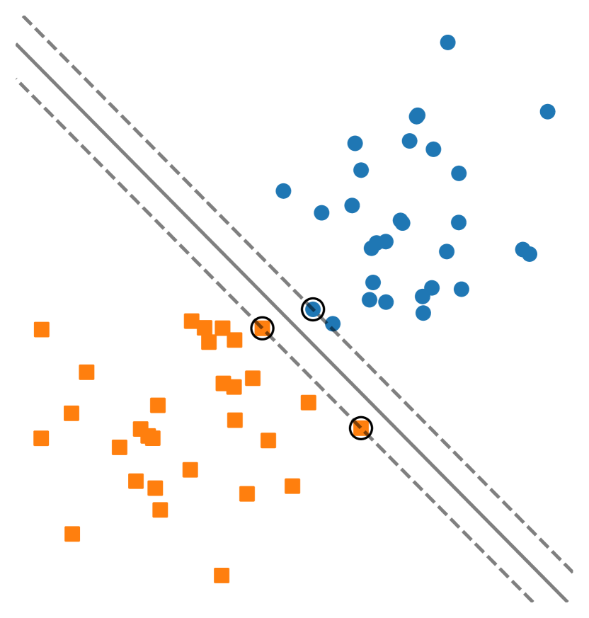
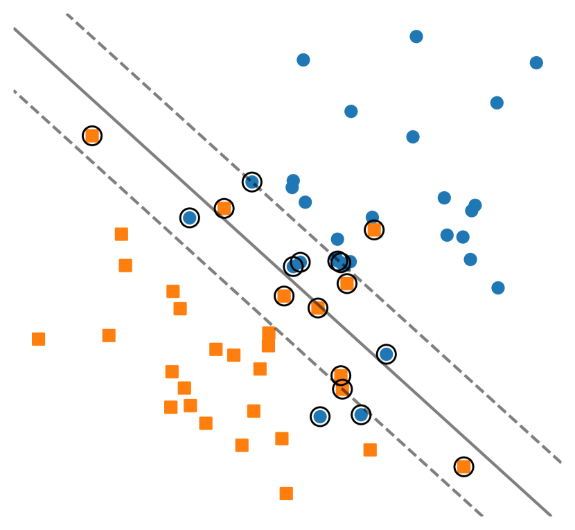
Figure 31: Hard-margin versus soft-margin SVM: Binary classification example: separating orange squares and blue circles with a straight line in the plane. On the left the data is linearly separable, and the solid line is the one separating the squares and circles with maximum margin, i.e., maximizing the minimum distance to the points. The circled points are the closest to the separating line, i.e., these points are the support vectors. On the right, there is no separating straight line, so the dataset is a good candidate for soft-margin SVM, in which the goal is to find a hyperplane that roughly separates the data, and allows some orange squares to be classified as blue circles, and vice-versa. A possible good separator is depicted as a solid line. The circled points are the support vectors, i.e., the points which are either misclassified or lying closer than the margin to the separating line.

We focus in this section on Structural SVMs, which are a generalization of SVMs in which the classification has some structure, arising from a graph or some other combinatorial object [248, 239]. We use the Euclidean norm with the standard scalar product. More formally, given a data point $z\in\mathcal{Z}$ its classification should be from a set $\mathcal{Y}(z)$ depending on the data point itself. A given feature mapping $\phi\colon\mathcal{Z}\times\bigcupop\slimits@_{i=1}^{n}\mathcal{Y}(z_{i})\to\mathbb R^{d}$ maps data points with their possible classifications to a vector space, and the goal is to find a linear classifier $w$, so that a data point $z$ is classified as $\operatorname*{argmax}_{y\in\mathcal{Y}(z)}\mathinner{{}\langle w,\phi(z,y)\rangle}$. To formulate the optimality criterion for $w$, we follow the formulation of [248] and [148]. Given a training dataset $\{z_{i},y_{i}\}_{i=1}^{n}$, i.e., data points $z_{i}$ of class $y_{i}$, we find $w$ by solving

$$\min_{\begin{subarray}{c}\xi_{i}\geq 0\ \forall i\\ \mathinner{{}\langle w,\phi(z_{i},y_{i})\rangle}\geq\mathinner{{}\langle w,\phi(z_{i},y)\rangle}+L(y_{i},y)-\xi_{i}\ \forall i\forall y\in\mathcal{Y}(z_{i})\end{subarray}}\frac{\lambda}{2}\mathinner{{}\lVert w\rVert}_{2}^{2}+\frac{1}{n}\sumop\slimits@_{i=1}^{n}\xi_{i},$$ (244)

where $L(y_{i},y)$ is a loss function returning the penalty for classifying a data point as $y$ when its correct classification is $y_{i}$ (both penalizing incorrect classifications and serving as a soft-margin criterion). This serves as a generalization of the standard zero-one loss, which penalizes all incorrect classifications equally. Note that Problem (244) has $m=\sumop\slimits@_{i=1}^{n}\lvert\mathcal{Y}(z_{i})\rvert$ linear constraints in $w$ and $\xi$, which makes computing a projection, or solving a linear program over the feasible region, computationally prohibitive, because of the potentially huge size of any $\mathcal{Y}(z_{i})$. The unboundedness of the problem is also a disadvantage. These all suggest that a reformulation of Problem (244) should be used instead to eliminate these problems, and the Lagrange dual turns out to be satisfactory:

$$\min_{\begin{subarray}{c}\sumop\slimits@_{y\in\mathcal{Y}(z_{i})}\alpha_{i}(y)=1\ \forall i\\ \alpha\geq 0\end{subarray}}\frac{\lambda}{2}\mathinner{{}\left\lVert\sumop\slimits@_{i=1}^{n}\sumop\slimits@_{y\in\mathcal{Y}(z_{i})}\alpha_{i}(y)\cdot\frac{\phi(z_{i},y_{i})-\phi(z_{i},y)}{\lambda n}\right\rVert}_{2}^{2}\\ +\sumop\slimits@_{i=1}^{n}\sumop\slimits@_{y\in\mathcal{Y}(z_{i})}\frac{L(y_{i},y)}{n}\cdot\alpha_{i}(y),$$ (245)

where $\alpha_{i}(y)$ denotes the dual variable for the constraint $\mathinner{{}\langle w,\phi(z_{i},y_{i})\rangle}\geq\mathinner{{}\langle w,\phi(z_{i},y)\rangle}+L(y_{i},y)-\xi_{i}$ on data point $z_{i}$ and the classification $y\in\mathcal{Y}(z_{i})$. The primal solution is obtained from the dual solution via $w=\sumop\slimits@_{i=1}^{n}\sumop\slimits@_{y\in\mathcal{Y}(z_{i})}\alpha_{i}(y)\cdot\frac{\phi(z_{i},y_{i})-\phi(z_{i},y)}{\lambda n}$.

Note that now Problem (245) has $n$ constraints, and the feasible region is expressed as the Cartesian product of $n$ probability simplices, i.e., each $\alpha_{i}$ lies in a probability simplex. However, there are $m$ dual variables, and this large dimension prevents the use of algorithms that maintain dense representations of the iterates, such as projection-based algorithms for solving the dual problem in Problem (245). On the other hand, we can efficiently use the Frank–Wolfe algorithm, as we can maintain its iterates as convex combinations of vertices of the feasible region, which only have $n$ non-zero elements. Moreover, computing an LMO over the feasible region, expressed as a Cartesian product is trivial.

The algorithm presented in Algorithm 10 [148] solves the dual problem presented in Problem (245) using the vanilla Frank–Wolfe algorithm with line search. The algorithm is termed Primal-Dual because even though it is conceptually solving the dual problem shown in Problem (245), it maintains only the primal solution to avoid having to deal with the $m$ dual variables. For example to compute the gradient note that for some matrices $A$ and $b$, the objective function is $f(\alpha)=\mathinner{{}\lVert A\alpha\rVert}_{2}^{2}+\mathinner{{}\langle b,\alpha\rangle}$ and $w=A\alpha$. The gradient of $f$ is $\nabla f(\alpha)=A^{\top}A\alpha+b=A^{\top}w+b$, and therefore needs only the primal solution $w$. Line 3 minimizes the gradient over the probability simplex of $\alpha_{i}$ by choosing the smallest coordinate of the gradient, making use of the fact mentioned above that the feasible region of the dual problem is the Cartesian product of $n$ probability simplices.

Algorithm 10 Primal-Dual Frank–Wolfe algorithm for structural SVMs [148]

0   Start point $w_{0}=0$, $l_{0}=0$

0   Iterates $w_{0},\dotsc$

1   for $t=0$ to … do

2      for $i=1$ to $n$ do

3          $y_{i}^{*}\leftarrow\operatorname*{argmin}_{y\in\mathcal{Y}(z_{i})}L(y_{i},y)+\mathinner{{}\langle w_{t},\phi(z_{i},y_{i})-\phi(z_{i},y)\rangle}$

4      end for

5      $v_{t}\leftarrow\frac{1}{\lambda n}\sumop\slimits@_{i=1}^{n}\phi(z_{i},y_{i})-\phi(z_{i},y_{i}^{*})$

6      $l\leftarrow\frac{1}{\lambda n}\sumop\slimits@_{i=1}^{n}L(y_{i},y_{i}^{*})$

7      $\gamma_{t}\leftarrow\min\left\{1,\frac{\lambda\mathinner{{}\langle w_{t}-v_{t},w_{t}\rangle}+l_{t}-l}{\lambda\mathinner{{}\lVert w_{t}-v_{t}\rVert}_{2}^{2}}\right\}$

8      $w_{t+1}\leftarrow w_{t}+\gamma_{t}(v_{t}-w_{t})$

9      $l_{t+1}\leftarrow l_{t}+\gamma_{t}(l-l_{t})$

10   end for

More generally, in [148], a block-coordinate generalization of the Frank–Wolfe algorithm is presented, which applies to any problem of the form

$$\min_{x\in\mathcal{M}_{1}\times\dotsm\times\mathcal{M}_{n}}f(x),$$

where $\mathcal{M}_{i}$ is a compact convex set for all $1\leq i\leq n$, and $f$ is a convex function. For example, for the structural SVM dual formulation above in Equation 245 we have $\mathcal{M}_{i}=\{\alpha_{i}\in\mathbb R^{\lvert\mathcal{Y}(z_{i})\rvert}\mid\sumop\slimits@_{y\in\mathcal{Y}(z_{i})}\alpha_{i}(y)=1,\alpha_{i}(y)\geq 0\}$, so $\mathcal{M}_{i}$ is a probability simplex of dimension $\lvert\mathcal{Y}(z_{i})\rvert$. The main idea of the algorithm, shown in Algorithm 11, is to pick one compact convex set $\mathcal{M}_{i}$ uniformly at random at each iteration, and to compute the update for that iteration taking into account only that set. Algorithm 10 above does not use this stochastic update, nevertheless the stochastic update can be used for structural SVMs, too.

We use $[x]_{\mathcal{M}_{i}}$ to denote the set of coordinates of $x$ associated with $\mathcal{M}_{i}$, and $[\nabla f(x)]_{\mathcal{M}_{i}}$ to denote the gradient of $f$ restricted to the coordinates in $\mathcal{M}_{i}$.

Algorithm 11 Block-Coordinate Frank–Wolfe [148]

0   Start point $x_{0}\in\mathcal{M}_{1}\times\dotsm\times\mathcal{M}_{n}$

0   Iterates $x_{1},\dotsc\in\mathcal{M}_{1}\times\dotsm\times\mathcal{M}_{n}$

1   for $t=0$ to … do

2      Pick $i$ uniformly at random from $[1,n]$.

3      $v_{t}\leftarrow\operatorname*{argmin}_{v\in\mathcal{M}_{i}}\mathinner{{}\langle v,[\nabla f(x_{t})]_{\mathcal{M}_{i}}\rangle}$

4      $\gamma_{t}\leftarrow\frac{2n}{t+2n}$

5      $[x_{t+1}]_{\mathcal{M}_{j}}\leftarrow[x_{t}]_{\mathcal{M}_{j}}$ for all $j\neq i$.

6      $[x_{t+1}]_{\mathcal{M}_{i}}\leftarrow(1-\gamma_{t})[x_{t}]_{\mathcal{M}_{i}}+\gamma_{t}v_{t}$

7   end for

Furthermore, one can readily obtain $\mathcal{O}(1/t)$ primal gap and Frank–Wolfe gap convergence guarantees in expectation for these algorithms, shown in Theorem 5.12, using a notion derived from the curvature defined in Section 6.4. With a different problem-specific constant factor, the same convergence holds for variants with a simple, cyclic, deterministic choice of $\mathcal{M}_{i}$ at each iteration, and using the short step rule, see [22].

Theorem 5.12.

Let $f$ be a smooth convex function over $\mathcal{M}_{1}\times\dotsm\times\mathcal{M}_{n}$, a product of compact convex sets $\mathcal{M}_{i}$. Then Algorithm 11 (or a variant with line search) satisfies

$$\mathop{\mathbb{E}}\nolimits\left[f(x_{t})\right]-f(x^{*})\leq\frac{2n}{t+2n}\left(C_{f}^{\otimes}+f(x_{0})-f(x^{*})\right),$$

where $C_{f}^{\otimes}=\sumop\slimits@_{i=1}^{n}C_{f}^{\mathcal{M}_{i}}$, and $C_{f}^{\mathcal{M}_{i}}$ is the curvature of $f$ restricted to the compact convex set $\mathcal{M}_{i}$ (more precisely to $\{[y]_{1}\}\times\dotsm\times\{[y]_{i-1}\}\times\mathcal{M}_{i}\times\{[y]_{i+1}\}\times\dotsm\{[y]_{n}\}$ for any $y$). Moreover, we also have that

$$\mathop{\mathbb{E}}\nolimits\left[\min_{0\leq\tau\leq t}g(x_{\tau})\right]\leq\frac{6n}{t+1}\left(C_{f}^{\otimes}+f(x_{0})-f(x^{*})\right).$$

14.3 The approximate Carathéodory problem

Carathéodory’s theorem is a fundamental result in convex analysis. It states that any point $x$ of an $n$-dimensional convex set $\mathcal{X}$ can be written as a convex combination of at most $n+1$ extreme points of $\mathcal{X}$. This theorem provides the name for the approximate Carathéodory problem: given a polytope $\mathcal{X}$ and a point $u\in\mathcal{X}$, find a point $x\in\mathcal{X}$ which is the convex combination of a small number of distinct vertices $v_{1},\dotsc,v_{k}$ of $\mathcal{X}$ such that $\mathinner{{}\lVert x-u\rVert}\leq\epsilon$. This approximation in the $\ell_{p}$-norm has applications in [18, 19] for computing approximate Nash equilibria and for finding the densest subgraph of a graph. The $\ell_{2}$-ball case has been used to speed up Frank–Wolfe methods in [103] and to find a sparse solution that minimizes the loss of a linear predictor in [229].

Figure 32: Approximate Carathéodory problem in two dimension: approximating a point $u$ of a polygon with convex combinations of at most two vertices, i.e., points on an edge or a diagonal. The point $x$ is the closest approximation in the Euclidean norm.

For $\ell_{2}$-balls, it turns out that one can use the Perceptron algorithm [221] to obtain an approximate solution to the Carathéodory problem [194]. This was later extended to the $\ell_{p}$-norm in [18], $p\geq 2$, with an algorithm that involves finding the exact solution to the convex decomposition, interpreting the convex coefficients as probability distributions and then stochastically sampling from them to find a smaller number of points $v_{1},\ldots,v_{k}$, showing that there exists a point $x$ which is the convex combination of $k=\mathcal{O}(pD_{p}^{2}/\epsilon^{2})$ vertices and such that $\mathinner{{}\lVert x-u\rVert}_{p}\leq\epsilon$, where $D_{p}$ denotes the diameter of $\mathcal{X}$ in the $\ell_{p}$-norm. The method is expensive as we first need to solve the exact problem. More recently, [172] showed that a computationally efficient algorithm based on mirror descent achieved the same result. Furthermore, they proved that $\Omega(pD_{p}^{2}/\epsilon^{2})$ is a lower bound on the number of vertices required to reach $\epsilon$-accuracy in the $\ell_{p}$-norm.

As noted in [172], the mirror descent algorithm solution can be turned into a Frank–Wolfe algorithm solution. The Frank–Wolfe algorithm is particularly well-suited for the approximate Carathéodory problem, as it converges to $u$ by selecting only one vertex at each iteration when applied to the problem $\min_{x\in\mathcal{X}}\mathinner{{}\lVert x-u\rVert}_{p}^{2}$ [69]. We state the convergence result in Theorem 5.13.

Theorem 5.13.

Let $u\in\mathcal{X}$ and $p\geq 2$. Then running the Frank–Wolfe algorithm (Algorithm 1) starting from a vertex $x_{0}\in\mathcal{X}$ with $\gamma_{t}=2/(t+2)$ for minimizing $f(x)=\mathinner{{}\lVert x-u\rVert}_{p}^{2}$ over the polytope $\mathcal{X}$ outputs an iterate $x_{T}$ after $T=\mathcal{O}(pD_{p}^{2}/\epsilon^{2})$ iterations such that

$$\mathinner{{}\left\lVert x_{T}-u\right\rVert}_{p}\leq\epsilon.$$

The iterate $x_{T}$ is the convex combination of at most $T+1$ distinct vertices of $\mathcal{X}$.

Further, improved or new bounds can be derived [69] by applying the convergence rates of FW when $\mathcal{X}$ is strongly convex or when $u\in\operatorname{int}(\mathcal{X})$ (see Table 3), or by applying variants of FW, such as NEP-FW (Algorithm 12) when $u$ lies in the convex hull of a subset of extreme points of $\mathcal{X}$ with small diameter, or HCGS (Algorithm 17) on $\min_{x\in\mathcal{X}}\mathinner{{}\lVert x-u\rVert}_{p}$ when $1\leq p\leq 2$ or $p=+\infty$, which objective is nonsmooth but Lipschitz-continuous.

Example 5.14 (Approximate Carathéodory problem for traffic routing in servers).

We consider a classical example of traffic routing where every device can communicate with only one device at the same time, like in old telephone networks, where switches are set to pair devices for communication, but similar situation also occurs in modern systems, like data centers. Thus a routing is a matching between devices, which changes from time to time to allow single devices communicating with multiple other devices. However, change of routing causes some downtime, so it is desirable to minimize the number of changes. See [60, 92] for more on routing changes, including a more comprehensive setup.

We consider the simplest problem: Find a routing for $n$ senders needing to send some amount of data to $n$ receivers, i.e., matchings between senders and receivers and the amount of time a matching should be used for communication. This amounts to a positive linear decomposition of the matrix $M$ of data to be sent (i.e., sender $i$ needs to send $M_{i,j}$ data to sender $j$) into $0/1$-characteristic matrices of the matchings.

As common in the literature, we restrict to doubly stochastic matrices $M$ in $\mathbb R^{n\times n}$, i.e., that every sender and receiver needs to send the same amount of data altogether. Recall from Example 3.9, that a matrix is doubly stochastic if its entries are nonnegative and its columns and rows sum up to $1$. The problem is then to decompose a given doubly stochastic matrix as a convex combination of permutation matrices, where a sparse decomposition, i.e., one with few permutation matrices is highly desirable. This is an active topic of research [144, see], beneficial for the performance of adaptive server networks [160, 207], as hinted above.

Thus we solve the Carathéodory problem over the Birkhoff␣polytope. By the Birkhoff–von Neumann theorem, any doubly stochastic matrix is the convex combination of at most $(n-1)^{2}+1$ permutation matrices, however, in many cases there are decompositions with much fewer permutation matrices. Finding the minimum number of permutation matrices needed for a convex decomposition is NP-hard [85], and so this motivates attempting to find a convex decomposition that approximates the original matrix in a sparse manner.

In order to test the performance of different Frank–Wolfe variants, we uniformly sample a point $\lambda$ from the probability␣simplex in $\mathbb R^{m}$, and we randomly generate $m=30$ permutation matrices in $\mathbb R^{n\times n}$, denoted by $\{v_{1},\dotsc,v_{m}\}$. We set $u=\sumop\slimits@_{i=1}^{m}\lambda_{i}v_{i}$, and we want to solve $\min_{x\in\mathcal{X}}\mathinner{{}\lVert u-x\rVert}_{2}^{2}$.

We test the performance of several Frank–Wolfe variants that maintain an active set (this rules out variants like the DI-PFW algorithm), more concretely, we compare the performance of the Parameter-free Lazy Conditional Gradient algorithm (LCG, Algorithm 7), the Lazy Away-step Frank–Wolfe algorithm (Lazy AFW, Algorithm 8), the Fully-Corrective Frank–Wolfe algorithm (FCFW, Algorithm 3), the Frank–Wolfe with Nearest Extreme Point Oracle (NEP-FW, Algorithm 12), and the Blended Conditional Gradient algorithm (BCG, Algorithm 15). We use the lazified variants of the CG/FW and the AFW algorithms as they generally obtain sparser solutions than their non-lazified counterparts.

The results are shown in Figure 34 where we show the primal gap when solving the approximate Carathéodory problem, in this case $\mathinner{{}\lVert u-x\rVert}^{2}_{2}$, in the wall-clock time elapsed, and the number of vertices in the convex decomposition of the current iterate. We can observe that given a fixed number of vertices, the FCFW algorithm has a smaller primal gap, or reconstruction error, than the other algorithms in the comparison. However, this comes at a cost, as at each iteration the FCFW algorithm has to minimize the objective function over the convex hull of the current active set, and this can be computationally expensive. The BCG algorithm performs well in this task, as it achieves similar performance to the FCFW algorithm in primal gap versus number of vertices used, but runs faster in wall-clock time than the aforementioned algorithm.

14.4 Video co-localization

The success of many computer vision (CV) applications involving neural networks depends on the quality and the quantity of the labelled data being used to train a given architecture. Manually expanding a dataset by annotating and labelling images is a cumbersome task, which is why there has been a lot of interest in finding efficient ways to label weakly annotated data (i.e., data with some possibly usable extra information (the annotation), where the extra information might be unreliable, be in a free format, or has other usability issues). One such source of data are the videos found on video sharing sites like YouTube or Vimeo. For example, one could be interested in retrieving images of cats from the web to train a neural network. A simple search on YouTube for cat videos reveals a large number of videos that include the word “cat” in the video title, so these videos potentially contain many frames which contain useful cat images. The problem of automatically annotating images of common objects (in this case cats) given the frames of a set of videos is called video co-localization.

We briefly outline at a high level some of the key steps from the realm of CV that allow us to frame this as a tractable optimization problem, as discussed in [136]. We consider a given video to be formed by an ordered series of images. As a first step, for each image of every video, we generate a series of $m$ candidate bounding boxes that contain objects of any kind with well-defined boundaries [5] (as opposed to amorphous background elements). Note that by doing so we might be generating bounding boxes around all kinds of objects like cats, cows, telephone poles, or cars. If we have a total of $n$ images this means that we have a total of $nm$ candidate bounding boxes.

We now want to select one bounding box from each image that contains an object that is common to all the images. In order to do so, we stack the images from each video, from the beginning to the end of each video, and we concatenate the images from different videos together. We now consider a directed graph structure in which the nodes are the bounding boxes in each image. We number these nodes with indices ranging from $1$ to $nm$. We use $\mathcal{I}_{i}$ to denote the set of indices of the nodes obtained from the $i^{th}$ image, with $i\in[1,n]$. The indices of the images refer to the order in which they are stacked, that is, the $i^{th}$ image occurs before the $(i+1)^{st}$ image in the video.

For each image in the stack, we compute a similarity measure between each bounding box and all the bounding boxes in the next image in the stack. We denote this similarity measure between the node $i$ and the node $j$ by $s_{i,j}=s_{j,i}$, with $i\in\mathcal{I}_{k}$ and $j\in\mathcal{I}_{k+1}$ with $k\in[1,n-1]$. If these two nodes are not in temporally adjacent frames, we assign a value of zero for the similarity measure, that is $s_{i,j}=0$ if $i\in\mathcal{I}_{k}$ and $j\notin\mathcal{I}_{k+1}\cap\mathcal{I}_{k-1}$. This similarity measure is based on temporal consistency between the bounding boxes, as we do not expect objects in a box to change drastically in size, position, and form between one frame and the next. If the $s_{i,j}$ is above a given threshold for some $i\in\mathcal{I}_{k}$ and $j\in\mathcal{I}_{k+1}$, we connect the two nodes with a directed edge that points from node $i$ to node $j$. For our simplified example with cats, we have concatenated the frames of two videos together, and we are considering only the first four images of the stacked images, with two bounding boxes each. The resulting graph structure, after computing which nodes to connect based on the temporal similarity measure, is depicted in Figure 33.

Figure 33: The directed graph built from the series of images in a video as a help structure for video colocalization: identifying objects in the video. The nodes in the graph are the bounding boxes of objects in the images. Two nodes are connected if they are in temporally adjacent images/frames, and the bounding boxes satisfy a similarity measure criteria. These are heuristics for connecting bounding boxes of the same object accross the images. In this very simple example, the algorithm creates a series of bounding boxes for each frame and selects two bounding boxes to keep. The algorithm might not create bounding boxes over the same objects in consecutive frames, which is why in the first frame the algorithm creates a bounding box around the cat and around the pole, and in the second frame the algorithm creates a bounding box over the cat and the gutter shown in the image.

Now that we have built a directed graph structure with the bounding boxes, we try to select one (and only one) bounding box in each image so that some similarity criteria is maximized, or respectively some measure of dissimilarity is minimized. This would amount to finding a valid path from the first image in the first video, to the last image in the last video that minimizes some dissimilarity criteria. In order to mathematically frame the problem, we define a variable $z_{i}$ that has a value of $1$ if node $i$ has been selected for output, and $0$ otherwise, and we define a variable $y_{i,j}$ that has a value of $1$ if both node $i$ and the node $j$ have been selected for output. We use $p(k)$ and $c(k)$ to denote the indices of the parent nodes and the child nodes of node $k$. With this structure in mind, we write the following integer optimization problem:

$$\min_{z,y}\quad \mathinner{{}\lVert Uz\rVert}^{2}-\mathinner{{}\langle z,\lambda\rangle}$$ (246)

s.t. $$z_{i}\in\{0,1\},y_{i,j}\in\{0,1\}\quad\forall i,j,$$ (247)

$$\sumop\slimits@_{j\in\mathcal{I}_{i}}z_{j}=1\quad\forall i,$$ (248)

$$\sumop\slimits@_{i\in p(j)}y_{i,j}=\sumop\slimits@_{i\in c(j)}y_{i,j}\quad\forall j\in\mathcal{I}_{k},k\in[2,n-1],$$ (249)

$$y_{i,j}=z_{i}z_{j}\quad\forall i,j.$$ (250)

The convex quadratic objective function $\mathinner{{}\lVert Uz\rVert}^{2}-\mathinner{{}\langle z,\lambda\rangle}$ in this problem measures the dissimilarity criteria for a given set of bounding boxes using temporal and spatial similarity metrics. In Figure 33 this function would measure the dissimilarity between the images in the bounding box $z_{1}$ and $z_{3}$ and $z_{4}$, between $z_{2}$ and $z_{3}$ and so forth. We refer the interested reader to [136] and [237] for the full details of the objective function. Due to the difficulty of solving this integer programming problem over a non-convex set, we instead focus on solving a convex relaxation of the problem presented above, and we minimize the objective function over the convex hull of the non-convex set. The convex hull of the set of constraints shown in Equation (250) is the flow␣polytope. Recalling that the graph has $nm$ vertices, and denoting the number of edges of the graph) by $E$ (i.e., the number of entries of $y$), the complexity of solving the problem in Equation (250), or computing a projection, with an interior point method is $\mathcal{O}((nm)^{3}E+E^{2})$. On the other hand we can solve a linear programming problem with the shortest path problem with complexity $\mathcal{O}(nm+E)$, which motivates the use of Frank–Wolfe algorithms when the number of images and bounding boxes processed is large. In [136], the authors note that the the proposed Frank–Wolfe method for solving the relaxed problem over the convex hull of the non-convex set shown in Equation 250 performs better than several existing algorithms, like the one in [208], for various classes of objects in a well known video-colocalization dataset known as the YouTube-Objects dataset. However, for simple, non-deformable objects, the algorithm in [208] performed better than the proposed Frank–Wolfe-based methodology. The authors in [136] also remark that some algorithms, such as the one presented in [197] outperform the proposed Frank–Wolfe algorithms for all classes in this dataset due to the relatively small size of the dataset, and the fact that the differences among objects in a given class are very large (for example, the different images of aeroplanes in different videos are extremely different, making learning a common aeroplane model difficult).

Approximate Carathéodory	Video Co-localization

Figure 34: Approximate Carathéodory problem for network traffic routing (left) and video co-localization (right): The routing problem formally asks for finding a sparse convex combination of permutation matrices (the vertices) close to a given doubly stochastic matrix $u$. Here we present on the left column the evolution of distance and sparsity (number of vertices in the linear decomposition of current iterate $x_{t}$) in wall-clock time and compared to each other. Distance is the square of the entrywise $\ell_{2}$ norm. In the images on the column on the right we depict the primal gap convergence for the video co-localization problem with the aeroplane dataset presented in [147]. The function being minimized is a convex quadratic function, and the feasible region is the flow polytope.

In the right-side column of Figure 34 we present a comparison of Frank–Wolfe variants when solving a video co-localization problem. The algorithms presented in the comparison are the vanilla FW algorithm (as well as its boosted variant), the AFW algorithm, the DI-PFW algorithm (as well as its boosted variant), and the BCG algorithm. The images and the data used for this example come from the aeroplane image dataset, used in [147] and [136], which leads to a problem with $660$ variables.

For the BoostedFW and the BoostedDI-PFW algorithms we set $\delta=10^{-15}$, and $K=\infty$. For this parameter values we can see in Figure 34 that the BoostDI-PFW algorithm outperforms all other algorithms; it is interesting to observe that is also true for the number of LMO calls, for which the boosting procedure is particularly greedy by nature. All the algorithms are run until the total wall-clock time reaches $600$ seconds, or we reach a solution with a primal gap below $10^{-8}$.

Given that the feasible region is a polytope, more concretely a $0/1$ polytope, and that the objective function is smooth and strongly convex with a condition number of $L/\mu\approx 30$, we expect the AFW, the BCG, and the DI-PFW algorithms to converge linearly in primal gap, in contrast to the FW algorithm, which converges at sublinear rate. This matches with what we observe in the figure that shows the converge in primal gap vs. FOO calls. The BoostedFW, on the hand, can converge in the worst-case at a sublinear rate, like the vanilla FW algorithm, which is what we observe in this experiment. However, in experiments it often converges at a linear rate for this class of problems (see Theorem 3.41. Lastly, the BoostedDI-PFW algorithm exhibits a linear convergence rate for this problem instance, requiring fewer FOO and LMO calls than any of the other algorithms to achieve the final primal gap tolerance. For performance in wall-clock time, we remark that both the DI-PFW and the BoostedDI-PFW algorithms do not require maintenance of an explicit active set, which the BCG and the AFW algorithms require. Operations that involve an active set often scale as $\mathcal{O}(\lvert S\rvert n)$, where $\lvert S\rvert$ is the cardinality of the active set, and $n$ is the dimension of the problem. If the active set grows too large, these operations can quickly become computationally expensive. In the figure that shows the primal gap convergence rate in wall-clock time we can clearly see the difference between the linearly convergent algorithms that do not require an active set (BCG and AFW), and the algorithms that do not require an active set (DI-PFW and BoostedDI-PFW). Moreover, we can also see the difference between the AFW and the BCG algorithms. Not only does the BCG algorithm converge faster than the AFW algorithm in iteration count, but as it maintains an active set of smaller cardinality, it outperforms AFW significantly in wall-clock time. It is important to note however that DI-PFW and BoostedDI-PFW can only be applied to feasible regions that admit a special structure and not to arbitrary polytopes or compact convex sets (see Section 8.1 for a discussion)

14.5 The coreset problem

Many modern applications in machine learning, statistics, and computational geometry rely on using vast amounts of data to train a model, or to compute some estimator or metric. Solving these problems approximately (or exactly, if this is possible at all) typically has complexity that depends on the number of data points used. In many cases, only a small number of data points are relevant or suffice to contain most of the information. This often means that solving the original problem over this smaller dataset yields approximately the same result as using the original dataset, while being cheaper to compute.

For simplicity of exposition, we consider a similar, simply formulated geometric problem here: the Minimum Enclosing Ball (MEB) problem, from computational geometry, which is to find the ball $B(c_{\mathcal{S}},r_{\mathcal{S}})$ of minimum radius $r_{\mathcal{S}}>0$ containing a given set $\mathcal{S}$ of $m$ points in $\mathbb R^{n}$, where $c_{\mathcal{S}}$ and $r_{\mathcal{S}}$ denote the center and the radius of the MEB of $\mathcal{S}$, respectively. Computing the MEB of $\mathcal{S}$ can be done exactly with a randomized algorithm with expected complexity $\mathcal{O}(m(n+2)!)$ [258]. Note that the factorial complexity in the dimension $n$ makes the algorithm impractical for large dimensions. One question that arises is: if we find the MEB of $\mathcal{S}^{\prime}$, a subset of $\mathcal{S}$, will it be a good approximation (where we have yet to define what “good” is) to the MEB of $\mathcal{S}$? That is, can we solve a cheaper problem with fewer points to obtain a “good-enough” solution?

This is the intuition behind the coreset problem. Many different definitions of an $\epsilon$-coreset for the MEB problem have arisen in the literature. At first, an $\epsilon$-coreset with $\epsilon>0$ of $\mathcal{S}$ for the MEB problem was defined as a set $\mathcal{S}^{\prime}\subseteq\mathcal{S}$ such that MEB $B(c_{\mathcal{S}^{\prime}},r_{\mathcal{S}^{\prime}})$ of $\mathcal{S}^{\prime}$ scaled by $1+\epsilon$, i.e., the ball $B(c_{\mathcal{S}^{\prime}},(1+\epsilon)r_{\mathcal{S}^{\prime}})$ contains the MEB of $\mathcal{S}$ [14]. However, in this section we focus on the broader definition from [65], recalled as Definition 5.15 below (which is closely related to the one in [265]). A subset $\mathcal{S}^{\prime}\subseteq\mathcal{S}$ is an $\epsilon$-coreset for $\mathcal{S}$ if $r_{\mathcal{S}}^{2}\leq r_{\mathcal{S}^{\prime}}^{2}/(1-2\epsilon)$. Note that since $c_{\mathcal{S}}\in\operatorname{conv}(\mathcal{S})$ by Carathéodory’s theorem there always exists a $0$-coreset of at most $n+1$ points for the MEB problem, where $n$ is the dimension of the space containing $S$ (i.e., $S\subseteq\mathbb{R}^{n}$).

The concept of coreset problem can be applied to a wide variety of scenarios, which all share a common form, and which is suited to the application of Frank–Wolfe algorithms [65] (this expands and sharpens the analysis of the coreset problem [14]). Many of these problems, like MEB, can be phrased as a concave maximization problem:

$$\max_{x\in{}_{m}}f(x),$$ (251)

where $f\colon\mathbb{R}^{m}\to\mathbb{R}$ is a concave differentiable function and ${}_{m}=\{x\in\mathbb{R}^{m}\mid x^{\top}\mathds{1}=1,x\geq 0\}$ is the probability␣simplex. For example, given a set of points $\mathcal{S}=\{a_{1},\dotsc,a_{m}\}$ in $\mathbb R^{n}$, the MEB problem can be phrased as:

$$\min_{c\in\mathbb{R}^{n},r>0}\quad r^{2}$$ (252)

s.t. $$\mathinner{{}\lVert a_{i}-c\rVert}_{2}^{2}\leq r^{2}\quad\forall 1\leq i\leq m$$ (253)

Taking the Lagrange dual leads to

$$\max_{x\in{}_{m}}\underbrace{\sumop\slimits@_{i=1}^{m}x_{i}\mathinner{{}\lVert a_{i}\rVert}_{2}^{2}-\mathinner{{}\left\lVert\sumop\slimits@_{i=1}^{m}x_{i}a_{i}\right\rVert}_{2}^{2}}_{f(x)}.$$ (254)

Thus the dual problem of the MEB problem has the form shown in Equation (251). The primal problem satisfies Slater’s condition (take any $c\in\operatorname{conv}(\mathcal{S})$ and a large enough $r$), and thus strong duality holds, therefore let $x^{*}\in\operatorname*{argmax}_{x\in{}_{m}}f(x)$, then one recovers the MEB for $\mathcal{S}$ via $c_{\mathcal{S}}=\sumop\slimits@_{i=1}^{m}x_{i}^{*}a_{i}$ and $r_{\mathcal{S}}^{2}=f(x^{*})$. Note that Equation (251) is a maximization problem, and the primal gap and Frank–Wolfe gap at $x$ are given by $f(x^{*})-f(x)$, and $g(x)=\max_{v\in{}_{m}}\mathinner{{}\langle\nabla f(x),v-x\rangle}=\max_{1\leq i\leq m}\nabla f(x)_{i}-\mathinner{{}\langle\nabla f(x),x\rangle}$, respectively.

For any $\mathcal{N}\subseteq\{1,2,\dotsc,m\}$, let ${}^{\mathcal{N}}\stackrel{{\scriptstyle\textnormal{\scriptsize def}}}{{=}}\operatorname{conv}(e_{i}\mid i\in\mathcal{N})$, where the $e_{i}$ are the coordinate vectors, and let $x^{\mathcal{N}}\in\operatorname*{argmax}_{x\in{}^{\mathcal{N}}}f(x)$ for any $\mathcal{N}\subseteq\{1,2,\dotsc,m\}$. Before formally defining a coreset, we first recall a local version of the curvature $C$ presented in Section 6.4:

$$C_{f}^{*}\stackrel{{\scriptstyle\textnormal{\scriptsize def}}}{{=}}\sup_{\begin{subarray}{c}z\in{}_{m}\\ \alpha\in\mathbb{R}\\ y=x^{*}+\alpha(z-x^{*})\in{}_{m}\end{subarray}}\frac{1}{\alpha^{2}}\bigl{(}f(x^{*})-f(y)+\mathinner{{}\langle\nabla f(x^{*}),y-x^{*}\rangle}\bigr{)}\geq 0.$$

With this in mind:

Definition 5.15.

Given a concave function $f(x)$, and $\epsilon>0$, an $\epsilon$-coreset for Problem (251) is a subset $\mathcal{N}\subseteq\{1,2,\dotsc,m\}$ satisfying $f(x^{*})-f(x^{\mathcal{N}})\leq 2\epsilon C_{f}^{*}$.

Looking at Definition 5.15, one can quickly see that returning an $0$-coreset is trivial, simply return $\mathcal{N}=\{1,2,\dotsc,m\}$. However, this solution is of no use, as in most problems the whole point of a coreset is finding a set $\mathcal{N}$ of cardinality much smaller than $m$ such that computing $x^{\mathcal{N}}\in\operatorname*{argmax}_{x\in{}^{\mathcal{N}}}f(x)$ is much cheaper than computing $x^{*}$ by solving Problem (251), while ensuring that the solution found using $\mathcal{N}$ satisfies $f(x^{*})-f(x^{\mathcal{N}})\leq 2\epsilon C_{f}^{*}$.

Remark 5.16.

The definition of a $\epsilon$-coreset in Definition 5.15 is different than the one presented in [65], where an $\epsilon$-coreset is defined as a subset $\mathcal{N}$ satisfying $g(x^{\mathcal{N}})\leq 2\epsilon C_{f}^{*}$, where $g(x)$ denotes the Frank–Wolfe gap at $x$ for Problem (251). It is important to state that both definitions qualitatively try to characterize what are good subsets $\mathcal{N}$ that will provide a “good-enough” solution to the original problem. However, there are two reasons why we use Definition 5.15, as opposed to the definition in [65].

First, note that a point $x$ encoded by a subset $\mathcal{N}$, such that $f(x^{*})-f(x)\leq 2\epsilon C_{f}^{*}$, encodes an $\epsilon$-coreset according to Definition 5.15, as $f(x)\leq f(x^{\mathcal{N}})$. From a practical point of view, if we find a point such that $g\left(x\right)\leq 2\epsilon C_{f}^{*}$, this point certifiably encodes an $\epsilon$-coreset according to Definition 5.15, as $f(x^{*})-f(x)\leq g(x)$, and we do not even need to find $x^{\mathcal{N}}\in\operatorname*{argmax}_{x\in{}^{\mathcal{N}}}f(x)$ in order to show that $\mathcal{N}$ is an $\epsilon$-coreset according to Definition 5.15. However, according to the definition of [65], a point that satisfies $g\left(x\right)\leq 2\epsilon C_{f}^{*}$ is not an $\epsilon$-coreset, as there is no way to certify that $g(x^{\mathcal{N}})\leq 2\epsilon C_{f}^{*}$ other than solving $x^{\mathcal{N}}\in\operatorname*{argmax}_{x\in{}^{\mathcal{N}}}f(x)$ and computing its Frank–Wolfe gap. This is due to the fact that even though $g(x)\leq 2\epsilon C_{f}^{*}$, it is possible that $g(x^{\mathcal{N}})>2\epsilon C_{f}^{*}$, despite the fact that the $\mathcal{N}$ determined by $x$ such that $g(x)\leq 2\epsilon C_{f}^{*}$ would allow us to obtain a good solution to the problem in Equation 251.

Secondly, using Definition 5.15 allows us to analyse in a more direct fashion the algorithms presented later on in this section, as most of the convergence rates presented in this survey are primal gap convergence rates, and quantifying the number of iterations $t$ until $f(x^{*})-f(x_{t})\leq 2\epsilon C_{f}^{*}$ becomes straightforward (as opposed to quantifying the number of iterations until $g(x^{\mathcal{N}_{t}})\leq 2\epsilon C_{f}^{*}$).

Remark 5.17.

Returning to the case of the MEB problem, if we are given a set of points $\mathcal{S}=\{a_{1},\cdots,a_{m}\}$, and we note that, $f(x^{*})=r^{2}_{\mathcal{S}}$, then an $\epsilon$-coreset encodes a set of points $\mathcal{S}^{\prime}=\{a_{i}\mid i\in\mathcal{N}\}$ through $\mathcal{N}$, such that $r^{2}_{\mathcal{S}}-r^{2}_{\mathcal{S}^{\prime}}\leq 2\epsilon C_{f}^{*}$. That is, a coreset gives us a smaller set of points that give us a solution that is $\epsilon$-“good-enough” compared to the solution to the original MEB problem. To see this more clearly, note that for the case of the MEB, problem, we have that

$$C_{f}^{*}=\sup_{\begin{subarray}{c}z\in{}_{m}\\ \alpha\in\mathbb{R}\\ y=x^{*}+\alpha(z-x^{*})\in{}_{m}\end{subarray}}\frac{1}{\alpha^{2}}\mathinner{{}\left\lVert\sumop\slimits@_{i=1}^{m}a_{i}y_{i}-c_{\mathcal{S}}\right\rVert}_{2}^{2}=r_{\mathcal{S}}^{2}.$$ (255)

This means that solving the MEB problem over a $2\epsilon C_{f}^{*}$-coreset yields a $r^{2}_{\mathcal{S}^{\prime}}$ such that $r^{2}_{\mathcal{S}}\leq r^{2}_{\mathcal{S}^{\prime}}/(1-2\epsilon)$.

Due to the fact that the Frank–Wolfe algorithm accesses at most one vertex of the probability simplex at each iteration, it has been successfully applied to the coreset problem (see Algorithm 12, which is nothing but the vanilla FW algorithm with line search applied to the maximization problem in Problem (251), and run until the Frank–Wolfe gap is below $\epsilon$), and has been used to characterize the cardinality of the set $\mathcal{N}$ that can allow us to reach a given $\epsilon$-coreset for a given problem.

Algorithm 12 Frank–Wolfe for the coreset problem [65]

0   Initial point $x_{0}=\operatorname*{argmax}_{1\leq i\leq m}f(e_{i})$, index set $\mathcal{N}_{0}=\{x_{0}\}$, and accuracy $\epsilon>0$

0   Subset $\mathcal{N}_{t}\subseteq\{1,2,\dotsc,m\}$ and solution $x_{t}\in\mathcal{S}^{\mathcal{N}_{t}}$

1   for $t=0$ to … do

2      $i_{t}\leftarrow\operatorname*{argmax}_{1\leq i\leq m}[\nabla f(x_{t})]_{i}$

3      $\gamma_{t}\leftarrow\operatorname*{argmax}_{\gamma\in\mathbb R}f(x_{t}+\gamma(e_{i_{t}}-x_{t}))$

4      $x_{t+1}\leftarrow x_{t}+\gamma_{t}(e_{i_{t}}-x_{t})$

5      $\mathcal{N}_{t+1}\leftarrow\mathcal{N}_{t}\cup\{i_{t}\}$

6      $t\leftarrow t+1$

7   end for

Theorem 5.18.

Given a concave function $f$, the vanilla Frank–Wolfe algorithm with line search (Algorithm 12) returns a $2\epsilon C/C_{f}^{*}$-coreset in $t=\mathcal{O}(1/\epsilon)$ iterations, resulting in a coreset $\mathcal{N}_{t}$ of cardinality at most $t$.

Thus the coreset problem attempts to balance the cardinality of $\mathcal{N}_{t}$ with the accuracy one can expect to achieve with $\mathcal{N}_{t}$. The way in which the balance tips towards one side or the other depends on the application at hand. As a rule of thumb, if computing $x^{\mathcal{N}_{t}}$ depends very unfavourably on the cardinality of $\mathcal{N}_{t}$, one will settle for coarser, or less accurate solutions, to the coreset problem. If on the other hand, computing $x^{\mathcal{N}_{t}}$ is expensive, but manageable, we will tip towards finer, or more accurate solutions to the coreset problem. We will see in Example 5.19, that for the MEB problem in $\mathbb R^{3}$, one can often find coreset of points of cardinality around $10$ that allows us to compute an MEB solution that is extremely close to the solution to the MEB problem using around $500,000$ points.

To obtain coresets of smaller cardinality [65] essentially proposed to use the Fully-Corrective Frank–Wolfe algorithm. The convergence rate of this algorithm for the coreset problem is the same as the one shown for the vanilla Frank–Wolfe algorithm with line search. One can also blend the steps taken by the FCFW algorithm with those taken by the AFW algorithm obtaining an Away-step/Fully-Corrective Frank–Wolfe blend for the coreset problem [15].

Example 5.19 (Coreset for the MEB problem).

We showcase the performance of the different Frank–Wolfe variants for the coreset problem with an MEB application. As stated before, at a high level, this problem aims to find the ball with the smallest volume that encloses a given set of points. We use two different sets of points in $\mathbb R^{3}$ for this application, which are commonly used in computer graphics, namely, the Stanford bunny [250], and the Stanford dragon [72], which have $35,947$ and $566,098$ points respectively. For example, the MEB problem has been used for fast collision detection, in which one has to detect in a time-critical manner if a collision between two objects has occurred, or is about to occur [128]. In this case, each object (typically represented as a large set of vertices) is approximated by a collection of a few balls that contain these vertices. These balls are used to approximately detect in a fast manner if a collision between these two objects has occurred or is about to occur, as it is typically computationally easier to check if a small set of balls intersects with another small set of balls, than to check if two polyhedra with a large number of vertices intersect.

Figure 35: Set of points for the coreset MEB (minimal enclosing ball) experiment, here forming bodies in $3$ dimension: the Stanford bunny ($35{,}947$ points) on the left, and the Stanford dragon ($566{,}098$) on the right.

Computing the MEB of a series of $m$ points in $\mathbb R^{n}$ can be done exactly with Welzl’s algorithm (with expected complexity $\mathcal{O}(m(n+1)(n+1)!)$ [258]). For the Stanford bunny (with $m=35,947$ points), it takes approximately $630$ seconds to compute the MEB using all the data points (which both have a MEB or radius approximately $0.1$ meters), using the implementation of Welzl’s package in the miniball package. For the Stanford dragon, we were not able to run the aforementioned implementation of Welzl’s algorithm as it exceeded the memory limit of the machine being used. Note that we have not used faster (and more efficient) packages based on Cython/Python bindings to Welzl’s algorithm in C++ to provide a fair comparison to the rest of the code, which is based exclusively in Python, and have therefore used a MEB implementation fully written in Python. For full transparency, using the cyminiball package, with Cython/Python bindings to C++, one can solve the MEB problem for the Stanford dragon in $0.5$ seconds with a low memory footprint.

Stanford bunny	Stanford dragon

Figure 36: Coreset MEB (minimal enclosing ball): Performance of Frank–Wolfe algorithms for finding coresets of the Standford animals (see Figure 35). The figures show the per iteration progress: the first row depicts an upper bound $f(x^{*})-f(x_{t})$ on the accuracy of the current coreset $\mathcal{N}_{t}$ obtained from the current iterate $x_{t}$ with minimal computation, the second row depicts the true accuracy $f(x^{*})-f(x^{\mathcal{N}_{t}})$ of the coreset, and the third row depicts the size $\lvert\mathcal{N}_{t}\rvert$ of the current coreset. (The objective function $f$ is the concave function from Equation (254).) The second shows FCFW quickly identifying a very good coreset in a few iterations, at the cost of these iterations being more computationally expensive than for the other algorithms.

In the left column of Figure 36 we see the performance of the FW algorithm (Algorithm 12), the AFW algorithm (Algorithm 2), and the FCFW algorithm (Algorithm 3) on the coreset problem for the MEB setting using the data from the Stanford bunny. It is important to remark that all the algorithms identify a coreset in less than $10$ iterations with which one can obtain a high accuracy solution to the MEB problem with the full dataset. The cardinality of this coreset is $8$ for the FW algorithm, around 3–5 for the AFW algorithm, and $6$ for the FCFW algorithm. The FCFW algorithm identified the appropriate coreset, and obtained a high accuracy solution to the MEB problem with Welzl’s algorithm in less than a second, compared to the $630$ seconds it took to compute the MEB with the full set of $35{,}947$ points.

In the right column of Figure 36 we see the performance of the algorithms mentioned in the previous paragraph using the the data from the Stanford dragon. Again, all the algorithms identify a coreset in less than $10$ iterations obtaining a high accuracy solution to the MEB problem with the full dataset (which has $566{,}098$ points in total).

14.6 Adversarial attacks

Given a (trained) model, adversarial machine learning consists of finding input data points for which the model predicts deceptive labels, the end goal being to check the robustness of the model. In other words, a model is an algorithm with a data point as input and a label as output. In this context, the role of the adversary is to find a data point $x$ that is $\epsilon$-close to a data point $\hat{x}$ with label $\hat{y}$ and for which the model predicts a label $y\neq\hat{y}$ (Figure 37). More precisely, the adversary can specify the label $y\neq\hat{y}$ and search for a data point $x$ such that $\mathinner{{}\lVert x-\hat{x}\rVert}_{p}\leq\epsilon$. The distance between $x$ and $\hat{x}$ is usually measured in the $\ell_{p}$-norm, $p\geq 1$, the $\ell_{\infty}$-norm being particularly often used in the literature on adversarial learning. The problem can be formulated as follows:

$$\min_{\mathinner{{}\lVert x-\hat{x}\rVert}_{p}\leq\epsilon}\ell(x,y),$$

where $\ell(x,y)$ is a classification loss function.

original image: daisy	perturbation $\epsilon=0.03$	adversarial image: quill pen

Figure 37: Schematic of an adversarial attack in computer vision: An image classifying algorithm, here a trained neural network, is fooled by minor differences undetectable to the human eye: it correctly classifies the left image as “daisy”, while it classifies the right image as “quill pen”. The right image has been obtained by adding some low yet carefully selected noise to the left image, which humans don’t perceive. While this example is benign and funny, implications can be much more harmful: what if a self-driving car classifies a stop sign for a speed limit, simply because there was a tiny stain on it? The example here is from the NIPS2017 dataset.

There are two settings to be considered: the white-box setting, where the adversary has complete access to the model, e.g., for a neural network model, access to the architecture and the weights, and the black-box setting, where the adversary has access only to the inputs and outputs of the model. In practice, the difference between white-box and black-box attacks is that the adversary cannot perform backpropagation to compute the gradient of the loss function $\ell$. Thus, [59] use the classical Frank–Wolfe variant with momentum in the white-box setting and a zeroth-order variant with momentum in the black-box setting. The motivation for using the Frank–Wolfe algorithm here is that the iterates of projection-based attacks will likely be on the boundary of the $\ell_{p}$-ball very fast, while the iterates of Frank–Wolfe tend to remain in the interior of the ball. Thus, the distortion $\mathinner{{}\lVert x-\hat{x}\rVert}_{p}$ will likely be lower, hence better, by using the Frank–Wolfe algorithm. Furthermore, linear minimizations over $\ell_{p}$-balls have closed-form solutions while projections can be very expensive when $p\neq 1,2,+\infty$, as already stated in Table 1.

In both settings, the Frank–Wolfe algorithm converges at a rate $\min_{1\leq t\leq T}g_{t}=\mathcal{O}(1/\sqrt{T})$ and $\mathbb{E}[\min_{1\leq t\leq T}g_{t}]=\mathcal{O}(1/\sqrt{T})$, where $T$ is the total number of iterations (fixed in advance). These have been compared to FGSM [113], PGD [166], and MI-FGSM [80] in the white-box setting, and to NES-PGD [129] and bandit attack [130] in the black-box setting, where the goal is to attack the MNIST [153] and ImageNet [75] datasets. Computational experiments show that among these methods, the Frank–Wolfe approach yields the best attack success rates (together with PGD and MI-FGSM in the white-box setting), and with the fastest convergence and the lowest distortion.

Adversarial training has the goal is to train a neural network with defence against adversarial attacks, e.g, by using a robust optimization formulation. [166] analyze distortions in the $\ell_{2}$-norm and $\ell_{\infty}$-norm caused by training via projected gradient descent and demonstrate strong resistance to gradient obfuscation. Adversarial training using Frank–Wolfe was then proposed in [247].

Another defence is the use of interpretable neural networks, which provide brief explanation for their predictions. The intent of the explanation is independent verification of the predictions, e.g., by humans. Defence against adversarial attacks is a by-product, as the goal usually is to detect wrong prediction for naturally occurring real-world data. See [165] for the use of conditional gradients in interpretable neural networks.

14.7 Optimal experimental design

In physics, biology, and medicine many experiments are expensive or time consuming, so that minimizing the number of experimental runs or sample sizes is desirable. Therefore there is a need for optimal designs, i.e., designs of experiments optimal for some statistical criterion.

In this section, we consider a simple example, where we want to learn $x^{*}\in\mathbb{R}^{d}$, but we can only measure some linear function of it that has been contaminated by Gaussian noise, i.e., we can observe $y=\mathinner{{}\langle a,x^{*}\rangle}+\omega$ where $\omega$ is a normally distributed random variable with zero mean and variance $\sigma^{2}$. We further assume that the measurement vector $a$ can be chosen only among finitely many values: $a_{1},\dotsc,a_{n}$, which generate the vector space $\mathbb{R}^{d}$. The goal is to find the numbers of times $m_{1},\dotsc,m_{n}$ we must repeat the measurement for each $a_{1},\dotsc,a_{n}$ in order to satisfy some statistical criterion. We assume that we can perform a very large, fixed total number $m\stackrel{{\scriptstyle\textnormal{\scriptsize def}}}{{=}}\sumop\slimits@_{i=1}^{n}m_{i}$ of measurements.

Let $V([x]_{1},\dotsc,[x]_{n})\stackrel{{\scriptstyle\textnormal{\scriptsize def}}}{{=}}\sumop\slimits@_{i=1}^{n}[x]_{i}a_{i}a_{i}^{\top}$. As is well-known, the least-squares unbiased estimator for $x^{*}$ is

$$\hat{x}\stackrel{{\scriptstyle\textnormal{\scriptsize def}}}{{=}}\sumop\slimits@_{j=1}^{m}y_{j}V(m_{1},\dotsc,m_{n})^{-1}a_{i_{j}},$$

where $a_{i_{j}}$ is the measurement vector chosen for the $j$-th measurement and $y_{j}$ is a random realization of $\mathinner{{}\langle a_{i_{j}},x^{*}\rangle}+\omega$. The estimator $x^{*}$ is normally distributed with mean $x^{*}$ and covariance matrix $\sigma^{2}V(m_{1},\dotsc,m_{n})^{-1}$.

There are many optimization criteria for optimal experiment design, of which we consider only D-optimal design, which maximizes the information content about $x^{*}$ of the estimate $\hat{x}$, as measured by the differential Shannon entropy. This boils down to maximizing $\det V(m_{1},\dotsc,m_{n})$. For ease of exposition we focus on the continuous (approximate) design of experiments where the $m_{i}$ can take any positive real value, assuming the total number of experiments $m$ is large enough so that rounding introduces minimal error. Reparametrizing with $[x]_{i}\stackrel{{\scriptstyle\textnormal{\scriptsize def}}}{{=}}m_{i}/m$, the goal becomes that of maximizing $\det V(m_{1},\dotsc,m_{n})=m^{d}\det V([x]_{1},\dotsc,[x]_{n})=m^{d}V(x)$ with $x\stackrel{{\scriptstyle\textnormal{\scriptsize def}}}{{=}}([x]_{1},\dotsc,[x]_{n})$ lying in the probability␣simplex ${}_{n}\stackrel{{\scriptstyle\textnormal{\scriptsize def}}}{{=}}\{x\mid\sumop\slimits@_{i=1}^{n}[x]_{i}=1,x\geq 0\}$. We write $[x]_{i}$ for the coordinate $i$ of $x$ to distinguish it from the iterate $x_{i}$ of the algorithm below and we choose an equivalent objective function, which is convex, so that the optimization problem becomes

$$\min_{x\in{}_{n}}\bigl{(}-\ln\det V(x)\bigr{)}\qquad f(x)\stackrel{{\scriptstyle\textnormal{\scriptsize def}}}{{=}}-\ln\det V(x).$$ (256)

Note that the objective function shown in Problem (256) has a Lipschitz continuous gradient for points on the relative interior of _n. As a side remark, the dual of the problem shown in Equation 256 has a geometric interpretation: it is the minimum volume enclosing ellipsoid problem, in which we want to find the ellipsoid with the smallest volume that contains $a_{1},\dotsc,a_{n}$ [234]. See [152, Chapter 21 ] for connections to bandit algorithms.

Recall that $\ln\det V$ is a concave function in $V$ for $V$ positive definite, and its gradient is given via

$$\mathinner{{}\langle\nabla\ln\det V,X\rangle}=\operatorname{Tr}\left[{V^{-1}X}\right].$$

In particular, this provides the scalar product of the gradient of the objective function with the vertices of _n, i.e., with the coordinate vectors $e_{1},\dotsc,e_{n}$:

$$\begin{split}\mathinner{{}\langle\nabla f(x),e_{i}\rangle}=\frac{\partial f(x)}{\partial[x]_{i}}&=-\operatorname{Tr}\left[{V(x)^{-1}\frac{\partial V(x)}{\partial[x]_{i}}}\right]=-\operatorname{Tr}\left[{V(x)^{-1}a_{i}a_{i}^{\top}}\right]\\ &=-a_{i}^{\top}V(x)^{-1}a_{i}=-\mathinner{{}\lVert a_{i}\rVert}_{V(x)^{-1}}^{2}\end{split}$$

Now the vanilla Frank–Wolfe algorithm (Algorithm 1) with exact line search for the D-optimal design Problem (256) becomes Algorithm 13 [94, which was originally proposed by], with Line 2 computing the index of the Frank–Wolfe vertex.

Algorithm 13 Frank–Wolfe for D-optimal design [94]

0   Start point $x\in{}_{n}$, measurement vectors $a_{1},\dotsc,a_{n}$

0   Iterates $x_{1},\dotsc$

1   for $t=0$ to … do

2       $i_{t}\leftarrow\operatorname*{argmax}_{1\leq i\leq n}\mathinner{{}\lVert a_{i}\rVert}_{V(x_{t})^{-1}}^{2}$

3       $\gamma_{t}\leftarrow\frac{(1/n)\mathinner{{}\lVert a_{i_{t}}\rVert}_{V(x_{t})^{-1}}^{2}-1}{\mathinner{{}\lVert a_{i_{t}}\rVert}_{V(x_{t})^{-1}}^{2}-1}$

4      $x_{t+1}\leftarrow(1-\gamma_{t})x_{t}+\gamma_{t}e_{i_{t}}$ {$e_{i}$ is coordinate vector $i$.}

5   end for

Line 3 is actually the closed form solution to line search. We include a proof for completeness. We compute the derivative of the objective function in $\gamma$ when moving from $x_{t}$ to $x_{t}+\gamma(e_{i_{t}}-x_{t})$ via simple manipulations and the Sherman–Morrison formula:

$$\begin{split}&\frac{\partial f\bigl{(}x_{t}+\gamma(e_{i_{t}}-x_{t})\bigr{)}}{\partial\gamma}\\ &=-\operatorname{Tr}\left[{V(x_{t}+\gamma(e_{i_{t}}-x_{t}))^{-1}\frac{\partial V\bigl{(}x_{t}+\gamma(e_{i_{t}}-x_{t})\bigr{)}}{\partial\gamma}}\right]\\ &=-\operatorname{Tr}\left[{[V(x_{t})(1-\gamma)+\gamma a_{i_{t}}a_{i_{t}}^{\top}]^{-1}\bigl{(}a_{i_{t}}a_{i_{t}}^{\top}-V(x_{t})\bigr{)}}\right]\\ &=-\operatorname{Tr}\left[{\left(\frac{V(x_{t})^{-1}}{(1-\gamma)}-\frac{\gamma}{(1-\gamma)^{2}}\frac{V(x_{t})^{-1}a_{i_{t}}a_{i_{t}}^{\top}V(x_{t})^{-1}}{1+\gamma a_{i_{t}}^{\top}V(x_{t})^{-1}a_{i_{t}}/(1-\gamma)}\right)\bigl{(}a_{i_{t}}a_{i_{t}}^{\top}-V(x_{t})\bigr{)}}\right]\\ &=\frac{1}{1-\gamma}\left(n-\mathinner{{}\lVert a_{i_{t}}\rVert}_{V(x_{t})^{-1}}^{2}+\frac{\gamma\mathinner{{}\lVert a_{i_{t}}\rVert}_{V(x_{t})^{-1}}^{2}(\mathinner{{}\lVert a_{i_{t}}\rVert}_{V(x_{t})^{-1}}^{2}-1)}{1-\gamma+\gamma\mathinner{{}\lVert a_{i_{t}}\rVert}_{V(x_{t})^{-1}}^{2}}\right).\end{split}$$

The minimal function value occurs at the zero of the derivative, i.e., at $\gamma=[(1/n)\mathinner{{}\lVert a_{i_{t}}\rVert}_{V(x_{t})^{-1}}^{2}-1]/(\mathinner{{}\lVert a_{i_{t}}\rVert}_{V(x_{t})^{-1}}^{2}-1)$.

The fact that there is a closed form expression for the line search already shows that this algorithm has the advantage of having to perform cheaper basic operations than other algorithms, due to the fact that the algorithm only moves towards vertices of _n. Note that no closed form expression is known for the line search between two arbitrary points on the simplex for $f$, which is a disadvantage e.g., for projected gradient descent. The following recursive formulae provide further optimization possibilities: implementing each matrix operation (like computing the determinant and the inverse of a matrix) in Algorithm 13 can be done using only $\mathcal{O}(d^{2})$ arithmetic operations. However, in the first iteration we still have to compute $V(x_{0})^{-1}$ and $\det V(x_{0})$ with $\mathcal{O}(d^{3})$ arithmetic operations. The recursive nature of the formulae accumulates computational errors across iterations, so periodically computing the quantities directly is still advisable in practice.

$$\begin{split}\det V(x_{t+1})&=(1-\gamma_{t}+\gamma_{t}\mathinner{{}\lVert a_{i_{t}}\rVert}_{V(x_{t})^{-1}}^{2})(1-\gamma_{t})^{d-1}\det V(x_{t}),\\ V(x_{t+1})^{-1}&=\frac{1}{1-\gamma_{t}}\left(V(x_{t})^{-1}-\frac{\gamma_{t}V(x_{t})^{-1}a_{i_{t}}a_{i_{t}}^{\top}V(x_{t})^{-1}}{1-\gamma_{t}+\gamma_{t}\mathinner{{}\lVert a_{i_{t}}\rVert}_{V(x_{t})^{-1}}^{2}}\right).\intertext{For the gradient of $f$, the following formulae needs only $\mathcal{O}(d)$ arithmetic operations (essentially the scalar product with $a_{i}$) per coordinate:}\mathinner{{}\langle\nabla f(x_{t+1}),e_{i}\rangle}&=\frac{1}{1-\gamma_{t}}\left(\mathinner{{}\langle\nabla f(x_{t}),e_{i}\rangle}-\frac{\gamma_{t}(a_{i}^{\top}V(x_{t})^{-1}a_{i_{t}})^{2}}{1-\gamma_{t}+\gamma_{t}\mathinner{{}\lVert a_{i_{t}}\rVert}_{V(x_{t})^{-1}}^{2}}\right).\end{split}$$

Finally, we note that Algorithm 13 has an away-step version relying on the Away-Step Frank–Wolfe algorithm (Algorithm 2) instead of the vanilla Frank–Wolfe algorithm. Note that as the away steps of the aforementioned algorithm move away from the vertices of _n, the optimizations shown above also apply, e.g., there is a similar closed-form solution for the line search for away steps. Also, for both algorithms, if $x_{0}=\mathds{1}/n$ with $n>1$ and the non-zero vectors $a_{1},\dotsc,a_{n}$ generate the vector space $\mathbb{R}^{d}$, then we will always have that $\gamma_{t}<1$, and so no drop-steps will be taken in the Away-Step Frank–Wolfe algorithm in Algorithm 13. The convergence rate of both Frank–Wolfe variants of Algorithm 13 is presented in Theorem 5.20 from [244, Theorems 3.9 and 3.11].

Theorem 5.20.

Let the measurement vectors $a_{1},\dotsc,a_{m}\in\mathbb{R}^{d}$ be of full rank, i.e., the vector space spanned by them be the whole $\mathbb{R}^{d}$. Let $x_{0}=\mathds{1}/n$, and let $x^{*}=\operatorname*{argmax}_{x\in{}_{n}}\det V(x)$, then Algorithm 13 finds a continuous solution to the D-optimal experiment design such that $\det V(x_{t})\geq e^{-\epsilon}\det V(x^{*})$ for $t\geq 4d(\log\log n+3/2)+28d/\epsilon$. Similarly, the AFW algorithm applied to the D-optimal experiment design achieves a solution such that $\det V(x_{t})\geq e^{-\epsilon}\det V(x^{*})$ for $t\geq 4d(\log\log n+3/2)+56d/\epsilon$.

This upper bounds the number of arithmetic operations independent of the $a_{i}$. Nonetheless, the actual values of the $a_{i}$ have a great effect on the achievable design optimality $V(x^{*})$ in practice.

With the optimizations shown above computing one iteration of Algorithm 13 requires $\mathcal{O}(n+d^{2})$ arithmetic operations. On the other hand, algorithms that do not move towards (or away from) vertices of _n require, for example, $\mathcal{O}(d^{2}n+d^{3})$ arithmetic operations when computing an FOO in general. The results from Theorem 5.20 state that both FW and AFW algorithms globally converge at a $\mathcal{O}(1/\epsilon)$ rate. Note however, that after a finite number of iterations independent of the target accuracy the AFW algorithm converges at a $\mathcal{O}(\log 1/\epsilon)$ rate [244, see]. This is often termed the local convergence of the algorithm. In fact, even though the function $f$ is not globally smooth, it is smooth and strongly convex over the level set $\mathcal{X}_{0}=\{x\in{}_{n}\mid f(x)\leq f(x_{0})\}$ for any $x_{0}$ in the domain of $f$. This makes the AFW algorithm with the short step rule, or line search globally linearly convergent in primal gap, as $f$ is self-concordant, and the results from [50] apply.

Example 5.21 (Frank–Wolfe variants for D-optimal experiment design).

We generate a matrix $M\in\mathbb R^{d\times d}$ with entries drawn uniformly at random between $0$ and $1$. We then draw the measurement vectors $a_{1},\dotsc,a_{n}$ as $n$ samples from a multivariate Gaussian distribution with zero mean and covariance $M^{\top}M$.

$d=100$, $n=1000$	$d=5000$, $n=10000$

Figure 38: D-optimal experiment design: Primal gap convergence of differential Shanon information in the number of iterations and wall-clock time for two different D-optimal experiment design problems of dimension $d$ with $n$ measurement vectors sampled from a zero-mean normal distribution.

As we can see in Figure 38, the AFW algorithm outperforms the FW algorithm in both the number of iterations and wall-clock time. Both algorithms are implemented using the optimized matrix operations detailed above.

Glossary

$\stackrel{{\scriptstyle\textnormal{\scriptsize def}}}{{=}}$

: defining equality.

$\mathcal{X}$

: compact convex set, the feasible region for optimization problems

$\operatorname*{Int}(\mathcal{X})$

: interior of the convex set $\mathcal{X}$.

$\operatorname{RelInt}\left({\mathcal{X}}\right)$

: relative interior of the convex set $\mathcal{X}$.

$B^{n}$, $S^{n}$

: $n$-dimensional closed Euclidean ball and sphere. Note: the boundary of $B^{n}$ is $S^{n-1}$ of dimension one less.

$B(x,r)$

closed ball of radius $r$ around $x$ in the norm $\mathinner{{}\lVert\cdot\rVert}$.

$P$

: polytope (as feasible region).

$\operatorname{Vert}(P)$

: set of vertices of $P$.

$\mathcal{F}_{P}(x)$

: minimal face of polytope $P$ containing point $x$.

$\operatorname{conv}(S)$

: convex hull of $S$.

$I^{n}$

: Identity matrix of dimension $n$.

$f$

: objective function.

$\nabla f(x)$

: gradient of $f$ at $x$ (standard notation).

$\partial f(x)$

: set of subgradients of $f$ at $x$ (rarely used in this survey).

$A$

: linear map

$A^{\top}$

: adjoint of the linear map $A$ (the common notation is $A^{*}$ but we use it for convex conjugate) $\mathinner{{}\langle A^{\top}x,y\rangle}=\mathinner{{}\langle x,Ay\rangle}$.

$\mathaccent 0{\symlargesymbols}065{\nabla}f(x)$

gradient estimator of $f$ at $x$.

$f^{*}$

: convex conjugate of $f$.

$x^{*}$

: a (not necessarily unique) minimum of $f$ on $\mathcal{X}$.

^∗

set of optimal solutions, hardly used, likely unnecessary.

$\mu$

: strong convexity parameter (of $f$).

$L$

: smoothness parameter (of $f$).

$G$

: gradient bound, $\mathinner{{}\lVert\nabla f(x)\rVert}_{*}\leq G$

$M$

: function value bound, $\lvert f(x)\rvert\leq M$

$t$

: iteration index.

$h(x)$

: primal gap $f(x)-f(x^{*})$.

$\mathinner{{}\langle\nabla f(x),x-x^{*}\rangle}$

: dual gap.

$g(x)$

: Frank–Wolfe gap $\max_{v\in\mathcal{X}}\mathinner{{}\langle\nabla f(x),x-v\rangle}$.

$x_{t}$

: solution sequence, usually produced by an algorithm.

$h_{t}=h(x_{t})$

: primal gap at $x_{t}$.

$g_{t}=g(x_{t})$

: Frank–Wolfe gap at $x_{t}$.

$\mathcal{S}_{t}$

: active set of vertices after iteration $t$.

intervals

: $[0,1)$, $[1,2]$, $(1,T)$ with round parenthesis denoting open end (not containing the end point).

$\mathbb{Z}$

: The set of integers.

$e_{i}$

coordinate vector $(0,\dotsc,0,1,0,\dotsc,0)$ with coordinate $i$ being $1$ and all other coordinates being $0$.

_n

probability simplex, convex hull of coordinate vectors $e_{1}$, …, $e_{n}$.

$\ln$

: natural logarithm, i.e., logarithm with base $e$.

$\log$

: logarithm with arbitrary base, but the base should be the same inside a formula.

$\lvert A\rvert$

size (number of elements) of set $A$

$\mathinner{{}\lVert\cdot\rVert}$

: any fixed norm depending on the vector space; operator norm for linear and multilinear operators (the dual norm has a different notation)

$\mathinner{{}\lVert\cdot\rVert}_{*}$

: dual norm

$\operatorname{dist}(X,Y)$

: distance of sets $X$ and $Y$ in norm $\mathinner{{}\lVert\cdot\rVert}$, i.e., $\min_{x\in X,\ y\in Y}\mathinner{{}\lVert x-y\rVert}$

$\mathcal{O}(t),\Omega(t),\Theta(t)$

: instances of big O notation.

References

• [1] Mervat Abu-Elkheir, Mohammad Hayajneh and Najah Abu Ali “Data management for the internet of things: Design primitives and solution” In Sensors 13.11 Multidisciplinary Digital Publishing Institute, 2013, pp. 15582–15612 DOI: 10.3390/s131115582
• [2] Alekh Agarwal, Peter L Bartlett, Pradeep Ravikumar and Martin J Wainwright “Information-theoretic lower bounds on the oracle complexity of stochastic convex optimization” In IEEE Transcations on Information Theory 58.5, 2012, pp. 3235–3249 DOI: 10.1109/TIT.2011.2182178
• [3] A.. Ageev and M.. Sviridenko “Pipage Rounding: A New Method of Constructing Algorithms with Proven Performance Guarantee” In Journal of Combinatorial Optimization 8, 2004, pp. 307–328 DOI: 10.1023/B:JOCO.0000038913.96607.c2
• [4] Ravindra K Ahuja, Thomas L Magnanti and James B Orlin “Network Flows” Massachusetts Institute of Technology, 1988, pp. 234
• [5] Bogdan Alexe, Thomas Deselaers and Vittorio Ferrari “Measuring the objectness of image windows” In IEEE Transactions on Pattern Analysis and Machine Intelligence 34.11 IEEE, 2012, pp. 2189–2202 DOI: 10.1109/TPAMI.2012.28
• [6] Anton Anikin et al. “Efficient numerical methods to solve sparse linear equations with application to PageRank” In Optimization Methods and Software 37.3 Taylor & Francis, 2022, pp. 907–935 DOI: 10.1080/10556788.2020.1858297
• [7] Andreas Argyriou, Marco Signoretto and Johan A.. Suykens “Hybrid conditional gradient-smoothing algorithms with applications to sparse and low rank regularization” In Regularization, Optimization, Kernels, and Support Vector Machines Chapman & Hall/CRC, 2014, pp. 53–82 arXiv:1404.3591 [math.OC]
• [8] Mahmoud Assran, Nicolas Loizou, Nicolas Ballas and Michael Rabbat “Stochastic Gradient Push for Distributed Deep Learning” In Proceedings of the 36th International Conference on Machine Learning (ICML) 97 PMLR, 2019, pp. 344–353 arXiv:1811.10792 [cs.LG]
• [9] Francis Bach “Learning with submodular functions: A convex optimization perspective” In Foundations and Trends® in Machine Learning 6.2–3 Now Publishers, Inc., 2013, pp. 145–373 DOI: 10.1561/2200000039
• [10] Francis Bach “Duality between subgradient and conditional gradient methods” In SIAM Journal on Optimization 25.1, 2015, pp. 115–129 DOI: 10.1137/130941961
• [11] Francis Bach “On the Effectiveness of Richardson Extrapolation in Data Science” In SIAM Journal on Mathematics of Data Science 3.4, 2021, pp. 1251–1277 DOI: 10.1137/21M1397349
• [12] Francis Bach, Simon Lacoste-Julien and Guillaume Obozinski “On the equivalence between herding and conditional gradient algorithms” In Proceedings of the 29th International Conference on Machine Learning (ICML) Omnipress, 2012, pp. 1359–1366 arXiv: https://icml.cc/Conferences/2012/papers/683.pdf
• [13] Ashwinkumar Badanidiyuru and Jan Vondrák “Fast algorithms for maximizing submodular functions” In Proceedings of the 25th Annual ACM-SIAM Symposium on Discrete Algorithms (SODA), 2014, pp. 1497–1514 DOI: 10.1137/1.9781611973402.110
• [14] Mihai Bădoiu and Kenneth L Clarkson “Smaller core-sets for balls” In Proceedings of the 14th Annual ACM-SIAM Symposium on Discrete Algorithms (SODA), 2003, pp. 801–802
• [15] Mihai Bădoiu and Kenneth L Clarkson “Optimal core-sets for balls” In Computational Geometry 40.1, 2008, pp. 14–22 DOI: 10.1016/j.comgeo.2007.04.002
• [16] Dragana Bajović, Dušan Jakovetić, Nataša Krejić and Nataša Krklec Jerinkić “Newton-like method with diagonal correction for distributed optimization” In SIAM Journal on Optimization 27.2 SIAM, 2017, pp. 1171–1203 DOI: 10.1137/15M1038049
• [17] Krishnakumar Balasubramanian and Saeed Ghadimi “Zeroth-Order Nonconvex Stochastic Optimization: Handling Constraints, High Dimensionality, and Saddle Points” In Foundations of Computational Mathematics 22, 2022, pp. 35–76 DOI: 10.1007/s10208-021-09499-8
• [18] Siddharth Barman “Approximating Nash equilibria and dense bipartite subgraphs via an approximate version of Carathéodory’s theorem” In Proceedings of the 47th Annual ACM Symposium on Theory of Computing (STOC), 2015, pp. 361–369 DOI: 10.1145/2746539.2746566
• [19] Siddharth Barman “Approximating Nash Equilibria and Dense Subgraphs via an Approximate Version of Carathéodory’s Theorem” In SIAM Journal on Computing 47.3 SIAM, 2018, pp. 960–981 DOI: 10.1137/15M1050574
• [20] Mohammad Ali Bashiri and Xinhua Zhang “Decomposition-invariant conditional gradient for general polytopes with line search” In Advances in Neural Information Processing Systems (NIPS) 30 Curran Associates, 2017, pp. 2690–2700 URL: http://papers.nips.cc/paper/6862-decomposition-invariant-conditional-gradient-for-general-polytopes-with-line-search.pdf
• [21] Heinz H Bauschke and Patrick L Combettes “Convex Analysis and Monotone Operator Theory in Hilbert Spaces”, CMS Books in Mathematics Springer, 2017, pp. xix+619 DOI: 10.1007/978-3-319-48311-5
• [22] Amir Beck, Edouard Pauwels and Shoham Sabach “The Cyclic Block Conditional Gradient Method for Convex Optimization Problems” In SIAM Journal on Optimization 25.4, 2015, pp. 2024–2049 DOI: 10.1137/15M1008397
• [23] Amir Beck and Shimrit Shtern “Linearly convergent away-step conditional gradient for non-strongly convex functions” In Mathematical Programming 164 Springer, 2017, pp. 1–27 DOI: 10.1007/s10107-016-1069-4
• [24] Amir Beck and Marc Teboulle “A conditional gradient method with linear rate of convergence for solving convex linear systems” In Mathematical Methods of Operations Research 59.2 Springer, 2004, pp. 235–247 DOI: 10.1007/s001860300327
• [25] Aurélien Bellet et al. “A Distributed Frank–Wolfe Algorithm for Communication-Efficient Sparse Learning” In Proceedings of the International Conference on Data Mining (SDM) SIAM, 2015, pp. 478–486 DOI: 10.1137/1.9781611974010.54
• [26] Dimitri P Bertsekas “Incremental gradient, subgradient, and proximal methods for convex optimization: A survey” In Optimization for Machine Learning, Neural Information Processing Series MIT Press, 2012, pp. 85–119 arXiv:1507.01030 [cs.SY]
• [27] Dimitri P Bertsekas and John N Tsitsiklis “Parallel and Distributed Computation: Numerical Methods” Athena Scientific, 1989, pp. 735 URL: https://dspace.mit.edu/handle/1721.1/3719
• [28] Mathieu Besançon, Alejandro Carderera and Sebastian Pokutta “FrankWolfe.jl: A high-performance and flexible toolbox for Frank–Wolfe algorithms and Conditional Gradients” In INFORMS Journal on Computing, 2022 DOI: 10.1287/ijoc.2022.1191
• [29] Andrew An Bian, Baharan Mirzasoleiman, Joachim M Buhmann and Andreas Krause “Guaranteed Non-convex Optimization: Submodular Maximization over Continuous Domains” In Proceedings of the 20th International Conference on Artificial Intelligence and Statistics (AISTATS) 54 PMLR, 2017, pp. 111–120 arXiv:1606.05615 [cs.LG]
• [30] J. Bolte, A. Daniilidis and A. Lewis “The Łojasiewicz inequality for nonsmooth subanalytic functions with applications to subgradient dynamical systems” In SIAM Journal on Optimization 17.4, 2007, pp. 1205–1223
• [31] Jérôme Bolte, Cyrille W Combettes and Édouard Pauwels “The iterates of the Frank–Wolfe algorithm may not converge” In HAL hal-03579585, 2022 arXiv: https://hal.archives-ouvertes.fr/hal-03579585
• [32] Jérôme Bolte, Trong-Phong Nguyen, Juan Peypouquet and Bruce W Suter “From error bounds to the complexity of first-order descent methods for convex functions” In Mathematical Programming 165, 2017, pp. 471–507 DOI: 10.1007/s10107-016-1091-6
• [33] Bernhard E Boser, Isabelle M Guyon and Vladimir Naumovich Vapnik “A training algorithm for optimal margin classifiers” In Proceedings of the 5th Annual Workshop on Computational Learning Theory (COLT), 1992, pp. 144–152 DOI: 10.1145/130385.130401
• [34] Léon Bottou “Large-Scale Machine Learning with Stochastic Gradient Descent” In Proceedings of the 19th International Conference on Computational Statistics (COMPSTAT) Physica-Verlag HD, 2010, pp. 177–186 DOI: 10.1007/978-3-7908-2604-3_16
• [35] Stephen Boyd, Persi Diaconis and Lin Xiao “Fastest mixing Markov chain on a graph” In SIAM Review 46.4 SIAM, 2004, pp. 667–689 DOI: 10.1137/S0036144503423264
• [36] Stephen Boyd et al. “Distributed optimization and statistical learning via the alternating direction method of multipliers” 3.1, Foundations and Trends® in Machine Learning Now Publishers, 2011, pp. 1–122 DOI: 10.1561/2200000016
• [37] Gábor Braun and Sebastian Pokutta “The matching polytope does not admit fully-polynomial size relaxation schemes” In Proceedings of the 26th Annual ACM-SIAM Symposium on Discrete Algorithms (SODA) SIAM, 2015, pp. 837–846 DOI: 10.1137/1.9781611973730.57
• [38] Gábor Braun, Sebastian Pokutta, Dan Tu and Stephen Wright “Blended conditional gradients: The unconditioning of conditional gradients” In Proceedings of the 36th International Conference on Machine Learning (ICML) 97 PMLR, 2019, pp. 735–743 arXiv:1805.07311 [math.OC]
• [39] Gábor Braun, Sebastian Pokutta and Daniel Zink “Lazifying Conditional Gradient Algorithms” In Journal of Machine Learning Research 20.71, 2019, pp. 1–42 arXiv: http://jmlr.org/papers/v20/18-114.html
• [40] Gábor Braun, Sebastian Pokutta and Daniel Zink “Lazifying conditional gradient algorithms” In Journal of Machine Learning Research 20.1, 2019, pp. 2577–2618 arXiv:1610.05120 [cs.DS]
• [41] Kristian Bredies and Dirk A Lorenz “Iterated hard shrinkage for minimization problems with sparsity constraints” In SIAM Journal on Scientific Computing 30.2, 2008, pp. 657–683 DOI: 10.1137/060663556
• [42] Lev M Bregman “The relaxation method of finding the common point of convex sets and its application to the solution of problems in convex programming” In USSR Computational Mathematics and Mathematical Physics 7.3, 1967, pp. 200–217
• [43] Sébastien Bubeck and Nicolo Cesa-Bianchi “Regret analysis of stochastic and nonstochastic multi-armed bandit problems” 5.1, Foundations and Trends® in Machine Learning now, 2012, pp. 1–122 DOI: 10.1561/2200000024
• [44] Niv Buchbinder and Moran Feldman “Submodular functions maximization problems” In Handbook of Approximation Algorithms and Metaheuristics ChapmanHall/CRC, 2018, pp. 753–788
• [45] Gruia Calinescu, Chandra Chekuri, Martin Pál and Jan Vondrák “Maximizing a Monotone Submodular Function Subject to a Matroid Constraint” In SIAM Journal on Computing 40.6, 2011, pp. 1740–1766 DOI: 10.1137/080733991
• [46] Emmanuel J Candès and Benjamin Recht “Exact matrix completion via convex optimization” In Foundations of Computational mathematics 9.6 Springer, 2009, pp. 717–772 DOI: 10.1007/s10208-009-9045-5
• [47] Emmanuel J Candès and Terence Tao “Decoding by Linear Programming” In IEEE Transactions on Information Theory 51.12, 2006, pp. 4203–4215 DOI: 10.1109/TIT.2005.858979
• [48] Emmanuel J Candès and Terence Tao “Near-optimal signal recovery from random projections: Universal encoding strategies?” In IEEE Transactions on Information Theory 52.12 IEEE, 2006, pp. 5406–5425 DOI: 10.1109/TIT.2006.885507
• [49] M.. Canon and C.. Cullum “A Tight Upper Bound on the Rate of Convergence of Frank–Wolfe Algorithm” In SIAM Journal on Control 6.4 SIAM, 1968, pp. 509–516 DOI: 10.1137/0306032
• [50] Alejandro Carderera, Mathieu Besançon and Sebastian Pokutta “Simple steps are all you need: Frank–Wolfe and generalized self-concordant functions” To appear in eurNIPS 2021 In Advances in Neural Information Processing Systems (eurNIPS) 34, 2021 arXiv:2105.13913 [math.OC]
• [51] Alejandro Carderera, Jelena Diakonikolas, Cheuk Yin Lin and Sebastian Pokutta “Parameter-free Locally Accelerated Conditional Gradients” In Proceedings of the 38th International Conference on Machine Learning (ICML) 139 PMLR, 2021, pp. 1283–1293 arXiv:2102.06806 [math.OC]
• [52] Alejandro Carderera and Sebastian Pokutta “Second-order Conditional Gradient Sliding”, 2020 arXiv: http://www.pokutta.com/blog/research/2020/06/20/socgs.html
• [53] Alejandro Carderera, Sebastian Pokutta, Christof Schütte and Martin Weiser “CINDy: Conditional gradient-based Identification of Non-linear Dynamics – Noise-robust recovery”, 2021 arXiv: http://www.pokutta.com/blog/research/2021/01/16/cindy.html
• [54] Augustin-Louis Cauchy “Méthode générale pour la résolution des systèmes d’équations simultanées” In Comptes rendus de l’Académie des Sciences 25, 1847, pp. 536–538 DOI: 10.1017/CBO9780511702396.063
• [55] Nicolo Cesa-Bianchi and Gábor Lugosi “Prediction, Learning, and Games” Cambridge University Press, 2006 DOI: 10.1017/CBO9780511546921
• [56] Deeparnab Chakrabarty, Prateek Jain and Pravesh Kothari “Provable submodular minimization using Wolfe’s algorithm” In Advances in Neural Information Processing Systems (NIPS) 27.1, 2014, pp. 802–809 arXiv: https://proceedings.neurips.cc/paper/2014/hash/7bcdf75ad237b8e02e301f4091fb6bc8-Abstract.html
• [57] Chih-Chung Chang and Chih-Jen Lin “LIBSVM: A library for support vector machines” Software available at http://www.csie.ntu.edu.tw/~cjlin/libsvm In ACM Transactions on Intelligent Systems and Technology 2.3, 2011, pp. 1–27 DOI: 10.1145/1961189.1961199
• [58] Nikolaos Chatzipanagiotis and Michael M Zavlanos “On the convergence rate of a Distributed Augmented Lagrangian optimization algorithm” In American Control Conference (ACC), 2015, pp. 541–546 DOI: 10.1109/ACC.2015.7170791
• [59] Jinghui Chen, Dongruo Zhou, Jinfeng Yi and Quanquan Gu “A Frank–Wolfe framework for efficient and effective adversarial attacks” In Proceedings of the 34th Conference on Artificial Intelligence (AAAI) 34.4, 2020, pp. 3486–3494 DOI: 10.1609/aaai.v34i04.5753
• [60] Kai Chen et al. “OSA: An Optical Switching Architecture for Data Center Networks with Unprecedented Flexibility” In Optical Switching in Next Generation Data Centers Springer, 2018, pp. 73–91 DOI: 10.1007/978-3-319-61052-8_4
• [61] Lin Chen, Christopher Harshaw, Hamed Hassani and Amin Karbasi “Projection-free online optimization with stochastic gradient: From convexity to submodularity” In Proceedings of the 35th International Conference on Machine Learning (ICML) 80 PMLR, 2018, pp. 814–823 arXiv:1802.08183 [stat.ML]
• [62] Lin Chen, Qian Yu, Hannah Lawrence and Amin Karbasi “Minimax regret of switching-constrained online convex optimization: No phase transition” In Advances in Neural Information Processing Systems (NeurIPS) 33 Curran Associates, Inc., 2020, pp. 3477–3486 arXiv: https://proceedings.neurips.cc/paper/2020/file/236f119f58f5fd102c5a2ca609fdcbd8-Paper.pdf
• [63] Lin Chen, Mingrui Zhang and Amin Karbasi “Projection-Free Bandit Convex Optimization” In Proceedings of the 22nd International Conference on Artificial Intelligence and Statistics (AISTATS) 89 PMLR, 2019, pp. 2047–2056 arXiv:1805.07474 [stat.ML]
• [64] Edward Cheung and Yuying Li “Solving Separable Nonsmooth Problems Using Frank–Wolfe with Uniform Affine Approximations” In Proceedings of the 27th International Joint Conference on Artificial Intelligence (IJCAI), 2018, pp. 2035–2041
• [65] Kenneth L Clarkson “Coresets, sparse greedy approximation, and the Frank–Wolfe algorithm” In ACM Transactions on Algorithms 6.4, 2010, pp. 1–30 DOI: 10.1145/1824777.1824783
• [66] Cyrille W Combettes and Sebastian Pokutta “Blended Matching Pursuit” In Advances in Neural Information Processing Systems (NeurIPS) 32 Curran Associates, 2019, pp. 2044–2054 arXiv: http://papers.nips.cc/paper/8478-blended-matching-pursuit.pdf
• [67] Cyrille W Combettes and Sebastian Pokutta “Boosting Frank–Wolfe by Chasing Gradients” In Proceedings of the 37th International Conference on Machine Learning (ICML) PLMR, 2020, pp. 2111–2121 arXiv:2003.06369 [math.OC]
• [68] Cyrille W Combettes and Sebastian Pokutta “Complexity of Linear Minimization and Projection on Some Sets” In Operations Research Letters 49.4, 2021, pp. 565–571 arXiv:2101.10040 [math.OC]
• [69] Cyrille W Combettes and Sebastian Pokutta “Revisiting the approximate Carathéodory problem via the Frank–Wolfe algorithm” In Mathematical Programming, 2021 DOI: 10.1007/s10107-021-01735-x
• [70] Cyrille W Combettes, Christoph Spiegel and Sebastian Pokutta “Projection-Free Adaptive Gradients for Large-Scale Optimization”, 2020 arXiv:2009.14114
• [71] Corinna Cortes and Vladimir Naumovich Vapnik “Support-vector networks” In Machine Learning 20 Springer, 1995, pp. 273–297 DOI: 10.1007/BF00994018
• [72] Brian Curless and Marc Levoy “A volumetric method for building complex models from range images” In Proceedings of the 23rd Annual Conference on Computer Graphics and Interactive Techniques (SIGGRAPH), 1996, pp. 303–312 DOI: 10.1145/237170.237269
• [73] Ashok Cutkosky and Francesco Orabona “Momentum-based variance reduction in non-convex SGD” In Advances in Neural Information Processing Systems (NeurIPS) 32 Curran Associates, Inc., 2019, pp. 15236–15245 arXiv: https://proceedings.neurips.cc/paper/2019/file/b8002139cdde66b87638f7f91d169d96-Paper.pdf
• [74] Vladimir Fedorovich Demyanov and Aleksandr Moiseevich Rubinov “Approximate methods in optimization problems” Elsevier, 1970, pp. ix+256 DOI: 10.1002/zamm.19730530723
• [75] J. Deng et al. “ImageNet: A Large-Scale Hierarchical Image Database” In Proceedings of the IEEE/CVF Conference on Computer Vision and Pattern Recognition (CVPR), 2009, pp. 248–255 DOI: 10.1109/CVPR.2009.5206848
• [76] Paolo Di Lorenzo and Gesualdo Scutari “NEXT: In-network nonconvex optimization” In IEEE Transactions on Signal and Information Processing over Networks 2.2 IEEE, 2016, pp. 120–136 DOI: 10.1109/TSIPN.2016.2524588
• [77] Jelena Diakonikolas, Alejandro Carderera and Sebastian Pokutta “Locally accelerated conditional gradients” In Proceedings of the 23rd International Conference on Artificial Intelligence and Statistics (AISTATS) 108 PMLR, 2020, pp. 1737–1747 arXiv:1906.07867 [math.OC]
• [78] Jelena Diakonikolas, Maryam Fazel and Lorenzo Orecchia “Fair Packing and Covering on a Relative Scale” In SIAM Journal on Optimization 30.4, 2020, pp. 3284–3314 DOI: 10.1137/19M1288516
• [79] Jelena Diakonikolas and Lorenzo Orecchia “The Approximate Duality Gap Technique: A Unified Theory of First-Order Methods” In SIAM Journal on Optimization 29.1, 2019, pp. 660–689 DOI: 10.1137/18M1172314
• [80] Yinpeng Dong et al. “Boosting Adversarial Attacks With Momentum” In Proceedings of the IEEE Conference on Computer Vision and Pattern Recognition (CVPR), 2018, pp. 9185–9193 arXiv:1710.06081 [cs.LG]
• [81] David L Donoho “Compressed sensing” In IEEE Transactions on Information Theory 52.4 IEEE, 2006, pp. 1289–1306 DOI: 10.1109/TIT.2006.871582
• [82] John C Duchi, Alekh Agarwal and Martin J Wainwright “Dual averaging for distributed optimization: Convergence analysis and network scaling” In IEEE Transactions on Automatic control 57.3 IEEE, 2012, pp. 592–606 DOI: 10.1109/TAC.2011.2161027
• [83] John C Duchi, Elad Hazan and Yoram Singer “Adaptive Subgradient Methods for Online Learning and Stochastic Optimization” In Journal of Machine Learning Research 12, 2011, pp. 2121–2159
• [84] John C Duchi, Michael I Jordan, Martin J Wainwright and Andre Wibisono “Optimal rates for zero-order convex optimization: The power of two function evaluations” In IEEE Transactions on Information Theory 61.5, 2013, pp. 2788–2806 DOI: 10.1109/TIT.2015.2409256
• [85] Fanny Dufossé and Bora Uçar “Notes on Birkhoff–von Neumann decomposition of doubly stochastic matrices” In Linear Algebra and its Applications 497 Elsevier, 2016, pp. 108–115 DOI: 10.1016/j.laa.2016.02.023
• [86] J.. Dunn and S. Harshbarger “Conditional gradient algorithms with open loop step size rules” In Journal of Mathematical Analysis and Applications 62.2, 1978, pp. 432–444 DOI: 10.1016/0022-247X(78)90137-3
• [87] Joseph C Dunn “Rates of convergence for conditional gradient algorithms near singular and nonsingular extremals” In SIAM Journal on Control and Optimization 17.2 SIAM, 1979, pp. 187–211 DOI: 10.1137/0317015
• [88] Pavel Dvurechensky et al. “Self-Concordant Analysis of Frank–Wolfe Algorithms” In Proceedings of the 37th International Conference on Machine 119 PMLR, 2020, pp. 2814–2824 arXiv:2002.04320 [math.OC]
• [89] Jack Edmonds “Maximum matching and a polyhedron with 0,1-vertices” In Journal of Research of the National Bureau of Standards B 69.1–2, 1965, pp. 55–56
• [90] Mark Eisen, Aryan Mokhtari and Alejandro Ribeiro “Decentralized quasi-Newton methods” In IEEE Transactions on Signal Processing 65.10 IEEE, 2017, pp. 2613–2628 DOI: 10.1109/TSP.2017.2666776
• [91] Cong Fang, Chris Junchi Li, Zhouchen Lin and Tong Zhang “Spider: Near-optimal non-convex optimization via stochastic path-integrated differential estimator” In Advances in Neural Information Processing Systems (NeurIPS) 31 Curran Associates, Inc., 2018, pp. 689–699 arXiv: https://proceedings.neurips.cc/paper/2018/file/1543843a4723ed2ab08e18053ae6dc5b-Paper.pdf
• [92] Nathan Farrington et al. “Helios: A hybrid electrical/optical switch architecture for modular data centers” In ACM SIGCOMM Computer Communication Review 40.4, 2010, pp. 339–350 DOI: 10.1145/1851275.1851223
• [93] Maryam Fazel “Matrix rank minimization with applications”, 2002
• [94] V.. Fedorov “Theory of Optimal Experiments” Academic Press, 1972, pp. 306
• [95] Abraham D Flaxman, Adam Tauman Kalai and H Brendan McMahan “Online convex optimization in the bandit setting: Gradient descent without a gradient” In Proceedings of the 16th annual ACM-SIAM symposium on Discrete algorithms (SODA), 2005, pp. 385–394
• [96] Dylan J Foster et al. “The Complexity of Making the Gradient Small in Stochastic Convex Optimization” In Proceedings of the 32nd Conference on Learning Theory (COLT) 99 PMLR, 2019, pp. 1319–1345 arXiv: https://proceedings.mlr.press/v99/foster19b
• [97] Marguerite Frank and Philip Wolfe “An algorithm for quadratic programming” In Naval Research Logistics Quarterly 3.1–2, 1956, pp. 95–110 DOI: 10.1002/nav.3800030109
• [98] Robert M Freund, Paul Grigas and Rahul Mazumder “An Extended Frank–Wolfe Method with “In-Face” Directions, and Its Application to Low-Rank Matrix Completion” In SIAM Journal on Optimization 27.1 SIAM, 2017, pp. 319–346 DOI: 10.1137/15M104726X
• [99] Satoru Fujishige “Lexicographically optimal base of a polymatroid with respect to a weight vector” In Mathematics of Operations Research 5.2 INFORMS, 1980, pp. 186–196 DOI: 10.1287/moor.5.2.186
• [100] Dan Garber “Faster Projection-free Convex Optimization over the Spectrahedron” In Advances in Neural Information Processing Systems (NIPS) 29 Curran Associates, Inc., 2016, pp. 874–882 arXiv: http://papers.nips.cc/paper/6397-faster-projection-free-convex-optimization-over-the-spectrahedron.pdf
• [101] Dan Garber “Logarithmic Regret for Online Gradient Descent Beyond Strong Convexity” In Proceedings of the 22nd International Conference on Artificial Intelligence and Statistics (AISTATS) 89 PMLR, 2019, pp. 295–303 arXiv: https://proceedings.mlr.press/v89/garber19b
• [102] Dan Garber “Revisiting Frank–Wolfe for Polytopes: Strict Complementarity and Sparsity” In Advances in Neural Information Processing Systems (NeurIPS) 33 Curran Associates, Inc., 2020, pp. 18883–18893 arXiv: https://proceedings.neurips.cc/paper/2020/file/da9e6a4a4aeca98588e4dd77ceb37695-Paper.pdf
• [103] Dan Garber and Elad Hazan “Playing non-linear games with linear oracles” In Proceedings of the 54th Annual Symposium on Foundations of Computer Science (FOCS) IEEE, 2013, pp. 420–428 DOI: 10.1109/FOCS.2013.52
• [104] Dan Garber and Elad Hazan “Faster rates for the Frank–Wolfe method over strongly-convex sets” In Proceedings of the 32nd International Conference on Machine Learning (ICML) 37 PMLR, 2015, pp. 541–549 arXiv:1406.1305 [math.OC]
• [105] Dan Garber and Elad Hazan “A linearly convergent variant of the conditional gradient algorithm under strong convexity, with applications to online and stochastic optimization” In SIAM Journal on Optimization 26.3 SIAM, 2016, pp. 1493–1528 DOI: 10.1137/140985366
• [106] Dan Garber and Ben Kretzu “Improved Regret Bounds for Projection-free Bandit Convex Optimization” In Proceedings of the 23rd International Conference on Artificial Intelligence and Statistics (AISTATS), 2020
• [107] Dan Garber and Ben Kretzu “Revisiting Projection-free Online Learning: The Strongly Convex Case” In Proceedings of The 24th International Conference on Artificial Intelligence and Statistics (AISTATS) 130 PMLR, 2021, pp. 3592–3600 arXiv:2010.07572 [cs.LG]
• [108] Dan Garber and Ofer Meshi “Linear-memory and decomposition-invariant linearly convergent conditional gradient algorithm for structured polytopes” In Advances in Neural Information Processing Systems (NIPS) 29 Curran Associates, 2016, pp. 1001–1009 arXiv: http://papers.nips.cc/paper/6115-linear-memory-and-decomposition-invariant-linearly-convergent-conditional-gradient-algorithm-for-structured-polytopes.pdf
• [109] Dan Garber and Noam Wolf “Frank–Wolfe with a Nearest Extreme Point Oracle” In Proceedings of the 34th Conference on Learning Theory (COLT) 134, 2021, pp. 2103–2132 arXiv:2102.02029v1 [math.OC]
• [110] Xavier Glorot and Yoshua Bengio “Understanding the difficulty of training deep feedforward neural networks” In Proceedings of the 13th International Conference on Artificial Intelligence and Statistics (AISTATS), 2010, pp. 249–256
• [111] Donald Goldfarb, Garud Iyengar and Chaoxu Zhou “Linear Convergence of Stochastic Frank Wolfe Variants” In Proceedings of the 20th International Conference on Artificial Intelligence and Statistics (AISTATS) 54 PMLR, 2017, pp. 1066–1074 arXiv: https://proceedings.mlr.press/v54/goldfarb17a
• [112] Max L N Gonçalves and Jefferson G Melo “A Newton conditional gradient method for constrained nonlinear systems” In Journal of Computational and Applied Mathematics 311 Elsevier, 2017, pp. 473–483 DOI: 10.1016/j.cam.2016.08.009
• [113] Ian Goodfellow, Jonathon Shlens and Christian Szegedy “Explaining and Harnessing Adversarial Examples” In 3rd International Conference on Learning Representations (ICLR), 2015 arXiv:1412.6572 [stat.ML]
• [114] Jacques GuéLat and Patrice Marcotte “Some comments on Wolfe’s ‘away step”’ In Mathematical Programming 35.1, 1986, pp. 110–119 DOI: 10.1007/BF01589445
• [115] David H Gutman and Javier F Peña “The condition number of a function relative to a set” In Mathematical Programming 188 Springer, 2021, pp. 255–294 DOI: 10.1007/s10107-020-01510-4
• [116] Isabelle Guyon, Steve Gunn, Asa Ben-Hur and Gideon Dror “Result analysis of the NIPS 2003 feature selection challenge” In Advances in Neural Information Processing Systems (NIPS) 17 ACM, 2004, pp. 545–552
• [117] Davood Hajinezhad, Mingyi Hong, Tuo Zhao and Zhaoran Wang “NESTT: A Nonconvex Primal-Dual Splitting Method for Distributed and Stochastic Optimization” In Advances in Neural Information Processing Systems (NIPS) 29, 2016, pp. 3215–3223 arXiv:1605.07747 [math.OC]
• [118] F Maxwell Harper and Joseph A Konstan “The movielens datasets: History and context” In ACM Transactions on Interactive Intelligent Systems (TIIS) 5.4 ACM, 2016, pp. 1–19 DOI: 10.1145/2827872
• [119] Hamed Hassani, Amin Karbasi, Aryan Mokhtari and Zebang Shen “Stochastic Conditional Gradient++: (Non)Convex Minimization and Continuous Submodular Maximization” In SIAM Journal on Optimization 30.4 SIAM, 2020, pp. 3315–3344 DOI: 10.1137/19M1304271
• [120] Simon O Haykin “Adaptive Filter Theory” Pearson, 2013, pp. 912
• [121] Elad Hazan “Introduction to Online Convex Optimization” In Foundations and Trends in Optimization 2.3–4, 2015, pp. 157–325 DOI: 10.1561/2400000013
• [122] Elad Hazan and Satyen Kale “Projection-free online learning” In Proceedings of the 29th International Conference on Machine Learning (ICML), 2012, pp. 1843–1850 arXiv:1206.4657 [cs.LG]
• [123] Elad Hazan and Haipeng Luo “Variance-Reduced and Projection-Free Stochastic Optimization” In Proceedings of the 33rd International Conference on Machine Learning (ICML) 48 PMLR, 2016, pp. 1263–1271 arXiv:1602.02101 [cs.LG]
• [124] Elad Hazan and Edgar Minasyan “Faster Projection-free Online Learning” In Proceedings of the 33rd Conference on Learning Theory (COLT) 125 PMLR, 2020, pp. 1877–1893 arXiv:2001.11568 [cs.LG]
• [125] Alan J Hoffman “On approximate solutions of systems of linear inequalities” In Journal of Research of the National Bureau of Standards 49.4, 1952, pp. 263–265 DOI: 10.1142/9789812796936_0018
• [126] Charles A Holloway “An extension of the Frank and Wolfe method of feasible directions” In Mathematical Programming 6, 1974, pp. 14–27 DOI: 10.1007/BF01580219
• [127] Feihu Huang, Lue Tao and Songcan Chen “Accelerated Stochastic Gradient-free and Projection-free Methods” In Proceedings of the 37th International Conference on Machine Learning (ICML) 119 PMLR, 2020, pp. 4519–4530 arXiv:2007.12625v2 [math.OC]
• [128] Philip M Hubbard “Approximating polyhedra with spheres for time-critical collision detection” In ACM Transactions on Graphics (TOG) 15.3 ACM, 1996, pp. 179–210 DOI: 10.1145/231731.231732
• [129] Andrew Ilyas, Logan Engstrom, Anish Athalye and Jessy Lin “Black-box Adversarial Attacks with Limited Queries and Information” In Proceedings of the 35th International Conference on Machine Learning (ICML), 2018, pp. 2137–2146
• [130] Andrew Ilyas, Logan Engstrom and Aleksander Madry “Prior Convictions: Black-box Adversarial Attacks with Bandits and Priors” In Proceedings of the 7th International Conference on Learning Representations, 2019 arXiv:1807.07978 [stat.ML]
• [131] Martin Jaggi “Revisiting Frank–Wolfe: Projection-free sparse convex optimization” In Proceedings of the 30th International Conference on Machine Learning (ICML) 28 PMLR, 2013, pp. 427–435
• [132] Martin Jaggi “An Equivalence between the Lasso and Support Vector Machines” In Regularization, Optimization, Kernels, and Support Vector Machines ChapmanHall/CRC, 2015, pp. 1–26 arXiv:1303.1152 [cs.LG]
• [133] Dusan Jakovetic, José M F Moura and Joao Xavier “Linear convergence rate of a class of distributed augmented Lagrangian algorithms” In IEEE Transactions on Automatic Control 60.4 IEEE, 2015, pp. 922–936 DOI: 10.1109/TAC.2014.2363299
• [134] Dušan Jakovetić, Joao Xavier and José MF Moura “Fast distributed gradient methods” In IEEE Transactions on Automatic Control 59.5 IEEE, 2014, pp. 1131–1146 DOI: 10.1109/TAC.2014.2298712
• [135] Rie Johnson and Tong Zhang “Accelerating stochastic gradient descent using predictive variance reduction” In Advances in Neural Information Processing Systems (NIPS) 26 Curran Associates, 2013, pp. 315–323 URL: http://papers.nips.cc/paper/4937-accelerating-stochastic-gradient-descent-using-predictive-variance-reduction.pdf
• [136] Armand Joulin, Kevin Tang and Li Fei-Fei “Efficient image and video co-localization with Frank–Wolfe algorithm” In Proceedings of European Conference on Computer Vision (ECCV) 8694, Lecture Notes in Computer Science Springer, 2014, pp. 253–268 DOI: 10.1007/978-3-319-10599-4_17
• [137] Thomas Kerdreux, Alexandre d’Aspremont and Sebastian Pokutta “Projection-Free Optimization on Uniformly Convex Sets” In Proceedings of The 24th International Conference on Artificial Intelligence and Statistics (AISTATS) 130 PMLR, 2021, pp. 19–27 arXiv:2004.11053 [math.OC]
• [138] Thomas Kerdreux, Alexandre d’Aspremont and Sebastian Pokutta “Restarting Frank–Wolfe: Faster Rates under Hölderian Error Bounds” In Journal of Optimization Theory and Applications 192, 2022, pp. 799–829 DOI: s10957-021-01989-7
• [139] Etienne Klerk, François Glineur and Adrien B Taylor “On the worst-case complexity of the gradient method with exact line search for smooth strongly convex functions” In Optimization Letters 11, 2017, pp. 1185–1199 DOI: 10.1007/s11590-016-1087-4
• [140] Anastasia Koloskova, Sebastian Stich and Martin Jaggi “Decentralized Stochastic Optimization and Gossip Algorithms with Compressed Communication” In Proceedings of the 36th International Conference on Machine Learning (ICML) 97 PMLR, 2019, pp. 3478–3487 arXiv:1902.00340 [cs.LG]
• [141] Jakub Konečnỳ, H Brendan McMahan and Daniel Ramage “Federated optimization: Distributed optimization beyond the datacenter”, 2015 arXiv: http://opt-ml.org/papers/OPT2015_paper_10.pdf
• [142] Péter Kovács “Minimum-cost flow algorithms: an experimental evaluation” In Optimization Methods and Software 30.1 Taylor & Francis, 2015, pp. 94–127 DOI: 10.1080/10556788.2014.895828
• [143] Alex Krizhevsky “Learning Multiple Layers of Features from Tiny Images”, 2009 URL: https://www.cs.toronto.edu/~kriz/learning-features-2009-TR.pdf
• [144] Janardhan Kulkarni, Euiwoong Lee and Mohit Singh “Minimum Birkhoff-von Neumann decomposition” In International Conference on Integer Programming and Combinatorial Optimization (IPCO) Springer, 2017, pp. 343–354 DOI: 10.1007/978-3-319-59250-3_28
• [145] Simon Lacoste-Julien “Convergence Rate of Frank–Wolfe for Non-Convex Objectives” In HAL hal-01415335, 2016 arXiv: https://hal.inria.fr/hal-01415335
• [146] Simon Lacoste-Julien and Martin Jaggi “An affine invariant linear convergence analysis for Frank–Wolfe algorithms”, 2013 arXiv:1312.7864 [math.OC]
• [147] Simon Lacoste-Julien and Martin Jaggi “On the Global Linear Convergence of Frank–Wolfe Optimization Variants” In Advances in Neural Information Processing Systems (NIPS) 28 Curran Associates, 2015, pp. 496–504 arXiv: http://papers.nips.cc/paper/5925-on-the-global-linear-convergence-of-frank-wolfe-optimization-variants.pdf
• [148] Simon Lacoste-Julien, Martin Jaggi, Mark Schmidt and Patrick Pletscher “Block-coordinate Frank–Wolfe optimization for structural SVMs” In Proceedings of the 30th International Conference on Machine Learning (ICML) 28.1 PMLR, 2013, pp. 53–61 arXiv:1207.4747 [cs.LG]
• [149] Guanghui Lan “The Complexity of Large-scale Convex Programming under a Linear Optimization Oracle”, 2013 arXiv: https://optimization-online.org/2013/05/3904/
• [150] Guanghui Lan, Sebastian Pokutta, Yi Zhou and Daniel Zink “Conditional accelerated lazy stochastic gradient descent” In Proceedings of the 34th International Conference on Machine Learning (ICML) 70 PMLR, 2017, pp. 1965–1974 arXiv:1703.05840 [cs.LG]
• [151] Guanghui Lan and Yi Zhou “Conditional gradient sliding for convex optimization” In SIAM Journal on Optimization 26.2 SIAM, 2016, pp. 1379–1409 DOI: 10.1137/140992382
• [152] Tor Lattimore and Csaba Szepesvári “Bandit Algorithms” Cambridge University Press, 2020 DOI: 10.1017/9781108571401
• [153] Yann Le Cun, Léon Bottou, Yoshua Bengio and Patrick Haffner “Gradient-Based Learning Applied to Document Recognition” In Proceedings of the IEEE 86.11, 1998, pp. 2278–2324 DOI: 10.1109/5.726791
• [154] Đim̂̀issingen Khuê Lê-Huu and Karteek Alahari “Regularized Frank–Wolfe for Dense CRFs: Generalizing Mean Field and Beyond” In Advances in Neural Information Processing Systems (NeurIPS) 34 Curran Associates, Inc., 2021, pp. 1453–1467 arXiv: https://proceedings.neurips.cc/paper/2021/hash/0b0d29e5d5c8a7a25dced6405bd022a9-Abstract.html
• [155] Larry J LeBlanc, Richard V Helgason and David E Boyce “Improved efficiency of the Frank–Wolfe algorithm for convex network programs” In Transportation Science 19.4 INFORMS, 1985, pp. 445–462 DOI: 10.1287/trsc.19.4.445
• [156] Claude Lemaréchal “Cauchy and the Gradient Method” In Documenta Mathematica—Extra Volume Optimization Stories, 2012, pp. 251–254
• [157] E.. Levitin and B.. Polyak “Constrained minimization methods” In USSR Computational Mathematics and Mathematical Physics 6.5, 1966, pp. 1–50
• [158] Hongzhou Lin, Julien Mairal and Zaid Harchaoui “A Universal Catalyst for First-Order Optimization” In Advances in Neural Information Processing Systems (NIPS) 28 Curran Associates, 2015, pp. 3384–3392 arXiv: https://proceedings.neurips.cc/paper/5928-a-universal-catalyst-for-first-order-optimization.pdf
• [159] Deyi Liu, Volkan Cevher and Quoc Tran-Dinh “A Newton Frank–Wolfe Method for Constrained Self-Concordant Minimization” In Journal of Global Optimization 83, 2022, pp. 273–299 DOI: 10.1007/s10898-021-01105-z
• [160] He Liu et al. “Scheduling techniques for hybrid circuit/packet networks” In Proceedings of the 11th ACM Conference on Emerging Networking Experiments and Technologies (CoNEXT) ACM, 2015, pp. 1–13 DOI: 10.1145/2716281.2836126
• [161] Francesco Locatello, Rajiv Khanna and Michael Tschannenand Martin Jaggi “A unified optimization view on generalized matching pursuit and Frank–Wolfe” In Proceedings of the 20th International Conference on Artificial Intelligence and Statistics (AISTATS) 54, 2017, pp. 860–868 arXiv:1702.06457 [cs.LG]
• [162] László Lovász “Submodular functions and convexity” In Mathematical Programming: The State of the Art Springer, 1983, pp. 235–257 DOI: 10.1007/978-3-642-68874-4_10
• [163] Vince Lyzinski et al. “Graph Matching: Relax at Your Own Risk” In IEEE Transactions on Pattern Analysis and Machine Intelligence 38.1, 2016, pp. 60–73 DOI: 10.1109/TPAMI.2015.2424894
• [164] Yan Ma et al. “Remote sensing big data computing: Challenges and opportunities” In Future Generation Computer Systems 51 Elsevier, 2015, pp. 47–60 DOI: 10.1016/j.future.2014.10.029
• [165] Jan Macdonald, Mathieu E Besançon and Sebastian Pokutta “Interpretable Neural Networks with Frank–Wolfe: Sparse Relevance Maps and Relevance Orderings” In Proceedings of the 39th International Conference on Machine Learning (ICML) 162 PMLR, 2022, pp. 14699–14716 arXiv: https://proceedings.mlr.press/v162/macdonald22a.html
• [166] Aleksander Madry et al. “Towards Deep Learning Models Resistant to Adversarial Attacks” In Proceedings of the 6th International Conference on Learning Representations (ICLR), 2018 arXiv: https://hdl.handle.net/1721.1/137496
• [167] Stéphane Georges Mallat and Zhifeng Zhang “Matching pursuits with time-frequency dictionaries” In IEEE Transactions on Signal Processing 41.12, 1993, pp. 3397–3415 DOI: 10.1109/78.258082
• [168] Olvi L Mangasarian and William H Wolberg “Cancer diagnosis via linear programming”, 1990 URL: http://digital.library.wisc.edu/1793/59346
• [169] H Brendan McMahan et al. “Communication-Efficient Learning of Deep Networks from Decentralized Data” In Proceedings of the 20th International Conference on Artificial Intelligence and Statistics (AISTATS) 54 PMLR, 2017, pp. 1273–1282 arXiv:1602.05629 [cs.LG]
• [170] H Brendan McMahan and Matthew Streeter “Adaptive bound optimization for online convex optimization” In Proceedings of the 23rd Annual Conference on Learning Theory (COLT) OmniPress, 2010, pp. 244–256 arXiv:1002.4908 [cs.LG]
• [171] H. Mine and Masao Fukushima “A minimization method for the sum of a convex function and a continuously differentiable function” In Journal of Optimization Theory and Applications 33, 1981, pp. 9–23 DOI: 10.1007/BF00935173
• [172] Vahab Mirrokni, Renato Paes Leme, Adrian Vladu and Sam Chiu-wai Wong “Tight bounds for approximate Carathéodory and beyond” In Proceedings of the 34th International Conference on Machine Learning (ICML) 70 PMLR, 2017, pp. 2440–2448
• [173] B.. Mitchell, Vladimir Fedorovich Dem’yanov and V.. Malozemov “Finding the point of a polyhedron closest to the origin” In SIAM Journal on Control 12.1 SIAM, 1974, pp. 19–26 DOI: 10.1137/0312003
• [174] Armin Moharrer and Stratis Ioannidis “Distributing Frank–Wolfe via Map-Reduce” In Knowledge and Information Systems 60.2 Springer, 2019, pp. 665–690 DOI: 10.1007/s10115-018-1294-7
• [175] Aryan Mokhtari, Hamed Hassani and Amin Karbasi “Decentralized submodular maximization: Bridging discrete and continuous settings” In Proceedings of the 35th International Conference on MachineLearning, (ICML) 80 PMLR, 2018, pp. 3616–3625 arXiv:1802.03825 [math.OC]
• [176] Aryan Mokhtari, Hamed Hassani and Amin Karbasi “Stochastic conditional gradient methods: From convex minimization to submodular maximization” In Journal of Machine Learning Research 21.105, 2020, pp. 1–49 arXiv:1804.09554 [math.OC]
• [177] Aryan Mokhtari, Alec Koppel, Gesualdo Scutari and Alejandro Ribeiro “Large-scale nonconvex stochastic optimization by Doubly Stochastic Successive Convex approximation” In IEEE International Conference on Acoustics, Speech and Signal Processing (ICASSP), 2017, pp. 4701–4705 DOI: 10.1109/ICASSP.2017.7953048
• [178] Aryan Mokhtari, Qing Ling and Alejandro Ribeiro “Network Newton distributed optimization methods” In IEEE Transactions on Signal Processing 65.1 IEEE, 2017, pp. 146–161 DOI: 10.1109/TSP.2016.2617829
• [179] Aryan Mokhtari and Alejandro Ribeiro “DSA: Decentralized double stochastic averaging gradient algorithm” In Journal of Machine Learning Research 17.61, 2016, pp. 1–35 arXiv:1506.04216 [math.OC]
• [180] Jean Jacques Moreau “Fonctions Convexes Duales et Points Proximaux Dans un Espace Hilbertien” In Comptes Rendus Hebdomadaires des Séances de l’Académie des Sciences 255, 1962, pp. 2897–2899 URL: https://hal.archives-ouvertes.fr/hal-01867195
• [181] Jean Jacques Moreau “Proximité et dualité dans un espace hilbertien” In Bulletin de la Société Mathématique de France 93, 1965, pp. 273–279 DOI: 10.24033/bsmf.1625
• [182] Ricardo Ñanculef, Emanuele Frandi, Claudio Sartori and Héctor Allende “A novel Frank–Wolfe algorithm: Analysis and applications to large-scale SVM training” In Information Sciences 285 Elsevier, 2014, pp. 66–99
• [183] Angelia Nedic and Asuman Ozdaglar “Distributed subgradient methods for multi-agent optimization” In IEEE Transactions on Automatic Control 54.1 IEEE, 2009, pp. 48–61 DOI: 10.1109/TAC.2008.2009515
• [184] Angelia Nedić, Asuman Ozdaglar and Pablo A Parrilo “Constrained consensus and optimization in multi-agent networks” In IEEE Transactions on Automatic Control 55.4 IEEE, 2010, pp. 922–938
• [185] Geoffrey Négiar et al. “Stochastic Frank–Wolfe for Constrained Finite-Sum Minimization” In Proceedings of the 37th International Conference on Machine Learning (ICML) 119, 2020, pp. 7253–7262 arXiv:2002.11860 [math.OC]
• [186] George L Nemhauser, Laurence A Wolsey and Marshall L Fisher “An analysis of approximations for maximizing submodular set functions – I” In Mathematical Programming 14, 1978, pp. 265–294 DOI: 10.1007/BF01588971
• [187] Arkadii Semenovich Nemirovski, A. Juditsky, G. Lan and A. Shapiro “Robust stochastic approximation approach to stochastic programming” In SIAM Journal on Optimization 19.4, 2009, pp. 1574–1609 DOI: 10.1137/070704277
• [188] Arkadii Semenovich Nemirovski and David Borisovich Yudin “Problem Complexity and Method Efficiency in Optimization” Wiley, 1983
• [189] Arkadii Semenovich. Nemirovski and Yurii E. Nesterov “Optimal methods of smooth convex minimization” In USSR Computational Mathematics and Mathematical Physics 25.2, 1985, pp. 21–30
• [190] Yurii E Nesterov “Introductory Lectures on Convex Optimization: A Basic Course” 87, Applied Optimization Springer, 2004, pp. xviii+236 DOI: 10.1007/978-1-4419-8853-9
• [191] Yurii E Nesterov “Lectures on Convex Optimization” 137, Optimization and Its Applications Springer, 2018 DOI: 10.1007/978-3-319-91578-4
• [192] Yurii E. Nesterov “A method of solving a convex programming problem with convergence rate $\mathcal{O}(1/k^{2})$ In Soviet Mathematics Doklady 27.2, 1983, pp. 372–376
• [193] Hao Nguyen and Guergana Petrova “Greedy strategies for convex optimization” In Calcolo 54 Springer, 2017, pp. 207–224 DOI: 10.1007/s10092-016-0183-2
• [194] Albert B Novikoff “On convergence proofs for perceptrons”, 1963 URL: https://apps.dtic.mil/sti/pdfs/AD0298258.pdf
• [195] Gergely Odor et al. “Frank–Wolfe works for non-Lipschitz continuous gradient objectives: Scalable Poisson phase retrieval” In IEEE International Conference on Acoustics, Speech and Signal Processing (ICASSP), 2016, pp. 6230–6234 DOI: 10.1109/ICASSP.2016.7472875
• [196] James B Orlin “A Faster Strongly Polynomial Minimum Cost Flow Algorithm” In Operations Research 41.2, 1993, pp. 238–429 DOI: 10.1287/opre.41.2.338
• [197] Anestis Papazoglou and Vittorio Ferrari “Fast object segmentation in unconstrained video” In Proceedings of the IEEE International Conference on Computer Vision (ICCV) IEEE, 2013, pp. 1777–1784 DOI: 10.1109/ICCV.2013.223
• [198] Fabian Pedregosa, Geoffrey Negiar, Armin Askari and Martin Jaggi “Linearly Convergent Frank–Wolfe with Backtracking Line-Search” In Proceedings of the 23rd International Conference on Artificial Intelligence and Statistics, (AISTATS) 108 PMLR, 2020, pp. 1–10 arXiv:1806.05123v4 [math.OC]
• [199] Javier F Peña “Generalized conditional subgradient and generalized mirror descent: Duality, convergence, and symmetry”, 2019 arXiv: https://optimization-online.org/2019/03/7100/
• [200] Javier F Peña and Daniel Rodríguez “Polytope conditioning and linear convergence of the Frank–Wolfe algorithm” In Mathematics of Operations Research 44.1 INFORMS, 2018, pp. 1–18 DOI: 10.1287/moor.2017.0910
• [201] Federico Pierucci, Zaid Harchaoui and Jérôme Malick “A smoothing approach for composite conditional gradient with nonsmooth loss” In Conférence d’Apprentissage Automatique (CAp), 2014 URL: https://hal.inria.fr/hal-01096630
• [202] Sebastian Pokutta “Restarting algorithms: Sometimes there is free lunch” In International Conference on Integration of Constraint Programming, Artificial Intelligence, and Operations Research (CPAIOR) 12296, Lecture Notes in Computer Science Springer, 2020, pp. 22–38 DOI: 10.1007/978-3-030-58942-4_2
• [203] Sebastian Pokutta, Christoph Spiegel and Max Zimmer “Deep Neural Network Training with Frank–Wolfe”, 2020 arXiv:2010.07243 [cs.LG]
• [204] B.. Polyak “Gradient methods for the minimisation of functionals” In USSR Computational Mathematics and Mathematical Physics 3.4, 1963, pp. 864–878
• [205] Boris T Polyak “Sharp minima” In Proceeding of the IIASA Workshop on Generalized Lagrangians and their Applications Institute of Control Sciences, 1979
• [206] Boris T Polyak “Introduction to Optimization”, Translations Series in Mathematics and Engineering Optimization Software Inc., 1987
• [207] George Porter et al. “Integrating microsecond circuit switching into the data center” In ACM SIGCOMM Computer Communication Review 43.4 ACM, 2013, pp. 447–458 DOI: 10.1145/2486001.2486007
• [208] Alessandro Prest et al. “Learning object class detectors from weakly annotated video” In Proceedings of the IEEE Conference on Computer Vision and Pattern Recognition (CVPR) IEEE, 2012, pp. 3282–3289 DOI: 10.1109/CVPR.2012.6248065
• [209] Friedrich Pukelsheim “Optimal Design of Experiments”, Classics in Applied Mathematics SIAM, 2006, pp. xxvi+453 DOI: 10.1137/1.9780898719109
• [210] Chao Qu, Yan Li and Huan Xu “Non-convex Conditional Gradient Sliding” In Proceedings of the 35th International Conference on Machine Learning (ICML) 80 PMLR, 2018, pp. 4208–4217 arXiv:1708.04783v1 [math.OC]
• [211] Guannan Qu and Na Li “Accelerated distributed Nesterov gradient descent” In IEEE Transactions on Automatic Control 65.6, 2020 DOI: 10.1109/TAC.2019.2937496
• [212] Michael Rabbat and Robert Nowak “Distributed optimization in sensor networks” In Proceedings of the 3rd International Symposium on Information Processing in Sensor Networks (IPSN), 2004, pp. 20–27 DOI: 10.1145/984622.98462
• [213] Michael G Rabbat, Robert D Nowak and James Bucklew “Generalized consensus computation in networked systems with erasure links” In IEEE 6th Workshop on Signal Processing Advances in Wireless Communications (SPAWC) IEEE, 2005, pp. 1088–1092 DOI: 10.1109/SPAWC.2005.1506308
• [214] Hugo Raguet, Jalal Fadili and Gabriel Peyré “A generalized forward-backward splitting” In SIAM Journal on Imaging Sciences 6.3, 2013, pp. 1199–1226 DOI: 10.1137/120872802
• [215] Sathya N Ravi, Maxwell D Collins and Vikas Singh “A Deterministic Nonsmooth Frank Wolfe Algorithm with Coreset Guarantees” In INFORMS Journal on Optimization 1.2, 2019, pp. 120–142 DOI: 10.1287/ijoo.2019.0014
• [216] Sashank J Reddi, Satyen Kale and Sanjiv Kumar “On the Convergence of Adam and Beyond” In Proceedings of the 6th International Conference on Learning Representations (ICLR), 2018 arXiv: https://openreview.net/pdf?id=ryQu7f-RZ
• [217] Sashank J Reddi, Suvrit Sra, Barnabás Póczos and Alex Smola “Stochastic Frank–Wolfe methods for nonconvex optimization” In Proceedings of the 54th Annual Allerton Conference on Communication, Control, and Computing (Allerton) IEEE, 2016, pp. 1244–1251 DOI: 10.1109/ALLERTON.2016.7852377
• [218] Francesco Rinaldi and Damiano Zeffiro “A unifying framework for the analysis of projection-free first-order methods under a sufficient slope condition”, 2020 arXiv: http://www.optimization-online.org/2020/08/7983/
• [219] Herbert Robbins and Sutton Monro “A Stochastic Approximation Method” In The Annals of Mathematical Statistics 22.3, 1951, pp. 400–407 DOI: 10.1214/aoms/1177729586
• [220] Ralph Tyrrell Rockafellar “Convex Analysis” Princeton University Press, 1970, pp. 472
• [221] Frank Rosenblatt “The perceptron: a probabilistic model for information storage and organization in the brain” In Psychological review 65.6 American Psychological Association, 1958, pp. 386 DOI: 10.1037/h0042519
• [222] Thomas Rothvoss “The Matching Polytope has Exponential Extension Complexity” In Journal of the ACM 64.6, 2017, pp. 41:1–19 DOI: 10.1145/3127497
• [223] Vincent Roulet and Alexandre d’Aspremont “Sharpness, restart and acceleration” In SIAM Journal on Optimization 30.1 Curran Associates, 2017, pp. 262–289 DOI: 10.1137/18M1224568
• [224] Andrzej Ruszczyński “Feasible direction methods for stochastic programming problems” In Mathematical Programming 19 Springer, 1980, pp. 220–229 DOI: 10.1007/BF01581643
• [225] Andrzej Ruszczyński “A merit function approach to the subgradient method with averaging” In Optimization Methods and Software 23.1, 2008, pp. 161–172 DOI: 10.1080/10556780701318796
• [226] Ioannis D Schizas, Alejandro Ribeiro and Georgios B Giannakis “Consensus in ad hoc WSNs with noisy links – Part I: Distributed estimation of deterministic signals” In IEEE Transactions on Signal Processing 56.1 IEEE, 2008, pp. 350–364 DOI: 10.1109/TSP.2007.906734
• [227] Shai Shalev-Shwartz “Online learning and online convex optimization” In Foundations and Trends® in Machine Learning 4.2, 2011, pp. 107–194 DOI: 10.1561/2200000018
• [228] Shai Shalev-Shwartz and Shai Ben-David “Understanding machine learning: From theory to algorithms” Cambridge University Press, 2014
• [229] Shai Shalev-Shwartz, Nathan Srebro and Tong Zhang “Trading accuracy for sparsity in optimization problems with sparsity constraints” In SIAM Journal on Optimization 20.6 SIAM, 2010, pp. 2807–2832 DOI: 10.1137/090759574
• [230] Ohad Shamir “On the Complexity of Bandit and Derivative-Free Stochastic Convex Optimization” In Proceedings of the 26th Annual Conference on Learning Theory (COLT) 30 PMLR, 2013, pp. 3–24 arXiv:1209.2388v3 [cs.LG]
• [231] Alexander Shapiro, Darinka Dentcheva and Andrzej Ruszczyński “Lectures on Stochastic Programming: Modeling and Theory”, MOS-SIAM Series on Optimization SIAM, 2014, pp. xvii+494 DOI: 10.1137/1.9781611973433
• [232] Zebang Shen et al. “Complexities in projection-free stochastic non-convex minimization” In Proceedings of the 22nd International Conference on Artificial Intelligence and Statistics (AISTATS) 89 PMLR, 2019, pp. 2868–2876
• [233] Naum Zuselevich Shor “Minimization Methods for Non-Differentiable Functions” 3, Computational Mathematics Springer, 1985, pp. viii+164 DOI: 10.1007/978-3-642-82118-9
• [234] S.. Silvey and B. Sibson “Discussion of Dr. Wynn’s and of Dr. Laycock’s papers” In Journal of Royal Statistical Society (Series B) 34.2, 1972, pp. 170–186 DOI: 10.1111/j.2517-6161.1972.tb00898.x
• [235] Yanan Sui, Alkis Gotovos, Joel Burdick and Andreas Krause “Safe exploration for optimization with Gaussian processes” In Proceedings of the 32nd International Conference on Machine Learning (ICML) 37 PMLR, 2015, pp. 997–1005
• [236] Ying Sun, Gesualdo Scutari and Daniel Palomar “Distributed nonconvex multiagent optimization over time-varying networks” In Proceedings of the 50th Asilomar Conference on Signals, Systems and Computers (ACSSC), 2016, pp. 788–794 DOI: 10.1109/ACSSC.2016.7869154
• [237] Kevin Tang, Armand Joulin, Li-Jia Li and Li Fei-Fei “Co-localization in real-world images” In Proceedings of the IEEE Conference on Computer Vision and Pattern Recognition (CVPR), 2014, pp. 1464–1471 URL: https://openaccess.thecvf.com/content_cvpr_2014/html/Tang_Co-localization_in_Real-World_2014_CVPR_paper
• [238] Herbert G Tanner and Amit Kumar Mainwal “Towards Decentralization of Multi-robot Navigation Functions” In Proceedings of the IEEE International Conference on Robotics and Automation (ICRA), 2005, pp. 4132–4137 DOI: 10.1109/ROBOT.2005.1570754
• [239] Ben Taskar, Carlos Guestrin and Daphne Koller “Max-Margin Markov Networks” In Advances in Neural Information Processing Systems (NIPS) 16 MIT Press, 2003, pp. 8 URL: https://proceedings.neurips.cc/paper/2003/file/878d5691c824ee2aaf770f7d36c151d6-Paper.pdf
• [240] Tatiana Tatarenko and Behrouz Touri “Non-convex distributed optimization” In IEEE Transactions on Automatic Control 62.8 IEEE, 2017, pp. 3744–3757 DOI: 10.1109/TAC.2017.2648041
• [241] Adrien B Taylor, Julien M Hendrickx and François Glineur “Exact Worst-case Performance of First-order Methods for Composite Convex Optimization” In SIAM Journal on Optimization 27.3, 2017, pp. 1283–1313 DOI: 10.1137/16M108104X
• [242] Adrien B Taylor, Julien M Hendrickx and François Glineur “Smooth strongly convex interpolation and exact worst-case performance of first-order methods” In Mathematical Programming 161, 2017, pp. 307–345 DOI: 10.1007/s10107-016-1009-3
• [243] Vladimir Temlyakov “Greedy Approximation” Cambridge University Press, 2011 DOI: 10.1017/CBO9780511762291
• [244] Michael J Todd “Minimum-Volume Ellipsoids: Theory and Algorithms”, MOS-SIAM Series on Optimization SIAM, 2016, pp. xiv+216 DOI: 10.1137/1.9781611974386
• [245] Ehsan Tohidi et al. “Submodularity in action: From machine learning to signal processing applications” In IEEE Signal Processing Magazine 37.5 IEEE, 2020, pp. 120–133 DOI: 10.1109/MSP.2020.3003836
• [246] Nam-Luc Tran, Thomas Peel and Sabri Skhiri “Distributed Frank–Wolfe under pipelined stale synchronous parallelism” In Proceedings of the International Conference on Big Data (BIG DATA) IEEE, 2015, pp. 184–192 DOI: 10.1109/BigData.2015.7363755
• [247] Theodoros Tsiligkaridis and Jay Roberts “Understanding and Increasing Efficiency of Frank–Wolfe Adversarial Training” In Proceedings of the IEEE/CVF Conference on Computer Vision and Pattern Recognition (CVPR), 2022, pp. 50–59 arXiv:2012.12368 [cs.LG]
• [248] Ioannis Tsochantaridis, Thorsten Joachims, Thomas Hofmann and Yasemin Altun “Large margin methods for structured and interdependent output variables” In Journal of Machine Learning Research 6.9, 2005, pp. 1453–1484 URL: http://jmlr.org/papers/v6/tsochantaridis05a.html
• [249] Kazuma Tsuji, Ken’Ichiro Tanaka and Sebastian Pokutta “Pairwise Conditional Gradients without Swap Steps and Sparser Kernel Herding” In Proceedings of the 39th International Conference on Machine Learning (ICML) 162 PMLR, 2022, pp. 21864–21883 arXiv: https://proceedings.mlr.press/v162/tsuji22a
• [250] Greg Turk and Marc Levoy “Zippered polygon meshes from range images” In Proceedings of the 21st Annual Conference on Computer Graphics and Interactive Techniques (SIGGRAPH), 1994, pp. 311–318 DOI: 10.1145/192161.192241
• [251] Vladimir Naumovich Vapnik and A Ya Chervonenkis “A class of algorithms for pattern recognition learning” In Avtomatika i Telemekhanika 25.6, 1964, pp. 937–945
• [252] László A Végh “Strongly polynomial algorithm for a class of minimum-cost flow problems with separable convex objectives” In SIAM Journal on Computing 45.5, 2016, pp. 1729–1761 DOI: 10.1137/140978296
• [253] Jean-Philippe Vial “Strong convexity of sets and functions” In Journal of Mathematical Economics 9.1–2 North-Holland, 1982, pp. 187–205 DOI: 10.1016/0304-4068(82)90026-X
• [254] Cédric Villani “Optimal Transport: Old and New” 338, Grundlehren der mathematischen Wissenschaften Springer, 2009, pp. xxii+976 DOI: 10.1007/978-3-540-71050-9
• [255] Hoi-To Wai, Jean Lafond, Anna Scaglione and Eric Moulines “Decentralized Frank–Wolfe algorithm for convex and nonconvex problems” In IEEE Transactions on Automatic Control 62.11 IEEE, 2017, pp. 5522–5537 DOI: 10.1109/TAC.2017.2685559
• [256] Yu-Xiang Wang et al. “Parallel and distributed block-coordinate Frank–Wolfe algorithms” In Proceedings of the 33rd International Conference on Machine Learning (ICML) 48 PMLR, 2016, pp. 1548–1557 arXiv: https://www.cs.cmu.edu/~epxing/papers/2016/Wang_etal_ICML16.pdf
• [257] Alexander Weber and Gunther Reißig “Local characterization of strongly convex sets” In Journal of Mathematical Analysis and Applications 400.2, 2013, pp. 743–750 DOI: 10.1016/j.jmaa.2012.10.071
• [258] Emo Welzl “Smallest enclosing disks (balls and ellipsoids)” In New Results and New Trends in Computer Science 555, Lecture Notes in Computer Science Springer, 1991, pp. 359–370 DOI: 10.1007/BFb0038202
• [259] Elias Wirth, Thomas Kerdreux and Sebastian Pokutta “Acceleration of Frank–Wolfe algorithms with open loop step-sizes”, 2022 arXiv:2205.12838 [math.OC]
• [260] P. Wolfe “Convergence theory in nonlinear programming” In Integer and Nonlinear Programming North-Holland, 1970, pp. 1–36
• [261] Jiahao Xie et al. “Efficient Projection-Free Online Methods with Stochastic Recursive Gradient” In Proceedings of the 34th Conference on Artificial Intelligence (AAAI) 34.4, 2020, pp. 6446–6453 DOI: 10.1609/aaai.v34i04.6116
• [262] Yi Xu and Tianboa Yang “Frank–Wolfe Method is Automatically Adaptive to Error Bound Condition”, 2018 arXiv:1810.04765 [math.OC]
• [263] Yang Yang, Gesualdo Scutari, Daniel P Palomar and Marius Pesavento “A parallel decomposition method for nonconvex stochastic multi-agent optimization problems” In IEEE Transactions on Signal Processing 64.11 IEEE, 2016, pp. 2949–2964 DOI: 10.1109/TSP.2016.2531627
• [264] Yuchen Yang et al. “A survey on security and privacy issues in internet-of-things” In IEEE Internet of Things Journal 4.5 IEEE, 2017, pp. 1250–1258 DOI: 10.1109/JIOT.2017.2694844
• [265] E Alper Yildirim “Two algorithms for the minimum enclosing ball problem” In SIAM Journal on Optimization 19.3 SIAM, 2008, pp. 1368–1391 DOI: 10.1137/070690419
• [266] Kun Yuan, Qing Ling and Wotao Yin “On the Convergence of Decentralized Gradient Descent” In SIAM Journal on Optimization 26.3, 2016, pp. 1835–1854 DOI: 10.1137/130943170
• [267] Alp Yurtsever, Olivier Fercoq, Francesco Locatello and Volkan Cevher “A Conditional Gradient Framework for Composite Convex Minimization with Applications to Semidefinite Programming” In Proceedings of the 35th International Conference on Machine Learning (ICML) 80 PMLR, 2018, pp. 5727–5736 arXiv:1804.08544 [math.OC]
• [268] Alp Yurtsever, Suvrit Sra and Volkan Cevher “Conditional Gradient Methods via Stochastic Path-Integrated Differential Estimator” In Proceedings of the 36th International Conference on Machine Learning (ICML) 97 PMLR, 2019, pp. 7282–7291
• [269] Mingrui Zhang et al. “One sample stochastic Frank–Wolfe” In Proceedings of the 23rd International Conference on Artificial Intelligence and Statistics (AISTATS) 108 PMLR, 2020, pp. 4012–4023 arXiv:1910.04322 [math.OC]
• [270] Wenpeng Zhang et al. “Projection-free distributed online learning in networks” In Proceedings of the 34th International Conference on Machine Learning (ICML) 70, 2017, pp. 4054–4062
• [271] Hui Zou and Trevor Hastie “Regularization and variable selection via the elastic net” In Journal of the Royal Statistical Society: Series B (Statistical Methodology) 67.2 Wiley Online Library, 2005, pp. 301–320 DOI: 10.1111/j.1467-9868.2005.00503.x
Conversion to HTML had a Fatal error and exited abruptly. This document may be truncated or damaged.