Bayesian variance change point detection with credible sets

Abstract

This paper introduces a novel Bayesian approach to detect changes in the variance of a Gaussian sequence model, focusing on quantifying the uncertainty in the change point locations and providing a scalable algorithm for inference. Such a measure of uncertainty is necessary when change point methods are deployed in sensitive applications, for example, when one is interested in determining whether an organ is viable for transplant. The key of our proposal is framing the problem as a product of multiple single changes in the scale parameter. We fit the model through an iterative procedure similar to what is done for additive models. The novelty is that each iteration returns a probability distribution on time instances, which captures the uncertainty in the change point location. Leveraging a recent result in the literature, we can show that our proposal is a variational approximation of the exact model posterior distribution. We study the algorithm’s convergence and the change point localization rate. Extensive experiments in simulation studies illustrate the performance of our method and the possibility of generalizing it to more complex data-generating mechanisms. We apply the new model to an experiment involving a novel technique to assess the viability of a liver and oceanographic data.

Keywords: Structural breaks, variational, localization rate, approximate inference

1 Introduction

The detection of change points- when and how many times the distribution underlying an ordered data stream experiences a change – is a field with a long history (Page, 1954; Barnard, 1959). The collection of large quantities of data enabled by new technologies – e.g., wearable devices, telecommunications infrastructure, and genomic data – has fostered a renaissance of the field. To analyze these data sets, we cannot assume relatively rigid structures where parameters are shared across all observations. Change points define partitions of the data where, within each segment, assumptions like exchangeability are not violated; hence, standard methods can be used.

The vast majority of the available methods output point estimates of the number of change points and the locations on these change points; a nonexhaustive list includes Killick et al. (2012); Fryzlewicz (2014); Wang et al. (2021a); Baranowski et al. (2019). An underdeveloped aspect of change point detection is uncertainty quantification, in the sense of being able to provide a set of times instances containing the location of the change at a prescribed level of significance, as done in early works by (Worsley, 1986; Siegmund, 1986). A few recent attempts have addressed this gap, mainly focusing on the piecewise-constant mean case (Frick et al., 2014; Jewell et al., 2019; Fang and Siegmund, 2020), and piecewise-linear mean model (Fryzlewicz, 2020).

Much of this recent literature has not covered the case where we are not interested in detecting a change in the mean of a sequence but changes in the underlying variance. There are methods returning point estimates for this task, such as the cumulative sum squares (Inclan and Tiao, 1994), penalized weighted least squares methods (Chen and Gupta, 1997; Gao et al., 2019), the fused lasso Padilla (2022), and PELT (Killick et al., 2012). However, none returns confidence or credible sets along with the point estimates. Here we introduce a simple and computationally scalable approach that helps address this issue.

Figure 1: Surface temperature at a randomly selected location. y-axis depicts temperature profile in Celsius (temperatures recorded every $10$ min. for $24$hrs, first $2.5$hrs not included, $T=130$), x-axis depicts time in hours.

The need to add a measure of uncertainty associated with changes in variance is motivated by experimental data presented by Gao et al. (2019), who study a new technique to determine whether a liver is viable for transplant or not. Methods that are routinely employed involve a high degree of subjectivity (e.g., visual inspection by medical personnel) or invasive techniques (e.g., biopsy) with the risk of damaging the organ. The new procedure consists in monitoring surface temperature fluctuations of the organ at multiple locations using a temperature-controlled perfusion liquid. High-temperature fluctuations suggest a responsive, hence viable liver, and low variations indicate the loss of viability. Figure 1 depicts temperatures recorded at a randomly selected point on a porcine liver. A feature of the data that stands out is that the mean change smoothly. Gao et al. (2019) contribution is a point estimator of a single change in variance that accounts for such smooth mean trend. We argue that, in such sensitive applications, a measure of uncertainty is as important as the ability to detect the change point. There are many other sensitive applications where such a feature is desirable, such as neuroscience (Anastasiou et al., 2022) and seismology.

Bayesian change point methods offer a natural way to quantify uncertainty (Chernoff and Zacks, 1964; Smith, 1975; Barry and Hartigan, 1992, 1993; Carlin et al., 1992). Despite this obvious benefit, the Bayesian literature has not kept pace with recent advances in change point detection, and practitioners do not commonly employ these methods. The main reasons are the high computational burden required and the limited literature on statistical guarantees available for these methods. In the applications considered, such limitations are critical. A lack of theoretical guarantees is not desirable in high-stakes settings. Furthermore, while the sample size at a point in the organ is relatively small, one must repeat the analysis at thousands of locations, one for each point where the temperature is monitored. These motivations are common to other settings as well.

The high run times of Bayesian change point methods are primarily due to the Markov chain Monte Carlo (MCMC). There are a few computational speed-up, including closed-form recursions that exploit conjugate priors (Fearnhead, 2006; Lai and Xing, 2011), Empirical Bayes approaches (Liu et al., 2017), and approximate recursions (Cappello et al., 2021). However, despite the improvements, Bayesian change point methods remain orders of magnitude slower than state-of-the-art approaches, even for small sample sizes.

A statistical property that researchers seek in a change point method is the localization rate. The literature on this topic for Bayesian methods is minimal, with few works dealing with optimality in a minimax sense (Liu et al., 2017; Cappello et al., 2021). A second way of looking at statistical guarantees is the trustworthiness of the algorithms used for inference. As sample size and number of change points grow, one questions the feasibility of MCMC chains to explore the state space fully, especially when the number of change points is unknown. In simulations, Cappello et al. (2021) illustrates a standard Gaussian piecewise-constant mean scenario (BLOCKS, Fryzlewicz (2014)), where MCMC chains fail to converge, lacking a “good” initialization. Similar concerns were raised in the high-dimensional variable selection literature (Chen and Walker, 2019; Johndrow et al., 2020) and crossed random effects models (Gao and Owen, 2017).

In a way, our proposal targets both issues as we provide a Bayesian variance change point detection method that comes with some theoretical guarantees, and gives inference in linear time without requiring MCMC. These features are important for the application in organ procurement, but are mostly essential for the wider applicability of our method in modern applications requiring variance change point detection with uncertainty quantification.

1.1 Our contributions and related work

We consider an ordered sequence of $T$ independent Gaussian random variables with constant mean undergoing $K$ changes in variance. We will add the smoothly varying mean required in the liver application later on in the paper. In the presence of a single change point ($K=1$), one can construct a Bayesian model with conjugate priors using a latent random variable indexing the unknown location of the change point. Such a model inherently describes uncertainty on the change point locations through the posterior distribution of the latent variable. The computational cost is minimal, being the update of posterior parameters. This was previously noted by Smith (1975); Raftery and Akman (1986) and Wang et al. (2020).

The generalization to multiple change points inflates the computational costs because closed-form updates are unavailable, and the posterior distribution needs to be approximated. The computational advantages described for the single change point (or single effect) model are essentially lost, except for the possibility of writing Gibbs sampler full conditionals. Ideas from additive models and variable selection suggest that it is possible to preserve the advantages of single-effect models if one “stacks” multiple single-effect models and solves them recursively, one at a time. Hastie and Tibshirani (2000) provide the first link between additive models and posterior approximation. Recently, Wang et al. (2020) employ such an approach in variable selection for the linear model and suggest it can be used to detect changes of a piecewise constant Gaussian mean. They also show that this recursive algorithm is essentially a variational approximation to the actual posterior distribution.

Our work builds on these ideas. However, an additive structure is unsuitable for variance parameter changes; thus, a different construction is necessary. The building block of our proposal is a single change point model with a random change point location and a random scale parameter that multiplies a baseline variance. I.e., we have a nested structure where the variance to the left of the change point is “scaled” to define the variance to the right. Such a construction is essential to generalize the model to multiple change points. In the paper, we study the theoretical properties of the single change point model and show that it attains the minimax localization rate for detecting changes in variance (Wang et al., 2021b). To our knowledge, it is the first proof of a Bayesian estimator attaining this rate for changes in variance.

To extend the single effect model to the multiple change point scenarios, we consider multiple independent replicates of the model described above, i.e., multiple latent indicators describing change point locations and multiple scale parameters. Rather than summing multiple single effects as in Wang et al. (2020), we take a product of the single effects; in practice, it corresponds to taking a product of scale parameters. We then propose a recursive algorithm to fit this product of models similar to those used for additive models. The algorithm has a linear computational time in the number of change points. Building on the intuition of Wang et al. (2020), we can prove that our algorithm essentially outputs a Variational Bayes (VB) approximation to the actual model posterior and converges in the limit to a stationary point.

The approximate posterior distribution naturally allows us to obtain point estimates for the location of the change points and to construct credible sets describing the uncertainty underlying these estimates at a prescribed level. These sets are a discrete set of time instances chosen through their posterior probability and are not necessarily intervals, as opposed to Frick et al. (2014); Fryzlewicz (2020). VB posterior approximations are known to provide excellent point estimates but to underestimate uncertainty (Bishop, 2006; Wang and Blei, 2019). In simulations, we show that our method offers point estimates as accurate as state-of-the-art methodologies (at times even more accurate), and the uncertainty underestimation typical of VB is not extremely severe. Overall, at little additional computational costs, our proposal provides points estimates as precise as those of competitors and a measure of uncertainty that competitors lack.

Our proposal is modular and can be easily generalized to more complex data-generating mechanisms. As proof, we show how to extend our base method to variance change point detection in the presence of autoregression and a smoothly varying mean trend (as in Gao et al. (2019)). This extension will be useful in the liver procurement application. We also show that it can accommodate a situation where multiple observations are available per time point, which is relevant when data are binned (Cappello et al., 2021) or when we have cyclical data (Ushakova et al., 2022). To the best of our knowledge, our proposals are the first to tackle some of these tasks. These extensions are a proof-of-concept of our approach’s generalizability. The paper includes a short description and empirical study of each, and future work will study their properties.

To summarize, the paper includes the following contributions. (a) We study the theoretical properties of a Bayesian variance single change point estimator and establish that it is optimal in a minimax sense. (b) We propose a new methodology for Bayesian variance change point detection when there are multiple change points. The method is fast, empirically accurate, and allows the construction of credible sets describing the uncertainty of change point location. (c) We justify the algorithm used to fit our methodology and establish its convergence. (d) We show that we can generalize our proposals to realistic settings, such as autoregression, smoothly varying mean, and repeated measurements. (e) We study the new experimental technique to assess liver procurement and provide a measure of uncertainty.

The rest of the paper proceeds as follows. Section 2 introduces the single change point model and study its theoretical properties. In Section 3, we extend the single change point model to multiple changes, introduce an algorithm to approximate the posterior distribution and establish the theoretical underpinnings of the algorithm. Section 4 details a simulation study comparing our proposal’s performance vis-a-vis alternatives. Section 5 outlines several extensions. In Section 6.1, we analyze the liver procurement data of Gao et al. (2019). In Section 6.2, we include a second application to new oceanographic data. An implementation of the proposed method and the code to reproduce the numerical experiments are available as a R package for download at https://github.com/lorenzocapp/prisca.

2 Model for a single change in variance

Assume we observe a vector of independent Gaussian random variables such that there is a time instance $t_{0}$ that partitions the vector into two segments: for $t<t_{0}$, $Y_{t}|\sigma_{l}^{2}\overset{iid}{\sim}N(0,\sigma_{l}^{2})$, for $t\geq t_{0}$, $Y_{t}|\sigma_{r}^{2}\overset{iid}{\sim}N(0,\sigma^{2}_{r})$. We are primarily interested in an estimate of the unknown location $t_{0}$ and a measure of the uncertainty of such an estimate. The parameters $\sigma_{l}^{2}$ and $\sigma_{r}^{2}$ could be known or unknown. We consider without loss of generality (w.l.o.g.) a setting where $\sigma_{l}^{2}$ is known, and $\sigma_{r}^{2}$ is unknown. The extension to multiple change points will circumvent this assumption. A natural model for this question is the following:

$$\textbf{Y}|\bm{\tau},\sigma^{2},\bm{\gamma} \sim\bm{\tau}^{-1}\circ\textbf{e}\,\,\,\,\,\text{with}\,\,\textbf{e}\sim N_{T}(0,\sigma^{2}I_{T}),$$

$$\bm{\gamma}|\bm{\pi} \sim\text{Categorical}(\bm{\pi}),$$ (1)

$$\tau_{t}|\bm{\gamma}\, =\,\begin{cases}1&\text{if}\,\,\,\,1\leq t<t_{1},\\ s&\text{if}\,\,\,\,t_{1}\leq t\leq T,\end{cases}$$

$$s^{2}|a_{0} \sim\text{Gamma}(a_{0},a_{0}),$$

where, $t_{1}$ denotes the index where $\bm{\gamma}$ takes value one, $\tau_{t}$ an entry of the $T$-length vector $\bm{\tau}$, $\circ$ the Hadamard product, and with abuse of notation $\mathbf{x}^{k}=(x_{t}^{k})_{1:T}$ denotes the elementwise power of vector entries.

The random vector $\bm{\gamma}$ describes the unknown location of the change point. The parameter $\bm{\pi}$ of the categorical distribution describes the prior probability of having a change in variance at any given instance $t$; a default choice is $1/T$ for all $t$’s. The model represents $(\sigma_{l}^{2},\sigma_{r}^{2})$ through a baseline variance $\sigma^{2}$ (assumed known) which gets scaled by $s$, such that to the right of $t_{1}$, the $Y_{i}$’s are Gaussian distributed with variance $s^{-2}\sigma^{2}$. To the left of $t_{1}$, we have a neutral model with $\tau_{t}=1$ and variance equal to $\sigma^{2}$. The Gamma distribution has equal shape and rate parameters to have a priori expectation equal to one, which roughly corresponds to a null model, and it is convenient to have one less parameter to tune.

The distributions in (2) are conjugate, so that posterior distribution $P(\bm{\gamma},\bm{\tau}|\textbf{y})$ (for parsimony we omit the hyperparameters) is available in closed-form:

$$\bm{\gamma}|\textbf{y},\bm{\pi},\sigma^{2},a_{0} \sim\text{Categorical}(\bm{\alpha}),$$ (2)

$$s^{2}|\textbf{y},\bm{\pi},\sigma^{2},\gamma_{t}=1 \sim\text{Gamma}(a_{t},b_{t}),$$

where $\bm{\alpha}$ is a vector with entries

$$\alpha_{t}:=P(\gamma_{t}=1|\textbf{y},\bm{\pi},\sigma^{2},a_{0})=\frac{P(\textbf{y}|\gamma_{t}=1,\bm{\pi},\sigma^{2},a_{0})\pi_{t}}{\sum_{\pi_{j}}P(\textbf{y}|\gamma_{j}=1,\bm{\pi},\sigma^{2},a_{0})\pi_{j}},$$ (3)

and $P(\textbf{y}|\gamma_{t}=1,\bm{\pi},\sigma^{2},a_{0})=\int P(\textbf{y}|\gamma_{t}=1,\bm{\pi},\sigma^{2},s){\rm d}P(s|a_{0})$. The posterior hyperparameters of the Gamma distribution are for $t=1,\ldots,T$

$$a_{t}=a_{0}+\frac{T-t+1}{2}\,\,\,\,\text{and}\,\,\,\,b_{t}=a_{0}+\frac{\textbf{y}_{t:T}^{T}\textbf{y}_{t:T}}{2\sigma^{2}}.$$ (4)

What makes model (2) appealing is the vector of probabilities $\bm{\alpha}$ can be used simultaneously for point estimation and uncertainty quantification. This differs from recent proposals where the two tasks are disentangled. An obvious point estimate is the maximum a posterior

$$\widehat{t}=\operatorname*{arg\,max}_{t\in T}\alpha_{t}.$$ (5)

The next subsection studies the properties of such point estimates. In addition, we can return a set of time instances containing the true change point with a prescribed probability level, i.e. a credible set. The obvious way to construct the credible set is to rank $\alpha_{t}$ in decreasing order and choose the smallest number of time instances such that the sum of the posterior probabilities is bigger than a prescribed probability $p$. Thus, the resulting set is

$$\mathcal{CS}(\bm{\alpha},p):=\arg\min_{S\subset\{1,\ldots,T\}:\sum_{t\in S}\alpha_{t}>p}|S|.$$ (6)

We highlight that the credible set built through the above is not necessarily an interval. Figure 2 column (A) depicts an example of what was discussed.

Figure 2: Example of single (A) and no (B) change point. (A) top left panel depicts a sample of $T=40$ Gaussian random variables, with $t_{0}=16$, $\sigma_{l}=1$ and $\sigma^{2}_{r}=3$. The bottom panel depicts the posterior distribution of $\bm{\gamma}$, i.e., $\bm{\alpha}$. Cross dots depict $\mathcal{CS}(\bm{\alpha},.9)$, $\widehat{t}=15$. (B) depicts an example with no change point: top panel $T=40$ samples from a zero mean, variance one Gaussian; bottom panel as in (A).

We also have a closed expression for the posterior expectation of $\bm{\tau}$, which provides an estimates of the variance at all time instances. Given $\bm{\alpha}$, we can write $\overline{\bm{\tau}}^{2}:=E[\bm{\tau}^{2}|\textbf{y}]$, where

$$\overline{\bm{\tau}}^{2}=\left(\alpha_{1}\hat{s}_{1}^{2}+1-\alpha_{1},\alpha_{1}\hat{s}_{1}^{2}+\alpha_{2}\hat{s}_{2}^{2}+1-\alpha_{1}-\alpha_{2},\ldots,\sum_{i=1}^{t}\alpha_{i}\hat{s}_{i}^{2}+1-\sum_{i=1}^{t}\alpha_{i},\ldots,\sum_{i=1}^{T}\alpha_{i}\hat{s}_{i}^{2}\right),$$ (7)

with $\hat{s}_{t}^{2}:=\mathbb{E}[s|\textbf{y},\gamma_{t}=1]=a_{t}/b_{t}$, the posterior expected precision when fitting a model conditionally on $\gamma_{t}=1$. The $t$th entry of $\overline{\bm{\tau}}^{2}$ is a weighted average of all the models that can be assigned at time instance $t$. For example, the first time instance has the “neutral model” ($\tau_{1}$) always assigned except when $\gamma_{1}=1$; in $t_{2}$, $\tau_{2}$ is different from one only when $\gamma_{1}=1$ or $\gamma_{2}=1$; in $t_{T}$, the posterior expectation is the weighted average of the $T$ posteriors expectations $(\hat{s}_{t}^{2})_{1:T}$.

The model described here is closely related to a general approach for Bayesian detection of a single change point described by Smith (1975). A difference is that Smith models the variance to the left and right of $t_{0}$ as separate random variables. Here, we have a nested structure, with $s$ tilting a baseline (known) variance $\sigma^{2}$ to describe $\sigma_{r}^{2}$. This feature will be useful when extending the procedure to multiple change points.

Throughout the section, the model assumes the existence of a change in the variance. This is standard in change point detection. However, it is natural to wonder what the posterior of $\bm{\gamma}$ looks like if there is no such change. Our formulation includes a realistic description of the null model at any time instance: lacking evidence of a change, the posterior $s_{i}$ will concentrate at one for all $1\leq i\leq T$. A consequence of such construction is that we empirically observe $\bm{\alpha}$ is somewhat diffuse when there is no change point; see, for example, Figure 2 column (B). This is not the case in the traditional Bayesian setup, e.g., Smith (1975). Such observation will be crucial in discussing the extension to multiple change points.

2.1 Theory

We consider the change point selection criterion defined in (5). We study the localization rate of this point estimator. The main result is based on the following assumption.

Assumption 1.

Let $t_{0}$ be the time instance such that $Y_{t}\overset{iid}{\sim}N(0,\sigma_{r}^{2})$ for $t\geq t_{0}$ and $Y_{t}\overset{iid}{\sim}N(0,\sigma_{l}^{2})$ for $t<t_{0}$, and let $\tau^{2}=\sigma^{2}_{l}/\sigma^{2}_{r}$.

1. There exists a constant $c>0$ such that $\min\{t_{0},T-t_{0}\}>cT$.

2. For some fixed intervals $I_{1}\subset(1,\infty)$ and $I_{2}\subset(0,1)$ we have that $\tau^{2}\in I_{1}\cup I_{2}$.

3. The hyperparameters are $a_{0}>0$ and $\bm{\pi}$ satisfies that $\pi_{t}>0$ for all $t$ and $\sum_{t}\pi_{t}=1$.

Assumption 1 a. has appeared in the literature, see for instance Theorem 2 in Cappello et al. (2021). Assumption 1 b. requires the true scaling of the variance to be non-negligible: $1$ is excluded from $I_{1}$ and $I_{2}$ but it can be close to them. Assumption 1 c. requires that the priors are proper. We are ready to state the main result of the section.

Theorem 1.

Supposed that Assumption 1 holds. Then, for $\epsilon>0$ there exists a constant $c_{1}>0$ such that, with probability approaching one, we have that

$$\max_{t:\min\{t,T-t\}>cT,|t-t_{0}|>c_{1}\sqrt{T\log^{1+\epsilon}T}}\alpha_{t}<\alpha_{t_{0}}.$$

Notably, Theorem 1 shows that the estimator (5) constructed based on the model  (2) attains a localization rate of order $\sqrt{T\log^{1+\epsilon}T}$. As Wang et al. (2021b) showed, this localization rate is minimax optimal up to a logarithm factor. To our knowledge, this is the first Bayesian estimator for variance change point detection with this property. The proof is given in the supplementary material.

Finally, we highlight that our algorithm’s credible sets are valid in the Bayesian sense. Also, an immediate consequence of Theorem 1 is that, with high probability, a point within a distance $\sqrt{T\log^{1+\epsilon}T}$ of the true change point will be contained in the credible set.

3 Product of single change point models

3.1 Multiple change points in variance

Let $\mathcal{C}=\{t_{1}^{*},\ldots,t_{K}^{*}\}$ a set of $K$ times instances that partitions a sequence of random variables in $K+1$ segments and let $\sigma^{2}_{1},\ldots,\sigma_{K+1}^{2}$ denote the variance within each segment. Assume we observe a Gaussian sequence of random variables such that $Y_{t}\overset{iid}{\sim}N(0,\sigma_{i+1}^{2})$ for all $t^{*}_{i}\leq t<t^{*}_{i+1}$ and $0\leq i\leq K$, where $t_{0}^{*}=1$ and $t_{K+1}^{*}=T$. We introduce an approach to detect multiple changes in variance and construct credible sets paired with each change point detected.

Model (2) performs this task when $K=1$. An obvious generalization is to have $\bm{\gamma}$ sample more than one point, leading to a vector $\bm{\gamma}$ with multiple distinct non-zero components. This can be done by substituting the categorical distribution with a multinomial, with the same parameters $\bm{\pi}$ and the number of experiments equal to the number of change points. Being the latter unknown, one could either place a prior distribution on it or do model selection using some information criteria. Such a model induces a distribution on partitions, as in product partition models (PPM) (Barry and Hartigan, 1992, 1993).

There are efficient sampling-based algorithms for PPMs (Fearnhead, 2006), but much of the tractability of the single-change point model is lost. While it is generally the case that a more complex Bayesian method leads to a higher computational burden, in the linear model literature Wang et al. (2020) proposed a model that largely preserves the tractability of single-effect models despite the introduction of multiple effects. The idea is somewhat reminiscent of additive models, where multiple single effects models are “summed together”.

Our proposal borrows this intuition and employs the single change point model (2) as the building block for the multiple change point extension. We do not have an additive structure because we deal with a scale parameter. Instead of summing, our idea is to “stack” multiple single-effect models and multiply them. We call our proposal PRoduct of Individual SCAle parameters (PRISCA). More formally, let $L$ be an upper bound to the number of possible change points (more discussion on choosing $L$ later); our Bayesian model can be written as

$$\textbf{Y}|\bm{\tau},\sigma^{2},\bm{\gamma},\bm{\tau}\sim\bm{\tau}^{-1}\circ\textbf{e}\,\,\,\,\, \text{with}\,\,\textbf{e}\sim N_{T}(0,\sigma^{2}I_{T})\,\,\text{and}\,\,\bm{\tau}=\prod_{l=1}^{L}\bm{\tau}_{l}^{-1},$$

$$\bm{\gamma}_{l} \sim\text{Categorical}\left(\frac{1}{T},\ldots,\frac{1}{T}\right),\,\,\,\,\,l=1,\ldots,L,$$ (8)

$$\tau_{t,l}|\bm{\gamma}_{l}\, :=\,\begin{cases}1&\text{if}\,\,\,\,1\leq t<t_{l},\\ s_{l}&\text{if}\,\,\,\,t_{l}\leq t\leq T.\end{cases}$$

$$s_{l}^{2}|a_{0} \sim\text{Gamma}(a_{0},a_{0}),$$

where $\prod_{l=1}^{L}\bm{\tau}_{l}^{-1}$ stands for the element-wise product of the $L$ vectors, $t_{l}$ the index where $\bm{\gamma}_{l}$ takes value one, $\tau_{t,l}$ is one of the entries of the vector $\bm{\tau}_{l}$.

Model (3.1) represents $\sigma^{2}_{1},\ldots,\sigma_{K+1}^{2}$ via a baseline variance $\sigma^{2}$ that gets progressively scaled by $s_{1},\ldots,s_{L}$ (any ordering is possible). For example, let $(\sigma_{1}^{2},\sigma_{2}^{2},\sigma_{3}^{2})$ be the variance of three consecutive segments, PRISCA describes it as $(\sigma^{2},s_{1}^{-2}\sigma^{2},s_{1}^{-2}s_{2}^{-2}\sigma^{2})$ with $s_{1}^{2}=\sigma^{2}_{1}/\sigma^{2}_{2}$ and $s_{2}^{2}=\sigma^{2}_{2}/\sigma^{2}_{3}$. While this may appear convoluted, the benefit of such an approach will be evident when describing the algorithm we use to fit the model. The assumption that the baseline variance is known (e.g., assumed equal to one) is not a limitation because the method can estimate a change point at the beginning of the sequence.

We presented the most parsimonious version of PRISCA, where the same hyperparameters are shared across components and no parameter $\pi$ in the categorical distribution ($1/T$ for all $t$ corresponds to an uniformative prior). A more general description of the model entails hyperparameters specific to each component, i.e., $(a_{0,l})_{1:L}$ and $(\pi_{l})_{1:L}$. The benefit of the current description is that parameter tuning is minimal, with $a_{0}$ set to be “small” to make the gamma prior uninformative (see supplementary material Section S3) and $L$ the only truly relevant parameter; the next subsection describes a heuristic to choose it.

For $L=1$, the model reduces to the single change point model. This suggests that much of what was discussed in the previous section holds for PRISCA. Each pair $(\bm{\gamma}_{l},\bm{\tau}_{l})$ can model only up to one change point, meaning that, given the posterior distribution of $\bm{\gamma}_{l}$, one can construct a point estimate and a credible set through (5)-(6). Similarly, the posterior expectation $\overline{\bm{\tau}_{l}}^{2}:=E[\bm{\tau}_{l}^{2}|\textbf{y}]$ is given by (7). Since each $\bm{\gamma}_{l}$ models a single change, $L$ must be larger than or equal to $K$ to be able to detect all the change points. Given the posterior distribution $p(\bm{\tau}^{2}_{1:L},\bm{\gamma}_{1:L}|\textbf{y},\sigma^{2})$, our approach can output multiple point estimates and credible sets, each constructed using the marginal $p(\bm{\tau}^{2}_{l},\bm{\gamma}_{l}|\textbf{y},\sigma^{2})$ for $l=1,\ldots,L$. Setting $L>K$ is not an issue, since we observe empirically that the posterior parameters of the redundant vectors $\bm{\alpha}_{l}$ are somewhat diffuse and do not concentrate posterior mass on any particular time instance, suggesting that no additional change point is detected; see simulation study and Figure 2 column (B).

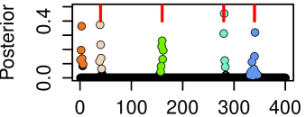
Figure 3: Example multiple change points. We simulate $T=400$ independent Gaussian random variables with four changes in variance ($K=4$, red segments depict true change points locations) and mean zero. We fit PRISCA with $L=8$ and $a_{0}=.001$ using Algorithm 1. Figure depicts the vectors $\bm{\alpha}_{l}$ for $l=1$ to $8$. The colored dots depict the five $\mathcal{CS}(.9)$ constructed. The remaining three $\bm{\alpha}$ are too diffuse.

The posterior distribution of PRISCA is not available in a tractable form, and we will approximate it with the algorithm discussed next. Now, we illustrate the discussion above with an example. We simulate a sequence of Gaussian random variables with four changes in variance, mean zero, and $\sigma^{2}=2$ (details in Figure 3 caption), and approximate the posterior distribution setting $L=8$. Figure 3 depicts the eight vectors $\bm{\alpha}_{1:8}$ (one of top each other); the approximate posterior distributions $[p(\bm{\gamma}_{l}|\textbf{y})]_{1:8}$. We colored five separate $90\%$ credible sets that have been constructed for the vector $\bm{\alpha}_{l}$ that “concentrate” around a time instance (more details in the next subsection). Note that while $K=4$, PRISCA detected an extra time change at the beginning of the sequence. The reason is that our implementation assumes that the baseline variance $\sigma^{2}$ is equal to one. Since this is not the case in this example, the algorithm correctly inferred a change at the beginning of the sequence. Three vectors were redundant because there was no remaining effect to capture. We observe here that they “do not concentrate” around any instance, i.e., they are diffuse.

3.2 How to fit PRISCA

A Gibbs sampler for PRISCA is readily available because the prior distributions in (3.1) are conditionally conjugate. However, such a chain is poised to mix very slowly because the random vectors $\bm{\gamma}_{l}$ are highly dependent. The deployment of MCMC in Bayesian change point detection commonly suffers from this problem, and lacking a very good initialization (e.g., the output of another change point detection procedure), chains often fail to converge; see Cappello et al. (2021).

The conditionally conjugate structure that makes writing a Gibbs sampler possible suggests a link to techniques used to solve additive models, as first noted by Hastie and Tibshirani (2000) and more recently by Wang et al. (2020). By construction, if one somehow removes the randomness of $(\gamma_{l^{\prime}},\tau_{l^{\prime}})_{l^{\prime}\neq l}$, the posterior update of $(\gamma_{l},\tau_{l})$ is the same as in the single change point problem. In a Gibbs sampler, the update relies on conditioning on the latest parameters’ update; in an additive model, the update relies on being able to compute residuals using previous iterations. In our setting, if we had access to $(\overline{\tau}^{2}_{l^{\prime}})_{l^{\prime}\neq l}$, the squared residuals of model (3.1) would be $\overline{r}_{l}^{2}=Y^{2}\circ\prod_{l^{\prime}\neq l}\overline{\tau}_{l}^{2}$, and one would obtain the posterior distribution $\mathrm{pr}(\gamma_{l},\tau_{l}|\overline{r}_{l})$ simply through (3)-(4). Clearly, $\mathrm{pr}(\gamma_{l},\tau_{l}|\overline{r}_{l})$ is not $\mathrm{pr}(\gamma_{l},\tau_{l}|Y)$ but it is at least a reasonable approximation, and it saves us a lot of computations because it bypasses the intractability of $\mathrm{pr}(\gamma_{l},\tau_{l}|Y)$. We will see that it is also a good approximation. Quite essentially, $\mathrm{pr}(\gamma_{l},\tau_{l}|\overline{r}_{l})$ allows for approximating $\overline{\tau}^{2}_{l}$ through (7), which in turns can be used to compute residuals for other effects. This reasoning suggests an iterative algorithm to approximate the posterior of PRISCA.

Algorithm 1 describes the recursion. It requires an initialization for $(\overline{\bm{\tau}}^{2}_{l})_{1:L}$ because one does not have access to them. For simplicity, we set them equal to vectors of ones, i.e., null effects. Then iteratively, the posterior distribution of each effect $(\bm{\tau}_{l},\bm{\gamma}_{l})$ is computed using the single change point updates (3)-(4), with the difference that one uses residuals $\overline{\textbf{r}}_{l}$ in lieu of y. Since we are not considering an additive model, we will not obtain the residuals by subtracting the expectation of each effect (except the one we are updating); instead, we scale y using $(p(\bm{\gamma}_{i},\bm{\tau}_{i}|\overline{\textbf{r}}_{i}))_{i\neq l}$. The rest proceeds in the same fashion as additive models, employing backfitting (Friedman and Stuetzle, 1981; Breiman and Friedman, 1985) to reduce the dependency on the order we fit each effect. The stopping rule is discussed in the next subsection. As highlighted by Wang et al. (2020), a difference with additive model is that every update does not give a new parameter estimate, rather a new distribution $p(\bm{\gamma}_{l},\bm{\tau}_{l}|\overline{\textbf{r}}_{l})$, fully defined by the vectors of probabilities $\bm{\alpha}_{l}$ and parameters $(a_{t,l},b_{t,l})_{t=1:T}$.

Algorithm 1 Fit of ProSCALE

Inputs: y, L, $a_{0}$, $\epsilon$

Output: $(\bm{\alpha}_{l})_{1:L}$, $[a_{t,l},b_{t,l}]_{l=1:L,t=1:T}$

1. Initialize setting all entries of $(\overline{\bm{\tau}}_{l}^{2})_{1:L}$ equal to one

2. Repeat until convergence

   For $l$ in $1$ to $L$

   • $\overline{\textbf{r}}_{l}^{2}=\textbf{y}^{2}\circ\prod_{l^{\prime}\neq l}\overline{\bm{\tau}}_{l^{\prime}}^{2}$

   • Update $\bm{\alpha}_{l}$, $[a_{t,l},b_{t,l}]_{t=1:T}$ via (3)-(4) using $\overline{\textbf{r}}_{l}^{2}$ in lieu of $\textbf{y}^{2}$

   • Update $\overline{\bm{\tau}}_{l}$ via (7)

   • Compute convergence criterion

   • Exit when convergence criterion variation is less than $\epsilon$

Algorithm 1 outputs $L$ vectors $\bm{\alpha}_{l}$ and the matrix $[a_{t,l},b_{t,l}]_{l=1:L,t=1:T}$. Each vector can be processed independently to give a point estimate and a credible set. When $L>K$, there are $L-K$ redundant vectors that should not capture any effect, and we expect the corresponding vector $\bm{\alpha}$ to be fairly flat. No matter what $\bm{\alpha}$ looks like, criteria (5)-(6) will return a point estimate and a credible set, even with $\bm{\alpha}$ is as in Figure 2 (B) bottom panel. Such behavior is not desirable. We employ a detection threshold to prevent that, classifying a change point as detected if its corresponding credible set is of cardinality less or equal to half of the sequence length. Thus,

$$\hat{K}=|\{\mathcal{CS}(\bm{\alpha}_{l},p):|\mathcal{CS}(\bm{\alpha}_{l},p)|\leq T/2\}|.$$ (9)

The threshold $T/2$ is somewhat arbitrary, but our results tend to be entirely insensitive for this threshold as $\bm{\alpha}$ is either very diffuse or very concentrated.

One could wonder whether an alternative to the $L-K$ redundant vectors being flats is two or more $\alpha_{l}$ concentrating around the same or a similar time instance. While in theory, this could happen, empirically, we see this happening only in the first algorithm’s iterations and then disappear as we iterate the algorithm until convergence via backfitting (see below). Nevertheless, in the implementation, we also include a postprocessing step that removes overlapping credible sets, as done by Wang et al. (2020). We study this issue in the supplementary material (Section S2).

To choose $L$, one could have prior information over $K$, as in the liver procurement example. In which case, the choice is simple as we can set it equal to that. Lacking prior knowledge, a heuristic is to run Algorithm 1 for multiple $L$s starting from one, and stop to increase $L$ when $\hat{K}$ stops rising. We call such a heuristic auto-PRISCA, because it is essentially parameter free since $L$ is not required and the algorithm is not sensitive to $a_{0}$ as long as it is small. A final possibility is to use the localization rate $\sqrt{T\log T}$ as the minimum spacing condition and set $L$ equal to a number proportional to $T/\sqrt{T\log T}$.

Finally, we notice that each iteration of Algorithm 1 requires a worst-case cost of $O(TL)$. This is not a problem in practice since the algorithm typically requires a small number of iterations to converge. Thus, for typical datasets Algorithm 1 has an effective overall computational complexity of $O(TL)$.

3.3 Convergence: Algorithm 1 as Variational Bayes

Algorithm 1 offers an efficient way to approximate PRISCA’s posterior distribution without sacrificing accuracy, as we will show in Section 4. The algorithm somewhat mimics the model’s rationale, with multiple single change point models fitted recursively. Although, it is clear that the output offers, at best, an approximation of the true posterior distribution. Given the remarkable empirical performance, a natural question is why Algorithm 1 works and whether there is an underlying model it approximates. In this subsection, we address this question and establish Algorithm 1’s convergence as a byproduct. Our result builds on Wang et al. (2020), who show that their recursive algorithm is a Variational Bayes (VB) approximation to the actual posterior distribution. Despite lacking an additive structure, we will show similar results in our context. Roughly, we are able to show that what holds for the Gaussian location parameter (Wang et al., 2020), is also true for the scale one using our construction.

Let $p$ denote the target posterior distribution. Given that $p$ is seldomly available in closed-form, a popular way to approximate $p$ is VB (Wainwright et al., 2008): let $\mathcal{Q}$ be an arbitrary family of distributions, one chooses $q\in\mathcal{Q}$ to approximate $p$ with minimal Kullback-Leibler divergence (Kullback and Leibler, 1951) between $q$ and $p$, i.e., $q=\operatorname*{arg\,min}_{q\in\mathcal{Q}}KL(q||p)$. If we do not restrict $\mathcal{Q}$ and can solve the resulting optimization problem, we can achieve $KL(q||p)=0$, which corresponds to $q\equiv p$. It means that, under no restrictions on $\mathcal{Q}$, we are simply formulating the problem of calculating the posterior as an optimization problem. VB becomes an approximation when we restrict the class $\mathcal{Q}$. Such restriction is chosen to make the optimization problem tractable; for example, Mean-Field VB (MFVB) assumes that the variational distribution $q$ factorizes over the variable of interests (Wainwright et al., 2008).

Even when imposing restrictions on $\mathcal{Q}$, one seldomly minimizes the KL divergence. The standard is to maximize the “evidence lower bound” (ELBO), given by the following equality

$$KL(q||p)=\int q(\theta)\log\frac{q(\theta)}{p(\theta|\textbf{y})}{\rm d}\theta=\log p(\textbf{y})-\int q(\theta)\log\frac{p(\textbf{y},\theta)}{q(\theta)}{\rm d}\theta=\log p(\textbf{y})-ELBO(q,\pi,\textbf{y}),$$

where $\pi$ denotes the prior distribution on the parameter $\theta$. We are making explicit the dependence of $ELBO(q,\pi,Y)$ on the prior distribution $\pi$, which is implicit in $p(y,\theta)$. The $\arg\max_{q\in\mathcal{Q}}ELBO(q,\pi,Y)$ is equivalent to the minimizer of $KL(q||p)$ because the marginal log-likelihood $\log p(Y)$ does not depend on $q$. The advantage of working with the ELBO is that the optimization can be solved analytically in several instances (Bishop, 2006).

Let $\mathcal{T}^{2}$ be a $T\times T$ diagonal matrix with entries $\bm{\tau}^{2}$, $\mathcal{T}_{l}^{2}$, the corresponding matrices with entries $\bm{\tau}^{2}_{l}$, and $|\cdot|$ the determinant. The posterior we want to approximate is $p(\bm{\tau}^{2}_{1:L},\bm{\gamma}_{1:L}|\textbf{y},\sigma^{2})$, and the model’s ELBO is

$$ELBO(q,\pi,\textbf{y}) :=\mathbb{E}_{q}[\log p(\textbf{y}|\bm{\tau}^{2}_{1:L},\bm{\gamma}_{1:L},\sigma^{2})]+\mathbb{E}_{q}\bigg{[}\log\frac{\pi(\bm{\tau}^{2}_{1:L},\bm{\gamma}_{1:L})}{q(\bm{\tau}^{2}_{1:L},\bm{\gamma}_{1:L})}\bigg{]}$$ (10)

$$=-\mathbb{E}_{q}\bigg{[}\frac{\log|\mathcal{T}^{2}|}{2}\bigg{]}-\mathbb{E}_{q}\bigg{[}\frac{\textbf{y}^{T}\mathcal{T}^{2}\textbf{y}}{2\sigma^{2}}\bigg{]}+\mathbb{E}_{q}\bigg{[}\log\frac{\pi(\bm{\tau}^{2}_{1:L},\bm{\gamma}_{1:L})}{q(\bm{\tau}^{2}_{1:L},\bm{\gamma}_{1:L})}\bigg{]}+\text{const.},$$

where the expected values are computed with respect to $q(\bm{\tau}^{2}_{1:L},\bm{\gamma}_{1:L})$. If we assume that $q$ factorizes over each component through the following mean-field assumption

$$q(\bm{\tau}^{2}_{1:L},\bm{\gamma}_{1:L})=\prod_{l}q_{l}(\bm{\tau}^{2}_{l},\bm{\gamma}_{l}),$$ (11)

we can further simplify the above as a function of expected values computed with respect to the individual $q_{l}$

$$ELBO(q,\pi,\textbf{y})=-\sum_{l}\mathbb{E}_{q_{l}}\bigg{[}\frac{\log|\mathcal{T}_{l}^{2}|}{2}\bigg{]}-\sum_{t}\frac{y^{2}_{t}\prod_{l}\mathbb{E}_{q_{l}}[\tau^{2}_{t,l}]}{2\sigma^{2}}+\sum_{l}\mathbb{E}_{q_{l}}\bigg{[}\log\frac{g_{l}(\bm{\tau}^{2}_{l},\bm{\gamma}_{l})}{q_{l}(\bm{\tau}^{2}_{l},\bm{\gamma}_{l})}\bigg{]}+\text{const.},$$ (12)

where $\mathbb{E}_{q_{l}}[\tau^{2}_{t,l}]$ can be computed analytically via (7). The contribution to $ELBO(q,\pi,\textbf{y})$ relative to the $l$th effect is

$$ELBO_{l}(q_{l},\pi_{l},\textbf{y}):=-\mathbb{E}_{q_{l}}\bigg{[}\frac{\log|\mathcal{T}^{2}_{l}|}{2}\bigg{]}-\mathbb{E}_{q_{l}}\bigg{[}\frac{\textbf{y}^{T}\mathcal{T}_{l}^{2}\textbf{y}}{2\sigma^{2}}\bigg{]}+\mathbb{E}_{q_{l}}\bigg{[}\log\frac{g_{l}(\bm{\tau}^{2}_{l},\bm{\gamma}_{l})}{q_{l}(\bm{\tau}^{2}_{l},\bm{\gamma}_{l})}\bigg{]},$$ (13)

where the second term is $\sum_{t}y^{2}_{t}\mathbb{E}_{q_{l}}[\tau^{2}_{t,l}]/2\sigma^{2}$. We are now ready to state the key result of the subsection.

Proposition 1.

Let $\overline{\textbf{r}}_{l}^{2}=\textbf{y}^{2}\circ\prod_{l^{\prime}\neq l}\overline{\bm{\tau}}_{l^{\prime}}^{2}$ be the residuals and $\pi_{l}$ be the prior distributions on $\bm{\tau}^{2}_{l}$ and $\bm{\gamma}_{l}$ given in (3.1). Then we have that

$$\operatorname*{arg\,max}_{q_{l}}ELBO(q,\pi,\textbf{y})=\operatorname*{arg\,max}_{q_{l}}ELBO_{l}(q_{l},\pi_{l},\overline{\textbf{r}}_{l}).$$

Proof.

The dependence on $q_{l}$ of the first and third terms of $ELBO(q,\pi,\textbf{y})$ is the same as that of $ELBO_{l}(q_{l},\pi_{l},\overline{\textbf{r}}_{l})$. To see that the dependence on $q_{l}$ of the corresponding terms is also the same, we rewrite it as

$$\sum_{t}\frac{y^{2}_{t}\prod_{l}\mathbb{E}_{q_{l}}[\tau^{2}_{t,l}]}{2\sigma^{2}}=\sum_{t}\frac{\overline{r}_{t,l}^{2}\mathbb{E}_{q_{l}}[\tau^{2}_{t,l}]}{2\sigma^{2}}=\mathbb{E}_{q_{l}}\bigg{[}\frac{\overline{\textbf{r}}_{l}^{T}\mathcal{T}_{l}^{2}\overline{\textbf{r}}_{l}}{2\sigma^{2}}\bigg{]}.$$

The claim then follows. ∎

Corollary 1.

The solution to the maximization in Proposition 1 is the posterior distribution of the single change point model defined in (2)-(3)-(4), where parameters $\bm{\alpha}_{l},(a_{t,l},b_{t,l})_{t=1:T}$ are computed using $\overline{\textbf{r}}_{l}^{2}$.

Proposition 1 and Corollary 1 establish that Algorithm 1 is a VB approximation to the posterior distribution of PRISCA, where the approximation lies in the fact that we have factorized the $L$ effects using a mean-field approximation. Corollary 1 holds because we did not restrict $q_{l}$ to belong to a particular family. Hence, the maximizer of $ELBO_{l}$ is the distribution $q_{l}$ that makes the $KL$ divergence between $q_{l}$ and the posterior distribution of a single change point model equal zero.

Proposition 1 formalizes that each step of Algorithm 1 maximizes the component-wise ELBO. I.e., the procedure to fit PRISCA is a block-wise coordinate ascent. The second result of the subsection follows.

Proposition 2.

Assuming $0<a_{0},\sigma^{2}<\infty$, the sequence $(\bm{\alpha}_{l,i})_{1:L,i\geq 1}$, $[a_{t,l,i},b_{t,l}]_{l=1:L,t=1:T,i\geq 1}$ defined Algorithm 1 converges to a stationary point of $ELBO(q,\pi,\textbf{y})$.

The convergence to a stationary point follows standard results on block-wise coordinate ascent Bertsekas (1999); Ortega and Rheinboldt (2000). With the condition on the hyperparameters, we require the posterior distribution of each “single change point problem” we solve to be properly defined.

4 Simulations

Table 1: Simulation study. Averages across $300$ repetitions for different sample sizes (T): bias $K-\widehat{K}$ (the lower, the better), Hausdorff statistics $d(\widehat{\mathcal{C}},\mathcal{C}^{*})$ (the lower, the better), time (in seconds), average credible set length (length), and coverage of the sets conditional on detection (cond. cov.). PELT, BINSEG, and SEGNEI are point estimators, so it is not possible to give length and cond. cov. PRISCA has $L=\left\lfloor T/30\right\rfloor$. ora-PRISCA has $L=K$, auto-PRISCA $L$ is set automatically. $\mathcal{CS}$ of PRISCA-based methods and MCP are constructed at $p=0.9$.

T	Method	$K-\widehat{K}$	$d(\widehat{\mathcal{C}},\mathcal{C}^{*})$	Time	Length	Cond. Cov.
200	MCP	1.7	106.3	27.86	24.04	0.95
	auto-PRISCA	1.38	72.57	0.15	13.49	0.81
	BINSEG	2.08	117.72	0
	PELT	1.92	106.96	0
	PRISCA	1.49	79.48	0.01	13.33	0.82
	ora-PRISCA	1.45	77.74	0.01	14.6	0.83
	SEGNEI	1.63	103.94	0.21
500	MCP	2.64	182.12	219.8	57.37	0.99
	auto-PRISCA	2.03	110.89	0.61	18.99	0.82
	BINSEG	3.05	206.9	0.01
	PELT	2.73	175.9	0
	PRISCA	2.02	124.96	0.18	18.68	0.84
	ora-PRISCA	1.91	114.38	0.04	20.91	0.85
	SEGNEI	2.41	185.84	0.34
1000	MCP	4.21	360.61	1830.2	93.46	0.99
	auto-PRISCA	2.94	186.07	2.82	23	0.84
	BINSEG	3.91	342.04	0.01
	PELT	3.39	263.76	0.01
	PRISCA	2.55	200.83	1.69	23.91	0.86
	ora-PRISCA	2.55	181.32	0.17	26.21	0.86
	SEGNEI	3.22	301.04	1.1

To validate PRISCA, we simulate sequences of zero-mean Gaussian observations experiencing multiple changes in variance. The setup of the simulation study is inspired by Killick et al. (2012). We consider data sets with varying lengths ($T\in\{200,500,1000\}$), varying change point locations, and different variances within each segment. The number of changes is set to $K=\left\lfloor T^{1/2}/4\right\rfloor$. For each simulate data set, we sample new change point locations $\mathcal{C}=\{t_{1}^{*},\ldots,t_{K}^{*}\}$ from a uniform distribution on $\{2,\ldots,T-2\}$ with an additional constraint that the minimum spacing between change points is $\min\{T^{1/2},30\}$ ($T^{1/2}$ is justified by the localization rate, see Section 2.1). Variances within each segment ($\sigma^{2}_{1},\ldots,\sigma_{K+1}^{2}$) are $i.i.d.$ samples from a lognormal distribution with mean $0$ and standard deviation $\log(10)/2$. We generate $300$ data sets per $T$.

By design, the simulation study is challenging because variances in consecutive blocks ($\sigma^{2}_{i}$ and $\sigma^{2}_{i+1}$) have positive probability of being practically identical. What matters is the relative performance of PRISCA vis-a-vis state-of-the-art methods. We compare PRISCA’s point estimates to PELT (Killick et al., 2012), Binary Segmentation (BINSEG) (Scott and Knott, 1974), Segment Neighbourhoods (SEGNEI) (Auger and Lawrence, 1989) (the three methods are available in the R package changepoint; Killick and Eckley (2014)). We also include the Bayesian method MCP (Lindeløv, 2020), which efficiently implements the Gibbs sampler of Carlin et al. (1992). MCP is the only method that requires knowledge of the true number of change points. We can obtain both point estimates and credible sets from MCP posterior distributions using the same rules employed by PRISCA. We also include a comparison to the Bayesian method of Fearnhead (2006) in the supplementary material (Section S4). We do not add it in the manuscript because, to compare it to the other methods, we had to add a postprocessing step to obtain point estimates and credible sets. This affects the method’s performance and makes the comparison unfair.

To measure accuracy, we use $K-\widehat{K}$ to measure how well each estimator recovers the actual number of change points. We also consider a Hausdorff-like statistic $d(\widehat{\mathcal{C}},\mathcal{C}^{*})=\underset{\eta\in\mathcal{C}^{*}}{\max}\,\ \underset{x\in\widehat{\mathcal{C}}}{\min}|x-\eta|$ to assess how well each method estimates the true change points locations $t^{*}_{1},\ldots,t^{*}_{K}$. To evaluate PRISCA’s credible sets, we report the average coverage of each set conditional on detection. For this study, a changepoint is considered to be detected if PRISCA identifies its location within a distance of $\min\{T^{1/2},30\}/2$ of the true position. Such notion detection is used by Killick et al. (2012), and we borrowed it in this study. We also report the average sets’ length. These measures are not available for PELT, BINSEG, and SEGNEG because they provide only point estimates, but they are for MCP.

PRISCA’s parameters are set to $a_{0}=.001$ (i.e., uninformative Gamma prior; results are unaffected by $a_{0}$, see supplementary material Section S3), $L=\left\lfloor T/30\right\rfloor$, (i.e., the maximum number of change points is set equal to the minimum spacing condition times the sequence length), and $\epsilon=.001$ (ELBO convergence). We initialize the algorithm as if there were no change points ($(\overline{\bm{\tau}}_{l}^{2})_{1:L}$ equal to one), We also report results for auto-PRISCA ($L$ chosen automatically through the heuristic described in Section 3.2) and an “oracle” version of PRISCA (ora-PRISCA) where we assume knowledge of the correct number of changes, i.e., $L=K$. Table 1 summarizes the results.

As expected by the study construction, no method accurately estimates $K$ ($K-\widehat{K}$ positive on average), but PRISCA-based methods attain the lowest bias across sample sizes. Similarly, PRISCA-based methods report the lowest $d(\widehat{\mathcal{C}}|\mathcal{C}^{*})$. This suggests that our approach outperforms state-of-the-art methodologies in this particular simulation study. We do not claim that PRISCA is better than state-of-the-art estimators. Rather than it can achieve comparable performance as a point estimator while also providing a measure of uncertainty. Notably, it is orders of magnitude faster than competing Bayesian methodologies we tested.

Table 1 reports the summary measures on the credible sets (here, $p=0.9$). The average length is small, providing evidence that the sets are not dispersed and that the posterior distributions of $\gamma_{l}$ concentrate on few points. The maximum length sets across all datasets are always well below the $50\%$ threshold we use in our detection threshold. We can see that PRISCA’s sets do not attain the targeted $p$ level, but they are relatively close. This behavior is largely expected because VB estimates are known to underestimate uncertainty (Bishop, 2006). While the underestimation is exceptionally severe in some VB applications, it does not seem to be the case here, especially considering the challenging simulation study. In addition, we see that if we have prior knowledge on the number of change points (ora-PRISCA), the coverage improves.

Compared to other Bayesian methods, PRISCA-based methods have average run-times orders of magnitude smaller than MCP and Fearnhead (2006). In this example, PRISCA has lower bias and better recovery of change point locations. MCP’s sets are well above the targeted $p$ level, possibly obtained because the sets are much bigger; e.g., almost four times bigger for $T=1000$.

Finally, PRISCA and auto-PRISCA have practically identical performance across all metrics, with auto-PRISCA having just slightly average run times. Recall that auto-PRISCA is essentially parameter-free since the only relevant parameter ($L$) is set through a heuristic. Surprisingly, the knowledge of $K$ used in ora-PRISCA does not lead to dramatic improvement in performance, suggesting that our heuristics to choose $L$ are a viable replacement of a priori knowledge of $K$.

5 Extensions

PRISCA can be readily extended to a range of more realistic and challenging settings than the one considered. We discuss here a few and give more details in the supplementary material. The scope is mostly to illustrate how easily our framework can be generalized. We acknowledge the limitations of the algorithms discussed below, and that much research is required to understand their theoretical and empirical properties. This goes beyond the scope of the paper and we leave it to future work.

Smoothly changing mean. There are plenty of phenomena described by a stochastic process undergoing multiple variance change points in the presence of a smoothly varying mean trend (Gao et al., 2019). For example, the data considered in this paper exhibits such a pattern (liver temperatures, Figure 4; wave heights, Figure 5). A possible model is $Y_{t}\sim N(f_{t},\sigma_{t}^{2})$, $t$ in $1$ to $T$, with $f_{t}$ a smooth function (e.g., assume it belongs to a reproducing kernel Hilbert space) and $\sigma_{t}^{2}$ is piecewise constant with $K$ breakpoints and sparse, in the sense that $K<<T$. Gao et al. (2019) tackle the setting $K=1$ with an algorithm that iterates a penalized weighted least square to estimate $f_{t}$ and the detection of a single change point with a generalized likelihood ratio. Each step is fed using the residuals computed from the previous one.

Algorithm 1 has a similar recursive structure. Hence, we can add an extra step with a penalized weighted least square (e.g., Tibshirani (2014) trend filtering) designed to estimate $f_{t}$. An obvious choice for the weights required by weighted least square is the vector $\prod_{l=1}^{L}\overline{\bm{\tau}}_{l}$, which provides an estimate of the precision at all times. The resulting estimate $\hat{f}_{t}$ can be then used to compute residuals needed by PRISCA Algorithm 1. PRISCA plus the extra step (we will call it TF-PRISCA) outputs estimates of $f_{t}$, the number and locations of multiple change points, and credible sets. To our knowledge, there is no available method with these features. We study TF-PRISCA’s empirical accuracy (estimations of $K$ and $\mathcal{C}$) in the supplementary material (Section S5).

Autoregression. Time-varying variance model is a field with a long history in econometrics (Tyssedal and Tjøstheim, 1982; Tjøstheim and Paulsen, 1985; Potscher, 1989). Change point detection in the presence of dependent noise has also received considerable attention recently (Dette et al., 2020). Assume $Y_{t}=\sum_{i=t-1}^{t-r}\phi_{i}Y_{i}+\epsilon_{t}$, and $\epsilon_{t}\sim N(0,\sigma_{t}^{2})$, $t$ in $1$ to $T$, with $\sigma_{t}^{2}$ piecewise constant with $K$ breakpoints and sparse. For simplicity, assume that the order $r$ is known. The case of known AR coefficients $(\phi_{i})_{1:r}$ is uninteresting: one can compute the noise sequence $(\epsilon_{t})_{1:T}$ and fit PRISCA directly to it.

In the case of unknown AR coefficients, PRISCA’s extension is similar to the smoothly varying mean case. A simple solution is to add an extra iteration in Algorithm 1, which consists of a weighted least squares estimation of $(\phi_{i})_{1:r}$. Any method to estimate the coefficients could be employed. Estimates are then used to compute the residuals, which are then fed into the usual PRISCA pipeline. Supplementary material Section S6 illustrates PRISCA’s empirical performance.

Multiple observations per time point - Periodic data. Throughout the paper, we employed the standard assumption that a single sample is available per time point. However, there are situations where practitioners require a model that can accommodate multiple observations per time point. For example, this can happen if the reported data are binned into time intervals.

An interesting case of repeated observations is when measurements are taken cyclically (e.g., at every hour of the day, every day), and the observations process exhibit a periodic structure (e.g., there is a shift in the morning and one at night). There are different ways to deal with this setting (Lund et al., 2007; Ushakova et al., 2022). A possible solution is to consider each cycle as a complete realization of the process, resulting in multiple observations per time point. Here, the cycle length equals $T$, and $n_{t}$ is the number of samples at time $t$. Bayesian change point methods naturally handle multiple observations collected at a given instance (Liu et al., 2017; Cappello et al., 2021), and PRISCA is no exception. Supplementary material Section S7 provides an application of PRISCA in the case of periodic data.

6 Real data

6.1 Liver viability assessment

Figure 4: Liver procurement data. Top row: liver temperature profile at three random locations (temperature every $10$ min. for $24$hrs, first $2.5$hrs not included, $T=130$). Bottom row: posterior distribution of the change locations. Dots depicts the probability of a change point at that location. Crosses denote the points included in a $p=90\%$ credible set. Dashed lines correspond to point estimates of Gao et al. (2019)’ method.

It has been observed that donor risk is increasing, with a majority of organs classified as marginal. Viability assessment in organ transplantation is a challenging task of utmost importance (Panconesi et al., 2021). Current techniques are either invasive, e.g., a biopsy of the organ, or highly subjective, e.g., they rely on the physician’s judgment of the candidate organs. The former strategy runs the risk of ruining the organ, and the latter is too subjective, given the high number of parameters that must be monitored to assess viability. Much research focuses on replacing these two approaches. Machine perfusion technology have emerged as an alternative in solid organ transplantation and it is an area currently subject of intense research efforts (Friend, 2020).

Here, we analyze experimental data studying a novel dynamic organ preservation strategy, which consists in monitoring the whole organ surface temperature of a liver perfused with a physiologic perfusion fluid (modified Krebs’ solution) (Gao et al., 2019). The experiment records the surface temperatures of a lobe of a porcine liver at $36795$ spots every 10 minutes for $24$ hours. Each temperature profile consists of $T=130$ points because the first $2.5$ hours of data were discarded (it takes about two hours for the perfusion fluid to infuse and stabilize the liver completely). We have data for $100$ random locations. Figure 4 top panels depict temperature profiles at three random locations of the liver. A visual inspection suggests a time-varying mean, domain knowledge indicates one change in variance. Gao et al. (2019) method was developed with this specific task in mind.

To account for the trend, we employ TF-PRISCA (the extension of PRISCA including the trend filter to account for a change in means). We could similarly account for the trend simply by using the first-order difference of the temperatures. Results do not change. The choice is motivated by the fact that we compare our results with Gao et al. (2019)’ method. PRISCA’s parameters were set to $a_{0}=.001$, $\epsilon=10^{-5}$, and $L=2$ (one effect for the unknown baseline variance and a second one for the single change point). For the mean, we used the glmgen implementation of the trend filter (Tibshirani, 2014), with $k=2$, we employed a weighted least square solution, and $\lambda$ chosen via BIC. Figure 4 bottom panels depict the posterior distribution of $\bm{\gamma}$ at three locations obtained with TF-PRISCA along with the estimates of Gao et al. (2019) methodology. Crosses depict $p=0.9$ credible sets, dashed lines the point estimates given by Gao et al. (2019). Change points from $t=1$ to $t=5$ were excluded from the plots because they refer to the baseline $\sigma^{2}$ (see also Figure 3).

In two locations, Gao et al. (2019)’ points estimates are in TF-PRISCA credible sets. TF-PRISCA point estimates are off by one instance in these two cases. In the third location (last column), the point estimate of Gao et al. (2019) is not included in the credible set. A visual inspection supports a change in variance in both locations. We note that if we were to run PRISCA with an extra effect (i.e., $L=3$), we would also recover this second change point. However, the experimental design suggests the existence of a single change.

Gao et al. (2019) method applied to the $100$ available locations estimate the change points to happen around around $12$ hours $84\%$ of the time, with the remaining $16\%$ estimated at $t=76$. The rightmost panel depicts an example of one of the instances where the change is estimated around $14$ hours. In the latter locations, our method points out that there is evidence for a loss of viability at around $12$ hours as well, hinting that loss of viability was uniform in the different locations.

6.2 Oceanographic data

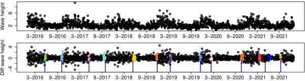
Figure 5: Oceanographic data. Top panel: daily ($T=2164)$ wave height (ft) recorded by buoy 46042 Monterey (NOOA data) in 2016-2021. Bottom panel: first-order difference of data in the top panel. Colors depict the time locations in the credible sets ($p=0.9$) constructed by PRISCA. Vertical blue segments depict PELT’s point estimates.

Practitioners who plan maintenance at offshore infrastructures, such as oil rigs and wind farms, study wave height volatility. A low wave height variation suggests stable sea conditions, which is necessary to minimize risks when organizing repairs and inspections offshore.

We consider wave height data collected hourly from January 2016 to December 2021 by Station 46042 Monterey, a buoy located twenty-seven miles off the coast of Monterey in the Pacific Ocean. The National Oceanic and Atmospheric Administration National Data Buoy center makes the data publicly available. Figure 5 depicts the sequence of observations subsampled such that we have one measure a day. We are not interested in modeling the seasonal trend – the mean wave height is high in winters and low in summers. To study changes in volatility, we model first-order differences as done by Killick et al. (2012) (TF-PRISCA could be alternatively used to account for the seasonal trend). Here, we use the first-order differences to compare our results with PELT.

Figure 5 depicts the change points locations obtained by PRISCA ($a_{0}=.001$, $L=30$, $\epsilon=10^{-5})$, its credible sets ($p=0.9$) along with PELT (point estimates, blue line). Rather than reporting the point estimates of PRISCA, we depict the credible sets coloring the time points. The segmentation of the two methods is practically identical, with two change points per year, one in autumn and one in spring. The methods differ in 2021, when PRISCA identifies an additional change point, with an extra segmentation in spring, while PELT estimates a single change point right in the middle of this segment. A visual inspection of the data suggests the possibility of an additional change point. The average length of the credible sets is $10.7$ days.

References

- (1)
- Anastasiou et al. (2022) Anastasiou, A., Cribben, I. and Fryzlewicz, P. (2022), ‘Cross-covariance isolate detect: a new change-point method for estimating dynamic functional connectivity’, Medical Image Analysis 75, 102252.
- Auger and Lawrence (1989) Auger, I. E. and Lawrence, C. E. (1989), ‘Algorithms for the optimal identification of segment neighborhoods’, Bulletin of Mathematical Biology 51(1), 39–54.
- Baranowski et al. (2019) Baranowski, R., Chen, Y. and Fryzlewicz, P. (2019), ‘Narrowest-over-threshold detection of multiple change points and change-point-like features’, Journal of the Royal Statistical Society: Series B (Statistical Methodology) 81(3), 649–672.
- Barnard (1959) Barnard, G. A. (1959), ‘Control charts and stochastic processes’, Journal of the Royal Statistical Society: Series B (Methodological) 21(2), 239–257.
- Barry and Hartigan (1992) Barry, D. and Hartigan, J. A. (1992), ‘Product partition models for change point problems’, The Annals of Statistics 20(1), 260–279.
- Barry and Hartigan (1993) Barry, D. and Hartigan, J. A. (1993), ‘A Bayesian analysis for change point problems’, Journal of the American Statistical Association 88(421), 309–319.
- Bertsekas (1999) Bertsekas, D. P. (1999), Nonlinear Programming, Athena Scientific, Belmont, MA.
- Bishop (2006) Bishop, C. M. (2006), Pattern recognition and machine learning, Vol. 4, Springer.
- Breiman and Friedman (1985) Breiman, L. and Friedman, J. H. (1985), ‘Estimating optimal transformations for multiple regression and correlation’, Journal of the American statistical Association 80(391), 580–598.
- Cappello et al. (2021) Cappello, L., Padilla, O. H. M. and Palacios, J. A. (2021), ‘Scalable Bayesian change point detection with spike and slab priors’, arXiv preprint arXiv:2106.10383 .
- Carlin et al. (1992) Carlin, B. P., Gelfand, A. E. and Smith, A. F. (1992), ‘Hierarchical bayesian analysis of changepoint problems’, Journal of the royal statistical society: series C (applied statistics) 41(2), 389–405.
- Chen and Gupta (1997) Chen, J. and Gupta, A. K. (1997), ‘Testing and locating variance changepoints with application to stock prices’, Journal of the American Statistical association 92(438), 739–747.
- Chen and Walker (2019) Chen, S. and Walker, S. G. (2019), ‘Fast Bayesian variable selection for high dimensional linear models: Marginal solo spike and slab priors’, Electronic Journal of Statistics 13(1), 284–309.
- Chernoff and Zacks (1964) Chernoff, H. and Zacks, S. (1964), ‘Estimating the current mean of a normal distribution which is subjected to changes in time’, The Annals of Mathematical Statistics 35(3), 999–1018.
- Dette et al. (2020) Dette, H., Eckle, T. and Vetter, M. (2020), ‘Multiscale change point detection for dependent data’, Scandinavian Journal of Statistics 47(4), 1243–1274.
- Fang and Siegmund (2020) Fang, X. and Siegmund, D. (2020), ‘Detection and estimation of local signals’, arXiv preprint arXiv:2004.08159 .
- Fearnhead (2006) Fearnhead, P. (2006), ‘Exact and efficient Bayesian inference for multiple changepoint problems’, Statistics and computing 16(2), 203–213.
- Frick et al. (2014) Frick, K., Munk, A. and Sieling, H. (2014), ‘Multiscale change point inference’, Journal of the Royal Statistical Society: Series B: Statistical Methodology 76(3), 495–580.
- Friedman and Stuetzle (1981) Friedman, J. H. and Stuetzle, W. (1981), ‘Projection pursuit regression’, Journal of the American statistical Association 76(376), 817–823.
- Friend (2020) Friend, P. J. (2020), ‘Strategies in organ preservation—a new golden age’, Transplantation 104(9), 1753–1755.
- Fryzlewicz (2014) Fryzlewicz, P. (2014), ‘Wild binary segmentation for multiple change-point detection’, The Annals of Statistics 42(6), 2243–2281.
- Fryzlewicz (2020) Fryzlewicz, P. (2020), ‘Narrowest significance pursuit: inference for multiple change-points in linear models’, arXiv preprint arXiv:2009.05431 .
- Gao and Owen (2017) Gao, K. and Owen, A. (2017), ‘Efficient moment calculations for variance components in large unbalanced crossed random effects models’, Electronic Journal of Statistics 11(1), 1235–1296.
- Gao et al. (2019) Gao, Z., Shang, Z., Du, P. and Robertson, J. L. (2019), ‘Variance change point detection under a smoothly-changing mean trend with application to liver procurement’, Journal of the American Statistical Association 114(526), 773–781.
- Hastie and Tibshirani (2000) Hastie, T. and Tibshirani, R. (2000), ‘Bayesian backfitting (with comments and a rejoinder by the authors’, Statistical Science 15(3), 196–223.
- Inclan and Tiao (1994) Inclan, C. and Tiao, G. C. (1994), ‘Use of cumulative sums of squares for retrospective detection of changes of variance’, Journal of the American Statistical Association 89(427), 913–923.
- Jewell et al. (2019) Jewell, S., Fearnhead, P. and Witten, D. (2019), ‘Testing for a change in mean after changepoint detection’, arXiv preprint arXiv:1910.04291 .
- Johndrow et al. (2020) Johndrow, J., Orenstein, P. and Bhattacharya, A. (2020), ‘Scalable approximate MCMC algorithms for the horseshoe prior’, Journal of Machine Learning Research 21(73).
- Killick and Eckley (2014) Killick, R. and Eckley, I. (2014), ‘changepoint: An r package for changepoint analysis’, Journal of statistical software 58(3), 1–19.
- Killick et al. (2012) Killick, R., Fearnhead, P. and Eckley, I. A. (2012), ‘Optimal detection of changepoints with a linear computational cost’, Journal of the American Statistical Association 107(500), 1590–1598.
- Kullback and Leibler (1951) Kullback, S. and Leibler, R. A. (1951), ‘On information and sufficiency’, The Annals of Mathematical Statistics 22(1), 79–86.
- Lai and Xing (2011) Lai, T. L. and Xing, H. (2011), ‘A simple Bayesian approach to multiple change-points’, Statistica Sinica pp. 539–569.
- Lindeløv (2020) Lindeløv, J. K. (2020), ‘mcp: An r package for regression with multiple change points’, OSF Preprints .
- Liu et al. (2017) Liu, C., Martin, R. and Shen, W. (2017), ‘Empirical priors and posterior concentration in a piecewise polynomial sequence model’, arXiv preprint arXiv:1712.03848 .
- Lund et al. (2007) Lund, R., Wang, X. L., Lu, Q. Q., Reeves, J., Gallagher, C. and Feng, Y. (2007), ‘Changepoint detection in periodic and autocorrelated time series’, Journal of Climate 20(20), 5178–5190.
- Ortega and Rheinboldt (2000) Ortega, J. M. and Rheinboldt, W. C. (2000), Iterative solution of nonlinear equations in several variables, SIAM.
- Padilla (2022) Padilla, O. H. M. (2022), ‘Variance estimation in graphs with the fused lasso’, arXiv preprint arXiv:2207.12638 .
- Page (1954) Page, E. S. (1954), ‘Continuous inspection schemes’, Biometrika 41(1/2), 100–115.
- Panconesi et al. (2021) Panconesi, R., Flores Carvalho, M., Mueller, M., Meierhofer, D., Dutkowski, P., Muiesan, P. and Schlegel, A. (2021), ‘Viability assessment in liver transplantation—what is the impact of dynamic organ preservation?’, Biomedicines 9(2), 161.
- Potscher (1989) Potscher, B. M. (1989), ‘Model selection under nonstationarity: Autoregressive models and stochastic linear regression models’, The Annals of Statistics pp. 1257–1274.
- Raftery and Akman (1986) Raftery, A. E. and Akman, V. E. (1986), ‘Bayesian analysis of a Poisson process with a change-point’, Biometrika pp. 85–89.
- Scott and Knott (1974) Scott, A. J. and Knott, M. (1974), ‘A cluster analysis method for grouping means in the analysis of variance’, Biometrics pp. 507–512.
- Siegmund (1986) Siegmund, D. (1986), ‘Boundary crossing probabilities and statistical applications’, The Annals of Statistics 14(2), 361–404.
- Smith (1975) Smith, A. F. (1975), ‘A Bayesian approach to inference about a change-point in a sequence of random variables’, Biometrika 62(2), 407–416.
- Tibshirani (2014) Tibshirani, R. J. (2014), ‘Adaptive piecewise polynomial estimation via trend filtering’, The Annals of Statistics 42(1), 285–323.
- Tjøstheim and Paulsen (1985) Tjøstheim, D. and Paulsen, J. (1985), ‘Least squares estimates and order determination procedures for autoregressive processes with a time dependent variance’, Journal of Time Series Analysis 6(2), 117–133.
- Tyssedal and Tjøstheim (1982) Tyssedal, J. S. and Tjøstheim, D. (1982), ‘Autoregressive processes with a time dependent variance’, Journal of Time Series Analysis 3(3), 209–217.
- Ushakova et al. (2022) Ushakova, A., Taylor, S. and Killick, R. (2022), ‘Multi-level changepoint inference for periodic data sequences’, Journal of Computational and Graphical Statistics .
- Wainwright et al. (2008) Wainwright, M. J., Jordan, M. I. et al. (2008), ‘Graphical models, exponential families, and variational inference’, Foundations and Trends in Machine Learning 1(1–2), 1–305.
- Wang et al. (2021a) Wang, D., Yu, Y. and Rinaldo, A. (2021a), ‘Optimal change point detection and localization in sparse dynamic networks’, The Annals of Statistics 49(1), 203–232.
- Wang et al. (2021b) Wang, D., Yu, Y. and Rinaldo, A. (2021b), ‘Optimal covariance change point localization in high dimensions’, Bernoulli 27(1), 554–575.
- Wang et al. (2020) Wang, G., Sarkar, A., Carbonetto, P. and Stephens, M. (2020), ‘A simple new approach to variable selection in regression, with application to genetic fine mapping’, Journal of the Royal Statistical Society: Series B (Statistical Methodology) 82(5), 1273–1300.
- Wang and Blei (2019) Wang, Y. and Blei, D. M. (2019), ‘Frequentist consistency of variational Bayes’, Journal of the American Statistical Association 114(527), 1147–1161.
- Worsley (1986) Worsley, K. J. (1986), ‘Confidence regions and tests for a change-point in a sequence of exponential family random variables’, Biometrika 73(1), 91–104.