Strain measurement by contour analysis

Abstract

The abstract is located on the next page for formatting reasons.

Abstract

Background: The determination of yield stress curves for ductile metals from uniaxial material tests is complicated by the presence of tri-axial stress states due to necking. A need exists for a straightforward solution to this problem.
Objective: This work presents a simple solution for this problem specific to axis-symmetric specimens. Equivalent uniaxial true strain and true stress, corrected for triaxiality effects, are calculated without resorting to inverse analysis methods.
Methods: A computer program is presented which takes shadow images from tensile tests, obtained in a backlight configuration. A single camera is sufficient as no stereoscopic effects need to be addressed. The specimen’s contours are digitally extracted, and strain is calculated from the contour change. At the same time, stress triaxiality is computed using a novel curvature fitting algorithm.
Results: The method is accurate as comparison with manufactured solutions obtained from Finite Element simulations show. Application to 303 stainless steel specimens at different levels of stress triaxiality show that equivalent uniaxial true stress – true strain relations are accurately recovered.
Conclusions: The here presented computer program solves a long-standing challenge in a straightforward manner. It is expected to be a useful tool for experimental strain analysis.

Keywords strain analysis; optical methods; tensile testing; stress triaxiality

1 Introduction

G’Sell et al. [1] were the first ones to perform strain analysis for cylindrical specimens using contour extraction from digital images. We revisit their idea and provide an estimation of the strain measurement accuracy by comparing against FEM simulation. The principle of the contour method is to measure the evolution of the diameter and compute the strain from the diameter change, assuming knowledge of how radial strain is related to longitudinal strain. This is, of course, trivial for ductile metals during plastic deformation, as this is typically an isochoric process.

The idea of G’Sell et al., to use a single camera with backlight illumination to obtain the specimen contours, seems not to have found many adopters, even though it is easy to use. Digital Image Correlation (DIC) techniques with their very general capability have replaced specialized techniques, and the contour analysis method is only applicable to cylindrical specimens in a straightforward manner. In our opinion, however, contour analysis provides a very good alternative to DIC in this special case, as it allows for evaluating the stress triaxiality. In this way, experimental force/displacement date can be directly converted to uniaxial true stress / true strain curves, suitable as input data for simulations.

A quite sophisticated approach to strain estimation by contour analysis was taken by Arthington et al. [2]. They used three projections of the contours, allowing them to compute also plastic Poisson’s ratio, thus eliminating the need for a-priori knowledge of this quantity. Although very promising, their approach lacks the simplicity of the original method and requires a – relatively – complex algorithm to post-process the image data. The aim of the work presented here is to provide theoretical background and an estimate of the accuracy to expect for the simple algorithm along with a publicly accessible open-source computer code for other researchers to use.

The remainder of this work is organized as follows. We begin by describing the method, and in particular, the salient feature of the computer algorithm used to evaluate the acquired images. Then, synthetic image data, obtained from FEM simulations, are used to analyze the accuracy of the method. Subsequently, the method is applied to tensile tests of a ductile stainless steel. Here, specimens with both notched and parallel gauge regions are considered, and the effects of stress triaxiality are quantified and removed from the data to yield uniaxial yield stress curves. Finally, we summarize our work by pointing out the strengths and weaknesses.

2 Description of the Method

2.1 Strain and stress measures

The purpose of this section is to define the stress and strain measures referred to in this work. We consider the true stress, which is the one-dimensional projection of the Cauchy stress, i.e., force per current cross section. The corresponding 1D strain measurement is the logarithmic strain. This pair of stress and strain measures is applicable for use with most large-deformation Finite Element codes. Such codes predominantly employ material models defined using true strain and true stress, assuming that the stress state is 1D.

The definition of true strain is

$$\varepsilon=\mathrm{ln}\frac{L}{L_{0}}$$ (1)

$L$ and $L_{0}$ are the current and initial length of a sample gauge region. We now restrict ourselves to axis-symmetric specimens only. In this case, the longitudinal strain may be calculated from the diameter change of the specimen. Referring to Fig. 1, and starting from the definition of Poissons’s ratio $\nu$, we have:

$$\nu = -\frac{\varepsilon}{\varepsilon_{\bot}}$$ (2)

$$\nu = -\frac{\varepsilon}{\mathrm{ln}\frac{\phi}{\phi_{0}}}$$ (3)

$$\varepsilon = \frac{1}{\nu}\;\mathrm{ln}\frac{\phi_{0}}{\phi}$$ (4)

Note that, in this context, $\nu$ does not refer only to the elastic Poisson’s ratio at infinitesimally small strains, but to the ratio of transverse to longitudinal strains for any deformation. $\nu$ must be known before Eq. 4 can be invoked. For many metals, however, plastic yielding is known to be an isochoric process with $\nu=0.5$, and we will assume in the following that $\nu$ is a known quantity. We will show below how the instantaneous diameter $\phi$ can be accurately identified from optical recordings, thus facilitating strain measurement.

With the instantaneous diameter known, the cross-section of axis-symmetric specimens is also known. Thus, the average stress in the specimen can be calculated with the instantaneous force,

$$\sigma_{avg}=\frac{F}{A}$$ (5)

Note, that $\sigma_{avg}$ is, in general, not equivalent to the 1D uniaxial true stress. This is only the case for a homogenous uniaxial deformation. If necking is present, additional radial and hoop stresses exist, which lead to an increase in the measured force compared to the case without necking. Thus, Eq. 5 will overestimate the uniaxial strength of a material when necking is present. This phenomenon, and a correction approach, was first described by P.W. Bridgman in 1952 [3]. He developed an approximate solution involving the current diameter $\phi$ and the radius of curvature $R$ of the neck, allowing to recover the uniaxial stress from the average stress:

$$\sigma\approxeq\sigma_{avg}\times\left[\left(1+\frac{4R}{\phi}\right)\mathrm{ln}\left(1+\frac{\phi}{4R}\right)\right]^{-1}$$ (6)

Numerous articles have investigated the validity of Bridgman’s assumptions and accuracy of his correction method, see e.g. [4, 5, 6, 7, 8]. A recent review [9] summarizes these works. The consensus seems to be that Bridgman’s correction produces errors less than 5% if both $\phi$ and $R$ are accurately known. Even better corrections are available, but these typically involve additional information about the material, e.g. the hardening exponent of the plastic yield curve, or additional numerical simulations. For the rest of this paper, we will use Bridgman’s original correction.

Bridgman also developed an expression for the stress triaxiality based on the ratio of $\phi$ and $R$. This quantity is important for failure models such as the Johnson-Cook model, where failure strain depends on the stress triaxiality. Bridgman’s original solution is

$$\eta\approxeq\frac{1}{3}+\mathrm{ln}\left(1+\frac{\phi}{4R}\right)$$ (7)

An improved correction method was found by Bai et al. [10] for the case of cylindrical specimens. This correction differs by an additional factor of $\sqrt{2}$, i.e.,

$$\eta\approxeq\frac{1}{3}+\sqrt{2}\mathrm{ln}\left(1+\frac{\phi}{4R}\right)$$ (8)

In this work we use the expression given by Bai et al..

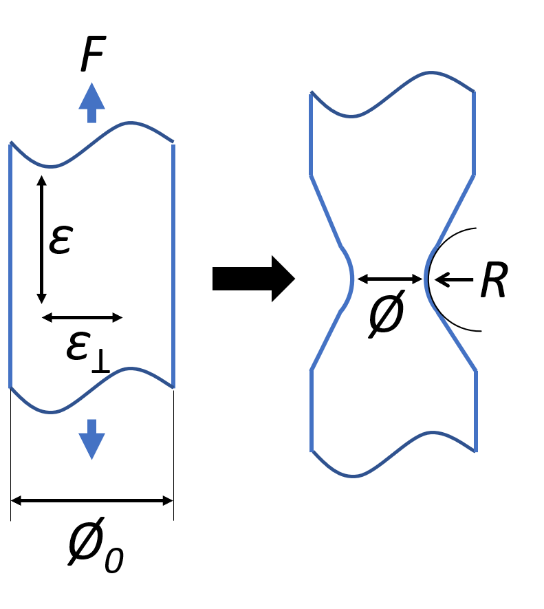
Figure 1: A cylindrical section is elongated due to the action of a force $F$. The longitudinal strain in the direction of the cylinder axis is denoted as $\varepsilon$, and the perpendicular strain is denoted as $\varepsilon_{\bot}$. The deformation leads to a diameter reduction from $\phi_{0}$ to $\phi$. For sufficiently large strains, necking with a local radius $R$ occurs.

2.2 Contour imaging

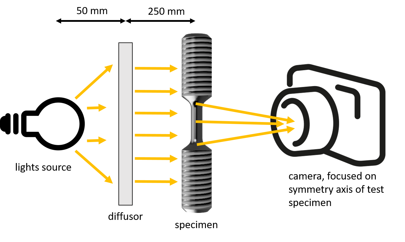
Figure 2: Setup of backlight contour imaging. A concentrated light source is diffused using a semi-transparent screen. The shadow image of a tensile test is recorded using a conventional camera. The focal plane of the camera is set to the symmetry axis of the cylindrical specimen.

To measure the specimen diameter and, eventually, the ensuing neck radius during a tensile test, a backlight technique is employed in this work. Fig. 2 shows the experimental setup. A light source is placed in front of a diffusing screen, e.g. semi-transparent plastic. A camera records shadow images of the specimen. It is important to set the center the focus plane onto the symmetry axis of the specimen. In this way, the radial contour does not move out of focus when the specimen diameter reduces as the tensile test progresses.

2.3 Contour analysis

Automatic extraction of the instantaneous minimum specimen diameter and the neck curvature around the image is accomplished by a computer program. Its source code is published online [11] and we discuss only its salient features here. The workflow is given in the following:

1. Load an ordered sequence of images and iterate over the set.

2. Binarize each image to black and white pixels only using Otsu’s adaptive thresholding method [12] which requires no predefined threshold.

3. Obtain the specimen’s contour from the contrast transition between white background and black specimen. For this, the Canny edge detector [13] is used with a Gaussian filter kernel of width $\phi_{0}/100$ px. The results of this operation are two contour lines.

4. Search for the location $x_{min}$ where the distance between the two contours is minimal. Store the current minimum diameter $\phi$.

5. For each contour line, determine the neck radius $R$. To this end, The neck region is identified in relation to the diameter: a subset of the contour, centered on $x_{min}$ and of length $\phi/2$ px is isolated. A circle is fit to this subset using Kanatani’s hyper-accurate method [14], which has been shown to compare favourably to other fitting methods [15].

6. With $\phi$ and $R$ known, compute the true strain and the triaxiality factor according to Eqns. 4 and 8. Also compute the current cross section $A=\pi\phi^{2}/4$, the average true stress ,and the corrected average stress according to Bridgman using Eqns. 5 and 6.

Note, that only two user-set parameters are required for this algorithm: The Canny edge kernel width and the extent of the necking region. Both are defined in relation to the current minimum specimen diameter and measured in pixel units. With the choices shown above, the algorithm produces typical strain errors smaller than 1% if the diameter $\phi$ is resolved with at least 200 px.

3 Validation with simulation data

To test the accuracy of the method, synthetic image data are prepared using the Finite Element code LS-Dyna. Two tensile specimen geometries are considered, one with a parallel gauge region, and one with a notch, see Fig. 3. The material model is chosen as elastoplastic with kinematic hardening, Young’s modulus of 70 GPa, Poisson’s ratio 0.3, initial yield stress 400 MPa and tangent modulus 100 MPa. $J_{2}$-plasticity with radial return is used. An axissymmetric discretization with a fine mesh size of  0.02 mm in the gauge region is used. Images of the simulation with white background and all-black finite elements are output at regular intervals, serving as synthetic experimental shadow images. These images are then analyzed using our algorithm and the results are reported in Fig. 4. For the purpose of comparison, the simulation data are evaluated as an average over the diameter of the gauge region, at the center of the neck. Fig. 4 A) shows that the total strain (elastic + plastic) at the center of the neck is well captured by the contour analysis for both specimen geometries. Fig. 4 B) compares the simulated stress triaxiality with the algorithm’s prediction using Eq. 8. The agreement is satisfactory, given the difficulty of estimating stress triaxiality otherwise, and the approximate nature of Eq. 8. A validation of the stress-strain relationship is presented in Fig. 4 C) and D). Here, the average stress is computed by our by contour analysis algorithm from the local true strain and the force, using Eq. 5. This stress is compared to the known stress/strain relation which was input to the simulation, denoted here as the material stress. It is evident that the stress computed in this way agrees well at small strains, but deviates for larger strains. The reason is the presence of stress triaxiality after the onset of necking. Correcting for this using Eq. 6, the corrected true stress is obtained, which agrees well with the known material stress: the maximum error is less than 2% for the specimen with parallel gauge region, and less than 5% for the notched sample.

The comparison with simulation data shows that the contour strain evaluation method is capable of measureing large strains with good accuracy, and estimating stress triaxiality with a sufficient accuracy such that equivalent uniaxial stress/strain curves can be obtained from experiment. The following section applies the method to real experiments.

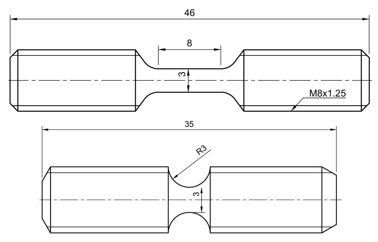
Figure 3: Sketch of the parallel and notched specimen geometries used in thios work. All dimensions are in mm.

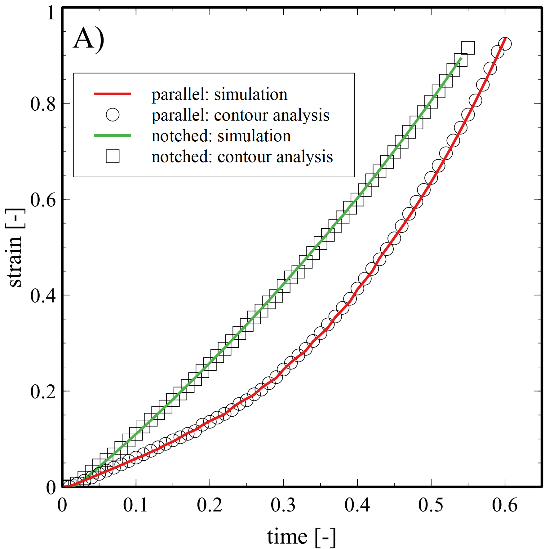
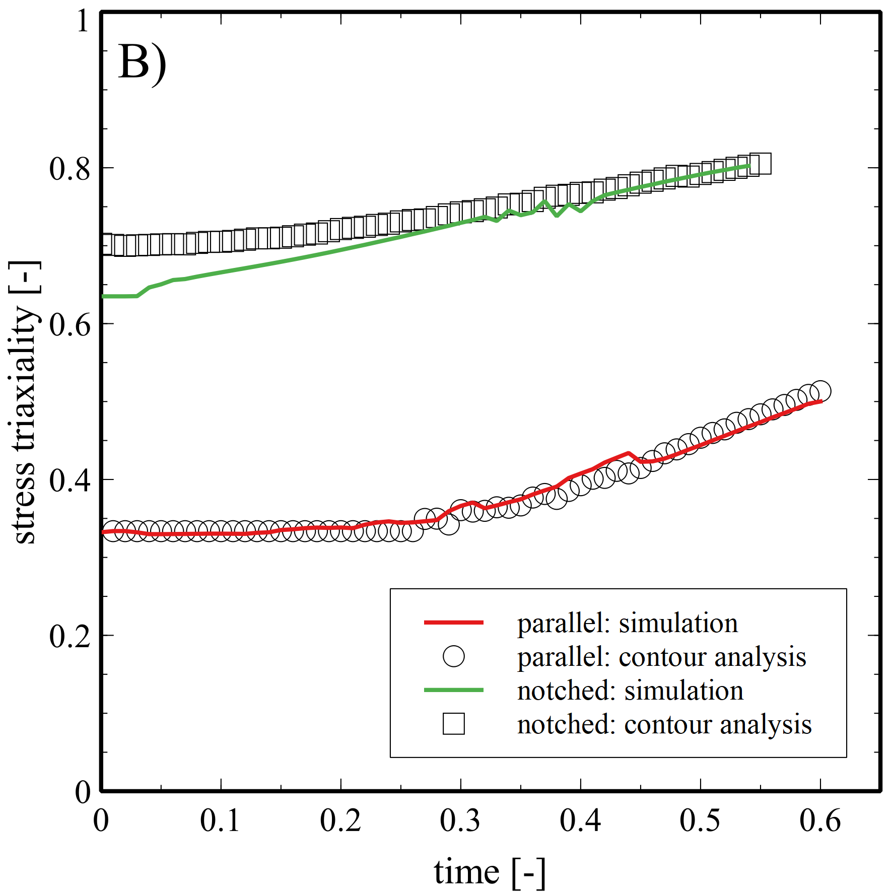
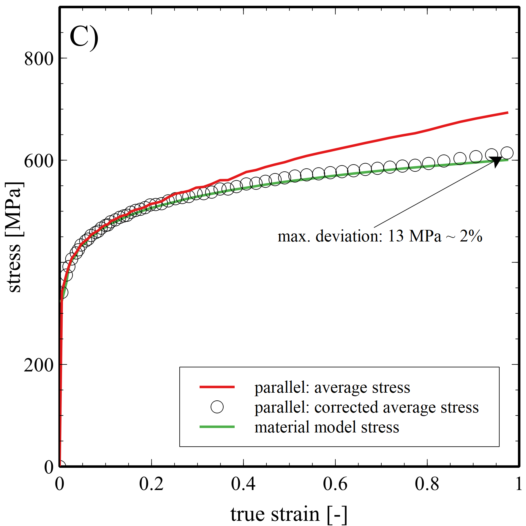
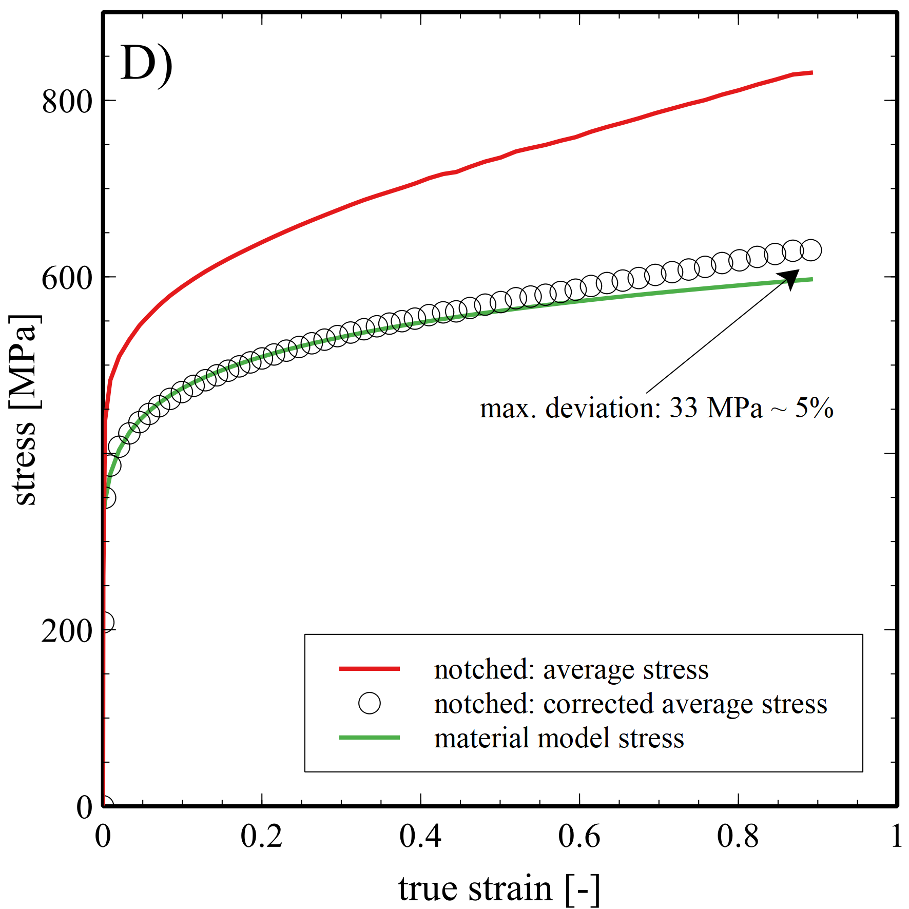
Figure 4: Comparison between exact simulation data and the results of our contour analysis algorithm. A$)$ compares total uniaxial strain for specimens with paralle and notched geometries with their simulation counterparts. B$)$ compares stress triaxiality between contour analysis and simulation. C$)$ and D$)$ show true average stress, c.f. Eq. 5, which overestimates the known material stress state if triaxiality effects are present. The same graphs also show the corrected true stress, obtained with Eq. 6, which agrees well with the known material stress. While C$)$ displays results for parallel gauge region specimen, while D$)$ shows results for a notched specimen.

4 Application to experiment

4.1 Materials

Specimens according to the dimensions shown in Fig. 3 were manufactured from stainless steel, AISI 303 (X8CrNiS18-9) using CNC turning from 10 mm bar stock. For this material, ultimate tensile strength is reported by the manufacturer as approximately 750 MPa.

4.2 Experiment setup

A universal testing machine (Zwick-Roell Z100) with a 100 kN load-cell (accuracy better than 0.1% of reading for force value > 200 N) is used in displacement control mode. The speed is set to 0.48 mm/min, corresponding to a nominal strain rate of $10^{-3}$ /s for the specimen with a parallel gauge region of 8 mm length. For imaging, a monochrome camera (Basler acA4112-20um) with 4096x3000 px resolution in combination with a 50 mm lens is used, such that the initial diameter of the specimen is resolved with $\phi_{0}~{}1000$ px. Background lighting is realised using a 50 W COB-LED with a light-emitting area of 24x40 mm² in combination with 3 mm thick white acrylic glass as a diffusor. Fig. 5 shows represenative images acquired during the experiment.

To compare the contour strain method with the established Digital Image Correlation (DIC) technique, a second camera with identical specifications is used. A speckle pattern is applied using an airbrush, resulting in typical speckle sizes of  8 px. The commercial DIC code GOM correlate is used with the default settings for this resolution of facet size of 51 px and point distance 20 px.

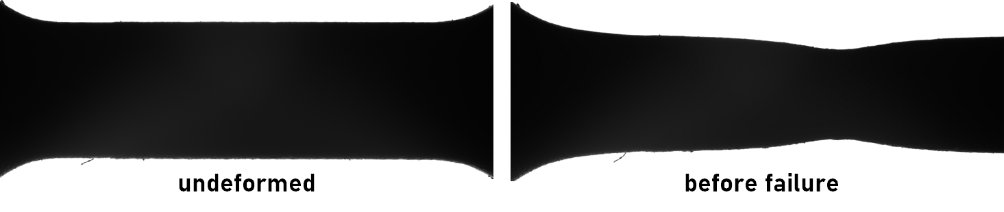
Figure 5: Unprocessed examples of acquired images for the straight specimen type considered in this work.

4.3 Results

Fig. 6 shows stress/strain data obtained using the methods described in this work. A total of 6 specimens with parallel gauge region 3 specimens with notched geometry were tested. Fig. 6 A shows nominal stress (engineering stress, force over initial cross-section area) over true strain, which is computed using contour analysis. The different specimens geometries are grouped tightly, indicating good specimen quality and repeatability of the analysis method. The curves for the notched specimens read approximately 160 MPa higher stress than the parallel gauge type specimens. This apparent stress enhancement is due to stress triaxiality. Average true stress over true strain, as defined in Eq. 5, is shown in Fig. 6 B. These curves are of strictly monotonous character. This is to be expected, as a negative slope (softening) would indicate material instability. However, the groups for the different specimens are still separated. Therefore, they do not yet present the underlying uniaxial material behaviour. This is of course obvious for the notched specimen geometry, which is affected from triaxiality effects already at small strains. The parallel gauge section specimens, however, undergo necking at a strain of approximately 35%. From this point onwards, they are also affected by stress triaxiality, and the average true stress is not a good measure for the underlying uniaxial stress/strain curve. Fig. 6 C shows that all data collapse onto a single stress/strain curve, if the corrected true stress according to Eq. 6 is considered, only the failure strains remain different. This demonstrates that this correction addresses the effects of stress triaxiality adequately. The resulting stress/strain data now represents the equivalent stress and equivalent strain for uniaxial loading, and may be used, e.g., as yield stress input curve for simulation purposes.

Comparison with the established strain measurement technique Digital Image Correlation is made in Fig. 6 D. The DIC evaluation window is limited to those facets which are located within the necking region only. At small strains, the agreement between both methods is good, but the accuracy of DIC is presumably quite better due sub-pixel interpolation. At large strains, close to specimen failure, strains reported by DIC are significantly lower than the strain values computed by contour analysis. This can be understood by the fact, that the regions used in DIC for strain evaluation cannot be made arbitrarily small. Thus, DIC values are smoothed in space. Additionally, the DIC speckle pattern deteriorates for large strains, DIC accuracy becomes questionable. This is of course strongly dependent on the magnitude of failure strain and the quality of the speckle pattern and optical recordings. Nevertheless, contour analysis is unaffected by these difficulties.

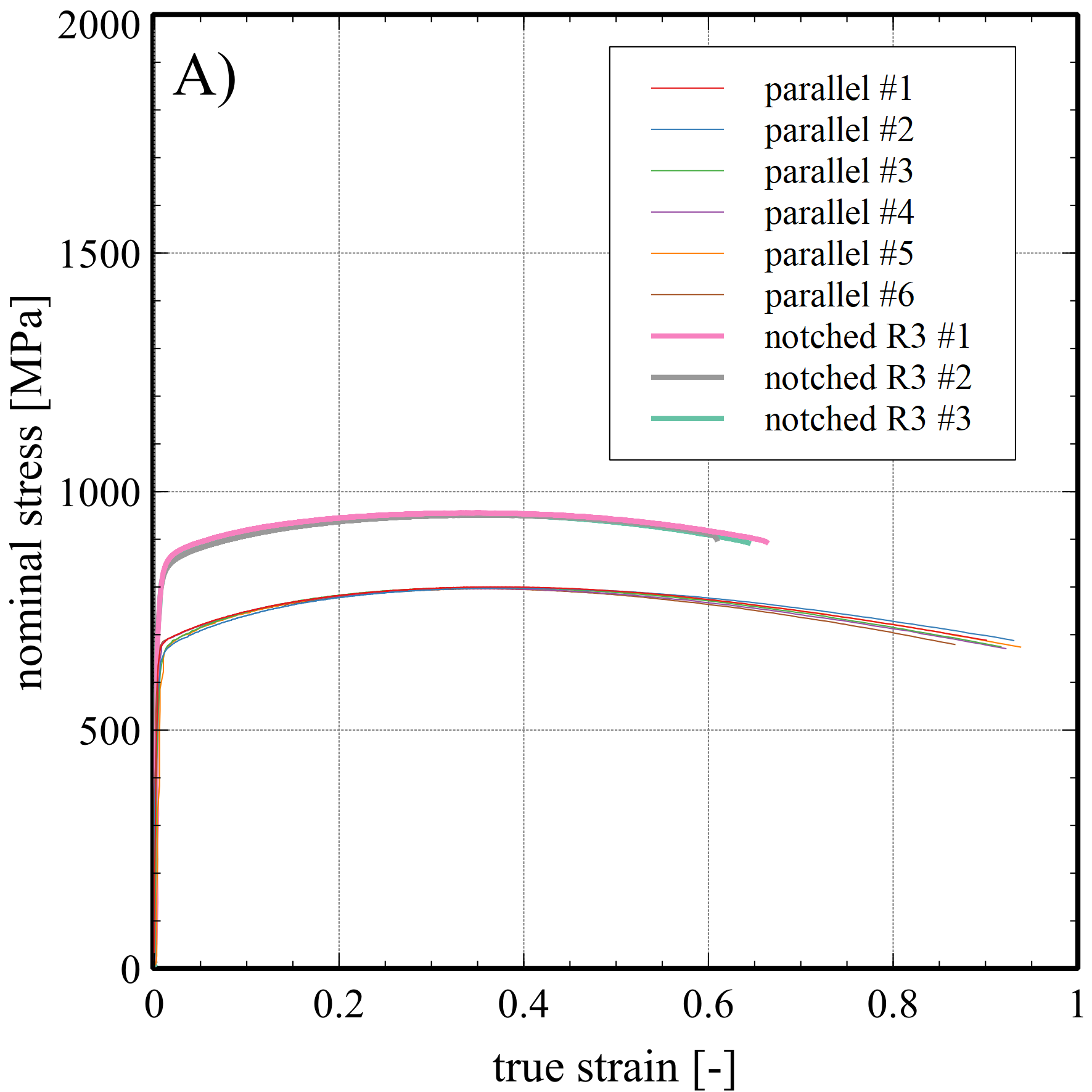
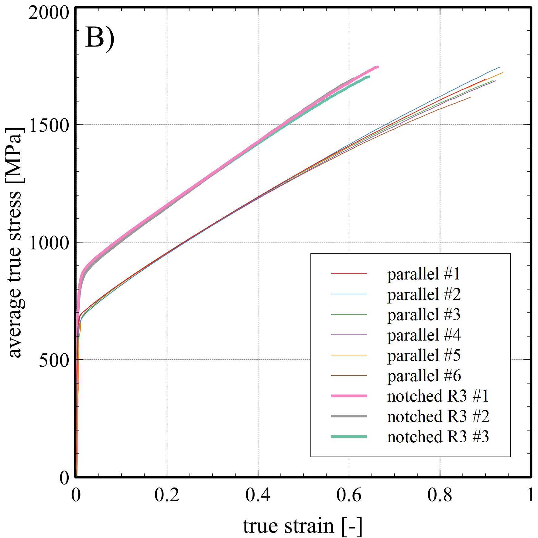
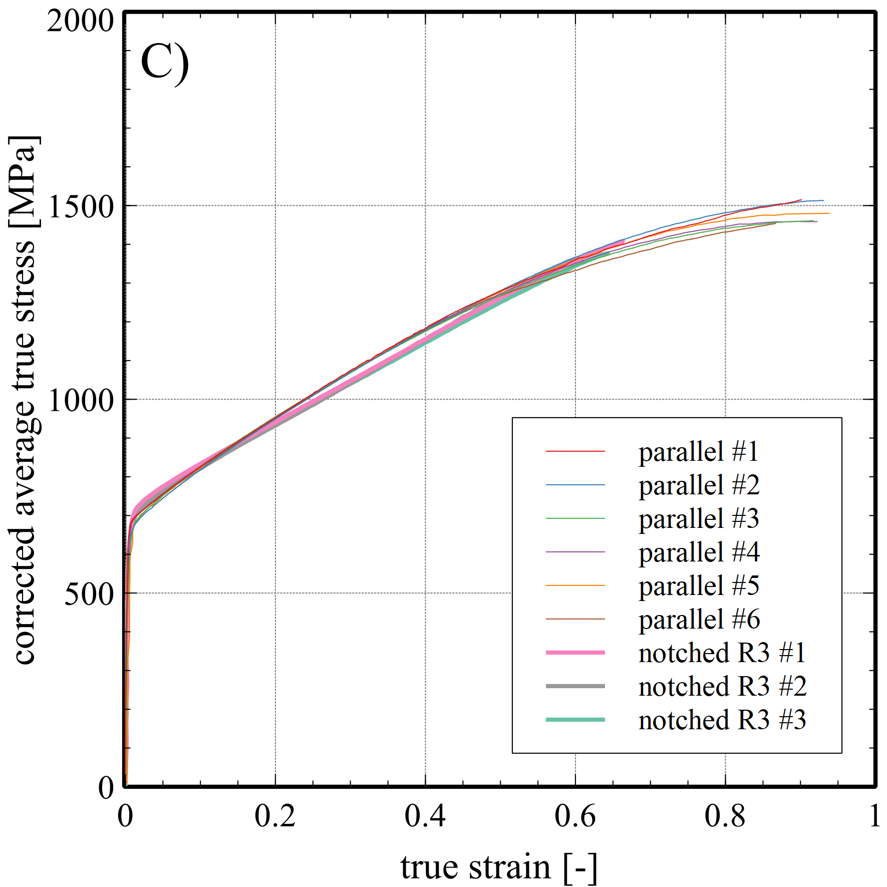
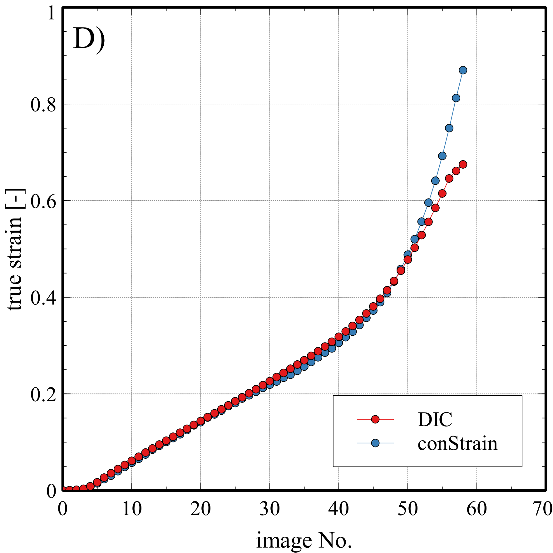
Figure 6: Experimentally determined stress-strain diagrams for stainless steel specimens with parallel and notched gauge regions. A$)$ shows nominal stress (c.f. equation nominal) over true strain (c.f. equation true strain). B$)$ shows true stress (c.f. equation nominal) over true strain (c.f. equation true strain). C$)$ shows true stress, corrected for triaxiality effects, (c.f. equation nominal), over true strain (c.f. equation true strain). The stress curves are clearly separated between notched and parallel specimen types in subfigures A$)$ and B$)$, but collapse onto each other once triaxiality effects are accounted for, as seen in subfigure C$)$. For one parallel gauge section specimen, comparison with DIC evaluation is shown in D$)$.

5 Discussion and conclusion

This work revisits the idea of G’Sell et al. [1], which is to compute true strain for axis-symmetric tensile specimens using optical contour analysis methods. In our interpretation of this, we use image processing techniques including the Canny-Edge filter [13] for contrast enhancement and a modern robust curvature fitting routine [14]. This allows us to not only measure true strain, but also estimate stress triaxiality. There are two major inherent limitations to this approach. It is only applicable to axis-symmetric specimens, and ratio of transversal strain to longitudinal strain must be known beforehand. Nevertheless, for ductile metals, this does not impose drastic limitations, as these typically obey isochoric during plastic deformation, and cylindrical specimen geometries are often used. Under these circumstances, the method provides a very convenient, and accurate measurement of the equivalent uniaxial true stress / true strain relationship as needed for constitutive modelling. This work shows, by comparison with manufactured solutions using FEM simulations, and application to real tensile tests, that this approach is practical and viable. The method requires only a single camera, as the contour does not move out of the focal plane. No 3D effects must be considered, as would otherwise be the case with the established DIC method [16]. Furthermore, no speckle pattern is required, as the method used a shadow image obtained with background illuminations. This means that contour strain analysis could be applied to extreme scenarios, such as high-temperature tensile tests, where a speckle pattern would thermally deteriorate. Our contour strain analysis technique provides a local strain measurement directly at the minimum diameter of a specimen. It is applicable to strong necking in ductile metals, where it also provides an estimate of the stress triaxiality. We believe that the technique is useful for experimental analysis and provide an opens source implementation of our program, termed conStrain [11].

Conflicts of Interest

The authors declare no competing interests.

References

- G’Sell et al. [1992] G’Sell C, Hiver JM, Dahoun A, Souahi A. Video-Controlled Tensile Testing of Polymers and Metals beyond the Necking Point. J Mater Sci 1992 Sep;27(18):5031–5039.
- Arthington et al. [2009] Arthington MR, Siviour CR, Petrinic N, Elliott BCF. Cross-Section Reconstruction during Uniaxial Loading. Meas Sci Technol 2009 Jun;20(7):075701.
- Bridgman [1952] Bridgman PW. Studies in Large Plastic Flow and Fracture with Special Emphasis on the Effects of Hydrostatic Pressure. New York: McGraw-Hill; 1952.
- Choung and Cho [2008] Choung JM, Cho SR. Study on True Stress Correction from Tensile Tests. J Mech Sci Technol 2008 Jun;22(6):1039–1051.
- Kweon et al. [2020] Kweon HD, Kim JW, Song O, Oh D. Determination of True Stress-Strain Curve of Type 304 and 316 Stainless Steels Using a Typical Tensile Test and Finite Element Analysis. Nuclear Engineering and Technology 2020 Jul;.
- Ling [1996] Ling Y. Uniaxial True Stress-Strain after Necking. AMP Journal of Technology 1996;5:37–48.
- Murata et al. [2018] Murata M, Yoshida Y, Nishiwaki T. Stress Correction Method for Flow Stress Identification by Tensile Test Using Notched Round Bar. Journal of Materials Processing Technology 2018 Jan;251:65–72.
- Wang et al. [2016] Wang Yd, Xu Sh, Ren Sb, Wang H. An Experimental-Numerical Combined Method to Determine the True Constitutive Relation of Tensile Specimens after Necking. Advances in Materials Science and Engineering 2016;2016:1–12.
- Tu et al. [2020] Tu S, Ren X, He J, Zhang Z. Stress–Strain Curves of Metallic Materials and Post-necking Strain Hardening Characterization: A Review. Fatigue Fract Eng Mater Struct 2020 Jan;43(1):3–19.
- Bai et al. [2009] Bai Y, Teng X, Wierzbicki T. On the Application of Stress Triaxiality Formula for Plane Strain Fracture Testing. Journal of Engineering Materials and Technology 2009 Apr;131(2):021002.
- Ganzenmüller [????] Ganzenmüller GC, conStrain – a Program to Perform Optical Contour Strain Analysis (to Be Made Available Online Together with Publishing of This Article). Freiburg, Germany;.
- Otsu [1979] Otsu N. A Threshold Selection Method from Gray-Level Histograms. IEEE Transactions on Systems, Man, and Cybernetics 1979 Jan;9(1):62–66.
- Canny [1986] Canny J. A Computational Approach to Edge Detection. IEEE Transactions on Pattern Analysis and Machine Intelligence 1986 Nov;PAMI-8(6):679–698.
- Kanatani [2006] Kanatani K. Ellipse Fitting with Hyperaccuracy. IEICE TRANSACTIONS on Information and Systems 2006 Oct;E89-D(10):2653–2660.
- Al-Sharadqah and Chernov [2009] Al-Sharadqah A, Chernov N. Error Analysis for Circle Fitting Algorithms. arXiv:09070421 [stat] 2009 Jul;.
- Weidner and Biermann [2021] Weidner A, Biermann H. Review on Strain Localization Phenomena Studied by High-Resolution Digital Image Correlation. Advanced Engineering Materials 2021;23(4):2001409.