Toward Unlimited Self-Learning MCMC with Parallel Adaptive Annealing
Abstract
Self-learning Monte Carlo (SLMC) methods are recently proposed to accelerate Markov chain Monte Carlo (MCMC) methods using a machine learning model. With latent generative models, SLMC methods realize efficient Monte Carlo updates with less autocorrelation. However, SLMC methods are difficult to directly apply to multimodal distributions for which training data are difficult to obtain. To solve the limitation, we propose “parallel adaptive annealing,” which makes SLMC methods directly apply to multimodal distributions with a gradually trained proposal while annealing target distribution. Parallel adaptive annealing is based on (i) sequential learning with annealing to inherit and update the model parameters, (ii) adaptive annealing to automatically detect under-learning, and (iii) parallel annealing to mitigate mode collapse of proposal models. We also propose VAE-SLMC method which utilizes a variational autoencoder (VAE) as a proposal of SLMC to make efficient parallel proposals independent of any previous state using recently clarified quantitative properties of VAE. Experiments validate that our method can proficiently obtain accurate samples from multiple multimodal toy distributions and practical multimodal posterior distributions, which is difficult to achieve with the existing SLMC methods.
1 INTRODUCTION
High-dimensional probability distributions for which the normalizing factor is not analyzable appear in a wide variety of fields. For example, they appear in condensed-matter physics (Binder et al., 1993; Baumgärtner et al., 2012), biochemistry (Manly, 2018), and Bayesian inference (Martin et al., 2011; Gelman et al., 1995; Foreman-Mackey et al., 2013). Markov chain Monte Carlo (MCMC) methods are powerful and versatile numerical methods for sampling from such probability distributions. Its efficiency strongly depends on the choice of the proposal.
Among recent advances in machine learning, a general method called the self-learning Monte Carlo (SLMC) method (Liu et al., 2017) was introduced to accelerate MCMC simulations by an automated proposal with a machine learning model and has been applied to various problems (Xu et al., 2017; Shen et al., 2018). In particular, a latent generative model realizes efficient global update through the obtained information-rich latent representation (Huang & Wang, 2017; Albergo et al., 2019; Monroe & Shen, 2022; Tanaka & Tomiya, 2017). Although powerful, the performance of SLMC simulation strongly depends on an automated proposal with machine learning models and the quality of training data to train the proposal. For example, it is challenging to directly use SLMC for multimodal distributions because obtaining accurate training data covering all modes is difficult.
In this paper, we propose a novel SLMC method to directly make the methods applicable to multimodal distributions and substantially expand the scope of application of the SLMC methods in various fields. Specifically, we introduce (i) sequential learning with annealing to inherit and update the model parameters for pre-train effect, like a simulated annealing (Kirkpatrick et al., 1983), (ii) adaptive annealing path for efficient and automatic detection of the under learning, (iii) parallel annealing method mitigates that the proposal does not generate all modes of the target distribution, i.e., “mode collapse” by ensemble learning effect. The resulting combination is called the “parallel adaptive annealing SLMC”. With only a simple annealing (i), under-learning and mode collapse of proposals typically lead to failure results, but parallel adaptive annealing can solve these problems and even speed up. This improvement significantly contributes to using SLMC methods for larger systems. Additionally, as an example of a proposal in this method, we propose a variational autoencoder (VAE) (Kingma & Welling, 2013), one of the latent generative models, as a proposal by applying the recently clarified quantitative property of VAEs (Nakagawa et al., 2021; Rolinek et al., 2019). Our contributions are summarized as follows:
-
•
Introduction of annealing for SLMC methods, which make SLMC methods directly applicable to multimodal distribution.
-
•
SLMC-specific parallel adaptive annealing method, which automatically detect and solve under-learning and mode collapse in annealing and even speed up the annealing.
-
•
Through numerical experiments, we demonstrate that parallel annealing method can solve the under-learning and mode collapse and also apply the method to various difficult problems.
2 BACKGROUND
2.1 Metropolis–Hastings Algorithm
We start this section by illustrating the Metropolis–Hastings method (Hastings, 1970). We define as a target distribution on a state space where the normalizing factor is not necessarily tractable. Then assume is tractable which can be expressed in closed form. To obtain samples from , we use an MCMC method to construct a Markov chain whose stationary distribution is . The objective of the MCMC method is to obtain a sequence of correlated samples from the target distribution , where the sequence can be used to compute an integral such as an expected value.
The Metropolis–Hastings algorithm is a generic method to construct the Markov chain (Hastings, 1970). The Metropolis–Hastings algorithm prepares a conditional distribution called a proposal distribution, which satisfies irreducibility, and the Markov chain proceeds via the following steps: starting from , where is the initial distribution, at each step , proposing , and with probability
accept as the next update or with probability , reject and retain the previous state . The proposal distribution is prepared for typically a local proposal, such as , where a scale parameter for the continuous probability distribution. Hereafter, such a method is referred to as a local update MCMC method. Note that the calculation of the acceptance probability only requires the ratio of probability distributions (i.e., calculation of the normalizing factor is not required). Note that the performance of the algorithm strongly depends on the choice of the proposal distribution .
2.2 Self-learning Monte Carlo
Motivated by the developments of machine learning, a general method, known as the self-learning Monte Carlo (SLMC) method, has been proposed. In this method, the information of samples generated by a local update MCMC method is extracted by a machine learning model and the MCMC simulation is accelerated with the model . Specifically, the SLMC method sets the proposal distribution as and the acceptance probability is expressed as
| (1) |
If we obtain a perfect machine learning model such that , the acceptance probability is . Moreover, if the proposal is accepted, the state will be uncorrelated with any previous state because the proposal probability is independent of the previous state .
Note that the machine learning model for the SLMC method is desired to have the following three properties:
-
1.
The model should have the expressive power to well approximate the target probability distribution .
-
2.
Both proposals and acceptance probabilities in Eq. (1) should be computed from the machine learning model at low cost.
-
3.
accurate training data should be available to train the machine learning model .
If the first property is unsatisfied, the proposed state is rarely accepted and the correlation between samples becomes large. If the second property is unsatisfied, then, even if a good machine learning model is obtained, the SLMC simulation will not be efficient because of the cost of proposing a new state and computing the acceptance probability in Eq. (1). If the third property is not satisfied, the SLMC method will generate biased samples in practical sense due to slow mixing, etc. because the model can hardly propose a state that is not included in the training data.
2.3 Theoretical results of VAE
A VAE (Kingma & Welling, 2013) is a latent generative model, and its purpose is to model the probability distribution behind the data. Let , be training data and be the empirical distribution of the training data. Specifically, the VAE is a probability model of the form , where is the latent variable with prior , which is a standard normal distribution widely used. The -VAE (Higgins et al., 2016) is trained by maximizing the following evidence lower bound (ELBO) of log-likelihood with variational posterior , where , is an estimating parameter, since direct maximization of the log-likelihood is difficult:
| (2) |
where and denote Kullback–Leibler divergence and ELBO, respectively. is introduced to control the trade-off between the first and second terms of Eq. (2). and are called a decoder and an encoder, respectively, and the first term in Eq. (2) is called a reconstruction loss.
Recently, extensive work has been done to clarify the theoretical properties of VAEs. In that theoretical analysis, we apply the following theorem (Rolinek et al., 2019; Nakagawa et al., 2021); see Supplementary Material B for detail of proof sketch.
Theorem 2.1.
Suppose that VAE satisfy the “polarized regime”, which the latent space can be partitioned as the disjoint union , such that; (a) , (b) . If the reconstruction loss is the sum of squared errors (SSE) and the prior is a standard normal distribution, then following holds:
| (3) |
under the optimally conditions of loss function Eq. 2. Here we denote and denotes an dimensional identity matrix.
Whether Eq. 3 holds, which is the key to the detailed valance, can be easily validated in the trained VAE model as shown in Supplementary Material C.1. Polarized regime is typically observed very early in the training, which is well-known to practitioners and is checked on multiple tasks and datasets, and the optimally conditions are easily reachable since Rolinek et al. (2019) shows that every local optimal solution is a global optimal solution. Here, and are regarded as subspaces of the data manifold which a VAE learned and out of the manifold, respectively. Accordingly, can be less than and must be larger than the dimension of the data manifold the VAE model can learn.
3 ANNEALING SELF-LEARNING MONTE CARLO WITH VAE
We introduce an annealing for SLMC methods to apply the methods to multi-modal distributions directly and clarify that simple annealing has two practical problems (under-learning and mode collapse). Then, we propose adaptive annealing to automatically detect under-learning of the proposal and parallel annealing to mitigate mode collapse of the proposal. In addition, we introduce a novel SLMC method with a VAE called “VAE-SLMC,” by applying the recently revealed theoretical results Eq. 3.
3.1 Annealing for SLMC methods
We start by introducing inverse temperature for a range of values to a target distribution and as
| (4) |
Note that becomes a target distribution. Typically, smaller allows easier exploration for multiple modes, even in the complex distribution. Our annealing for SLMC methods is based on increasing from a small value (i.e., high temperature) to 1, like simulated annealing.
The detailed flow of the annealing is abstracted in Fig. 1 and described following; First, we set up an annealing path , , where is set sufficiently small for the local update MCMC method to explore efficiently. Second, we acquire the training data from the by the local update MCMC method and train the model with the training data. Third, we acquire the training data again from the by the SLMC with the model and then train the model with the training data from . Note that the initial parameters of training the model are set as since and are expected to have a similar common structure, leading to a similar effect like “pre-training”. By repeating this process until , we finally obtain accurate samples from the target distribution .
Note that it is essential that the machine learning models not only satisfy the desired conditions explained in Sec. 2.2, but also learn multimodal distributions and easily propose all learned modes to create accurate training data covering modes of target distributions in the annealing. Additionally, simple annealing (e.g., simply setting an arithmetic progression annealing path and log-linear annealing path) often requires extra computation time and frequently lead to the following two problems, preventing SLMC methods from application to larger systems;
-
1.
under-learning: The acceptance rate decreases rapidly due to under-learning of the model while annealing.
-
2.
mode collapse: Although the acceptance rate is large, only partial support of a target distribution is proposed in practical time.
In the following sections, we propose methods to solve these problems.

3.2 Adaptive Scheduling for Annealing
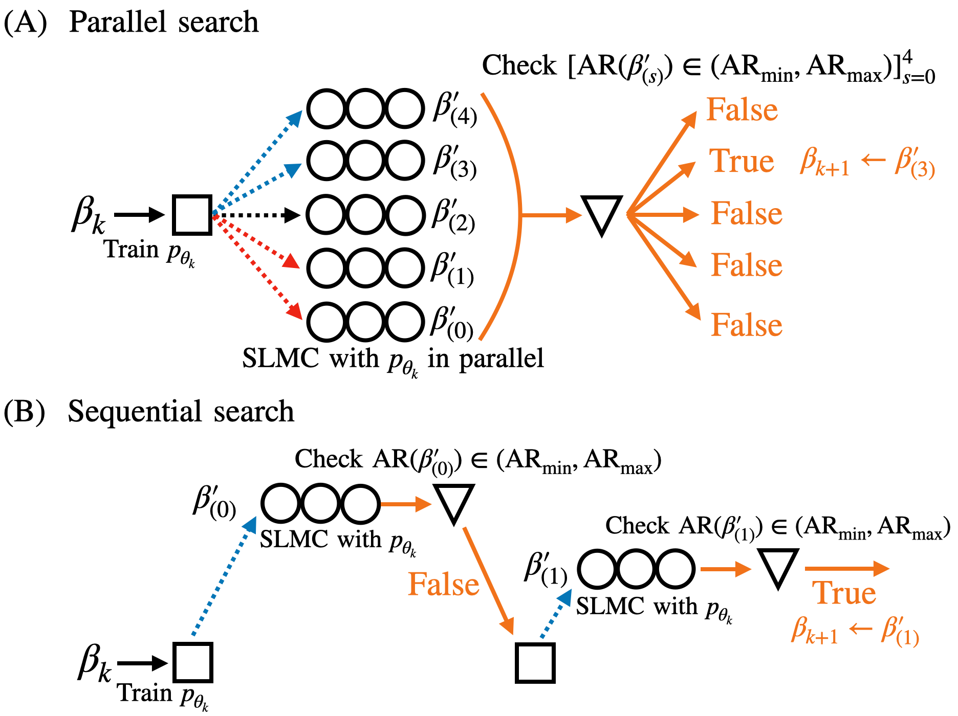
We propose a adaptive annealing, a method to adaptively determine the annealing path while automatically detecting “under-learning”, following the two -search strategies shown in Fig. 2. These two strategies can be used together as the algorithm in Supplementary Material D.2.
Parallel search.
The candidates of are generated in parallel to determine from . The acceptance rates with respect to are then estimated in parallel by a typically small VAE-SLMC simulation with the model , taking advantage of the fact that a VAE can make parallel proposals completely independent of any previous states. After that, the that satisfies is selected as a candidate of . Note that and are lower and upper bounds determined by a user. If there exist multiple candidates, a single candidate is selected according to user-defined criteria (e.g., the smallest is selected).
Sequential search.
First, a candidate is generated and the acceptance rate with respect to is calculated by a typically small SLMC simulation with the model . Then, if is between and , the candidate is accepted as , otherwise, it is rejected and another candidate is generated by
where is a positive constant determined by a user. The new candidate is checked whether it is accepted or not in the same way as described above. This process is repeated until the -th candidate is accepted, and finally is set to .
Note that the proposed methods have an implicit function to detect under-learning of the model and retrain it. If the model is not trained enough, the candidates are all rejected and remains equal to , inducing “retraining” of the model with the same . This is a great advantage of the proposed method over simple scheduling.
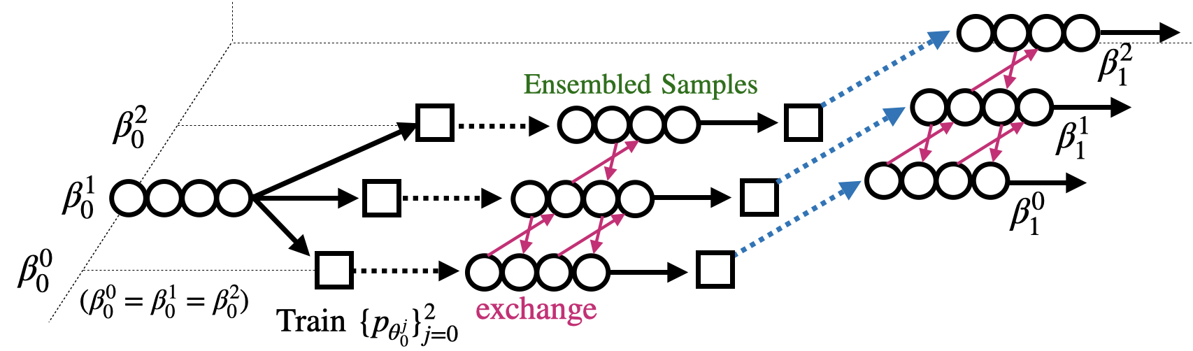
3.3 Parallel Annealing
If the adaptive annealing includes the mode-collapsed model that does not train all modes of the target distribution, it generates samples not covering the all modes on steps larger than . We propose parallel annealing, which superimpose the states of each chain as in ensemble learning and to suppress mode collapse.
We first determine the number of parallel models and set up initial inverse temperature , where the upper/lower index represents the parallel chain/annealing step and then anneal each model in parallel as in the adaptive annealing. The only difference is that when creating the training data in the middle of the annealing, the states of the parallel chain are exchanged according to the following acceptance probabilities,
| (5) |
where is the same acceptance probabilities in the replica exchange Monte Carlo methods (Swendsen & Wang, 1986; Hukushima & Nemoto, 1996). Note that our parallel annealing does not require careful adjustment of the beta intervals so that parallel chains with different inverse temperatures exchange well enough, as in the replica exchange Monte Carlo methods (Swendsen & Wang, 1986; Hukushima & Nemoto, 1996). In parallel annealing, each model is first set to the same condition, , so parallel chains exchange with probability 1, and an ensemble sample is generated from all chains as in ensemble learning. Then, the better models, with a high acceptance rate, have larger intervals from the worse models due to the adaptive annealing. As a result, the better model automatically exchanges with the other better models, and the poor models are rarely exchanged, yielding high-quality ensembled samples. Finally, there is no worry about considering the chains of worse models since we use the best model to reach most quickly. As a result, even if the model fails to learn entire region of the target distribution, the exchange process makes the training data for the model the almost accurate samples. Also, even if there is no mode collapse, utilizing diverse models by the exchange is expected to produce high-quality ensembled training data, leading to better performance; see Supplementary Material D.2 for detailed implementation.
3.4 Self-learning Monte Carlo with VAE
Our VAE-SLMC method adopts a VAE as a proposal model and takes advantage of the VAE’s theoretical properties to calculate acceptance probability efficiently. We can easily compute from Eq. (3) by passing the state through the encoder , and the acceptance probability of the VAE-SLMC becomes
| (6) |
Note that detailed balance holds if Eq. (3) holds, and we validated not a concern in practice by efficient confirmability; see Supplementary Material C.1. The VAE can generate samples at a low cost through the following procedure: The VAE first generates the latent variables, and then generates samples by passing the latent variables through the decoder . A well-trained VAE can make parallel proposals between modes independent of any previous state due to information-rich latent space. Moreover, we briefly confirmed that the method performs better than the methods of (Monroe & Shen, 2022) that also use VAE as a proposal and approximately evaluate the likelihood and of Flow-based model (Albergo et al., 2019) in Supplementary Material E.1. A detailed flow of the VAE-SLMC is shown in Algorithm 1. The model is updated by the “retrain step” with the samples generated by itself. Note that VAE-SLMC is applicable to discrete probability distributions. In addition, A detailed flow of the annealing VAE-SLMC is shown in Algorithm 2.
4 NUMERICAL EXPERIMENT
We start by confirming the effectiveness of the parallel adaptive annealing and the performance on multi-cluster Gaussian mixture distributions. Then, we also validate the performance of the proposed method on real-world application to Bayesian inference of multimodal posterior for spectral analysis; see Supplementary Material C for other discussions and practical applications.
4.1 Experimental condition
We summarize the essential settings for understanding the following results and discussions; the details of all the conditions of the numerical experiments are summarized in the Supplementary Material F.
Abbreviation and proposals.
Table 2 summarizes the experimental conditions and their abbreviations. We experimented with three combinations of our proposed methods for VAE-SLMC, where VAE is set as for simplicity. We practically validated Eq. 3 to ensure the detailed balance according to Supplementary Material C.1. The parameters of MH, MH-EMC, and HMC-EMC are well-tuned. RW and HD in the proposal column of the table denote random walk proposal where is scale factor and Hamilton dynamics (Duane et al., 1987), respectively.
Initial learning.
For the CA-VAE-SLMC and AA-VAE-SLMC, we first train the VAE with 40,000 training data at , which are generated by a local update MCMC method. For each training data set, we trained VAEs until their losses nearly converged.
4.2 Gaussian Mixture
We generalized the two Gaussian mixture proposed in (Woodard et al., 2009) to multi-Gaussian mixture. Specifically, each cluster is assumed to be Gaussian with variance in the dimension, the distance between each cluster is assumed to be equal, and the overall mean is assumed to be . Performance is measured via the root mean squared error (RMSE) defined as the Euclidean distance between the true expected value and its empirical estimate.
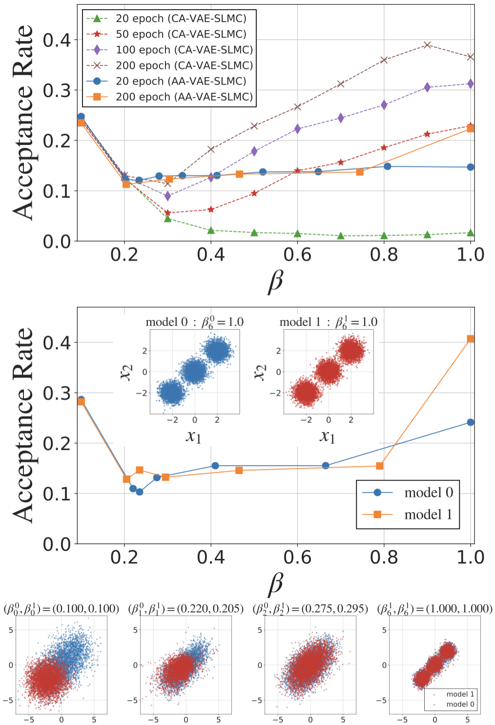
Effectiveness of parallel adaptive annealing.
We compare three methods CA-VAE-SLMC, AA-VAE-SLMC and AA-VAE-ESLMC on three-cluster D Gaussian mixture to confirm the effectiveness of parallel adaptive annealing.
We start by confirming the effectiveness of adaptive annealing by comparing CA-VAE-SLMC and AA-VAE-SLMC, varying the number of learning, i.e., “epoch”, in the middle of annealing (line 5 in Algorithm 2). The CA-VAE-SLMC uses linear annealing path, . In AA-VAE-SLMC, the permissible acceptance rate is between and in parallel search, and the largest of them is selected. Figure 4 (a) shows the relationship between the annealing paths and the acceptance rate corresponding to each beta in the annealing paths. We observe the pre-train effect that CA-VAE-SLMC with 50 epochs works, but for shorter learning, i.e., 20 epochs, the acceptance rate decreases rapidly due to the under-learning of a model. On the other hand, AA-VAE-SLMC with even 20 epochs automatically selects a narrow annealing interval in regions where learning is insufficient and prevents a sudden decrease in acceptance rate. Moreover, the total number of annealing times is 9, which is shorter than CC-VAE-SLMC. It’s interesting to mention that AA-VAE-SLMC with 200 epochs greedily chooses a much shorter annealing path (6 times) due to sufficient learning. These result confirms that the adaptive annealing can automatically detect the under-learning and obtain more efficient annealing paths. Considering the pre-train effect, initially choosing a relatively small number of learning leads to reducing the total number of learning. In fact, the number of learning as a total during annealing of AA-VAE-SLMC with 20 epochs per training is 180 epochs, while AA-VAE-SLMC with 200 epochs per training is 1200 epochs. In addition, we observe that the acceptance rate can be controlled by just adjusting and in Supplementary Material E.2.
Next, we confirm the effectiveness of parallel annealing. For this purpose, we prepared two VAEs of AA-VAE-ESLMC, one of which intentionally learn only one mode at , and the other model that learned all modes at ; see of Figure 4 (c). We observe that parallel annealing recover mode collapse, as shown in Figure 4 (c). Furthermore, Figure 4 (b) shows that adaptive annealing automatically reduces the annealing interval in the region where mode collapse begins to improve. Therefore, parallel annealing with at most two models recovers mode collapse well. The more well-learned models are combined, the earlier the mode collapse is recovered.
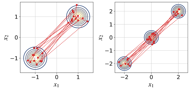
Results of adaptive annealing VAE-SLMC.
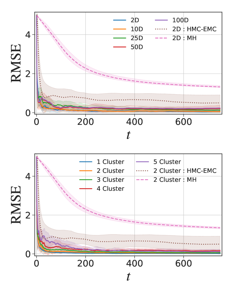
Figure 5 shows the dynamic transitions between the modes by AA-VAE-SLMC with 200 epochs for a two- or three- cluster D Gaussian mixture. Due to the information-rich latent space of the VAE, the proposed method successfully realizes almost equally transitions between clusters at the early stage of the simulation, which is not possible for the local update MCMC method. Figure 6 shows the results when either or is varied and the other is fixed ( or ). We can see that our AA-VAE-SLMC works for these multimodal distributions since the RMSEs drastically decrease compared with MH and HMC-EMC.
4.3 Spectral Analysis
Motivated by (Luengo et al., 2020), we demonstrate real-world Bayesian estimation of a noisy multi-sinusoidal signal (see Supplementary Material E.3 and E.4 for the additional experiments of real-world Bayesian estimation of sensor network localization problems and optimization problems with multiple optimal solutions). The signal is given by
where is a constant term, is a set of amplitudes, are frequencies, are their phases, and is an additive white Gaussian noise. The estimation of the parameters is important in a variety of applications, such as signal processing (Stoica, 1993; So et al., 2005). Here we compute the posterior for given the data by discretizing . Note that the problem is symmetric with respect to hyperplaine and the marginal posterior is multimodal (see Fig. 7). Performance is measured via the relative error of the estimated mean (REM). We apply AA-VAE-SLMC starting from , setting and .

Figure 7 shows our method works for the problem since the REM is rapidly decreased compared with MH-EMC and all modes are covered in the first few transitions, compared with MH-EMC method.
5 RELATED WORK
SLMC methods with a latent generative model have been proposed. First, an SLMC with the restricted Boltzmann machine (RBM) (Huang & Wang, 2017) has been proposed, and the RBM resulted in an efficient global transition. The proposal of the RBM requires the MCMC simulation to be implemented by parallel alternating Gibbs sampling of hidden and visible variables. However, this method can cause problems related to long correlation times (Roussel et al., 2021). An SLMC with a Flow-based model has also been considered (Albergo et al., 2019). The SLMC does not require MCMC and needs to worry about mixing. However, the Flow-based model requires strong restrictions for the networks. Similar to our method is the SLMC with a VAE proposed by (Monroe & Shen, 2022). This method does not require MCMC and has no restriction on the network; however, this method is based on an approximation , whose approximation can lead to a decrease in the acceptance rate, where evaluating the validity of the approximation at a low cost is difficult. Our proposed method can eliminate this approximation by applying the recently derived theoretical analysis of a VAE. They do not provide specific algorithms for situations where obtaining training data is challenging, such as multimodal distributions.
6 CONCLUSION
We have presented parallel adaptive annealing that makes SLMC methods applicable to situations where obtaining accurate training data is difficult. The annealing is based on (i) sequential learning with annealing target distribution to inherit and update the model, (ii) adaptive annealing to automatically detect under-learning, and (iii) parallel annealing to mitigate mode collapse of proposal models. We validate that this combination works on multimodal distribution while automatically detecting and recovering under-learning and mode collapse in the middle of annealing. We also propose the VAE-SLMC method, which utilizes a variational autoencoder (VAE) as the proposal to make efficient parallel proposals by the recently clarified properties of VAE.
We believe that the annealing SLMC methods broaden the applications of the SLMC methods in various fields and the ability to automatically detect under-learning and mode collapse plays an important role in applications of SLMC methods to larger proposal machine learning models and more significantly complicated target distributions. We also expect that continually evolving methods in hardware, software for deep neural network performance and machine learning techniques, including transfer learning and fine-tuning from a various pre-trained models, bring future practical gains for this framework.
To the best of our knowledge, we are the first to consider specific annealing to SLMC methods for multimodal distributions while automatically detecting and recovering under-learning and mode collapse in the middle of annealing. In the future, it will be interesting to see the combination (e.g., small word proposal (Guan et al., 2006)) of gradient-based sampling methods such as variants of HMC (Duane et al., 1987) and Langevin MC Monte Carlo (Roberts & Stramer, 2002) dynamics and our parallel adaptive annealing SLMC methods with latent generative models for much higher dimensional and complex problems.
References
- Albergo et al. (2019) Albergo, M. S., Kanwar, G., and Shanahan, P. E. Flow-based generative models for markov chain monte carlo in lattice field theory. Physical Review D, 100(3):034515, 2019.
- Baumgärtner et al. (2012) Baumgärtner, A., Burkitt, A., Ceperley, D., De Raedt, H., Ferrenberg, A., Heermann, D., Herrmann, H., Landau, D., Levesque, D., von der Linden, W., et al. The Monte Carlo method in condensed matter physics, volume 71. Springer Science & Business Media, 2012.
- Binder et al. (1993) Binder, K., Heermann, D., Roelofs, L., Mallinckrodt, A. J., and McKay, S. Monte carlo simulation in statistical physics. Computers in Physics, 7(2):156–157, 1993.
- Duane et al. (1987) Duane, S., Kennedy, A. D., Pendleton, B. J., and Roweth, D. Hybrid monte carlo. Physics letters B, 195(2):216–222, 1987.
- Foreman-Mackey et al. (2013) Foreman-Mackey, D., Hogg, D. W., Lang, D., and Goodman, J. emcee: the mcmc hammer. Publications of the Astronomical Society of the Pacific, 125(925):306, 2013.
- Gelman et al. (1995) Gelman, A., Carlin, J. B., Stern, H. S., and Rubin, D. B. Bayesian data analysis. Chapman and Hall/CRC, 1995.
- Guan et al. (2006) Guan, Y., Fleißner, R., Joyce, P., and Krone, S. M. Markov chain monte carlo in small worlds. Statistics and computing, 16(2):193–202, 2006.
- Hastings (1970) Hastings, W. K. Monte carlo sampling methods using markov chains and their applications. 1970.
- Higgins et al. (2016) Higgins, I., Matthey, L., Pal, A., Burgess, C., Glorot, X., Botvinick, M., Mohamed, S., and Lerchner, A. beta-vae: Learning basic visual concepts with a constrained variational framework. 2016.
- Himmelblau et al. (2018) Himmelblau, D. M. et al. Applied nonlinear programming. McGraw-Hill, 2018.
- Huang & Wang (2017) Huang, L. and Wang, L. Accelerated monte carlo simulations with restricted boltzmann machines. Physical Review B, 95(3):035105, 2017.
- Hukushima & Nemoto (1996) Hukushima, K. and Nemoto, K. Exchange monte carlo method and application to spin glass simulations. Journal of the Physical Society of Japan, 65(6):1604–1608, 1996.
- Ihler et al. (2004) Ihler, A. T., Fisher III, J. W., Moses, R. L., and Willsky, A. S. Nonparametric belief propagation for self-calibration in sensor networks. In Proceedings of the 3rd international symposium on information processing in sensor networks, pp. 225–233, 2004.
- Inoue et al. (2005) Inoue, M., Hukushima, K., and Okada, M. A pca approach to sourlas code analysis. Progress of Theoretical Physics Supplement, 157:246–249, 2005.
- Inoue et al. (2006) Inoue, M., Hukushima, K., and Okada, M. Analysis method combining monte carlo simulation and principal component analysis–application to sourlas code–. Journal of the Physical Society of Japan, 75(8):084003, 2006.
- Kato et al. (2020) Kato, K., Zhou, J., Sasaki, T., and Nakagawa, A. Rate-distortion optimization guided autoencoder for isometric embedding in Euclidean latent space. In International Conference on Machine Learning, pp. 5166–5176. PMLR, 2020.
- Kingma & Welling (2013) Kingma, D. P. and Welling, M. Auto-encoding variational bayes. arXiv preprint arXiv:1312.6114, 2013.
- Kirkpatrick et al. (1983) Kirkpatrick, S., Gelatt Jr, C. D., and Vecchi, M. P. Optimization by simulated annealing. science, 220(4598):671–680, 1983.
- Kiwata (2019) Kiwata, H. Deriving the order parameters of a spin-glass model using principal component analysis. Physical Review E, 99(6):063304, 2019.
- Levy et al. (2017) Levy, D., Hoffman, M. D., and Sohl-Dickstein, J. Generalizing hamiltonian monte carlo with neural networks. arXiv preprint arXiv:1711.09268, 2017.
- Liu et al. (2017) Liu, J., Qi, Y., Meng, Z. Y., and Fu, L. Self-learning monte carlo method. Physical Review B, 95(4):041101, 2017.
- Luengo et al. (2020) Luengo, D., Martino, L., Bugallo, M., Elvira, V., and Särkkä, S. A survey of monte carlo methods for parameter estimation. EURASIP Journal on Advances in Signal Processing, 2020(1):1–62, 2020.
- Manly (2018) Manly, B. F. Randomization, Bootstrap and Monte Carlo Methods in Biology: Texts in Statistical Science. chapman and hall/CRC, 2018.
- Martin et al. (2011) Martin, A. D., Quinn, K. M., and Park, J. H. Mcmcpack: Markov chain monte carlo in r. 2011.
- Monroe & Shen (2022) Monroe, J. I. and Shen, V. K. Learning efficient, collective monte carlo moves with variational autoencoders. Journal of Chemical Theory and Computation, 2022.
- Nagata & Watanabe (2008) Nagata, K. and Watanabe, S. Asymptotic behavior of exchange ratio in exchange monte carlo method. Neural Networks, 21(7):980–988, 2008.
- Nakagawa et al. (2021) Nakagawa, A., Kato, K., and Suzuki, T. Quantitative understanding of vae as a non-linearly scaled isometric embedding. In International Conference on Machine Learning, pp. 7916–7926. PMLR, 2021.
- Neal et al. (2011) Neal, R. M. et al. Mcmc using hamiltonian dynamics. Handbook of markov chain monte carlo, 2(11):2, 2011.
- Rastrigin (1974) Rastrigin, L. A. Systems of extremal control. Nauka, 1974.
- Roberts & Stramer (2002) Roberts, G. O. and Stramer, O. Langevin diffusions and metropolis-hastings algorithms. Methodology and computing in applied probability, 4(4):337–357, 2002.
- Rolinek et al. (2019) Rolinek, M., Zietlow, D., and Martius, G. Variational autoencoders pursue pca directions (by accident). In Proceedings of the IEEE/CVF Conference on Computer Vision and Pattern Recognition, pp. 12406–12415, 2019.
- Roussel et al. (2021) Roussel, C., Cocco, S., and Monasson, R. Barriers and dynamical paths in alternating gibbs sampling of restricted boltzmann machines. Physical Review E, 104(3):034109, 2021.
- Shen et al. (2018) Shen, H., Liu, J., and Fu, L. Self-learning monte carlo with deep neural networks. Physical Review B, 97(20):205140, 2018.
- Shlens (2014) Shlens, J. A tutorial on principal component analysis. arXiv preprint arXiv:1404.1100, 2014.
- Silagadze (2007) Silagadze, Z. Finding two-dimensional peaks. physics of Particles and Nuclei Letters, 4(1):73–80, 2007.
- So et al. (2005) So, H.-C., Chan, K. W., Chan, Y. T., and Ho, K. Linear prediction approach for efficient frequency estimation of multiple real sinusoids: algorithms and analyses. IEEE Transactions on Signal Processing, 53(7):2290–2305, 2005.
- Sohl-Dickstein et al. (2014) Sohl-Dickstein, J., Mudigonda, M., and DeWeese, M. Hamiltonian monte carlo without detailed balance. In International Conference on Machine Learning, pp. 719–726. PMLR, 2014.
- Stoica (1993) Stoica, P. List of references on spectral line analysis. Signal Processing, 31(3):329–340, 1993.
- Swendsen & Wang (1986) Swendsen, R. H. and Wang, J.-S. Replica monte carlo simulation of spin-glasses. Physical review letters, 57(21):2607, 1986.
- Tanaka & Tomiya (2017) Tanaka, A. and Tomiya, A. Towards reduction of autocorrelation in hmc by machine learning. arXiv preprint arXiv:1712.03893, 2017.
- Wang (2016) Wang, L. Discovering phase transitions with unsupervised learning. Physical Review B, 94(19):195105, 2016.
- Woodard et al. (2009) Woodard, D., Schmidler, S., and Huber, M. Sufficient conditions for torpid mixing of parallel and simulated tempering. Electronic Journal of Probability, 14:780–804, 2009.
- Xu et al. (2017) Xu, X. Y., Qi, Y., Liu, J., Fu, L., and Meng, Z. Y. Self-learning quantum monte carlo method in interacting fermion systems. Physical Review B, 96(4):041119, 2017.
Appendix A OVERVIEW
This supplementary material provides extended explanations, implementation details, and additional results for the paper “Toward Unlimited Self-Learning MCMC with Parallel Adaptive Annealing”.
Appendix B PROOF SKETCH
In this section, we show a brief sketch of Eq. 3 derivation in main text as a summary of previous works from Rolinek et al. (2019); Nakagawa et al. (2021); Kato et al. (2020). Here, we assume that the dimension of the data manifold is , and this manifold is embedded in the -dimensional input space.
First, we explain the case of , i.e., the dimension of the data manifold is the same as the dimension of the input space for simplicity. In this case, we need to set . Here, Kato et al. (2020) show that the loss function in Eq. (2) can be approximated as follows:
| (9) |
where denote a metric tensor from if holds. Kato et al. (2020) further derived the optimal condition of Eq. (9) as follows:
| (10) |
where denotes the Kronecker delta. They called the quantitative orthogonal property of Eq. (10) implicit isometricity. In the case , the reconstruction loss becomes the sum of squared errors (SSE) and the metric tensor becomes an identity matrix . From Eq. (10), we can derive the Jacobian determinant between and as follows:
| (11) |
Thus the probability of sample can be derived from the prior and Jacobian determinant as follows:
| (12) |
Second, we explain the case of , i.e., the dimension of the data manifold is less than the dimension of the input space. In this case, the value of the probability density cannot be defined in the -dimensional input space. Instead, we need to measure the probability density in the manifold space with the dimension . The following show an example. Assume a 2-dimensional square plane manifold with edge length L in 3-dimensional space. In the 3-dimensional space, the probability density of the point on the square plane manifold is infinite, and the probability density of the point out of the square plane manifold is zero. By contrast, if we focus on the 2-dimensional manifold only, we can derive the probability density of the points on the square plane manifold as .
In this case, Rolinek et al. (2019) show that the following “polarized regime” is typically observed when a VAE is trained:
Definition B.1.
We say that parameters , induce a “polarized regime” if the latent space can be partitioned to and (active and passive set) such that
-
(a)
, ,
-
(b)
, , , .
Rolinek et al. (2019) showed that polarized regime is typically observed very early in the training in the multiple data sets such as dSprites, MNIST, and Fashion MNIST. Nakagawa et al. (2021) also reported that the polarized regime is observed in CelebA dataset. Here, and are regarded as subspaces of the data manifold which a VAE learned and out of the manifold, respectively. Thus, Eq. (3) can be expanded using polarized regime (b) under the optimal conditions as follows:
| (13) | |||||
since the second product term regarding in the second equation is constant. Here, in Eq. (13) can be considered to be proportional to the probability density on the data manifold space from the last equation of Eq. (13). Thus, , i.e., the dimension of , can be be reduced down to , which will be corresponding to .
Note that Kato et al. (2020) introduced an isometric variational autoencoder called RaDOGAGA and showed the precise and mathematical derivation of the probability density when . Since the work of Nakagawa et al. (2021) which show Eqs. (9)-(12) is an expansion of Kato et al. (2020), Eq. 13 can be mathematically derived in the same manner.
Appendix C EXTENDED EXPLANATIONS OF VAE’s IMPLICIT ISOMETRICITY
In this section, we show how to check the consistency of the VAE’s implicit isometricity shown in the paper and how to efficiently analyze the properties of probability distributions from the obtained samples using the implicit isometricity.
C.1 Checking Isometricity of the VAE
This section shows how to check whether a VAE acquires the isometricity. In the following discussion, we assume that the SSE metric is used as a reconstruction loss of the VAE objective. From Eq. (10) and , a following property
| (14) |
holds in each latent dimension . Eq. (14) can be numerically estimated as
| (15) |
where is a trained VAE decoder, is an infinitesimal constant for numerical differentiation, and is a one-hot vector , in which only the -th dimensional component is and the others are . We define the isometric factor for each latent dimension as
| (16) |
where denote the average value over the generated 100,000 samples from . If the isometric factor is close to , the probability can be correctly estimated by using Eq. (3) in the main document. Note that the orthogonality holds as shown in (Nakagawa et al., 2021; Rolinek et al., 2019).
Table 2 shows the isometric factor of each dimension of the VAE latent variable in a descending order of the importance calculated by Eq. (17). in Eq. (16) is set to . GMM- show Gaussian Mixtures () with clusters used in Sec. 4.1 in the main text. ICG is Ill-Conditional Gaussian () explained in Section D.2. For ICG, top 10-dimensional values from 100 dimensions are listed in the table. BANANA (), SCG (), and RW () denote banana-shaped density, strongly correlated Gaussian, and rough well distributions, respectively, as explained in Sec. D.2. See Sec. F for details of the experiment conditions. As shown in this table, the isometric factors for each dimension in our experiments are very close to 1.0, showing the proposal probability can be correctly estimated from Eq. (3) in the main document.
| Latent dim. | GMM-2 | GMM-3 | GMM-4 | GMM-5 | ICG | BANANA | SCG | RW |
|---|---|---|---|---|---|---|---|---|
| 1 | 0.974 | 0.978 | 0.996 | 0.987 | 1.009 | 1.009 | 1.000 | 0.999 |
| 2 | 0.986 | 0.987 | 0.990 | 0.990 | 1.013 | 0.993 | 1.003 | 1.000 |
| 3 | 0.990 | 0.987 | 0.990 | 0.992 | 1.013 | |||
| 4 | 0.987 | 0.991 | 0.999 | 0.994 | 1.012 | |||
| 5 | 0.993 | 0.993 | 0.992 | 0.996 | 1.000 | |||
| 6 | 0.992 | 0.993 | 1.000 | 0.992 | 1.019 | |||
| 7 | 0.992 | 0.995 | 0.996 | 0.991 | 1.014 | |||
| 8 | 1.001 | 0.992 | 1.000 | 0.990 | 1.013 | |||
| 9 | 0.999 | 1.004 | 1.001 | 0.995 | 1.004 | |||
| 10 | 1.002 | 1.004 | 0.993 | 0.997 | 1.025 |
C.2 Understanding the Structure of Probability Distributions
By using the properties of VAE, the structure of probability distributions can be analyzed at low cost. In Bayesian statistics and other probabilistic inference, principal component analysis (PCA) (Shlens, 2014) of the samples generated by a sampling method such as MCMC methods is sometimes performed to understand the structure of probability distribution (Inoue et al., 2005, 2006; Wang, 2016; Kiwata, 2019). However, the computational cost for calculating eigenvalues in PCA is , where is the data dimension and is the number of samples generated by an MCMC method. However, by using the VAE obtained by VAE-SLMC, a low-dimensional compression similar to PCA is possible just by encoding and decoding the samples with a cost of , where is a computational cost of a VAE’s encoder. The importance of each latent dimension in the latent space can be evaluated (Nakagawa et al., 2021) as
| (17) |
We substitute for the empirical mean of samples and encoded variance can be obtained by passing samples through encoder-decoder.
Appendix D ALGORITHM DETAILS
In this section, we describe the implementation details of the proposed VAE-SLMC with adaptive annealing and parallel annealing methods.
D.1 Summary of the Proposed VAE-SLMC Methods
Here, we summarize the variation of the proposed VAE-ALMC methods. Table 3 lists all the combinations of the proposed method with the adaptive annealing technique (in Sec. 3.3 and Algorithms 3 and 4) and the parallel annealing exchange technique (in Sec. 3.4 and Algorithms 5 and 6). The abbreviations of the algorithms (CA-VAE-SLMC, AA-VAE-SLMC, and AA-VAE-ESLMC) used in the experiments are also described. “CA-” means constant annealing, which is a method without adaptive annealing.
| VAE-SLMC | Annealing | Adaptive annealing | Parallel annealing exchange | |
|---|---|---|---|---|
| (Sec. 3.1) | (Sec. 3.2) | (Sec. 3.3) | (Sec. 3.4) | |
| Method | (Alg. 1) | (Alg. 2) | (Alg. 3 and 4) | (Alg. 5 and 6) |
| Naïve VAE-SLMC | ||||
| CA-VAE-SLMC | ||||
| AA-VAE-SLMC | ||||
| AA-VAE-ESLMC |
D.2 Adaptive Annealing VAE-SLMC
Algorithm 3 illustrates the steps of adaptive annealing VAE-SLMC (AA-VAE-SLMC) explained in Sec. 3.3 of the main text. The details the input of Alogorithm 3 are as follows:
-
•
A target distribution : A probability distribution from which a user wishes to sample, where the normalizing factor is not necessary to compute acceptance probability.
-
•
An initial : The inverse temperature where the annealing starts, where should be set so that the distribution is easily explorable even with a local update MCMC method.
-
•
Training data : Training data used to train the initial model .
-
•
An initial model : A model trained with the training data .
-
•
An initial distribution : An initial distribution of VAE-SLMC during annealing. In simulated annealing, it is necessary to simulate the probability distribution with the final state of the simulation of the probability distribution as the initial value because the transition between modes becomes more difficult as the inverse temperature is large. However, VAE-SLMC works for arbitrary initial distributions because the proposal is independent of previous states, and transitions between modes are easy. Therefore, the algorithm uses the same initial distribution for all without loss of generality.
In all the numerical experiments, we set in order not to perform the retraining steps in the VAE-SLMC in from Algorithm 1.
In Line 3 of Algorithm 3, is adaptively determined by Algorithm 4, whose inputs are detailed as follows:
-
•
: A current value of .
-
•
, : Upper and lower bounds for the acceptance rate of the VAE-SLMC at each annealing step. The upper and lower bounds are the values determined by a user according to the acceptance rate sought at the end of the annealing . For a typical behavior of the lower and upper bounds of the adaptive annealing VAE-SLMC, please refer to Sec. E.2.
-
•
: A parameter used to update the candidates in a sequential search step.
-
•
: An initial sequence of candidates . They consist of the input and smaller and larger values around with a user-defined granularity, e.g., an equal interval or a logarithmically equal interval.
-
•
: The maximum number of iterations for sequential search.
-
•
: The number of the Monte Carlo steps in VAE-SLMC used to estimate acceptance rates of the candidates .
The followings are additional notes with respect to Algorithm 4:
Parallel calculation of acceptance rates.
In order to calculate the acceptance rates of candidates in Line 2 by a local update MCMC method, it is necessary to calculate the acceptance rate by times local update MCMC simulations. Computation of the acceptance rates in Line 2 can be executed in parallel since SLMC proposes candidates independent of the previous state. In other words, the overhead of calculating the acceptance rates for candidates by using SLMC only changes the number of calculating acceptance rates from to for each step of VAE-SLMC.
Selection from candidates.
In Line 5, if there are multiple s that satisfy the conditions, you can select according to arbitrary rules. For example, if you select the largest among all the s satisfying the condition, the number of annealing steps will be small, but the acceptance rate will be about the lower bound. On the other hand, if you select the smallest among all the s satisfying the conditions, the number of annealing steps will be larger, but the acceptance rate will be about the upper bound.
D.3 Parallel Annealing Exchange VAE-SLMC
Algorithm 5 illustrates the steps of parallel annealing exchange VAE-SLMC explained in Sec. 3.4 of the main text. The details the input of Algorithm 5 are as follows:
-
•
A target distribution : A probability distribution from which a user wishes to sample, where the normalizing factor is not necessary to compute acceptance probability.
-
•
A -sequence : A set of s to determine the annealing schedules for all the parallel chains. and indices represent the parallel chains and the annealing steps, independently.
-
•
An initial model : A model trained with the training data from by a local update EMC method.
-
•
Training data : Training data used to train the initial model .
-
•
An initial distribution : An initial distribution of VAE-ESLMC during annealing. We use the same initial distribution in the annealing for the same reasons as described in Sec. D.2.
In Line 4 of Algorithm 5, samples are generated by VAE-ESLMC described in Algorithm 6, which uses the same exchange process as the replica exchange Monte Carlo method (Swendsen & Wang, 1986; Hukushima & Nemoto, 1996). For all parallel chains, the exchange probability is defined as
| (18) |
The same “retrain” step as in VAE-SLMC can also be incorporated into the VAE-ESLMC. However, retraining is not performed in all numerical experiment (i.e., ).
Appendix E ADDITIONAL RESULTS
In this section, we report additional results omitted from the main text because of limited space.
E.1 Comparing VAEs and Flow based model
This section compares our proposed VAE-SLMC with other VAE-SLMC proposed in Monroe & Shen (2022) and Flow-SLMC proposed in Albergo et al. (2019). We briefly describe the VAE-based method proposed in Monroe & Shen (2022). Although Monroe & Shen (2022) use the prior and the posterior constructed by Flow-based model, we consider the simple prior and posterior case in Sec 2.3 for simplicity. The basic idea of Monroe & Shen (2022) is that a well-trained VAE may reach the case that the true posterior and variational posterior coincide, i.e., , and approximates the likelihood function as
Next, we describe the Flow-based model (RealNVP) used in following comparison. We use an affine coupling layer consisting of a three-layer fully-connected neural network with leaky rectified linear activations, refered in Albergo et al. (2019). On the other hand, The VAE was the same VAE commonly used in the numerical experiments in this paper; see Supplementary Material F.3 for the details of the VAE.
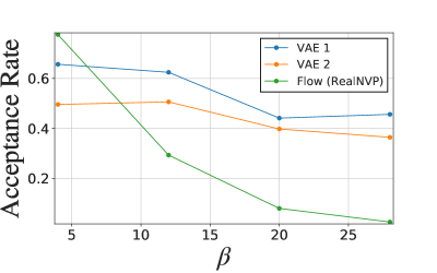
The details of the number of parameters for each model are summarized in Table 4. Each model was trained until the loss nearly converged. Figure 9 shows the relationship between each dimension of target distribution and the acceptance rate to compare the differences between the models and the methods (VAE 1: our proposed method, VAE 2: method in Monroe & Shen (2022)) on cluster Gaussian mixture at . We observe that our method obtains the highest acceptance rate, even in a limited setting. An exhaustive search is in the future work.
| Dimension | 4 | 12 | 20 | 28 |
|---|---|---|---|---|
| Number of VAE parameters | 263,244 | 269,924 | 276,604 | 283,284 |
| Number of Flow parameters | 270,352 | 282,672 | 294,992 | 307,312 |
E.2 Dependency of in Algorithm 3
Figure 10 shows the dependency of the lower bound in AA-VAE-SLMC on the annealing and the acceptance rate denoted on the colorbar after -th annealing step, and the RMSEs after -th Monte Carlo step in three-cluster D Gaussian, which are the same settings used in the main text Sec. except for lower bound . This result confirms that the acceptance rate falls appropriately between the upper bound and lower bounds.
From these results, a large value of requires a long number of annealing to reach , while a small value of results in a small number of annealing to reach . Specifically, when , 11 times of annealing () are required to reach , but when , only 3 times of annealing () are required. We also find that for any given , the RMSE decreases as same, indicating that the algorithm works for any given . Furthermore, when is between 0.1 and 0.5, the last beta intervals become smaller because , and the acceptance rates increase rapidly. These result suggests that our adaptive annealing control the acceptance rate in the middle of annealing, which is effective to set to a low value, reduce the number of the annealing.

E.3 Sensor Network Localization
In this section, we examine the results of AA-VAE-SLMC applied to the problem to estimate the location of a sensor network by Bayesian estimation. This problem is typically a multimodal posterior distribution with multiple modes; see Supplementary Material Sec. F for details of parameter settings of the AA-VAE-SLMC. Specifically, we follow the experimental setup by (Ihler et al., 2004) and assume that sensors have two-dimensional locations denoted by and exist in a two-dimensional plane. The distance between a pair of sensors is observed with probability , and the distance follows , including Gaussian noise. Given a set of observations and a prior (uniform distribution) of , a typical task is to infer all sensor positions from the posterior distribution. We set (), , , and add three sensors with known positions. The positions of eight sensors form a -dimensional multimodal distribution. This distribution is difficult for a local updated MCMC method to visit all the modes, and a large bias is introduced to the obtained samples. Convergence is evaluated using the relative error of the estimated mean (REM) in all dimensions. The REM is a summary of the error in approximating the expected value of a variable across all dimensions, which is computed as
| (19) |
where and denote the sampling average of the -th variable at time . Moreover, is the mean of the -th variable of the target probability distribution. We first train the VAE with 40, 000 training data at , which are generated using a local updated MCMC method with the acceptance rate tuned to almost in a range between 0.2 and 0.3. AA-VAE-SLMC start from and, we set , , ; adaptive from at each proposal step. The left side of Fig. 11 shows the dynamics of the REM and the right side of Fig. 11 shows known and unknown sensor positions and generated samples by AA-VAE-SLMC on two-dimensional planar.
The REM rapidly decreases for samples with a fast transition between multiple modes and small autocorrelation (see Sec. F.5). The figure on the left shows that AA-VAE-SLMC has a much more rapidly decreasing REM than MH-EMC, which suggests that the VAE obtained by annealing is proposing between modes at high speed, producing samples with much smaller autocorrelations. The figure on the right shows that multiple modes of the posterior distribution can be sampled precisely centered on the true position of the unknown sensor.

E.4 Optimization Problems
By considering the cost function to minimize as a negative log-likelihood and annealing to sufficiently large , the optimization problem can be solved in the same way as simulated annealing (Kirkpatrick et al., 1983). Here, we demonstrate our method is extremely effective in searching for multiple globally optimal solutions. Specifically, we confirm the behavior of AA-VAE-SLMC on the following Himmelblau function (Himmelblau et al., 2018):
| (20) |
It is one of the famous optimization problems with the following global optima:
We use AA-VAE-SLMC method starting from to and set and ;
Figure 12 (Left) shows that the generated samples consist only of states near the optimal solution and that the four optimal values are generated with almost equal probability, whose global transition is effective complex optimization problmes. The acceptance rate is about , and the RMSE between the estimated value of the function and the true optimal value of the function is across 10 chain average and standard deviation up to 50,000 iterations.
We also validate the performance of AA-VAE-SLMC for other optimization problems in addition to the Himmelblau function. We use three standard benchmark test functions: Rastrigin function (Rastrigin, 1974), and Styblinski–Tang function (Silagadze, 2007). See Supplementary Material Sec. F for details of the parameter setting for AA-VAE-SLMC.
-
•
Rastrigin function: A function that has a global optimal solution at the origin, where the function value is zero, defined by
subject to . The global minimum is located at , .
-
•
Styblinski–Tang function: A function with three local solutions and one globally optimal solution in the two-dimensional case:
subject to . The global minimum is located at
Table 5 shows that the RMSE between the objective function estimated by an MCMC method and the true optimal value:
| (21) |
where denotes the average cost function estimated by 50,000 Monte Carlo steps, under the number of annealing steps , an initial beta , and a final beta . The smaller the , the closer the generated samples are to the global optimal, meaning that the optimization problem is solved more accurately. As can be seen from Table 5, the RMSEa are very small in all situations, indicating that the AA-VAE-SLMC can solve the optimization problems even for problems with multiple local optimal and somewhat high dimensionality. Figure 12 shows that snapshots of the transitions of AA-VAE-SLMC for each problem. For the problems with multiple global optimal solutions, the samples should be generated from the global optimal with almost equal probability. In the case of a single global optimal, it is also desirable that the samples be generated in the vicinity of a single global optimal solution, skipping over the local optimal. As can be seen from the figure, for the Himmelblau function with four globally optimal solutions, the samples are generated on the four global optimal with almost equal probability. For the Rastrigin and Styblinski–Tang functions, the samples are generated immediately in the vicinity of the global optimal from the initial state. These global transitions are achieved by the information-rich latent space of well-trained VAE. Such a global transition is not feasible for simulated annealing using the local update and may be an efficient optimization method.
| Target | in Eq. (21) | Annealing steps | Initial beta | Final beta |
|---|---|---|---|---|
| Rastrigin (D) | ||||
| Rastrigin (D) | ||||
| Styblinski–Tang (D) | ||||
| Styblinski–Tang (D) |

E.5 Experimets of Naïve VAE-SLMC
In this section, we show that even the naïve VAE-SLMC can generate samples more efficiently than HMC, the most common method for continuous probability distributions when good training data can be obtained. We evaluate the performance of the naïve VAE-SLMC which uses only Algorithm 1, i.e., without annealing, on the following toy test distributions:
-
•
Ill-conditioned Gaussian (ICG): A 100-dimensional multivariate normal distribution with mean and variance . Eigenvalues of range from to and eigenvectors are chosen in a random orthonormal basis.
-
•
Strongly correlated Gaussian (SCG): A diagonal 2-dimensional normal distribution with variance rotated by . This is an extreme version of the example by (Neal et al., 2011).
-
•
Banana-shaped density (BANANA): A 2-dimensional probability distribution as
This distribution has a strong ridge-like geometrical structure that is difficult for HMC (Duane et al., 1987) to understand its structure.
-
•
Rough well density (RW): A distribution similar to the example by (Sohl-Dickstein et al., 2014), for a given ,
For a small , the distribution itself does not change much, but the surface is perturbed by high-frequency tines oscillating between and . In our numerical experiments, we set .
For each of them, we compare the naïve VAE-SLMC with Hamilton Monte Carlo (HMC) (Duane et al., 1987) which fix leapfrog steps and use well-tuned step size. We also set to train a VAE. The samples used as training data were generated by well-tuned HMC and spaced long enough to be almost independent samples; see Supplementary Materials Sec. F.4 for details of parameters of HMC. In this numerical experiment, the performance of VAE-SLMC is evaluated by ESS, which is commonly used in HMC evaluations (Levy et al., 2017), instead of RMSE. Specifically, we measured performance via the mean across runs of the minimum effective sample size (ESS) across dimensions and the 1st and 2nd order moments, motivated by (Levy et al., 2017); see Supplementary Materials Sec. F.5 for details of definition and meaning. Table 6 summarizes the results for the distributions. The naïve VAE-SLMC performs well in the experiments. This result indicates that MCMC can be significantly accelerated if a good sequence of samples is obtained by some method.
| Target | HMC | Naïve VAE-SLMC |
|---|---|---|
| Ill-conditioned Gaussian (D) | ||
| Strongly correlated Gaussian (D) | ||
| Banana-shaped density (D) | ||
| Rough well density (D) |
Appendix F EXPERIMENT DETAILS
F.1 Model Details
The followings are additional details of the models used in the experiments of the main paper.
Gaussian Mixture.
In Sec. 4.1 of the main text, we first define , and consider the following Gaussian mixture models:
-
•
-cluster gaussian mixture:
-
•
-cluster Gaussian mixture:
-
•
-cluster Gaussian mixture:
-
•
-cluster Gaussian mixture:
Spectral Analysis.
In Sec. 4.2 of the main text, we obtain the data by discretizing with a period :
where , and we define the following posterior to estimate frequencies :
where denotes a indicator function such that if and if , which is based on the periodicity outside of . Furthermore, for the sake of simplicity, let assume that and are known, we set , , .
F.2 Experimental Conditions for the Annealing VAE-SLMC Methods
We describe the specific hyperparameters of the annealing of CA-VAE-SLMC, AA-VAE-SLMC, CA-VAE-ESLMC, and AA-VAE-ESLMC for each experiment in Table 7. The algorithms for each method explained in Table 3 are invoked with these hyperparameters. In all the numerical experiments, retrain step in VAE-SLMC (Algorithm 1) and VAE-ESLMC (Algorithm 6) was not performed for each annealing (i.e., ). We did not perform parallel search in Algorithm 4 for simplicity (i.e., ), and sequential search was performed from to input . was set to the value obtained by dividing the interval between and input by .
| Experiment | Method | Epoch | ||||||
|---|---|---|---|---|---|---|---|---|
| Gaussian Mixture | CA-VAE-SLMC | |||||||
| AA-VAE-SLMC | ||||||||
| AA-VAE-ESLMC | ||||||||
| Spectral Analysis | AA-VAE-SLMC | |||||||
| Sensor Problems | AA-VAE-SLMC | |||||||
| Optimization Problems | AA-VAE-SLMC |
F.3 Conditions for Training the VAE in VAE-SLMC
In this section, we summarize the parameter settings for model assignment and learning for VAE.
VAE configulations.
We define as a fully-connected layer with input dimension , output dimension , and activate function , and and as a input dimension and a latent dimension, respectively. We used the same network and set for all numerical experiments in Sec. 4 and Sec. E. The encoder is composed of ------ and the decoder is ------.
Training hyperparameters.
Table 8 summarizes the training parameters other than the network. In all numerical experiments, we use an Adam optimizer and the sum of squared errors (SSE) for the objective function.
F.4 Details of the Replica Exchange Monte Carlo (EMC) and Metropolis–Hastings (MH) Methods in Table 1.
In this section, we show each method and its parameters used in the experiments. For the Metropolis–Hastings (MH) method, we used the proposal with Gaussian distribution and adjusted the scale parameter so that the acceptance rate is between 0.15 and 0.25. In the replica exchange Monte Carlo (EMC) method, the interval of the inverse temperatures is set so that the exchange acceptance rate between replicas is about 0.3 with equal probability by following (Nagata & Watanabe, 2008). When the kernel of each replica is , we adjusted scale parameter so that the acceptance rate is between 0.15 and 0.25. When the kernel of each replica is Hamilton Monte Carlo (HMC) kernel, the number of steps is fixed to 5, and the step size is set so that the acceptance rate is about between 0.4 and 0.6. The EMC method with HMC was implemented using the TensorFlow Probability’s tfp.mcmc.ReplicaExchangeMC111https://www.tensorflow.org/probability/api_docs/python/tfp/mcmc/ReplicaExchangeMC implementation.
F.5 Detail of Metrics
This section provides the details and purposes of the three metrics used in our experiments.
Root-mean-square error (RMSE).
RMSE is defined as the Euclidean distance between the true expected value and its estimate:
| (22) |
where denotes the sampling average of the -th dimension of the variable at Monte Carlo step , and is the mean of the -th dimension of the variable mathematically derived from the target distribution. A rapid decrease of means a faster convergence to a mean of the target probability distribution. When all modes of the target distribution cannot be accurately explored, RMSE does not converge to zero.
RMSE is helpful to evaluate whether the samples are biased or not. Furthermore, the convergence rate takes longer if the samples cannot efficiently move between modes. Therefore, we used RMSE in Gaussian mixture experiments in main text Sec. 4.1 to ensure that annealing VAE-SLMC efficiently moves between modes and generates unbiased samples.
Relative error (REM).
A summary of the error in approximating the expected value of a variable across all dimensions computed by
| (23) |
where and are the same as in RMSE above. REM is divided by the true mean to eliminate dependence on the scale for each dimension . A rapid decrease of means a faster convergence to a mean of the target probability distribution.
REM is also helpful to evaluate the bias of samples like RMSE. Since REM is scale-invariant by considering the normalization for each dimensional component of sample space, we used REM for the spectral problem in main text Sec. 4.2 and sensor problems in Sec. E.3 where the scales of each dimension are different.
Effective sample size (ESS).
ESS is a common measure to evaluate efficiency of sampling algorithms. The ESS represents the estimated number of iid samples generated. When measuring ESS in higher dimensions, it is common to consider ESS for each dimension. For a sequence of samples , the effective sample size (ESS) was computed as
| (24) |
where is the stopping time. is an estimate of the lag- autocorrelations of the Markov chain:
| (25) |
The ESS is calculated by using TensorFlow Probability’s tfp.mcmc.effective_sample_size222https://www.tensorflow.org/probability/api_docs/python/tfp/mcmc/effective_sample_size implementation. If an MCMC simulation generates completely independent samples, then . We report the mean across 10 runs of minimum ESS across dimensions and the 1st and the 2nd moments.
ESS is a helpful measure to quantify the correlation between samples and to see the number of samples that are effectively independent and is the most commonly used evaluation measure in Bayesian estimation for gradient-based MCMCs such as HMC. On the other hand, it is difficult for ESS to capture whether the transition between modes is efficient visually. Therefore, in the performance evaluation of Naïve VAE-SLMC in Sec. E.5, we use ESS as the metric because it is not a particularly multimodal distribution, and we wanted to confirm its superiority over HMC for distribution families that HMC is not good at.