SCOOP: Self-Supervised Correspondence and Optimization-Based Scene Flow

Abstract

Scene flow estimation is a long-standing problem in computer vision, where the goal is to find the 3D motion of a scene from its consecutive observations. Recently, there have been efforts to compute the scene flow from 3D point clouds. A common approach is to train a regression model that consumes source and target point clouds and outputs the per-point translation vector. An alternative is to learn point matches between the point clouds concurrently with regressing a refinement of the initial correspondence flow. In both cases, the learning task is very challenging since the flow regression is done in the free 3D space, and a typical solution is to resort to a large annotated synthetic dataset.

We introduce SCOOP, a new method for scene flow estimation that can be learned on a small amount of data without employing ground-truth flow supervision. In contrast to previous work, we train a pure correspondence model focused on learning point feature representation and initialize the flow as the difference between a source point and its softly corresponding target point. Then, in the run-time phase, we directly optimize a flow refinement component with a self-supervised objective, which leads to a coherent and accurate flow field between the point clouds. Experiments on widespread datasets demonstrate the performance gains achieved by our method compared to existing leading techniques while using a fraction of the training data. Our code is publicly available.

1 Introduction

Scene flow estimation [33] is a fundamental problem in computer vision with various use-cases, such as autonomous driving, scene parsing, pose estimation, and object tracking, to name a few. Given two consecutive observations of a 3D scene, the aim is to compute the dynamics of the scene between the observations. Scene flow prediction based on 2D images has been thoroughly investigated in the literature [39, 38, 34, 23, 21]. However, in light of the recent proliferation of 3D sensors, such as LiDAR, there is a surge of interest in scene flow methods that operate directly on the 3D data [20, 11, 25, 41, 17].

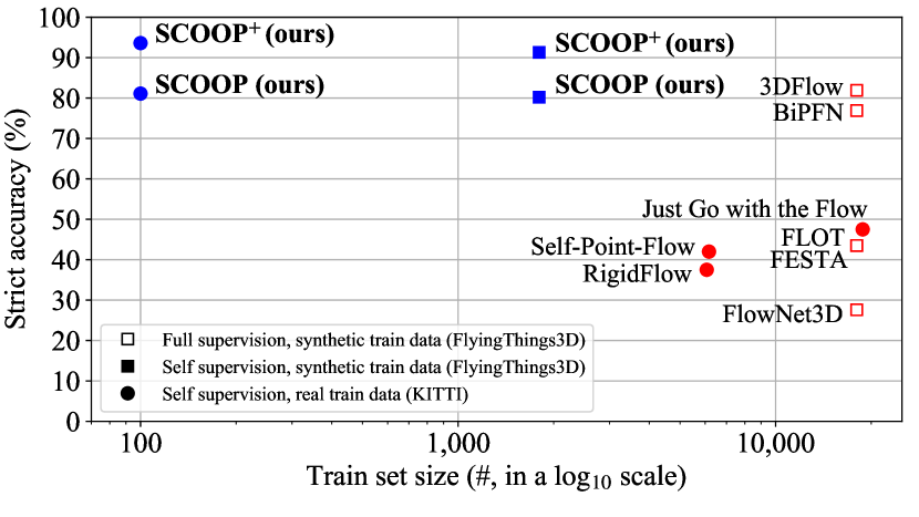
Figure 1: Flow accuracy on the KITTI benchmark vs. the train set size. Our method is trained on one or two orders of magnitude less data while surpassing the performance of the competing techniques [20, 25, 29, 37, 17, 18, 36, 4] by a large margin. Please see Table 1 for the complete details of the evaluation settings.

Liu et al. [20] were among the first to pursue this research avenue. They proposed FlowNet3D, a fully-supervised neural network that learned to regress the flow between 3D point clouds and showed remarkable performance improvement over image-based techniques [1, 35, 23]. Since their method required ground-truth flow annotations, which are scarce for real-world data, they turned to training on a large synthetic dataset that compromised the generalization capability to real-world LiDAR data.

Follow-up works devised self-supervised learning schemes [25, 17] and narrowed the domain gap by training on unannotated LiDAR point cloud pairs. However, similar to Liu et al. [20], they used a regression approach in which the model should learn to compute the flow in the free 3D space. This task is extremely challenging, given the irregular nature of point clouds, and requires a large amount of training data for the network to converge.

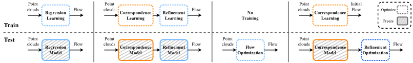
aaaaaaaFlowNet3D [20]	aaaaaaaaaaFLOT [29]	aaaaaaaaaaaNeural Prior [19]	aSCOOP (ours)

Figure 2: Comparison of scene flow approaches. Given a pair of point clouds, FlowNet3D [20] learns to regress the flow in the free 3D space, and the trained model is frozen for testing. FLOT [29] concurrently trains two network components: one that computes point correspondence and another that regresses a correction to the resulting correspondence flow. Neural Prior [19] optimizes the flow between the point clouds from scratch without learning. In contrast to previous work, we take a hybrid approach. We train a pure correspondence model without flow regression, which serves for flow initialization. Then, we directly optimize only the flow refinement at the test-time.

In another line of work [29, 13, 8], researchers leveraged point cloud correspondence for scene flow prediction. In this approach, the flow is computed as the translation of a point in the first point cloud (source) to its softly corresponding point in the second one (target). The softly corresponding point is a weighted sum of target points based on point similarity in a learned latent space. Thus, rather than the challenging regression problem in the 3D ambient space, the flow estimation task boils down to point feature learning and is reduced to the convex combination space [31] of existing target points. However, to relax this constraint, another network component is trained to regress flow corrections. The joint training of point representation and flow refinement burdens the learning process and retains the reliance on large datasets with flow supervision.

Another emerging approach is an optimization-only flow computation [28, 19]. In this case, no training data is involved, and the flow is optimized at run-time for each scene separately. Despite the high accuracy such a dedicated optimization achieves, it requires a long processing time.

We present SCOOP, a hybrid flow estimation method that can be learned from a small amount of training data. SCOOP consists of two parts: a self-supervised neural network for point cloud correspondence and a direct flow refinement optimization module. During the training phase, the network learns to extract point features for soft point matches, which initialize the flow between the point clouds. In contrast to previous work, our network is focused on learning just the point embeddings, allowing its training on a very small dataset, as shown in Figure 1. Additionally, we consider the confidence of the network in the computed correspondences to guide the learning process better.

Then, instead of training another network for regressing flow updates, we define an optimization problem and directly optimize residual flow refinement vectors at run-time. The optimization objective encourages a coherent flow field while retaining the translated source points close to the target point cloud. Our design choices improve the accuracy compared to learning-based methods and reduce the processing time with respect to the optimization-only approach [28, 19]. For both correspondence learning and refinement optimization, we use a self-supervised distance objective and a smoothness prior instead of ground-truth flow labels. Figure 2 presents the difference between our approach and leading previous ones.

In summary, we propose a hybrid flow prediction approach for point clouds based on self-supervised correspondence learning and direct run-time residual flow optimization. Using well-established datasets in the scene flow literature, we show that our approach yields clear performance improvement over existing state-of-the-art methods while using a fraction of the training data and without employing any ground-truth flow supervision.

2 Related Work

Flow regression.  A common approach for scene flow estimation on point clouds is to train a flow regression model [20, 11, 41, 37, 4]. It is a neural network that computes the flow vectors between the point clouds in the ambient 3D space. Liu et al. [20] proposed FlowNet3D, which encoded the point clouds into a latent space, mixed point features with a flow embedding layer, and regressed the scene flow by decoding the mixed point features. FlowNet3D was trained in a fully-supervised manner, using an $l_{2}$ loss with respect to ground-truth flow annotations.

Liu et al. [20] inspired a line of follow-up works [25, 37, 17, 36, 4]. Wang et al. [37] added spatial and temporal attention layers to FlowNet3D’s architecture. In Bi-PointFlowNet [4], the authors propagated features from each point cloud bidirectionally, augmenting the point feature representation. Mittal et al. [25] discarded flow supervision by utilizing a self-supervised nearest neighbor loss and cycle consistency between the forward and reveres scene flows, and Li et al. [17, 18] extracted flow labels for training from the data itself. Similar to the latter methods, we also refrain from ground-truth flow supervision in our training scheme. However, rather than flow regression, we base our technique on soft point matches in the scene, which simplifies the flow estimation problem.

Point cloud correspondence.  Finding correspondences is widely applied to various vision tasks [14, 29, 42, 44]. Several methods have been proposed for dense mapping between non-rigid point cloud shapes [9, 7, 43, 14]. Recently, Lang et al. [14] suggested constructing one point cloud by the other using latent space similarity and the point coordinates themselves rather than regressing the corresponding point cloud [9, 43]. Inspired by Lang’s work, we do not use flow regression in our model and concentrate the learning process on point feature representation. However, while Lang et al. operated on complete shapes with one-to-one correspondence, our method accommodates scenes with partial objects where a perfect match may not exist.

Researchers have taken the correspondence approach to the scene flow problem as well [29, 13, 8]. FLOT [29] computed an optimal transport plan that served for an initial flow between the point clouds and further regressed flow refinement with a series of learned convolutions. Our work builds on FLOT but differs from it in three main aspects. First, we exclude flow regression from our training scheme and instead apply direct run-time optimization to refine the initial correspondence-based flow. Second, we use the model’s confidence in the computed point matches to improve the point feature learning. Third, we do not use any ground-truth flow annotations, neither for the correspondence training nor for the refinement optimization, whereas FLOT relies on fully-supervised scene flow data.

Optimization-based scene flow.  Pontes et al. [28] suggested a scene flow estimation technique that does not involve learning. Instead, the flow was optimized completely at run-time, such that the warped source is close to the target point cloud while demanding the flow to be “as-rigid-as-possible”. Pontes et al. encoded this prior by minimizing the graph Laplacian defined over the source points. In follow-up work [19], the explicit graph was replaced by a neural prior, which implicitly regularized the optimized flow field. In contrast to these papers, we initialize the flow with a learned correspondence model and optimize only the residual flow refinement at run-time.

3 Method

A point cloud is a set of unordered 3D points $X\in\mathbb{R}^{n\times 3}$, where $n$ is the number of points. Given a pair of point clouds of a scene, denoted as $X,Y\in\mathbb{R}^{n\times 3}$ and referred to as source and target, respectively, our goal is to estimate a flow field $F^{*}\in\mathbb{R}^{n\times 3}$ describing the per-point motion from $X$ to $Y$.

We tackle this problem via self-supervised soft correspondence learning between the two point clouds and a direct flow refinement optimization. An overview of the method is shown in Figure 3. First, a deep neural network is used to extract point features. Then, we calculate a matching cost between points in the learned feature space. Based on this cost, we solve an optimal transport problem to compute a softly matched target point for each source point, where the difference between the two is regarded as the correspondence-based flow. Finally, we refine the flow field by demanding its consistency across neighboring source points and obtain our estimated scene flow. In both correspondence learning and flow refinement, no ground-truth flow labels are employed.

3.1 Matching Cost

The cost of matching a point $x_{i}\in X$ to a point $y_{j}\in Y$ is determined based on the point representation learned by a deep neural network. The network consumes the raw point clouds $X$, $Y$ and computes point features $\Phi_{X},\Phi_{Y}\in\mathbb{R}^{n\times d}$, where $d$ is the per-point feature dimension. The network’s architecture is based on PointNet++ [30]. Its details are given in the supplemental material.

Inspired by previous work [29, 17, 14], we first compute the cosine similarity in the learned feature space:

$$S_{ij}=\frac{\Phi_{X}^{i}\cdot(\Phi_{Y}^{j})^{\top}}{||\Phi_{X}^{i}||_{2}||\Phi_{Y}^{j}||_{2}},$$ (1)

where $\Phi_{X}^{i},\Phi_{Y}^{j}\in\mathbb{R}^{d}$ are the $i$’th and $j$’th rows of $\Phi_{X}$ and $\Phi_{Y}$, respectively. Then, the cost is set to

$$C_{ij}=1-S_{ij}$$ (2)

for points with a Euclidean distance less than 10 meters and to $\infty$ otherwise to avoid flow between points too far apart.

3.2 Soft Correspondence

Finding correspondence between the source and target point clouds can be modeled as an optimal transport problem, where each source point is assigned with a mass $\frac{1}{n}$ that is transported to the target points [29, 17]. Similar to FLOT [29], we use the relaxed transport problem:

$$\begin{split}T^{*}=&\operatorname*{\arg\!\min}_{T\in\mathbb{R}_{+}^{n\times n}}\sum_{ij}(C_{ij}T_{ij}+\epsilon T_{ij}(\log T_{ij}-1))\\ &+\lambda(\mathsf{KL}(T1_{n},\frac{1}{n}1_{n})+\mathsf{KL}(T^{\top}1_{n},\frac{1}{n}1_{n})),\end{split}$$ (3)

where $C_{ij}\geq 0$ is the matching cost from Equation 2 and $T_{ij}\geq 0$ is the amount of mass transported between points. The parameters $\epsilon,\lambda\geq 0$ control the relaxation of the problem. $1_{n}\in\mathbb{R}^{n}$ is a vector with all entries equal 1. $\mathsf{KL}$ is the Kullback-Leibler divergence used for soft preservation of the transported mass between the point clouds.

The second term in the summation operation in Equation 3 is an entropic regularization, which enables solving the problem efficiently by the Sinkhorn algorithm [6, 5]. We use this algorithm to estimate the optimal transport matrix $T^{*}$ from $C$ to represent the soft correspondence between the point clouds. The complete derivation of the transport problem and the Sinkhorn algorithm’s details are given in the supplementary material.

3.3 Correspondence-Based Flow

We leverage the optimal transport plan $T^{*}$ to compute correspondence weights for the source and target points for an initial estimate of the scene flow. Different from FLOT [29], which includes all the target points as candidates for each source point, we consider only target points with maximal transport amount from the source point. This design choice focuses our flow estimation pipeline on the most relevant target candidates and improves the method’s results.

For a point $x_{i}\in X$, the matching weights are calculated as follows:

$$w_{ij}=\frac{e^{T^{*}_{ij}}}{\sum_{l\in\mathcal{N}_{Y}(x_{i})}e^{T^{*}_{il}}},$$ (4)

where $\mathcal{N}_{Y}(x_{i})$ is a neighborhood containing the $k_{s}$ indices of the $\{y_{j}\}$ points with the top mass transport $\{T^{*}_{ij}\}$. The softly corresponding point $\hat{y}_{x_{i}}$ to $x_{i}$ is:

$$\hat{y}_{x_{i}}=\sum_{j\in\mathcal{N}_{Y}(x_{i})}{w_{ij}y_{j}},$$ (5)

and the initial estimated flow for the point $x_{i}$ is:

$$f_{i}=\hat{y}_{x_{i}}-x_{i}.$$ (6)

Note that if we define $\widehat{T}^{*}_{ij}=w_{ij}$ for $j\in\mathcal{N}_{Y}(x_{i})$ and $0$ otherwise, we get the initial flow field as:

$$F=\widehat{T}^{*}Y-X=\widehat{Y}-X,$$ (7)

where $\widehat{Y}\in\mathbb{R}^{n\times 3}$ contains the points $\{\hat{y}_{x_{i}}\}$.

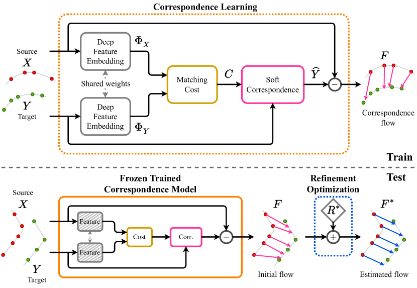
Figure 3: The proposed method. SCOOP includes two components: a learned point cloud correspondence model and a flow refinement module. The model learns deep point embeddings $\Phi_{X},\Phi_{Y}$ to establish soft point matches based on a matching cost $C$ in the latent space. The initial flow $F$ from the training phase is the difference between the softly corresponding point cloud $\widehat{Y}$ and the source point cloud $X$. At the test-time, we freeze the trained model and optimize a residual flow refinement $R^{*}$ to produce a smooth and consistent scene flow $F^{*}$ between the point clouds.

3.4 Training Objective

To learn point representation suitable for scene flow without ground-truth supervision, we apply the flowing loss terms. First, for a tractable flow estimation, we would like each softly corresponding point $\hat{y}_{x_{i}}$ to have a nearby target point $y_{j}$. It may be achieved by the nearest-neighbor distance term, as done by Mittal et al. [25]:

$$\mathcal{D}=\frac{1}{|X|}\sum_{x_{i}\in X}{\min_{y_{j}\in Y}||\hat{y}_{x_{i}}-y_{j}||_{2}^{2}}.$$ (8)

However, the correspondence quality for the source points can vary. For example, points on a flat region will have less distinctive correspondences than points with geometrically unique features. Thus, we augment the distance term in Equation 8 with the matching confidence of each point.

The confidence measure is based on the correspondence similarity that we define as:

$$s_{x_{i}}=\sum_{j\in\mathcal{N}_{Y}(x_{i})}{w_{ij}S_{ij}}.$$ (9)

The value of $s_{x_{i}}$ is in the range $[-1,1]$. To get a confidence value between $0$ and $1$, we trim the negative values, set the matching confidence of $x_{i}$ to be $p_{x_{i}}=\max(s_{x_{i}},0)$, and use $p_{x_{i}}$ to define our confidence-aware distance loss:

$$\mathcal{L}_{dist}=\frac{1}{|X|}\sum_{x_{i}\in X}p_{x_{i}}{\min_{y_{j}\in Y}||\hat{y}_{x_{i}}-y_{j}||_{2}^{2}}.$$ (10)

The loss term $\mathcal{L}_{dist}$ can be minimized by either minimizing $p_{x_{i}}$ or the distance between $\hat{y}_{x_{i}}$ and its nearest neighbor $y_{j}\in Y$. To avoid the degenerate solution of $p_{x_{i}}=0$ for all $x_{i}\in X$, we add a confidence loss term:

$$\mathcal{L}_{conf}=\frac{1}{|X|}\sum_{x_{i}\in X}1-p_{x_{i}},$$ (11)

which penalizes the degenerate solution.

Additionally, to preserve the geometric structure of the source point cloud, we would like the flow field to be smooth. That is, neighboring source points should have a similar flow prediction. Thus, we regularize the learning process with a flow smoothness loss [13]:

$$\mathcal{L}_{flow}=\frac{1}{|X|k_{f}}\sum_{x_{i}\in X}\sum_{l\in N_{X}(x_{i})}{||f_{i}-f_{l}||_{1}},$$ (12)

where $N_{X}(x_{i})$ is the Euclidean neighborhood of $x_{i}$ in $X\setminus x_{i}$ of size $k_{f}$. The overall training objective is:

$$\mathcal{L}_{total}=\mathcal{L}_{dist}+\alpha_{conf}\mathcal{L}_{conf}+\alpha_{flow}\mathcal{L}_{flow},$$ (13)

where $\alpha_{conf}$ and $\alpha_{flow}$ are hyperparameters, balancing the contribution of the different loss terms.

3.5 Flow Refinement Optimization

The advantage of the correspondence-based flow, presented in Equation 7, is that the softly matching points are in the vicinity of the surface of objects in the target scene. However, it limits the flow to the convex hull [31] of points in the target point cloud. We enable the flow to deviate from this constraint by a flow refinement optimization step at run-time.

Instead of training an additional neural network part to regress flow corrections, as done by Puy et al. [29], we directly optimize a flow refinement component $R^{*}\in\mathbb{R}^{n\times 3}$ using the self-supervised distance and smoothness losses defined in Equations 10 and 12, respectively. An illustration of these losses is depicted in Figure 4.

The optimization problem for the flow refinement takes the form:

$$\begin{split}R^{*}=\operatorname*{\arg\!\min}_{R\in\mathbb{R}^{n\times 3}}\frac{1}{|X|}&\sum_{x_{i}\in X}{\min_{y_{j}\in Y}p_{x_{i}}||x_{i}+(f_{i}+r_{i})-y_{j}||_{2}^{2}}\\ +\lambda_{flow}\frac{1}{|X|k_{f}}&\sum_{x_{i}\in X}\sum_{l\in N_{X}(x_{i})}{||(f_{i}+r_{i})-(f_{l}+r_{l})||_{1}},\end{split}$$ (14)

where $r_{i}\in R$ is the flow refinement for point $x_{i}$, and the refined scene flow is $F^{*}=F+R^{*}$. Our flow refinement module further preserves the structure of the source point cloud, where the target points $\{y_{j}\}$ are used as anchors to guide the refined flow and keep the proximity to the underlying target surface.

4 Experiments

Method	Supervision	Train data	Test dataa	$\>EPE\!\downarrow$	$\>AS\!\uparrow$	$\>AR\!\uparrow$	$\>Out.\!\downarrow$
FlowNet3D [20]	Full	FT3Do (18,000)	KITTIo	0.173	27.6	60.9	64.9
FLOT [29]	Full	FT3Do (18,000)	KITTIo	0.107	45.1	74.0	46.3
FESTA [37]	Full	FT3Do (18,000)	KITTIo	0.094	44.9	83.4	-
3DFlow [36]	Full	FT3Do (18,000)	KITTIo	0.073	81.9	89.0	26.1
BiPFN [4]	Full	FT3Do (18,000)	KITTIo	0.065	76.9	90.6	26.4
SCOOP (ours)	Self	FT3Do (1,800)	KITTIo	0.063	79.7	91.0	24.4
SCOOP+ (ours)	Self	FT3Do (1,800)	KITTIo	0.047	91.3	95.0	18.6
JGF [25]	Full + Self + Self	FT3Do (18,000) + nuScenes (700) + KITTIv (100)	KITTIt	0.105	46.5	79.4	-
SPF [17]	Self + Self	KITTIr (6,068) + KITTIv (100)	KITTIt	0.089	41.7	75.0	-
RigidFlow [18]	Self	KITTIr (6,068)	KITTIt	0.117	38.8	69.7	-
SCOOP (ours)	Self	KITTIv (100)	KITTIt	0.052	80.6	92.9	19.7
Graph Prior [28]	Self	N/A (optimization-only)	KITTIt	0.082	84.0	88.5	-
Neural Prior [19]	Self	N/A (optimization-only)	KITTIt	0.036	92.3	96.2	-
SCOOP+ (ours)	Self	KITTIv (100)	KITTIt	0.039	93.6	96.5	15.2

Table 1: Quantitative comparison. We compare scene flow evaluation metrics for different supervision settings, train data, and test data. The number of training examples is indicated in parentheses. $EPE$, $AS$, $AR$, and $Out.$ stand for End-Point-Error, Strict Accuracy, Relaxed Accuracy, and Outliers, respectively. The symbol ⁺ indicates an evaluation using all the points in the test point clouds, as done for the optimization-only methods [28, 19]. While other baselines apply fully-supervised training, our method yields better performance without employing ground-truth flow labels. Besides, SCOOP can be trained only on KITTI_v, with as few as 100 training instances. In contrast, alternative learning-based methods use additional training data, such as nuScenes, or a large dataset, such as KITTI_r. Please see further details in subsections 4.1 and 4.2.

In this section, we evaluate SCOOP’s performance using widely spread datasets and compare it with recent state-of-the-art (SOTA) works on scene flow estimation. Additionally, we demonstrate the influence of the flow refinement module, analyze the performance and run-time duration, and verify our design choices with an ablation study.

4.1 Experimental Setup

Datasets.  We adopt two common datasets in the scene flow literature, FlyingThings3D [22] and KITTI [23, 24]. Originally, these benchmarks did not include point cloud data. They were processed to a point cloud format by Liu et al. [20] and denoted as FT3D_o and KITTI_o, respectively.

FT3D_o is a large-scale synthetic dataset with 18,000/2,000 train/validation scene examples of randomly moving objects from the ShapeNet collection [3]. Each example contains a pair of point clouds and ground-truth flow vectors. Since the objects’ motion is randomized, they may appear or disappear from the view of the scene and create occlusions. The dataset also includes a mask for points whose flow is invalid due to occlusions.

The KITTI_o dataset contains 150 real-world LiDAR scenes. Every scene includes source and target point clouds with flow annotations for the source points. Ground points are removed, and the source points are considered to have a valid flow [20]. KITTI_o was further split by Mittal et al. [25] into sets of 100 and 50 examples, marked as KITTI_v and KITTI_t, respectively, for fine-tuning experiments. Li et al. [17] also built a large unlabeled LiDAR dataset for self-supervised learning on real-world data. They took raw LiDAR scans from the KITTI scenes [23, 24], disjoint from the KITTI_o data, and created a training set of 6,068 instances denoted as KITTI_r.

Figure 4: Illustration of the flow refinement objective. The initial flow $\{f_{i}\}$ stems from the translation of the source points $\{x_{i}\}$ (red) to their softly corresponding ones $\{\hat{y}_{x_{i}}\}$ (magenta). The flow is refined with a distance loss that keeps the proximity of the translated points to the target points $\{y_{j}\}$ (green) and a smoothness loss that encourages similar flow vectors (dashed purple) for neighboring points. The optimization process results in a flow field $\{f_{i}^{*}\}$ (blue) that preserves the structure of the source point cloud and warps it close to the implicit surface of the target point cloud.

Evaluation metrics.  We use well-established evaluation metrics from previous works [20, 25, 29]: End-Point-Error $EPE\>[m]$, Strict Accuracy $AS\>[\%]$, Relaxed Accuracy $AR\>[\%]$, and Outliers $Out.\>[\%]$. These metrics are based on the point error $e_{i}$ and the relative error $e_{i}^{rel}$:

$$e_{i}=||f_{i}^{*}-f_{i}^{gt}||_{2},\quad e_{i}^{rel}=\frac{||f_{i}^{*}-f_{i}^{gt}||_{2}}{||f_{i}^{gt}||_{2}},$$ (15)

where $f_{i}^{*}$ and $f_{i}^{gt}$ are the predicted and ground-truth flow for point $x_{i}$, respectively. The $EPE$ is the average point error, measured in meters; $AS$ is the percentage of points whose $e_{i}<0.05\>[m]$ or $e_{i}^{rel}<5\%$; $AR$ is the percentage of points for which $e_{i}<0.1\>[m]$ or $e_{i}^{rel}<10\%$; and $Out.$ is the percentage of points with $e_{i}>0.3\>[m]$ or $e_{i}^{rel}>10\%$.

Implementation details.  SCOOP is implemented in PyTorch [27], where the publicly available PointNet++ [30] implementation is adapted for our point feature embedding. The model is trained on $n=2,\!048$ points, sampled at random from the source and target point clouds of the scene examples. Only the 3D coordinates of the points are used as input to the model. The parameters $\epsilon$ and $\lambda$ from Equation 3 are defined as learnable variables and optimized as part of the learning process. The point feature dimension is $d=128$. For the neighborhood sizes we use $k_{s}=64$, $k_{f}=32$, and the losses’ hyperparameters are set to $\alpha_{conf}=0.1$, $\alpha_{flow}=10$.

As in previous work [20, 29, 25, 18], we evaluate SCOOP on point clouds of 2,048 points randomly sampled from the source and target. However, the full point clouds of KITTI_o and KITTI_t are an order of magnitude larger and have different cardinality. Thus, for a complete evaluation of the entire scene flow, we also utilize our method (denoted as SCOOP⁺ for this case) to exploit the whole point cloud information and test the performance for the original resolution. Additional implementation details appear in the supplementary.

Baseline methods.  Our method is contrasted with the recent methods FlowNet3D [20], FLOT [29], FESTA [37], 3DFlow [36], and BiPFN [4]. These methods require ground-truth flow supervision. Additionally, we compare our results with the recent self-supervised flow models of Mittal et al. [25] and Li et al. [17, 18], and the optimization-based techniques Graph Prior [28] and Neural Prior [19].

4.2 Scene Flow Results

Cross-dataset evaluation.  We demonstrate the generalization power of SCOOP by training it on the FT3D_o and testing its performance on KITTI_o. Table 1 summarises the results. The alternative methods [20, 29, 37, 36, 4] are trained on FT3D_o in a fully-supervised fashion: their models are learned with the ground-truth flow information, and the points with an occluded flow are excluded from the training objective using the mask provided in the dataset.

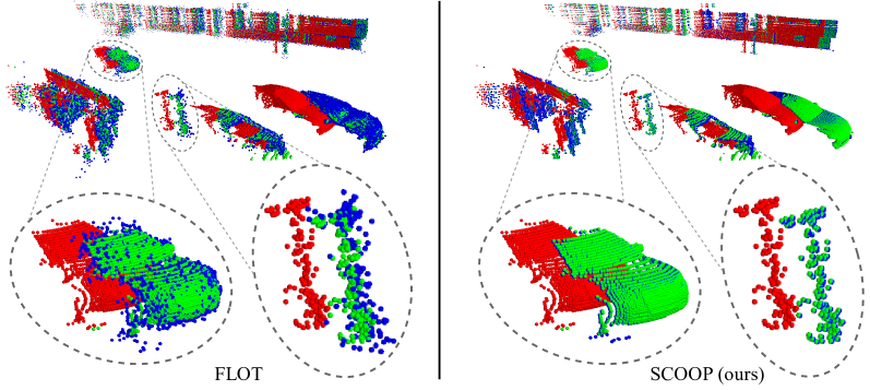
Figure 5: Visual comparison of scene flow results for a KITTI_o example scene. The training was done on the FT3D_o dataset. The source and target point clouds are shown in red and green, respectively. The warped source point cloud by FLOT [29] (left) and by our method (right) is presented in blue. While the result of FLOT deviates from the surface of the target, SCOOP preserves the source point cloud’s structure and computes its accurate flow.

In contrast, our model is trained in a completely self-supervised manner. We assume no knowledge of the flow annotations nor the occlusion mask and do not use them in our losses. Additionally, we use only 1,800 randomly selected examples from FT3D_o, while the competitors employ all 18,000 scene instances. Still, SCOOP improves over the SOTA method BiPFN [4] in all the evaluation metrics. Moreover, utilizing the entire point cloud data further increases our performance.

FlowNet3D [20], FESTA [37], 3DFlow [36], and BiPFN [4] are regression-based networks that predict the flow in the 3D ambient space. The models adapt to the characteristics of the synthetic training set, and the generalization to the real-world test data is limited. FLOT [29] leverages point cloud correspondence based on learned point features, which eases the flow prediction problem. However, it also jointly learns to regress a flow correction component that burdens the point representation training process.

SCOOP, on the other hand, is focused only on learning point embeddings suitable for scene flow estimation, guided by our self-supervised losses. It extracts discriminative features, which transfer well across the FT3D_o and KITTI_o datasets, and enables to compute the correspondence-based flow between the point clouds. In contrast to FLOT, we delegate the flow refinement process to the test phase, directly optimize it in a self-supervised fashion, and surpass their flow estimation performance.

Figure 5 shows a visual comparison between the results of FLOT and our method. The warped source point cloud by FLOT is noisy, and the structure of objects in the scene is compromised. On the contrary, SCOOP produces a coherent flow field across neighboring points, preserves their local geometry, and accurately predicts the scene flow. Additional visualizations are presented in the supplementary.

Training on a small dataset.  Since our model does not include a flow regression component and has to learn only point features, it can be trained on a very limited amount of data. To demonstrate this ability, we train it from scratch on the 100 point cloud pairs of KITTI_v and use KITTI_t for testing. The results of this experiment are presented in Table 1.

Different from our work, the competing methods of Mittal et al. [25] and Li et al. [17, 18] are based on flow regression and require a large amount of training data. Mittal et al. utilize a fully-supervised pre-training on FT3D_o, and the additional outdoor flow dataset nuScenes [2], before fine-tuning on KITTI_v. Li et al. [17, 18] train their model on the large KITTI_r dataset. Our SCOOP outperforms these other methods while being trained only on KITTI_v, which is almost two orders of magnitudes smaller than KITTI_r.

The pure optimization methods [28, 19] find the solution per scene separately, which might lead to sub-optimal local minima. In contrast, we leverage the correspondence statistics learned from the data and adapt the initial flow to the scene at hand by our residual run-time optimization. The initial correspondence flow serves as a good starting point for the optimization phase, yielding a similar or better final result compared to the optimization-only alternatives.

The influence of flow refinement.  Our flow results before and after refinement are presented in Figure 6. Posing the learning part of SCOOP as a correspondence problem enables its effective training on a small dataset. However, the flow predictions from the training phase are confined to a linear combination of existing target points, which may not represent the exact flow of the scene. Moreover, wrong matches for the source points can occur and cause flow errors. In such cases, our refinement module comes into play.

Given the output flow from the trained correspondence model, the refinement module optimizes correction vectors subject to two objectives: a warped source point should be close to a target point; neighboring source points should have a similar flow. These objectives help fixing inconsistencies in the flow field and increase the flow accuracy. As seen in Figure 6, our refinement step improves the initial flow estimation and results in an accurate flow field, which is similar to the ground-truth scene flow.

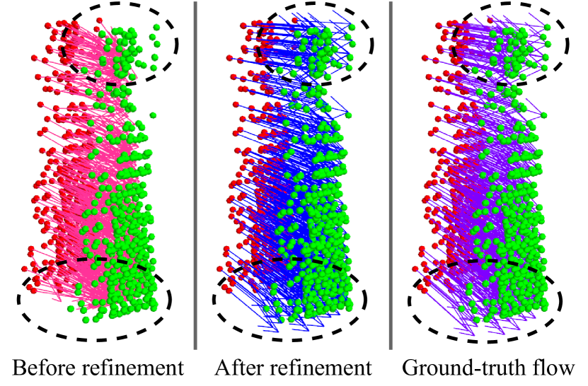
Figure 6: The flow refinement effect. We demonstrate the effect on data from KITTI_t. The source point cloud is in red, and the target is in green. Our correspondence model was trained on the KITTI_v dataset, and its flow estimation before refinement is shown in magenta (left). The optimized refined flow is presented in blue (center). We also show the ground-truth scene flow in purple for reference (right). The refined flow better covers the target point cloud (top center ellipse). It also breaches the convex hull of the given target points and enables computing the correct flow for source points whose target is missing (bottom center ellipse).

4.3 Performance and Time Analysis

We analyze the performance-time trade-off in Figure 7 by recording the $EPE$ and inference time for different methods. The measurements were done on an Nvidia Titan Xp GPU for computing the flow for complete point clouds of the KITTI_t dataset.

Network-only methods [25, 17, 18] tend to be fast but with limited accuracy. Optimizing the flow prediction separately for each scene [19] results in a low $EPE$. However, it takes a long time. Our hybrid method bridges the trade-off gap between these two approaches. SCOOP⁺ offers a working point with more than 50% error reduction over the feed-forward models and about $8\times$ faster inference time than the optimization-only Neural Prior work. SCOOP⁺ also enables a different balance between time and performance, as seen in Figure 7. By reducing the number of run-time optimization steps, the user can shorten the inference time, achieving a working point closer to that of the network-only models.

4.4 Ablation Study

The design choices in our method are verified by ablation experiments presented in Table 2. We change one element each time and keep all the others the same. The following ablative settings were examined: (a) use all target points for soft correspondence instead of the ones with the highest transport amount (Equation 5); (b) ignore the point matching confidence by setting $p_{x_{i}}=1$ in Equation 10 and $\alpha_{conf}=0$ in Equation 13; (c) exclude the smoothness flow loss $\mathcal{L}_{flow}$ from Equation 13; and (d) turn off the flow refinement module.

The ablation study validates the contribution of the proposed components to the method’s performance. Considering a subset of target points for correspondence enables the model to concentrate on the most relevant candidates for flow estimation. The matching confidence emphasizes the influence of the more confident points in our confidence-aware distance loss $\mathcal{L}_{dist}$. The smoothness loss term is important for regularizing the point representation learning to obtain similar features across neighboring points. Lastly, our flow refinement optimization improves the consistency of the flow field and reduces the $EPE$ substantially. In the supplementary material, we provide an ablation study on the FT3D_o train set size and find that a 10% fraction of the data suffices for our method to realize its potential.

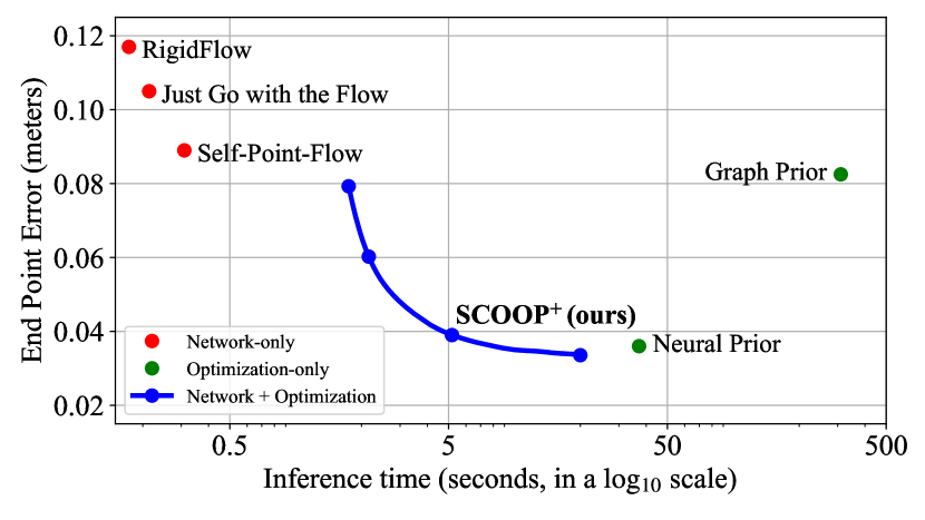
Figure 7: Flow estimation error vs. inference time for the KITTI_t dataset. SCOOP⁺ has a lower error than the network-only models and a shorter inference time than the optimization-only methods. It also allows different balances along the error and time trade-off, as presented by the blue curve.

Setting	$EPE\!\downarrow$	$AS\!\uparrow$
(a) All target points as candidates ($k_{s}=n$)	0.047	91.1
(b) W/O confidence ($p_{x_{i}}=1$, $\alpha_{conf}=0$)	0.044	90.3
(c) W/O smoothness loss term ($\alpha_{flow}=0$)	0.056	86.6
(d) W/O flow refinement ($R^{*}=0$)	0.115	43.8
Our complete method	0.039	93.6

Table 2: Component ablative settings. SCOOP was trained on KITTI_v and evaluated on KITTI_t. The results show that the best performance is obtained with our complete method. Additional details about the ablation experiments are given in subsection 4.4.

5 Conclusions

This paper presented SCOOP, a novel self-supervised scene flow estimation method for 3D point clouds based on correspondence learning and flow refinement optimization. Previous works suggested learning a flow regression model, training a neural network that jointly learned point cloud correspondence and flow refinement, or optimizing the flow completely at run-time without learning.

In contrast, we split the flow prediction process into two simpler problems. Our correspondence model is focused only on learning point features to initialize the flow from soft matches between the point clouds. Then, we directly optimize a residual flow refinement at run-time. This approach enables SCOOP to be trained on a small set of point cloud scenes without utilizing ground-truth supervision while outperforming state-of-the-art fully-supervised and self-supervised learning methods, as well as optimization-based alternative techniques.

Supplementary Material

We provide more information regarding our flow estimation method SCOOP. Section A presents the derivation of point cloud correspondence as an optimal transport problem and the solution by the Sinkhorn algorithm. Section B includes additional results for the experiments presented in the paper. In Section C, we report the results of an additional experiment on a non-occluded data version. Finally, section D elaborates on our implementation details, including network architecture, training and inference procedure, and the optimization settings of SCOOP.

Appendix A Correspondence as Optimal Transport

As mentioned in the paper, our correspondence-based flow between the point clouds $X,Y\in\mathbb{R}^{n\times 3}$ builds on the optimal transport formulation presented in FLOT [29]. For completeness, we briefly review the optimal transport problem and the Sinkhorn algorithm for solving it.

We begin with a hypothetical perfect case, where each source point $x_{i}\in X$ has an exact matching target point $y_{j}\in Y$. Thus, the flow field holds:

$$X+F^{*}=\Pi Y,$$ (16)

where $\Pi\in\{0,1\}^{n\times n}$ is a permutation matrix representing the correspondence between the point clouds, with $\Pi_{ij}=1$ if $x_{i}$ matches $y_{j}$ and $\Pi_{ij}=0$ otherwise.

In this case, estimating the point correspondences can be modeled as an optimal transport problem [29]. Assuming that each point in $X$ has a mass $\frac{1}{n}$ and each point in $Y$ receives a mass $\frac{1}{n}$, the optimal mass transport is given by:

$$\begin{split}T^{*}=&\operatorname*{\arg\!\min}_{T\in\mathbb{R}_{+}^{n\times n}}\sum_{ij}C_{ij}T_{ij}\\ &\text{such that}\quad T1_{n}=\frac{1}{n}1_{n},\quad T^{\top}1_{n}=\frac{1}{n}1_{n},\end{split}$$ (17)

where $1_{n}\in\mathbb{R}^{n}$ is a vector with all entries equal 1, $C_{ij}\geq 0$ is the transport cost from point $x_{i}$ to point $y_{j}$, and $T_{ij}\geq 0$ is the amount of mass transported between these points. The two terms on the second row of Equation 17 are mass constraints, demanding that the total mass delivered from each source point and received by each target point is exactly $\frac{1}{n}$. $T^{*}$ is optimal in the sense that the mass is transported from $X$ to $Y$ with minimal cost.

In practice, usually, there is no perfect match between the point clouds due to objects appearing in or disappearing from the scene or different points sampled on the scene’s surface, and the mass constraints in Equation 17 do not hold. Thus, instead of Equation 17, we used the relaxed version of the transport problem presented in Equation 3 in the paper. The relaxed transport problem is solved by the Sinkhorn algorithm [6, 5], which estimates $T^{*}$ from $C$. We provide the algorithm’s details in Algorithm 1. In our implementation, the number of iterations $M$ is set to 1.

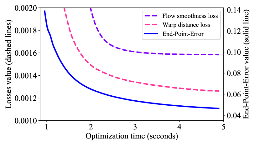
Figure 8: Refinement evolution. SCOOP was trained on FT3D_o and evaluated on KITTI_o. We present the refinement loss values and the corresponding End-Point-Error ($EPE$) during the optimization process. The losses are effectively minimized and result in a substantial reduction of the flow estimation error.

Method	Refinement	$\>EPE\!\downarrow$	$\>AS\!\uparrow$	$\>AR\!\uparrow$	$\>Out.\!\downarrow$
FLOT [29]	✗	0.142	30.6	61.9	57.6
FLOT [29]	✓	0.048	89.0	93.5	20.4
SCOOP+ (ours)	✗	0.139	36.1	63.6	54.9
SCOOP+ (ours)	✓	0.047	91.3	95.0	18.6

Table 3: Our refinement optimization for another method. FLOT and SCOOP were trained on 1,800 examples from FT3D_o and tested on KITTI_o, without or with our flow refinement component. The proposed refinement module considerably improves the flow estimation performance for both methods.

Appendix B Additional Results

B.1 Refinement Evolution

We examine the relationship between our self-supervised losses in the flow refinement process, given in Equation 14, and the resulting End-Point-Error metric ($EPE$), defined in subsection 4.1. Figure 8 shows the results (for better visualization, we multiply the smoothness loss value by a factor of $4\cdot 10^{-2}$). During run-time, we minimize our smoothness and distance losses without using ground-truth flow labels. As a byproduct, the $EPE$ is reduced as well. This experiment implies that our refinement objective in Equation 14 correlates with the flow estimation error and serves as a good proxy for its minimization.

B.2 Refinement Optimization for Another Method

A natural question is whether a flow estimation method other than ours can benefit from the proposed refinement optimization module. To address this question, we trained FLOT [29] on 1,800 examples from the FT3D_o train set, as done for our method. Then, we evaluated FLOT’s performance on the KITTI_o data without or with our run-time refinement (with correspondence confidence equal to 1 for all the source points). Table 3 summarizes the results.

Training on a 10% fraction of FT3D_o data degrades FLOT’s performance in comparison to using the complete dataset, as reported in Table 1 in the main body. However, our refinement optimization substantially contributes to the flow precision of FLOT and even yields better results compared to using the whole training set. This experiment hints that our proposed run-time refinement is not tailor-made for SCOOP and can benefit another method as well.

B.3 Qualitative Results

In Figure 9, we present additional results of SCOOP for KITTI_o data for various challenging cases. For example, our method can gracefully handle different point densities, as cars with varying distances from the LiDAR sensor exhibit. In addition, since we require consistency of the flow field over the point cloud, SCOOP can correctly estimate the flow for an object with a repetitive structure, such as a fence. At the same time, our flow estimation method is versatile. It copes with shapes of different geometry and size, such as the pole and the facade. SCOOP can also predict translation vectors of different directions and magnitudes, as for the car and pole.

Data: $\text{cost matrix}\;C,\>\text{parameters}\;\epsilon,\lambda\geq 0,\>M>0.$

Result: $\text{optimal transport matrix}\;T^{*}.$

$T\leftarrow\exp(-C/\epsilon)$;

$a\leftarrow\frac{1}{n}1_{n}$;

for $m=1,\dots,M$ do

       $b\leftarrow(\frac{1}{n}1_{n}/(T^{\top}\!a))^{\lambda/(\lambda+\epsilon)}$;

       $a\leftarrow(\frac{1}{n}1_{n}/(Tb))^{\lambda/(\lambda+\epsilon)}$;

      

end for

$T^{*}\leftarrow\operatorname{diag}(a)\>T\operatorname{diag}(b)$;

Algorithm 1 The Sinkhorn Algorithm.

B.4 Ablation Runs

In Table 4, we report results of our method for different train set sizes of FT3D_o. The table shows that a 10% fraction of the FT3D_o data is sufficient for SCOOP to converge to its optimal performance.

Table 5 presents additional ablation experiments. In this round, we examined the following settings (one configuration change at a time). (a) Turn off the Sinkhorn normalization. In this case, we used $T=\exp(-C/\epsilon)$ instead of $T^{*}$ from Algorithm 1, and the correspondence construction in Equations 4 and 5 was done with target points with minimal matching cost $C$ rather than maximal transport $T^{*}$. (b) Apply a higher number of iterations in the Sinkhorn algorithm by setting $M=3$ instead of $M=1$. (c) Linear normalization for the correspondence confidence $p_{x_{i}}=(s_{x_{i}}+1)/2$ instead of the non-linear truncation $p_{x_{i}}=\max(s_{x_{i}},0)$. In all these settings, the difference in the method’s performance was small, implying its robustness to such configuration changes.

FT3Do number of training examples	180	1,800	18,000
KITTIo $EPE\!\downarrow$	0.057	0.047	0.047

Table 4: Train set size ablation. We trained SCOOP on the FT3D_o dataset using a different number of instances and measured the $EPE$ on the KITTI_o dataset. A subset of only 1,800 training examples is sufficient for our technique.

Setting	$\>EPE\!\downarrow$	$\>AS\!\uparrow$	$\>AR\!\uparrow$	$\>Out.\!\downarrow$
(a) W/O Sinkhorn	0.042	91.6	95.9	16.1
(b) 3 Sinkhorn iterations	0.040	92.9	96.4	15.3
(c) Linear $p_{x_{i}}$ normalization	0.040	93.5	96.4	15.5
The proposed method	0.039	93.6	96.5	15.2

Table 5: Additional ablations. We trained SCOOP with different configurations on KITTI_v and evaluated its performance on KITTI_t. The table shows that our method is robust to these configuration variations. Details about the ablative settings appear in subsection B.4.

B.5 Limitation

A failure case of SCOOP is presented in Figure 11. When a part of the source scene is completely missing from the target, the correspondence to existing target points is inaccurate, and the flow predicted by our method does not represent the motion of that part. In future work, we plan to detect such wrong matches by remaining inconsistencies in the flow field and leverage the global motion of the scene to deduce the flow for completely occluded regions.

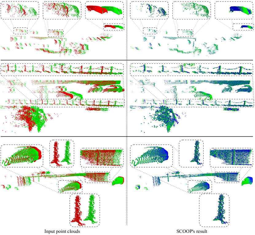
Figure 9: Visual results. We applied SCOOP to different LiDAR scenes. The source and target input point clouds are presented in red and green, respectively, and the warped source is shown in blue. Our method is able to predict the scene flow in a variety of challenging scenarios, such as varied point cloud density (top), repetitive structures (middle), and objects with different sizes and motions (bottom).

Appendix C An Additional Experiment

In addition to FT3D_o and KITTI_o, Gu et al. [11] prepared another point cloud version of the FlyingThings3D and KITTI datasets, denoted as FT3D_s and KITTI_s, respectively. In their version, all occluded points are removed, and each source point has a matched target point. This version of the datasets is also popular in the scene flow literature, and for a comprehensive evaluation, we report our method’s results for this case as well. Additional details about the datasets appear in subsection D.2.

Since the point clouds produced by Gu et al. have no occlusions, we adapt our method to the nature of this data. Instead of the distance loss from Equation 10, we use the bidirectional Chamfer Distance loss [41, 14]:

$$\begin{split}\mathcal{L}_{cd}&=CD(\widehat{Y},Y)=\\ &\frac{1}{|\widehat{Y}|}\sum_{\hat{y}\in\widehat{Y}}{\min_{y\in Y}||\hat{y}-y||_{2}^{2}}+\frac{1}{|Y|}\sum_{y\in Y}{\min_{\hat{y}\in\widehat{Y}}||y-\hat{y}||_{2}^{2}},\end{split}$$ (18)

where $\widehat{Y}$ is the softy corresponding point cloud to the source point cloud $X$ (from Equation 7), and $Y$ is the target point cloud. The Chamfer Distance is also used in the refinement process and replaces the first term in the optimization objective in Equation 14. If we define $\widehat{Y}_{r}=\widehat{Y}+R$, the updated distance loss term for the flow refinement optimization is $CD(\widehat{Y}_{r},Y)$. The rest of our method’s formulation remains the same.

Following the evaluation protocol of previous work [11, 29, 13], we train SCOOP on FT3D_s and evaluate the performance on the test set of FT3D_s and on the KITTI_s data. Different from prior work, we use only 10% of the FT3D_s training data, which suffices for our correspondence model to coverage. The evaluation metrics are the same as those in the main body, detailed in subsection 4.1. For both training and testing, we use point clouds with $n=8192$ points.

Tables 6 and 7 present our test results for FT3D_s and KITTI_s, respectively, compared to abundant recent alternative methods. While trained only on a 10% fraction of the data, SCOOP achieves competitive results compared to other self-supervised methods on FT3D_s. On the KITTI_s dataset, we surpass the performance of both self and fully-supervised methods for all the evaluation metrics. For example, SCOOP improves the $EPE$ metric by 37% over the very recent Bi-PointFlowNet work [4], reducing the flow estimation error from $0.030$ to $0.019$ meters. These results suggest that our method is highly effective for the real-world KITTI_s data.

Method	Sup.	$\>EPE\!\downarrow$	$\>AS\!\uparrow$	$\>AR\!\uparrow$	$\>Out.\!\downarrow$
FlowNet3D [20]	Full	0.114	41.3	77.1	60.2
HPLFlowNet [11]	Full	0.080	61.4	85.6	42.9
PointPWC-Net [41]	Full	0.059	73.8	92.8	34.2
FLOT [29]	Full	0.052	73.2	92.7	35.7
PV-RAFT [40]	Full	0.046	81.7	95.7	29.4
FlowStep3D [13]	Full	0.046	81.6	96.1	21.7
HCRF-Flow [16]	Full	0.049	83.4	95.1	26.1
RCP [10]	Full	0.040	85.7	96.4	19.8
Rigid3DSceneFlow [8]	Full	0.052	74.6	93.6	36.1
3D-OGFlow [26]	Full	0.036	87.9	-	19.7
SCTN [15]	Full	0.038	84.7	96.8	26.8
3DFlow [36]	Full	0.028	92.9	98.2	14.6
Bi-PointFlowNet [4]	Full	0.028	91.8	97.8	14.3
Ego-motion [32]	Self	0.170	25.3	55.0	80.5
PointPWC-Net [41]	Self	0.121	32.4	67.4	68.8
Self-Point-Flow [17]	Self	0.101	42.3	77.5	60.6
FlowStep3D [13]	Self	0.085	53.6	82.6	42.0
RSFNet [12]	Self	0.075	58.9	86.2	47.0
RCP [10]	Self	0.077	58.6	86.0	41.4
RigidFlow [18]	Self	0.069	59.6	87.1	46.4
SCOOP (ours)	Self	0.084	56.7	85.1	48.5

Table 6: Quantitative comparison on the FT3D_s test set. All the methods were trained on the train split of FT3D_s. Our method is on par with other self-supervised methods.

Method	Sup.	$\>EPE\!\downarrow$	$\>AS\!\uparrow$	$\>AR\!\uparrow$	$\>Out.\!\downarrow$
FlowNet3D [20]	Full	0.177	37.4	66.8	52.7
HPLFlowNet [11]	Full	0.117	47.8	77.8	41.0
PointPWC-Net [41]	Full	0.069	72.8	88.8	26.5
FLOT [29]	Full	0.056	75.5	90.8	24.2
PV-RAFT [40]	Full	0.056	82.3	93.7	21.6
FlowStep3D [13]	Full	0.055	80.5	92.5	14.9
HCRF-Flow [16]	Full	0.053	86.3	94.4	18.0
RCP [10]	Full	0.048	84.9	94.5	12.3
Rigid3DSceneFlow [8]	Full	0.042	84.9	95.9	20.8
3D-OGFlow [26]	Full	0.039	88.2	-	17.5
SCTN [15]	Full	0.037	87.3	95.9	17.9
3DFlow [36]	Full	0.031	90.5	95.8	16.1
Bi-PointFlowNet [4]	Full	0.030	92.0	96.0	14.1
Ego-motion [32]	Self	0.415	22.1	37.2	81.0
PointPWC-Net [41]	Self	0.255	23.8	49.6	68.6
Self-Point-Flow [17]	Self	0.112	52.8	79.4	40.9
FlowStep3D [13]	Self	0.102	70.8	83.9	24.6
RSFNet [12]	Self	0.092	74.7	87.0	28.3
RCP [10]	Self	0.076	78.6	89.2	18.5
RigidFlow [18]	Self	0.062	72.4	89.2	26.2
SCOOP (ours)	Self	0.019	97.1	98.5	10.7

Table 7: Quantitative comparison on the KITTI_s data. All the methods were trained on the train split of FT3D_s. SCOOP outperforms all the compared alternatives, both the self-supervised and the fully-supervised ones.

Appendix D Implementation Details

D.1 Network Architecture

The point feature extraction is done by a neural network based on the PointNet++ architecture [30]. The network includes 3 set-convolution layers, which increase the feature channels per point. Each layer contains a multi-layer perceptron, interleaved with instance normalization and a leaky ReLU activation with a negative slope of $-0.1$. After each convolutional layer, the point features are aggregated by a max pooling operation from 32 Euclidean nearest neighbor points. The coordinate difference between the point and its neighbors is concatenated to the input features of every set-convolution layer. Table 8 details the feature dimensions of the network’s layers.

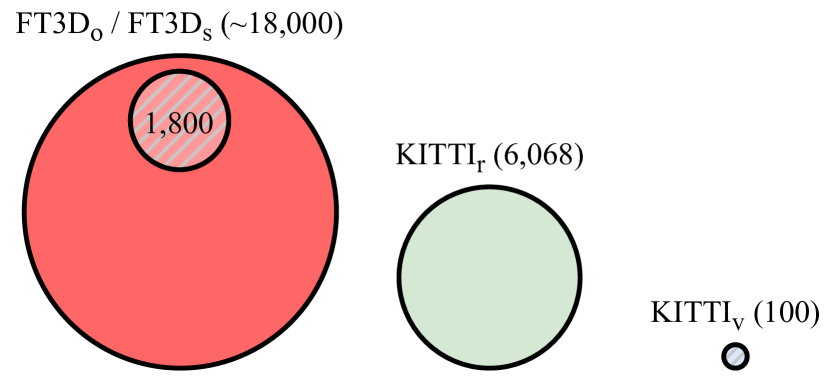
Figure 10: Visual illustration of the training datasets’ size. We use a small amount of data for training (stripe pattern) compared to the amount used by others (solid pattern).

Figure 11: A failure example. We show the source point cloud in red, the target in green (left), the translated source by SCOOP in blue (middle), and the translated source by the ground-truth flow in purple (right). A set of source points whose target is completely occluded is marked with a gray ellipse. Its warp by the estimated and the ground-truth flow is delineated by a blue ellipse and a purple ellipse, respectively. Our method struggles to predict the correct flow in such a case.

D.2 Training and Inference

Training dataset size.  We illustrate the size of the training datasets in Figure 10. As explained in the paper (subsection 4.2), SCOOP is a data-light method that requires much less training data than other learning-based methods.

Occluded data version.  The FT3D_o dataset contains point clouds of 8,192 points, where the z-axis coincides with the depth axis, and the maximal z-value is limited to 35 meters [20]. In the KITTI_o dataset, there are several tens of thousands of points per scene, with a different number of points for the source and target point clouds, denoted as $N_{s}$ and $N_{t}$, respectively. We align the z-axis of KITTI_o to the depth axis and trim the maximal z-value to 35 meters, as done for the FT3D_o data [29].

Network architecture
$concat(\text{coordinates}\>(3),\text{neighbors' coordinate difference}\>(3))$
$SetConv(32,32,32)$
$neighbors\;max\;pooling\>(32)$
$concat(\text{features}\>(32),\text{neighbors' coordinate difference}\>(3))$
$SetConv(64,64,64)$
$neighbors\;max\;pooling\>(64)$
$concat(\text{features}\>(64),\text{neighbors' coordinate difference}\>(3))$
$SetConv(128,128,128)$
$neighbors\;max\;pooling\>(128)$

Table 8: The architecture of the feature extraction model. The values in parentheses indicate the per-point feature dimension at each network stage. $concat$ represents a concatenation operation. The coordinate difference and max pooling operation are computed with a neighborhood of 32 nearest points in the Euclidean space. $SetConv$ is the set convolution described in subsection D.1, where the numbers in its parentheses refer to the filter sizes of the multi-layer perceptron.

For memory-efficient training, SCOOP is trained on point sets with the same number of $n=2,\!048$ points sampled at random from the original point clouds. Following previous work [20, 29, 25, 18], we evaluate SCOOP on small test point clouds of randomly sampled 2,048 points. However, we also employ our method to infer the flow for all the points $N_{s}$ in the source point cloud, as explained next.

At the test-time, we randomly shuffle the source points and the target points, divide them into disjoint chunks of $n=2,\!048$ points, and compute the point features $\Phi_{X}$ and $\Phi_{Y}$ for each chunk, as done in the training stage. If the number of points is not divided by $n$, we pad with randomly selected points from within the point cloud to the closest multiple of $n$. Then, for each source chuck, we calculate the matching cost with respect to all the points in the target, obtain a cost matrix $C_{chunk}\in\mathbb{R}^{n\times N_{t}}$, and compute the correspondence-based flow $F_{chunk}\in\mathbb{R}^{n\times 3}$. Afterward, we collect the flow from the different chunks, remove the padded points (if any), and get the per-point flow $F\in\mathbb{R}^{N_{s}\times 3}$.

Train/Test data (#points)	$k_{f}$	$\lambda_{flow}$	Gradient	Update
			steps	rate
FT3Do/KITTIo (2,048)	32	1.0	1000	0.05
KITTIv/KITTIt (2,048)	32	1.0	1000	0.05
FT3Do/KITTIo (29,951)	32	1.0	150	0.2
KITTIv/KITTIt (30,814)	32	1.0	150	0.2
FT3Ds/FT3Ds (8,192)	16	1.0	1000	0.1
FT3Ds/KITTIs (8,192)	32	1.0	1000	0.05

Table 9: Refinement hyperparameters. The table details the values we used for our flow refinement optimization process for different dataset settings. For each setting, we indicate the train/test datasets and the average number of points in the test point clouds.

Our inference process for the complete point clouds has several advantages. First, it can be used for source and target point clouds with different cardinality since each point cloud is padded to a multiple of $n$. Second, as we extract point features in chunks of $n$ points, the process remains memory-efficient and emulates inputs to the network similar to the training phase. Third, it utilizes the complete point information from the target by computing the cost matrix and correspondence flow at the original target point cloud resolution.

Similarly, we perform the flow refinement optimization at the full source and target point cloud resolution. Namely, the distance loss for flow refinement is computed between the complete warped source and the complete target, and the flow smoothness loss is calculated at the original source point cloud resolution. This way, the whole scene data is exploited.

For network-only baselines [25, 17, 18], inferring the scene flow directly for the high point cloud resolution is computationally infeasible, let alone training the models on the complete large point clouds. Thus, following their training scheme on small point clouds with 2,048 points, we divided the original point clouds into chunks of 2,048 points, applied the models, and averaged the results across the chunks to obtain the evaluation for all the points in the dataset.

We note that our results for Neural Prior [19] are different from those reported in their paper. In their work, they did not limit the depth value of the point clouds. However, in our work, we used points with a maximal depth of 35 meters to align with previous learning-based methods [20, 29].

Non-occluded data version.  The FT3D_s dataset has 19,640 and 3,824 point cloud pairs for the train and test sets, respectively. Each point cloud has 8,192 points. We keep aside 2,000 examples from the training set for validation during training. The KITTI_s data include 200 pairs of source and target point clouds, where 142 of which are used for evaluation. Ground points are removed by a threshold on the height. In both datasets, points with a depth larger than 35 meters are excluded, as done by Gu et al. [11]. For testing, we randomly sample 8,192 points from the source and target point clouds each. Our inference time for FT3D_s and KITTI_s is about 3.7 seconds.

D.3 Optimization

We trained our point embedding model with an ADAM optimizer with an initial learning rate of 0.001 and a momentum of 0.9. On the FT3D_o dataset, we trained the model for 30, 100, and 200 epochs when using 180, 1,800, and 18,000 training examples, respectively. For training on the KITTI_v dataset, we used 400 epochs, and the learning rate was reduced by a factor of 10 after 340 epochs. In all these cases, the batch size was 4. For the FT3D_s dataset, we selected 1,800 examples at random and trained our model for 60 epochs with a batch size of 1. The learning rate was multiplied by 0.1 after 50 epochs.

As mentioned in the paper, we optimized $\epsilon$ and $\lambda$ from the regularized transport problem (Equation 3 in the main body) during the training process. Their $\log$ value was learned to ensure their non-negativity. In addition, we added a constant of 0.03 to the learned value of $\epsilon$ for the numerical stability of the learning process.

The refinement component $R^{*}$ in Equation 14 in the paper was defined as an optimizable variable and initialized to a matrix of zeros. We optimized its value using an ADAM optimizer with a momentum of 0.9. Further hyperparameters are given in Table 9. All our experiments were done on an NVIDIA Titan Xp GPU.

References

- [1] Thomas Brox and Jitendra Malik. Large Displacement Optical Flow: Descriptor Matching in Variational Motion Estimation. IEEE Transactions on Pattern Analysis and Machine Intelligence, 33(3):500–513, 2011.
- [2] Holger Caesar, Varun Bankiti, Alex H. Lang, Sourabh Vora, Venice Erin Liong, Qiang Xu, Anush Krishnan, Yu Pan, Giancarlo Baldan, and Oscar Beijbom. nuScenes: A Multimodal Dataset for Autonomous Driving. In Proceedings of the IEEE/CVF Conference on Computer Vision and Pattern Recognition (CVPR), pages 11621–11631, 2020.
- [3] Angel X. Chang, Thomas Funkhouser, Leonidas J. Guibas, Pat Hanrahan, Qixing Huang, Zimo Li, Silvio Savarese, Manolis Savva, Shuran Song, Hao Su, Jianxiong Xiao, Li Yi, and Fisher Yu. ShapeNet: An Information-Rich 3D Model Repository. arXiv preprint arXiv:1512.03012, 2015.
- [4] Wencan Cheng and Jong Hwan Ko. Bi-PointFlowNet: Bidirectional Learning for Point Cloud Based Scene Flow Estimation. In Proceedings of the European Conference on Computer Vision (ECCV), pages 108–124, 2022.
- [5] Lenaic Chizat, Gabriel Peyré, Bernhard Schmitzer, and François-Xavier Vialard. Scaling Algorithms for Unbalanced Transport Problems. Mathematics of Computation, 87:2563–2609, 2018.
- [6] Marco Cuturi. Sinkhorn Distances: Lightspeed Computation of Optimal Transport. In Advances in Neural Information Processing Systems (NeurIPS), pages 2292–2300, 2013.
- [7] Theo Deprelle, Thibault Groueix, Matthew Fisher, Vladimir G. Kim, Bryan C. Russell, and Mathieu Aubry. Learning Elementary Structures for 3D Shape Generation and Matching. In Advances in Neural Information Processing Systems (NeurIPS), pages 7433–7443, 2019.
- [8] Zan Gojcic, Or Litany, Andreas Wieser, Leonidas J. Guibas, and Tolga Birdal. Weakly Supervised Learning of Rigid 3D Scene Flow. In Proceedings of the IEEE/CVF Conference on Computer Vision and Pattern Recognition (CVPR), pages 5692–5703, 2021.
- [9] Thibault Groueix, Matthew Fisher, Vladimir G. Kim, Bryan C. Russell, and Mathieu Aubry. 3D-CODED: 3D Correspondences by Deep Deformation. In Proceedings of European Conference on Computer Vision (ECCV), pages 230–246, 2018.
- [10] Xiaodong Gu, Chengzhou Tang, Weihao Yuan, Zuozhuo Dai, Siyu Zhu, and Ping Tan. RCP: Recurrent Closest Point for Scene Flow Estimation on 3D Point Clouds. In Proceedings of the IEEE/CVF Conference on Computer Vision and Pattern Recognition (CVPR), pages 8216–8226, 2022.
- [11] Xiuye Gu, Yijie Wang, Chongruo Wu, Yong Jae Lee, and Panqu Wang. HPLFlowNet: Hierarchical Permutohedral Lattice FlowNet for Scene Flow Estimation on Large-Scale Point Clouds. In Proceedings of the IEEE/CVF Conference on Computer Vision and Pattern Recognition (CVPR), pages 3254–3263, 2019.
- [12] Pan He, Patrick Emami, Sanjay Ranka, and Anand Rangarajan. Self-Supervised Robust Scene Flow Estimation via the Alignment of Probability Density Functions. In Proceedings of the AAAI Conference on Artificial Intelligence (AAAI), pages 861–869, 2022.
- [13] Yair Kittenplon, Yonina C. Eldar, and Dan Raviv. FlowStep3D: Model Unrolling for Self-Supervised Scene Flow Estimation. In Proceedings of the IEEE Conference on Computer Vision and Pattern Recognition (CVPR), pages 4114–4123, 2021.
- [14] Itai Lang, Dvir Ginzburg, Shai Avidan, and Dan Raviv. DPC: Unsupervised Deep Point Correspondence via Cross and Self Construction. In Proceedings of the International Conference on 3D Vision (3DV), pages 1442–1451, 2021.
- [15] Bing Li, Cheng Zheng, Silvio Giancola, and Bernard Ghanem. SCTN: Sparse Convolution-Transformer Network for Scene Flow Estimation. In Proceedings of the AAAI Conference on Artificial Intelligence (AAAI), pages 1254–1262, 2022.
- [16] Ruibo Li, Guosheng Lin, Tong He, Fayao Liu, and Chunhua Shen. HCRF-Flow: Scene Flow from Point Clouds with Continuous High-order CRFs and Position-aware Flow Embedding. In Proceedings of the IEEE/CVF Conference on Computer Vision and Pattern Recognition (CVPR), pages 364–373, 2021.
- [17] Ruibo Li, Guosheng Lin, and Lihua Xie. Self-Point-Flow: Self-Supervised Scene Flow Estimation from Point Clouds with Optimal Transport and Random Walk. In Proceedings of the IEEE Conference on Computer Vision and Pattern Recognition (CVPR), pages 15577–15586, 2021.
- [18] Ruibo Li, Chi Zhang, Guosheng Lin, Zhe Wang, and Chunhua Shen. RigidFlow: Self-Supervised Scene Flow Learning on Point Clouds by Local Rigidity Prior. In Proceedings of the IEEE/CVF Conference on Computer Vision and Pattern Recognition (CVPR), pages 16959–16968, 2022.
- [19] Xueqian Li, Jhony Kaesemodel Pontes, and Simon Lucey. Neural Scene Flow Prior. In Advances in Neural Information Processing Systems (NeurIPS), pages 7838–7851, 2021.
- [20] Xingyu Liu, Charles R. Qi, and Leonidas J. Guibas. FlowNet3D: Learning Scene Flow in 3D Point Clouds. In Proceedings of the IEEE/CVF Conference on Computer Vision and Pattern Recognition (CVPR), pages 529–537, 2019.
- [21] Wei-Chiu Ma, Shenlong Wang, Rui Hu, Yuwen Xiong, and Raquel Urtasun. Deep Rigid Instance Scene Flow. In Proceedings of the IEEE/CVF Conference on Computer Vision and Pattern Recognition (CVPR), pages 3614–3622, 2019.
- [22] Nikolaus Mayer, Eddy Ilg, Philip Hausser, Philipp Fischer, Daniel Cremers, Alexey Dosovitskiy, and Thomas Brox. A Large Dataset to Train Convolutional Networks for Disparity, Optical Flow, and Scene Flow Estimation. In Proceedings of the IEEE Conference on Computer Vision and Pattern Recognition (CVPR), pages 4040–4048, 2016.
- [23] Moritz Menze and Andreas Geiger. Object Scene Flow for Autonomous Vehicles. In Proceedings of the IEEE Conference on Computer Vision and Pattern Recognition (CVPR), pages 3061–3070, 2015.
- [24] Moritz Menze, Christian Heipke, and Andreas Geiger. Joint 3d estimation of vehicles and scene flow. ISPRS Annals of Photogrammetry, Remote Sensing and Spatial Information Sciences, 2:427–434, 2015.
- [25] Himangi Mittal, Brian Okorn, and David Held. Just Go with the Flow: Self-Supervised Scene Flow Estimation. In Proceedings of the IEEE/CVF Conference on Computer Vision and Pattern Recognition (CVPR), pages 11177–11185, 2020.
- [26] Bojun Ouyang and Dan Raviv. Occlusion Guided Self-supervised Scene Flow Estimation on 3D Point Clouds. In Proceedings of the International Conference on 3D Vision (3DV), pages 782–791, 2021.
- [27] Adam Paszke, Sam Gross, Soumith Chintala, Gregory Chanan, Edward Yang, Zachary DeVito, Zeming Lin, Alban Desmaison, Luca Antiga, and Adam Lerer. Automatic Differentiation in PyTorch. 2017.
- [28] Jhony Kaesemodel Pontes, James Hays, and Simon Lucey. Scene Flow from Point Clouds with or without Learning. In Proceedings of the International Conference on 3D Vision (3DV), pages 261–270, 2020.
- [29] Gilles Puy, Alexandre Boulch, and Renaud Marlet. FLOT: Scene Flow on Point Clouds Guided by Optimal Transport. In Proceedings of the European Conference on Computer Vision (ECCV), pages 527–544, 2020.
- [30] Charles R. Qi, Li Yi, Hao Su, and Leonidas J. Guibas. PointNet++: Deep Hierarchical Feature Learning on Point Sets in a Metric Space. In Advances in Neural Information Processing Systems (NeurIPS), pages 5099–5108, 2017.
- [31] R. Tyrrell Rockafellar. Convex Analysis, volume 28. Princeton University Press, 1970.
- [32] Ivan Tishchenko, Sandro Lombardi, Martin R. Oswald, and Marc Pollefeys. Self-Supervised Learning of Non-Rigid Residual Flow and Ego-Motion. In Proceedings of the International Conference on 3D Vision (3DV), pages 150–159, 2020.
- [33] Sundar Vedula, Simon Baker, Peter Rander, Robert Collins, and Takeo Kanade. Three-Dimensional Scene Flow. In Proceedings of the Seventh IEEE International Conference on Computer Vision (ICCV), volume 2, pages 722–729, 1999.
- [34] Christoph Vogel, Konrad Schindler, and Stefan Roth. Piecewise Rigid Scene Flow. In Proceedings of the IEEE International Conference on Computer Vision (ICCV), pages 1377–1384, 2013.
- [35] Christoph Vogel, Konrad Schindler, and Stefan Roth. 3D Scene Flow Estimation with a Piecewise Rigid Scene Model. International Journal of Computer Vision, 115(1):1–28, 2015.
- [36] Guangming Wang, Yunzhe Hu, Zhe Liu, Yiyang Zhou, Masayoshi Tomizuka, Wei Zhan, and Hesheng Wang. What Matters for 3D Scene Flow Network. In Proceedings of the European Conference on Computer Vision (ECCV), pages 38–55, 2022.
- [37] Haiyan Wang, Jiahao Pang, Muhammad A. Lodhi, Yingli Tian, and Dong Tian. FESTA: Flow Estimation via Spatial-Temporal Attention for Scene Point Clouds. In Proceedings of the IEEE/CVF Conference on Computer Vision and Pattern Recognition (CVPR), pages 14173–14182, 2021.
- [38] Andreas Wedel, Thomas Brox, Tobi Vaudrey, Clemens Rabe, Uwe Franke, and Daniel Cremers. Stereoscopic Scene Flow Computation for 3D Motion Understanding. International Journal of Computer Vision, 95:29–51, 2011.
- [39] Andreas Wedel, Clemens Rabe, Tobi Vaudrey, Thomas Brox, Uwe Franke, and Daniel Cremers. Efficient Dense Scene Flow from Sparse or Dense Stereo Data. In David Forsyth, Philip Torr, and Andrew Zisserman, editors, Proceedings of the Seventh IEEE International Conference on Computer Vision (ECCV), pages 739–751, Berlin, Heidelberg, 2008. Springer Berlin Heidelberg.
- [40] Yi Wei, Ziyi Wang, Yongming Rao, Jiwen Lu, and Jie Zhou. PV-RAFT: Point-Voxel Correlation Fields for Scene Flow Estimation of Point Clouds. In Proceedings of the IEEE/CVF Conference on Computer Vision and Pattern Recognition (CVPR), pages 6954–6963, 2021.
- [41] Wenxuan Wu, Zhi Yuan Wang, Zhuwen Li, Wei Liu, and Li Fuxin. PointPWC-Net: Cost Volume on Point Clouds for (Self-) Supervised Scene Flow Estimation. In Proceedings of the European Conference on Computer Vision (ECCV), pages 88–107, 2020.
- [42] Xin Wu, Hao Zhao, Shunkai Li, Yingdian Cao, and Hongbin Zha. SC-wLS: Towards Interpretable Feed-forward Camera Re-localization. In Proceedings of the European Conference on Computer Vision (ECCV), pages 585–601, 2022.
- [43] Yiming Zeng, Yue Qian, Zhiyu Zhu, Junhui Hou, Hui Yuan, and Ying He. CorrNet3D: Unsupervised End-to-end Learning of Dense Correspondence for 3D Point Clouds. In Proceedings of the IEEE/CVF Conference on Computer Vision and Pattern Recognition (CVPR), pages 6052–6061, 2021.
- [44] Chengliang Zhong, Peixing You, Xiaoxue Chen, Hao Zhao, Fuchun Sun, Guyue Zhou, Xiaodong Mu, Chuang Gan, and Wenbing Huang. SNAKE: Shape-aware Neural 3D Keypoint Field. In Advances in Neural Information Processing Systems (NeurIPS), 2022.