CoMFormer: Continual Learning in Semantic and Panoptic Segmentation

Abstract

Continual learning for segmentation has recently seen increasing interest. However, all previous works focus on narrow semantic segmentation and disregard panoptic segmentation, an important task with real-world impacts. In this paper, we present the first continual learning model capable of operating on both semantic and panoptic segmentation. Inspired by recent transformer approaches that consider segmentation as a mask-classification problem, we design CoMFormer. Our method carefully exploits the properties of transformer architectures to learn new classes over time. Specifically, we propose a novel adaptive distillation loss along with a mask-based pseudo-labeling technique to effectively prevent forgetting. To evaluate our approach, we introduce a novel continual panoptic segmentation benchmark on the challenging ADE20K dataset. Our CoMFormer outperforms all the existing baselines by forgetting less old classes but also learning more effectively new classes. In addition, we also report an extensive evaluation in the large-scale continual semantic segmentation scenario showing that CoMFormer also significantly outperforms state-of-the-art methods.

1 Introduction

Image segmentation is a fundamental computer vision problem that enables machines to assign an image’s pixels to discrete segments. Multiple segmentation tasks have been defined depending on the segments definitions. Semantic segmentation clusters pixels by classes, merging in a single segment pixels belonging to instances of the same class. Panoptic segmentation assigns to every pixel a semantic class while separating different instances into different segments. This latter kind of segmentation has real-world impacts in autonomous robots and vehicles [7, 41].

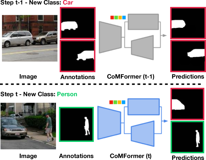
Figure 1: Illustration of our model, CoMFormer, operating in continual segmentation. Relying on the mask classification paradigm, it is able to cope with both continual semantic and panoptic segmentation without any modification by predicting masks for both old (e.g. car in red) and new (e.g. person in green) classes. The figure reports two classes and no “stuff” (e.g. road, building) only for illustration purposes.

Despite tremendous progress in image segmentation, the current approaches are trained on a static dataset with a predefined set of classes. Whenever an update of the model is required to fit new classes, the common solution is to train a model from scratch on the union of the old and new class data. A computationally more efficient solution would be to fine-tune the existing model solely on the new class data. Unfortunately, this approach would cause a catastrophic forgetting [21] of the old classes on which the model performance would be extremely degraded.

The problem of updating the knowledge of the model over time is typically referred as continual learning. It has been traditionally studied in the context of image classification [33, 29, 43, 45, 17, 19] and is gaining attention on the segmentation task [39, 4, 15, 59, 3] due to the more realistic applications and the additional challenges it introduces, such as the background shift [4]. However, current state-of-the-art methods mainly focus on semantic segmentation and are not designed to work in other segmentation tasks, strongly limiting their application in the real world.

In this paper, we design the first method operating in both continual semantic and panoptic segmentation, as illustrated in Fig. 1. Our method, CoMFormer (Continual MaskFormer), takes inspiration from recent transformer architectures [12, 11], approaching segmentation as a mask classification problem. Instead of predicting a class probability for each pixel, as in previous semantic segmentation works [37, 9], it predicts a set of binary masks, each associated with a single class prediction, effectively addressing both segmentation tasks without any modification in the training architecture and procedure. Differently from previous works [12, 11], however, CoMFormer forces the output binary masks to be mutually exclusive to one another: a pixel can only be predicted by a single binary mask to prevent having several masks classifying the same pixel with different classes. This behavior is crucial in continual learning to reduce the interference among old and new classes.

Furthermore, CoMFormer introduces a novel adaptive distillation loss to alleviate forgetting. It enforces consistency of the model’s classification predictions across learning steps only when it is useful to remember old classes, ensuring a better tradeoff between rigidity (not forgetting old classes) and plasticity (learning efficiently new classes). Finally, since at each training iteration the dataset reports annotations only for the current classes, we design a mask-based pseudo-labeling technique to generate annotations for the old classes, effectively alleviating forgetting. To reduce the noise, we consider the prediction confidence and we avoid interference with ground-truth annotations.

We validate CoMFormer on both continual segmentation tasks. For panoptic segmentation, we define a new benchmark relying on the challenging ADE20K where we demonstrate that CoMFormer largely outperforms all previous baselines. On semantic segmentation, we show that CoMFormer outperforms the existing state-of-the-art methods on every setting of the large-scale ADE20K benchmark.

To sum up, the contributions of this paper are as follows:

• We introduce continual panoptic segmentation which has real-world impacts in addition to being significantly more challenging than previous benchmarks.

• We propose CoMFormer to tackle both continual panoptic and semantic segmentation. To avoid forgetting, we design a novel adaptive distillation and an efficient mask-based pseudo-labeling strategy.

• Through extensive quantitative and qualitative benchmarks, we showcase the state-of-the-art performance of our model on both continual segmentation tasks.

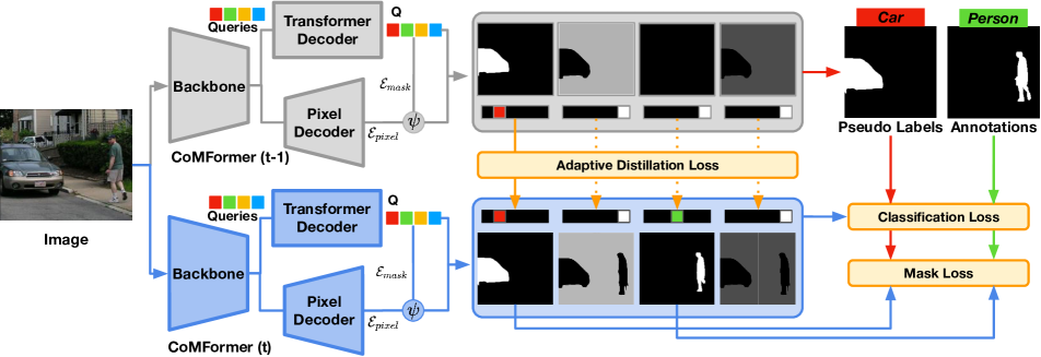
Figure 2: Overview of CoMFormer. At learning step t, both the current (bottom) and old (top) models output, for each input query, a pair made of a class probability distribution and a binary mask. While learning the new class (person), we regularize the current model to prevent forgetting the old classes (car) by: (i) generating pseudo-labels for the old classes present in the image and (ii) by applying an adaptive distillation loss that reweights the contribution of each output based on the information it carries on the old classes. $\psi$ indicates the dot product between the mask embeddings $\mathcal{E}_{mask}$ and the pixel embeddings $\mathcal{E}_{pixel}$ followed by the softmax activation.

2 Related Works

Semantic and Panoptic Segmentation.

The two tasks have been traditionally treated separately, with specialized architectures proposed for either one or the other task, without interoperability. Semantic segmentation has been traditionally addressed as a per-pixel classification task. Fully-convolutional network [37] dominated the field by aggregating long-range dependencies in the features map [8, 9, 60] and exploiting contextual information [22, 24, 58, 61, 57]. Recently, transformers [26, 54, 46] are replacing convolutions by integrating long-range dependencies at every layer. Panoptic segmentation [28] has been proposed to unify semantic and instance segmentations. Initially, methods proposed to combine each task-specific architectures [10, 27, 32, 42] or defined new specialized architectures and objective functions for the panoptic task [1, 50, 51], drifting from a general solution for all the segmentation tasks. Recently, methods addressing segmentation as a mask classsification problem [50, 56, 11, 12] have been proposed, introducing a transformer architecture able to solve multiple tasks at once. MaskFormer [12] was the first to propose a single architecture to address both panoptic and semantic segmentation. Mask2Former [11] improves it by adopting multi-scale features, masked attention and optimization tricks. Concurrently, kMaX-DeepLab [56] extended [50] proposing to reformulate the cross-attention as a clustering process. Despite their effectiveness in standard training setting, these methods suffer from catastrophic forgetting. In this work, we aim to extend their capability and we propose CoMFormer to learn to segment new classes over time.

Continual Segmentation.  Continual learning is a long-standing field addressing the problem of learning new knowledge over time while avoiding catastrophic forgetting [21, 47, 44]. Traditionally, it has been studied in the context of image classification [43, 33, 29, 45, 17, 6, 55, 19] but there is a growing interest in its applications in segmentation [39, 4, 5, 15, 2, 16, 40, 38, 59, 3]. Continual semantic segmentation introduces additional challenges, as pointed out by [4]. In particular, considering the task as a per-pixel classification problem, catastrophic forgetting is exacerbated by the background shift, where old classes pixels are treated as background in following training steps. [4] proposed a revision of the standard knowledge distillation framework to deal with it. [17, 39] introduced a distillation loss preserving the representation at feature level while [38] proposed an approach using old classes’ examples to alleviate forgetting. Recently, [59] presented a technique that decouples learning the representation of the new classes while freezing the representation for the old ones. Differently from previous work, we extend the benchmarks to solve both semantic and the more challenging panoptic segmentation task.

Continual Learning with Transformers.  Recent progresses made using tranformers for computer vision [14, 49, 48, 36] attracted the attention of the continual learning community [19, 53, 52]. In particular, DyTox [19] proposed to specialize the architecture on each task using a different task-specific token. Learning-to-Prompt [53] stores a pool of prompts that are employed to condition the whole forward execution of the patch tokens. To the best of our knowledge, transformers have been evaluated only in continual learning for image classification [19, 31] and we are the first to use them in the continual segmentation task.

3 CoMFormer

3.1 Problem Definition

The goal of image segmentation is to learn a model able to (i) partition the image into a set of N regions represented by binary masks and (ii) produce a class-probability distribution associated with each region. The differences among segmentation tasks rely on the semantics of the masks: semantic segmentation groups all the pixels of a class while panoptic segmentation distinguishes different object instances. In the following, we provide a general formulation for the two tasks since they only differ in the construction of the binary masks in the dataset.

Continual segmentation aims to train the model in multiple learning steps $t=1,\dots,T$, introducing at every step a new set of classes. Formally, during the learning step $t$ a dataset $D_{t}$ consisting of a collection of image and label pairs is provided. The label of each image takes the form of a set of $N^{gt}$ ground truth segments $z^{gt}\{(c_{i}^{gt},m_{i}^{gt})|c_{i}^{gt}\in\mathcal{K}^{t},m_{i}^{gt}\in\{0,1\}^{H\times W}\}_{i=1}^{N^{gt}}$ where $c_{i}^{gt}$ is the ground-truth class and $m_{i}^{gt}$ is binary mask $m^{gt}$, $\mathcal{K}^{t}$ is the set of classes introduced at step $t$, and $H$, $W$ are the height and width of the images. The goal of training step $t$ is to learn a model able to predict segments for all the seen classes $\mathcal{K}^{1:t}$.

We note that the dataset only contains annotations for the new classes $\mathcal{K}^{t}$ while not reporting ground-truth segments for old $\mathcal{K}^{1:t-1}$ or future $\mathcal{K}^{t+1:T}$ classes. Moreover, differently from previous works [4], old and future class segment annotations are simply absent during training rather than being collapsed into an artificial background class.

3.2 CoMFormer Architecture

To solve semantic and panoptic segmentation tasks within a single method, we take inspiration from MaskFormer architectures [12, 11] considering segmentation a mask classification problem. It consists in predicting for each image a set of $N$ pairs made of a class prediction and a binary mask. Formally, the output of a CoMFormer is $z=\{(p_{i},m_{i})\}_{i=1}^{N}$, where $p_{i}$ represents a class probability distribution over the seen classes, i.e. $p_{i}\in\Delta^{K^{t}+1}$ with $K^{t}=|\mathcal{K}^{1:t}|$, and $m_{i}$ is a binary mask such that $m_{i}\in[0,1]^{H\times W}$. We note that $p_{i}$ contains an additional “no object” class (denoted $\varnothing$) to indicate that the mask does not correspond to any of the known $\mathcal{K}^{1:t}$ categories.

To obtain such output, the CoMFormer architecture, showcased in Fig. 2, is made of three components: (i) a backbone that extracts feature embeddings $\mathcal{E}_{feat}$, (ii) a transformer decoder that takes as input N learnable queries and $\mathcal{E}_{feat}$ to output $N$ per-segment embeddings $Q$, (iii) a pixel decoder that takes $\mathcal{E}_{feat}$ as input and extracts per-pixel embeddings $\mathcal{E}_{pixel}$. The output class probabilities $\{p_{i}\in\Delta^{K^{t}+1}\}_{i=1}^{N}$ are obtained by applying a linear classifier on $Q$, which is enlarged as new classes are presented. We obtain the mask predictions $m_{i}$ combining $Q$ and $\mathcal{E}_{pixel}$: first $Q$ is passed into a 2-layer MLP to obtain N mask embeddings $\mathcal{E}_{mask}$ and we then compute the dot product between the $i$-th mask embedding and the pixel embeddings, followed by the softmax activation: $m_{i}[h,w]=\text{softmax}(\mathcal{E}_{mask}[:,i]^{T}\cdot\mathcal{E}_{pixel}[:,h,w])$.

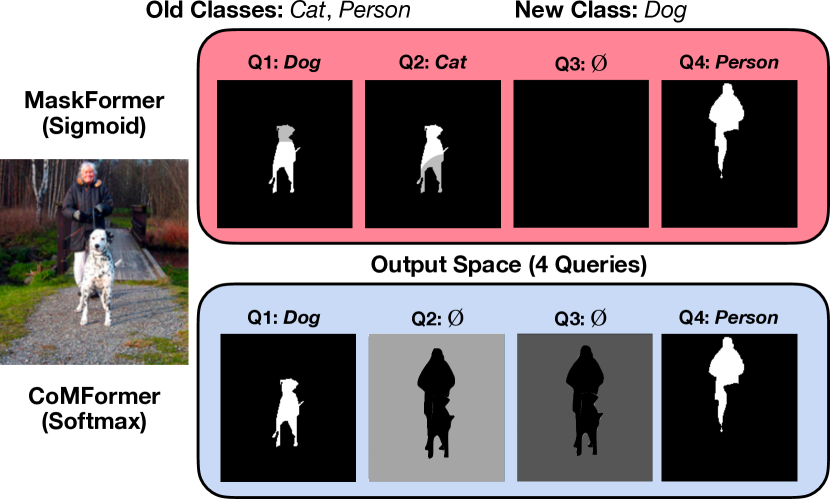
Figure 3: Illustration of the mask predictions between sigmoid and softmax. MaskFormer has overlap across masks (e.g. in Query 1 and 2) predicted either as old or new classes, while CoMFormer avoids the issue using the softmax activation.

We point out that employing the softmax contrasts sharply with MaskFormers [12, 11], which use sigmoid activation to get the mask predictions. Using the sigmoid activation would result in the overlap of many masks on a single pixel, each potentially belonging to a distinct class, as seen in Fig. 3. This is particularly important in the context of continual learning, when the model may predict two similar masks associated with two distinct classes (e.g. cat and dog classes in Fig. 3) thereby generating interference among old and new classes and degrading the model’s performance.

3.3 Learning without Forgetting

To learn new classes, a simple solution is to fine-tune the model on the new dataset. However, because it lacks annotations for old classes, this operation results in catastrophic forgetting [21]. To alleviate the issue, we introduce two techniques for avoiding forgetting: an adaptive distillation loss and a mask-based pseudo-labeling strategy.

Adaptive Distillation Loss.  A common strategy to mitigate forgetting adopted by continual semantic segmentation approaches [4, 39, 15] is to distill the knowledge coming from the old model in the new one, either in form of features [15, 39] or as classification probabilities [4]. We take inspiration from the latter solution and we design a novel distillation loss tailored to the CoMFormer architecture. In particular, analyzing the two components constituting the output space, we find the mask prediction being robust to forgetting while the classification part is heavily affected (see Tab. 5). For this reason, we focus on the output class probabilities to design our distillation loss.

An adaptation of standard knowledge distillation works [4] would force the new model to mimic the old model probabilities over all the N outputs, independently from their content. Formally, given the set of N probability distributions $\{p_{i}^{o}\}_{i=1}^{N}$ coming from the old model, a standard distillation loss is computed as

$$\mathcal{L}_{KD}=-\frac{1}{N}\sum_{i=1}^{N}\sum_{k=1}^{K^{t-1}+1}p_{i}^{o}(k)\log\frac{\tilde{p}_{i}(k)}{p_{i}^{o}(k)},$$ (1)

where $K^{t-1}+1$ is the $\varnothing$ class and $\tilde{p}_{i}(k)$ represents the unbiased probability distribution of $i$-th output for class $k$:

$$\tilde{p}_{i}(k)=\begin{cases}\sum_{j\in\mathcal{K}^{t}}p_{i}(j)+p_{i}(\varnothing)&\text{if $k=\varnothing$},\\ p_{i}(k)&\text{otherwise}.\\ \end{cases}$$ (2)

Note that, similarly to [4], it forces the sum of the model new class ($\mathcal{K}^{t}$) and the “no object” class ($\varnothing$) probabilities to be similar to the old model $\varnothing$ probability.

However, not every output probability brings relevant information: most of them are predicted as “no object” ($\varnothing$) and thus they do not carry enough details to remember the old classes while reducing the relative importance of the other outputs probabilities. For this reason, we re-weight their contribution based on the probability of not being $\varnothing$. Formally, we define our adaptive distillation loss as

$$\mathcal{L}_{AD}(p,p^{o})=-\sum_{i=1}^{N}\frac{\omega_{i}}{\sum_{i=1}^{N}\omega_{i}}\sum_{k=1}^{K^{t-1}+1}p_{i}^{o}(k)\log\frac{\tilde{p}_{i}(k)}{p_{i}^{o}(k)},$$ (3)

where the weighting coefficient is $\omega_{i}=(1-p_{i}^{o}(\varnothing))^{2}$. Note that, with this formulation, we effectively reduce the contributions of outputs that bring small information about the old classes ($p_{i}^{o}(\varnothing)\approx 1$), while we increase the contribution of important ones (where $p_{i}^{o}(\varnothing)\approx 0$).

Mask-based Pseudo-labeling Strategy.  Forgetting is effectively reduced by the adaptive distillation loss but we are not, however, taking advantage of the presence of the old classes that are unlabeled in the dataset. We propose using the old model predictions to recognize old class segments and generate pseudo-labels to make efficient use of this information and improve the knowledge of past classes.

A simple strategy consists in considering the N output pairs coming from the old model independently and using all the pairs for which the predicted class is not $\varnothing$ as pseudo-labels. This strategy, however, does not consider two aspects: there may be pairs where the class is different from $\varnothing$ but (i) the mask substantially overlaps with a ground-truth segment, or (ii) the mask is noisy and has low confidence.

To overcome these issues, we propose a mask-based pseudo-labeling strategy that jointly considers the mask and class prediction confidences to avoid noisy labels and overlaps with the existing annotations. We define the model confidence as the multiplication among the class and mask probabilities. Formally, we compute the confidence for the $i$-th output as $q_{i}=p^{max}_{i}\cdot m^{o}_{i}\in[0,1]^{H\times W}$, where $p^{max}_{i}=\max_{k=1}^{K^{t-1}}p^{o}_{i}(k)$ and $m^{o}_{i}$ is the binary mask predicted by the old model. Note that we do not consider the $\varnothing$ class in the $\max$ operation. We denote the pseudo-class $c^{ps}_{i}=\operatorname*{argmax}_{k=1}^{K^{t-1}}p^{o}_{i}(k)$ and we generate the pseudo-mask $m_{i}^{ps}$ considering two criteria: (i) there should be no overlap between the pseudo-mask and the ground-truth segments and (ii) to be included in a pseudo-mask, the confidence on a pixel should be maximum over all outputs. Formally, denoting the binarization of the predicted mask as $m_{i}^{bin}=m_{i}>0.5$ and the union of the ground-truth segments $m^{gt}_{all}=\sum_{i=1}^{N^{ps}}m_{i}^{gt}$, we generate the pseudo-mask as

$$\small m_{i}^{ps}[h,w]=\begin{cases}m_{i}^{bin}[h,w]&\text{if}\;i=\operatorname*{argmax}_{j=1}^{N}q_{j}[h,w]\\ &\;\;\;\;\text{and}\;m^{gt}_{all}[h,w]=0,\\ 0&\text{otherwise}.\\ \end{cases}$$ (4)

Indeed, not all pseudo-mask should be included in the set of pseudo-labels. There may be pseudo-masks where no pixel is active, i.e. it is all zeros, or where the pseudo-mask contains only a small fraction of the original mask. For these reasons, we construct the set of pseudo-labels $z^{ps}=\{(c^{ps}_{i},m^{ps}_{i})\}_{i=1}^{N^{ps}}$ such that we include in $z^{ps}$ only the pseudo-masks that retain at least half of the pixels w.r.t. the binary mask $m_{i}^{bin}$ and that have at least one active pixel.

We denote the final annotation set $\bar{z}=\{\bar{c}_{i},\bar{m}_{i}\}_{i=1}^{\bar{N}}$ as the union of the ground-truth labels $z^{gt}$ and the pseudo-labels $z^{ps}$, i.e. $\bar{z}=z^{gt}\cup z^{ps}$ and $\bar{N}=N^{gt}+N^{ps}$.

Overall training loss.  To train CoMFormer, a one-to-one matching $\sigma$ between the model predictions $z$ and the annotation set $\bar{z}$ is required. Following standard practices [1, 11], we employ the Hungarian matching algorithm [30] and we search for the matching $\sigma$ that minimize the assignment cost computed as $-p_{i}(\bar{c}_{j})\cdot Dice(m_{i},\bar{m}_{j})$, where $Dice$ indicates the Dice coefficient [13]. We assume the size of the prediction set to be larger than the annotations set (i.e. $N>\bar{N}$) and to obtain a one-to-one matching we pad the annotations with “no object” tokens $\varnothing$.

Once the best matching $\sigma$ has been found, we define the overall training loss as:

$$\mathcal{L}=\mathcal{L}_{Seg}(z,\bar{z})+\lambda_{D}\mathcal{L}_{AD}(p,p^{o}),$$ (5)

where $\lambda_{D}$ is a trade-off hyper-parameter and

$$\mathcal{L}_{Seg}(z,\bar{z})=\sum_{j=1}^{\bar{N}}[-\alpha(1-p_{\sigma(j)}(\bar{c}_{j}))^{\gamma}\log p_{\sigma(j)}(\bar{c}_{j})+$$ (6)

$$+\lambda_{mask}\mathds{1}_{\bar{c}_{j}\neq\varnothing}\mathcal{L}_{mask}(m_{\sigma(j)},\bar{m}_{j})].$$

We note that the first term in $\mathcal{L}_{Seg}$ indicates the focal loss [34], where $\alpha$ and $\gamma$ are hyper-parameters. Finally, $\mathcal{L}_{mask}$ is the sum of dice and cross-entropy losses, and $\lambda_{mask}$ is a hyper-parameter. We note that $\mathcal{L}_{mask}$ is computed only for valid segments, i.e. where $\bar{c}_{j}\neq\varnothing$.

4 Experiments

	100-50 (2 tasks)				100-10 (6 tasks)				100-5 (11 tasks)
Method	1-100	101-150	all	avg	1-100	101-150	all	avg	1-100	101-150	all	avg
FT	0.0	25.8	8.6	24.8	0.0	2.9	1.0	7.9	0.0	1.3	0.4	4.6
MiB	35.1	19.3	29.8	35.4	27.1	10.0	21.4	29.1	24.0	6.5	18.1	25.6
PLOP	41.0	26.6	36.2	38.6	30.5	17.5	26.1	32.9	28.1	15.7	24.0	30.5
CoMFormer	41.1	27.7	36.7	38.8	36.0	17.1	29.7	35.3	34.4	15.9	28.2	34.0
Joint	43.2	32.1	39.5	—	43.2	32.1	39.5	—	43.2	32.1	39.5	—

Table 1: Continual Panoptic Segmentation results on ADE20K dataset in PQ considering multiple training protocols.

		100-50 (2 tasks)				100-10 (6 tasks)				100-5 (11 tasks)
Backbone	Method	1-100	101-150	all	avg	1-100	101-150	all	avg	1-100	101-150	all	avg
DeepLab-v3 [9]	MiB [4]	40.5	17.2	32.8	37.3	38.3	11.3	29.2	35.1	36.0	5.7	26.0	32.7
	PLOP [15]	41.9	14.9	32.9	37.4	40.5	14.1	31.6	36.6	39.1	7.8	28.8	35.3
	RCIL [59]	42.3	18.8	34.5	—	39.3	17.6	32.1	—	38.5	11.5	29.6	—
Per-Pixel	MiB	40.3	24.0	34.8	37.5	35.1	14.0	28.1	34.0	33.3	15.2	27.3	33.1
	PLOP	40.2	20.2	33.5	36.9	32.6	13.7	26.3	32.4	33.3	9.4	25.4	32.8
Mask-based	FT	0.0	26.7	8.9	26.4	0.0	2.3	0.8	8.5	0.0	1.1	0.3	4.2
	MiB	37.0	24.1	32.6	38.3	23.5	10.6	26.6	29.6	21.0	6.1	16.1	27.7
	PLOP	44.2	26.2	38.2	41.1	34.8	15.9	28.5	35.2	33.6	14.1	27.1	33.6
	CoMFormer	44.7	26.2	38.4	41.2	40.6	15.6	32.3	37.4	39.5	13.6	30.9	36.5
	Joint	46.9	35.6	43.1	—	46.9	35.6	43.1	—	46.9	35.6	43.1	—

Table 2: Continual Semantic Segmentation results on the ADE20K dataset in mIoU considering multiple training protocols. We report the numbers published by the original papers on DeepLab-v3 [9]. The remaining results are based on our re-implementation (see Sec. 4.2).

4.1 Dataset and Settings

We start from the widely adopted continual semantic segmentation benchmark defined in [4] and we extend it to the newly proposed continual panoptic segmentation using a modified Continuum library [18]. We compare our novel model on the large-scale ADE20K [62] dataset since it supports both semantic and panoptic segmentation tasks. This challenging dataset contains 150 classes, divided into 100 “things” and 50 “stuff” categories. This dataset represents a wide variety of scenes, both interior and exterior, with images featuring an average of 9.9 classes, while other datasets like COCO [35] only have an average of 3.5 classes.

Continual Learning Protocols.  Previous continual semantic segmentation works [15, 4] describe a training protocol to assess the performance on multiple continual learning steps. In particular, [4] proposed three protocols for ADE20K with different numbers of tasks: (i) the 100-50 consists of two tasks, the first of 100 and the second of 50 classes; (ii) the 50-50 consists of three tasks of 50 classes; (iii) the 100-10 consists on 6 tasks, the first on 100 classes followed by 5 tasks of 10 classes. In addition, we use the 100-5 introduced in [15], consisting of 11 tasks, the first of 100 classes followed by 10 tasks of 5 classes. To divide the images into different tasks, we follow the splits provided by [4] for 100-50, 100-10, 50-50 for both semantic and panoptic segmentation. In particular, they ensured that each image appears only on a unique task. Differently, for the 100-5 we use the split proposed by [15], where the same image may appear on multiple tasks. We report the results of the 50-50 setting for both semantic and panoptic segmentation in the supplementary material.

Metrics.  We compare the different models using the mean Intersection over Union (mIoU) on semantic segmentation [20] and Panoptic Quality (PQ) on panoptic segmentation [28]. PQ is the product of two components: Segmentation Quality (SQ) which considers the IoU between the correctly classified segments, and Recognition Quality (RQ) which only considers the classification accuracy. For both tasks, we report the metric after the last step $T$ on the first classes ($C^{1}$), for the added classes ($C^{2:T}$), and for all the classes (all). We also report the average of the final performance on all seen classes after each step (avg) following [15].

4.2 Baselines

We benchmark our model against the state-of-the-art methods: MiB [4], PLOP [15], and RCIL [59]. In semantic segmentation, we report them with the original DeepLab-v3 segmentation architecture [9]. In addition, for a fair comparison, we report MiB and PLOP using the CoMFormer architecture. In particular, we implement the methods in two versions: (i) we replace the CoMFormer losses with a per-pixel cross-entropy loss on the dot product between mask and class logits and we apply the continual learning methods on that baseline (we refer to this as Per-Pixel), and (ii) by applying the distillation losses directly on the classification head of the CoMFormer architecture (Mask-based). We note that the first version cannot be applied to panoptic segmentation, since the task does not support the use of per-pixel losses. For PLOP, we apply its distillation loss local-POD on the intermediate features of the segmentation backbone, as in the original paper, and we use the pseudo-labeling strategy proposed in Sec. 3. RCIL was not re-implemented since it is not possible to extend their approach to non-convolutional architectures like ours. We include a naive finetuning (FT) without any capabilities for continual learning. Finally, we also report an upper bound (Joint) that is trained in the traditional segmentation setting. We made our best effort to find the most suitable hyper-parameters for all the baselines.

4.3 Implementation Details

Architecture.  Following the previous benchmarks [4, 15] we use as backbone a ResNet101 [23] on semantic segmentation and we propose to use a ResNet50 [23] for panoptic segmentation. For both tasks, we use the pixel decoder and the transformer decoder proposed in [11] with 9 layers in total and $N=100$ queries. In addition, we adopt all the improvements introduced in [11]: masked attention, multi-scale features, and their optimization improvements. We report the performance of single-scale inference.

Training parameters.  We follow the Mask2Former [11] hyper-parameters and we use AdamW [25] optimizer with an initial learning rate of $0.0001$ for the first step ($t=0$) and $0.00005$ in the following ($t>0$). A learning rate multiplier of 0.1 is applied to the backbone and we follow a polynomial learning rate schedule. We use weight decay of $0.05$. We train the model for 160K iterations in the first step and 400 iterations per class in the following (e.g. learning 50 classes we train for $50\times 400=20000$ iterations). For semantic segmentation, we use a crop size of 512 and a batch size of 16. For panoptic segmentation, we use a crop size of 640 and a batch size of 8. For both, we use the standard random scale jittering between 0.5 and 2.0, random horizontal flipping, random cropping, as well as random color jittering as data augmentation [12]. We set $\alpha=20$, $\gamma=2$, and $\lambda_{mask}=5.0$. $\lambda_{D}$ is set to $1$ for 100-50 and to $10$ in the 100-10 and 100-5. Finally, following the standard protocol of continual learning [4, 15] we do not store any image of previous steps and we do not use rehearsal learning.

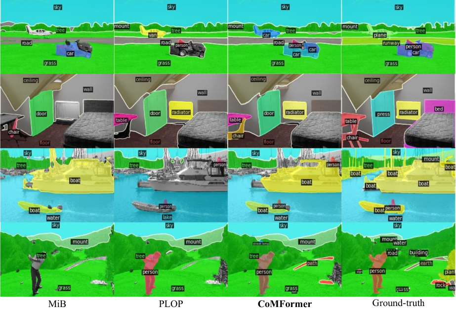
Figure 4: Qualitative results of CoMFormer v.s. MiB and PLOP on the 100-10 continual panoptic segmentation setting on ADE20K.

4.4 Continual Panoptic Segmentation

Tab. 1 reports the results on the new continual panoptic segmentation benchmark. CoMFormer exceeds all the baselines by a significant margin. Considering the 100-50, we can see that CoMFormer outperforms MiB on both old (+6 PQ) and new (+8.4 PQ) classes and PLOP on new classes (+1.1 PQ). Considering a longer sequence of tasks (100-10 and 100-5), we can see that the gap between CoMFormer and the other methods becomes more significant, especially in the old classes. In 100-10, it surpasses MiB and PLOP respectively by 8.9 and 5.5 PQ in old classes, while in the new classes it exceeds MiB by 7.1 and is comparable to PLOP. In the 100-5, it outperforms MiB and PLOP on both old (+10.4 and +6.3 PQ) and new classes (+9.4 and +0.2 PQ). Finally, we note that CoMFormer obtains performance close to the Joint baseline in the 100-50 setting, suffering a drop of only 2.1 PQ on the old classes and 4.4 PQ on the new ones. In the other settings, the gap is still relevant, indicating that learning from multiple training steps is still a very challenging task.

In Fig. 7, we report a qualitative comparison with the baselines in the 100-10 setting using randomly chosen images. We can see that our method is able to maintain better the previous knowledge by precisely segmenting all the classes in the image; for example, w.r.t. to PLOP, our method correctly segments the chair in the second row and the boat in the third row. We can note a common error: models correctly segment but misclassify objects in the image, like the plane classified as car in the first row or the press classified as a door in the third row.

4.5 Continual Semantic Segmentation

We report the comparison with state-of-the-art methods in continual semantic segmentation in Tab. 2. CoMFormer achieves the best results on every setting, surpassing both methods based on DeepLab-v3 [9] and baselines implemented upon the same architecture. In particular, we can see that CoMFormer outperforms the best state-of-the-art method (RCIL [59] by 3.9% on the 100-50, by 0.2% on 100-10, and by 1.3% on the 100-5. Moreover, note that we always improve the performance on the old classes and the avg across different learning steps. In addition, CoMFormer exceeds all the implemented baselines. Comparing CoMFormer with PLOP (Mask-based), we can see that it obtains a substantial performance improvement, especially considering scenarios with longer training protocols: CoMFormers achieves 30.9% (32.3%) on the all metrics, while PLOP only 27.1% (28.5%) on the 100-5 (100-10) setting. Furthermore, the results confirm that improvements are not led by the newer architecture. Per-Pixel baselines achieve only similar or even lower performance than their counterparts. MiB (Per-Pixel), for example, slightly improves the one based on DeepLab-v3 on the 100-50 (+2.0% on all) and in the 100-5 (+1.3%) but its performance is slightly worse in the 100-10 (-1.1%). In addition, note that Per-Pixel baselines demonstrate a large performance drop in the old classes w.r.t. their counterpart, showing that, without employing a distillation strategy tailored to the architecture, it is difficult to maintain satisfactory results.

4.6 Ablation Studies

	Semantic - mIoU			Panoptic - PQ
Method	1-100	101-150	all	1-100	101-150	all
	100-50 (2 tasks)
Mask2Former	44.3	26.0	38.1	37.9	24.5	33.4
CoMFormer	44.7	26.2	38.4	41.1	27.7	36.7
	100-10 (6 tasks)
Mask2Former	38.7	15.7	31.0	30.2	10.8	23.7
CoMFormer	40.6	15.6	32.3	36.0	17.1	29.7
	100-5 (11 tasks)
Mask2Former	32.6	13.7	26.3	25.9	5.6	19.1
CoMFormer	39.5	13.6	30.9	34.4	15.9	28.2

Table 3: Comparison between CoMFormer and Mask2Former [11] in continual semantic and panoptic segmentation. We apply to Mask2Former our mask-based pseudo-labeling strategy and the adaptive distillation loss for a fair comparison.

Mask2Former vs CoMFormer.  In Tab. 3, we compare the proposed CoMFormer against Mask2Former [11]. In particular, to fairly compare the two methods, we add our adaptive distillation loss and the pseudo-labeling strategy to Mask2Former. Considering semantic segmentation, CoMFormer achieves better results on the old classes (on average 3% mIoU), while the two methods obtain comparable results on the new classes. On panoptic segmentation, CoMFormer exceeds Mask2Former in all the classes with a considerable gap (6 PQ on both old and new classes on average). We conclude that a vanilla MaskFormer architecture is not suited to continual learning because it suffers from forgetting, while CoMFormer outperforms it in any setting.

			100-50 (2 tasks)			100-10 (6 tasks)
PS	KD	AD	1-100	101-150	all	1-100	101-150	all
-	-	-	0.0	25.8	8.6	0.0	2.9	1.0
-	-	✓	28.4	15.3	24.0	23.0	9.1	18.4
✓	-	-	40.7	26.3	35.9	30.1	17.2	25.8
✓	✓	-	40.5	28.1	36.4	30.2	17.6	26.0
✓	-	✓	41.1	27.7	36.7	36.0	17.1	29.7

Table 4: Ablation of the different key components of our CoMFormer architecture. We report the PQ on the 100-50 and 100-10 panoptic settings. PS: Pseudo-labeling; AD: adaptive distillation Eq. 3; KD: standard distillation Eq. 1

Method components.  We investigate the benefit of each method component in Tab. 4, reporting the results in PQ on the 100-50 and 100-10 settings in panoptic segmentation. Without applying any regularization technique, the performance on old classes drops to 0, denoting that it is important to deal with forgetting. Both the adaptive distillation loss (AD) and the pseudo-labeling strategy (PS) lead to improvement in the old classes when applied independently. However, we obtain the best results when combining them, especially considering the 100-10 scenario, where the old classes are improved by 5.8 PQ and the final performances of 3.9 PQ. Finally, the table shows that weighting the queries based on their semantic content is essential to improve performance: comparing a standard distillation (KD Eq. 1) with our adaptive distillation (AD Eq. 3), we largely improve the performance on both settings: +0.3 PQ in 100-50 and +3.7 PQ in 100-10 considering all classes.

	100-50 (2 tasks)			100-10 (6 tasks)
Method	RQ	SQ	PQ	RQ	SQ	PQ
MiB	36.8	73.0	29.8	26.4	55.5	21.4
PLOP	43.8	79.1	36.2	31.7	61.1	26.1
CoMFormer	44.4	79.6	36.7	36.2	73.4	29.7
Joint	47.6	79.0	39.5	47.6	79.0	39.5

Table 5: Panoptic metrics analysis. We report Recognition Quality (RQ), Segmentation Quality (SQ), and Panoptic Quality (PQ) over all the classes after the last step.

Forgetting in CoMFormer.  To investigate the reason for the forgetting, we considered separately the Recognition Quality (RQ) and the Segmentation Quality (SQ) in panoptic segmentation. RQ measures how well the model is able to classify segments, while SQ considers the precision of the segmentation. Note that, as reported in [28], SQ and RQ are not independent since SQ is computed only on segments correctly classified. The results on the 100-50 and 100-10 are reported in Tab. 5. The table clearly shows that, as hypothesized in Sec. 3.3, forgetting happens heavily on the classification ability while it is less marked on the segmentation ability of the model. CoMFormer, in fact, without providing regularization losses on the mask prediction, is able to match the segmentation ability of the Joint upper bound on the 100-50 and it gets close results on the 100-10 (-5.6). In addition, it is evident that classification ability is heavily affected by forgetting. CoMFormer has a gap with Joint of 3.2 and 11.4 RQ respectively in the 100-50 and 100-10. We note that, however, other baselines are more affected by forgetting, showcasing even larger gaps.

5 Conclusion

In this paper, we extend the task of continual learning beyond semantic segmentation by introducing the challenging and realistic continual panoptic segmentation setting. We propose CoMFormer, a strategy to address segmentation as a mask classification problem exploiting the properties of transformers to tackle both semantic and panoptic segmentation tasks. The extensive quantitative results highlight that CoMFormer outperforms all previous methods, both in semantic and panoptic segmentation, under a unified paradigm. In future work, we aim to extend the benchmark to instance segmentation to show that CoMFormer can be employed to address any continual segmentation task.

Acknowledgments. Fabio Cermelli acknowledges travel support from ELISE (GA no 951847). We acknowledge that the research activity was carried out using the IIT HPC infrastructure.

Appendix

Appendix A Additional quantitative results

50-50 in Continual Panoptic Segmentation.  In Tab. 6 we report additional experiments on Continual Panoptic Segmentation on the 50-50 setting where we perform three tasks of 50 classes. CoMFormer outperforms all the baselines, obtaining the best results on both old and new classes. In particular, we can see that it exceeds the best competitor, PLOP, by 0.5 PQ in the old classes and 0.2 PQ in the new ones. When comparing with MiB, however, we can see that the gap is more relevant: +11.6 PQ on old classes and +10.2 on the new ones. Finally, we can see that CoMFormer obtains a small performance gap with the Joint baselines, which is more relevant for the new classes (-7.6 PQ).

	50-50 (11 tasks)
Method	1-50	51-150	avg	all
FT	0.0	14.3	23.1	9.5
MiB	33.6	16.3	31.8	22.1
PLOP	44.7	26.3	37.9	32.4
CoMFormer	45.2	26.5	37.9	32.7
Joint	50.2	34.1	—	39.5

Table 6: Continual Panoptic Segmentation results on ADE20K dataset on 50-50 setting in PQ.

		50-50 (11 tasks)
Architecture	Method	1-50	51-150	avg	all
DeepLab-v3 [9]	MiB [4]	45.3	21.6	38.9	29.3
	PLOP [15]	48.6	21.6	39.4	30.4
	RCIL [59]	48.3	25.0	—	32.5
Per-Pixel	MiB	44.9	25.4	35.0	31.9
	PLOP	43.2	24.7	34.6	30.9
Mask-Based	FT	0.0	13.3	12.8	8.9
	MiB	24.6	19.4	25.8	21.1
	PLOP	48.1	26.6	36.5	33.8
	CoMFormer	49.2	26.6	36.6	34.1
	Joint	53.4	38.0	—	43.1

Table 7: Continual Semantic Segmentation results on ADE20K dataset on 50-50 setting in mIoU.

50-50 in Continual Semantic Segmentation.  Tab. 7 reports the additional results on the Continual Semantic Segmentation benchmark on the 50-50 setting in mIoU, comparing CoMFormer with previous works based on DeepLab [9] and our re-implementation based on the CoMFormer architecture, both in Per-Pixel and Mask-Based fashion. We observe that CoMFormer achieves a new state of the art. In particular, when comparing it with previous works, we can see that it outperforms the best baseline (RCIL) on both old (+0.9 mIoU) and new classes (+1.6 mIoU), for an overall improvement of 1.6 mIoU. Furthermore, CoMFormer also outperforms the baselines implemented on the same architecture: w.r.t. to Per-Pixel baselines, there is a relevant performance gap, especially regarding the old classes (CoMFormer 49.2 vs MiB 44.9 mIoU). Considering the Mask-Based baselines, CoMFormer shows the best performance, improving PLOP by 1.1 mIoU on the old classes and by 0.3 mIoU on all.

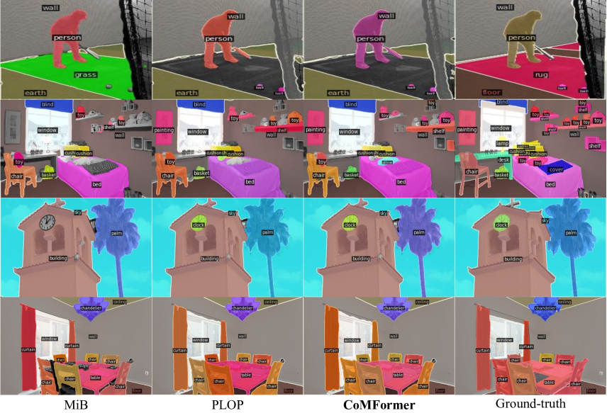
Figure 5: Qualitative results of CoMFormer v.s. MiB and PLOP on the 100-50 continual panoptic segmentation setting on ADE20K.

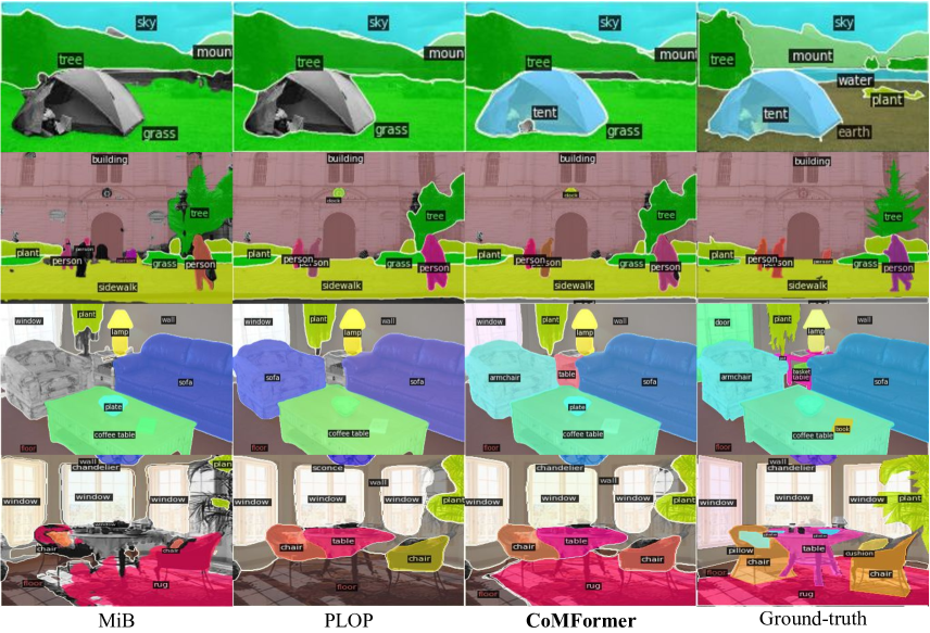
Figure 6: Qualitative results of CoMFormer v.s. MiB and PLOP on the 100-5 continual panoptic segmentation setting on ADE20K.

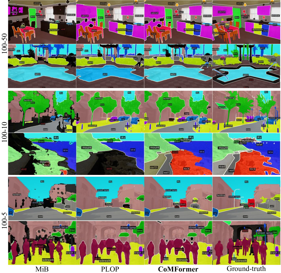
Figure 7: Qualitative results of CoMFormer v.s. MiB and PLOP on multiple settings of the continual semantic segmentation benchmark on ADE20K.

Appendix B Additional qualitative results

Continual Panoptic Segmentation.  Fig. 5 and Fig. 6 report additional qualitative results on, respectively, the 100-50 and 100-5 settings in continual panoptic segmentation, comparing CoMFormer with MiB and PLOP using images randomly sampled from the validation set. Considering the 100-50, we can see that PLOP and CoMFormer achieve visually similar results, while MiB struggles in segmenting every image object (for example, the clock in the third row). Differently, on the 100-5, CoMFormer visually outperforms the other baselines being able to correctly segment all the objects in the image (e.g. the tent in the first row, the table in the third row, and the rug in the fourth row). However, we note a common error across all the methods: some classes are correctly segmented but misclassified (e.g. grass instead of earth in the first row and window instead of door in the third). This error is less present in CoMFormer w.r.t. PLOP and MiB, as can be seen from the chandelier in the last row and the armchair in the third.

Continual Semantic Segmentation.  Fig. 7 reports the qualitative results for the 100-50, 100-10, and 100-5 settings of the continual semantic segmentation benchmark comparing CoMFormer with MiB and PLOP on images randomly sampled from the validation set. Considering the 100-50 setting, MiB is far worse than other baselines: it is not able to correctly segment the object in the image, achieving low performance. PLOP and CoMFormer achieve similar results, being able to segment all the objects in the images. Differently, on the 100-10 setting, the difference among methods becomes more evident: considering the second row, CoMFormer correctly segments the rock and the wall, while misclassifying the road with earth. However, both PLOP and MiB are not able to segment the image: the former is not able to report any segment in that area, while the latter segments incorrectly the area as mount. Finally, considering the 100-5 setting, we note that MiB achieves poor performance on both images, being unable to finely segment the image pixels. Comparing CoMFormer with PLOP, our model CoMFormer is able to segment more classes (e.g. the truck in the fifth row and the bag in the last row), obtaining better performances. Overall, the qualitative results confirm the quantitative findings, where CoMFormer outperforms the other methods, especially considering settings where multiple learning steps are performed. Those longer continual settings are more realistic and allows us to benchmark more efficiently what a truly lifelong learning agent should be.

Idx	Name	Thing	Idx	Name	Thing	Idx	Name	Thing
1	wall		51	refrigerator	✓	101	poster	✓
2	building		52	grandstand		102	stage
3	sky		53	path		103	van	✓
4	floor		54	stairs	✓	104	ship	✓
5	tree	✓	55	runway		105	fountain	✓
6	ceiling		56	case	✓	106	conveyer
7	road		57	pool	✓	107	canopy	✓
8	bed	✓	58	pillow	✓	108	washer	✓
9	windowpane	✓	59	screen	✓	109	plaything	✓
10	grass		60	stairway		110	swimming
11	cabinet	✓	61	river		111	stool	✓
12	sidewalk		62	bridge		112	barrel	✓
13	person	✓	63	bookcase	✓	113	basket	✓
14	earth		64	blind	✓	114	waterfall
15	door	✓	65	coffee	✓	115	tent	✓
16	table	✓	66	toilet	✓	116	bag	✓
17	mountain		67	flower	✓	117	minibike	✓
18	plant	✓	68	book	✓	118	cradle	✓
19	curtain	✓	69	hill		119	oven	✓
20	chair	✓	70	bench	✓	120	ball	✓
21	car	✓	71	countertop	✓	121	food	✓
22	water		72	stove	✓	122	step	✓
23	painting	✓	73	palm	✓	123	tank	✓
24	sofa	✓	74	kitchen	✓	124	trade	✓
25	shelf	✓	75	computer	✓	125	microwave	✓
26	house		76	swivel	✓	126	pot	✓
27	sea		77	boat	✓	127	animal	✓
28	mirror	✓	78	bar	✓	128	bicycle	✓
29	rug		79	arcade	✓	129	lake
30	field		80	hovel		130	dishwasher	✓
31	armchair	✓	81	bus	✓	131	screen	✓
32	seat	✓	82	towel	✓	132	blanket	✓
33	fence	✓	83	light	✓	133	sculpture	✓
34	desk	✓	84	truck	✓	134	hood	✓
35	rock	✓	85	tower		135	sconce	✓
36	wardrobe	✓	86	chandelier	✓	136	vase	✓
37	lamp	✓	87	awning	✓	137	traffic	✓
38	bathtub	✓	88	streetlight	✓	138	tray	✓
39	railing	✓	89	booth	✓	139	ashcan	✓
40	cushion	✓	90	television	✓	140	fan	✓
41	base	✓	91	airplane	✓	141	pier
42	box	✓	92	dirt		142	crt	✓
43	column	✓	93	apparel	✓	143	plate	✓
44	signboard	✓	94	pole	✓	144	monitor	✓
45	chest	✓	95	land		145	bulletin	✓
46	counter	✓	96	bannister	✓	146	shower	✓
47	sand		97	escalator		147	radiator	✓
48	sink	✓	98	ottoman	✓	148	glass	✓
49	skyscraper		99	bottle	✓	149	clock	✓
50	fireplace	✓	100	buffet	✓	150	flag	✓

Table 8: Class ordering of ADE20K [62] used in all reported experiments.

Appendix C Class Ordering

In Tab. 8 we report the class ordering of ADE20K that we used for all the reported experiments, following the previous benchmarks [4, 15]. Considering the 100-50, 100-10, and 100-5 settings, reported in the main paper, we note that 44 of the new classes are “things”, while the other 6 are “stuff”. While there is no difference between “things” and “stuff” in semantic segmentation, it is especially relevant in the panoptic segmentation task, where the goal is to separate in different segments multiple instances of the “things” classes, since it introduces additional challenges.

References

- [1] Nicolas Carion, Francisco Massa, Gabriel Synnaeve, Nicolas Usunier, Alexander Kirillov, and Sergey Zagoruyko. End-to-end object detection with transformers. In ECCV, pages 213–229. Springer, 2020.
- [2] Fabio Cermelli, Dario Fontanel, Antonio Tavera, Marco Ciccone, and Barbara Caputo. Incremental learning in semantic segmentation from image labels. In CVPR, pages 4371–4381, 2022.
- [3] Fabio Cermelli, Antonino Geraci, Dario Fontanel, and Barbara Caputo. Modeling missing annotations for incremental learning in object detection. In Proceedings of the IEEE/CVF Conference on Computer Vision and Pattern Recognition, pages 3700–3710, 2022.
- [4] Fabio Cermelli, Massimiliano Mancini, Samuel Rota Bulò, Elisa Ricci, and Barbara Caputo. Modeling the background for incremental learning in semantic segmentation. In Proceedings of the IEEE Conference on Computer Vision and Pattern Recognition (CVPR), 2020.
- [5] Fabio Cermelli, Massimiliano Mancini, Yongqin Xian, Zeynep Akata, and Barbara Caputo. Prototype-based incremental few-shot segmentation. In Proceedings of the British Machine Vision Conference (BMVC), 2021.
- [6] Arslan Chaudhry, Marc’Aurelio Ranzato, Marcus Rohrbach, and Mohamed Elhoseiny. Efficient lifelong learning with a-gem. In Proceedings of the International Conference on Learning Representations (ICLR), 2019.
- [7] Hongwei Chen, Laihui Ding, Fengqin Yao, Pengfei Ren, and Shengke Wang. Panoptic segmentation of uav images with deformable convolution network and mask scoring. In Twelfth International Conference on Graphics and Image Processing (ICGIP 2020), volume 11720, pages 312–321. SPIE, 2021.
- [8] Liang-Chieh Chen, George Papandreou, Iasonas Kokkinos, Kevin Murphy, and Alan L. Yuille. Deeplab: Semantic image segmentation with deep convolutional nets, atrous convolution, and fully connected crfs. In IEEE Transactions on Pattern Analysis and Machine Intelligence (TPAMI), 2018.
- [9] Liang-Chieh Chen, George Papandreou, Florian Schroff, and Hartwig Adam. Rethinking atrous convolution for semantic image segmentation. In arXiv preprint library, 2017.
- [10] Bowen Cheng, Maxwell D Collins, Yukun Zhu, Ting Liu, Thomas S Huang, Hartwig Adam, and Liang-Chieh Chen. Panoptic-deeplab: A simple, strong, and fast baseline for bottom-up panoptic segmentation. In CVPR, pages 12475–12485, 2020.
- [11] Bowen Cheng, Ishan Misra, Alexander G Schwing, Alexander Kirillov, and Rohit Girdhar. Masked-attention mask transformer for universal image segmentation. arXiv preprint arXiv:2112.01527, 2021.
- [12] Bowen Cheng, Alexander G. Schwing, and Alexander Kirillov. Per-pixel classification is not all you need for semantic segmentation. 2021.
- [13] Lee R. Dice. Measures of the amount of ecologic association between species. Ecology, 1945.
- [14] Alexey Dosovitskiy, Lucas Beyer, Alexander Kolesnikov, Dirk Weissenborn, Xiaohua Zhai, Thomas Unterthiner, Mostafa Dehghani, Matthias Minderer, Georg Heigold, Sylvain Gelly, Jakob Uszkoreit, and Neil Houlsby. An image is worth 16x16 words: Transformers for image recognition at scale. In Proceedings of the International Conference on Learning Representations (ICLR), 2021.
- [15] Arthur Douillard, Yifu Chen, Arnaud Dapogny, and Matthieu Cord. Plop: Learning without forgetting for continual semantic segmentation. In Proceedings of the IEEE Conference on Computer Vision and Pattern Recognition (CVPR), 2021.
- [16] Arthur Douillard, Yifu Chen, Arnaud Dapogny, and Matthieu Cord. Tackling catastrophic forgetting and background shift in continual semantic segmentation. In arXiv preprint library, 2021.
- [17] Arthur Douillard, Matthieu Cord, Charles Ollion, Thomas Robert, and Eduardo Valle. Podnet: Pooled outputs distillation for small-tasks incremental learning. In Proceedings of the IEEE European Conference on Computer Vision (ECCV), 2020.
- [18] Arthur Douillard and Timothée Lesort. Continuum: Simple management of complex continual learning scenarios. In IEEE Conference on Computer Vision and Pattern Recognition (CVPR) Workshop, 2021.
- [19] Arthur Douillard, Alexandre Ramé, Guillaume Couairon, and Matthieu Cord. Dytox: Transformers for continual learning with dynamic token expansion. In arXiv preprint library, 2021.
- [20] Mark Everingham, S. M. Ali Eslami, Luc Van Gool, Christopher K. I. Williams, John M. Winn, and Andrew Zisserman. The pascal visual object classes challenge: A retrospective. In International Journal of Computer Vision (IJCV), 2015.
- [21] Robert French. Catastrophic forgetting in connectionist networks. Trends in cognitive sciences, 1999.
- [22] Jun Fu, Jing Liu, Haijie Tian, Yong Li, Yongjun Bao, Zhiwei Fang, and Hanqing Lu. Dual attention network for scene segmentation. In Proceedings of the IEEE Conference on Computer Vision and Pattern Recognition (CVPR), 2019.
- [23] K. He, X. Zhang, S. Ren, and J. Sun. Deep residual learning for image recognition. In Proceedings of the IEEE Conference on Computer Vision and Pattern Recognition (CVPR), 2016.
- [24] Zilong Huang, Xinggang Wang, Yunchao Wei, Lichao Huang, Humphrey Shi, Wenyu Liu, and Thomas S. Huang. Ccnet: Criss-cross attention for semantic segmentation. In IEEE Transactions on Pattern Analysis and Machine Intelligence (TPAMI), 2020.
- [25] Loshchilov Ilya, Hutter Frank, et al. Decoupled weight decay regularization. Proceedings of ICLR, 2019.
- [26] Jitesh Jain, Anukriti Singh, Nikita Orlov, Zilong Huang, Jiachen Li, Steven Walton, and Humphrey Shi. Semask: Semantically masked transformers for semantic segmentation. arXiv preprint arXiv:2112.12782, 2021.
- [27] Alexander Kirillov, Ross Girshick, Kaiming He, and Piotr Dollár. Panoptic feature pyramid networks. In CVPR, pages 6399–6408, 2019.
- [28] Alexander Kirillov, Kaiming He, Ross Girshick, Carsten Rother, and Piotr Dollár. Panoptic segmentation. In CVPR, pages 9404–9413, 2019.
- [29] James Kirkpatrick, Razvan Pascanu, Neil Rabinowitz, Joel Veness, Guillaume Desjardins, Andrei A. Rusu, Kieran Milan, John Quan, Tiago Ramalho, Agnieszka Grabska-Barwinska, Demis Hassabis, Claudia Clopath, Dharshan Kumaran, and Raia Hadsell. Overcoming catastrophic forgetting in neural networks. Proceedings of the National Academy of Sciences, 2017.
- [30] Harold W. Kuhn. The hungarian method for the assignment problem. Naval Research Logistics Quarterly, 1955.
- [31] Duo Li, Guimei Cao, Yunlu Xu, Zhanzhan Cheng, and Yi Niu. Technical report for iccv 2021 challenge sslad-track3b: Transformers are better continual learners. In ICCV 2021 Challenge SSLAD-Track3B, 2021.
- [32] Yanwei Li, Hengshuang Zhao, Xiaojuan Qi, Yukang Chen, Lu Qi, Liwei Wang, Zeming Li, Jian Sun, and Jiaya Jia. Fully convolutional networks for panoptic segmentation with point-based supervision. IEEE TPAMI, 2022.
- [33] Z. Li and D. Hoiem. Learning without forgetting. Proceedings of the IEEE European Conference on Computer Vision (ECCV), 2016.
- [34] Tsung-Yi Lin, Priya Goyal, Ross Girshick, Kaiming He, and Piotr Dollár. Focal loss for dense object detection. In Proceedings of the IEEE International Conference on Computer Vision (ICCV), 2017.
- [35] Tsung-Yi Lin, Michael Maire, Serge Belongie, James Hays, Pietro Perona, Deva Ramanan, Piotr Dollár, and Lawrence Zitnick. Microsoft coco: Common objects in context. In Proceedings of the IEEE European Conference on Computer Vision (ECCV), 2014.
- [36] Ze Liu, Yutong Lin, Yue Cao, Han Hu, Yixuan Wei, Zheng Zhang, Stephen Lin, and Baining Guo. Swin transformer: Hierarchical vision transformer using shifted windows. In Proceedings of the IEEE International Conference on Computer Vision (ICCV), 2021.
- [37] J. Long, E. Shelhamer, and T. Darrell. Fully convolutional networks for semantic segmentation. In Proceedings of the IEEE Conference on Computer Vision and Pattern Recognition (CVPR), 2015.
- [38] Andrea Maracani, Umberto Michieli, Marco Toldo, and Pietro Zanuttigh. Recall: Replay-based continual learning in semantic segmentation. In ICCV, pages 7026–7035, 2021.
- [39] Umberto Michieli and Pietro Zanuttigh. Incremental learning techniques for semantic segmentation. In Proceedings of the IEEE International Conference on Computer Vision (ICCV) Workshop, 2019.
- [40] Umberto Michieli and Pietro Zanuttigh. Continual semantic segmentation via repulsion-attraction of sparse and disentangled latent representations. In CVPR, pages 1114–1124, 2021.
- [41] Gerhard Neuhold, Tobias Ollmann, Samuel Rota Bulò, and Peter Kontschieder. The mapillary vistas dataset for semantic understanding of street scenes. In Proceedings of the IEEE International Conference on Computer Vision (ICCV), 2017.
- [42] Lorenzo Porzi, Samuel Rota Bulò, Aleksander Colovic, and Peter Kontschieder. Seamless scene segmentation. In CVPR, June 2019.
- [43] Sylvestre-Alvise Rebuffi, Alexander Kolesnikov, Georg Sperl, and Christoph H. Lampert. icarl: Incremental classifier and representation learning. In Proceedings of the IEEE Conference on Computer Vision and Pattern Recognition (CVPR), 2017.
- [44] Anthony Robins. Catastrophic forgetting, rehearsal and pseudorehearsal. Connection Science, 1995.
- [45] Andrei A Rusu, Neil C Rabinowitz, Guillaume Desjardins, Hubert Soyer, James Kirkpatrick, Koray Kavukcuoglu, Razvan Pascanu, and Raia Hadsell. Progressive neural networks. arXiv preprint library, 2016.
- [46] Robin Strudel, Ricardo Garcia, Ivan Laptev, and Cordelia Schmid. Segmenter: Transformer for semantic segmentation. In ICCV, pages 7262–7272, 2021.
- [47] Sebastian Thrun. Lifelong learning algorithms. In Springer Learning to Learn, 1998.
- [48] Hugo Touvron, Matthieu Cord, Matthijs Douze, Francisco Massa, Alexandre Sablayrolles, and Hervé Jégou. Training data-efficient image transformers and distillation through attention. In International Conference on Machine Learning (ICML), 2021.
- [49] Hugo Touvron, Matthieu Cord, Alexandre Sablayrolles, Gabriel Synnaeve, and Hervé Jégou. Going deeper with image transformers. In Proceedings of the IEEE International Conference on Computer Vision (ICCV), 2021.
- [50] Huiyu Wang, Yukun Zhu, Hartwig Adam, Alan Yuille, and Liang-Chieh Chen. Max-deeplab: End-to-end panoptic segmentation with mask transformers. In CVPR, pages 5463–5474, 2021.
- [51] Huiyu Wang, Yukun Zhu, Bradley Green, Hartwig Adam, Alan Yuille, and Liang-Chieh Chen. Axial-deeplab: Stand-alone axial-attention for panoptic segmentation. In ECCV, pages 108–126. Springer, 2020.
- [52] Zifeng Wang, Zizhao Zhang, Sayna Ebrahimi, Ruoxi Sun, Han Zhang, Chen-Yu Lee, Xiaoqi Ren, Guolong Su, Vincent Perot, Jennifer Dy, et al. Dualprompt: Complementary prompting for rehearsal-free continual learning. ECCV, 2022.
- [53] Zifeng Wang, Zizhao Zhang, Chen-Yu Lee, Han Zhang, Ruoxi Sun, Xiaoqi Ren, Guolong Su, Vincent Perot, Jennifer Dy, and Tomas Pfister. Learning to prompt for continual learning. In CVPR, pages 139–149, 2022.
- [54] Enze Xie, Wenhai Wang, Zhiding Yu, Anima Anandkumar, Jose M Alvarez, and Ping Luo. Segformer: Simple and efficient design for semantic segmentation with transformers. Adv. Neural Inform. Process. Syst., 34, 2021.
- [55] Shipeng Yan, Jiangwei Xie, and Xuming He. Der: Dynamically expandable representation for class incremental learning. In Proceedings of the IEEE Conference on Computer Vision and Pattern Recognition (CVPR), 2021.
- [56] Qihang Yu, Huiyu Wang, Siyuan Qiao, Maxwell Collins, Yukun Zhu, Hartwig Adam, Alan Yuille, and Liang-Chieh Chen. k-means mask transformer. In European Conference on Computer Vision, pages 288–307. Springer, 2022.
- [57] Yuhui Yuan, Xilin Chen, and Jingdong Wang. Object-contextual representations for semantic segmentation. In Proceedings of the IEEE European Conference on Computer Vision (ECCV), 2020.
- [58] Yuhui Yuan and Jingdong Wang. Ocnet: Object context network for scene parsing. In arXiv preprint library, 2018.
- [59] Chang-Bin Zhang, Jia-Wen Xiao, Xialei Liu, Ying-Cong Chen, and Ming-Ming Cheng. Representation compensation networks for continual semantic segmentation. In Proceedings of the IEEE/CVF Conference on Computer Vision and Pattern Recognition, pages 7053–7064, 2022.
- [60] H. Zhao, J. Shi, X. Qi, X. Wang, and J. Jia. Pyramid scene parsing network. In Proceedings of the IEEE Conference on Computer Vision and Pattern Recognition (CVPR), 2017.
- [61] Hengshuang Zhao, Yi Zhang, Shu Liu, Jianping Shi, Chen Change Loy, Dahua Lin, and Jiaya Jia. Psanet: Point-wise spatial attention network for scene parsing. In Proceedings of the IEEE European Conference on Computer Vision (ECCV), 2018.
- [62] Bolei Zhou, Hang Zhao, Xavier Puig, Sanja Fidler, Adela Barriuso, and Antonio Torralba. Scene parsing through ade20k dataset. In Proceedings of the IEEE Conference on Computer Vision and Pattern Recognition (CVPR), 2017.