PHANGS-JWST First Results: A combined HST and JWST analysis of the nuclear star cluster in NGC 628

Abstract

We combine archival HST and new JWST imaging data, covering the ultraviolet to mid-infrared regime, to morphologically analyze the nuclear star cluster (NSC) of NGC 628, a grand-design spiral galaxy. The cluster is located in a $$200\text{\,}\mathrm{pc}$\times$400\text{\,}\mathrm{pc}$$ cavity, lacking both dust and gas. We find roughly constant values for the effective radius ($r_{\mathrm{eff}}\sim$5\text{\,}\mathrm{pc}$$) and ellipticity ($\epsilon\sim$0.05$$), while the Sérsic index ($n$) and position angle (PA) drop from $n\sim$3$$ to $\sim$2$$ and $\mathrm{\textit{PA}}\sim$130\text{\,}\mathrm{\SIUnitSymbolDegree}$$ to $90\text{\,}\mathrm{\SIUnitSymbolDegree}$, respectively. In the mid-infrared, $r_{\mathrm{eff}}\sim$12\text{\,}\mathrm{pc}$$, $\epsilon\sim$0.4$$, and $n\sim$1$$-$1.5$, with the same $\mathrm{\textit{PA}}\sim$90\text{\,}\mathrm{\SIUnitSymbolDegree}$$. The NSC has a stellar mass of $\log_{10}\,(M_{\star}^{\mathrm{nsc}}\,/\,$\mathrm{M_{\odot}}$)=$7.06$\pm$0.31$$, as derived through $\mathrm{\textit{B}}-\mathrm{\textit{V}}$, confirmed when using multi-wavelength data, and in agreement with the literature value. Fitting the spectral energy distribution, excluding the mid-infrared data, yields a main stellar population’s age of $($8$\pm$3$)\,$\mathrm{Gyr}$$ with a metallicity of $Z=$0.012$\pm$0.006$$. There is no indication of any significant star formation over the last few $\mathrm{Gyr}$. Whether gas and dust were dynamically kept out or evacuated from the central cavity remains unclear. The best-fit suggests an excess of flux in the mid-infrared bands, with further indications that the center of the mid-infrared structure is displaced with respect to the optical centre of the NSC. We discuss five potential scenarios, none of them fully explaining both the observed photometry and structure.

1 Introduction

Nuclear star clusters (NSCs) are massive and compact stellar systems in galactic nuclei. The effective radii range from a few to tens of parsecs. Such radii are typical of globular clusters and ultra-compact dwarfs (e.g. Georgiev & Böker, 2014; Norris et al., 2014; Pechetti et al., 2020). Stellar masses may reach up to ${10}^{9}\text{\,}\mathrm{M_{\odot}}$ (e.g. Georgiev et al., 2016), which, in combination with the small effective radii, lead to core-densities that can approach $\lesssim${10}^{8}\text{\,}\mathrm{M_{\odot}}\text{\,}{\mathrm{pc}}^{-3}$$ (e.g. Stone et al., 2017) effectively making NSCs the densest stellar systems known (see Neumayer et al., 2020, for a review).

The formation and growth of NSCs depends on host galaxy mass (Fahrion et al., 2021), and potentially morphological type (Pinna et al., 2021). Two main scenarios have been proposed in the literature: dissipationless globular cluster (GC) migration dominates in the dwarf galaxy regime ($M_{\star}^{\mathrm{gal}}<${10}^{9}\text{\,}\mathrm{M_{\odot}}$$; Tremaine et al., 1975; Capuzzo-Dolcetta, 1993; Agarwal & Milosavljević, 2011; Hartmann et al., 2011; Arca Sedda & Capuzzo-Dolcetta, 2014; Antonini et al., 2015; Fahrion et al., 2020, 2022a, 2022b) and in-situ star formation in more massive galaxies (Milosavljević, 2004; Bekki et al., 2006; Bekki, 2007; Turner et al., 2012; Sánchez-Janssen et al., 2019a; Neumayer et al., 2020). The latter scenario requires gas inflow, which may be caused by non-axisymmetric potentials (for example bars, Shlosman et al., 1990), dynamical friction of star-forming clumps (e.g. Bekki et al., 2006; Bekki, 2007), supernova driven turbulence (e.g. Sormani et al., 2020; Tress et al., 2020), or rotational instabilities of the disk (Milosavljević, 2004). Once the gas settles at the center of the cluster and cools off, star formation begins, leading to the observation of young stellar populations (e.g. Walcher et al., 2006; Rossa et al., 2006; Seth et al., 2008; Kacharov et al., 2018; Hannah et al., 2021; Fahrion et al., 2021) and structural variations, such as a wavelength-dependent effective radius (Georgiev & Böker, 2014; Carson et al., 2015). Young stellar populations were also directly observed in various nuclei, including the Milky Way’s NSC (e.g. Seth et al., 2006, 2008; Do et al., 2009; Genzel et al., 2010; Carson et al., 2015; Feldmeier-Krause et al., 2015; Kacharov et al., 2018; Nguyen et al., 2019; Hannah et al., 2021; Henshaw et al., 2022). A combination of both GC migration and in-situ star formation is also possible if the infalling GC keeps a gas reservoir and continues star formation during inspiral (Guillard et al., 2016). Corroborated by scaling relations between cluster properties and their host galaxies (e.g. Ferrarese et al., 2006; Seth et al., 2008; Erwin & Gadotti, 2012; Scott & Graham, 2013; Ordenes-Briceño et al., 2018; Sánchez-Janssen et al., 2019b), studying nuclear clusters in detail reveals both their formation history as well as that of their host galaxy. Drawing this connection in NGC 628 is one of the goals of this work.

NSCs appear frequently, albeit not ubiquitously, at galaxy masses of ${10}^{9}$-${10}^{10}\text{\,}\mathrm{M_{\odot}}$ in various environments (Côté et al., 2006; Turner et al., 2012; Baldassare et al., 2014; den Brok et al., 2014; Neumayer et al., 2020; Hoyer et al., 2021). While this fraction decreases towards higher galaxy masses, there are indications that it drops at a slower rate for late-type galaxies compared to early-types (Neumayer et al., 2020; Hoyer et al., 2021). A majority of NSCs in high-mass galaxies were discovered in spiral galaxies (e.g. Carollo & Stiavelli, 1998; Böker et al., 2002), likely due to high central luminosities of massive elliptical galaxies.

One example for a nucleated, massive ($M_{\star}^{\mathrm{gal}}\sim$2\text{\times}{10}^{10}\text{\,}\mathrm{M_{\odot}}$$; Leroy et al., 2021) galaxy is NGC 628 (M 74), the object of this study. The NSC was analyzed previously by Georgiev & Böker (2014, hereafter GB14) using Hubble Space Telescope (HST) WFPC2 imaging data, but no in-depth analysis of all available high-resolution data has been performed yet. With the advent of the James Webb Space Telescope (JWST) earlier this year, we aim to study the NSC of NGC 628 across the optical and infrared regimes, analyzing both its structural and photometric properties.

This grand-design spiral galaxy is located at a distance of $d=$9.84$\pm 0.63\,$\mathrm{Mpc}$$ (Anand et al., 2021, and also McQuinn et al., 2017) at the edge of the Local Volume ($\lesssim$11\text{\,}\mathrm{Mpc}$$). Both its relatively isolated position (.g. Briggs et al., 1980) and nearly face-on orientation ($i\sim$8.9\text{\,}\mathrm{\SIUnitSymbolDegree}$$; Lang et al., 2020) make the galaxy an optimal test-case for detailed studies of galactic disks, and star- and cluster-formation in massive late-types (see e.g. Elmegreen & Elmegreen, 1984; Condon, 1987; Grasha et al., 2015; Adamo et al., 2017; Mulcahy et al., 2017; Kreckel et al., 2018; Sun et al., 2018; Vílchez et al., 2019; Schinnerer et al., 2019; Zaragoza-Cardiel et al., 2019; Chevance et al., 2020; Yadav et al., 2021).

Figure 1 shows an overview of the innermost $$20\text{\,}\arcsec$\times$20\text{\,}\arcsec$$ (approximately $$950\text{\,}\mathrm{pc}$\times$950\text{\,}\mathrm{pc}$$) of NGC 628. Corroborated by AstroSat UV, MUSE H$\alpha$ (Emsellem et al., 2022), and ALMA CO maps (Leroy et al., 2021), the HST and JWST data reveal a spheroidal component, dust and gas reservoirs along prominent spiral arm structures, and star-forming regions. Instead of continued spiral arms down to the smallest scales, a central cavity of approximately $$200\text{\,}\mathrm{pc}$\times$400\text{\,}\mathrm{pc}$$ lacking both gas and dust is present. The NSC of NGC 628 appears as a prominent bright source in the center of the galaxy.

Secular evolution plays a key role in the history of NGC 628, as indicated by the presence of a circum-nuclear region of star formation with radius $\sim$25\text{\,}\arcsec$$ ($\sim$1.2\text{\,}\mathrm{kpc}$$) (Sánchez et al., 2011). While the formation of such a region can be related to the presence of a bar (Piner et al., 1995; Sakamoto et al., 1999; Sheth et al., 2005; Fathi et al., 2007; Sormani et al., 2015; Spinoso et al., 2017; Bittner et al., 2020), as argued to be present in NGC 628 by Seigar (2002) and Sánchez-Blázquez et al. (2014), more recent work finds that NGC 628 does not contain an obvious bar (Querejeta et al., 2021), despite an observed metallicity gradient, which is related to mixing of gas induced by a bar-structure in other late-type galaxies (Martin, 1995; Friedli & Benz, 1995; Dutil & Roy, 1999; Scarano & Lépine, 2013). If not by a bar, the presence of a circum-nuclear region of star formation may also be caused by past minor mergers, as speculated for other unbarred late-types by Sil’chenko & Moiseev (2006). Indeed, dwarf galaxies are known to exist around NGC 628 (Davis et al., 2021). It is also plausible that the galaxy hosted a bar in the past, which was destroyed by minor mergers (Cavanagh et al., 2022).

The large, approximately $$200\text{\,}\mathrm{pc}$\times$400\text{\,}\mathrm{pc}$$ large, central cavity remains challenging to explain. Currently, it is unclear whether inflow of gas and dust is prohibited dynamically, or whether the material has been expelled by star formation, supernovae, or a previously accreting massive black hole. As motivated above, the NSC properties may give inform us on the evolution of NGC 628, if studied in detail. Therefore, one of the goals of this study is to relate the NSC properties to the evolution of its host galaxy.

In this work, we combine archival HST and newly obtained JWST imaging data to study the NSC of NGC 628 in great detail. Our data extend from the ultraviolet to the mid-infrared regime (see Figure 2 and Table 1) and are of high-enough resolution to resolve the cluster at all wavelengths. This study presents the first analysis of an NSC with JWST data and highlights the telescope’s scientific value for studies of galactic nuclei in the local Universe. Using the available data, we derive photometric and structural parameters for all bands, and model the spectral energy distribution of the NSC.

We introduce the data from both space telescopes in Section 2 and briefly discuss the data processing pipelines as well as the generation of synthetic point spread functions. Image analysis is described in Section 3 and the main analysis steps are detailed in Section 4. The results of the study are discussed in Section 5. We conclude in Section 6.

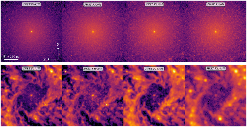
Figure 1: Overview of the nuclear region of NGC 628 in different bands. Each panel gives the central $$20\text{\,}\arcsec$\times$20\text{\,}\arcsec$$ (approximately $$950\text{\,}\mathrm{pc}$\times$950\text{\,}\mathrm{pc}$$) of the galaxy, centered on the nuclear star cluster. North is up and East is to the left. Color correlates with intensity. The first row gives three color-images using HST and JWST bands, highlighting star-formation by using the continuum-subtracted HST ACS F658N (H$\alpha$) filter. Dust lanes, where star formation occurs, are clearly visible in the first and third panel, while only stellar emission is shown in the second panel. The squared box of side length $5.5\text{\,}\arcsec$ in the third panel shows the region we considered for the fit of the NSC. The second row highlights other available data sets, namely the AstroSat ultraviolet emission, MUSE H$\alpha$, and ALMA CO. The first two panels trace again star formation whereas the third panel shows the location of the molecular gas. Note the absence of star formation and gas in the immediate vicinity of the nuclear star cluster, which is marked with a white cross. The third and fourth rows show the HST data, increasing in wavelength. Star forming regions, identified in the HST WFC3 F275W, become hidden behind dust filaments in other bands. The sixth panel, showing the HST ACS F814W data, mainly shows stellar emission. We show the newly obtained JWST NIRCam (fifth) and MIRI (sixth) in the last two rows, again in increasing wavelength from the near-infrared to the mid-infrared. The NIRCam data highlights the stellar emission while the MIRI data shows both stellar and dust emission. As for the molecular gas (ALMA CO, second row), a central cavity exists and dust is present in the spiral arms of NGC 628.

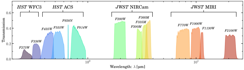
Figure 2: Transmission of the HST and JWST bands used in this work.

2 Data

Our analysis is based on archival HST ACS & WFC3 taken from the Hubble Legacy Archive and recently obtained JWST NIRCam & MIRI imaging data (project ID 02107, PI J. Lee; see Lee et al., in prep., this issue). A brief overview of the available data is given in Table 1 and Figure 2. In the next three subsections we briefly describe the data processing for each instrument, followed by the generation of point spread functions.

Table 1: Data used in this work.

Instrument	Channel	Filter	PropID	$t_{\mathrm{exp}}$	pixel scale
				[$\mathrm{s}$]	[$\mathrm{arcsec}\text{\,}{\mathrm{pixel}}^{-1}$]
HST	WFC3	F275W	13364	$4962.00$	$0.040$
HST	WFC3	F336W	13364	$4962.00$	$0.040$
HST	ACS	F435W	10402	$2716.00$	$0.050$
HST	ACS	F555W	10402	$1716.00$	$0.050$
HST	ACS	F658N	10402	$2844.00$	$0.050$
HST	ACS	F814W	10402	$1844.00$	$0.050$
JWST	NIRCam	F200W	02107	$9620.16$	$0.031$
JWST	NIRCam	F300M	02107	$773.048$	$0.063$
JWST	NIRCam	F335M	02107	$773.048$	$0.063$
JWST	NIRCam	F360M	02107	$858.944$	$0.063$
JWST	MIRI	F770W	02107	$266.40$	$0.110$
JWST	MIRI	F1000W	02107	$366.30$	$0.110$
JWST	MIRI	F1130W	02107	$932.412$	$0.110$
JWST	MIRI	F2100W	02107	$965.712$	$0.110$

2.1 Hubble Space Telescope

We obtain all available flat-fielded single exposures from the HLA to combine them into a single master frame. As a first step, the world coordinate systems of the ACS & WFC3 received updates using the latest reference files. These updated files were fed to AstroDrizzle (Fruchter et al., 2010; Gonzaga et al., 2012, see also Fruchter & Hook, 1997 for the drizzle algorithm), which combines them into a master science product given user-specified settings. As tested and justified in other work (Hoyer et al., 2022), we chose a pixel fraction of $0.75$ but keep the pixel scale at their original resolutions (see Table 1). No additional sky subtraction was performed as we account for background flux from the galaxy with a Sérsic profile (Sérsic, 1968) and a plane offset.

2.2 James Webb Space Telescope

As part of the “Physics at High Angular resolution in Nearby GalaxieS” (PHANGS) JWST cycle 1 treasury program, NGC 628 was observed in various NIRCam and MIRI bands on July 17, 2022 (see Table 1, and also Lee et al., in prep., this issue). Data reduction and co-addition were carried out using a custom data reduction pipeline, which among other things, improves the astrometric solutions and zero point offsets compared to the publicly available data products. More specifically, the world coordinate system (WCS) was updated to match the one from the HST and Gaia, and overall background level were calibrated against e.g. IRAC4 $8\text{\,}\mathrm{\SIUnitSymbolMicro m}$ and WISE3 $12\text{\,}\mathrm{\SIUnitSymbolMicro m}$ fluxes (Leroy et al., in prep., this issue). More detail of the customized version of the data reduction pipeline will be presented in Lee et al., in prep. (this issue).

2.3 Point spread functions

For all bands, we used artificially generated point spread functions (PSFs) instead of determining them from non-saturated stars in the images. The main reason for this choice was that no star is unaffected by dust and falls close to the location of the NSC (see Figure 1). Especially the latter condition is important for HST data as the PSF is known to vary significantly across the whole chip.

Following the approach by Hoyer et al. (2022), PSFs were generated using TinyTim (Krist, 1993, 1995) for HST bands. To minimize systematic differences in data processing, we did not directly use the resulting PSF from TinyTim for deriving the structural properties. Instead, we copied all input science frames and set their first header extension (science data) to zero. We then generated PSFs at the location of the NSC on each individual exposure and placed them into the previously normalized frames, taking into account the orientation of the original science images. Afterwards, we repeated the AstroDrizzle processing for the normalized frames in the same way as for the science data. The final PSF was extracted from the output of AstroDrizzle. In comparison to a PSF from TinyTim, the core of the extracted PSF is slightly more extended due to the drizzling process. Taking this effect into account is important for deriving accurate effective radii, as detailed in Hoyer et al. (2022).

Generation of PSFs for JWST bands was performed with WebbPSF (Perrin et al., 2012, 2014). To generate a star at the location of the NSC, we first generated a grid of 36 PSFs for the detector elements where the position of the NSC falls upon. The PSF for the position of the NSC was evaluated based on interpolation of generated PSFs using WebbPSF. This step is crucial as the PSF of JWST varies in both the spatial and temporal dimension (Nardiello et al., 2022). By default, and in agreement with our choice for the TinyTim-based PSFs, we chose a G2V star as the stellar template. As explored in Hoyer et al. (2022), the choice of stellar type plays little to no role on the fit results for HST data and we assume the same for JWST data.

3 Image fitting

3.1 Approach and model function

Focusing on the center of NGC 628, we extracted a square region of side length $5.5\text{\,}\mathrm{\SIUnitSymbolArcsecond}$ (equivalent to $\sim$260\text{\,}\mathrm{pc}$$) centered on the NSC to avoid the more dust- and gas-rich spiral structure, as shown in the first row, right panel of Figure 1. Previous investigations used various model functions to describe the light distribution of NSCs, including King profiles (see King, 1962 for the original definition; e.g. Matthews et al., 1999; Seth et al., 2006; Georgiev et al., 2009b; Georgiev & Böker, 2014), Gaussian profiles (e.g. Carollo et al., 1997, 2002; Barth et al., 2009; den Brok et al., 2014), Nuker profiles (see Lauer et al., 2005 for a definition, e.g. Carollo & Stiavelli, 1998; Böker et al., 1999, 2002; Butler & Martínez-Delgado, 2005), Sérsic profiles (e.g. Côté et al., 2006; Baldassare et al., 2014; Carson et al., 2015; Spengler et al., 2017; Pechetti et al., 2020), or point sources (e.g. Ferrarese et al., 2020; Poulain et al., 2021; Zanatta et al., 2021; Carlsten et al., 2022). Here we use the Sérsic profile of the form

$$I(r)=I_{\mathrm{eff}}\,\exp\bigg{\{}-b_{n}\,\bigg{[}\bigg{(}\frac{r}{r_{\mathrm{eff}}}\bigg{)}^{1/n}-1\bigg{]}\bigg{\}}\;,$$ (1)

where $r$ is the radius, $r_{\mathrm{eff}}$ the half-light or effective radius, $I_{\mathrm{eff}}$ the intensity at $r_{\mathrm{eff}}$, and $n$ the Sérsic index. The parameter $b_{n}$ solves the equation $\Gamma(2n)=2\gamma(2n,\,b_{n})$ where $\gamma(a,x)$ is the incomplete and $\Gamma(x)$ the complete Gamma function. For $n\in($0.5$,\,$10$)$, $b_{n}=$1.9992$n-$0.3271$$ is a good approximation (Capaccioli, 1989, but see also Graham & Driver, 2005 for a general overview).

The background flux from the host galaxy and the sky was modeled with another Sérsic profile and a plane offset. From our fits (see below), we found that in all bands $I_{\mathrm{eff}}^{\mathrm{gal}}\ll I_{\mathrm{eff}}^{\mathrm{nsc}}$, $r_{\mathrm{eff}}^{\mathrm{gal}}\gg r_{\mathrm{eff}}^{\mathrm{nsc}}$, and $n^{\mathrm{gal}}\lesssim 1$, such that the profile of the host galaxy becomes flat in the very center, thus justifying the choice of models. As we describe in Appendix A, two Sérsic profiles describe the NSC worse than a single profile.

To fit the data, we convolved the profiles with the previously generated synthetic PSF at the position of the NSC (see Section 2.3). The fit itself was performed with Imfit (Erwin, 2015), a specialized program to fit astronomical images. For the minimization technique, we chose the Differential Evolution solver with Latin hypercube sampling. In comparison with other available options, the solver does not rely on initial parameter values but randomly selects parameter values between user-specified boundaries (see Storn & Price, 1997, for details). We list the boundaries for the parameters of the Sérsic profile used for the NSC in Table 2. By default, Imfit evaluates the goodness of the fit with standard $\chi^{2}$ statistics.

Unless specified, Imfit assumes Poissonian statistics of the input data to generate a noise map. We take this approach for all but the JWST MIRI data where noise maps were generated by the previously mentioned custom data calibration pipeline. The noise maps for the MIRI bands were determined from uncertainties of the input data, the read noise and the flat fields, weighted by the fractional contribution to each pixel. As a result, compared to the standard noise map generated by Imfit, the MIRI noise maps give lower values for the nucleus itself, but higher values for the faint emission by the background galaxy.

In Figures 3 and 4 we show the data, best-fit two-component models, and the residuals for the HST ACS & WFC3, JWST NIRCam, and MIRI data, respectively. For the JWST MIRI F2100W all attempts failed to find a stable fit. Instead, to get an estimate for the apparent magnitude, we fit a Sérsic profile excluding PSF convolution.

Table 2: Sérsic parameters and their boundary values used to fit the data with Imfit. The same values are used for all HST and JWST bands.

Parameter	Boundary	Unit	Description
$x_{0}$	$[$45$,\,$55$]$	$\mathrm{pixel}$	NSC position
$y_{0}$	$[$45$,\,$55$]$	$\mathrm{pixel}$	NSC position
PA	$[$-359.99$,\,$359.99$]$	$\deg$	Position angle
$\epsilon$	$[$0.00$,\,$0.99$]$	–	Ellipticity
$n$	$[$0.00$,\,$5.00$]$	–	Sérsic index
$r_{\mathrm{eff}}$	$[$0.00$,\,$10.00$]$	$\mathrm{pixel}$	Effective radius
$I_{\mathrm{eff}}$	$[$0.00$,\,I_{\mathrm{max}}]$	counts	Intensity at $r_{\mathrm{eff}}$

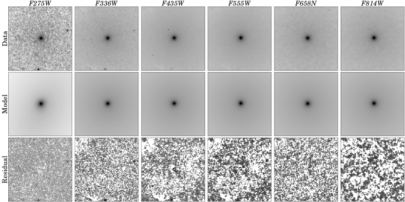
Figure 3: Overview of the central $$5.5\text{\,}\arcsec$\times$5.5\text{\,}\arcsec$$ ($$1\text{\,}\arcsec$\approx$47\text{\,}\mathrm{pc}$$) of NGC 628 in six different Hubble Space Telescope bands. North is up and East is left. Top row: Data products as used for fitting. Middle row: Model images of the best fit using one Sérsic profile for the nuclear star cluster, an additional Sérsic profile for the background, and a plane offset. Bottom row: Residual map, $\mathrm{Data}-\mathrm{Model}$. The gray scale of the maps are logarithmic and vary from $5\text{\times}{10}^{-3}$ to $5\text{\times}{10}^{2}$ times the mean of the residuals.

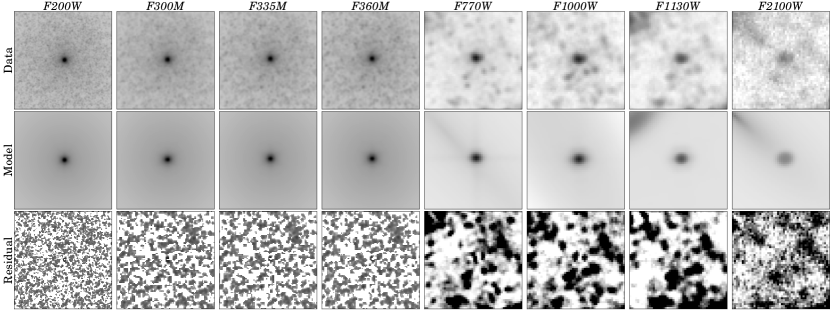
Figure 4: Overview of the same central region as in Figure 3 but for available JWST NIRCam and MIRI data. For the F2100W, no fit was possible including PSF convolution. The model shown here is a pure Sérsic profile without PSF convolution to determine the apparent magnitude of the source. For the MIRI data, we adjust the gray scales to $0.99$ and $1.01$ times the mean.

3.2 Uncertainties

We determined uncertainties by repeating the fit $500$ times using bootstrapping. During each iteration of bootstrapping, Imfit generates a new data array where indices of pixels are randomly sampled. During re-sampling, the pixel values of the input data as well as their location are not considered. The quoted best-fit parameters equal the median value of the parameter distribution and the uncertainties give the $$1$\sigma$ interval.

For some physical parameters, such as the determination of NSC mass (see Section 4.3) or the transformation of the effective radius to parsec, the bootstrapping uncertainties were propagated forward. Based on the assumption that the underlying probability distributions are Gaussians, we used the Gaussian error propagation.

The uncertainty of the zero point magnitudes for the HST bands is of the order $\mathcal{O}($10$^{$-3$})$ and can be neglected. However, recent analyses of early JWST data revealed that there exist issues with the flux calibration. As detailed below, these issues persist and remain significant

For the JWST NIRCam data, the uncertainty on the flux calibration can be as high as $0.2\text{\,}\mathrm{mag}$ (Boyer et al., 2022), depending on the band and detector. Most recent analyses in the community try to solve this issue by introducing multiplicative correction factors for the data. We corrected the determined fluxes by the mean multiplicative correction factor of G. Brammer and I. Labbe presented in Brammer (2022), $0.7845$. The correction factors are presented for the F090W, F115W, F150W, and F200W, that is, only the last band overlaps between the filter sets. To remain consistent between all four NIRCam bands, we did not change the value of the apparent magnitude, but determine the uncertainty from the multiplicative correction factor itself. The final uncertainty on the magnitude was then determined through Gaussian error propagation of this systematic uncertainty and the statistical uncertainty obtained from the fit. For the other three NIRCam bands, we assumed that the correction factor equals $0.8$, resulting in an uncertainty of $\sim$0.24\text{\,}\mathrm{mag}$$. As for the F200W, we combined this value with the statistical uncertainty from bootstrapping for the final uncertainty.

For the JWST MIRI data, the background level was, as described in Section 2.2, adjusted by comparing the F770W flux to the IRAC4 $8\text{\,}\mathrm{\SIUnitSymbolMicro m}$ and WISE3 $12\text{\,}\mathrm{\SIUnitSymbolMicro m}$ bands. The estimated uncertainty on its value is $\pm$0.1\text{\,}\mathrm{mag}$$ (Leroy et al., in prep., this issue).

As pointed out in Section 2.3, we did not check the influence the calibration and co-addition of the data have on the synthetic PSF generated by WebbPSF. Hoyer et al. (2022) found for the HST data that the co-addition of single exposures results in a slight broadening of the core of the PSF, introducing a systematic overestimation of the NSCs size. To repeat this experiment for the JWST data, we focused on the NIRCam F200W band and repeated the fit introducing an additional jitter in the form of a Gaussian function convolved with the synthetic PSF. In WebbPSF, we increased the jitter by factors of two and five and repeated the fits using the new PSFs. The result was that the structural parameters, as well as magnitude and color, remained well within the $$1$\sigma$ distribution of the original fits. Therefore, we conclude that our results are reliable given the presented uncertainties.

4 Analysis

4.1 Photometry

Integrating Equation 1 with an assumed ellipticity ($\epsilon$) yields the luminosity ($L$; photon count per energy band and time) as

$$L=$2$\pi\,($1$-\epsilon)\,I_{\mathrm{eff}}\,r_{\mathrm{eff}}^{$2$}\,\frac{n\mathrm{e}^{b_{n}}}{(b_{n})^{$2$n}}\,\Gamma($2$n)\;.$$ (2)

We use the equation

$$\mathrm{ZP}_{\mathrm{AB}}= $-2.5$\,\log_{10}\,(\,\mathrm{PHOTFLAM}\,)$$

$$$-5$\,\log_{10}\,(\,\mathrm{PHOTPLAM}\,)$$

$$$-2.408$\;,$$ (3)

to calculate the zero point magnitudes for HST ACS / WFC3 bands. The values of PHOTFLAM and PHOTPLAM are given in the header extensions of the fits files.

Pixel values in JWST data products have the unit $\mathrm{MJy}\text{\,}{\mathrm{sr}}^{-1}$, which we convert to $\mathrm{Jy}$ by using Equation 2 and the pixel-to-steradian conversion factor PIXAR_SR from the header extension. The zero point magnitude is then derived using

$$\mathrm{ZP}_{\mathrm{AB}}=$-2.5$\,\log_{10}\,(L)+$8.9$\;.$$ (4)

Foreground extinction is taken into account by using the re-calibrated version of the Schlegel et al. (1998) extinction maps (Schlafly & Finkbeiner, 2011) and assuming $R_{V}=$3.1$$ (Fitzpatrick, 1999). Due to the apparent lack of dust in the center of NGC 628, we do not attempt to correct for intrinsic extinction. For the HST bands, we derive $A(\lambda)\,/\,A(\mathrm{\textit{V}})$ with the model from O’Donnell (1994), which is based on Cardelli et al. (1989).

Figure 5 shows spectral flux densities as well as the extinction-corrected apparent magnitudes of the NSC in the AB-magnitude system. The NSC is faintest in the ultraviolet regime and becomes brighter towards the near-infrared. The brightest magnitude is reached at $2\text{\,}\mathrm{\SIUnitSymbolMicro m}$ after which the nucleus becomes fainter again.

To compare to the values by GB14, we transform our magnitudes from the AB- to the Vega-magnitude system using the approach outlined in Sirianni et al. (2005) and applied in Pechetti et al. (2020) for NSCs. We find $\mathrm{\textit{V}}_{0}=($17.85$\pm$0.04$)\,$\mathrm{mag}$$ and $\mathrm{\textit{I}}_{0}=($16.69$\pm$0.05$)\,$\mathrm{mag}$$. GB14 present $\mathrm{\textit{V}}_{0}=($17.88$\pm$0.01$)\,$\mathrm{mag}$$ and $\mathrm{\textit{I}}_{0}=($16.57$\pm$0.01$)\,$\mathrm{mag}$$. While the $V$-band magnitudes agree with each other, we find a significant difference in the I-band. The different magnitude is most likely related to the extracted structural parameters (cf. Section 4.4).

4.2 SED modeling

The combined HST and JWST data cover the ultraviolet to mid-infrared spectrum and enable the study of the spectral energy distribution (SED) in detail. To extract basic parameters describing the stellar population, we set up a model assuming a delayed star formation history, two commonly used different initial mass functions (Chabrier, 2003; Salpeter, 1955), and the Bruzual & Charlot (2003) single stellar population model.

The fits were executed using CIGALE, a Python code for modeling the SEDs of galaxies (see Boquien et al., 2019, and Burgarella et al., 2005; Noll et al., 2009; Yang et al., 2020, 2022), which has successfully been applied to star clusters (e.g. Fensch et al., 2019; Turner et al., 2021). The program allows to adjust various physical properties such as the age of the stellar populations or their metallicity. We test various parameter values, as detailed in Table 3, to find the best possible fit to the data, as evaluated by Bayesian statistics.

Table 3: Parameters values for the spectral energy distribution fits. The values remain unchanged between runs including and excluding the MIRI data.

Parameter	Unit	Values	Best-fit		Notes
			Incl. MIRI	Excl. MIRI
Star formation history
tau_main	[$\mathrm{Myr}$]	$1$, $10$, $100$, $1000$, $2000$, $3000$	$$500$\pm$500$$	$$220$^{+380}_{-220}$	e-folding time of the main stellar population
age_main	[$\mathrm{Gyr}$]	$3$, $4$, $5$, $6$, $7$, $8$, $9$, $10$, $11$, $12$, $13$	$$8$\pm$2$$	$$8$\pm$3$$	Age of the main stellar population
tau_burst	[$\mathrm{Myr}$]	$10$, $20$, $50$, $100$	$$57$\pm$33$$	$$57$\pm$33$$	Time of the late starburst
age_burst	[$\mathrm{Myr}$]	$10$, $20$, $50$, $100$	$$27$\pm$17$$	$$27$\pm$17$$	Age of the late burst
f_burst	–	$0.0$, $0.1$, $0.2$, $0.5$	$$0$\pm$0$$	$$0$\pm$0$$	Mass fraction of the late burst
Simple stellar population
imf	–	$0$, $1$	$1$	$1$	Initial mass function (Salpeter, 1955, Chabrier, 2003)
metallicity	–	$0.004$, $0.008$, $0.02$, $0.05$	$$0.027$\pm$0.013$$	$$0.012$\pm$0.006$$	Metallicity of the stellar population

The fit was performed twice, excluding the MIRI data in one run. We do this to test their influence to the fit result and disentangle emission from low-mass stars and dust. The addition of a dust emission model yielded worse fits, as evaluated by both the reduced $\chi^{2}$ and Bayesian statistics, which is why we do not include it in the presented results. We discuss this issue in more detail in Section 5.

For the fit including the MIRI data, we find that the mass-weighted age of the main stellar population is $($8$\pm$2$)\,$\mathrm{Gyr}$$ with a metallicity of $Z=$0.03$\pm$0.01$$, slightly more metal-rich than the Sun (Asplund et al., 2009). The e-folding time of the main stellar population is $($500$\pm$500$)\,$\mathrm{Myr}$$ and the mass fraction of the late burst is consistent with zero. The fit preferred a Chabrier (2003)-type initial mass function over a Salpeter (1955) one.

For the fit excluding the MIRI data, we find a mass-weighted age of the main stellar population of $($8$\pm$3$)\,$\mathrm{Gyr}$$ with a metallicity of $Z=$0.012$\pm$0.006$$. The e-folding time was determined to be $$220$_{$-220$}^{$380$}\,$\mathrm{Myr}$$ and the mass fraction of the late burst is comparable to zero. The fit again preferred a Chabrier (2003)-type initial mass function.

According to the reduced $\chi^{2}$ statistics, the fit excluding the MIRI data performed better than the one including them. The results of both fits are consistent with each other, indicating the presence of a $8\text{\,}\mathrm{Gyr}$ old stellar population with metallicity $Z\sim$0.02$$ and no presence of a young stellar population. We discuss the results obtained for the mass of the stellar population in the next section.

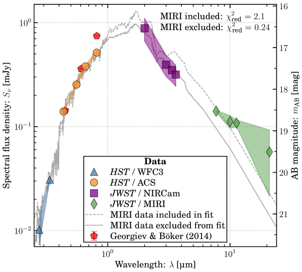
Figure 5: Spectral flux density ($S_{\nu}$, left axis) and AB magnitude ($m_{\mathrm{AB}}$, right axis) versus wavelength ($\lambda$). Different instruments are highlighted with marker symbols and colors. Red pentagons give the results by Georgiev & Böker (2014) in the Vega-magnitude system. Uncertainties are indicated with shaded areas. Two gray lines show the spectral energy distribution fits to the data including (dashed line) and excluding (solid line) the JWST MIRI data. The goodness of the fits is given by reduced $\chi^{2}$ values in the panel. For both fits, we use the Bruzual & Charlot (2003) stellar population model and a delayed star formation history. The fit prefers a Chabrier (2003) initial mass function over the prescription by Salpeter (1955). Both fits indicate the presence of a $8\text{\,}\mathrm{Gyr}$ old stellar population with metallicity $Z\sim 0.02$. No younger stellar population could be detected.

4.3 Stellar mass

We determine the stellar mass of the NSC in three different ways: (1) we use $\mathrm{\textit{B}}-\mathrm{\textit{V}}$ color and its mass-to-light scaling relations, (2) we combine the apparent magnitude in the F200W (roughly K-band) with a constant mass-to-light ratio ranging between $0.5$ and $0.6$ (in solar units), and (3) we extrapolate a stellar mass from SED fitting. The resulting mass estimates and the literature value from Georgiev et al. (2016) are presented in Table 4.

Following Hoyer et al. (2021), we use four different $\mathrm{\textit{B}}-\mathrm{\textit{V}}$ color relations and the V-band luminosity to obtain a stellar mass-to-light ratio. The original relations were published by Bell et al. (2003); Portinari et al. (2004); Zibetti et al. (2009); Into & Portinari (2013) but we adopt the revised parameters from McGaugh & Schombert (2014), which ensures consistency between the relations. An extended discussion and the assumptions made are detailed in Hoyer et al. (2021).

First, the HST ACS F435W and F555W magnitudes were converted to the Johnson-Cousin system (B- and V-band, respectively) using Equation $12$ and Table $22$ from Sirianni et al. (2005). Absolute magnitudes were derived using the distance estimate of the galaxy and the absolute magnitude of the Sun (Willmer, 2018).

After transforming the HST magnitudes to the Johnson-Cousin system and using magnitudes in the Vega-system, we find $\mathrm{\textit{B}}_{0}=($18.59$\pm$0.03$)\,$\mathrm{mag}$$ and $\mathrm{\textit{V}}_{0}=($17.86$\pm$0.04$)\,$\mathrm{mag}$$ with a color $(\mathrm{\textit{B}}-\mathrm{\textit{V}})_{0}=($0.73$\pm$0.05$)\,$\mathrm{mag}$$, which roughly matches the color of a G8V-type star ($\mathrm{\textit{B}}-\mathrm{\textit{V}}\sim 0.75$) and is consistent with the results from the SED fits. From the four scaling relations, we determine individual masses and combine them into one using the weighted average. The resulting mass estimate is $\log_{10}\,(M_{\star}^{\mathrm{nsc}}\,/\,$\mathrm{M_{\odot}}$)=$7.06$\pm$0.31$$. The uncertainty budget is dominated by the uncertainty assumed for the mass-to-light ratio, $0.3\text{\,}\mathrm{dex}$ (Roediger & Courteau, 2015).

An alternative approach is to use the magnitude in the K-band. McGaugh & Schombert (2014) found that a constant mass-to-light ratio of $\sim$0.6$$ can be used to estimate stellar masses as the near-infrared luminosity is only weakly dependent on color. While we do not directly have a K-band magnitude, we estimate the mass using the F200W band from JWST, centered on $2\text{\,}\mathrm{\SIUnitSymbolMicro m}$. The K-band overlaps with the F200W band such that we can use the mass estimate as a benchmark for the other mass estimates.

Using the same four references as for the approach using the $\mathrm{\textit{B}}-\mathrm{\textit{V}}$ color (Bell et al., 2003; Portinari et al., 2004; Zibetti et al., 2009; Into & Portinari, 2013) and their re-calibrated values from McGaugh & Schombert (2014), we find a stellar mass of $\log_{10}\,(M_{\star}^{\mathrm{nsc}}\,/\,$\mathrm{M_{\odot}}$)=$7.2$\pm$1.1$$. The uncertainty is much larger than for the mass determined from the $\mathrm{\textit{B}}-\mathrm{\textit{V}}$ relation due to the uncertainty on the zero point of the NIRCam data.

From the SED fitting in the previous section, the mass of the star cluster was determined as well. In the fit including the MIRI data, we find $\log_{10}\,(M_{\star,\,1}^{\mathrm{nsc}}\,/\,$\mathrm{M_{\odot}}$)=$7.17$\pm$0.10$$. In the fit excluding the MIRI data, we find $\log_{10}\,(M_{\star,\,2}^{\mathrm{nsc}}\,/\,$\mathrm{M_{\odot}}$)=$7.11$\pm$0.10$$. As stated above, no young stellar population was found.

The mass of the NSC was previously determined by Georgiev et al. (2016) based on the analysis of GB14. To obtain stellar masses, the authors use stellar population models from Bruzual & Charlot (2003) with solar metallicity and an initial mass function of the type presented in Kroupa (2001). The reported mass for the NSC of NGC 628 is $\log_{10}\,(M_{\star}^{\mathrm{nsc}}\,/\,$\mathrm{M_{\odot}}$)=$7.05$\pm$0.21$$, which agrees within the uncertainty with our mass estimates.

Overall, we find agreement between all approaches finding that the NSC has a stellar mass of $\sim${10}^{7}\text{\,}\mathrm{M_{\odot}}$$. In the following, we use the mass value $\log_{10}\,(M_{\star}^{\mathrm{nsc}}\,/\,$\mathrm{M_{\odot}}$)=$7.06$\pm$0.31$$.

Table 4: Determined nuclear star cluster mass as well as the literature value.

Method	Logarithmic stellar mass
	[$\mathrm{M_{\odot}}$]
$\mathrm{\textit{B}}-\mathrm{\textit{V}}$	$$7.06$\pm$0.31$$
K-band	$$7.2$\pm$1.1$$
SED (incl. MIRI)	$$7.17$\pm$0.10$$
SED (excl. MIRI)	$$7.11$\pm$0.10$$
Georgiev et al. (2016)	$$7.05$\pm$0.21$$

4.4 Structure

Figure 6 shows the effective radius, ellipticity, Sérsic index, and position angle versus wavelength (from Section 3). We also add the literature values by GB14.

In panel A, we show the effective radius versus wavelength. It remains roughly constant at $\sim$5\text{\,}\mathrm{pc}$$ in the ultraviolet and optical regime, but starts to slightly increase towards $\sim$6\text{\,}\mathrm{pc}$$ at $3.6\text{\,}\mathrm{\SIUnitSymbolMicro m}$. This trend continues into the mid-infrared where $r_{\mathrm{eff}}\sim$12\text{\,}\mathrm{pc}$$.

GB14 find different effective radii ranging from $\sim$2\text{\,}\mathrm{pc}$$ to $\sim$3.5\text{\,}\mathrm{pc}$$. They modeled the NSC light distribution by convolving a TinyTim-generated PSF with King profiles of different concentration parameters (ratio of the tidal to core radius: $5$, $15$, $30$, and $100$). Using ISHAPE (Larsen, 1999), they fit the data and used the best-fit model, according to $\chi^{2}$ residuals to derive the effective radius of the cluster. In their fits, a concentration parameter of $100$ gave the best results. The final value for the effective radius was obtained by taking the geometric mean of the full-width-half-maximum along the semi-minor and major axes and using a transformation factor from ISHAPE’s manual.

In the ultraviolet and optical regime, the ellipticity is $\sim$0.05$$ (panel B in Figure 6). It remains in this range at $2\text{\,}\mathrm{\SIUnitSymbolMicro m}$ and $3\text{\,}\mathrm{\SIUnitSymbolMicro m}$, but starts to increase to $\sim$0.1$$ at $3.6\text{\,}\mathrm{\SIUnitSymbolMicro m}$. At even longer wavelengths, the ellipticity increases to $\sim$0.4$$ and is significantly different from the other wavelength regimes. Our measurements in the optical are consistent with the ones presented by GB14, but are smaller than the typical ellipticity for other NSCs in the same mass range ($\epsilon\gtrsim$0.1$$, e.g. Seth et al., 2006; Carson et al., 2015; Spengler et al., 2017; Hoyer et al., 2022).

The Sérsic index (panel C) appears to vary with wavelength. In the ultraviolet and optical regime, we find $n\sim$3$$, but in the near-infrared the value drops to $\sim$2$$. At the longest wavelengths, the value drops to $\sim$1.5$$, but is also consistent with an exponential profile ($n=$1$$). GB14 used a King profile to approximate the light distribution and no comparison can be made.

The position angle of the NSC (panel D) starts at $\sim$130\text{\,}\mathrm{\SIUnitSymbolDegree}$$ in the ultraviolet regime. Starting in the optical regime, the position angle drops to $\sim$100\text{\,}\mathrm{\SIUnitSymbolDegree}$$ and shows a mild anti-correlation with wavelength, dropping further to $\sim$90\text{\,}\mathrm{\SIUnitSymbolDegree}$$ in the mid-infrared. Only the data point from the HST WFPC2 PC F606W band by GB14 is consistent with our results. The other two data points are significantly elevated to $\sim$135\text{\,}\mathrm{\SIUnitSymbolDegree}$$ and $\sim$160\text{\,}\mathrm{\SIUnitSymbolDegree}$$.

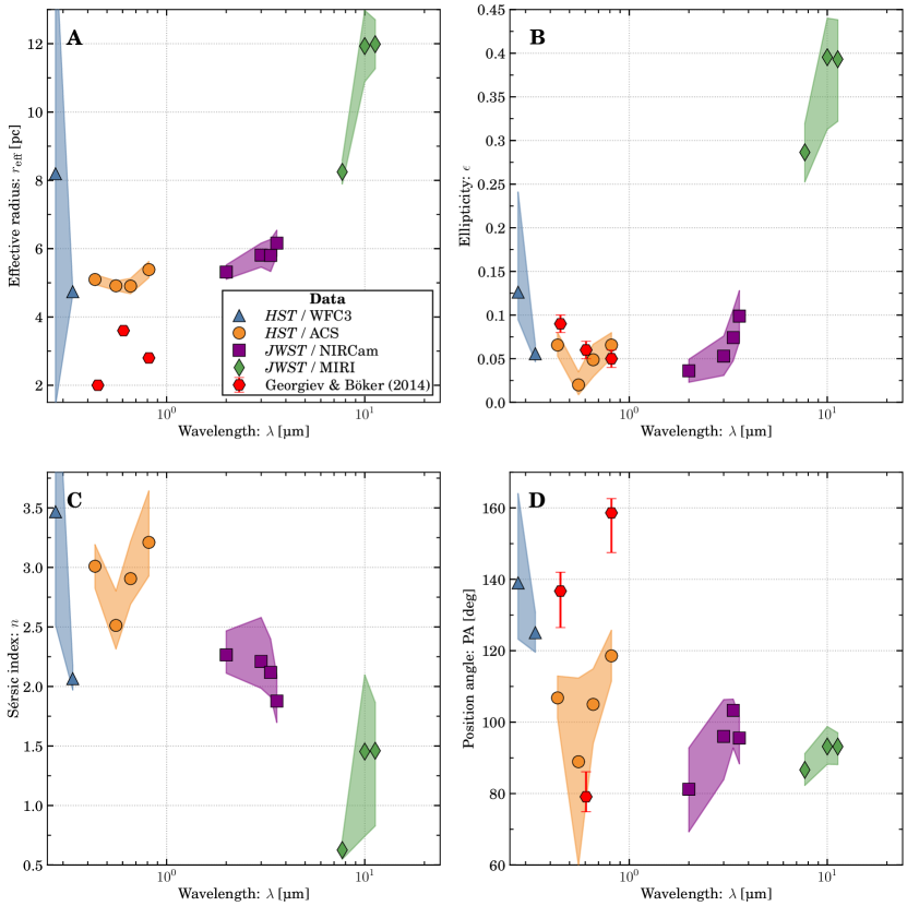
Figure 6: Structural properties of the nucleus of NGC 628: effective radius (panel A), ellipticity (panel B), Sérsic index (panel C), and position angle (panel D) versus wavelength. Marker symbols and colors highlight different instruments. Uncertainties are shown with shaded areas. Red pentagons show literature values from Georgiev & Böker (2014).

4.5 Astrometric offset

From the previous section it is apparent that the nucleus shows an evolution with wavelength, especially towards the mid-infrared regime. Here we investigate the variability of the central position of the emission in different bands.

In Figure 7 we show the emission in the JWST MIRI F2100W band (gray scale and white contour lines) and overlay the emission from the HST WFC3 F275W band. The WCS of each band were taken from the bands header files. We find that there exists an offset between the centers of the emission, separated by $\sim$0.2\text{\,}\arcsec$$, which approximates to $\sim$9.5\text{\,}\mathrm{pc}$$ at the distance to the galaxy.

To test whether the offset persists in other bands, we perform the following experiment: we determine the angular coordinates for other bands based on the central position of the Sérsic profile fit to the light distribution. Figure 8 presents the resulting angular separation using the HST WFC3 F275W band as reference. We find that the angular separation is of the order of $\lesssim$0.1\text{\,}\mathrm{\SIUnitSymbolArcsecond}$$ ($\lesssim$5\text{\,}\mathrm{pc}$$) in the optical, which is comparable to the effective radius of the cluster. In the infrared the separation drops to $\lesssim$0.06\text{\,}\mathrm{\SIUnitSymbolArcsecond}$$ but increases up to $0.21\text{\,}\mathrm{\SIUnitSymbolArcsecond}$ in the mid-infrared regime.

Depending on the band used as reference, the angular separation can become insignificant. For example, while using the F200W as reference, the offsets in the MIRI bands are still significant, whereas they become insignificant, except for the F1000W, when using the F335M as reference. This behavior could point towards issues with the calibration of the WCS’: while we calibrated all HST data with the most recent WCS solutions from MAST, no reliable solutions exist so far for the JWST data. The PHANGS-internal versions of the data were calibrated in the following way: The NIRCam data was calibrated using HST and Gaia astrometric solutions using asymptotic giant branch stars. Furthermore, the direction of the separation is the same in the MIRI bands, towards the North-West (as seen in Figure 7).

Compared to the HST data, the NIRCam calibration should yield “accurate” astrometric values (see below). The MIRI data are astrometrically aligned to the F335M image by cross-correlating the images and solving for relative offsets. However, due to variations in the polycyclic aromatic hydrocarbons emission structure between different bands and the lack of point-like emission in the MIRI bands, the astrometric calibration is less certain.

To further quantify the offsets and benchmark the values, we compute the angular separation of (a) a star outside the central cavity, (b) multiple stars less than $1\text{\,}\arcsec$ South of the NSC within the cavity, and (c) a GC about $10\text{\,}\arcsec$ South-West from the NSC. The star outside the cavity has Gaia EDR3 designation 2589386446469602688, is non-saturated in all but the HST ACS F435W, F555W, and F814W bands and lies about $60\text{\,}\mathrm{\SIUnitSymbolArcsecond}$ South-East of the NSC. For the star outside the cavity and the GC, we fit the light distribution with a two-dimensional Gaussian function, which yields the position of the center of the sources, which we deem accurate within $0.5\text{\,}\mathrm{pixel}$. For the other stars close to the NSC, we extract the position manually.

In Figure 8 we show the offset of the star outside the cavity and the GC in addition to the offsets for the NSC. If we use the HST WFC3 F275W data as reference, the offsets are significant in both the NIRCam and MIRI data. The same result is found if we use the F200W as reference. However, the offsets become insignificant in all except two bands (F200W & F1000W) if we use the F335M data as reference. With the currently available WCS calibrations, while there are hints of an astrometric offset, we cannot conclude whether they are significant.

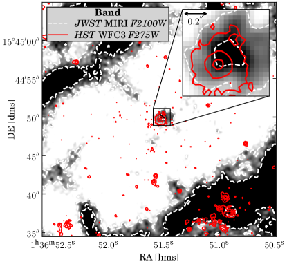
Figure 7: Main panel: Central $$5.5\text{\,}\mathrm{\SIUnitSymbolArcsecond}$\times$5.5\text{\,}\mathrm{\SIUnitSymbolArcsecond}$$ of NGC 628 in the JWST MIRI F2100W. A darker shade and white contours show high flux in the F2100W. Red contours highlight the HST WFC3 F275W emission. Both maps are matched based on the most up-to-date world coordinate solutions. Inset panel: Zoom into the nucleus of NGC 628. The white and red contours highlight again the emission in the F2100W and F275W, respectively. The offset between the centers of the contours measures approximately $0.2\text{\,}\mathrm{\SIUnitSymbolArcsecond}$.

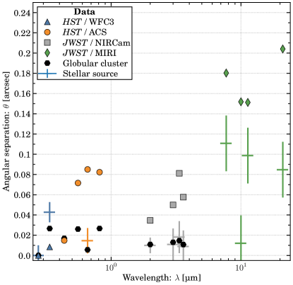
Figure 8: Angular separation ($\theta$) versus wavelength ($\lambda$) of the nuclear star cluster position with respect to the HST WFC3 F275W. Different instruments are highlighted with different marker symbols and colors. Crosses show the angular separation of a star with Gaia EDR3 designation 2589386446469602688. The vertical length of the cross give $0.5\text{\,}\mathrm{pixel}$, which we assume as an upper limit on extracting the position of the star. Data points above the crosses indicate that either the world coordinate system is offset, or the center of the nucleus is offset compared to the HST WFC3 F275W. In some bands (for example the HST ACS F814W), the star is saturated and no central position could be determined. The separations for a globular cluster, located $\sim$10\text{\,}\arcsec$$ South-West of the nucleus is shown with black hexagons. The offsets agree with the offsets of the star in the NIRCam data.

5 Discussion

One of the most striking features of the JWST observations of the center of NGC 628 is that the prominent NSC sits in a nuclear stellar component that is devoid of gas and dust. It appears that both gas and dust have been evacuated from the central cavity. The mechanism that created this cavity is not obvious. There are no young stars that could have blown out the gas recently. Alternatively, the central cavity could have been created by consumption of the gas in the last star formation event, and the re-supply of gas is hindered by a potential bar resonance, in case a bar is (or previously was) present.

5.1 Nuclear star cluster properties

We show the mass ratio (NSC mass divided by host galaxy mass) in the left panel of Figure 9 where the NSC of NGC 628 is highlighted with a blue cross. Data from the Local Volume (a field environment with distance $\lesssim$11\text{\,}\mathrm{Mpc}$$; Seth et al., 2006; Georgiev et al., 2009a; Graham & Spitler, 2009; Baldassare et al., 2014; Schödel et al., 2014a; Calzetti et al., 2015; Carson et al., 2015; Crnojević et al., 2016; Nguyen et al., 2017; Baumgardt & Hilker, 2018; Nguyen et al., 2018; Bellazzini et al., 2020; Pechetti et al., 2020) are added for comparison. Dwarfs around massive field galaxies and Virgo cluster members are taken from Carlsten et al. (2022) and Sánchez-Janssen et al. (2019a), respectively. Data for other massive late-type galaxies in the field are taken from GB14. The NSC of NGC 628 follows the overall trend in that the NSC mass becomes insignificant compared to the host galaxy. However, other late-types of the same host galaxy mass typically host more massive NSCs.

The effective radius of the NSC in NGC 628 also compares well to those of other NSCs in late-type galaxies (in the F814W band; middle panel in Figure 9). Finally, the ellipticity in the F814W band is smaller than the typical value in other late-types (right panel). This figure shows there exists no apparent correlation with the inclination of the host.

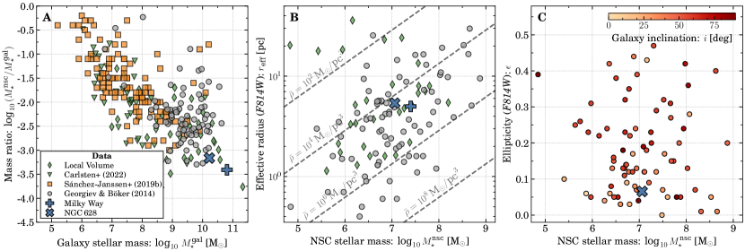
Figure 9: Left panel: Mass ratio of nuclear star cluster (NSC) and host galaxy stellar mass ($M_{\star}^{\mathrm{nsc}}/M_{\star}^{\mathrm{gal}}$) versus galaxy stellar mass. The NSC of NGC 628 is highlighted with a blue cross. Other data sets from the Local Volume (a field environment with a distance $\lesssim$11\text{\,}\mathrm{Mpc}$$; green diamonds; Seth et al., 2006; Georgiev et al., 2009a; Graham & Spitler, 2009; Baldassare et al., 2014; Schödel et al., 2014a; Calzetti et al., 2015; Carson et al., 2015; Crnojević et al., 2016; Nguyen et al., 2017; Baumgardt & Hilker, 2018; Nguyen et al., 2018; Bellazzini et al., 2020; Pechetti et al., 2020), the Virgo galaxy cluster (orange squares; Sánchez-Janssen et al., 2019a), dwarfs around massive field galaxies (green triangles; Carlsten et al., 2022), and massive field galaxies (gray circles; Georgiev & Böker, 2014) show the general distribution of NSCs. The Milky Way NSC is highlighted with a blue plus-sign. In comparison to other massive field late-type galaxies, the NSC of NGC 628 appears under-massive. Middle panel: Effective radius ($r_{\mathrm{eff}}$) in the F814W versus NSC stellar mass. The markers and colors of the data points are the same as in the left panel. Dashed lines give the mean density of clusters. Right panel: Ellipticity ($\epsilon$) versus NSC stellar mass. We show the data by Georgiev & Böker (2014) and color-code them by the host galaxy inclination. There exists no apparent correlation between ellipticity, mass, or inclination. For NGC 628, the inclination has a value of $i\sim$8.9\text{\,}\mathrm{\SIUnitSymbolDegree}$$ (Lang et al., 2020).

Since the mass of the NSC is smaller than most other masses of such a cluster at $M_{\star}^{\mathrm{gal}}\sim${10}^{10}\text{\,}\mathrm{M_{\odot}}$$ and assuming that stars formed in-situ should dominate the mass budget, we speculate that the NSC had a quiet evolution and that, compared to other NSCs, only little mass formed in-situ over the last few $\mathrm{Gyr}$. This speculation is corroborated by our results in Sections 4.1, 4.2, and 4.4: the effective radius shows no wavelength dependence from the ultraviolet to the near-infrared regime, staying roughly constant at $5\text{\,}\mathrm{pc}$. The color of the NSC was determined to be $\mathrm{\textit{B}}-\mathrm{\textit{V}}=($0.73$\pm$0.05$)\,$\mathrm{mag}$$, which compares to a star of G8V-class. Finally, the resulting best-fit SED model indicate that all stellar mass is assembled in an “old” stellar population, with the mass of the “young” stellar population being consistent with zero. As indicated by the fit, “old” refers to an age of $8\text{\,}\mathrm{Gyr}$. If true, this could also mean that the cavity has existed for a few $\mathrm{Gyr}$ and that any massive black hole in the center of NGC 628 did not grow significantly via gas accretion over the same time period. So far, no reliable black hole mass measurement is available (see also Section 5.3.1 below).

The SED fit also indicates that the metallicity of the NSC is $Z\sim$0.02$$, which is comparable to NSCs in similar mass galaxies (Koleva et al., 2009; Paudel et al., 2011; Spengler et al., 2017; Kacharov et al., 2018; Neumayer et al., 2020), and also the Milky Way NSC (Do et al., 2015; Feldmeier-Krause et al., 2017a). In combination with the age estimate of the stellar population, this reveals that the NSC formed in a dense environment where rapid enrichment took place. Such conditions could take place either during the formation of the galaxy itself or during a past merger event.

As mentioned above, while in-situ star formation is expected to contribute a significant mass fraction to the NSC, as measured in other galaxies, our results indicate that no in-situ star formation occurred over the last few $\mathrm{Gyr}$. This means that, since the formation of the NSC, either no or very little amount of gas fell towards the center or that star formation was inefficient. One possibility is that the shape of the gravitational potential limits the amount of inflow. Indeed, it is well known that in a viscous accretion disk, the amount of inward mass transport depends on the amount of shear (e.g. Shakura & Sunyaev, 1973; Lynden-Bell & Pringle, 1974). One way to limit the inflow of gas is to have a low shear, meaning that the rotation curve is close to solid body rotation (e.g. Lesch et al., 1990; Krumholz & Kruijssen, 2015). Note, however, that it is still unclear what mechanism drives the ISM turbulence responsible for creating the required viscosity (e.g. Klessen & Glover, 2016; Sormani & Li, 2020). Alternatively, it could be that the in-flow is irregular and triggered by mergers or interactions with satellite galaxies (e.g. Storchi-Bergmann & Schnorr-Müller, 2019). Multiple dwarfs are known to reside around NGC 628 (Davis et al., 2021) and numerous accretion events occurred in the galaxy’s history (Kamphuis & Briggs, 1992).

5.2 Comparison with the Milky Way

The obtained NSC size using near-infrared data seems to be very similar to the Milky Way’s (MWNSC) with an effective radius of $\sim$5\text{\,}\mathrm{pc}$$ (e.g. Fritz et al., 2016; Gallego-Cano et al., 2020). However, the MWNSC also presents a similar size when analyzed with Spitzer/IRAC mid-infrared data (Schödel et al., 2014b; Gallego-Cano et al., 2020), which is in contrast to the significantly larger effective radius we obtained for the NSC of NGC 628 from MIRI mid-infrared data. In addition, the mass estimates compare, with the MWNSC having a mass of $\sim$2\text{\times}{10}^{7}\text{\,}\mathrm{M_{\odot}}$$ (Launhardt et al., 2002; Schödel et al., 2014a; Feldmeier-Krause et al., 2017b).

The predominantly old ($\sim$8\text{\,}\mathrm{Gyr}$$) and metal-rich ($Z\sim$0.02$$) population detected in NGC 628’s NSC is also in agreement with the results obtained for the MWNSC (e.g. Feldmeier-Krause et al., 2017a; Schödel et al., 2020; Nogueras-Lara, 2022), though recent work suggested a younger age for the MWNSC of $\sim$5\text{\,}\mathrm{Gyr}$$ (Chen et al., 2022). However, the MWNSC also shows recent star formation activity, about $6\text{\,}\mathrm{Myr}$ ago (Paumard et al., 2006), which is not present in NGC 628’s NSC, according to the best-fit SED model.

Overall, we find that little to no star formation occurred in the last few $\mathrm{Gyr}$ in NGC 628’s center. This results in an under-massive NSC, compared to other similar-mass late-type galaxies, a likely under-massive central black hole, if present, and that the central cavity spanning approximately $$200\text{\,}\mathrm{pc}$\times$400\text{\,}\mathrm{pc}$$ existed for a similar period.

5.3 Nature of the emission in the mid-infrared

While an old ($8\text{\,}\mathrm{Gyr}$) population with metallicity $Z\sim$0.02$$ accounts for the emission in the ultraviolet to near-infrared regime, we found an excess of emission in the mid-infrared bands (cf. Figure 5), which cannot be explained by that same population. In addition, the effective radius and ellipticity do not change with wavelength until the mid-infrared regime, the Sérsic index shows a weak wavelength dependence, and the position angle does not change significantly between the near- and mid-infrared (cf. Figure 6). We speculate about the nature of the emission in the following sections.

5.3.1 Active galactic nucleus contribution

One possibility is that the emission in the mid-infrared bands is caused by an active galactic nucleus (AGN) once X-ray photons are absorbed by dust, which re-emits the radiation at longer wavelengths.

The presence of a massive black hole in NGC 628 is still disputed: Dong & De Robertis (2006) use the black hole mass versus bulge $\mathrm{\textit{K}}_{\mathrm{\textit{S}}}$-magnitude relation to find $\log_{10}\,(M_{\mathrm{BH}}\,/\,$\mathrm{M_{\odot}}$)\sim$6.7$$ but such a relation assumes that the bulge did not significantly grow through secular processes, which is believed to be the case for NGC 628. She et al. (2017) found an X-ray excess in the galaxy’s center, which they attribute to the presence of an AGN with a black hole mass of $\log_{10}\,(M_{\mathrm{BH}}\,/\,$\mathrm{M_{\odot}}$)\sim$6.0$$. The X-ray luminosity was determined to be $\log_{10}\,(L_{2\textrm{-}$10\text{\,}\mathrm{keV}$}\,/\,$\mathrm{W}$)=$31.15$^{+$0.32$}_{$-0.19$}$, as determined through the hardness ratios of soft-, medium-, and hard X-ray bands.

We determine the spectral flux density of the emission in the mid-infrared by using this luminosity and the scaling relation by Asmus et al. (2015), which connects the X-ray luminosity of an AGN to the mid-infrared luminosity at $12\text{\,}\mathrm{\SIUnitSymbolMicro m}$. The result is $S_{\nu}^{\mathrm{BH}}\sim$1.9\text{\times}{10}^{-4}\text{\,}\mathrm{mJy}$$. We compare this value to the difference between the observed emission and the model flux excluding the MIRI data in the $11.3\text{\,}\mathrm{\SIUnitSymbolMicro m}$ band. The difference equals $\Delta S_{\nu}^{$11.3\text{\,}\mathrm{\SIUnitSymbolMicro m}$}\sim$0.06\text{\,}\mathrm{mJy}$$, far exceeding the expected flux density of an AGN. Therefore, while the X-ray excess measured by She et al. (2017) originating from a possible AGN could contribute to the mid-infrared emission, it cannot fully explain it by itself. Furthermore, little to no dust is present in the NSC, making this scenario unlikely.

5.3.2 Infalling star cluster

A possible scenario, which could perhaps explain the offset in Figure 7, if real, is that we see the NSC and an in-falling star cluster, where the latter could be in a late stage of tidal disruption by the more massive NSC. Such a scenario for the build-up of NSCs has been proposed for a few decades (Tremaine et al., 1975) and is sometimes referred to as the “dry-merger” scenario (e.g. Arca Sedda & Gualandris, 2018) with ample observational and theoretical evidence in both the Galactic but also extragalactic NSCs (e.g. Antonini, 2013, 2014; Arca-Sedda & Capuzzo-Dolcetta, 2017; Fahrion et al., 2020; Feldmeier-Krause et al., 2020).

The proposed scenario could occur as follows: the star cluster would form outside the nuclear region and spiral inwards. During this time, the star cluster can be considered self-gravitating, which implies that it evolved predominantly due to its internal collisional dynamics. During the infall of the cluster, it will experience gravothermal-gravogyro contraction and core-collapse (e.g. Kamlah et al., 2022), mass segregate, and form a subsystem of black holes in its center, or even an intermediate-mass black hole, if the star cluster is massive enough. The most-massive stars accumulate in the star cluster’s center and lower-mass stars occupy the halo of the star cluster. Some of these low-mass stars will be stripped by the tidal field of the surrounding field or may be ejected through dynamical interactions, while the star cluster approaches the NSC. Some of the stripped or ejected stars might be visible as asymptotic giant branch (AGB) stars (see also Section 5.3.3) with their strong, dust-driven stellar winds (see Decin, 2021, and sources therein) in the near- to mid-infrared bands as single sources scattered around the NSC (see Figure 4).

From $N$-body simulations by Arca Sedda & Gualandris (2018), modeling the MWNSC and an infalling star cluster, we know what the infall, merger, and merger product phases look like in spatial coordinates (Figure 2 in Arca Sedda & Gualandris, 2018 and Figure 1 in Arca Sedda et al., 2020). If the infalling star cluster has already crossed the effective radius of the NSC, after which the star cluster becomes entirely tidally disrupted and cannot be considered a self-gravitating system anymore (Arca Sedda et al., 2020), the simulation snapshots could explain the potential astrometric offset. The star cluster’s core would eventually fall into the core of the NSC and the remaining halo stars would tidally disperse. Among these would be AGB stars that may partly be responsible for the astrometric offset shown in Figure 7 and contribute to the elliptical increase in panel B of Figure 6 (see also Section 5.3.3 below).

One counter-argument is that it is unlikely to witness such an event: Arca Sedda (2020) simulated the infall of a star cluster on an NSC whose properties mimic the ones of the Milky Way NSC. They find that the star clusters enters a region $10\text{\,}\mathrm{pc}$ around the center of the NSC after $60\text{\,}\mathrm{Myr}$ and that the cluster is not a self-gravitating system anymore after another $1\text{\,}\mathrm{Myr}$. Note that the bulge component in their simulation is likely more massive than the bulge-component of NGC 628 and that the time scale for in-spiral will be longer. Nevertheless, the time scale will be short compared to the age of the cluster, $\sim$8\text{\,}\mathrm{Gyr}$$.

5.3.3 Dust from AGB stars

While on the AGB, the outer layers of a star expand drastically leading to a circum-stellar envelope, which leads to an enrichment of the interstellar medium, contributing to the mass budget for future star formation (e.g. Loup et al., 1997; van Loon et al., 1998). Material from the stellar winds can produce dust, which cools off and becomes visible in the mid-infrared regime. Note that the dust would reside “close” to the star (at a few hundred stellar radii for a temperature of $\sim$100\text{\,}\mathrm{K}$$; Decin, 2021), thus not obscuring the emission of other stars in the NSC, which is why we observe no dust obscuration in the ultraviolet and optical regime. Here we explore whether AGB stars can account for the emission in the MIRI bands (cf. Figure 5).

We first determine the residual flux, which is not accounted for by the SED model excluding the data. The residual values are $\Delta S_{\nu}=$ $0.096$, $0.062$, $0.049$, and $0.014\text{\,}\mathrm{mJy}$ in the F770W, F1000W, F1130W, F2100W, respectively. Next, we generate absolute magnitudes of AGB stars using PARSEC tracks (Bressan et al., 2012), with $60\text{\,}\mathrm{\char 37\relax}$ Silicate and $40\text{\,}\mathrm{\char 37\relax}$ AlOx for M-type stars, and $85\text{\,}\mathrm{\char 37\relax}$ AMC and $15\text{\,}\mathrm{\char 37\relax}$ SiC for C-type stars (Groenewegen, 2006), long-period variabilities from Trabucchi et al. (2021), a log-normal Chabrier (2003) initial mass function, and a metallicity of $Z=$0.012$$. The last two settings equal the results found from SED fitting. We then convert the absolute magnitudes to spectral flux densities using the distance estimate to NGC 628 and Vega- to AB-magnitude conversion factors for the Sun (Willmer, 2018).

First, we limit the AGB model stars to reside within the $1\sigma$ interval of the measured colors. Afterwards, we determine how many AGB stars are required to account for the residual emission in the MIRI bands and multiply that number by the mass of the stars. Figure 10 shows the logarithmic mass fraction of AGB stars compared to the total NSC mass versus the mass of the individual AGB stars. The data are color-coded by the age of the AGB stars. We find that both a few young and many old AGB stars could be responsible for the emission in the mid-infrared.

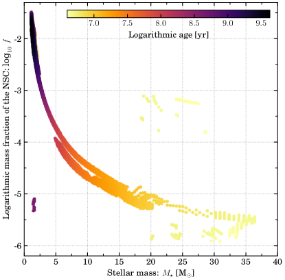
Figure 10: Logarithmic fraction of the number of AGB stars multiplied by their mass and divided by the total nuclear star cluster mass ($\log_{10}\,f$) versus AGB star mass. Each data point is color-coded according to the age of the star. Note that all AGB stars are younger than the main stellar population of the NSC, as identified by fitting the spectral energy distribution.

However, all model AGB stars that satisfy the color-cuts are younger than $5\text{\,}\mathrm{Gyr}$, which gives the lower uncertainty on the age of the main stellar population of the NSC. Therefore, if AGB stars are responsible for the emission in the MIRI data, there must have been star formation in-situ after the initial formation of the NSC.

In case the AGB stars are old, meaning that many AGB stars are required to account for the emission in the mid-infrared, it remains unclear why both the effective radius and ellipticity change significantly, as the cluster with the AGB star should have relaxed between their formation and today. In contrast, only few massive and young AGB stars are required to account for the mid-infrared emission, which could explain the increased effective radius and ellipticity, if they formed outside the center of the NSC. However, this would require in-flow of gas in the past few $\mathrm{Myr}$ but we cannot detect the presence of a young stellar population in the NSC. Therefore, it remains challenging to explain both the structural and photometric parameters using only AGB stars.

5.3.4 A circum-nuclear gaseous disk

Another possibility is that the infrared emission originates from a circum-nuclear gaseous disk or ring with a radius of a few pc, similar to the one present in the MW. Indeed, the MW hosts a clumpy, asymmetric, inhomogeneous, and kinematically disturbed concentration of molecular/ionized gas at $R\lesssim$5\text{\,}\mathrm{pc}$$ known as the circum-nuclear disk (e.g. Lau et al., 2013; Hsieh et al., 2021). The MW circum-nuclear disk occupies similar radii to its NSC, has a total mass of $M_{\mathrm{gas}}^{\mathrm{disk}}\simeq${10}^{4}$$-${10}^{5}\text{\,}\mathrm{M_{\odot}}$ and it is probably a transient structure (on a timescale of few $\mathrm{Myr}$) originating from a series of randomly oriented in-flow events (Requena-Torres et al., 2012). By analogy, we could hypothezise that NGC 628 hosts a similar gaseous structure and that this is producing the observed mid-infrared emission. While the emission from the gas disk could explain the observed photometry, it is unclear why we do not detect a “young” (formed in the last few $\mathrm{Gyr}$) stellar population in the NSC. While the ALMA CO band does not show significant emission in NGC 628’s center (see Figure 1), this may be related to the sensitivity of the ALMA measurements and could not exclude a low-mass disk: in the the PHANGS–ALMA v4p0 “broad” CO (2-1) map, the intensity measurement at the position of the NSC is $I_{(\mathrm{CO})2-1}=(-0.27\pm$1.30$)$\mathrm{K}\text{\,}\mathrm{km}\text{\,}{\mathrm{s}}^{-1}$$. Given the beam size ($\theta=$1.12\text{\,}\arcsec$$) and distance to the target, translating this value to a $$3$\sigma$ upper limit yields to the CO (2-1) luminosity yields $\log_{10}\,L_{(\mathrm{CO})2-1}\,/\,$\mathrm{K}\text{\,}\mathrm{km}\text{\,}{\mathrm{s}}^{-1}\text{\,}{\mathrm{pc}}^{2}$<4.1$. For a standard Milky Way CO to H₂ conversion factor and CO (2–1) to CO (1–0) line ratio appropriate for NGC 628 (Bolatto et al., 2013; den Brok et al., 2021), this luminosity limit corresponds to an upper mass limit of $\log_{10}\,M_{\mathrm{H}_{2}}\,/\,$\mathrm{M_{\odot}}$<4.9$. In comparison, the circum-nuclear disk of the Milky Way has a mass of $M_{\mathrm{gas}}\sim$1.2\text{\times}{10}^{4}\text{\,}\mathrm{M_{\odot}}$$ (Requena-Torres et al., 2012).

5.3.5 Background galaxy

It is also plausible that the emission in the MIRI data originates from a background galaxy, which happens to be aligned with the NSC along the line of sight. Although an alignment of the order $0.1\text{\,}\mathrm{\SIUnitSymbolArcsecond}$ is unlikely, we investigate this scenario further based on the photometry found in the MIRI data.

Hassani et al. (in prep., this issue) investigate the properties of compact sources at $21\text{\,}\mathrm{\SIUnitSymbolMicro m}$ for all four PHANGS–JWST targets for which data are available. Using a dendogram-based algorithm, they find $1271$ compact sources of which $115$ are classified as “potential background sources” (or HZ). This classification was performed using flux density ratios between MIRI bands (their Equations 1 and 2). The MIRI structure coinciding with the NSC of NGC 628 was also classified as a potential background object.

A search in the NASA Extragalactic Database revealed that the $114$ sources were previously detected by the WISE / ALLWISE mission (Wright et al., 2010; Cutri et al., 2013) and all objects were classified as “infrared sources”. While these sources show a galaxy-like morphology at $2\text{\,}\mathrm{\SIUnitSymbolMicro m}$, their detailed properties remain unclear at this point.

To compare to the other potential background objects, we select the measured spectral flux densities for the MIRI bands and subtract the extrapolated emission from the NSC using the SED fit excluding the MIRI data (solid line in Figure 5). While the flux density values compare to other potential background sources, their evolution with wavelength does not: none of the $114$ identified potential background objects follow a similar trend in that the flux densities decrease with increasing wavelength.

Therefore, if the other $114$ sources are background galaxies, the differences in the evolution of flux densities with wavelength suggest that the MIRI emission coinciding with the NSC of NGC 628 is not related to a background galaxy. Such a scenario becomes more unlikely if we combine it with the probability of alignment with the NSC along the line of sight.

6 Conclusions

In this work we analysed the nuclear star cluster (NSC) of NGC 628, a nearby late-type spiral galaxy, with archival Hubble Space Telescope (HST) ACS & WFC3 and newly obtained James Webb Space Telescope (JWST) NIRCam & MIRI data. The combined data cover the ultraviolet to mid-infrared wavelength, enabling an unprecedented analysis of an extragalactic NSC. Our findings can be summarized as follows:

1. Combining the $\mathrm{\textit{B}}-\mathrm{\textit{V}}$ color with various mass-to-light relations results in an NSC stellar mass of $\log_{10}\,(M_{\star}^{\mathrm{nsc}}\,/\,$\mathrm{M_{\odot}}$)=$7.06$\pm$0.31$$. We compare this number to an estimate derived using the K-band magnitude (resulting in $$7.2$\pm$1.1$$) and the results from fitting the spectral energy distribution (SED; resulting in $\sim$7.1$$). These values are consistent with the literature value of $$7.05$\pm$0.21$$ (Georgiev et al., 2016).

2. The effective radius and ellipticity of the NSC are $\sim$5\text{\,}\mathrm{pc}$$ and $\sim$0.05$$, respectively, across the ultraviolet, optical, and near-infrared regime. At the same time the Sérsic index drops from $\sim$3$$ to $\sim$2$$ and the position angle drops from $\sim$130\text{\,}\mathrm{\SIUnitSymbolDegree}$$ to $\sim$90$$-$100\text{\,}\mathrm{\SIUnitSymbolDegree}$. These values supersede literature values, which varied significantly across neighboring bands (Georgiev & Böker, 2014).

3. In the mid-infrared bands, the effective radius and ellipticity increase to $\sim$12\text{\,}\mathrm{pc}$$ and $\sim$0.4$$, respectively. The Sérsic index drops further to $\sim$1.5$$ while being consistent with an exponential profile, and the position angle remains unchanged compared to the near-infrared.

4. We fit the SED from the ultraviolet to the near-infrared with a total of ten data points to find an old stellar population of $($8$\pm$3$)$\mathrm{Gyr}$$ with a metallicity of $Z=$0.012$\pm$0.006$$. The fit indicates that no younger stellar population is present.

5. Fitting the SED with the inclusion of the MIRI data yields an overall worse fit, as evaluated by $\chi^{2}$ statistics. Nevertheless, the age and metallicity of the main stellar population remain unchanged within the uncertainties. The differences in both fits to the SED indicate that the MIRI data do not trace the stellar population found in the lower wavelength regimes.

6. We find different angular separations between the center of the NSC in different bands, being most significant in the mid-infrared data. However, depending on the band from which the world coordinate system is taken as reference, the separations become less significant. This could hint at persistent calibration issues with the world coordinate systems of individual bands.

The color, age, and metallicity of the main stellar population of NGC 628’s NSC indicate that no star formation has taken place in the previous few $\mathrm{Gyr}$ in its center. This is caused either by a dynamical mechanism preventing gas and dust inflow, or by feedback from the center. The lack of a young stellar population hints that the central cavity, which lacks both gas and dust and has a size of approximately $$200\text{\,}\mathrm{pc}$\times$400\text{\,}\mathrm{pc}$$ around the NSC, has existed for the last few $\mathrm{Gyr}$ as well. The reason for the lack of recent in-situ star formation and origin of the central cavity remains unknown.

The nature of the emission in the mid-infrared bands remains a mystery as well. From our SED fits it is clear that the old stellar population of the NSC cannot completely explain the emission in JWST’s MIRI bands. We discussed five different mechanisms, which may cause the emission: (1) contribution from a central active galactic nucleus, (2) an infalling star cluster, (3) dust from asymptotic giant branch (AGB) stars, (4) the presence of a circum-nuclear disk, and (5) alignment with a background galaxy.

The AGB scenario could explain the observed photometry. However, we find that the AGB stars whose colors fit the measurements are younger than the main stellar population. From a comparison to model AGB stars, we find that either a large number of old or a small number of young stars are required. While the first scenario cannot explain the wavelength dependence of the structural parameters, the latter scenario requires recent (a few $\mathrm{Myr}$ ago) in-falling gas, however, no stellar population younger than $5\text{\,}\mathrm{Gyr}$ was detected from SED fitting. In conclusion, none of the four discussed scenarios can fully explain both the structural and photometric measurements.

Our analysis highlights the potential JWST data has for exploring galactic nuclei in the nearby Universe. An ongoing analysis of the stellar population using PHANGS–MUSE data can improve the situation, albeit it cannot resolve the NSC. To solve the riddle of the nucleus of NGC 628 at long wavelengths, we will propose high-resolution spectroscopic observations, ideally Integral Field Unit spectroscopic data with JWST, to determine the kinematic properties of the NSC and its direct surroundings. In addition to the nature of the structure in the mid-infrared bands, these data will constrain further the presence of a young stellar population, the kinematic signature compared to the cluster, and help to constrain the presence of a black hole in NGC 628 as there is currently no available robust mass measurement or upper limit.

Data Availability

The data underlying this article are publicly available at the Milkulski Archive for Space Telescopes (MAST). The specific observations analyzed can be accessed via http://dx.doi.org/10.17909/t9-r08f-dq31 (catalog doi:10.17909/t9-r08f-dq31) and http://dx.doi.org/10.17909/9bdf-jn24 (catalog doi:10.17909/9bdf-jn24).

Appendix A Number of Sérsic profiles

The description of the projected light distribution of NSCs is often approximated by a single simple analytic function such as a Sérsic profile, with few exceptions (Nguyen et al., 2018; Pechetti et al., 2022). With increasing spatial resolution at all wavelength ranges, accurate descriptions of the light distribution of NSCs may warrant multiple profiles. The NSC of NGC 628 was analyzed previously by Georgiev & Böker (2014) and modeled with a single King profile, but the goodness of the fit was not indicated.

Here we explore whether adding a second Sérsic profile improves the fit compared to a single Sérsic profile. The goodness of the two fits may not be compared via the standard $\chi^{2}$ statistics, as different number of free parameters are at play. To compensate for the increased number of free parameters $k$, a penalty is introduced by adding a term linear in $k$ to the standard $\chi^{2}$ evaluation. We use the Bayesian Information Criteria (BIC, Schwarz, 1978), defined as

$$\mathrm{BIC}=-2\ln\,\mathcal{L}+k\ln\,N\;,$$ (A1)

where $\mathcal{L}$ is the likelihood value and $N$ the total number of data points. Model ($A$) is generally preferred over model ($B$) if $\Delta\mathrm{BIC}=\mathrm{BIC}_{B}-\mathrm{BIC}_{A}>0$, but note that the BIC is a heuristic approach and includes approximations.

We highlight the results for the single (labeled “A”) and double Sérsic profile (labeled “B”) fits for the NSC in Table 5. The $F2100W$ is excluded from the list as the fit with two profiles for the NSC did not converge under any circumstance.

The conclusion from this experiment is that a single Sérsic profile is preferred over fitting two Sérsic profiles for the NSC.

Table 5: Differences in the Bayesian Information Criteria ($\Delta\mathrm{BIC}$) between two ($A$) and a single Sérsic profile ($B$) for the NSC of NGC 628.

Band	$\mathrm{BIC}_{(A)}$	$\mathrm{BIC}_{(B)}$	$\Delta\mathrm{BIC}$	$\frac{\mathrm{BIC}_{(A)}}{\mathrm{BIC}_{(B)}}$
$F275W$	$269$	$203$	$66$	$1.33$
$F336W$	$225$	$156$	$69$	$1.44$
$F435W$	$234$	$155$	$79$	$1.51$
$F555W$	$227$	$162$	$65$	$1.40$
$F658N$	$216$	$150$	$66$	$1.44$
$F814W$	$284$	$222$	$62$	$1.28$
$F200W$	$14\,191$	$14\,121$	$70$	$1.00$
$F300M$	$940$	$870$	$70$	$1.08$
$F335M$	$1167$	$1047$	$120$	$1.11$
$F360M$	$1133$	$1105$	$27$	$1.03$
$F770W$	$421$	$343$	$78$	$1.23$
$F1000W$	DNF	$382$	–	–
$F1130W$	DNF	$482$	–	–
$F2100W$	DNF	DNF	–	–

Appendix B Data table

In Table 6 we present the best-fit parameters using a single Sérsic profile.

Table 6: Best-fit parameter estimates for the nuclear star cluster of NGC 628 using a single Sérsic profile. The parameter values and their uncertainties were determined via $500$ bootstrap iterations, where the best-fit value gives the median and the uncertainties the $1\sigma$ interval.

Band	RA	DEC	PA	$\epsilon$	$n$	$r_{\mathrm{eff}}$		$m_{0}$
	[hms]	[dms]	[deg]			[$\mathrm{arcsec}$]	[$\mathrm{pc}$]	[$\mathrm{mag}$]
F275W	01:36:41.742	+15:47:01.167	$139^{+16}_{-25}$	$0.13^{+0.03}_{-0.12}$	$3.5^{+1.0}_{-1.5}$	$0.17^{+0.03}_{-0.14}$	$8.2^{+6.7}_{-6.7}$	$21.38^{+0.31}_{-0.16}$
F336W	01:36:41.742	+15:47:01.173	$125.1^{+5.5}_{-5.7}$	$0.056^{+0.009}_{-0.010}$	$2.07^{+0.10}_{-0.11}$	$0.099^{+0.002}_{-0.002}$	$4.74^{+0.09}_{-0.09}$	$20.18^{+0.02}_{-0.02}$
F435W	01:36:41.743	+15:47:01.174	$106.8^{+5.7}_{-6.1}$	$0.066^{+0.013}_{-0.014}$	$3.01^{+0.19}_{-0.18}$	$0.107^{+0.003}_{-0.003}$	$5.10^{+0.14}_{-0.14}$	$18.54^{+0.02}_{-0.02}$
F555W	01:36:41.738	+15:47:01.216	$89^{+29}_{-23}$	$0.020^{+0.011}_{-0.015}$	$2.51^{+0.20}_{-0.29}$	$0.103^{+0.003}_{-0.003}$	$4.91^{+0.14}_{-0.14}$	$17.89^{+0.04}_{-0.02}$
F658N	01:36:41.736	+15:47:01.186	$105^{+11}_{-10}$	$0.049^{+0.020}_{-0.018}$	$2.91^{+0.21}_{-0.31}$	$0.103^{+0.003}_{-0.005}$	$4.91^{+0.22}_{-0.22}$	$17.45^{+0.04}_{-0.02}$
F814W	01:36:41.738	+15:47:01.227	$118.6^{+7.1}_{-7.2}$	$0.066^{+0.015}_{-0.014}$	$3.21^{+0.28}_{-0.43}$	$0.113^{+0.004}_{-0.005}$	$5.39^{+0.24}_{-0.24}$	$17.12^{+0.04}_{-0.03}$
F200W	01:36:41.741	+15:47:01.133	$81^{+12}_{-12}$	$0.036^{+0.013}_{-0.013}$	$2.26^{+0.15}_{-0.02}$	$0.111^{+0.004}_{-0.004}$	$5.31^{+0.21}_{-0.21}$	$16.54^{+0.27}_{-0.27}$
F300M	01:36:41.738	+15:47:01.177	$96^{+12}_{-10}$	$0.053^{+0.022}_{-0.023}$	$2.21^{+0.23}_{-0.37}$	$0.122^{+0.006}_{-0.007}$	$5.81^{+0.35}_{-0.35}$	$17.41^{+0.25}_{-0.25}$
F335M	01:36:41.737	+15:47:01.219	$103^{+11}_{-3}$	$0.074^{+0.027}_{-0.032}$	$2.12^{+0.21}_{-0.28}$	$0.122^{+0.008}_{-0.010}$	$5.80^{+0.47}_{-0.47}$	$17.54^{+0.25}_{-0.25}$
F360M	01:36:41.741	+15:47:01.223	$95.6^{+7.2}_{-5.8}$	$0.099^{+0.029}_{-0.033}$	$1.88^{+0.18}_{-0.21}$	$0.129^{+0.007}_{-0.008}$	$6.16^{+0.38}_{-0.38}$	$17.65^{+0.25}_{-0.25}$
F770W	01:36:41.733	+15:47:01.294	$86.6^{+4.3}_{-4.5}$	$0.296^{+0.034}_{-0.033}$	$0.63^{+0.08}_{-0.08}$	$0.173^{+0.007}_{-0.007}$	$8.25^{+0.36}_{-0.36}$	$18.53^{+0.02}_{-0.02}$
F1000W	01:36:41.733	+15:47:01.245	$93.2^{+5.0}_{-5.6}$	$0.395^{+0.083}_{-0.045}$	$1.45^{+0.71}_{-0.64}$	$0.250^{+0.015}_{-0.022}$	$11.9^{+1.0}_{-1.0}$	$18.78^{+0.15}_{-0.15}$
F1300W	01:36:41.733	+15:47:01.247	$93.1^{+5.0}_{-3.9}$	$0.393^{+0.071}_{-0.045}$	$1,46^{+0.63}_{-0.40}$	$0.251^{+0.009}_{-0.015}$	$11.99^{+0.72}_{-0.72}$	$18.82^{+0.08}_{-0.08}$
F2100W	01:36:41.728	+15:47:01.231	–	–	–	–	–	$19.51^{+0.68}_{-0.68}$

References

- Adamo et al. (2017) Adamo, A., Ryon, J. E., Messa, M., et al. 2017, The Astrophysical Journal, 841, 131, doi: 10.3847/1538-4357/aa7132
- Agarwal & Milosavljević (2011) Agarwal, M., & Milosavljević, M. 2011, The Astrophysical Journal, 729, 35, doi: 10.1088/0004-637X/729/1/35
- Anand et al. (2021) Anand, G. S., Lee, J. C., Van Dyk, S. D., et al. 2021, Monthly Notices of the Royal Astronomical Society, 501, 3621, doi: 10.1093/mnras/staa3668
- Antonini (2013) Antonini, F. 2013, The Astrophysical Journal, 763, 62, doi: 10.1088/0004-637X/763/1/62
- Antonini (2014) —. 2014, The Astrophysical Journal, 794, 106, doi: 10.1088/0004-637X/794/2/106
- Antonini et al. (2015) Antonini, F., Barausse, E., & Silk, J. 2015, The Astrophysical Journal, 812, 72, doi: 10.1088/0004-637X/812/1/72
- Arca Sedda (2020) Arca Sedda, M. 2020, The Astrophysical Journal, 891, 47, doi: 10.3847/1538-4357/ab723b
- Arca Sedda & Capuzzo-Dolcetta (2014) Arca Sedda, M., & Capuzzo-Dolcetta, R. 2014, Monthly Notices of the Royal Astronomical Society, 444, 3738, doi: 10.1093/mnras/stu1683
- Arca-Sedda & Capuzzo-Dolcetta (2017) Arca-Sedda, M., & Capuzzo-Dolcetta, R. 2017, Monthly Notices of the Royal Astronomical Society, 471, 478, doi: 10.1093/mnras/stx1586
- Arca Sedda & Gualandris (2018) Arca Sedda, M., & Gualandris, A. 2018, Monthly Notices of the Royal Astronomical Society, 477, 4423, doi: 10.1093/mnras/sty922
- Arca Sedda et al. (2020) Arca Sedda, M., Gualandris, A., Do, T., et al. 2020, The Astrophysical Journal Letters, 901, L29, doi: 10.3847/2041-8213/abb245
- Asmus et al. (2015) Asmus, D., Gandhi, P., Hönig, S. F., Smette, A., & Duschl, W. J. 2015, Monthly Notices of the Royal Astronomical Society, 454, 766, doi: 10.1093/mnras/stv1950
- Asplund et al. (2009) Asplund, M., Grevesse, N., Sauval, A. J., & Scott, P. 2009, Annual Review of Astronomy & Astrophysics, 47, 481, doi: 10.1146/annurev.astro.46.060407.145222
- Baldassare et al. (2014) Baldassare, V. F., Gallo, E., Miller, B. P., et al. 2014, The Astrophysical Journal, 791, 133, doi: 10.1088/0004-637X/791/2/133
- Barth et al. (2009) Barth, A. J., Strigari, L. E., Bentz, M. C., Greene, J. E., & Ho, L. C. 2009, The Astrophysical Journal, 690, 1031, doi: 10.1088/0004-637X/690/1/1031
- Baumgardt & Hilker (2018) Baumgardt, H., & Hilker, M. 2018, Monthly Notices of the Royal Astronomical Society, 478, 1520, doi: 10.1093/mnras/sty1057
- Bekki (2007) Bekki, K. 2007, Publications of the Astronomical Society of Australia, 24, 77, doi: 10.1071/AS07008
- Bekki et al. (2006) Bekki, K., Couch, W. J., & Shioya, Y. 2006, The Astrophysical Journal Letters, 642, L133, doi: 10.1086/504588
- Bell et al. (2003) Bell, E. F., McIntosh, D. H., Katz, N., & Weinberg, M. D. 2003, The Astrophysical Journal Series, 149, 289, doi: 10.1086/378847
- Bellazzini et al. (2020) Bellazzini, M., Annibali, F., Tosi, M., et al. 2020, Astronomy & Astrophysics, 634, A124, doi: 10.1051/0004-6361/201937284
- Bittner et al. (2020) Bittner, A., Sánchez-Blázquez, P., Gadotti, D. A., et al. 2020, Astronomy & Astrophysics, 643, A65, doi: 10.1051/0004-6361/202038450
- Böker et al. (2002) Böker, T., Laine, S., van der Marel, R. P., et al. 2002, The Astronomical Journal, 123, 1389, doi: 10.1086/339025
- Böker et al. (1999) Böker, T., van der Marel, R. P., & Vacca, W. D. 1999, The Astronomical Journal, 118, 831, doi: 10.1086/300985
- Bolatto et al. (2013) Bolatto, A. D., Wolfire, M., & Leroy, A. K. 2013, Annual Review of Astronomy and Astrophysics, 51, 207, doi: 10.1146/annurev-astro-082812-140944
- Boquien et al. (2019) Boquien, M., Burgarella, D., Roehlly, Y., et al. 2019, Astronomy & Astrophysics, 622, A103, doi: 10.1051/0004-6361/201834156
- Boyer et al. (2022) Boyer, M. L., Anderson, J., Gennaro, M., et al. 2022, Research Notes of the American Astronomical Society, 6, 191, doi: 10.3847/2515-5172/ac923a
- Bradley et al. (2020) Bradley, L., Sipőcz, B., Robitaille, T., et al. 2020, doi: 10.5281/zenodo.4044744
- Brammer (2022) Brammer, G. 2022, Preliminary updates to the NIRCam photometric calibration, Zenodo, doi: 10.5281/zenodo.7143382
- Bressan et al. (2012) Bressan, A., Marigo, P., Girardi, L., et al. 2012, Monthly Notices of the Royal Astronomical Society, 427, 127, doi: 10.1111/j.1365-2966.2012.21948.x
- Briggs et al. (1980) Briggs, F. H., Wolfe, A. M., Krumm, N., & Salpeter, E. E. 1980, The Astrophysical Journal, 238, 510, doi: 10.1086/158007
- Bruzual & Charlot (2003) Bruzual, G., & Charlot, S. 2003, Monthly Notices of the Royal Astronomical Society, 344, 1000, doi: 10.1046/j.1365-8711.2003.06897.x
- Burgarella et al. (2005) Burgarella, D., Buat, V., & Iglesias-Páramo, J. 2005, Monthly Notices of the Royal Astronomical Society, 360, 1413, doi: 10.1111/j.1365-2966.2005.09131.x
- Butler & Martínez-Delgado (2005) Butler, D. J., & Martínez-Delgado, D. 2005, The Astronomical Journal, 129, 2217, doi: 10.1086/429524
- Calzetti et al. (2015) Calzetti, D., Johnson, K. E., Adamo, A., et al. 2015, The Astrophysical Journal, 811, 75, doi: 10.1088/0004-637X/811/2/75
- Capaccioli (1989) Capaccioli, M. 1989, in World of Galaxies (Le Monde des Galaxies), ed. H. G. Corwin & L. Bottinelli, 208–227. https://ui.adsabs.harvard.edu/abs/1989woga.conf..208C
- Capuzzo-Dolcetta (1993) Capuzzo-Dolcetta, R. 1993, The Astrophysical Journal, 415, 616, doi: 10.1086/173189
- Cardelli et al. (1989) Cardelli, J. A., Clayton, G. C., & Mathis, J. S. 1989, The Astrophysical Journal, 345, 245, doi: 10.1086/167900
- Carlsten et al. (2022) Carlsten, S. G., Greene, J. E., Beaton, R. L., & Greco, J. P. 2022, The Astrophysical Journal, 927, 44, doi: 10.3847/1538-4357/ac457e
- Carollo & Stiavelli (1998) Carollo, C. M., & Stiavelli, M. 1998, The Astronomical Journal, 115, 2306, doi: 10.1086/300373
- Carollo et al. (1997) Carollo, C. M., Stiavelli, M., de Zeeuw, P. T., & Mack, J. 1997, The Astronomical Journal, 114, 2366, doi: 10.1086/118654
- Carollo et al. (2002) Carollo, C. M., Stiavelli, M., Massimo, S., et al. 2002, The Astronomical Journal, 123, 159, doi: 10.1086/324725
- Carson et al. (2015) Carson, D. J., Barth, A. J., Seth, A. C., et al. 2015, The Astronomical Journal, 149, 149, doi: 10.1088/0004-6256/149/5/170
- Cavanagh et al. (2022) Cavanagh, M. K., Bekki, K., Groves, B. A., & Pfeffer, J. 2022, Monthly Notices of the Royal Astronomical Society, 510, 5164, doi: 10.1093/mnras/stab3786
- Chabrier (2003) Chabrier, G. 2003, The Publications of the Astronomical Society of the Pacific, 115, 763, doi: 10.1086/376392
- Chen et al. (2015) Chen, Y., Bressan, A., Girardi, L., et al. 2015, Monthly Notices of the Royal Astronomical Society, 452, 1068, doi: 10.1093/mnras/stv1281
- Chen et al. (2014) Chen, Y., Girardi, L., Bressan, A., et al. 2014, Monthly Notices of the Royal Astronomical Society, 444, 2525, doi: 10.1093/mnras/stu1605
- Chen et al. (2022) Chen, Z., Do, T., Ghez, A. M., et al. 2022, 37. https://arxiv.org/abs/2212.01397
- Chevance et al. (2020) Chevance, M., Kruijssen, J. M. D., Hygate, A. P. S., et al. 2020, Monthly Notices of the Royal Astronomical Society, 493, 2872, doi: 10.1093/mnras/stz3525
- Condon (1987) Condon, J. J. 1987, The Astrophysical Journal Supplement Series, 65, 485, doi: 10.1086/191234
- Côté et al. (2006) Côté, P., Piatek, S., Ferrarese, L., et al. 2006, The Astrophysical Journal Supplement Series, 165, 57, doi: 10.1086/504042
- Crnojević et al. (2016) Crnojević, D., Sand, D. J., Zaritsky, D., et al. 2016, The Astrophysical Journal Letters, 824, L14, doi: 10.3847/2041-8205/824/1/L14
- Cutri et al. (2013) Cutri, R. M., Wright, E. L., Conrow, T., et al. 2013, Explanatory Supplement to the AllWISE Data Release Products. https://wise2.ipac.caltech.edu/docs/release/allwise/expsup/index.html
- Davis et al. (2021) Davis, A. B., Nierenberg, A. M., Peter, A. H. G., et al. 2021, Monthly Notices of the Royal Astronomical Society, 500, 3854, doi: 10.1093/mnras/staa3246
- Decin (2021) Decin, L. 2021, Annual Review of Astronomy and Astrophysics, 59, 337, doi: 10.1146/annurev-astro-090120-033712
- den Brok et al. (2021) den Brok, J. S., Chatzigiannakis, D., Bigiel, F., et al. 2021, Monthly Notices of the Royal Astronomical Society, 504, 3221, doi: 10.1093/mnras/stab859
- den Brok et al. (2014) den Brok, M., Peletier, R. F., Seth, A. C., et al. 2014, Monthly Notices of the Royal Astronomical Society, 445, 2385, doi: 10.1093/mnras/stu1906
- Do et al. (2009) Do, T., Ghez, A. M., Morris, M. R., et al. 2009, The Astrophysical Journal, 703, 1323, doi: 10.1088/0004-637X/703/2/1323
- Do et al. (2015) Do, T., Kerzendorf, W., Winsor, N., et al. 2015, The Astrophysical Journal, 809, 143, doi: 10.1088/0004-637X/809/2/143
- Dong & De Robertis (2006) Dong, X. Y., & De Robertis, M. M. 2006, The Astronomical Journal, 131, 1236, doi: 10.1086/499334
- Dutil & Roy (1999) Dutil, Y., & Roy, J.-R. 1999, The Astrophysical Journal, 516, 62, doi: 10.1086/307100
- Eigenthaler et al. (2018) Eigenthaler, P., Puzia, T. H., Taylor, M. A., et al. 2018, The Astrophysical Journal, 855, 142, doi: 10.3847/1538-4357/aaab60
- Elmegreen & Elmegreen (1984) Elmegreen, D. M., & Elmegreen, B. G. 1984, The Astrophysical Journal Supplement Series, 54, 127, doi: 10.1086/190922
- Emsellem et al. (2022) Emsellem, E., Schinnerer, E., Santoro, F., et al. 2022, Astronomy & Astrophysics, 659, A191, doi: 10.1051/0004-6361/202141727
- Erwin (2015) Erwin, P. 2015, The Astrophysical Journal, 799, 226, doi: 10.1088/0004-637X/799/2/226
- Erwin & Gadotti (2012) Erwin, P., & Gadotti, D. A. 2012, Advances in Astronomy, 2012, 946368, doi: 10.1155/2012/946368
- Fahrion et al. (2022a) Fahrion, K., Leaman, R., Lyubenova, M., & van de Ven, G. 2022a, Astronomy & Astrophysics, 658, A172, doi: 10.1051/0004-6361/202039778
- Fahrion et al. (2020) Fahrion, K., Müller, O., Rejkuba, M., et al. 2020, Astronomy & Astrophysics, 634, A53, doi: 10.1051/0004-6361/201937120
- Fahrion et al. (2021) Fahrion, K., Lyubenova, M., van de Ven, G., et al. 2021, Astronomy & Astrophysics, 650, A137, doi: 10.1051/0004-6361/202140644
- Fahrion et al. (2022b) Fahrion, K., Bulichi, T.-E., Hilker, M., et al. 2022b. https://arxiv.org/abs/2210.01556
- Fathi et al. (2007) Fathi, K., Backman, J. E., Zurita, A., et al. 2007, Astronomy & Astrophysics, 466, 905, doi: 10.1051/0004-6361:20066990
- Feldmeier-Krause et al. (2017a) Feldmeier-Krause, A., Kerzendorf, W., Neumayer, N., et al. 2017a, Monthly Notices of the Royal Astronomical Society, 464, 194, doi: 10.1093/mnras/stw2339
- Feldmeier-Krause et al. (2017b) Feldmeier-Krause, A., Zhu, L., Neumayer, N., et al. 2017b, Monthly Notices of the Royal Astronomical Society, 466, 4040, doi: 10.1093/mnras/stw3377
- Feldmeier-Krause et al. (2015) Feldmeier-Krause, A., Neumayer, N., Schödel, R., et al. 2015, Astronomy & Astrophysics, 584, A2, doi: 10.1051/0004-6361/201526336
- Feldmeier-Krause et al. (2020) Feldmeier-Krause, A., Kerzendorf, W., Do, T., et al. 2020, Monthly Notices of the Royal Astronomical Society, 494, 396, doi: 10.1093/mnras/staa703
- Fensch et al. (2019) Fensch, J., van der Burg, R. F. J., Jeřábková, T., et al. 2019, Astronomy & Astrophysics, 625, A77, doi: 10.1051/0004-6361/201834911
- Ferrarese et al. (2006) Ferrarese, L., Côté, P., Dalla Bontá, E., et al. 2006, The Astronomical Journal, 644, L21, doi: 10.1086/505388
- Ferrarese et al. (2020) Ferrarese, L., Côté, P., MacArthur, L. A., et al. 2020, The Astrophysical Journal, 890, 128, doi: 10.3847/1538-4357/ab339f
- Fitzpatrick (1999) Fitzpatrick, E. L. 1999, The Publication of the Astronomical Society of the Pacific, 111, 63, doi: 10.1086/316293
- Friedli & Benz (1995) Friedli, D., & Benz, W. 1995, Astronomy & Astrophysics, 301, 649. https://ui.adsabs.harvard.edu/abs/1995A%2526A...301..649F
- Fritz et al. (2016) Fritz, T. K., Chatzopoulos, S., Gerhard, O., et al. 2016, The Astrophysical Journal, 821, 44, doi: 10.3847/0004-637X/821/1/44
- Fruchter et al. (2010) Fruchter, A. S., Hack, W., Dencheva, N., Droettboom, M., & Greenfield, P. 2010, in STScI Calibration Workshop, ed. S. Deustua & C. Oliveira (Space Telescope Science Institute), 376–381. https://ui.adsabs.harvard.edu/abs/2010bdrz.conf..382F
- Fruchter & Hook (1997) Fruchter, A. S., & Hook, R. N. 1997, in Applications of Digital Image Processing XX, ed. A. G. Tescher, Vol. 3164, 120–125, doi: 10.1117/12.292751
- Gallego-Cano et al. (2020) Gallego-Cano, E., Schödel, R., Nogueras-Lara, F., et al. 2020, Astronomy & Astrophysics, 634, A71, doi: 10.1051/0004-6361/201935303
- Genzel et al. (2010) Genzel, R., Eisenhauer, F., & Gillessen, S. 2010, Reviews of Modern Physics, 82, 3121, doi: 10.1103/RevModPhys.82.3121
- Georgiev & Böker (2014) Georgiev, I. Y., & Böker, T. 2014, Monthly Notices of the Royal Astronomical Society, 441, 3570, doi: 10.1093/mnras/stu797
- Georgiev et al. (2016) Georgiev, I. Y., Böker, T., Leigh, N., Lützgendorf, N., & Neumayer, N. 2016, Monthly Notices of the Royal Astronomical Society, 457, 2122, doi: 10.1093/mnras/stw093
- Georgiev et al. (2009a) Georgiev, I. Y., Hilker, M., Puzia, T. H., Goudfrooij, P., & Baumgardt, H. 2009a, Monthly Notices of the Royal Astronomical Society, 396, 1075, doi: 10.1111/j.1365-2966.2009.14776.x
- Georgiev et al. (2009b) Georgiev, I. Y., Puzia, T. H., Hilker, M., & Goudfrooij, P. 2009b, Monthly Notices of the Royal Astronomical Society, 392, 879, doi: 10.1111/j.1365-2966.2008.14104.x
- Gonzaga et al. (2012) Gonzaga, S., Hack, W., Fruchter, A., & Mack, J. 2012, The DrizzlePac Handbook. https://ui.adsabs.harvard.edu/abs/2012drzp.book.....G
- Graham & Driver (2005) Graham, A. W., & Driver, S. P. 2005, Publications of the Astronomical Society of Australia, 22, 118, doi: 10.1071/AS05001
- Graham & Spitler (2009) Graham, A. W., & Spitler, L. R. 2009, Monthly Notices of the Royal Astronomical Society, 397, 2148, doi: 10.1111/j.1365-2966.2009.15118.x
- Grasha et al. (2015) Grasha, K., Calzetti, D., Adamo, A., et al. 2015, The Astrophysical Journal, 815, 93, doi: 10.1088/0004-637X/815/2/93
- Green (2018) Green, G. M. 2018, The Journal of Open Source Software, 3, 695, doi: 10.21105/joss.00695
- Groenewegen (2006) Groenewegen, M. A. T. 2006, Astronomy & Astrophysics, 448, 181, doi: 10.1051/0004-6361:20054163
- Guillard et al. (2016) Guillard, N., Emsellem, E., & Renaud, F. 2016, Monthly Notices of the Royal Astronomical Society, 461, 3620, doi: 10.1093/mnras/stw1570
- Hannah et al. (2021) Hannah, C. H., Seth, A. C., Nguyen, D. D., et al. 2021, The Astronomical Journal, 162, 281, doi: 10.3847/1538-3881/ac282e
- Harris et al. (2020) Harris, C. R., Millman, K. J., van der Walt, S. J., et al. 2020, Nature, 585, 357, doi: 10.1038/s41586-020-2649-2
- Hartmann et al. (2011) Hartmann, M., Debattista, V. P., Seth, A. C., Cappellari, M., & Quinn, T. R. 2011, Monthly Notices of the Royal Astronomical Society, 418, 2697, doi: 10.1111/j.1365-2966.2011.19659.x
- Hassani et al. (in prep.) Hassani, H., et al. in prep., ApJL
- Henshaw et al. (2022) Henshaw, J. D., Barnes, A. T., Battersby, C., et al. 2022. https://arxiv.org/abs/2203.11223
- Hoyer et al. (2021) Hoyer, N., Neumayer, N., Georgiev, I. Y., Seth, A. C., & Greene, J. E. 2021, Monthly Notices of the Royal Astronomical Society, 507, 3246, doi: 10.1093/mnras/stab2277
- Hoyer et al. (2022) Hoyer, N., Pinna, F., Kamlah, A. W. H., et al. 2022, The Astrophysical Journal Letters, 26. https://arxiv.org/abs/2211.13997
- Hsieh et al. (2021) Hsieh, P.-Y., Koch, P. M., Kim, W.-T., et al. 2021, The Astrophysical Journal, 913, 94, doi: 10.3847/1538-4357/abf4cd
- Hunter (2007) Hunter, J. D. 2007, Computing in Science & Engineering, 9, 90, doi: 10.1109/MCSE.2007.55
- Into & Portinari (2013) Into, T., & Portinari, L. 2013, Monthly Notices of the Royal Astronomical Society, 430, 2715, doi: 10.1093/mnras/stt071
- Kacharov et al. (2018) Kacharov, N., Neumayer, N., Seth, A. C., et al. 2018, Monthly Notices of the Royal Astronomical Society, 480, 1973, doi: 10.1093/mnras/sty1985
- Kamlah et al. (2022) Kamlah, A. W. H., Spurzem, R., Berczik, P., et al. 2022, Monthly Notices of the Royal Astronomical Society, 516, 3266, doi: 10.1093/mnras/stac2281
- Kamphuis & Briggs (1992) Kamphuis, J., & Briggs, F. 1992, Astronomy & Astrophysics, 253, 335. https://ui.adsabs.harvard.edu/abs/1992A&A...253..335K
- King (1962) King, I. 1962, The Astronomical Journal, 67, 471, doi: 10.1086/108756
- Klessen & Glover (2016) Klessen, R. S., & Glover, S. C. O. 2016, Saas-Fee Advanced Course, 43, 85, doi: 10.1007/978-3-662-47890-5_2
- Koleva et al. (2009) Koleva, M., de Rijcke, S., Prugniel, P., Zeilinger, W. W., & Michielsen, D. 2009, Monthly Notices of the Royal Astronomical Society, 396, 2133, doi: 10.1111/j.1365-2966.2009.14820.x
- Kreckel et al. (2018) Kreckel, K., Faesi, C., Kruijssen, J. M. D., et al. 2018, The Astrophysical Journal Letters, 863, L21, doi: 10.3847/2041-8213/aad77d
- Krist (1993) Krist, J. 1993, in Astronomical Data Analysis Software and Systems II, ed. R. J. Hanisch, R. J. V. Brissenden, & J. Barnes, Vol. 52, 536. https://ui.adsabs.harvard.edu/abs/1993ASPC...52..536K
- Krist (1995) Krist, J. 1995, in Astronomical Data Analysis Software and Systems IV, ed. R. A. Shaw, H. E. Payne, & J. J. E. Hayes, Vol. 77, 349. https://adass.org/adass/proceedings/adass94/kristj.html
- Kroupa (2001) Kroupa, P. 2001, Monthly Notices of the Royal Astronomical Society, 322, 231, doi: 10.1046/j.1365-8711.2001.04022.x
- Krumholz & Kruijssen (2015) Krumholz, M. R., & Kruijssen, J. M. D. 2015, Monthly Notices of the Royal Astronomical Society, 453, 739, doi: 10.1093/mnras/stv1670
- Lang et al. (2020) Lang, P., Meidt, S. E., Rosolowsky, E., et al. 2020, The Astrophysical Journal, 897, 122, doi: 10.3847/1538-4357/ab9953
- Larsen (1999) Larsen, S. S. 1999, Astronomy and Astrophysics Supplement, 139, 393, doi: 10.1051/aas:1999509
- Lau et al. (2013) Lau, R. M., Herter, T. L., Morris, M. R., Becklin, E. E., & Adams, J. D. 2013, The Astrophysical Journal, 775, 37, doi: 10.1088/0004-637X/775/1/37
- Lauer et al. (2005) Lauer, T. R., Faber, S. M., Gebhardt, K., et al. 2005, The Astronomical Journal, 129, 2138, doi: 10.1086/429565
- Launhardt et al. (2002) Launhardt, R., Zylka, R., & Mezger, P. G. 2002, Astronomy & Astrophysics, 384, 112, doi: 10.1051/0004-6361:20020017
- Lee et al. (in prep.) Lee, J., et al. in prep., ApJ
- Leroy et al. (in prep.) Leroy, A., et al. in prep., ApJ
- Leroy et al. (2021) Leroy, A. K., Schinnerer, E., Hughes, A., et al. 2021, The Astrophysical Journal Series, 257, 43, doi: 10.3847/1538-4365/ac17f3
- Lesch et al. (1990) Lesch, H., Biermann, P. L., Crusius, A., et al. 1990, Monthly Notices of the Royal Astronomical Society, 242, 194, doi: 10.1093/mnras/242.2.194
- Loup et al. (1997) Loup, C., Zijlstra, A. A., Waters, L. B. F. M., & Groenewegen, M. A. T. 1997, Astronomy & Astrophysics Supplement series, 125, 419, doi: 10.1051/aas:1997377
- Lynden-Bell & Pringle (1974) Lynden-Bell, D., & Pringle, J. E. 1974, Monthly Notices of the Royal Astronomical Society, 168, 603. https://academic.oup.com/mnras/article/168/3/603/990948
- Marigo et al. (2017) Marigo, P., Girardi, L., Bressan, A., et al. 2017, The Astrophysical Journal, 835, 77, doi: 10.3847/1538-4357/835/1/77
- Martin (1995) Martin, P. 1995, The Astronomical Journal, 109, 2428, doi: 10.1086/117461
- Matthews et al. (1999) Matthews, L. D., Gallagher, J. S., Krist, J. E., et al. 1999, The Astronomical Journal, 118, 208, doi: 10.1086/300909
- McGaugh & Schombert (2014) McGaugh, S. S., & Schombert, J. M. 2014, The Astronomical Journal, 148, 77, doi: 10.1088/0004-6256/148/5/77
- McQuinn et al. (2017) McQuinn, K. B. W., Skillman, E. D., Dolphin, A. E., Berg, D., & Kennicutt, R. 2017, The Astronomical Journal, 154, 51, doi: 10.3847/1538-3881/aa7aad
- Milosavljević (2004) Milosavljević, M. 2004, The Astrophysical Journal Letters, 605, L13, doi: 10.1086/420696
- Mulcahy et al. (2017) Mulcahy, D. D., Beck, R., & Heald, G. H. 2017, Astronomy & Astrophysics, 600, A6, doi: 10.1051/0004-6361/201629907
- Muñoz et al. (2015) Muñoz, R. P., Eigenthaler, P., Puzia, T. H., et al. 2015, The Astrophysical Journal Letters, 813, L15, doi: 10.1088/2041-8205/813/1/L15
- Nardiello et al. (2022) Nardiello, D., Bedin, L. R., Burgasser, A., et al. 2022, Monthly Notices of the Royal Astronomical Society, doi: 10.1093/mnras/stac2659
- Neumayer et al. (2020) Neumayer, N., Seth, A. C., & Böker, T. 2020, The Astronomy and Astrophysics Review, 28, 75, doi: 10.1007/s00159-020-00125-0
- Nguyen et al. (2017) Nguyen, D. D., Seth, A. C., den Brok, M., et al. 2017, The Astrophysical Journal, 836, 237, doi: 10.3847/1538-4357/aa5cb4
- Nguyen et al. (2018) Nguyen, D. D., Seth, A. C., Neumayer, N., et al. 2018, The Astrophysical Journal, 858, 118, doi: 10.3847/1538-4357/aabe2
- Nguyen et al. (2019) —. 2019, The Astrophysical Journal, 872, 104, doi: 10.3847/1538-4357/aafe7a
- Nogueras-Lara (2022) Nogueras-Lara, F. 2022, arXiv e-prints. https://arxiv.org/abs/2208.13218
- Noll et al. (2009) Noll, S., Burgarella, D., Giovannoli, E., et al. 2009, Astronomy & Astrophysics, 507, 1793, doi: 10.1051/0004-6361/200912497
- Norris et al. (2014) Norris, M. A., Kannappan, S. J., Forbes, D. A., et al. 2014, Monthly Notices of the Royal Astronomical Society, 443, 1151, doi: 10.1093/mnras/stu1186
- O’Donnell (1994) O’Donnell, J. E. 1994, The Astrophysical Journal, 422, 158, doi: 10.1086/173713
- Ordenes-Briceño et al. (2018) Ordenes-Briceño, Y., Puzia, T. H., Eigenthaler, P., et al. 2018, The Astrophysical Journal, 860, 4, doi: 10.3847/1538-4357/aac1b8
- Pastorelli et al. (2019) Pastorelli, G., Marigo, P., Girardi, L., et al. 2019, Monthly Notices of the Royal Astronomical Society, 485, 5666, doi: 10.1093/mnras/stz725
- Pastorelli et al. (2020) —. 2020, Monthly Notices of the Royal Astronomical Society, 498, 3283, doi: 10.1093/mnras/staa2565
- Paudel et al. (2011) Paudel, S., Lisker, T., & Kuntschner, H. 2011, Monthly Notices of the Royal Astronomical Society, 413, 1764, doi: 10.1111/j.1365-2966.2011.18256.x
- Paumard et al. (2006) Paumard, T., Genzel, R., Martins, F., et al. 2006, The Astrophysical Journal, 643, 1011, doi: 10.1086/503273
- Pechetti et al. (2020) Pechetti, R., Seth, A. C., Neumayer, N., et al. 2020, The Astrophysical Journal, 900, 32, doi: 10.3847/1538-4357/abaaa7
- Pechetti et al. (2022) Pechetti, R., Seth, A., Kamann, S., et al. 2022, The Astrophysical Journal, 924, 48, doi: 10.3847/1538-4357/ac339f
- Perrin et al. (2014) Perrin, M. D., Sivaramakrishnan, A., Lajoie, C.-P., et al. 2014, in Space Telescopes and Instrumentation 2014: Optical, Infrared, and Millimeter Wave, ed. J. M. Oschmann, M. Clampin, G. G. Fazio, & H. A. MacEwen, Vol. 9143, 91433X, doi: 10.1117/12.2056689
- Perrin et al. (2012) Perrin, M. D., Soummer, R., Elliott, E. M., Lallo, M. D., & Sivaramakrishnan, A. 2012, in Space Telescopes and Instrumentation 2012: Optical, Infrared, and Millimeter Wave, ed. M. C. Clampin, G. G. Fazio, H. A. MacEwen, & J. M. Oschmann, Vol. 8442, 84423D, doi: 10.1117/12.925230
- Piner et al. (1995) Piner, B. G., Stone, J. M., & Teuben, P. J. 1995, The Astrophysical Journal, 449, 508, doi: 10.1086/176075
- Pinna et al. (2021) Pinna, F., Neumayer, N., Seth, A. C., et al. 2021, The Astrophysical Journal, 921, 8, doi: 10.3847/1538-4357/ac158f
- Portinari et al. (2004) Portinari, L., Sommer-Larsen, J., & Tantalo, R. 2004, Monthly Notices of the Royal Astronomical Society, 347, 691, doi: 10.1111/j.1365-2966.2004.07207.x
- Poulain et al. (2021) Poulain, M., Marleau, F. R., Habas, R., et al. 2021, Monthly Notices of the Royal Astronomical Society, 506, 5494, doi: 10.1093/mnras/stab2092
- Querejeta et al. (2021) Querejeta, M., Schinnerer, E., Meidt, S., et al. 2021, Astronomy & Astrophysics, 656, A133, doi: 10.1051/0004-6361/202140695
- Requena-Torres et al. (2012) Requena-Torres, M. A., Güsten, R., Weiss, A., et al. 2012, Astromomy & Astrophysics, 542, L21, doi: 10.1051/0004-6361/201219068
- Robitaille (2019) Robitaille, T. 2019, APLpy v2.0: The Astronomical Plotting Library in Python, doi: 10.5281/zenodo.2567476
- Robitaille & Bressert (2012) Robitaille, T., & Bressert, E. 2012, APLpy: Astronomical Plotting Library in Python. http://ascl.net/1208.017
- Roediger & Courteau (2015) Roediger, J. C., & Courteau, S. 2015, Monthly Notices of the Royal Astronomical Society, 452, 3209, doi: 10.1093/mnras/stv1499
- Rossa et al. (2006) Rossa, J., van der Marel, R. P., Böker, T., et al. 2006, The Astronomical Journal, 132, 1074, doi: 10.1086/505968
- Sakamoto et al. (1999) Sakamoto, K., Okumura, S. K., Ishitzuki, S., & Scoville, N. Z. 1999, The Astrophysical Journal, 525, 691, doi: 10.1086/307910
- Salpeter (1955) Salpeter, E. E. 1955, The Astrophysical Journal, 121, 161, doi: 10.1086/145971
- Sánchez et al. (2011) Sánchez, S. F., Rosales-Ortega, F. F., Kennicutt, R. C., et al. 2011, Monthly Notices of the Royal Astronomical Society, 410, 313, doi: 10.1111/j.1365-2966.2010.17444.x
- Sánchez-Blázquez et al. (2014) Sánchez-Blázquez, P., Rosales-Ortega, F., Diaz, A., & Sánchez, S. F. 2014, Monthly Notices of the Royal Astronomical Society, 437, 1534, doi: 10.1093/mnras/stt1984
- Sánchez-Janssen et al. (2019a) Sánchez-Janssen, R., Côté, P., Ferrarese, L., et al. 2019a, The Astrophysical Journal, 878, 18, doi: 10.3847/1538-4357/aaf4fd
- Sánchez-Janssen et al. (2019b) Sánchez-Janssen, R., Puzia, T. H., Ferrarese, L., et al. 2019b, Monthly Notices of the Royal Astronomical Society, 486, L1, doi: 10.1093/mnrasl/slz008
- Scarano & Lépine (2013) Scarano, S., & Lépine, J. R. D. 2013, Monthly Notices of the Royal Astronomical Society, 428, 625, doi: 10.1093/mnras/sts048
- Schinnerer et al. (2019) Schinnerer, E., Hughes, A., Leroy, A., et al. 2019, The Astrophysical Journal, 887, 49, doi: 10.3847/1538-4357/ab50c2
- Schlafly & Finkbeiner (2011) Schlafly, E. F., & Finkbeiner, D. P. 2011, The Astrophysical Journal, 737, 103, doi: 10.1088/0004-637X/737/2/103
- Schlegel et al. (1998) Schlegel, D. J., Finkbeiner, D. P., & Davis, M. 1998, The Astrophysical Journal, 500, 525, doi: 10.1086/305772
- Schödel et al. (2014a) Schödel, R., Feldmeier, A., Kunneriath, D., et al. 2014a, Astronomy & Astrophysics, 566, A47, doi: 10.1051/0004-6361/201423481
- Schödel et al. (2014b) —. 2014b, Astronomy & Astrophysics, 566, A47, doi: 10.1051/0004-6361/201423481
- Schödel et al. (2020) Schödel, R., Nogueras-Lara, F., Gallego-Cano, E., et al. 2020, Astronomy & Astrophysics, 641, A102, doi: 10.1051/0004-6361/201936688
- Schwarz (1978) Schwarz, G. 1978, Annals of Statistics, 6, 461. https://ui.adsabs.harvard.edu/link_gateway/1978AnSta...6..461S
- Scott & Graham (2013) Scott, N., & Graham, A. W. 2013, The Astrophysical Journal, 763, 76, doi: 10.1088/0004-637X/763/2/76
- Seigar (2002) Seigar, M. S. 2002, Astronomy & Astrophysics, 393, 499, doi: 10.1051/0004-6361:20021060
- Sérsic (1968) Sérsic, J. L. 1968, Atlas de Galaxias Australes (Universidad Nacional de Cordoba). https://ui.adsabs.harvard.edu/abs/1968adga.book.....S
- Seth et al. (2008) Seth, A. C., Blum, R., Bastian, N., Caldwell, N., & Debattista, V. P. 2008, The Astrophysical Journal, 687, 997, doi: 10.1086/591935
- Seth et al. (2006) Seth, A. C., Dalcanton, J. J., Hodge, P. W., & Debattista, V. P. 2006, The Astronomical Journal, 132, 2539, doi: 10.1086/508994
- Shakura & Sunyaev (1973) Shakura, N. I., & Sunyaev, R. A. 1973, Astronomy & Astrophysics, 24, 337. https://ui.adsabs.harvard.edu/abs/1973A&A....24..337S
- She et al. (2017) She, R., Ho, L. C., & Feng, H. 2017, The Astrophysical Journal, 835, 223, doi: 10.3847/1538-4357/835/2/223
- Sheth et al. (2005) Sheth, K., Vogel, S. N., Regan, M. W., Thornley, M. D., & Teuben, P. J. 2005, The Astrophysical Journal, 632, 217, doi: 10.1086/432409
- Shlosman et al. (1990) Shlosman, I., Begelman, M. C., & Frank, J. 1990, Nature, 345, 679, doi: 10.1038/345679a0
- Sil’chenko & Moiseev (2006) Sil’chenko, O. K., & Moiseev, A. V. 2006, The Astronomical Journal, 131, 1336, doi: 10.1086/499945
- Sirianni et al. (2005) Sirianni, M., Lee, M. J., Benítez, N., et al. 2005, The Publications of the Astronomical Society of the Pacific, 117, 1049, doi: 10.1086/444553
- Sormani et al. (2015) Sormani, M. C., Binney, J., & Magorian, J. 2015, Monthly Notices of the Royal Astronomical Society, 449, 2421, doi: 10.1093/mnras/stv441
- Sormani & Li (2020) Sormani, M. C., & Li, Z. 2020, Monthly Notices of the Royal Astronomical Society, 494, 6030, doi: 10.1093/mnras/staa1139
- Sormani et al. (2020) Sormani, M. C., Tress, R. G., Glover, S. C. O., et al. 2020, Monthly Notices of the Royal Astronomical Society, 497, 5024, doi: 10.1093/mnras/staa1999
- Spengler et al. (2017) Spengler, C., Côté, P., Roediger, J., et al. 2017, The Astrophysical Journal, 849, 55, doi: 10.3847/1538-4357/aa8a78
- Spinoso et al. (2017) Spinoso, D., Bonoli, S., Dotti, M., et al. 2017, Monthly Notices of the Royal Asronomical Society, 465, 3729, doi: 10.1093/mnras/stw2934
- Stone et al. (2017) Stone, N. C., Küpper, A. H. W., & Ostriker, J. P. 2017, Monthly Notices of the Royal Astronomical Society, 467, 4180, doi: 10.1093/mnras/stx097
- Storchi-Bergmann & Schnorr-Müller (2019) Storchi-Bergmann, T., & Schnorr-Müller, A. 2019, Nature Astronomy, 3, 48, doi: 10.1038/s41550-018-0611-0
- Storn & Price (1997) Storn, R., & Price, K. 1997, Journal of Global Optimization, 11, 341, doi: 10.1023/A:1008202821328
- Su et al. (2021) Su, A. H., Salo, H., Janz, J., et al. 2021, Astronomy & Astrophysics, 647, A100, doi: 10.1051/0004-6361/202039633
- Sun et al. (2018) Sun, J., Leroy, A. K., Schruba, A., et al. 2018, The Astrophysical Journal, 860, 172, doi: 10.3847/1538-4357/aac326
- Tang et al. (2014) Tang, J., Bressan, A., Rosenfield, P., et al. 2014, Monthly Notices of the Royal Astronomical Society, 445, 4287, doi: 10.1093/mnras/stu2029
- The Astropy Collaboration et al. (2013) The Astropy Collaboration, Robitaille, T. P., Tollerud, E. J., et al. 2013, Astronomy & Astrophysics, 558, A33, doi: 10.1051/0004-6361/201322068
- The Astropy Collaboration et al. (2018) The Astropy Collaboration, Price-Whelan, A. M., Sipőcz, B. M., et al. 2018, The Astrophysical Journal, 156, 123, doi: 10.3847/1538-3881/aabc4f
- Trabucchi et al. (2021) Trabucchi, M., Wood, P. R., Mowlavi, N., et al. 2021, Monthly Notices of the Royal Astronomical Society, 500, 1575, doi: 10.1093/mnras/staa3356
- Tremaine et al. (1975) Tremaine, S. D., Ostriker, J. P., & Spitzer, L. 1975, The Astrophysical Journal, 196, 407, doi: 10.1086/153422
- Tress et al. (2020) Tress, R. G., Sormani, M. C., Glover, S. C. O., et al. 2020, Monthly Notices of the Royal Astronomical Society, 499, 4455, doi: 10.1093/mnras/staa3120
- Turner et al. (2021) Turner, J. A., Dale, D. A., Lee, J. C., et al. 2021, Monthly Notices of the Royal Astronomical Society, 502, 1366, doi: 10.1093/mnras/stab055
- Turner et al. (2012) Turner, M. L., Côté, P., Ferrarese, L., et al. 2012, The Astrophysical Journal Series, 203, 5, doi: 10.1088/0067-0049/203/1/5
- van Loon et al. (1998) van Loon, J. T., Zijlstra, A. A., Whitelock, P. A., et al. 1998, Astronomy & Astrophysics, 329, 169. https://arxiv.org/abs/9709119
- Venhola et al. (2018) Venhola, A., Peletier, R., Laurikainen, E., et al. 2018, Astronomy & Astrophysics, 620, A165, doi: 10.1051/0004-6361/201833933
- Vílchez et al. (2019) Vílchez, J. M., Relaño, M., Kennicutt, R., et al. 2019, Monthly Notices of the Royal Astronomical Society, 483, 4968, doi: 10.1093/mnras/sty3455
- Walcher et al. (2006) Walcher, C.-J., Böker, T., Charlot, S., et al. 2006, The Astrophysical Journal, 649, 692, doi: 10.1086/505166
- Willmer (2018) Willmer, C. N. A. 2018, The Astrophysical Journal Supplement, 236, 47, doi: 10.3847/1538-4365/aabfdf
- Wright et al. (2010) Wright, E. L., Eisenhardt, P. R. M., Mainzer, A. K., et al. 2010, The Astronomical Journal, 140, 1868, doi: 10.1088/0004-6256/140/6/1868
- Yadav et al. (2021) Yadav, J., Das, M., Patra, N. N., et al. 2021, The Astrophysical Journal, 914, 54, doi: 10.3847/1538-4357/abf8c1
- Yang et al. (2020) Yang, G., Boquien, M., Buat, V., et al. 2020, Monthly Notices of the Royal Astronomical Society, 491, 740, doi: 10.1093/mnras/stz3001
- Yang et al. (2022) Yang, G., Boquien, M., Brandt, W. N., et al. 2022, The Astrophysical Journal, 927, 192, doi: 10.3847/1538-4357/ac4971
- Zanatta et al. (2021) Zanatta, E., Sánchez-Janssen, R., Chies-Santos, A. L., de Souza, R. S., & Blakeslee, J. P. 2021, Monthly Notices of the Royal Astronomical Society, 508, 986, doi: 10.1093/mnras/stab2348
- Zaragoza-Cardiel et al. (2019) Zaragoza-Cardiel, J., Fritz, J., Aretxaga, I., et al. 2019, Monthly Notices of the Royal Astronomical Society, 487, L61, doi: 10.1093/mnrasl/slz093
- Zibetti et al. (2009) Zibetti, S., Charlot, S., & Rix, H.-W. 2009, Monthly Notices of the Royal Astronomical Society, 400, 1181, doi: 10.1111/j.1365-2966.2009.15528.x