Picking on the Same Person:
Does Algorithmic Monoculture lead to Outcome Homogenization?

Abstract

As the scope of machine learning broadens, we observe a recurring theme of algorithmic monoculture: the same systems, or systems that share components (e.g. training data), are deployed by multiple decision-makers. While sharing offers clear advantages (e.g. amortizing costs), does it bear risks? We introduce and formalize one such risk, outcome homogenization: the extent to which particular individuals or groups experience negative outcomes from all decision-makers. If the same individuals or groups exclusively experience undesirable outcomes, this may institutionalize systemic exclusion and reinscribe social hierarchy. To relate algorithmic monoculture and outcome homogenization, we propose the component-sharing hypothesis: if decision-makers share components like training data or specific models, then they will produce more homogeneous outcomes. We test this hypothesis on algorithmic fairness benchmarks, demonstrating that sharing training data reliably exacerbates homogenization, with individual-level effects generally exceeding group-level effects. Further, given the dominant paradigm in AI of foundation models, i.e. models that can be adapted for myriad downstream tasks, we test whether model sharing homogenizes outcomes across tasks. We observe mixed results: we find that for both vision and language settings, the specific methods for adapting a foundation model significantly influence the degree of outcome homogenization. We conclude with philosophical analyses of and societal challenges for outcome homogenization, with an eye towards implications for deployed machine learning systems.

1 Introduction

Machine learning is built on strong traditions of sharing: we share datasets (e.g. ImageNet), models (e.g. BERT), libraries (e.g. PyTorch), optimizers (e.g. Adam), evaluations (e.g. SuperGLUE) and much more. This ethos of sharing serves the field well: we are able to repeatedly capitalize on the effort required to build high-quality assets (e.g. ImageNet has supported thousands of researchers in computer vision), and improvements to these assets have sweeping benefits (e.g. BERT raised all boats in NLP). Yet does sharing also have risks? Could this core institution of the field lead to undesirable outcomes?

We observe that certain forms of sharing can be reinterpreted as monoculture: Kleinberg and Raghavan (2021) define algorithmic monoculture as the state "in which many decision-makers all rely on the [exact] same algorithm." In parts of society where algorithmic systems are ubiquitous, we see trends towards such monoculture Moore and Tambini (2018); Engler (2021). Monocultures often pose serious risks: Kleinberg and Raghavan (2021) show monoculture is suboptimal for decision-makers when their decisions are interconnected, as when they compete to hire job candidates. In ML, our sharing practices often are more complex than sharing the entire algorithmic system: should we think of our practices of sharing assets in ML as monoculture and, if so, what harms should we worry about?

We investigate this question by introducing the risk of outcome homogenization, i.e. the phenomenon of individuals (or groups) exclusively receiving negative outcomes from all decision-makers they interact with. For example, a job applicant may be rejected from every job they apply to due to the use of similar algorithmic resume screening systems at all companies. Homogeneous outcomes, especially in certain high-stakes settings, constitute serious harms to individuals: someone who is rejected from every employment opportunity, or denied admission at every school, may be severely compromised (e.g. unable to provide for their family, unable to secure an education). We view outcome homogenization as an important class of systemic harms that arise when we study social systems, i.e. harms that require observing how individuals are treated by many decision-makers. In § 2, we conceptually motivate outcome homogenization in the context of (algorithmic) hiring. In § 3, we introduce the first mathematical formalism for outcome homogenization: we measure homogenization as the observed probability of systemic failure normalized by a base rate.

To link the social practice of sharing in ML with the social harm of outcome homogenization, we pose and test the component-sharing hypothesis. If decision-makers share the same underlying components, such as training data and machine learning models, then they will tend to systematically fail the same individuals or groups. In reasoning about the sharing of components, we broaden the initial definition of algorithmic monoculture from Kleinberg and Raghavan (2021): monoculture is not just when decision-makers deploy the exact same system, but also when they deploy similar systems (here, meaning similar in how they were constructed). We investigate how two types of shared components — training data and foundation models — contribute to homogeneous outcomes.

In § 4, we demonstrate that data sharing often homogenizes outcomes for individuals and for racial groups across 3 algorithmic fairness datasets. In § 5, we discuss how the rise of foundation models (Bommasani et al., 2021), i.e. models that can be adapted to myriad downstream tasks, could yield unprecedented homogenization. Based on experiments with foundation models for vision (CLIP) and language (RoBERTa), to our surprise, we find the use of foundation models does not always exacerbate outcome homogenization. Instead, we find the specific mechanism for adapting the foundation model to the downstream task significantly influences homogenization: for example, linear probing consistently leads to more homogeneous outcomes than finetuning for both modalities. Through these experiments, it is clear that the relationship between sharing and homogenization is not fully explained by our hypothesis, but that there is some evidence that sharing homogenizes outcomes. To advance the study of homogenization, we conclude with philosophical analysis through an Andersonian relational egalitarian lens (§ 6.1), practical challenges for its diagnosis, measurement, and rectification (§ 6.2) and future directions for the research community (§ 7).

2 Outcome Homogenization in Hiring

To illustrate outcome homogenization and its potential causes (including algorithmic monoculture), we consider the motivating example of hiring, specifically the resume screening phase. Companies use resumes to screen job applicants, choosing which candidates to interview and which to reject. Maximum homogenization occurs when every company makes the same decision about each candidate, such that each lucky candidate is interviewed by all companies and each unlucky candidate by no companies. We say that the unlucky candidates who receive no interviews experience a systemic failure.

What factors might homogenize outcomes in human decision-making? Even in the absence of algorithms, we observe homogeneous outcomes in many settings. In hiring, historically, hiring managers at each company decided who to interview and often agreed in their decisions. This agreement can be attributed to multiple sources: first, if the needs of each company were identical, then managers at different companies may be incentivized to interview the same candidates, thereby homogenizing outcomes. Second, if hiring managers’ choices are influenced by the same social biases, they will mistakenly reject similar people (e.g. those belonging to marginalized groups), thereby contributing to homogenization. Bias in resume screening is well-documented and remains significant (Jowell and Prescott-Clarke, 1970; Bertrand and Mullainathan, 2004; Kline et al., 2021, inter alia).

However, neither explanation implies that systemic failures are inevitable. Companies have different needs, and resumes are imperfect predictors of success in role, so the “best" candidates will likely differ across companies. Further, bias is not uniform across companies: Kline et al. (2021) find that 21% of firms were responsible for 46% of the racial bias in interview decisions. Even if decisions are influenced by the same group-level biases, different companies may choose different individual members of the advantaged and disadvantaged groups. Variance in company needs, in prevalence of bias, and in individual hiring manager preferences all make it more likely that different resumes survive the screening stage at different companies, ensuring some heterogeneity/diversity in resume screening outcomes.

How do these dynamics change with the introduction of algorithmic decision-making? Algorithmic resume screening is ubiquitous: many large companies deploy resume screening algorithms to parse resumes and inform/decide which applicants advance (Sonderling et al., 2022). As a stylized example, if every company deploys the same deterministic system and has the same hiring criteria, then outcomes will be necessarily homogeneous: individuals will either receive interviews at every company or be rejected by all of them (i.e. systemic failure). While this may seem unlikely (i.e. different companies, especially competitors, relying on the same algorithmic system), we observe that many companies rely on third-party vendors to provide these algorithmic hiring tools. Hence, while the status quo is likely more complex than this stylized example (e.g. vendors could customize the algorithms it uses for each client, each client may integrate a vendor’s recommendation with other information sources to make a decision), we do observe that a few major vendors dominate the marketplace for algorithmic resume screening (e.g. 700 companies, including over 30% of Fortune 100 companies, rely on Hirevue Hirevue (2021)). This practice of different decision-makers deploying the same system is defined as algorithmic monoculture by Kleinberg and Raghavan (2021).

More generally, different companies may instead deploy similar, but non-identical, systems. We expand the definition of algorithmic monoculture to encapsulate this broader setting, which is also alluded to in Kleinberg and Raghavan (2021). Engler (2021) describes this as the reality for college enrollment management algorithms, writing "there are a relatively small number (between 5 and 10) of prominent vendors in the enrollment management algorithm market, …their process and analytics are markedly similar. Since their processes seem relatively consistent, the outcomes might be as well — potentially leading to consistently good results for students who match the historical expectations of colleges, and consistently poor results for students who don’t".

Component-sharing hypothesis. In this work, we study systems that are related in how they are constructed, akin to what is described by Engler (2021). We pose the component-sharing hypothesis that relates such algorithmic monoculture with outcome homogenization: If deployed algorithmic systems share components, outcome homogenization will increase (i.e. there will be more systemic failures). In this work, we empirically test this hypothesis for two prominent forms of component sharing: (i) the sharing of training data in training all deployed systems (§ 4) and (ii) the sharing of the same foundation model for building all deployed systems (§ 5).

3 Formalizing Outcome Homogenization

While prior work (Kleinberg and Raghavan, 2021; Creel and Hellman, 2022) alludes to outcome homogenization, here we provide the first mathematical formalism of outcome homogenization. In line with our running example of resume screening, we first formalize outcome homogenization for individuals in terms of systemic failures. We then generalize to the group setting, where groups are systemically excluded rather than individuals. Since homogenization is a concept we introduce in this work, having formally defined our metrics, we relate our homogenization metrics to established metrics for correlation, fairness, robustness, and accuracy.

3.1 Homogeneous Outcomes for Individuals

Setup. Since we define outcome homogenization as a systemic phenomenon, we consider a social system of individuals (e.g. job applicants) and decision-makers (e.g. employers). In this system, we will assume that each individual $j$ interacts with every decision-maker $i$. In the context of machine learning, we will say each decision-maker $i$ is represented by a machine learning model $h^{i}$, though our formalism of homogenization does not depend on the nature of this model (or even that it is a model; our measures apply equally to human decision-making).

As an example, an individual $j\in[N]$ submits features $x_{j}^{i}$ (e.g. their resume) as input to company $i\in[k]$ to receive an outcome $h^{i}(x_{j}^{i})=\hat{y}_{j}^{i}$ (e.g. an interview). Let $D^{i}$ be the empirical distribution of inputs $x^{i}$ for company $i$.

Failures. Let $F^{i}(x_{j}^{i})$ indicate if $\hat{y}_{j}^{i}$ is a failure, i.e. individual $j$ experiences a negative outcome from model $h^{i}$. The failure rate for model $h^{i}$ is

$$\textsc{fail}(h^{i})\triangleq\mathop{\mathbb{E}}_{x^{i}\sim D^{i}}F^{i}(x^{i})=\Pr_{x^{i}\sim D^{i}}\left[F^{i}(x^{i})=1\right].$$ (1)

In classification, failures can be classification errors ($F^{i}(x^{i})\triangleq\mathbb{I}\left[h^{i}(x^{i})\neq y^{i}\right]$): in this case, the failure rate is simply the empirical classification error. In our experiments, we will operate in the classification setting, though other settings can be accommodated by this framing (e.g. in hiring and education, there may not be a "ground truth"; the relevant notion of individual harm to consider may instead be the rate of rejection from opportunities $F^{i}(x^{i})~{}\triangleq~{}\mathbb{I}\left[h^{i}(x^{i})=-1\right]$).

Systemic failures for individuals. If an individual exclusively experiences failure, we say they experience systemic failure. The observed rate of systemic failure $\textsc{systemic failure}(h_{1},\dots,h_{k})$ is

$$\textsc{systemic failure}(h_{1},\dots,h_{k})\triangleq\mathop{\mathbb{E}}_{j}\left[\prod_{i}F^{i}(x_{j}^{i})\right]=\Pr_{j}\left[F^{1}(x_{j}^{1})=1\wedge\dots\wedge F^{k}(x_{j}^{k})=1\right].$$ (2)

Homogenization metric for individuals. systemic failure quantifies homogeneous outcomes, but is difficult to compare across systems with different underlying accuracies: systemic failure will in general be higher for less accurate systems independent of a specific tendency to pick (i.e. fail) on the same person. While we may sometimes want to combine accuracy and outcome homogenization into an overall measure of utility or social welfare, which $\textsc{systemic failure}(h_{1},\dots,h_{k})$ implicitly does, we focus on a relative measure of homogenization that aims to disentangle accuracy from homogenization. Thinking about the societal impact of ML, we are interested in outcome homogenization even, and perhaps especially, when models are highly accurate. That is, we should not neglect those individuals who are failed uniformly merely because the overall system-wide accuracy suggests a rosy picture.

As a result, we measure individual-level outcome homogenization for a social system $\left\{h^{i}\right\}_{i=1}^{k}$ by normalizing the observed rate of systemic failure by the expected rate of systemic failure.

$$\text{$H^{\textbf{individual}}$}(h^{1},\dots,h^{k})\triangleq\frac{\textsc{systemic failure}(h_{1},\dots,h_{k})}{\prod\limits_{i}\textsc{fail}(h^{i})}=\frac{\mathop{\mathbb{E}}\limits_{j}\left[\prod\limits_{i}F^{i}(x_{j}^{i})\right]}{\prod\limits_{i}\left[\mathop{\mathbb{E}}\limits_{j}F^{i}(x_{j}^{i})\right]}$$ (3)

This measure is the ratio between (i) the probability that an individual experiences systemic failure and (ii) the probability that randomly sampled outputs for each model are all failures. That is, the measure captures how the rate of systemic failure changes when we attend to the structure of individuals.

3.2 Homogeneous Outcomes for Groups

In addition to individual-level homogenization, we also measure group-level homogenization. While our individual-level metric individualizes harm, complementing work on group-level biases, we may also want to identify the extent to which (possibly marginalized) social groups (e.g. Black women) are systemically excluded. Further, we often lack individual-level information (e.g. due to privacy concerns; see § 6), or study algorithmic deployments that do not share individuals (e.g. hiring in different states).

Groups. For each input $x^{i}$, denote the associated group as $G(x^{i})\in\mathcal{G}$. Group identity can correspond to the data producer (e.g. the age of a user querying a search engine) or the data subject (e.g. the race of an individual subject to face recognition). Let $D^{i}_{g}$ be the empirical distribution of inputs for group $g$ (i.e. $\{x^{i}\mid G(x^{i})=g\}$). The group failure rate $\textsc{fail}_{g}(h^{i})$ is

$$\textsc{fail}_{g}(h^{i})\triangleq\mathop{\mathbb{E}}_{x^{i}\sim D^{i}_{g}}F^{i}(x^{i}).$$ (4)

Homogenization metric for groups. To measure group-level homogenization, we modify our individual-level metric: a weighted average over groups replaces the simple average over individuals.

$$\text{$H_{G}^{\textbf{group}}$}(h^{1},\dots,h^{k}) =\frac{{\sum\limits_{g}}\left[W(g)\prod\limits_{i}\textsc{fail}_{g}(h^{i})\right]}{\prod\limits_{i}\textsc{fail}(h^{i})}$$ (5)

Weights. We consider three weighting schemes, specified by categorical probability distributions $W$ distributed over $\mathcal{G}$ (full definitions in § A.1):

Average ($H_{\textbf{avg}}$)

$W$ weights each group proportional to its frequency across all deployments.

Uniform ($H_{\textbf{unif}}$)

$W$ is the uniform distribution, so $W(g)=\frac{1}{|\mathcal{G}|}$.

Worst ($H_{\textbf{worst}}$)

$W$ assigns weight $1$ to the group $g_{\textbf{worst}}$ with the highest systemic failure rate and $0$ to all other groups. This reduces the numerator to simply be the systemic failure rate for $g_{\textbf{worst}}$.

We introduce these weight functions to clarify that, much like having both individual-level metrics and group-level metrics, we may want to weight groups differently in different circumstances. For example, weighting by frequency may provide a useful overall measurement of homogenization but obscure systemic exclusion experienced by minority groups or specifically the worst-off group.

3.3 Understanding Our Metrics

As a ratio of probabilities, our metrics take values in $[0,\infty)$ where $0$ indicates no systemic failures, $1$ indicates the observed rate matches the expected rate, and values greater than $1$ indicate homogeneous outcomes beyond what can be expected from the underlying failure rates . In the individual setting, we assume each individual interacts exactly once with each decision-maker, which may not hold in practice (e.g. people may apply multiple times or not apply at all to a given company). We appropriately generalize our individual-level metric to address this in Appendix A. Further, in the group setting, we recover the individual-level metric using the uniform weighting (or the average weighting) if each individual’s inputs are treated as belonging to their own group.

3.4 Relationship with Other Metrics

Since we introduce (several) metrics, we consider how they relate to metrics for related constructs (e.g. accuracy, fairness, robustness). This speaks to the convergent and divergent validity of our metrics (Campbell and Fiske, 1959; Messick, 1987; Jacobs and Wallach, 2021), i.e. whether they are adequately correlated with metrics of similar constructs and adequately uncorrelated with metrics of dissimilar constructs. Here, we discuss theoretical relationships, whereas in § 5.2 we look at the empirical correlations.

Accuracy. When failures are errors, we design our metrics to minimize (anti-)correlation with accuracy. While not theoretically guaranteed, we empirically demonstrate this in Table 1. With that said, we expect there will be settings where the two are correlated: our goal is not to forcibly (i.e. mechanically) ensure no correlation in the technical sense, but to ensure that we do not neglect homogeneous outcomes in highly accurate systems (i.e. neglect the individuals who are systemically failed even when the overall picture may seem favorable).

Fairness and robustness. Beyond accuracy, outcome homogenization in the group setting is closely related to fairness and robustness. However, we emphasize that outcome homogenization is fundamentally about correlated outcomes for social systems, whereas almost all robustness or fairness metrics are defined for a single model. Further, almost all formalisms of fairness and robustness necessitate groups (even if these groups need not be specified in advance), whereas our formalism of homogenization is attractive in that it can be meaningfully defined for singular individuals. Recent work (Zhao and Chen, 2019; D’Amour et al., 2020; Wang et al., 2021) has initiated the study of fairness in multi-task learning, however these works focus on favorable overall trade-offs across tasks as opposed to systemic modes of failure. Conversely, our metrics cease to be interesting (e.g. $H^{\textbf{individual}}$ is always $1$) when there is a single decision-maker as systemic failures degenerate to single-model failures.

At a more fine-grained level, algorithmic fairness metrics (e.g.  Dwork et al., 2012; Hardt et al., 2016) emphasize discrepancies between individuals/groups. In contrast, our metrics do not (explicitly) center these differences: we are interested in the observed rate of systemic failures (and whether this exceeds the expected rate). Performance disparities are not sufficient for outcome homogenization: if the performance disparities across decision-makers do not align, then outcomes may not be homogeneous. For robustness metrics, our metric $H_{\textbf{worst}}$in the worst-case setting closely resembles the metrics studied in work on worst-group robustness (e.g.  Sagawa* et al., 2020). In particular, when there is only one decision-maker, our metric recovers the standard worst-group error normalized by the overall error.

3.5 Alternative Metrics

In Appendix A, we more extensively discuss desiderata for our metric, alternatives we considered, and how we arrived at the metrics we present in the main paper. With that said, we also note conditions where we may instead favor alternatives, as well as connections to familiar quantities like the covariance, Pearson correlation, and (pointwise) mutual information in the binary setting ($k=2$).

4 Data-sharing Experiments

Having stated our mathematical formalism and metrics for outcome homogenization, we test if sharing training data leads to outcome homogenization. We consider widely used algorithmic fairness datasets (Fabris et al., 2022). While demonstrating systemic failures for these specific datasets may not signify concerns of immediate/direct social consequence, these datasets do represent relevant social contexts where other forms of inequity have been documented.

Data. We work with two datasets: German Credit (GC; Dua and Graff, 2017), the third most widely used fairness dataset, and ACS PUMS (Ding et al., 2021), which was built to replace the most widely used fairness dataset, UCI Adult. GC contains information on 1000 German contracts (e.g. credit history, credit amount, credit risk for the individual): following Wang et al. (2021), we consider two prediction tasks of (i) predicting if an individual receives a good or bad loan and (ii) predicting whether their credit amount exceeds 2000. ACS PUMS contains US Census survey data recording 286 features (e.g. self-reported race and sex, occupation, average hours worked per week) for 3.6 million individuals. Ding et al. (2021) construct several prediction tasks of which we use three: (i) predict if an individual is employed, (ii) predict an individual’s income normalized by the poverty threshold, and (iii) predict if an individual has health insurance.

Individuals and groups. For both datasets, we have individual-level information, hence we measure individual-level homogenization. For ACS PUMS, we have self-identified racial demographic metadata across 9 US Census categories (e.g. American Indian, Asian, Black/African American, White, two or more races), hence we measure group-level racial homogenization.

Experimental design. To test if and how data sharing influences outcome homogenization, informally, we would like to specify settings with different amounts of shared data to test how this affects outcomes. However, in general, it is challenging to precisely articulate what it means to "share data" and, therefore, convincingly ensure that one setting involves more sharing than the other. To address this challenge, we present a highly controlled comparison specifying two sampling protocols for the training data: fixed and disjoint. In the fixed setting, we sample $n$ points without replacement from the entire training dataset, which we use to train all of the $k$ task-specific models ($k=2$ for GC and $k=3$ for ACS PUMS). In the disjoint setting, we sample $kn$ points without replacement that we randomly partition across the $k$ task-specific models. In other words, in the fixed setting, the task-specific models share the exact same training data inputs, whereas in the disjoint setting, the task-specific models share the same training distribution, but not the exact data. We emphasize that this is a subtle difference between the settings, but it implies fixed shares more than disjoint.

Having specified the training data, we train models for each of the $k$ tasks across the model families of logistic regression, SVMs, gradient-boosted trees, and small neural networks (further details in Appendix C). To account for randomness, we report results averaged over 25 trials of the experiment (i.e. 5 samples of training data and 5 training runs per sample for every value of $n$ we consider).

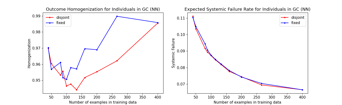
Figure 1: Data sharing leads to more homogeneous outcomes. Data-sharing results for GC using neural network classifiers, which shows homogenization (left) and expected systemic failure rate (right) as a function of training dataset size ($x$-axis).

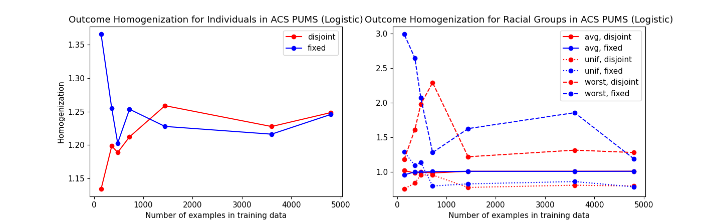
Figure 2: Picking on the same person. Data-sharing results for ACS PUMS using logistic regression: individual-level homogenization (left) exceeds group-level (right; avg and unif).

Results and analysis. We report results in Figure 1 and Figure 2 to demonstrate specific phenomena, deferring the remainder of the results to Appendix C. In Figure 1 (left), we see clear evidence for our hypothesis: the fixed setting, which by construction involves more sharing, reliably shows more homogeneity than the disjoint setting. Overall, across all 3 datasets and 4 model families we consider, we find that the fixed setting generally leads to more homogeneous outcomes than disjoint, which provides evidence towards our hypothesis: the use of the same training data leads to greater outcome homogenization than the use of different (but identically distributed) training data.

However, this relationship is not perfect: we do see several instances where the degree of homogeneity is similar or even sometimes greater for the disjoint setting (e.g. regions of the left subplot of Figure 2). Therefore, data sharing alone does not fully characterize homogeneity (e.g. randomness in training and instability in the number of observed systemic failures are important to consider). Conceptually, we highlight that this is critical to the character of systemic failures: data points that are failed by all models are very sensitive and, as a result, the trends can be quite fickle even in very pure settings with very controlled sharing like the ones we consider here.

Further, the trends in the error rates for fixed and disjoint are near-identical (right subplot of Figure 1), as we would expect given the relationship between the sampling protocols. That is, this is clear evidence of an important qualitative consequence: by looking at accuracy alone, these settings are indistinguishable, whereas they differ considerably in terms of the number of observed systemic failures. Our measures correctly identify discrepancies in these settings, even though the underlying error rates are the same. Finally, as a function of dataset size, we do not see consistent trends on the relationship between dataset scale and outcome homogenization, though we unsurprisingly see the disjoint and fixed settings converge for larger dataset sizes (since the discrepancies in the sampling become negligible due to convergence in measure).

Picking on the same person, not just the same group. For ACS PUMS in Figure 2, we contrast the individual-level and group-level homogenization. (Recall the average and uniform metrics are the group-level analogues of our individual-level metric.) Outcomes are consistently more homogeneous at the individual-level than for racial groups. In fact, group-level analysis shows little homogenization (values near $1$) and little change as a function of dataset size, whereas individual-level measurement exposes greater homogeneity and more variation (which is unsurprising since group-level quantities are more extensively aggregated). This has significant ramifications for many works on algorithmic fairness, which only consider social groups (e.g. race): these works may miss systemic failures for particular individuals that are obscured at the group-level (cf. Kearns et al., 2018; Hashimoto et al., 2018). Even intersectional approaches (Crenshaw, 1989) may not suffice to surface these systemic failures, unless each intersectional "group" reduces to a single individual. As a results, to build comprehensive and holistic accounts of algorithmic harm, we recommend an individual-centric lens as essential complements to widespread group-centric analyses.

5 Model-sharing Experiments

Having found that data sharing appears to exacerbate outcome homogenization, we now turn to model sharing. Specifically, we test how sharing foundation models (FMs) affects outcome homogenization. Bommasani et al. (2021) define foundation models as "models trained on broad data (generally using self-supervision at scale) that can be adapted to a wide range of downstream tasks". FMs have ushered in a sweeping paradigm shift, transforming AI research in many subareas (most notably NLP) and accelerating the productionization process from AI research to AI deployment. Focusing on their concrete societal impact, foundation models are increasingly central to deploying ML at both startups (e.g. Hugging Face, Cohere, AI21 Labs) and established technology companies (e.g. Google, Microsoft, OpenAI).

Sharing is endemic to the FM paradigm: to justify their immense resource requirements, models must be used repeatedly for costs to amortize favorably. In the extreme, if an entire domain like NLP comes to build almost all downstream systems on one or a few FMs, then any biases or idiosyncrasies of these models that pervasively manifest downstream could potentially yield unprecedented systemic failures and outcome homogenization (Bommasani et al., 2021; Fishman and Hancox-Li, 2022). We see initial evidence for such algorithmic monoculture: BERT was downloaded 24 million times in the past month alone and GPT-3 enables hundreds of deployed applications. Consequently, we believe it is especially timely to understand if, and to what extent, outcomes get homogenized as these models become entrenched as infrastructure.

5.1 Experiments

Data. To test how foundation models influence homogenization, we conduct experiments for both vision and language data. On the vision side, we work with the CelebA dataset (Liu et al., 2015) of celebrity faces paired with annotations for facial attributes. For each face image, given the associated attributes, we define two tasks (Earrings, Necklace) that involve predicting whether the individual is wearing the specific apparel item. Attribute prediction in CelebA has been studied previously in work on fairness and robustness (Sagawa* et al., 2020; Khani and Liang, 2021; Wang et al., 2021). On the language side, we use four standard English text classification datasets following Gururangan et al. (2019): IMDB (Maas et al., 2011), AGNews (Zhang et al., 2015), Yahoo (Chang et al., 2008), and HateSpeech18 (de Gibert et al., 2018).

Individuals and groups. Since the vision tasks are all based on CelebA, we have individual-level information. However, since the language tasks involve entirely different data (e.g. movie reviews vs. news articles), there is no (shared) individual-level information. At the group-level, for vision we use annotations for hair color and for whether the individual has a beard, whereas for language we automatically group inputs by binary gender. We deliberately do not use gender or racial information in CelebA because we believe inference of such information from face images is fraught, and has been the subject of extensive critique.

Experimental design. To test if and how model sharing influences outcome homogenization, akin to data sharing, we must precisely specify what it means to share models. In the vision experiments, we produce task-specific models for each task by either (i) training from scratch on CelebA data, (ii) linearly probing by fitting a linear classifier on features from the CLIP foundation model (Radford et al., 2021), or (iii) finetuning CLIP. To ensure meaningful comparisons, the models trained from scratch shared the same ViT architecture (Dosovitskiy et al., 2021) used in CLIP but with weights initialized randomly.

In the language experiments, we further hone in on the specific adaptation method used to adapt the foundation model (specifically RoBERTa-base (Liu et al., 2019)) to each task. We consider (i) linear probing, (ii) finetuning, and (iii) BitFit (Ben Zaken et al., 2022), which is a recent lightweight finetuning method that involves freezing all the FM weights except the bias parameters which are updated as in finetuning. Consequently, BitFit is an intermediary between probing and finetuning, which has been shown to achieve similar accuracy as finetuning while updating very few FM parameters (Ben Zaken et al., 2022). For both vision and for language, all models are trained for the same number of epochs and we repeat each experiment for 5 random seeds per training approach.

Hypotheses. Much like data sharing, model sharing is graded and is not binary: different downstream systems can share varying degrees of underlying models. By design, our experimental design suggests a continuum in sharing: first, downstream system either can share a foundation model or not (scratch). Second, among methods that involve foundation models, all methods initialize the weights using the FM weights but differ in which parameters remain the same after adaptation is completed: finetuning changes all the parameters, BitFit only changes the bias parameters, and probing changes none of the parameters. As a result, overall, we can rank methods from most to least sharing as (i) probing, (ii) BitFit, (iii) finetuning, (iv) scratch, which leads us to predict the amount of homogenization will also follow this ranking under our component-sharing hypothesis.

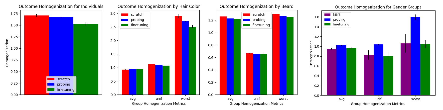
Figure 3: Model-sharing does not reliably lead to more homogeneous outcomes. Model-sharing results as a function of training/adaptation method for vision (left three) and language (rightmost).
Vision: scratch is the most homogeneous, then probing, then finetuning.
Language: probing is the most homogeneous; finetuning and BitFit are similarly homogeneous.

Results and analysis. In Figure 3 (left), across all vision settings, we surprisingly find that scratch is the most homogeneous, i.e. more homogeneous than either approach involving shared FMs. This is the opposite of what we hypothesized: we posit that this may indicate model sharing is not the key explanatory variable for outcome homogenization here, but instead it is a more complex form of data sharing. Specifically, we conjecture that since the scratch models are only trained on CelebA data, whereas the others also are trained on the much larger WebImageText via the CLIP foundation model, this may mean that the models based on CLIP are effectively regularized from learning idiosyncrasies of CelebA that the scratch models acquire. This may more generally suggest that a more correct hypothesis around data sharing should factor in the relationship (e.g. distribution shift) between the training data and the evaluation data for each model. Additionally, we find probing is consistently more homogeneous than finetuning, which aligns with our hypothesis. Finally, akin to the data-sharing experiments (§ 4), we once again find that outcome homogenization is significantly higher for individuals than for groups (comparing to $H_{\textbf{avg}}$ and $H_{\textbf{unif}}$).

In Figure 3 (right), across all language settings, we find the trends in homogenization largely matches what our hypothesis predicts. However, instead of BitFit demonstrating more homogenization than finetuning, we find they are roughly equally homogeneous. In particular, based on shared parameters, the final BitFit models across tasks share $99.92\%$ of the parameters from the FM weight initialization, which is much closer to probing ($100\%$) than to finetuning ($0\%$). That is, while these results agree with our hypothesis (i.e. we see the most homogenization in the probing setting, much like we saw in the vision experiments), the number of shared parameters is probably not the right lens for understanding model sharing. Instead, we may need a more sophisticated account of how the FM weights change due to the adaptation process (cf. Kumar et al., 2022). More broadly, these results do suggest parameter-sharing effects contribute to outcome homogenization within the foundation model regime, but comparisons between foundation models and no foundation models may be more complex to explain.

5.2 Correlations between Metrics

Since we introduce several metrics, we measure the correlations between our metrics. Further, we measure correlations with accuracy (specifically, the expected rate of systemic failure) to test if homogenization is disentangled from accuracy. Since outcome homogenization is related to fairness, we also measure the correlation between our metrics and a standard group fairness metric. Fairness metrics are generally defined for a single model $h$, whereas we study entire systems $\{h^{i}\}_{i=1}^{k}$. We extend the unfairness definition used by Khani et al. (2019) as the variance in the systemic failure rates across groups.

$$\textsc{unfairness}_{G}(h^{1},\dots,h^{k})\triangleq\operatorname*{\text{Var}}\limits_{g}\left[\prod\limits_{i}\textsc{fail}_{g}(h^{i})\right]$$ (6)

	Vision					Language
	$H_{\textbf{avg}}$	$H_{\textbf{unif}}$	$H_{\textbf{worst}}$	Accuracy	Unfairness	$H_{\textbf{avg}}$	$H_{\textbf{unif}}$	$H_{\textbf{worst}}$	Accuracy	Unfairness
$H_{\textbf{avg}}$	-	(0.87, 0.93)	(0.0, 0.96)	(0.0, 0.09*)	(0.0, 0.8)	-	(0.22, -0.47)	(0.11, 0.56)	(0.06*, -0.22*)	(0.02, 0.09)
$H_{\textbf{unif}}$	(0.87, 0.93)	-	(0.0, 0.96)	(0.0, -0.02)	(0.0, 0.74)	(0.22, -0.47)	-	(0.63, -0.53)	(0.0, 0.19*)	(0.0, -0.01)
$H_{\textbf{worst}}$	(0.0, 0.96)	(0.0, 0.96)	-	(0.05, 0.1*)	(1.0, 0.82)	(0.11, 0.56)	(0.63, -0.53)	-	(0.02, 0.13)	(0.13, 0.47)

Table 1: Inter-metric correlations. Correlations amidst our metrics as well as with other metrics reported as (Pearson $R^{2}$, Spearman $\rho$) with * significant at $p=0.05$ and italics significant at $p=0.001$.

Results. In Table 1, we report the pairwise correlation between metric pairs, based on the models we trained in § 5.1. These correlations are for 45 systems (3 methods $\times$ 3 groupings $\times$ 5 random seeds) of 2 models for vision and 15 systems of 4 models for language. For vision, our metrics are highly correlated with each other, whereas for language, $H_{\textbf{unif}}$ patterns quite differently (columns 1-3, 6-8). Since the group-level metrics differ in how they weigh groups, we find this result is largely predictable: for the vision data, groups (e.g. hair colors) all share similar frequencies, whereas the female group is significantly rarer than the male group in the language datasets. For both language and vision, we find that our metrics are generally not correlated, or perhaps weakly correlated, with accuracy/error as we intended (columns 4, 9). With respect to fairness, our worst-case metric $H_{\textbf{worst}}$ is strongly correlated for both modalities, but for the other two metrics we see no linear correlations and only monotone correlations for the vision experiments (columns 5, 10). This is in line with our broader expectations that (system-level) fairness and outcome homogenization are indeed related (especially for the worst-performing group), but that given they are distinct theoretical constructs, they should not always be correlated (Campbell and Fiske, 1959).

5.3 Discussion

Across our experiments, we provide considerable evidence that sharing leads to homogeneous outcomes, but that it is incomplete explanation of homogeneity. This is particularly relevant when the findings in § 4 and § 5 are contrasted, given model sharing in the foundation model regime indirectly implies immense data sharing via the training data (as mediated by the FM weight initialization). We emphasize that the regimes for these findings are quite different: low-dimensional tabular data with simple model families in our data-sharing experiments vs. high-dimensional images/text with large neural networks in our model-sharing experiments, so discrepancies in the findings may be attributable to these differences. More broadly, we believe a more complete explanation requires accounting for the data distributions and the associated distribution shifts (e.g. between training and adaptation) at play. What we believe is clear, however, is that our findings provide an empirical basis to build on our conceptual arguments that sharing in machine learning can increase homogenization. This motivates investigation into real deployments of machine learning: for example, does sharing/monoculture lead to homogenization in algorithmic hiring?

6 Societal Considerations

To situate our work in a broader social context, we articulate how we reason about the harms of outcome homogenization as well as identify core challenges to diagnosing, measuring, and rectifying outcome homogenization in real deployed systems.

6.1 Why are Homogeneous Outcomes Harmful?

To this point, we have argued homogeneous outcomes are a class of systemic harms and, in particular, a class of harms we should be paying greater attention to given pervasive practices of sharing and monoculture. In some settings, it may feel clear that homogeneous outcomes are harmful: we surely do not want individuals to be failed by every classifier they interact with and it is at least possible for the classifiers to correctly classify the individual. In others, such as our motivating example of hiring, it may feel less clear. Surely there is harm if someone is locked out from employment across all employers, especially if this lockout can be traced to a shared algorithm being deployed by each employer? On the other hand, some people must be rejected from every employer (in the absence of broader structural change) if the total number of candidates exceeds the number of open positions, and there may be justifiable circumstances to reject someone from all positions even when there are unfilled vacancies.

Overall, understanding when homogeneous outcomes constitute a social harm is contextual: the particular circumstances determine how to interpret whether, and to what extent, homogenization is of moral concern. To provide one account of how to reason about these harms, we follow Elizabeth Anderson in taking a relational egalitarian approach (Anderson, 1999, 2016) to evaluate the social harm of homogenization. Relational egalitarianism, as a theory of justice, argues that individuals must relate to each other as equals in a just society. Relational approaches have seen recent adoption in relation to AI: Birhane (2021) presents a relational account of algorithmic injustice with similar approaches taken to data governance, decision-making, and fairness (Viljoen, 2021; Kasy and Abebe, 2021; Fish and Stark, 2022).

To ground a relational analysis, we return to the context of hiring. While individual organizations may establish rankings of candidates, and indeed we would expect that companies within a market sector will often agree on a hierarchy, the same hierarchy should not consistently dominate an entire sector or territory such that some people are entirely excluded from work (Anderson, 1999, 74). Anderson argues that “to be capable of functioning as an equal participant in a system of cooperative production requires …access to the education needed to develop one’s talents, freedom of occupational choice, the right to make contracts and enter into cooperative agreements with others, the right to receive fair value for one’s labor, and recognition by others of one’s productive contributions” (Anderson, 2016, 318). If some people are consistently excluded from job interviews and, therefore, employment, they will not enjoy freedom of occupational choice; if they are excluded from higher education, they will struggle to develop their talents. Not only do those excluded personally suffer from the establishment of the hierarchy, they also are unable to function as equal participants in society. Because employment, education, and credit are foundational social goods, consistent exclusion from them risks establishing a social hierarchy of esteem or domination. The hierarchy of esteem in turn damages the ability of the excluded to relate to others as equal democratic citizens (Anderson, 1999).

Under this account, we emphasize how the moral importance of the harm depends on the scale of exclusion. That is, in its purest form, there is a strong threshold effect: homogeneous outcomes are most severe when the individual is denied from all sources of employment (or education or credit or so on). If autonomy is access to a sufficient range of sufficiently varied opportunities, then it is not a harm to be denied one opportunity, such as a job or a loan (Raz, 1988). It is a harm, however, to be shut out of all opportunities. For this reason, in this work, we study the extreme case in which individuals are shut out of all opportunities.

6.2 Practical Challenges for Outcome Homogenization

Diagnosis. In our work, we posit monoculture yields homogenization: to follow this approach would require knowing which deployments rely on the same vendor, dataset, or foundation model (i.e. knowing where there is monoculture). Unfortunately, how algorithmic systems are constructed is often so opaque that identifying shared components is nigh impossible. However, if high homogenization were demonstrated, the measurement itself could justify provisions for increased transparency to identify the latent monoculture (i.e. the anti-causal direction). This provides a plausible mechanism for empowering auditors to be granted conditional access to otherwise inaccessible proprietary systems.

Measurement. Measuring homogenization only requires black box access, which is often achievable in practice (see Buolamwini and Gebru, 2018; Raji and Buolamwini, 2019; Metaxa et al., 2021). However, identifying individual-level effects requires linking individual outcomes across deployments. Due to privacy constraints, linking individuals across different deployments may be challenging or impossible, which motivates group-level homogenization as more generally accessible (see § 3.2).

Rectification. Even once outcome homogenization is identified, organizations may not be incentivized to reduce it. In fact, homogenization neither is attributable to any single entity nor can it always be addressed by unilateral action from a single organization. In the face of misaligned incentives and collective action problems, regulation, policy, or other compliance mechanisms may be required. Potential trade-offs between organization incentives and homogenization are further complicated if the harms of homogeneous outcomes take time to observe/accrue, but the benefits of, say, maximizing accuracy are immediate. More optimistically, Kleinberg and Raghavan (2021) show (under specific conditions) no trade-off exists between accuracy-maximizing policies and diversifying outcomes for societal benefit.

7 Limitations and Conclusion

We have introduced, formalized, and measured outcome homogenization as a systemic harm that may arise from practices of sharing in ML. Outcome homogenization is a new, understudied, and conceptually compelling topic: its definition, interpretation, statistical estimation, mitigation, and connections to monoculture remain poorly understood in spite of this work. We encourage future work to push in all of these directions. As to our measure, direct optimization may not lead to desirable outcomes, potentially even contributing to ethics-washing: its interpretation must be contextual since the implications of homogeneous outcomes heavily depend on broader societal context.

We believe homogenization is essential to holistically characterizing algorithmic harm, especially given growing monoculture (e.g. via foundation models). Without scrutiny, its harms may insidiously entrench. Consequently, we believe early intervention is necessary to prevent such harms in society.

Reproducibility.

All code, data, and experiments are available on GitHub and CodaLab Worksheets.

Checklist

1. For all authors…

   1. Do the main claims made in the abstract and introduction accurately reflect the paper’s contributions and scope? [Yes] See metrics section (§ 3) and experimental sections (§ 4, § 5).

   2. Did you describe the limitations of your work? [Yes] See metrics section (§ 3), societal considerations (§ 6), and conclusion (§ 7).

   3. Did you discuss any potential negative societal impacts of your work? [Yes] See societal considerations (§ 6) and conclusion (§ 7).

   4. Have you read the ethics review guidelines and ensured that your paper conforms to them? [Yes]

2. If you are including theoretical results…

   1. Did you state the full set of assumptions of all theoretical results? [N/A]

   2. Did you include complete proofs of all theoretical results? [N/A]

3. If you ran experiments…

   1. Did you include the code, data, and instructions needed to reproduce the main experimental results (either in the supplemental material or as a URL)? [Yes] See https://worksheets.codalab.org/worksheets/0x807c29f8eb574d1fba8f429ec78b5d1b and Appendix B.

   2. Did you specify all the training details (e.g., data splits, hyperparameters, how they were chosen)? [Yes] See Appendix B.

   3. Did you report error bars (e.g., with respect to the random seed after running experiments multiple times)? [Yes] See Figure 3.

   4. Did you include the total amount of compute and the type of resources used (e.g., type of GPUs, internal cluster, or cloud provider)? [Yes] See Appendix B.

4. If you are using existing assets (e.g., code, data, models) or curating/releasing new assets…

   1. If your work uses existing assets, did you cite the creators? [Yes] See § 4, § 5, and Appendix B.

   2. Did you mention the license of the assets? [No] We provide references directly to where we sourced data in Appendix B.

   3. Did you include any new assets either in the supplemental material or as a URL? [N/A]

   4. Did you discuss whether and how consent was obtained from people whose data you’re using/curating? [No] We defer to the discussions in prior work, though we did check ourselves for any specific concerns of consent and found none in our initial cursory investigation.

   5. Did you discuss whether the data you are using/curating contains personally identifiable information or offensive content? [Yes] Yes, some of our data contains PII (e.g. Census information, face images) and one of our datasets is related to hate speech detection, so this is by design. These are well-established datasets, with the respective works providing discussion on these fronts, and we do not foresee any specific harms from our usage.

5. If you used crowdsourcing or conducted research with human subjects…

   1. Did you include the full text of instructions given to participants and screenshots, if applicable? [N/A]

   2. Did you describe any potential participant risks, with links to Institutional Review Board (IRB) approvals, if applicable? [N/A]

   3. Did you include the estimated hourly wage paid to participants and the total amount spent on participant compensation? [N/A]

Appendix A Homogenization Metrics

A.1 Group Homogenization Metrics

In § 3.2, we introduced our group level homogenization metrics. Specifically, we note the design decision of how to weight groups and the three weightings we consider: average, uniform, and worst. Here, we provide the full mathematical definition of these metrics.

For convenience, let the frequency of group $g$ in a specific dataset $D^{i}$ by denoted as $p^{i}(g)$, and the joint probability of the group across all datasets be denoted as $p(g)\triangleq\prod_{i=1}^{k}p^{i}(g)$.

$$\text{$H_{\textbf{avg}}$}(h^{1},\dots,h^{k}) \triangleq\frac{\sum\limits_{g}\left[\frac{p(g)}{\sum_{g^{\prime}}p(g^{\prime})}\prod\limits_{i}\textsc{fail}_{g}(h^{i})\right]}{\prod\limits_{i}\textsc{fail}(h^{i})}$$ (7)

$$\text{$H_{\textbf{unif}}$}(h^{1},\dots,h^{k}) \triangleq\frac{\mathop{\mathbb{E}}\limits_{g}\left[\prod\limits_{i}\textsc{fail}_{g}(h^{i})\right]}{\prod\limits_{i}\textsc{fail}(h^{i})}$$ (8)

$$\text{$H_{\textbf{worst}}$}(h^{1},\dots,h^{k}) \triangleq\frac{\max\limits_{g}\left[\prod\limits_{i}\textsc{fail}_{g}(h^{i})\right]}{\prod\limits_{i}\textsc{fail}(h^{i})}$$ (9)

A.2 Relating Individual and Group Homogenization

In § 4, we demonstrate empirically that outcomes can be more homogeneous for individuals than for racial groups. One may be led to believe that homogenization is necessarily greater when considering finer-grained groupings since individuals (when viewed as singleton groups) are subsets of groups (i.e. when grouping by individuals, no data points from different races appear in the same group as each group is a singleton). However, this is not true.

To elucidate this, we provide two toy scenarios that demonstrate circumstances where individual-level outcome homogenization is greater than, and is less than, group-level outcome homogenization. (Of course, they can also be equal.) In both settings, we will have two models (i.e. two decision-makers) and two groups, where each group is comprised of two individuals. As a result, $H_{\textbf{avg}}$= $H_{\textbf{unif}}$, so we can compare either to $H^{\textbf{individual}}$.

In both settings, we will say Alice and Angelique are members of Group 1 and Bob and Bernardo are members of Group 2.

Scenario 1. Let Alice and Bob be misclassified by $h^{1}$ but correctly classified by $h^{2}$. Let Angelique and Bernardo be misclassified by $h^{2}$ but correctly classified by $h^{1}$. No one is misclassified by both models, hence the number of observed systemic failures is 0 at the individual level, hence $H^{\textbf{individual}}$= 0.

However, since there is a failure within Group 1 for both models (and for Group 2 as well), the number of systemic failures is nonzero at the group level, hence $\text{$H_{\textbf{avg}}$}~{}=~{}\text{$H_{\textbf{unif}}$}~{}>0$. Thus, in this scenario, we have seen that individual-level outcome homogenization can be less than group-level outcome homogenization.

Scenario 2. Let Alice and Bob be misclassified by both $h^{1}$ and $h^{2}$. Let Angelique and Bernardo be correctly classified by both $h^{1}$ and $h^{2}$. At the individual level, there are 2 observed systemic failures, so the observed rate of systemic failure is $\frac{2}{4}=0.5$. The overall error rate for each application is 0.5, so the expected rate of systemic failure is $0.5\times 0.5=0.25$. Therefore, $H^{\textbf{individual}}$= $\frac{0.5}{0.25}=2$.

At the group level, the rate of systemic failures is $0.25$ for both groups. The overall error rate for each application is still 0.5, so the denominator is also $0.5\times 0.5=0.25$. Therefore, $\text{$H_{\textbf{avg}}$}=\text{$H_{\textbf{unif}}$}=\text{$H_{\textbf{worst}}$}=1$. Thus, in this scenario, we have seen that individual-level outcome homogenization can be greater than group-level outcome homogenization.

A.3 Generalizing Individual-Level Metric

In § 3.3, we note that our individual-level framing assumes that every individual $j$ produces inputs $x_{j}^{i}$ for every decision-maker $i$. The formalism in the main paper already permits these inputs to be different across decision-makers for the same individual (e.g. Bob may submit different resumes when applying to Microsoft and Google). However, the formalism does not support two further general concepts: (i) multiple inputs per decision-maker and (ii) no inputs for some decision-maker (e.g. Bob does not apply to Amazon). To accommodate the former, we note that the notion of failure can be modified depending on how the outcomes for the multiple inputs should be aggregated (e.g. a failure of a search engine may be determined by some fraction of search queries producing poor results for the user).

To address the latter concern, we introduce notation $c_{j}$ to indicate the subset of decision-makers that individual $j$ interacts with, i.e. $c_{j}\subseteq\{1,\dots,k\}$. That is, any decision-makers $i\in\{1,\dots,k\}$ that are not in $c_{j}$ are those that individual $j$ does not interact with. Accordingly, we definite $H^{\textbf{individual}}$ as:

$$\text{$H^{\textbf{individual}}$}(h^{1},\dots,h^{k})\triangleq\frac{\mathop{\mathbb{E}}\limits_{j}\left[\prod\limits_{i\in c_{j}}F^{i}(x_{j}^{i})\right]}{\mathop{\mathbb{E}}\limits_{j}\left[\prod\limits_{i\in c_{j}}\textsc{fail}(h^{i})\right]}$$ (10)

Notably, when $\forall j,~{}c_{j}=[k]$, the denominator simplifies to $\prod\limits_{i\in[k]}\textsc{fail}(h^{i})$, which matches Equation 3.

A.4 Alternative Metrics

In § 3, we introduce the metrics we use to quantify outcome homogenization. Of course, much like the many mathematical expressions that have been used to measure bias and fairness, there are many ways to reasonably measure homogenization. Fundamentally, given the underlying construct of outcome homogenization is largely new, we begin by recognizing our understanding of the concept is incomplete and likely will require study in real systems to truly identify the precise desiderata for a measure.

In the interim, it is difficult to assess if the metric has structural fidelity [Loevinger, 1957], i.e. does the metric’s structure faithfully captures outcome homogenization? Further, it is unclear if the metric has sufficient predictive validity to predict long-term outcomes (e.g. longitudinal harms arising from outcome homogenization) or how useful it is for testing specific scientific and social hypotheses [Jacobs and Wallach, 2021]. Ultimately, we believe the key test for the metric will be its consequential validity [Messick, 1987]: will the metric yield positive social impact as it "both reflects structure in the world and imposes structure upon the world" [Hand, 2016].

To facilitate understanding, we transparently discuss other metrics we considered and why they may be preferable in some circumstances. Ultimately, we worked with the metrics we describe in the paper as we found them to be the simplest and preferred their probabilistic interpretations, but we include reasons to prefer alternatives as we describe them.

A.4.1 Alternative Metrics in the Binary Setting

Covariance and Pointwise Mutual Information. When $k=2$, i.e. there are two decision-makers, we note that our metric bears a very close resemblance to the covariance between the (indicator) random variables $F^{1}$ and $F^{2}$. In particular, the covariance is the difference of the quantities that define the ratio for our homogenization metric. Similarly, our metric is the pointwise mutual information (PMI) evaluated at $(1,1)$ up to the $\log$.

$$\text{$H^{\textbf{individual}}$}(h^{1},h^{2}) =\frac{\mathop{\mathbb{E}}\limits_{j}\big{[}F^{1}F^{2}\big{]}}{\mathop{\mathbb{E}}\limits_{j}\left[F^{1}\right]\mathop{\mathbb{E}}\limits_{j}\left[F^{2}\right]}$$ (11)

$$\text{Cov}(F^{1},F^{2}) =\mathop{\mathbb{E}}\limits_{j}\big{[}F^{1}F^{2}\big{]}-\mathop{\mathbb{E}}\limits_{j}\left[F^{1}\right]\mathop{\mathbb{E}}\limits_{j}\left[F^{2}\right]$$ (12)

$$\text{PMI}(F^{1}=1,F^{2}=1) =\log\left(\frac{\mathop{\mathbb{E}}\limits_{j}\big{[}F^{1}F^{2}\big{]}}{\mathop{\mathbb{E}}\limits_{j}\left[F^{1}\right]\mathop{\mathbb{E}}\limits_{j}\left[F^{2}\right]}\right)=\log\left(\text{$H^{\textbf{individual}}$}(h^{1},h^{2})\right)$$ (13)

With respect to the covariance, we prefer that our metric is more naturally comparable across settings where the failure rates of social systems vary, whereas the covariance is more directly tied to the absolute scale of the failure rates. With respect to the pointwise mutual information, we note that we are simply looking at the behavior of the social system in a special case where all models fail (which is one of the $2^{k}$ possible outcomes an individual could receive overall), whereas the overall PMI considers all of them and is invariant to symmetries that are significant in our setting. Further, both are traditionally studied in the binary setting, whereas we study behavior in settings where $k>2$.

Pearson Correlation. Building on the relationship with the covariance, we note that our metric therefore also resembles the Pearson correlation.

$$\text{$H^{\textbf{individual}}$}(h^{1},h^{2}) =\frac{\mathop{\mathbb{E}}\big{[}F^{1}F^{2}\big{]}}{\mathop{\mathbb{E}}\left[F^{1}\right]\mathop{\mathbb{E}}\left[F^{2}\right]}$$ (14)

$$\text{Corr}(F^{1},F^{2}) =\frac{\mathop{\mathbb{E}}\big{[}F^{1}F^{2}\big{]}-\mathop{\mathbb{E}}\left[F^{1}\right]\mathop{\mathbb{E}}\left[F^{2}\right]}{\sqrt{\left(\mathop{\mathbb{E}}\left[F^{1}\right](1-\mathop{\mathbb{E}}\left[F^{1}\right])\right)\left(\mathop{\mathbb{E}}\left[F^{2}\right](1-\mathop{\mathbb{E}}\left[F^{2}\right])\right)}}$$ (15)

In particular, when dealing with accurate models that are homogeneous (i.e.  $\mathop{\mathbb{E}}\big{[}F^{1}F^{2}\big{]}>>\mathop{\mathbb{E}}\left[F^{1}\right]\mathop{\mathbb{E}}\left[F^{2}\right]$), the Pearson correlation coefficient approximates our metric up to the square root in the denominator. Arguments can be made in favor and against this square root (and more generally a $k$-th root for $k>2$); for simplicity we favor our metric that does not introduce such normalization but acknowledge this normalization may prove to be more favorable as the metric is further stress-tested.

A.4.2 Alternative Metrics beyond the Binary Setting

As we note in Footnote 2, our formalism and metrics are designed to be general, meaning that they can accommodate settings where the models $h^{i}$ correspond to different tasks or scenarios. (We make use of this generality in our experiments (§ 5) for vision and, especially, language.) To permit this generality, we (reductively) binarize outcomes as either failures or not in our use of the indicator functions $F^{i}$. In particular, for arbitrarily different tasks, the outcome spaces and their consequences on individuals may not be (easily) related.

In some settings, specifically those where the tasks that constitute the social system are sufficiently similar, we may instead prefer a more graded loss in the place of the binary notion of failures. For each deployment by decision-maker $i$, denote the associated loss function as $\mathcal{L}^{i}$ such that $\mathcal{L}^{i}(h^{i}(x_{j}^{i}),y_{j}^{i})=\ell_{j}^{i}$ is the loss experienced by individual $j$ when interacting with model $h^{i}$. In these settings, where the loss achieved across different applications is comparable, we can consider additional measures for homogenization in terms of this loss.

$$\text{$H^{\textbf{individual}}$}(h^{1},\dots,h^{k}) =\frac{\mathop{\mathbb{E}}\limits_{j}\left[\prod\limits_{i}~{}\ell_{j}^{i}\right]}{\prod\limits_{i}\left[\mathop{\mathbb{E}}\limits_{j}~{}\ell_{j}^{i}\right]}$$ (16)

$$\text{MinExp}(h^{1},\dots,h^{k}) =\frac{\mathop{\mathbb{E}}\limits_{j}\left[\min\limits_{i}~{}\ell_{j}^{i}\right]}{\min\limits_{i}\left[\mathop{\mathbb{E}}\limits_{j}~{}\ell_{j}^{i}\right]}$$ (17)

$$\text{ExpExp}(h^{1},\dots,h^{k}) =\frac{\mathop{\mathbb{E}}\limits_{j}\left[\min\limits_{i}~{}\ell_{j}^{i}\right]}{\mathop{\mathbb{E}}\limits_{i}\left[\mathop{\mathbb{E}}\limits_{j}~{}\ell_{j}^{i}\right]}$$ (18)

In words, the MinExp definition is the ratio of the average best-case loss for individuals with the loss of the best model $h^{\text{best}}$ and the ExpExp definition is the same but the denominator is the average loss of the models rather than the best loss. These definitions bear close resemblance to the MaxMin and lexicographic (leximax and leximin) fairness definitions studied in the fairness literature [Dubins and Spanier, 1961, Henzinger et al., 2022]; the group-weighted analogue that use the worst group weighting recovers the MaxMin definition in the denominator. (Note that the naming conventions are reversed since we define metrics in terms of loss whereas work in fairness and equitable allocations generally defines metrics in terms of utility.)

When the loss is the 0-1 classification loss, the MinExp definition and $H^{\textbf{individual}}$  are very similar: the numerators are the same (as the product of indicator variables is the same as their minimum) and the denominators are precisely $z=\frac{\prod_{i=1}^{k}\textsc{fail}(h^{i})}{\textsc{fail}(h^{\text{best}})}$ factors of each other (i.e. the failure rate of all of the models except the best one). Consequently, the MinExp yields values in the range $[0,1]$ whereas $H^{\textbf{individual}}$ is in $[0,\infty)$. Independent behavior across models in $H^{\textbf{individual}}$ is guaranteed to be 1 and maximal systemic failure in MinExp is guaranteed to be 1; symmetrically, independent behavior in MinExp is $z$ (which is non-constant) and maximal systemic failure in $H^{\textbf{individual}}$ is $\frac{1}{z}$.

More broadly, the indicator variables we use in the main paper can be seen as a special case when using the 0-1 classification loss whereas arbitrary loss functions can be mapped to indicators by thresholding the loss (which does not require the loss to comparable, as different thresholds can be applied for different deployments). As a result, both $H^{\textbf{individual}}$ and MinExp have clear merits; we believe MinExp may especially be a more natural definition where individuals have choices on which model $h^{i}$ to interact with of the $k$ possible models. In these settings (e.g. picking which voice assistant to use, or more generally consumer products), the losses will naturally be comparable and it may suffice for the individual to have one good option, which is more smoothly encoded by the minimum of the loss rather than the product of the indicators.

We encourage future work to explore whether the MinExp or $H^{\textbf{individual}}$ is preferable: in many settings we expect they will be strongly correlated given they are scalings of each other that depend not on the correlated nature of errors but the overall error rates, but they may be some settings where they diverge and one is clearly preferable to the other. Currently, we recommend work to also consider MinExp when the losses are comparable, but to default to $H^{\textbf{individual}}$ since this is not required and $H^{\textbf{individual}}$ has a simple probabilistic interpretation.

Appendix B Reproducibility

All code, data, and experiments are available on GitHub and CodaLab Worksheets. We provide further experimental details below.

B.1 Census Experiments

B.1.1 Data

We work with the ACS PUMS data introduced by Ding et al. [2021], which contains US Census survey data for 3.6 million individuals. Ding et al. [2021] introduce the dataset to facilitate research into algorithmic fairness and the measurement of harms associated with algorithmic systems. For each individual in the Census, 286 features are recorded (e.g. self-reported race and sex, occupation, average hours worked per week, marital status, healthcare status). Ding et al. [2021] construct several classification tasks using this data, where each task uses some of an individual’s features as inputs and one of their features as the label for the prediction task (e.g. predicting if an individual’s income exceeds $50000). Of these tasks, we work with three in particular: ACSEmployment (predict if an individual is employed), ACSIncomePovertyRatio (predict an individual’s income normalized by the poverty threshold), and ACSHealthInsurance (predict if an individual has health insurance). Following Ding et al. [2021], we split the data 80/20 for train/test. We access this data through their folktables package. We use the data for all of the US (they provided state-level data as well) from 2018, which is the primary data they analyze in their paper. We select these tasks because Ding et al. [2021] do not impose any filtering constraints in selecting data for these tasks, meaning all three tasks are posed for the same underlying individuals. See Ding et al. [2021] for more details. License information is provided at https://github.com/zykls/folktables#license-and-terms-of-use and our use of the dataset adheres to these terms of service. The data clearly can be personally identifying given it has census records for particular individuals, but there is no offensive content.

B.1.2 Models

Following Ding et al. [2021], we train logistic regression models using sk-learn [Pedregosa et al., 2011] with default hyperparameters. As a sanity check, we compared average model performance and saw it matched/exceeded what is reported in Ding et al. [2021]. For each setting (fixed, disjoint) and amount of training data, we trained 25 models across 5 random subsamples of training and 5 random seeds for model run per subsample, for each of the three tasks. In aggregate, all of the models we trained took approximately 10 hours across 5 NVIDIA Titan Xp GPUs (or 50 hours on 1 NVIDIA Titan Xp GPU), with additional experiments/debugging that is unreported in the paper taking approximately an additional 400 NVIDIA Titan Xp GPU hours.

B.1.3 Groupings

We consider racial groups, which are already provided in the dataset based on the self-identified category individuals chose in providing their information to the US Census. The specific racial categories used are: White alone, Black/African American alone, American Indian alone, Alaska Native alone, American Indian and Alaska Native, Asian alone, Native Hawaiian and Other Pacific Islander alone, other unspecified race, two or more races.

B.2 Vision Experiments

B.2.1 Data

We work with the CelebA dataset [Liu et al., 2015], which is a widely used dataset of celebrity faces paired with annotations for facial attributes. For each face image, given the associated attributes, we define two tasks (Earrings, Necklace) that involve predicting whether the individual is wearing the specific apparel item. Attribute prediction in CelebA has been studied previously in work on fairness and robustness [Sagawa* et al., 2020, Khani and Liang, 2021, Wang et al., 2021]. Given recent documentation of significant issues with computer vision datasets [e.g.  Birhane and Prabhu, 2021, Birhane et al., 2021], we emphasize that we use the dataset solely for analytic reasons to study homogenization. Further, given works like GenderShades [Buolamwini and Gebru, 2018] that highlight the harms of face recognition, we emphasize that we do not use the dataset for face recognition, but instead consider apparel prediction tasks where each apparel item/accessory is clearly observable in the face image. In addition to Earrings and Necklace, the dataset also contains attributes for Eyeglasses and Neckties. We initially included these tasks, but observed no individual was misclassified for all four tasks since these two tasks were very easy and models rarely produced any errors (e.g. the error rate for Eyeglasses was generally less than $1\%$). To be able to present non-trivial results for individual-level outcome homogenization, we therefore removed these tasks from consideration so that a nonzero number of systemic failures could be observed. We downloaded the CelebA data from https://mmlab.ie.cuhk.edu.hk/projects/CelebA.html. We resized images to 224-by-224, and then apply the same augmentations as in CLIP [Radford et al., 2021], before feeding the image into the ViT-B/16 (which is what Radford et al. [2021] do as well). License information is provided here: https://mmlab.ie.cuhk.edu.hk/projects/CelebA.html. Our use of the dataset is consistent with the requirements for non-commercial research use. The data clearly can be personally identifying given it has face images for particular individuals, but there is no offensive content.

B.2.2 Models

Following Radford et al. [2021], we either use their released 150M parameter ViT-B/16 CLIP model (the largest publicly available CLIP model at the time of writing) or a randomly initialized model with the same architecture. We used code from the official CLIP repository at https://github.com/openai/CLIP. Since Radford et al. [2021] modify the standard Vision Transformer [Dosovitskiy et al., 2021], we use their modified version for our scratch models. As a sanity check of our implementation, we confirmed that our average finetuning accuracy were comparable to prior work (Sagawa* et al. [2020] paper considers the task of predicting Blonde hair, with an ImageNet pretrained ResNet-50, they get 94.8% and we get 95.9% in this particular task, i.e. when we also do the task of predicting Blonde hair with the same ImageNet pretrained ResNet-50). Further, on the Wearing Earrings task, we also confirmed that the CLIP pretrained ViT-B/16 did better than a ResNet-50 (both ImageNet pretrained and CLIP pretrained). For each setting (scratch, probing, finetuning), we trained 5 model runs with different seeds, for each of the tasks. The final learning rates we used were 0.003 (training from scratch), 0.01 (linear probing), 0.000003 (fine-tuning), and they were selected by grid searching the learning rates on the Earrings task and we sanity checked that choosing a higher or lower learning rate led to lower accuracy. We also train each approach for 10 epochs to ensure similar computational resources are provided to each approach. In aggregate, all of the models we trained took approximately 1000 hours on one NVIDIA Titan Xp GPU.

B.2.3 Groupings

We consider groups based on hair color. The dataset provides five hair-related annotations of Black, Brown, Blonde, Grey, and Bald. Since the Bald category was quite small, we collapsed the category with all examples that lacked a hair annotation (e.g. the hair color is obscured due to a hat) into an "Other" category to yield five total categories. In addition, we measure outcome homogenization for individuals based on whether they have a beard. While the CelebA dataset also contains annotations for race and gender, we chose to not look at these groups given we were concerned that the gender/race was being inferred by an annotator (crowdworker) from the face rather than being self-identified [Liu et al., 2015].

B.3 Language Experiments

B.3.1 Data

We use the IMDB, AGNews, Yahoo, and HateSpeech18 datasets. For IMDB, we were unable to find formal license information. The data may contain some PII, but it is unlikely there is significant offensive content. For AGNews, we were unable to find formal license information but found information indicating it should be used non-commercially, which we adhere to see. The data may contain some PII, but it is unlikely there is significant offensive content. For Yahoo, we were unable to find formal license information. The data may contain some PII, especially given its nature, but it is unlikely there is significant offensive content. For HateSpeech18, we adhere to the license provided here: https://github.com/Vicomtech/hate-speech-dataset#license. The data likely contains some PII given it is from forums, and certainly contains offensive content. We access this data through Hugging Face Datasets [Lhoest et al., 2021]. The associated papers describe how the data was collected or scraped. We tokenize the data using the RoBERTa [Liu et al., 2019] tokenizer provided in Hugging Face Transformers [Wolf et al., 2020].

B.3.2 Models

For all models we produced, we adapt RoBERTa-base [Liu et al., 2019] using the weights provided through Hugging Face Transformers [Wolf et al., 2020]. For all models, we use the default hyperparameters in the Trainer provide in the Transformer library, with the only change being a fairly standard setting of the learning rate to 2e-5. As a sanity check of our implementation, we confirmed that our accuracy matches those provided in standard scripts/tutorials provided in Transformers and are quite similar to other works that work with these standard datasets [e.g.  Gururangan et al., 2019]. For each setting (probing, finetuning, BitFit), we trained 5 model runs with different seeds, for each of the four tasks. In aggregate, all of the models we discuss in the paper took approximately 36 hours across 5 NVIDIA Titan Xp GPUs (or 180 hours on 1 NVIDIA Titan Xp GPU), with additional experiments/debugging that is unreported in the paper taking approximately an additional 2000 NVIDIA Titan Xp GPU hours.

B.3.3 Groupings

Since we consider four deployments that are largely unrelated to each other, there are no annotations of individuals or groups available that apply across all four datasets. Consequently, we group inputs by (binary) gender, as this grouping applies across the four datasets. Specifically, for each input we identify whether the input contains more references to the female gender (e.g. uses of words like "she"), the male gender, or no reference to an explicitly gendered term is made. We acknowledge that this treats gender as a binary as part of an unfortunate trend in NLP of works involving gender using binaries [Cao and Daumé III, 2020]. We use the peer-reviewed list of gender terms from Garg et al. [2018] and in accordance with the recommendations of Antoniak and Mimno [2021]. In the event that the same number of male and female gender terms are mentioned (possibly zero for both) in an input, we grouped the input in a third "Other" category. While we did not extensively test, we did observe that the findings were not sensitive to small perturbations (i.e. random deletions of words from each list) of the lists we used.
Following Antoniak and Mimno [2021], we provide the exact lists below.

Male words = {"he", "son", "his", "him", "father", "man", "boy", "himself", "male", "brother", "sons", "fathers", "men", "boys", "males", "brothers", "uncle", "uncles", "nephew", "nephews"}
Female words = {"she", "daughter", "hers", "her", "mother", "woman", "girl", "herself", "female", "sister", "daughters", "mothers", "women", "girls", "femen", "sisters", "aunt", "aunts", "niece", "nieces"}

Appendix C Additional Experiments

Summary.

In § 4, we report results on the ACS PUMS dataset. Here, we supplement those findings to clarify whether the findings generalize across model families and to other datasets. Qualitatively, across these additional evaluations, we do find the findings transfer: (i) the fixed partition of the data, where there is strictly greater data-sharing, reliably yields greater homogenization and (ii) when group-level data is available, individual-level homogenization exceeds group-level homogenization in magnitude.

Datasets.

In § 4, we report results on the ACS PUMS dataset. Here, we replicate the experiments performed in that section, but vary the dataset to clarify if the qualitative trends generalize to other datasets. Recall that the structure of the data we deal with is fairly unusual: we are interested in datasets where each input is associated with multiple outcomes (i.e. the traditional multi-task learning setting) as we will share the training data across the models for each task. However, because of our interests in social outcomes, we would further like each input to be meaningfully associated with a person (e.g. arbitrary multi-task learning datasets could be used but are unideal if they don’t additionally have this human-centric structure).

To identify additional relevant datasets, we survey datasets for multi-task learning, datasets for fairness in ML (which are generally human-centric as desired), and work at the intersection of fairness and multi-task ML. Of these, we looked at Zhang and Yang [2017] for multi-task learning as well as https://paperswithcode.com/task/multi-task-learning, which provided a list of 51 datasets. We also looked at the 15 fairness datasets surveyed by Le Quy et al. [2022]. Finally, Wang et al. [2021] initiated the study of multi-task fairness, considering four datasets.

From all of these, we arrived at four datasets with the structure we wanted: CelebA, UCI Adult, LSAC [Wightman et al., 1998], and GC [German Contracts; Dua and Graff, 2017]. All of these datasets have the desired structure: each input $x_{j}^{i}$ is directly associated with an individual $j$ and corresponds to multiple outcomes $y_{j}^{1},\dots,y_{j}^{k}$. Of them, we report results for CelebA in § 5.1, and we use the ACS PUMS dataset of Ding et al. [2021] that was explicitly designed to supersede the similar US Census-based UCI Adult. Hence, we turn our attention to GC and LSAC.

The GC dataset contains information on 1000 German contracts, including credit history, credit amount, and the corresponding credit risk for that individual [Dua and Graff, 2017]. Following Wang et al. [2021], the two prediction tasks we consider are (i) predicting if the individual receives a good or bad loan and (ii) predicting whether their credit amount exceeds 2000. We additionally featurize in the same way as Wang et al. [2021], using 16 attributes as features. The data is accessed through the UCI Machine Learning Repository and we use an 80/20 train-test split like Wang et al. [2021]. All other experimental conditions match what we describe for the data-sharing experiments in § 4 with further details given in § B.1.

The LSAC dataset was generated by the Law School Admission Council in the United States [Wightman et al., 1998]. This dataset contains information on 21,790 law students such as their entrance exam scores (LSAT) and their undergrad grade-point average (GPA) collected prior to law school. From this, the two prediction tasks we consider are predicting (i) whether they pass the bar exam and (ii) whether their law school GPA exceeds the mean, directly following Wang et al. [2021]. The data is accessed through the tempeh package with the default train-test split. All other experimental conditions match what we describe for the data-sharing experiments in § 4 with further details given in § B.1.

Model Families.

In § 4, we report results using logistic regression as the model family. Here, we replicate the experiments performed in that section, but vary the model family to clarify the influence of the model family in the homogenization of outcomes. Specifically, we consider three additional model families: gradient boosted decision tree classifiers (GBM), support vector machines, and neural networks. All of these models are implemented using sk-learn [Pedregosa et al., 2011] with default parameters.

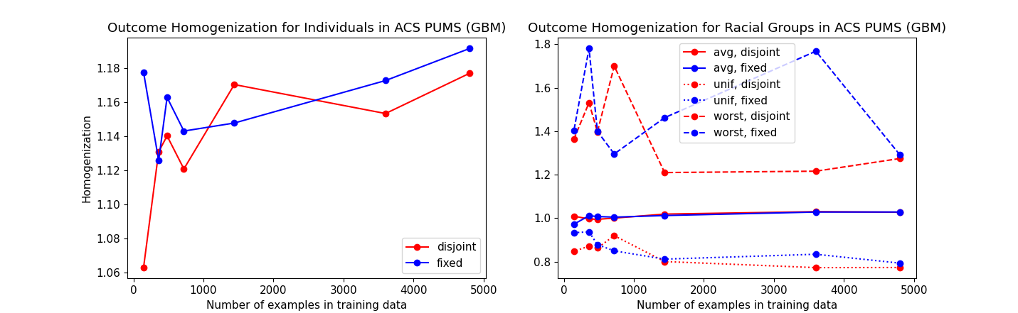
Figure 4: Results for data-sharing experiments on ACS PUMS with gradient boosted classifiers showing homogenization ($y$) as a function of training dataset size ($x$). Training across tasks on the same data (fixed) yields more homogeneous outcomes than on non-identical but identically distributed data (disjoint), especially for small datasets.

Figure 5: Results for data-sharing experiments on ACS PUMS with support vector machines showing homogenization ($y$) as a function of training dataset size ($x$). Training across tasks on the same data (fixed) yields more homogeneous outcomes than on non-identical but identically distributed data (disjoint), especially for small datasets.

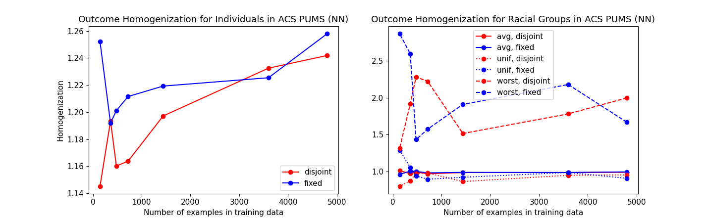
Figure 6: Results for data-sharing experiments on ACS PUMS with neural network classifiers showing homogenization ($y$) as a function of training dataset size ($x$). Training across tasks on the same data (fixed) yields more homogeneous outcomes than on non-identical but identically distributed data (disjoint), especially for small datasets.

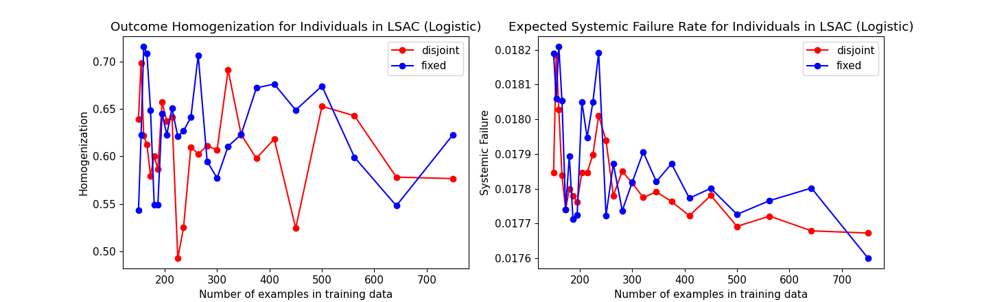
Figure 7: Results for data-sharing experiments on LSAC with logistic regression classifiers showing homogenization (left) and expected systemic failure rate $(\prod\limits_{i\in[k]}~{}\textsc{fail}(h^{i});\textbf{ right})$, which is the denominator in homogenization, as a function of training dataset size ($x$).

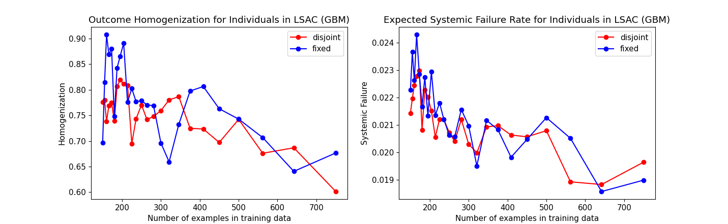
Figure 8: Results for data-sharing experiments on LSAC with gradient boosted classifiers showing homogenization (left) and expected systemic failure rate $(\prod\limits_{i\in[k]}~{}\textsc{fail}(h^{i});\textbf{ right})$, which is the denominator in homogenization, as a function of training dataset size ($x$).

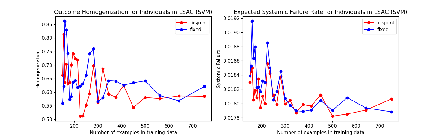
Figure 9: Results for data-sharing experiments on LSAC with support vector machines showing homogenization (left) and expected systemic failure rate $(\prod\limits_{i\in[k]}~{}\textsc{fail}(h^{i});\textbf{ right})$, which is the denominator in homogenization, as a function of training dataset size ($x$).

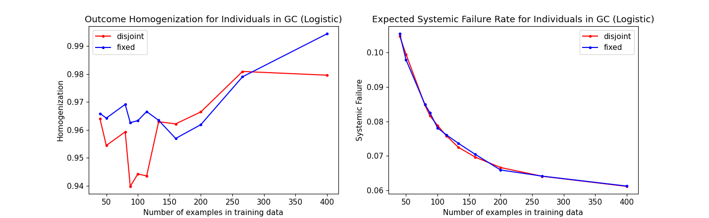
Figure 10: Results for data-sharing experiments on GC with logistic regression showing homogenization (left) and expected systemic failure rate $(\prod\limits_{i\in[k]}~{}\textsc{fail}(h^{i});\textbf{ right})$, which is the denominator in homogenization, as a function of training dataset size ($x$).

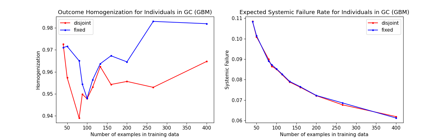
Figure 11: Results for data-sharing experiments on GC with gradient boosted classifiers showing homogenization (left) and expected systemic failure rate $(\prod\limits_{i\in[k]}~{}\textsc{fail}(h^{i});\textbf{ right})$, which is the denominator in homogenization, as a function of training dataset size ($x$).

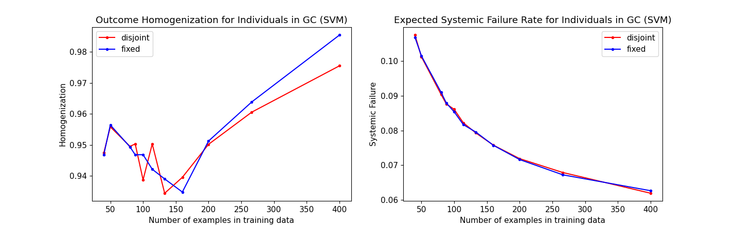
Figure 12: Results for data-sharing experiments on GC with support vector machines showing homogenization (left) and expected systemic failure rate $(\prod\limits_{i\in[k]}~{}\textsc{fail}(h^{i});\textbf{ right})$, which is the denominator in homogenization, as a function of training dataset size ($x$).

Results and Analysis.

We report additional results for ACS PUMS in Figures  4–6, for LSAC in Figures 7–9, and for GC in Figures 10–1. Across these figures, we first establish that our core findings are upheld: (i) homogenization is reliably greater when there is more homogenized (fixed) than less (disjoint) across datasets and model families and (ii) homogenization is reliably greater when contrasting individual-level measures with the appropriate racial group-level measures. However, we do note the absolute scale of homogenization is quite different across the datasets: we note that this is not surprising given the datasets are quite different, as are the relationship between the prediction tasks within a dataset. Therefore, we highlight that our hypotheses make predictions about relative change (i.e. sharing increases homogenization), but the underlying homogenization and absolute quantities will also depend significantly on the structure of the data and relationship between prediction tasks.

Further, for the LSAC and GC datasets, we visualize how the expected systemic failure rate (i.e. the product of the error rates of the models, which is the denominator in our homogenization metric) changes as a function of data scale. What we find is for both datasets, even one we have sufficient samples that the systemic failure rates in both the disjoint and fixed settings are identical (i.e. variance due to finite sample effects in error rates becomes minimal), we see higher homogenization. This demonstrates an important point: as the data grows, the expected systemic failure rate converges (as expected) to the same value for the disjoint and fixed partitions. That is, if one pays attention only to the accuracies for each task, these systems are the same. But even at this state, we see sizable discrepancies in outcome homogenization (i.e. the observed systemic failure rates remain different) with the fixed partition displaying greater homogenization. This drives home the point that data-sharing here has no effect on the accuracies of the resultant models, but that it does yield greater homogenization. This demonstration is reminscent of work that demonstrates the existence of models of (near) equal accuracy but that are simpler [Semenova et al., 2022] or more fair [Marx et al., 2020]. Here we observe a Rashomon effect [Breiman, 2001] at the level of social systems: both systems achieve the same accuracies, but one (disjoint) is more homogeneous than the other (fixed).

References

- Kleinberg and Raghavan [2021] Jon Kleinberg and Manish Raghavan. Algorithmic monoculture and social welfare. Proceedings of the National Academy of Sciences, 118(22), 2021. ISSN 0027-8424. doi: 10.1073/pnas.2018340118. URL https://www.pnas.org/content/118/22/e2018340118.
- Moore and Tambini [2018] Martin Moore and Damian Tambini, editors. Digital Dominance: The Power of Google, Facebook, Amazon and Apple. Oxford University Press, New York, NY, 05 2018. ISBN 9780190845131.
- Engler [2021] Alex Engler. Enrollment algorithms are contributing to the crises of higher education. report, The Brookings Institution, September 2021. URL https://www.brookings.edu/research/enrollment-algorithms-are-contributing-to-the-crises-of-higher-education/.
- Bommasani et al. [2021] Rishi Bommasani, Drew A. Hudson, Ehsan Adeli, Russ Altman, Simran Arora, Sydney von Arx, Michael S. Bernstein, Jeannette Bohg, Antoine Bosselut, Emma Brunskill, Erik Brynjolfsson, S. Buch, D. Card, Rodrigo Castellon, Niladri S. Chatterji, Annie Chen, Kathleen Creel, Jared Davis, Dora Demszky, Chris Donahue, Moussa Doumbouya, Esin Durmus, Stefano Ermon, John Etchemendy, Kawin Ethayarajh, Li Fei-Fei, Chelsea Finn, Trevor Gale, Lauren E. Gillespie, Karan Goel, Noah D. Goodman, Shelby Grossman, Neel Guha, Tatsunori Hashimoto, Peter Henderson, John Hewitt, Daniel E. Ho, Jenny Hong, Kyle Hsu, Jing Huang, Thomas F. Icard, Saahil Jain, Dan Jurafsky, Pratyusha Kalluri, Siddharth Karamcheti, Geoff Keeling, Fereshte Khani, O. Khattab, Pang Wei Koh, Mark S. Krass, Ranjay Krishna, Rohith Kuditipudi, Ananya Kumar, Faisal Ladhak, Mina Lee, Tony Lee, Jure Leskovec, Isabelle Levent, Xiang Lisa Li, Xuechen Li, Tengyu Ma, Ali Malik, Christopher D. Manning, Suvir P. Mirchandani, Eric Mitchell, Zanele Munyikwa, Suraj Nair, Avanika Narayan, Deepak Narayanan, Ben Newman, Allen Nie, Juan Carlos Niebles, Hamed Nilforoshan, J. F. Nyarko, Giray Ogut, Laurel Orr, Isabel Papadimitriou, Joon Sung Park, Chris Piech, Eva Portelance, Christopher Potts, Aditi Raghunathan, Robert Reich, Hongyu Ren, Frieda Rong, Yusuf H. Roohani, Camilo Ruiz, Jackson K. Ryan, Christopher R’e, Dorsa Sadigh, Shiori Sagawa, Keshav Santhanam, Andy Shih, Krishna Parasuram Srinivasan, Alex Tamkin, Rohan Taori, Armin W. Thomas, Florian Tramèr, Rose E. Wang, William Wang, Bohan Wu, Jiajun Wu, Yuhuai Wu, Sang Michael Xie, Michihiro Yasunaga, Jiaxuan You, Matei A. Zaharia, Michael Zhang, Tianyi Zhang, Xikun Zhang, Yuhui Zhang, Lucia Zheng, Kaitlyn Zhou, and Percy Liang. On the opportunities and risks of foundation models. ArXiv, abs/2108.07258, 2021. URL https://crfm.stanford.edu/assets/report.pdf.
- Kasy and Abebe [2021] Maximilian Kasy and Rediet Abebe. Fairness, equality, and power in algorithmic decision-making. In Proceedings of the 2021 ACM Conference on Fairness, Accountability, and Transparency, FAccT ’21, page 576–586, New York, NY, USA, 2021. Association for Computing Machinery. ISBN 9781450383097. doi: 10.1145/3442188.3445919. URL https://doi.org/10.1145/3442188.3445919.
- Jowell and Prescott-Clarke [1970] Roger Jowell and Patricia Prescott-Clarke. Racial discrimination and white-collar workers in britain. Race, 11(4):397–417, April 1970. doi: 10.1177/030639687001100401. URL https://doi.org/10.1177/030639687001100401.
- Bertrand and Mullainathan [2004] Marianne Bertrand and Sendhil Mullainathan. Are emily and greg more employable than lakisha and jamal? a field experiment on labor market discrimination. American Economic Review, 94(4):991–1013, August 2004. doi: 10.1257/0002828042002561. URL https://doi.org/10.1257/0002828042002561.
- Kline et al. [2021] Patrick Kline, Evan Rose, and Christopher Walters. Systemic discrimination among large u.s. employers. Technical report, National Bureau of Economic Research, July 2021. URL https://doi.org/10.3386/w29053.
- Sonderling et al. [2022] Keith E. Sonderling, Bradford J. Kelley, and Lance Casimir. The promise and the peril: Artificial intelligence and employment discrimination. University of Miami Law Review, 77, 11 2022. URL https://repository.law.miami.edu/umlr/vol77/iss1/3.
- Hirevue [2021] Hirevue. Hirevue customers conduct over 1 million video interviews in just 30 days, Oct 2021. URL https://www.hirevue.com/press-release/hirevue-customers-conduct-over-1-million-video-interviews-in-just-30-days.
- Creel and Hellman [2022] Kathleen Creel and Deborah Hellman. The algorithmic leviathan: Arbitrariness, fairness, and opportunity in algorithmic decision-making systems. Canadian Journal of Philosophy, 52(1):26–43, 2022. doi: 10.1017/can.2022.3.
- Campbell and Fiske [1959] Donald T. Campbell and Donald W. Fiske. Convergent and discriminant validation by the multitrait-multimethod matrix. Psychological Bulletin, 56(2):81, 1959. URL https://pubmed.ncbi.nlm.nih.gov/13634291/.
- Messick [1987] Samuel Messick. Validity. ETS Research Report Series, 1987(2):i–208, 1987. URL https://onlinelibrary.wiley.com/doi/abs/10.1002/j.2330-8516.1987.tb00244.x.
- Jacobs and Wallach [2021] Abigail Z. Jacobs and Hanna Wallach. Measurement and fairness. In Proceedings of the 2021 Conference on Fairness, Accountability, and Transparency, FAccT ’21, New York, NY, USA, 2021. Association for Computing Machinery. URL https://arxiv.org/abs/1912.05511.
- Zhao and Chen [2019] Chen Zhao and Feng Chen. Rank-based multi-task learning for fair regression. In 2019 IEEE International Conference on Data Mining (ICDM), pages 916–925, 2019. doi: 10.1109/ICDM.2019.00102.
- D’Amour et al. [2020] Alexander D’Amour, Katherine A. Heller, Dan I. Moldovan, Ben Adlam, Babak Alipanahi, Alex Beutel, Christina Chen, Jonathan Deaton, Jacob Eisenstein, Matthew D. Hoffman, Farhad Hormozdiari, Neil Houlsby, Shaobo Hou, Ghassen Jerfel, Alan Karthikesalingam, Mario Lucic, Yi-An Ma, Cory Y. McLean, Diana Mincu, Akinori Mitani, Andrea Montanari, Zachary Nado, Vivek Natarajan, Christopher Nielson, Thomas F. Osborne, Rajiv Raman, Kim Ramasamy, Rory Sayres, Jessica Schrouff, Martin G. Seneviratne, Shannon Sequeira, Harini Suresh, Victor Veitch, Max Vladymyrov, Xuezhi Wang, Kellie Webster, Steve Yadlowsky, Taedong Yun, Xiaohua Zhai, and D. Sculley. Underspecification presents challenges for credibility in modern machine learning. ArXiv, abs/2011.03395, 2020.
- Wang et al. [2021] Yuyan Wang, Xuezhi Wang, Alex Beutel, Flavien Prost, Jilin Chen, and Ed H. Chi. Understanding and Improving Fairness-Accuracy Trade-Offs in Multi-Task Learning, page 1748–1757. Association for Computing Machinery, New York, NY, USA, 2021. ISBN 9781450383325. URL https://doi.org/10.1145/3447548.3467326.
- Dwork et al. [2012] Cynthia Dwork, Moritz Hardt, Toniann Pitassi, Omer Reingold, and Richard Zemel. Fairness through awareness. In Proceedings of the 3rd Innovations in Theoretical Computer Science Conference, ITCS ’12, page 214–226, New York, NY, USA, 2012. Association for Computing Machinery. ISBN 9781450311151. doi: 10.1145/2090236.2090255. URL https://doi.org/10.1145/2090236.2090255.
- Hardt et al. [2016] Moritz Hardt, Eric Price, and Nathan Srebro. Equality of opportunity in supervised learning. In NIPS, 2016.
- Sagawa* et al. [2020] Shiori Sagawa*, Pang Wei Koh*, Tatsunori B. Hashimoto, and Percy Liang. Distributionally robust neural networks. In International Conference on Learning Representations, 2020. URL https://openreview.net/forum?id=ryxGuJrFvS.
- Fabris et al. [2022] Alessandro Fabris, Stefano Messina, Gianmaria Silvello, and Gian Antonio Susto. Algorithmic fairness datasets: the story so far. Data Mining and Knowledge Discovery, abs/2202.01711, 2022.
- Dua and Graff [2017] Dheeru Dua and Casey Graff. UCI machine learning repository, 2017. URL http://archive.ics.uci.edu/ml.
- Ding et al. [2021] Frances Ding, Moritz Hardt, John Miller, and Ludwig Schmidt. Retiring adult: New datasets for fair machine learning. In Thirty-Fifth Conference on Neural Information Processing Systems, 2021. URL https://openreview.net/forum?id=bYi_2708mKK.
- Wightman et al. [1998] L.F. Wightman, H. Ramsey, and Law School Admission Council. LSAC National Longitudinal Bar Passage Study. LSAC research report series. Law School Admission Council, 1998. URL https://books.google.com/books?id=dtA7AQAAIAAJ.
- Kearns et al. [2018] Michael Kearns, Seth Neel, Aaron Roth, and Zhiwei Steven Wu. Preventing fairness gerrymandering: Auditing and learning for subgroup fairness. In Jennifer Dy and Andreas Krause, editors, Proceedings of the 35th International Conference on Machine Learning, volume 80 of Proceedings of Machine Learning Research, pages 2564–2572. PMLR, 10–15 Jul 2018. URL https://proceedings.mlr.press/v80/kearns18a.html.
- Hashimoto et al. [2018] Tatsunori B. Hashimoto, Megha Srivastava, Hongseok Namkoong, and Percy Liang. Fairness without demographics in repeated loss minimization. In ICML, 2018.
- Crenshaw [1989] Kimberlé Crenshaw. Demarginalizing the intersection of race and sex: A black feminist critique of antidiscrimination doctrine, feminist theory and antiracist politics. University of Chicago Legal Forum, Vol.1989, Article 8, 1989. URL https://chicagounbound.uchicago.edu/cgi/viewcontent.cgi?article=1052&context=uclf.
- Fishman and Hancox-Li [2022] Nic Fishman and Leif Hancox-Li. Should attention be all we need? the epistemic and ethical implications of unification in machine learning. In Proceedings of the 2022 Conference on Fairness, Accountability, and Transparency, FAccT ’22, New York, NY, USA, 2022. Association for Computing Machinery. URL https://arxiv.org/abs/2205.08377.
- Liu et al. [2015] Ziwei Liu, Ping Luo, Xiaogang Wang, and Xiaoou Tang. Deep learning face attributes in the wild. 2015 IEEE International Conference on Computer Vision (ICCV), pages 3730–3738, 2015.
- Khani and Liang [2021] Fereshte Khani and Percy Liang. Removing spurious features can hurt accuracy and affect groups disproportionately. In Proceedings of the 2021 ACM Conference on Fairness, Accountability, and Transparency, FAccT ’21, page 196–205, New York, NY, USA, 2021. Association for Computing Machinery. ISBN 9781450383097. doi: 10.1145/3442188.3445883. URL https://doi.org/10.1145/3442188.3445883.
- Gururangan et al. [2019] Suchin Gururangan, Tam Dang, Dallas Card, and Noah A. Smith. Variational pretraining for semi-supervised text classification. In Proceedings of the 57th Annual Meeting of the Association for Computational Linguistics, pages 5880–5894, Florence, Italy, July 2019. Association for Computational Linguistics. doi: 10.18653/v1/P19-1590. URL https://aclanthology.org/P19-1590.
- Maas et al. [2011] Andrew L. Maas, Raymond E. Daly, Peter T. Pham, Dan Huang, Andrew Y. Ng, and Christopher Potts. Learning word vectors for sentiment analysis. In Proceedings of the 49th Annual Meeting of the Association for Computational Linguistics: Human Language Technologies, pages 142–150, Portland, Oregon, USA, June 2011. Association for Computational Linguistics. URL http://www.aclweb.org/anthology/P11-1015.
- Zhang et al. [2015] Xiang Zhang, Junbo Zhao, and Yann LeCun. Character-level convolutional networks for text classification. In C. Cortes, N. Lawrence, D. Lee, M. Sugiyama, and R. Garnett, editors, Advances in Neural Information Processing Systems, volume 28. Curran Associates, Inc., 2015. URL https://proceedings.neurips.cc/paper/2015/file/250cf8b51c773f3f8dc8b4be867a9a02-Paper.pdf.
- Chang et al. [2008] Ming-Wei Chang, Lev Ratinov, Dan Roth, and Vivek Srikumar. Importance of semantic representation: Dataless classification. In Proceedings of the 23rd National Conference on Artificial Intelligence - Volume 2, AAAI’08, page 830–835. AAAI Press, 2008. ISBN 9781577353683.
- de Gibert et al. [2018] Ona de Gibert, Naiara Perez, Aitor García-Pablos, and Montse Cuadros. Hate Speech Dataset from a White Supremacy Forum. In Proceedings of the 2nd Workshop on Abusive Language Online (ALW2), pages 11–20, Brussels, Belgium, October 2018. Association for Computational Linguistics. doi: 10.18653/v1/W18-5102. URL https://www.aclweb.org/anthology/W18-5102.
- Radford et al. [2021] Alec Radford, Jong Wook Kim, Chris Hallacy, Aditya Ramesh, Gabriel Goh, Sandhini Agarwal, Girish Sastry, Amanda Askell, Pamela Mishkin, Jack Clark, Gretchen Krueger, and Ilya Sutskever. Learning transferable visual models from natural language supervision. In ICML, 2021.
- Dosovitskiy et al. [2021] Alexey Dosovitskiy, Lucas Beyer, Alexander Kolesnikov, Dirk Weissenborn, Xiaohua Zhai, Thomas Unterthiner, Mostafa Dehghani, Matthias Minderer, Georg Heigold, Sylvain Gelly, Jakob Uszkoreit, and Neil Houlsby. An image is worth 16x16 words: Transformers for image recognition at scale. In International Conference on Learning Representations, 2021. URL https://openreview.net/forum?id=YicbFdNTTy.
- Liu et al. [2019] Yinhan Liu, Myle Ott, Naman Goyal, Jingfei Du, Mandar Joshi, Danqi Chen, Omer Levy, Mike Lewis, Luke Zettlemoyer, and Veselin Stoyanov. Roberta: A robustly optimized bert pretraining approach. ArXiv, abs/1907.11692, 2019.
- Ben Zaken et al. [2022] Elad Ben Zaken, Yoav Goldberg, and Shauli Ravfogel. BitFit: Simple parameter-efficient fine-tuning for transformer-based masked language-models. In Proceedings of the 60th Annual Meeting of the Association for Computational Linguistics (Volume 2: Short Papers), pages 1–9, Dublin, Ireland, May 2022. Association for Computational Linguistics. URL https://aclanthology.org/2022.acl-short.1.
- Kumar et al. [2022] Ananya Kumar, Aditi Raghunathan, Robbie Matthew Jones, Tengyu Ma, and Percy Liang. Fine-tuning can distort pretrained features and underperform out-of-distribution. In International Conference on Learning Representations, 2022. URL https://openreview.net/forum?id=UYneFzXSJWh.
- Khani et al. [2019] Fereshte Khani, Aditi Raghunathan, and Percy Liang. Maximum weighted loss discrepancy. ArXiv, abs/1906.03518, 2019.
- Anderson [1999] Elizabeth S. Anderson. What is the point of equality? Ethics, 109(2):287–337, January 1999. doi: 10.1086/233897. URL https://doi.org/10.1086/233897.
- Anderson [2016] Elizabeth Anderson. Liberty, Equality, and Private Government. University of Utah Press, 2016.
- Birhane [2021] Abeba Birhane. Algorithmic injustice: a relational ethics approach. Patterns, 2(2):100205, 2021. ISSN 2666-3899. doi: https://doi.org/10.1016/j.patter.2021.100205. URL https://www.sciencedirect.com/science/article/pii/S2666389921000155.
- Viljoen [2021] Salomé Viljoen. A relational theory of data governance. Yale Law Journal, 131(2), 2021.
- Fish and Stark [2022] Benjamin Fish and Luke Stark. It’s not fairness, and it’s not fair: The failure of distributional equality and the promise of relational equality in complete-information hiring games. In Equity and Access in Algorithms, Mechanisms, and Optimization, EAAMO ’22, New York, NY, USA, 2022. Association for Computing Machinery. ISBN 9781450394772. doi: 10.1145/3551624.3555296. URL https://doi.org/10.1145/3551624.3555296.
- Raz [1988] Joseph Raz. The Morality of Freedom. Oxford University Press, Oxford, 1988.
- Buolamwini and Gebru [2018] Joy Buolamwini and Timnit Gebru. Gender shades: Intersectional accuracy disparities in commercial gender classification. In Sorelle A. Friedler and Christo Wilson, editors, Proceedings of the 1st Conference on Fairness, Accountability and Transparency, volume 81 of Proceedings of Machine Learning Research, pages 77–91. PMLR, 23–24 Feb 2018. URL https://proceedings.mlr.press/v81/buolamwini18a.html.
- Raji and Buolamwini [2019] Inioluwa Deborah Raji and Joy Buolamwini. Actionable auditing: Investigating the impact of publicly naming biased performance results of commercial ai products. In Proceedings of the 2019 AAAI/ACM Conference on AI, Ethics, and Society, AIES ’19, page 429–435, New York, NY, USA, 2019. Association for Computing Machinery. ISBN 9781450363242. doi: 10.1145/3306618.3314244. URL https://doi.org/10.1145/3306618.3314244.
- Metaxa et al. [2021] Danaë Metaxa, Joon Sung Park, Ronald E. Robertson, Karrie Karahalios, Christo Wilson, Jeff Hancock, and Christian Sandvig. Auditing algorithms: Understanding algorithmic systems from the outside in. Foundations and Trends® in Human–Computer Interaction, 14(4):272–344, 2021. ISSN 1551-3955. doi: 10.1561/1100000083. URL http://dx.doi.org/10.1561/1100000083.
- Loevinger [1957] Jane Loevinger. Objective tests as instruments of psychological theory. Psychological Reports, 3(3):635–694, 1957. doi: 10.2466/pr0.1957.3.3.635. URL https://doi.org/10.2466/pr0.1957.3.3.635.
- Hand [2016] D.J. Hand. Measurement: A Very Short Introduction. Very short introductions. Oxford University Press, 2016. ISBN 9780198779568. URL https://books.google.com/books?id=QBIBDQAAQBAJ.
- Dubins and Spanier [1961] L. E. Dubins and E. H. Spanier. How to cut a cake fairly. The American Mathematical Monthly, 68(1):1–17, 1961. ISSN 00029890, 19300972. URL http://www.jstor.org/stable/2311357.
- Henzinger et al. [2022] Monika Henzinger, Charlotte Peale, Omer Reingold, and Judy Hanwen Shen. Leximax approximations and representative cohort selection. ArXiv, abs/2205.01157, 2022.
- Pedregosa et al. [2011] Fabian Pedregosa, Gaël Varoquaux, Alexandre Gramfort, Vincent Michel, Bertrand Thirion, Olivier Grisel, Mathieu Blondel, Peter Prettenhofer, Ron Weiss, Vincent Dubourg, Jake Vanderplas, Alexandre Passos, David Cournapeau, Matthieu Brucher, Matthieu Perrot, and Édouard Duchesnay. Scikit-learn: Machine learning in python. Journal of Machine Learning Research, 12(85):2825–2830, 2011. URL http://jmlr.org/papers/v12/pedregosa11a.html.
- Birhane and Prabhu [2021] Abeba Birhane and Vinay Uday Prabhu. Large image datasets: A pyrrhic win for computer vision? In 2021 IEEE Winter Conference on Applications of Computer Vision (WACV), pages 1536–1546, 2021. doi: 10.1109/WACV48630.2021.00158.
- Birhane et al. [2021] Abeba Birhane, Vinay Uday Prabhu, and Emmanuel Kahembwe. Multimodal datasets: misogyny, pornography, and malignant stereotypes. ArXiv, abs/2110.01963, 2021.
- Lhoest et al. [2021] Quentin Lhoest, Albert Villanova del Moral, Yacine Jernite, Abhishek Thakur, Patrick von Platen, Suraj Patil, Julien Chaumond, Mariama Drame, Julien Plu, Lewis Tunstall, Joe Davison, Mario Šaško, Gunjan Chhablani, Bhavitvya Malik, Simon Brandeis, Teven Le Scao, Victor Sanh, Canwen Xu, Nicolas Patry, Angelina McMillan-Major, Philipp Schmid, Sylvain Gugger, Clément Delangue, Théo Matussière, Lysandre Debut, Stas Bekman, Pierric Cistac, Thibault Goehringer, Victor Mustar, François Lagunas, Alexander Rush, and Thomas Wolf. Datasets: A community library for natural language processing. In Proceedings of the 2021 Conference on Empirical Methods in Natural Language Processing: System Demonstrations, pages 175–184, Online and Punta Cana, Dominican Republic, November 2021. Association for Computational Linguistics. doi: 10.18653/v1/2021.emnlp-demo.21. URL https://aclanthology.org/2021.emnlp-demo.21.
- Wolf et al. [2020] Thomas Wolf, Lysandre Debut, Victor Sanh, Julien Chaumond, Clement Delangue, Anthony Moi, Pierric Cistac, Tim Rault, Remi Louf, Morgan Funtowicz, Joe Davison, Sam Shleifer, Patrick von Platen, Clara Ma, Yacine Jernite, Julien Plu, Canwen Xu, Teven Le Scao, Sylvain Gugger, Mariama Drame, Quentin Lhoest, and Alexander Rush. Transformers: State-of-the-art natural language processing. In Proceedings of the 2020 Conference on Empirical Methods in Natural Language Processing: System Demonstrations, pages 38–45, Online, October 2020. Association for Computational Linguistics. doi: 10.18653/v1/2020.emnlp-demos.6. URL https://aclanthology.org/2020.emnlp-demos.6.
- Shwartz et al. [2020] Vered Shwartz, Rachel Rudinger, and Oyvind Tafjord. “you are grounded!”: Latent name artifacts in pre-trained language models. In Proceedings of the 2020 Conference on Empirical Methods in Natural Language Processing (EMNLP), pages 6850–6861, Online, November 2020. Association for Computational Linguistics. doi: 10.18653/v1/2020.emnlp-main.556. URL https://aclanthology.org/2020.emnlp-main.556.
- Romanov et al. [2019] Alexey Romanov, Maria De-Arteaga, Hanna Wallach, Jennifer Chayes, Christian Borgs, Alexandra Chouldechova, Sahin Geyik, Krishnaram Kenthapadi, Anna Rumshisky, and Adam Kalai. What’s in a name? Reducing bias in bios without access to protected attributes. In Proceedings of the 2019 Conference of the North American Chapter of the Association for Computational Linguistics: Human Language Technologies, Volume 1 (Long and Short Papers), pages 4187–4195, Minneapolis, Minnesota, June 2019. Association for Computational Linguistics. doi: 10.18653/v1/N19-1424. URL https://aclanthology.org/N19-1424.
- Tzioumis [2018] Konstantinos Tzioumis. Demographic aspects of first names. Scientific Data, 5, 2018.
- Garg et al. [2018] Nikhil Garg, Londa Schiebinger, Dan Jurafsky, and James Zou. Word embeddings quantify 100 years of gender and ethnic stereotypes. Proceedings of the National Academy of Sciences, 115(16):E3635–E3644, 2018. ISSN 0027-8424. doi: 10.1073/pnas.1720347115. URL https://www.pnas.org/content/115/16/E3635.
- Cao and Daumé III [2020] Yang Trista Cao and Hal Daumé III. Toward gender-inclusive coreference resolution. In Proceedings of the 58th Annual Meeting of the Association for Computational Linguistics, pages 4568–4595, Online, July 2020. Association for Computational Linguistics. doi: 10.18653/v1/2020.acl-main.418. URL https://aclanthology.org/2020.acl-main.418.
- Antoniak and Mimno [2021] Maria Antoniak and David Mimno. Bad seeds: Evaluating lexical methods for bias measurement. In Proceedings of the 59th Annual Meeting of the Association for Computational Linguistics and the 11th International Joint Conference on Natural Language Processing (Volume 1: Long Papers), pages 1889–1904, Online, August 2021. Association for Computational Linguistics. doi: 10.18653/v1/2021.acl-long.148. URL https://aclanthology.org/2021.acl-long.148.
- Zhang and Yang [2017] Yu Zhang and Qiang Yang. A survey on multi-task learning. ArXiv, abs/1707.08114, 2017.
- Le Quy et al. [2022] Tai Le Quy, Arjun Roy, Vasileios Iosifidis, Wenbin Zhang, and Eirini Ntoutsi. A survey on datasets for fairness-aware machine learning. Wiley Interdisciplinary Reviews: Data Mining and Knowledge Discovery, 12, 05 2022. doi: 10.1002/widm.1452.
- Semenova et al. [2022] Lesia Semenova, Cynthia Rudin, and Ronald Parr. On the existence of simpler machine learning models. In 2022 ACM Conference on Fairness, Accountability, and Transparency, FAccT ’22, page 1827–1858, New York, NY, USA, 2022. Association for Computing Machinery. ISBN 9781450393522. doi: 10.1145/3531146.3533232. URL https://doi.org/10.1145/3531146.3533232.
- Marx et al. [2020] Charles T. Marx, Flavio Du Pin Calmon, and Berk Ustun. Predictive multiplicity in classification. In Proceedings of the 37th International Conference on Machine Learning, ICML’20. JMLR.org, 2020.
- Breiman [2001] L. Breiman. Statistical modeling: The two cultures. Quality Engineering, 48:81–82, 2001.