Four-dimensional differential equations for the leading divergences of dimensionally-regulated loop integrals

Abstract

We invent an automated method for computing the divergent part of Feynman integrals in dimensional regularization. Our method exploits simplifications from four-dimensional integration-by-parts identities. Leveraging algorithms from the literature, we show how to find simple differential equations for the divergent part of Feynman integrals that are free of subdivergences. We illustrate the method by an application to heavy quark effective theory at three loops.

1 Introduction

Our ability to evaluate Feynman integrals is crucial for computing perturbative results in quantum field theory. This subject has a long and rich history of various methods being developed Smirnov:2012gma . In recent years, the method of differential equations Kotikov:1990kg ; Bern:1992em ; Remiddi:1997ny ; Gehrmann:1999as has become the main method for evaluating loop integrals that are needed for collider phenomenology. In particular, insights about writing the differential equations in a canonical form Henn:2013pwa , has allowed both for an unprecedented degree of automation of the calculations, and has significantly pushed the boundaries of what is achievable.

Calculations are typically done within dimensional regularization, with $D=4-2\epsilon$, and the results are expanded in a Laurent series in the dimensional regulator $\epsilon$. One advantage of the differential equations method is at the same time a drawback: in principle, the differential equations describe the functions under consideration at any order in $\epsilon$. In practice, however, one often wishes to know results up the the finite part only, so that a lot of unnecessary information is kept at intermediate steps. What is more, the higher-order terms in $\epsilon$ are typically scheme-dependent, which means that they are more complicated than the physically relevant terms. Therefore it is desirable to develop methods that directly compute the physically relevant information, and profit from the simplifications.

Such a method exists for the case of (infrared- and ultraviolet-)finite Feynman integrals Caron-Huot:2014lda . The authors showed that it is possible to directly compute integration-by-parts-relations (IBP) in four dimensions, taking however special care about possible contact terms that relate integrals of different loop orders. There are several advantages to this. Firstly, the restriction of finite integrals means that significantly fewer integrals and IBP relations between them need to be considered, and the resulting number of master integrals is also less than in the conventional $D$-dimensional case. The simplifications in terms of handling the IBP relations in Caron-Huot:2014lda are so substantial that even certain three-loop four-point integrals with massive internal lines could be computed that were beyond the reach of conventional techniques. Secondly, when truncating to four dimensions, the canonical differential equations matrix takes a simple, ‘block-diagonal’ structure, which reflects transcendental weight of the different Feynman integrals. A similar decoupling of the differential equations was also noticed in Tancredi:2015pta . This makes it possible to iteratively solve for the master integrals, with increasing transcendental weight.

In many practical situations however, one often has to deal with divergent Feynman integrals. In the context of dimensional regularization, one is really interested in the coefficient functions appearing in the Laurent series in the dimensional regulator $\epsilon$. In practice, only a finite number of terms is needed. Therefore it would be desirable to have a method that directly computes those finite coefficient functions. Ideally, in order to profit from the advances mentioned above, this new method should be compatible with the canonical differential equations approach. Our aim is to develop such a method.

As a first step in this direction, in this paper we focus on Feynman integrals that are free from subdivergences, i.e. that in dimensional regularization only diverge as $1/\epsilon$, and we develop a four-dimensional integration-by-parts and canonical differential equation method for the coefficient function. We leave the generalization to the general case for future work. One might initially think that most Feynman diagrams have subdivergences, which limits the scope of the present paper. However, the structure of both ultraviolet (UV) and infrared divergences (IR) is very well understood, e.g. in terms of the famous Hopf algebra of renormalization Connes:1998qv , and in terms of factorization properties (see Catani:1996vz ; Dixon:2008gr ; Almelid:2015jia and references therein). Therefore, at least in principle, one could use our method on Feynman integrals in those cases as well, for some suitably-defined subtracted integrals (see e.g. Anastasiou:2018rib for recent work on an infrared subtraction for Feynman integrals).

We find it useful to focus on a particular type of divergences to present the new method. In this paper we focus on integrals in heavy quark effective theory (HQET). These integrals arise for example when massive particles emit soft radiation and capture infrared divergences associated to this radiation. Equivalently, they can be used to compute ultraviolet divergences of certain Wilson lines with cusp (related to the angle-dependent cusp anomalous dimension).

Working with these integrals as a case in point, we explain the main ingredients of our method. We first define HQET integrals that are free of subdivergences, and specify their leading divergence. We call the latter $I(\phi)$. Our goal is to compute $I(\phi)$. The main advantage of focusing on this coefficient, as opposed to the full Laurent expansion is that we can disregard unnecessary information. We explain how one obtains four-dimensional integration-by-parts (IBP) identities valid for $I(\phi)$. The master integrals appearing in these relations are all free of subdivergences of themselves, and there are less of them compared to the generic case. In this work, we develop a new syzygy IBP method to forbid integrals with soft divergence. (The original syzygy IBP method was developed to reduce an IBP system’s size Gluza:2010ws ; Schabinger:2011dz .)

Moreover, we find, as in Caron-Huot:2014lda , that there are integral identities that related different loop orders. As a result, the lower-loop information can be recycled. Using these simplified IBP relations, we obtain differential equations for the master integrals. Finally, we leverage ideas Dlapa:2020cwj of how to transform these equations into a simple canonical form.

This paper is organized as follows: in the section 2, we briefly review the Feynman integrals from web diagrams in HQET. In the section 3, our method of generating IBPs for the divergent part of Feynman integrals, based on graded IBP operators and syzygy, is introduced. In the section 4, we invent a four-dimensional version of the initial algorithm Dlapa:2020cwj , to generate canonical differential equations without $\epsilon$. In section 5, we provide a three-loop application of our method. Then we provide the summary and the outlook of our new method in the section 5.

2 From dimensionally-regularized Feynman diagrams to finite functions

Let us define the class of Feynman integrals that we study in this paper. We focus on integrals relevant for describing soft divergences occurring in the scattering of massive particles. These divergences can be described by an eikonal approximation, which leads to Wilson line correlators in position space. Equivalently, in momentum space, one obtains heavy-quark-effective theory (HQET) integrals Grozin:2015kna .

2.1 Cusped Wilson lines in position space

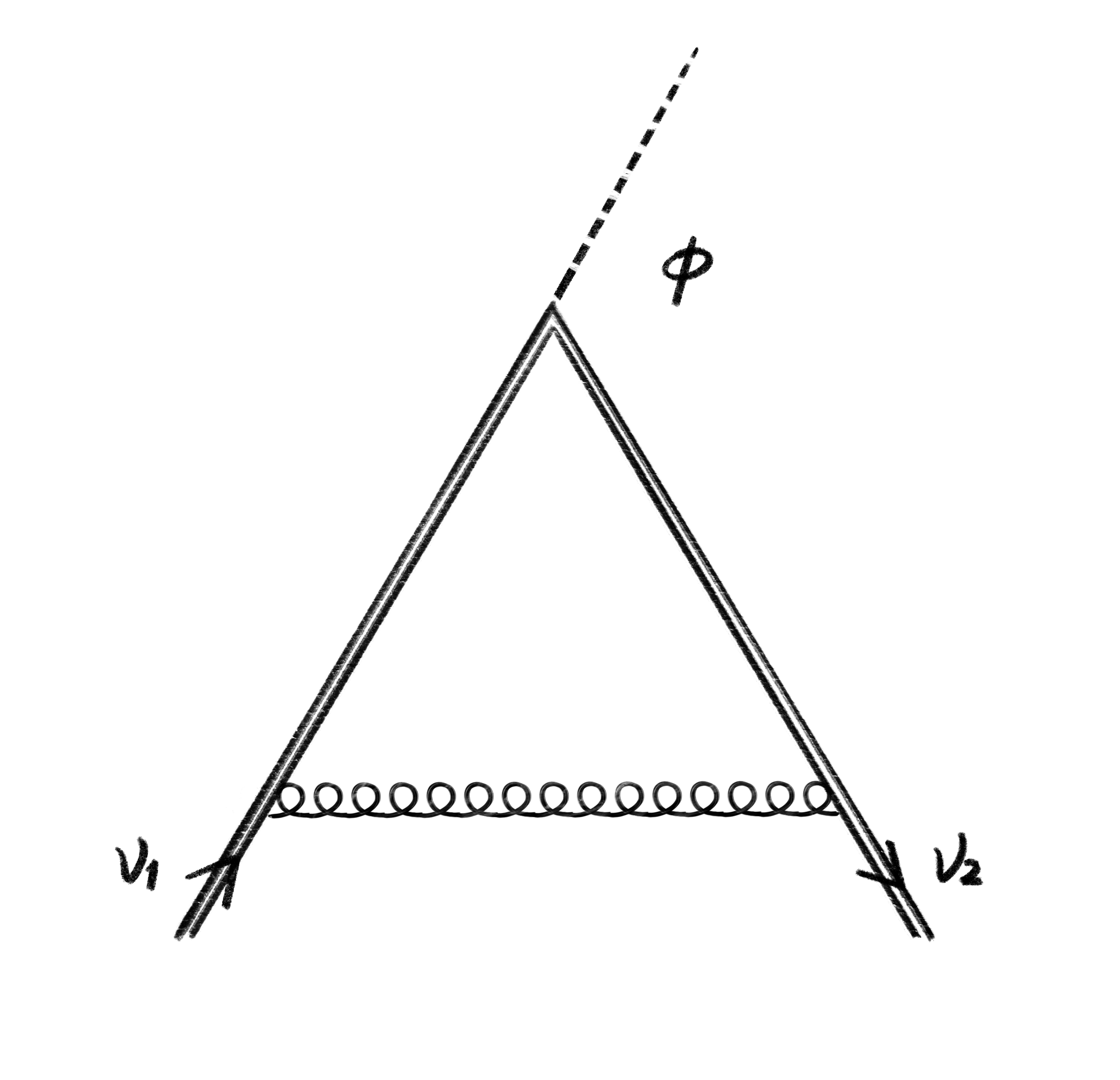
(a)

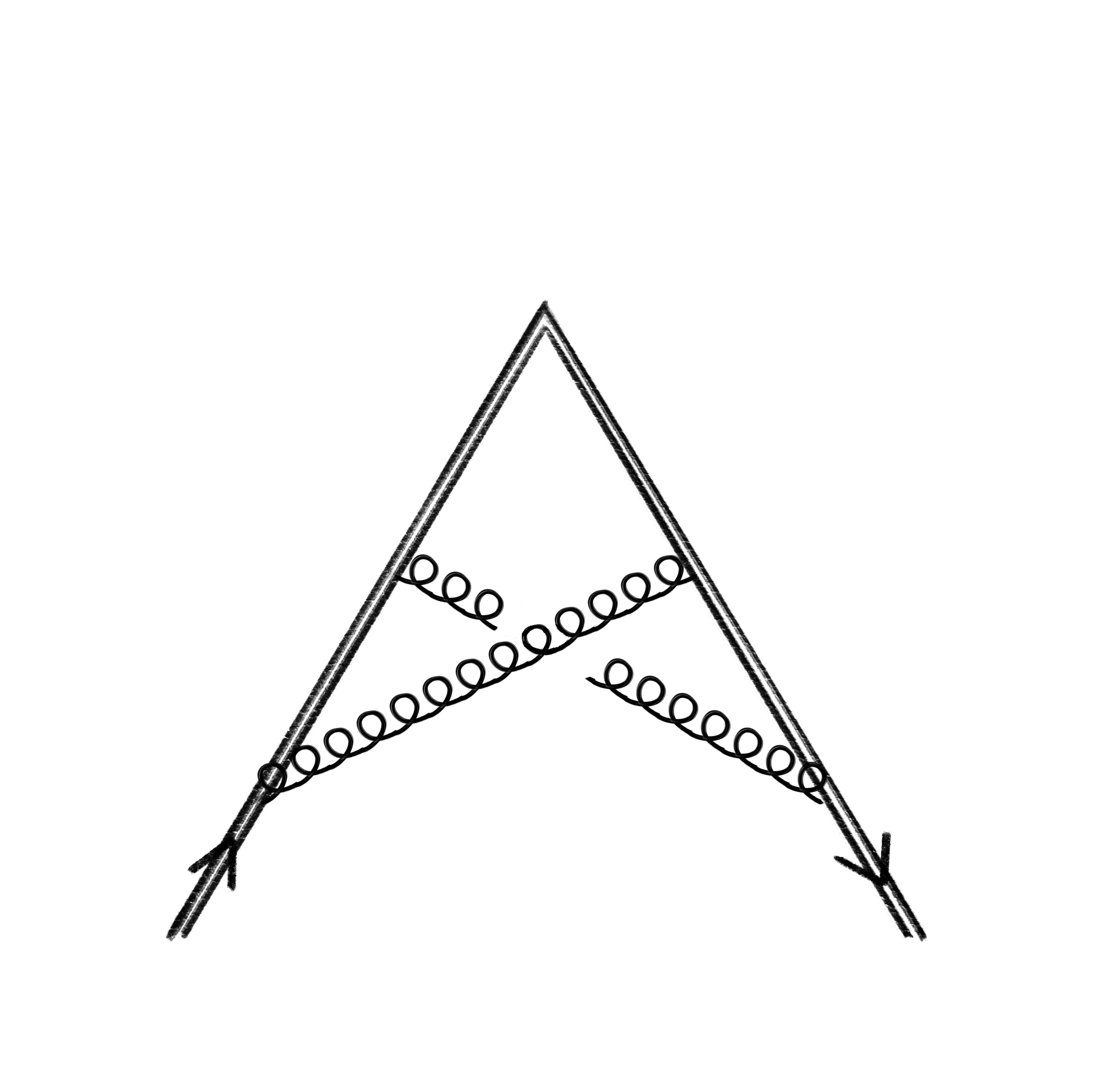
(b)

Figure 1: (a): One-loop Wilson line / heavy-quark effective theory diagram. (b) Example of a two-loop web diagram which has an overall divergence only.

Consider a soft exchange in the scattering of two massive particles. The leading divergence for such a process is given by the eikonal diagram in Fig. 1(a). It depends on the scattering angle $\phi$, and is given by

$$I^{(1)}(\phi,\epsilon)\sim\frac{1}{\epsilon}\phi\cot\phi+{\cal{O}}(\epsilon^{0})\,,\qquad{\rm where}\quad\cos\phi=\frac{v_{1}\cdot v_{2}}{\sqrt{v_{1}^{2}v_{2}^{2}}}\,.$$ (1)

In the following we set $v_{1}^{2}=v_{2}^{2}=1$ without loss of generality. The coefficient of the $1/\epsilon$ pole is the angle-dependent cusp anomalous dimension Polyakov:1980ca ; Brandt:1981kf ; Korchemsky:1987wg . Our goal is to compute the coefficient for this and similar higher-loop diagrams directly, using four-dimensional methods, without having to deal with the higher-order terms in $\epsilon$.

When extracting information from divergent Feynman integrals it is paramount to consider carefully whether the computational steps are consistent and well-defined. In principle, there are several sources of divergences in Feynman integrals, in particular ultraviolet (e.g. from renormalization of the Lagrangian or of composite operators) and infrared (soft and collinear divergences associated to massless particles). Here we will focus on Feynman integrals that have one type of divergence only, leaving the case of integrals with divergences in several simultaneous regions for future work.

The knowledge of what region of loop integration produces the divergences allows us to extract its coefficient in a well-defined way. Let us now illustrate this for the case of the one-loop integral shown in Fig. 1, and then explain how we approach the problem in general. In position space, the integral of Fig. 1(a) is given by

$$I^{(1)}(\phi,\epsilon)\sim\int_{0}^{\infty}d\tau_{1}d\tau_{2}\frac{v_{1}\cdot v_{2}}{[(\tau_{1}v_{1}+\tau_{2}v_{2})^{2}]^{1-\epsilon}}e^{-\tau_{1}-\tau_{2}}\,.$$ (2)

Here $e^{-\tau_{1}-\tau_{2}}$ is a cutoff that makes sure that the integral gives only the divergence at $\tau_{1},\tau_{2}\sim 0$ that is of interest to us. We can make the latter manifest by an overall rescaling,

$$I^{(1)}(\phi,\epsilon)\sim\underbrace{\int_{0}^{\infty}\frac{d\rho}{\rho^{1-\epsilon}}e^{-\rho}}_{1/\epsilon+{\cal O}(\epsilon^{0})}\times\underbrace{\int_{0}^{1}dz\frac{v_{1}\cdot v_{2}}{[(zv_{1}+(1-z)v_{2})^{2}]^{1-\epsilon}}}_{\phi\cot\phi+{\cal O}(\epsilon^{0})}\,.$$ (3)

2.2 HQET integrals in momentum space

One can equivalently write the integral discussed in subsection 2.1 in HQET language in momentum space. We briefly recall some notations of HQET (see Grozin:2004yc for a detailed review). HQET is an effective theory describing the dynamics of heavy quarks. In the heavy mass limit, the heavy quark’s propagator becomes

$$i\frac{\not{p}+m}{p^{2}-m^{2}+i\eta}\to i\frac{1+\not{v}}{2v\cdot k+i\eta}\,,$$ (4)

where $p=mv+k$. $v$ is the classical velocity of the heavy quark, normalized as $v^{2}=1$, while $k$ is its off-shell momentum. In this limit, the mass parameter factorizes out and the quantum field theory computation is simplified significantly. In practice, we may use an infrared regulator $\delta$ for the linear propagator in (4). Since $\delta$ is the only scale for the HQET integrals, it is safe to set $\delta=1$. In HQET language, diagram Fig. 1(a) is given by (up to an overall factor, $D=4-2\epsilon$)

$$I^{(1)}(\phi,\epsilon)\sim\int\frac{d^{D}k}{i\pi^{D/2}}\frac{1}{k^{2}(2k\cdot v_{1}+1)(2k\cdot v_{2}+1)}\,.$$ (5)

In eq. (5), the divergences comes from an overall rescaling where $k^{\mu}\sim\infty$. Now, in the above example, one could directly compute the coefficient of the $1/\epsilon$ pole by setting $\epsilon=0$ in the second factor of eq. (3). Something similar can be done in momentum space. We prefer however to develop a formalism that can be applied directly for covariant, four-dimensional Feynman integrals. The reason for this is that in this way we obtain a more general setup that we expect may be used for larger classes of Feynman integrals. For this reason we define

$$J^{(1)}(\phi)=\lim_{\epsilon\to 0}\left[\epsilon\,I^{(1)}(\phi,\epsilon)\right]\,.$$ (6)

Our goal is then to derive four-dimensional IBP relations that are valid for $J$.

2.3 Higher-loop diagrams free of subdivergences

Let us discuss the generalization to higher loops. Again, we focus on Feynman integrals with the divergence coming from one region of loop integration. In the case of our HQET integrals, we assume that they are free of subdivergences, and that the overall divergence is associated to a region where all loop momenta become large. See Fig. 1(b) for a two-loop example. Fig. 1(b) is an example of a so-called web diagram Frenkel:1984pz ; Gatheral:1983cz . By definition, webs do not have one-particle irreducible subdiagrams, which ensures the absence of subdivergences. Web diagrams occur naturally in the study of Wilson lines in the context of non-Abelian eikonal exponentiation Frenkel:1984pz ; Gatheral:1983cz . In a nutshell, they provide a setup for computing the cusp anomalous dimension from Feynman diagrams without subdivergences. So they are ideal objects to study for our purposes. To extract the overall divergence, we define in analogy to eq. (6),

$$J^{(L)}(\phi)=\lim_{\epsilon\to 0}\left[\epsilon\,I^{(L)}(\phi,\epsilon)\right]\,.$$ (7)

In this paper we focus on HQET web diagrams built from two eikonal lines (corresponding to the heavy quarks), and an arbitrary number of massless exchanges. We impose the following conditions on them:

1. The integrand has the overall scaling dimension $-4L$, for the transformation $k_{i}\to\lambda k_{i}$, $i=1,\ldots,L$. This follows from eikonal Feynman rules.

2. No UV divergence in any subloop subdiagram.

3. No infrared (IR) divergences. This forbids higher powers of massless propagators.

We call such integrals “admissible”. It follows from these properties that in dimensional regularization, admissible integrals have an overall $\epsilon^{-1}$ divergence only. We are interested in the coefficient of the divergence in (7).

2.4 Finding admissible integrals

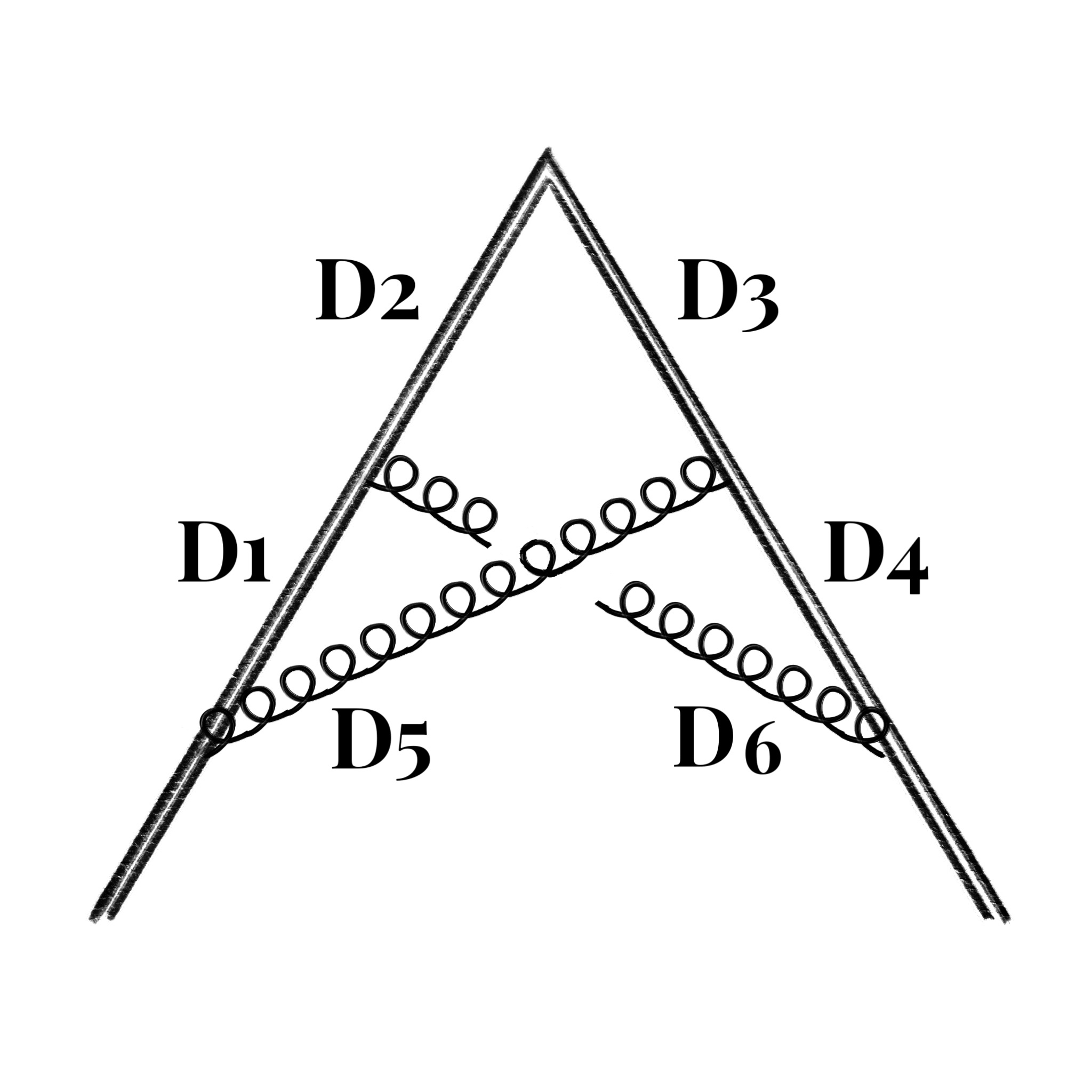
$A_{1}$

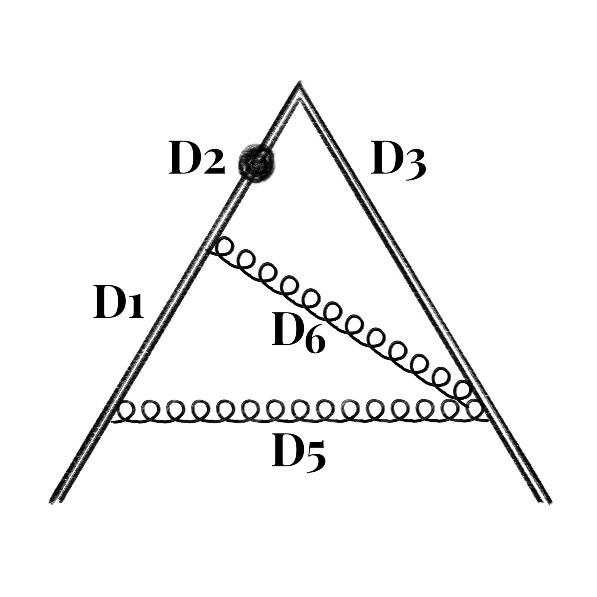
$B_{1}$

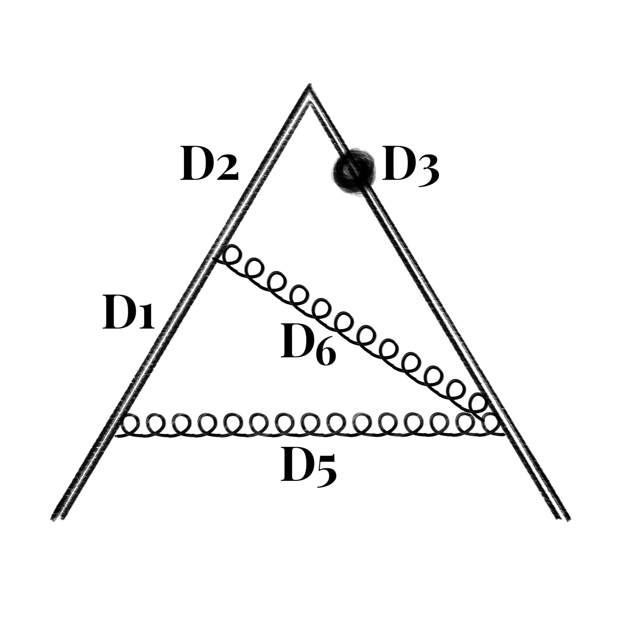
$B_{2}$

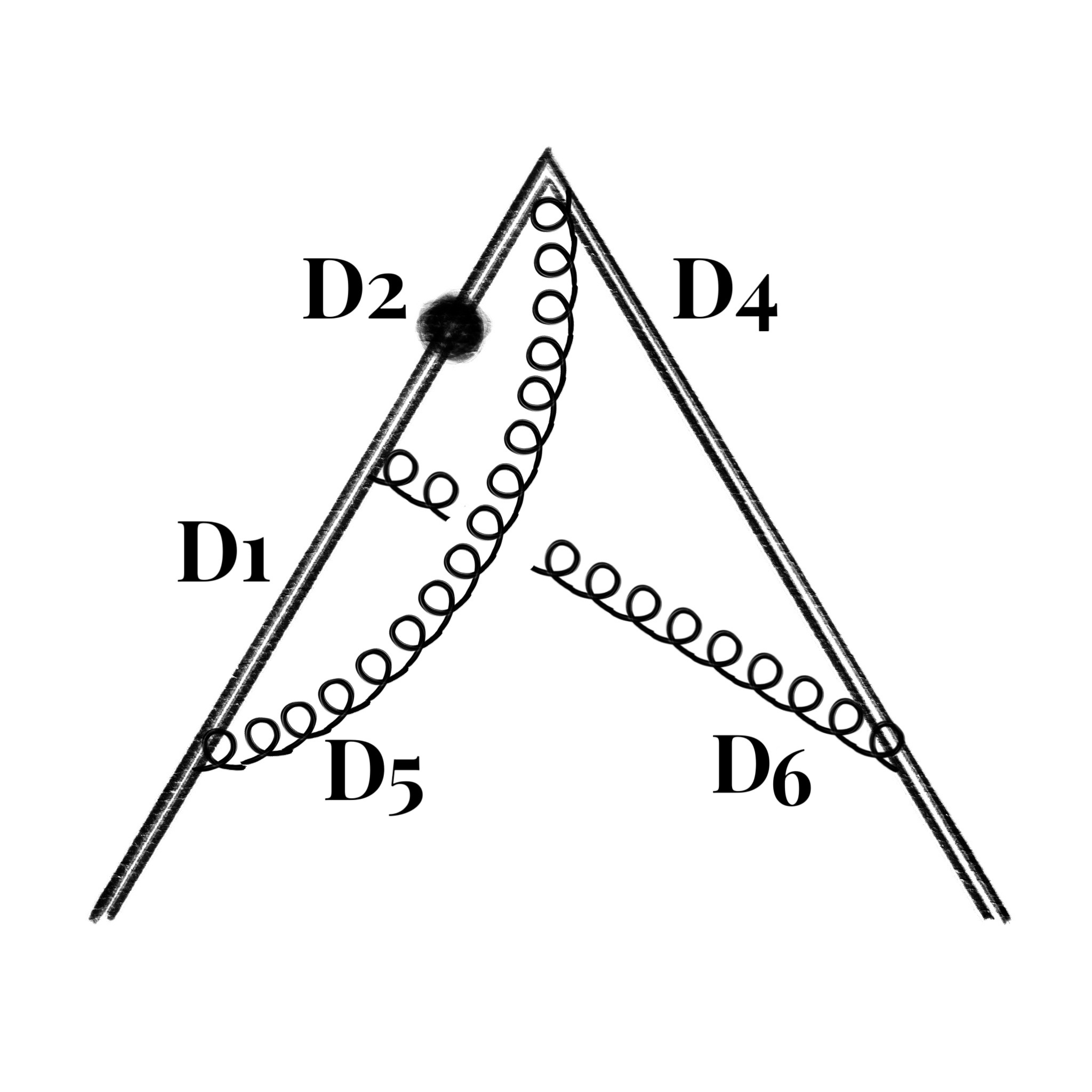
$B_{5}$

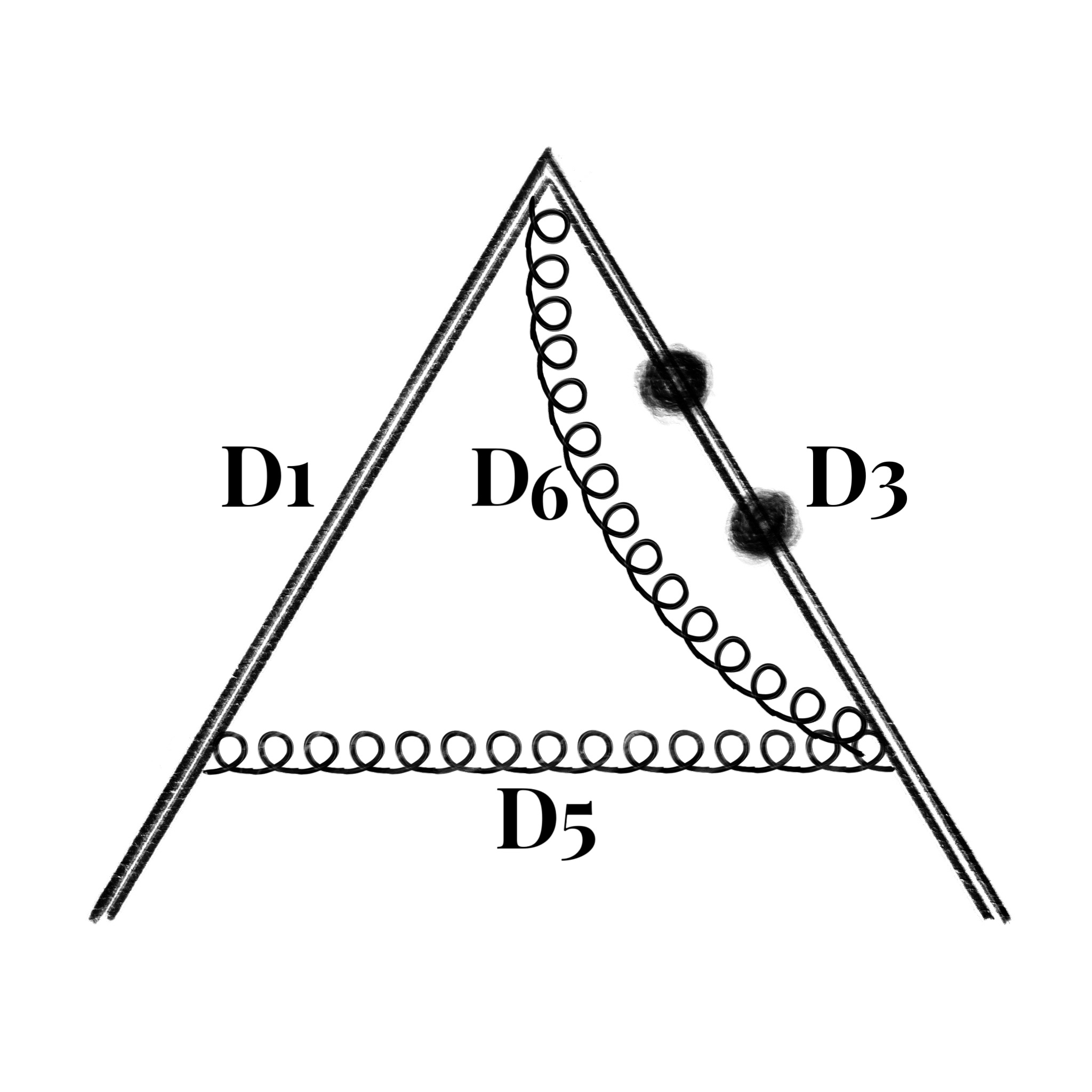
$C_{1}$

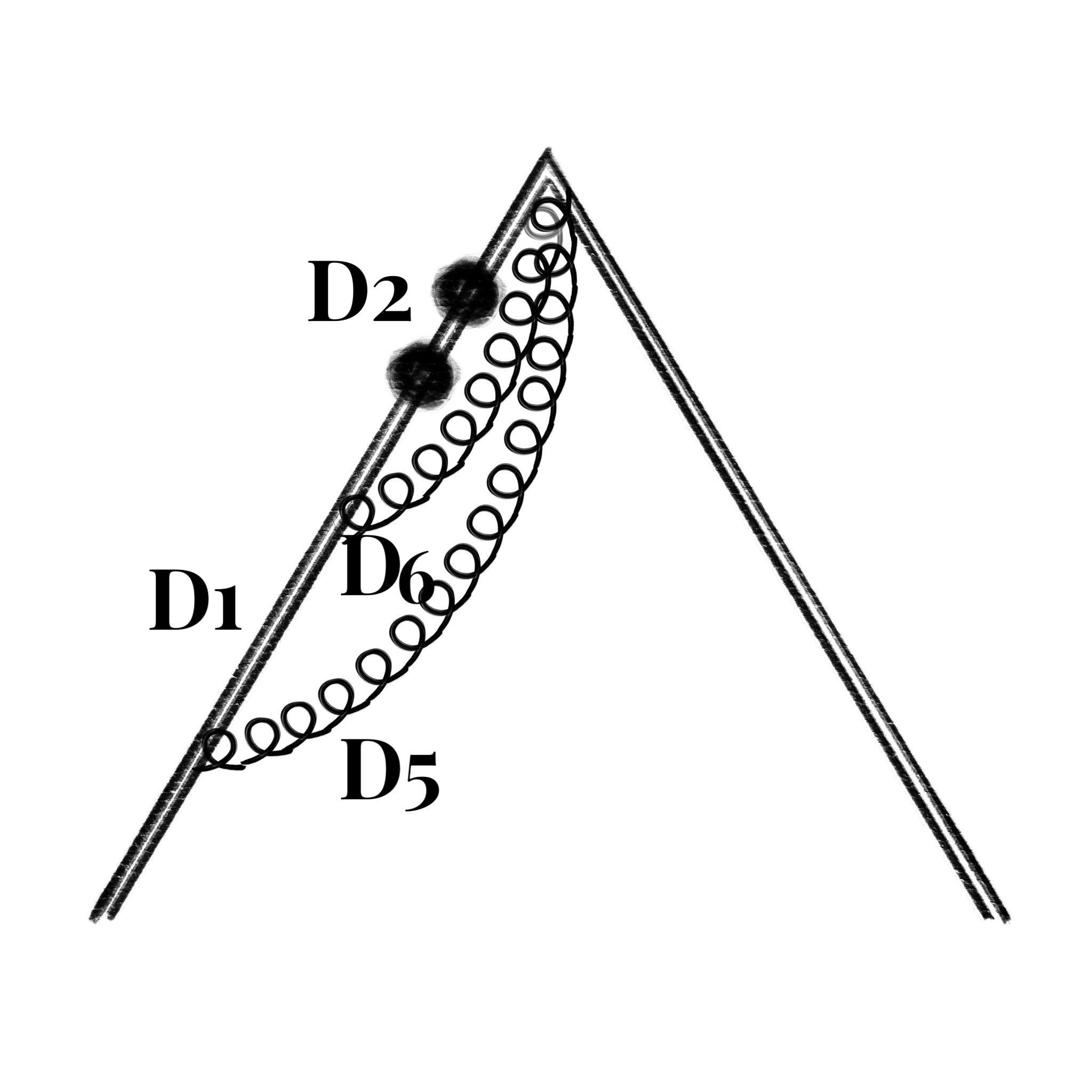
$C_{4}$

Figure 2: Admissible diagrams in the crossed ladder integral family. The dot stands for a doubled propagator. Further admissible integrals that involve numerator factors are given in the main text.

The three conditions formulated in subsection 2.3 can be translated to constraints on the Feynman integrals’ indices. While this restricts the space of integrals of interest to us, in general the solution space is infinite dimensional. In practice it is sufficient to work with a finite-dimensional subspace. We do this by placing further constraints on degrees of numerators or denominators. Then we can find all admissible integrals are subject to these additional conditions with the help of computer algebra.

Let us illustrate this for the diagram shown in Fig. 1(b). We define the crossed-ladder integral family ${\rm T^{(2)}}[a_{1},\cdots a_{7}]$ as follows.

$$\qquad{\rm T^{(2)}}[a_{1},\cdots,a_{7}]=\int\frac{d^{D}k_{1}}{i\pi^{D/2}}\frac{d^{D}k_{2}}{i\pi^{D/2}}\,\frac{D_{7}^{-a_{7}}}{D_{1}^{a_{1}}\,\cdots\,D_{6}^{a_{6}}}\,,\quad$$ (8)

where

$$D_{1} =-2k_{1}\cdot v_{1}+\delta,\quad D_{2}=-2(k_{1}+k_{2})\cdot v_{1}+\delta,\quad D_{3}=-2(k_{1}+k_{2})\cdot v_{2}+\delta,$$

$$D_{4} =-2k_{2}\cdot v_{2}+\delta,\quad D_{5}=-k_{1}^{2},\quad D_{6}=-k_{2}^{2},\quad D_{7}=k_{1}\cdot k_{2}\,.$$ (9)

We formulate the following additional criterion (based on experience) for these two-loop integrals: if the number of propagators is $p$, then we allow up to $7-p$ doubled propagators. For example, for six propagators, we allow one doubled propagator; for five propagators, we allow two doubled propagators, and so on. Of course, we could later relax this condition, if necessary. However we will see below that they are sufficient for our purposes. We then find the following admissible integrals (are subject to the additional conditions).

In top sector with six propagators (i.e. indices $a_{1},\ldots a_{6}$ positive), we have the scalar crossed ladder diagram (see Fig. 2)

$$A_{1} ={\rm T^{(2)}}[1,1,1,1,1,1,0]\,.$$ (10)

Moreover, there are two additional admissible integrals that involve numerators. The first one is given by the scalar crossed ladder integrand, but with additional factor

$$\frac{-2k_{1}\cdot v_{2}}{D_{1}}=\frac{D_{3}-D_{4}}{D_{1}}$$ (11)

inserted. Because of eq. (11), this integral (and a similarly constructed one) can be written as a difference of integrals in subsectors, as follows

$$A_{2} ={\rm T^{(2)}}[2,1,0,1,1,1,0]-{\rm T^{(2)}}[2,1,1,0,1,1,0],$$ (12)

$$A_{3} ={\rm T^{(2)}}[1,0,1,2,1,1,0]-{\rm T^{(2)}}[0,1,1,2,1,1,0]$$ (13)

However, it is important to realize that only the linear combinations in eqs. (12) and (13) are admissible integrals, and not the individual terms. For this reason we find it more appropriate to think of these integrals as belonging to the top sector with six propagators. In order to make this manifest, we introduce the auxiliary noation

$${\rm t^{(2)}}[a_{1},\cdots,a_{9}]\equiv\int\frac{d^{D}k_{1}}{i\pi^{D/2}}\frac{d^{D}k_{2}}{i\pi^{D/2}}\,\frac{D_{7}^{-a_{7}}D_{8}^{-a_{8}}D_{9}^{-a_{9}}}{D_{1}^{a_{1}}\,\cdots\,D_{6}^{a_{6}}}\,.$$ (14)

where we define two reducible scalar products (RSPs) $D_{8}=-2k_{1}\cdot v_{2},\;D_{9}=-2k_{2}\cdot v_{1}$. In this way, admissible integrals in (10) can be neatly written as,

$$A_{2} ={\rm t^{(2)}}[2,1,1,1,1,1,0,-1,0],$$ (15)

$$A_{3} ={\rm t^{(2)}}[1,1,1,2,1,1,0,0,-1]\,.$$ (16)

A final comment is in order. There are further integrals related to the above by symmetry relations (e.g. the $v_{1}\leftrightarrow v_{2}$ symmetry implies a flip symmetry of graphs), which we do not show. One could generate these additional integrals, and then eliminate them automatically with the help of the integration-by-parts relations discussed in the next section.

For sectors with five propagators, we find

$$B_{1} ={\rm T^{(2)}}[1,2,1,0,1,1,0]$$ (17)

$$B_{2} ={\rm T^{(2)}}[1,1,2,0,1,1,0]$$ (18)

$$B_{3} ={\rm t^{(2)}}[2,1,2,0,1,1,0,-1,0]\,,$$ (19)

$$B_{4} ={\rm t^{(2)}}[2,2,1,0,1,1,0,-1,0]\,,$$ (20)

$$B_{5} ={\rm T^{(2)}}[1,2,0,1,1,1,0]\,.$$ (21)

$$B_{6} ={\rm T^{(2)}[1,3,-1,1,1,1,0]}$$ (22)

$$B_{7} ={\rm t^{(2)}[1,2,0,2,1,1,0,0,-1]}$$ (23)

$$B_{8} ={\rm t^{(2)}[2,2,0,1,1,1,0,-1,0]}$$ (24)

For sectors with four propagators, we find

$$C_{1} ={\rm T^{(2)}}[1,0,3,0,1,1,0]\,,$$ (25)

$$C_{2} ={\rm T^{(2)}}[1,-1,4,0,1,1,0]\,,$$ (26)

$$C_{3} ={\rm t^{(2)}}[2,0,3,0,1,1,0,-1,0]\,,$$ (27)

$$C_{4} ={\rm T^{(2)}}[1,3,0,0,1,1,0]\,.$$ (28)

$$C_{5} ={\rm T^{(2)}}[1,4,-1,0,1,1,0]\,.$$ (29)

$$C_{6} ={\rm t^{(2)}}[2,3,0,0,1,1,0,-1,0]\,.$$ (30)

These integrals are shown in Fig. 2. Since the integrals above are all admissible, the limit of eq. (7), that we are mostly interested in, is well defined. From now on we will use the same notation both for the integral and its value in the limit of eq. (7), hoping that this does not lead to confusion.

3 Four-dimensional integral reduction identities

Our next goal is to find linear relations between the $\epsilon^{-1}$ parts of admissible integrals. We denote ${\mathbb{V}}$ as the linear space spanned by admissible integrals. We then find a basis of this space, taking into account the following additional relations:

1. Apply the zero sector condition Lee:2012cn ; Lee:2014ioa to $\mathbb{V}$ to remove vanishing integrals, and also the Pak algorithm Pak:2011xt to identify equivalent sectors. This reduces the number of admissible integrals that need to be considered.

2. Find IBP operators that generate relations between admissible integrals. Firstly, the operators need to be graded, which means that all terms have the same scaling dimension w.r.t. the loop momenta. This is necessary in order to be able to apply the UV conditions number 1 and 2 in subsection 2.3, for admissible integrals. Secondly, in order to fullfil the condition number 3 in subsection 2.3, the operators need to satisfy certain syzygy conditions like those in Gluza:2010ws ; Schabinger:2011dz .

3. For $L$-loop admissible integrals with bubble sub-diagrams, use a reduction identity for integrating out the bubble, leading to an $(L-1)$-loop admissible integral.

3.1 Graded IBP operators and the syzygy method

A generic IBP relation has the schematic form,

$$\int\bigg{(}\prod_{i=1}^{L}\frac{d^{4-2\epsilon}k_{i}}{i\pi^{2-\epsilon}}\bigg{)}O\bigg{(}\frac{1}{D_{1}^{a_{1}}\ldots D_{n}^{a_{n}}}\bigg{)}=0$$ (31)

with a differential operator $O$,

$$O=\sum_{i=1}^{L}\frac{\partial}{\partial k_{i}^{\mu}}u_{i}^{\mu}\,,$$ (32)

with vectors $u_{i}$. However, this generic form of IBP relations contains non-admissible integrals in general. The reason is that the vectors $u_{i}$ may change the power counting of sub-loop diagrams and thus can introduce sub-loop UV divergences. Moreover, when $\partial/\partial k_{i}^{\mu}$ acts on gluon propagators, it increases the propagator power and may worsen the infrared properties. Our goal is to generate valid IBP relations between admissible integrals. (Below we also use a similar strategy for finding differential equations between admissible integrals.) In order to achieve this, we develop a new way of generating IBP relations with the following constraints:

1. The IBP operator in (32) should be graded. This means that under the scaling of each loop momenta, $k_{i}\mapsto\lambda k_{i}$, $i=1,\ldots,L$,

   $$O\mapsto\lambda^{\beta_{i}}O,\quad\beta_{i}\in\mathbb{Z}$$ (33)

   The tuple $\beta_{i}$, $i=1,\ldots,L$ are the scaling dimensions for each individual loop momentum. An overall scaling dimension condition for IBP vectors has been used for the linear algebra algorithm of IBP relations without doubled propagators Schabinger:2011dz . Here we use individual scaling dimensions to impose a well-defined power counting on the IBP differential operator for each sub loop. When deriving IBP relations we will use this power counting condition to ensure the absence of subdivergences. In practice, it is easy to make an ansatz for graded IBP operators with given a scaling dimensions $\beta_{i}$, $i=1,\ldots,L$.

2. The IBP operator in (32) should not produce higher power of gluon propagators. Let $D_{k}$ be a gluon propagator, then, the requirement reads,

   $$OD_{k}=g_{k}D_{k}$$ (34)

   where $g_{k}$ is a polynomial in the scalar products involving loop and external momenta. This is the syzygy relation for IBP relations Gluza:2010ws . The original purpose of using syzygy relations is to reduce the number of IBP relations for the reduction step. See Schabinger:2011dz ; Larsen:2015ped ; Boehm:2017wjc ; Boehm:2018fpv ; Bendle:2019csk for the development of the syzygy method for IBP reduction. In this paper, (34) is imposed to control the soft divergence and it is only on massless (gluon) propagators. Note that although this condition is not imposed on every propagator, it still significantly reduces the number of IBP relations.

To find suitable IBP differential operators, we use these conditions together. It is natural to make an ansatz for graded differential operators (first condition) and then solving the syzygy relation (34) with the linear algebra algorithm in Schabinger:2011dz . Given an ansatz for the graded IBP operator, (34) becomes a sparse linear algebra problem. In practice, we wrote a proof-of-concept code in Mathematica to find such differential operators, which we make available in the auxiliary file “demo/graded_vector_demo.wl”. There is also an available package NeatIBP NeatIBP to generate small-size IBP relations by syzygy method.

Then we apply such differential operators on Feynman integrals with suitable indices, to get relations between admissible integrals. It is notable that not every term in such a relation is admissible, but suitable combinations of terms are admissible. In practice, to find such combinations, we first set up an integrand basis of admissible integrals, and then expand the relation over this integrand basis. This step is powered by a finite-field linear algebra code, which depends on SpaSM spasm . We provide this code in the auxiliary file “demo/3lHQET_graded_IBP_demo.wl”. After this, we have only admissible integrals in the relation. Therefore, if the coefficients of admissible integrals contain linear functions of $\epsilon$, it is safe to set $\epsilon\to 0$. The final relation is thus independent of $\epsilon$.

In the subsection 3.3, we illustrate how this strategy is applied for finding relevant IBP relations between the admissible integrals of our two-loop HQET example.

3.2 Integrating out bubbles: cross loop order reduction

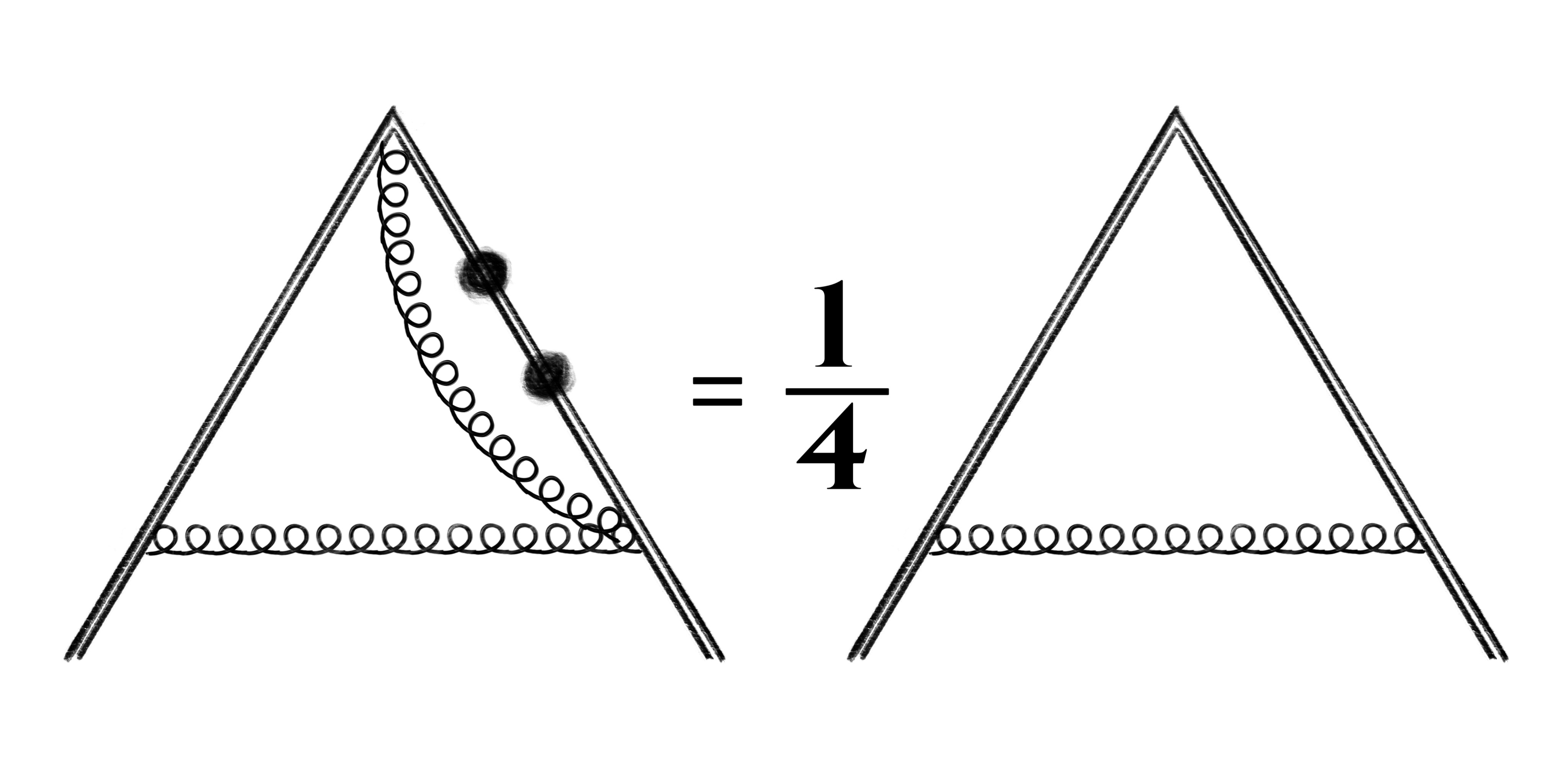
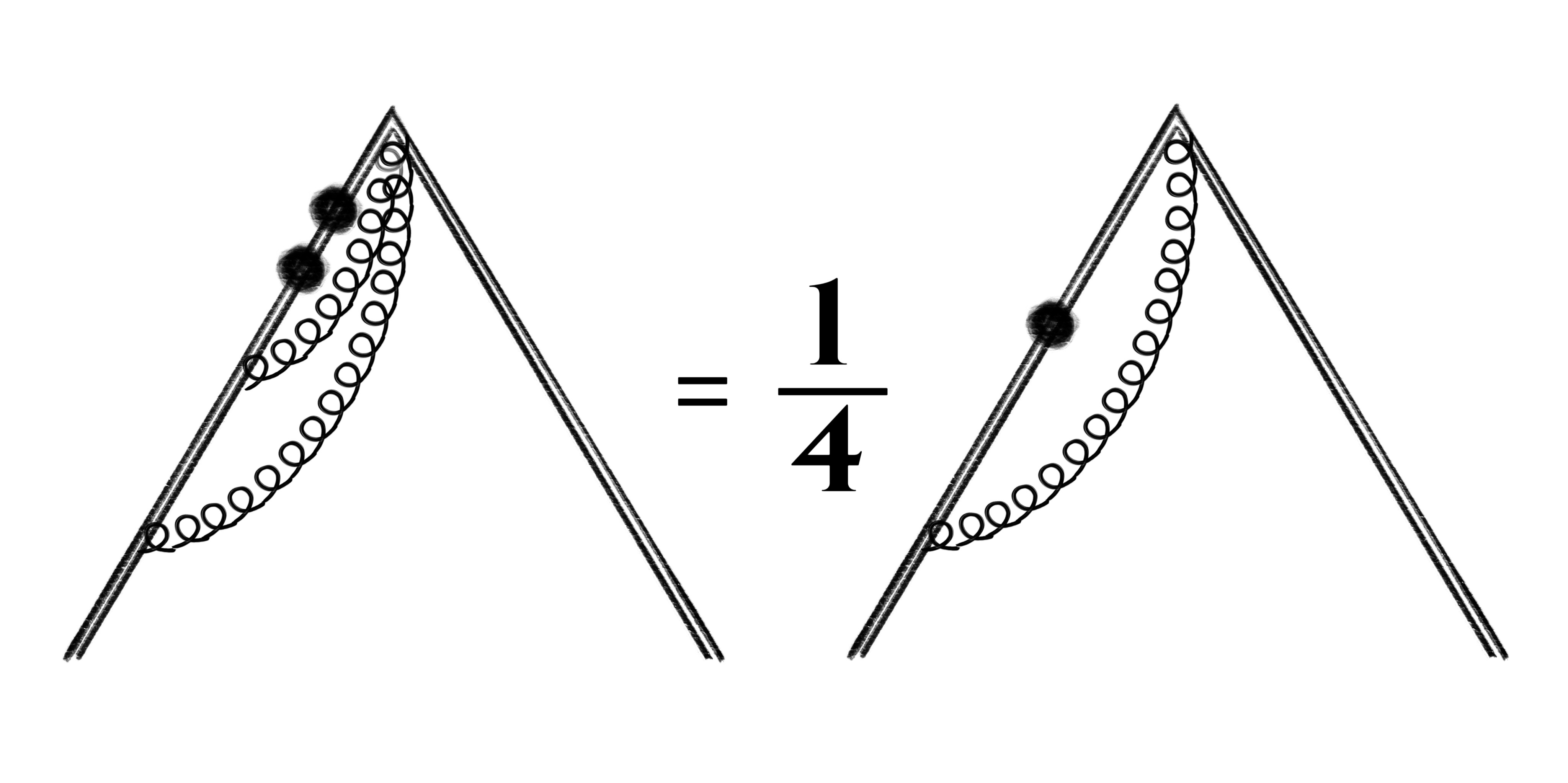
Figure 3: Relations between admissible integrals of different loop orders.

Another useful technique for generating linear relations for admissible integrals, is to integrate out bubble sub-diagrams. To be specific, for an $L$-loop HQET integral with the loop momenta $k_{1}$ only appearing in a bubble, with $a_{1}>2$,

$$\int\frac{d^{4-2\epsilon}k_{1}}{i\pi^{2-\epsilon}}\frac{1}{(-2k_{1}\cdot v_{1}+\delta)^{a_{1}}(-(k_{1}-k_{2})^{2})}=\frac{1}{(a_{1}-1)(a_{1}-2)}\frac{1}{(-2k_{2}v_{1}+\delta)^{a_{1}-2+2\epsilon}},\,.$$ (35)

Note that the new propagator’s index depends on $\epsilon$ which is not always desirable. However, for the $\epsilon^{-1}$ part only, as we show presently, the following replacement is valid, for $a_{1}>2$,

$$\int\frac{d^{4-2\epsilon}k_{1}}{i\pi^{2-\epsilon}}\frac{1}{(-2k_{1}\cdot v_{1}+\delta)^{a_{1}}(-(k_{1}-k_{2})^{2})}\to\frac{L-1}{L}\frac{1}{(a_{1}-1)(a_{1}-2)}\frac{1}{(-2k_{2}v_{1}+\delta)^{a_{1}-2}}\,.$$ (36)

The factor $(L-1)/L$ requires a comment. It takes into account the fact that the overall divergence we consider is computed from a volume integral, which in turn depends on the dimensionality, and hence the loop order. The factor compensates for the mismatch when comparing overall divergences of $L$ and $(L-1)$-loop integrals in dimensional regularization.

Applying this relation to the case of our family of crossed ladder integrals, we find the relations shown in Fig. 3.

3.3 Application to crossed ladder integrals

We construct IBP vectors, or equivalently differential operators as in eq. (32), which do not double propagators number five and six (see Fig. 2 and admissibility condition number 2 in subsection 2.3). We find that it suffices to consider those with the lowest scaling dimension in $\{k_{1},k_{2}\}$,

$${\bf P_{1}} =\partial_{1\mu}k_{1}^{\mu}\,,$$ (37)

$${\bf P_{2}} =\partial_{1\mu}k_{1\nu}v_{1}^{[\mu}v_{2}^{\nu]}\,,$$ (38)

$${\bf P_{3}} =(\partial_{1\mu}k_{1\mu}+\partial_{2\mu}k_{2\nu})v_{1}^{[\mu}v_{2}^{\nu]}\,.$$ (39)

In the top sector, the IBP relations,

$${\bf P_{2}}{\rm T^{(2)}}[1,1,1,1,1,1,0]=0\,,\quad{\bf P_{3}}{\rm T^{(2)}}[1,1,1,1,1,1,0]=0,$$ (40)

together with symmetry relations yield

$$0= A_{2}+B_{5}-2\,B_{1}-2(v_{1}\cdot v_{2})\,B_{2}\,,$$ (41)

$$0= A_{3}-A_{2}\,.$$ (42)

As a result, we keep only one master integral in the six-propagator sector, namely $A_{1}$, as $A_{2}$ and $A_{3}$ can be reduced to lower-sector integrals. It is possible to verify that finite integrals with two or more dots can be reduced in similar ways by applying the same set of IBP vectors on finite seeds which have more dots but fixed scaling dimension.

Let us now proceed with the five-propagator sectors. Using symmetry relations, together with the IBP identities

$${\bf P_{3}}{\rm T^{(2)}}[1,2,1,0,1,1,0]=0,\;\quad{\bf P_{3}}{\rm T^{(2)}}[1,1,2,0,1,1,0]=0,\;$$

$${\bf P_{1}}{\rm T^{(2)}}[1,2,0,1,1,1,0]=0,\;\quad{\bf P_{1}}{\rm T^{(2)}}[1,3,-1,1,1,1,0]=0,\;$$

$${\bf P_{1}}{\rm t^{(2)}}[2,2,-1,1,1,1,0,-1,0]=0,\;\quad{\bf P_{1}}{\rm t^{(2)}}[1,2,-1,2,1,1,0,0,-1]=0\,,$$ (43)

we find

$$0= B_{4}-2(v_{1}\cdot v_{2})B_{1}-B_{2}+2C_{4}\,,$$ (44)

$$0= B_{3}+B_{1}-2C_{1}\,,$$ (45)

$$0= B_{5}-2\,C_{1}\,,$$ (46)

$$0= 2\,B_{6}-C_{4}-3\,C_{2}\,,$$ (47)

$$0= B_{8}-2\,B_{6}+2\,C_{4}\,,$$ (48)

$$0= B_{7}-2\,C_{3}\,.$$ (49)

This allows us to eliminate $B_{3-8}$ in favor of $B_{1},B_{2}$ and integrals from lower sectors.

Next we move on to four-propagator integrals. Due to the presence of one-loop subdiagrams, they can be reduced to one-loop integrals, as shown in Fig. 3.

In summary, we find that the admissible crossed ladder integrals can be reduced to the following basis integrals:

$$\{A_{1},B_{1},B_{2},C_{1},C_{4}\}\,.$$ (50)

In the next section, we show how to compute these integrals from differential equations.

4 Algorithm for four-dimensional canonical differential equations

Having identified the IBP relations between admissible integrals, and hence a set of master integrals, we can now derive differential equations for the latter.

The HQET integrals we consider depend on a single variable $\phi$. It is convenient to trade the latter for another variable $x=\exp(i\phi)$ We may differentiate the master integrals with respect to $x$ by means of a differential operator acting on the integrand, e.g.

$${\bf d}\equiv\frac{x^{2}-1}{2}\frac{d}{dx}\equiv\frac{(v_{1}\cdot v_{2})v_{1}^{\mu}-v_{1}^{2}v_{2}^{\mu}}{\sqrt{v_{1}^{2}\,v_{2}^{2}}}\frac{\partial}{\partial v_{1}^{\mu}}\,.$$ (51)

Note that this operator does not double any gluon propagators and preserves the scaling dimension in each loop momenta. Thus for any admissible integral $f\in\mathbb{V}$, ${\bf d}f\in\mathbb{V}$. Given a basis of master integrals $\vec{f}$, one can write down a linear system of differential equations of degree $N={\rm dim}(\mathbb{V})$ :

$$\frac{d}{dx}\vec{f}=A(x)\vec{f}\,.$$ (52)

Let us illustrate how this works in the case of the crossed double ladder $A_{1}$. The crossed ladder integral family has a basis of five admissible master integrals

$$\vec{f}=\{A_{1}\,,B_{1}\,,B_{2}\,,C_{1}\,,C_{4}\}^{T}\,,$$ (53)

Let us now derive the differential equation that $A_{1}$ satisfies, and then determine it from now.

Taking the derivative of $A_{1}$ by means of the differential operator given in (51), we have

$${\bf{d}}A_{1}+2(v_{1}\cdot v_{2})A_{1}-A_{2}-B_{5}=0\,.$$ (54)

Taking into account eq.(41), this becomes

$$\frac{d}{dx}A_{1}=\frac{2(1+x^{2})}{x(1-x^{2})}A_{1}+\frac{4}{x^{2}-1}B_{1}+\frac{2(1+x^{2})}{x(x^{2}-1)}B_{2}\,.$$ (55)

One may iterate this procedure for $B_{1},B_{2}$, and then for $C_{1},C_{4}$. One finds that the integrals satisfy the differential equations (52) with

$${\mathbf{A}}=\frac{1+x^{2}}{1-x^{2}}\begin{pmatrix}\frac{2}{x}&-\frac{4}{1+x^{2}}&-\frac{2}{x}&0&0\\ 0&\frac{1}{x}&-\frac{2}{1+x^{2}}&0&0\\ 0&0&\frac{2}{x}&-\frac{4}{1+x^{2}}&0\\ 0&0&0&\frac{1}{x}&-\frac{2}{1+x^{2}}\\ 0&0&0&0&0\end{pmatrix}\,.$$ (56)

In order to solve this system of differential equations, it is useful to first simplify the equations, following Henn:2013pwa ; Caron-Huot:2014lda (see also Gehrmann:2014bfa ), or using the Initial algorithm Dlapa:2020cwj . The system above is of course very simple, so many different methods could be used. The key idea proposed in Henn:2013pwa is to convert the DE to a canonical form. The latter is obtained by choosing the basis integrals astutely. In fact, in order to find the transformation to a canonical form, under certain assumptions it is sufficient to choose one integral in a good way Dlapa:2020cwj . Here we can choose

$$F_{1}=\frac{1}{2}\left(x-\frac{1}{x}\right)^{2}A_{1}\,.$$ (57)

This choice can be justified by an integrand analysis Henn:2013pwa , as explained in detail in Grozin:2015kna . The factor ensures that $F_{1}$ has constant leading singularities.

Applying the Initial algorithm, we find that $F_{1}$ satisfies a fourth order Picard-Fuchs equation, which defines a rank-four canonical differential system

$$\frac{d}{dx}\begin{pmatrix}F_{1}\\ F_{2}\\ F_{3}\\ F_{4}\end{pmatrix}=\begin{pmatrix}0&\frac{2}{x}&0&0\\ 0&0&\frac{1+x^{2}}{x(1-x)(1+x)}&0\\ 0&0&0&\frac{4}{x}\\ 0&0&0&0\end{pmatrix}\begin{pmatrix}F_{1}\\ F_{2}\\ F_{3}\\ F_{4}\end{pmatrix}\,,$$ (58)

where

$$\{F_{1},F_{2},F_{3},F_{4}\}=\left\{\frac{(x^{2}-1)^{2}}{2\,x^{2}}A_{1},\frac{x^{2}-1}{x}\Big{(}B_{1}+\frac{1+x^{2}}{2\,x}B_{2}\Big{)},\frac{2(x^{2}-1)}{x}C_{1},C_{4}\right\}\,.$$ (59)

We see that eq. (58) is in canonical form. Moreover, the matrix is block triangular Caron-Huot:2014lda . This means that we can iteratively solve this equation. At each integration, there is one boundary constant to be fixed. The first integral, $F_{4}$, is constant, and we find its value by direct computation. The other boundary constants are fixed by observing that $F_{1},F_{2},F_{3}$ vanish at $x=1$. In this way, we find

$$F_{1}=\frac{1}{2}\left[\frac{1}{3}\ln^{3}x+\ln x\,{\rm Li}_{2}(x^{2})-{\rm Li}_{3}(x^{2})+\zeta_{2}\ln x+\zeta_{3}\right]\,.$$ (60)

This is in agreement with the known answer for $A_{1}$, see e.g. eq. (27) in Correa:2012nk .

This determines four of the five admissible master integrals. In case one wished to solve for the remaining one, one can do so by repeating the above steps with $F_{5}=\frac{1}{2}(x-1/x)^{2}B_{2}$ as the input to the Initial algorithm. In this case, one finds

$$\frac{d}{dx}\begin{pmatrix}F_{5}\\ F_{3}\\ F_{4}\end{pmatrix}=\begin{pmatrix}0&\frac{1}{x}&0\\ 0&0&\frac{4}{x}\\ 0&0&0\end{pmatrix}\begin{pmatrix}F_{5}\\ F_{3}\\ F_{4}\end{pmatrix}\,.$$ (61)

Solving this system, we find

$$F_{5}=\frac{1}{4}\ln^{2}x\,.$$ (62)

Hence we have found the complete basis of admissible UT integrals in the crossed ladder family.

5 Three-loop application

Here we apply our new four-dimensional method to three-loop integrals initially computed in Grozin:2014hna ; Grozin:2015kna . We find that in comparison, much fewer master integrals are needed, and the computation requires only a fraction of the computing time. For example, the standard differential equation approach for our three-loop HQET example via a publicly-available multiple-thread IBP solver took several hours, while our approach only took minutes with one core on the same machine.

The propagators of the three-loop integrals in Grozin:2015kna are,

$$D_{1}=-2k_{1}v_{1}+\delta\,,\quad D_{2}=-2k_{2}v_{1}+\delta\,,\quad D_{3}=-2k_{3}v_{1}+\delta\,,$$

$$D_{4}=-2k_{1}v_{2}+\delta\,,\quad D_{5}=-2k_{2}v_{2}+\delta\,,\quad D_{6}=-2k_{3}v_{2}+\delta\,,$$

$$D_{7}=-k_{1}^{2}\,,\quad D_{8}=-(k_{1}-k_{2})^{2}\,,\quad D_{9}=-(k_{2}-k_{3})^{2}\,,$$

$$D_{10}=-(k_{1}-k_{3})^{2}\,,\quad D_{11}=-k_{2}^{2}\,,\quad D_{12}=-k_{3}^{2}\,,$$ (63)

and the integral family is defined via

$$G[a_{1},\ldots,a_{12}]=\int\frac{d^{4-2\epsilon}k_{1}}{i\pi^{2-\epsilon}}\frac{d^{4-2\epsilon}k_{2}}{i\pi^{2-\epsilon}}\frac{d^{4-2\epsilon}k_{3}}{i\pi^{2-\epsilon}}\frac{1}{D_{1}^{a_{1}}\ldots D_{12}^{a_{12}}}\,.$$ (64)

For example, say, our goal is to calculate the $\epsilon^{-1}$ part of $G[1,1,0,0,1,1,1,1,1,0,0,1]$, which is an admissible integral (see Fig. 4). To set up a four-dimensional differential equation system, we first list four-dimensions IBPs for admissible integrals, as described in section 3, with a bound on the propagator indices. Besides the four-dimensional IBP relations, we also use the cross loop order relations introduced in the section 3. We find that some specific integrals in two sectors can be reduced to lower loop integrals.

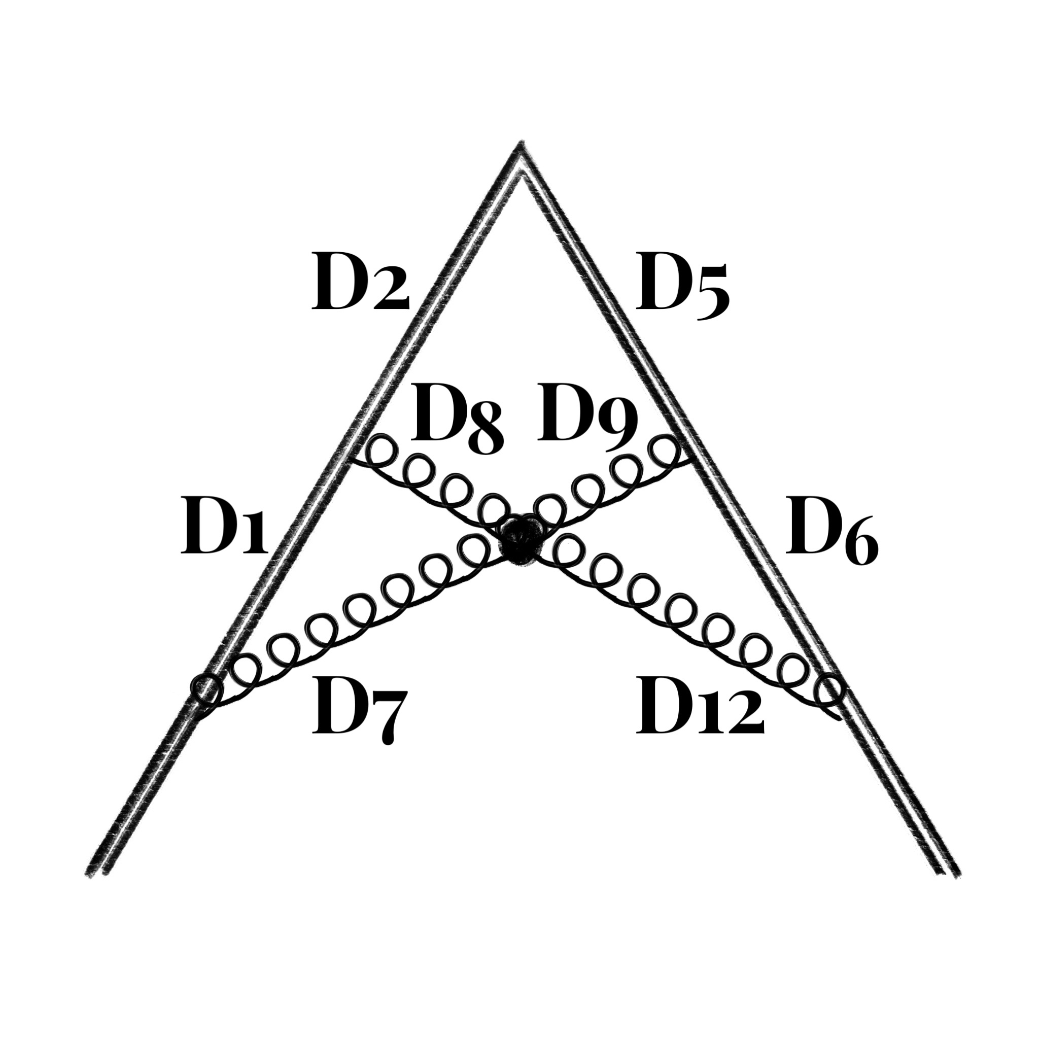
Figure 4: Three-loop HQET integral example

Combining the four-dimensional IBPs and cross loop-order relations, we get a linear system for the $\epsilon^{-1}$ part of the admissible integrals. This linear system is very sparse, free of the parameter $\epsilon$, and can be solved by FiniteFlow Peraro:2016wsq ; Peraro:2019svx in two minutes with one CPU core. We find $13$ irreducible integrals (cf. the auxiliary file “output/3lHQET_4D_MI.txt") that satisfy the differential equation,

$$\frac{d}{dx}\vec{I}=A(x)\vec{I}\,,$$ (65)

where $A$ is a $13\times 13$ matrix. The explicit expression of $A$ is given in the auxiliary file “output/3lHQET_4D_DE.txt".

A straightforward integrand analysis, as explained in detail in Grozin:2015kna , suggests that the integral

$$J_{1}\equiv\frac{(-1+x)(1+x)}{x}\ \lim_{\epsilon\to 0}\epsilon\,G[1,1,0,0,1,1,1,1,1,0,0,1]\,,$$ (66)

is UT and has constant leading singularity. This knowledge allows us to apply the INITIAL algorithm and find a basis of only $8$ UT integrals (in “output/3lHQET_4D_UT.txt"). They satisfy a simple canonical differential equations $\frac{d}{dx}\vec{J}=B\vec{J}$, where $B$ is an extremely sparse up-triangular matrix,

$$B \equiv\begin{pmatrix}0&-\frac{2}{(-1+x)(1+x)}&0&0&0&0&0&0\\ 0&0&\frac{1}{x}&0&0&0&0&0\\ 0&0&0&\frac{1}{x}&\frac{2x}{(-1+x)(1+x)}&0&0&0\\ 0&0&0&0&0&\frac{1}{x}&0&0\\ 0&0&0&0&0&0&\frac{1}{x}&0\\ 0&0&0&0&0&0&0&\frac{1}{x}\\ 0&0&0&0&0&0&0&-\frac{1}{x}\\ 0&0&0&0&0&0&0&0\end{pmatrix}\,,$$ (67)

Solving the differential equations and fixing the boundary constants, we find that there is degeneracy, and hence the dimension of the finite system is reduced to six. The solution for the top integral $J_{1}$ can be easily found as,

$$J_{1} =\frac{8}{3}H_{-1,-2,0,0}-\frac{8}{3}H_{-1,2,0,0}+\frac{8}{3}H_{1,-2,0,0}-\frac{8}{3}H_{1,2,0,0}-\frac{8}{3}H_{-1,0,0,0,0}-\frac{8}{3}H_{1,0,0,0,0}$$

$$-\zeta_{4}\,\ln(1-x)+\zeta_{4}\,\ln(1+x)+\frac{4}{3}\zeta_{3}\,\ln(1-x)\ln x-\frac{4}{3}\zeta_{3}\,\ln x\ln(1+x)$$

$$+\frac{8}{3}\zeta_{3}\,{\rm Li}_{2}(x)-\frac{2}{3}\zeta_{3}\,{\rm Li}_{2}(x^{2})\,.$$ (68)

where $H_{a_{1},\ldots,a_{n}}\equiv{\rm HPL}[\{a_{1},\ldots,a_{n}\},x]$ are the standard harmonic polylogarithms (HPLs). This analytic result is consistent with that in Grozin:2015kna .

It is interesting to compare our approach with that in the ref. Grozin:2015kna . In ref. Grozin:2015kna , in order to compute $J_{1}$, $39$ master integrals are needed. Here, in our approach, to get the $\epsilon^{-1}$ order of $J_{1}$, eventually we just need $6$ (or $13$) master integrals.

6 Summary and outlook

We presented a method for computing the leading divergent part of Feynman integrals that are free of subdivergences. Our method leverages simplifications that occur in limit as the dimensional regulator is taken to zero. We effectively use four-dimensional IBP relations and differential equations. This leads to substantial improvements: fewer master integrals are needed, and the IBP relations are faster to solve. The presented pedagogical examples and reproduced three-loop HQET integrals from the literature are proofs of concept. This method achieves the computation by the steps in Figure 5.

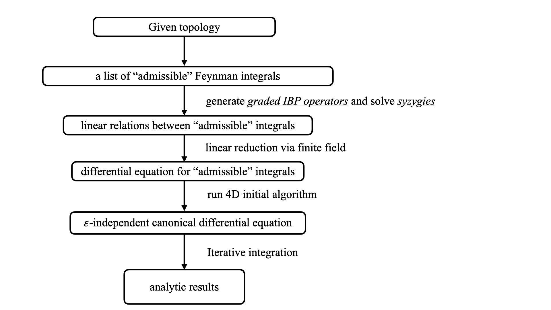
Figure 5: The algorithm flow chart of our method

We find the following extensions of the work in this paper promising:

1. Apply the method to cutting-edge applications that go beyond the state of the art. Potential applications include anomalous dimensions of composite operators, and the soft anomalous dimension matrix Liu:2022elt .

2. Extend the method to Feynman integrals with subdivergences, truncating the Laurent expansion in the dimensional regulator at a given order. This requires a careful identification of the relevant regions of loop integration. This will likely lead to an increase in the number of finite master integrals to be considered, but we still expect a significant simplification compared to the general, $D$-dimensional case.

3. Combine the method with insights into the structure of the Feynman graph polynomials from tropical geometry. The latter allow to identify the relevant divergent regions and to write their (finite) coefficients in terms of integrals that appear naturally from the geometry Schultka:2018nrs ; Arkani-Hamed:2022cqe .

References

- (1) V. A. Smirnov, Analytic tools for Feynman integrals, vol. 250. 2012, 10.1007/978-3-642-34886-0.
- (2) A. V. Kotikov, Differential equations method: New technique for massive Feynman diagrams calculation, Phys. Lett. B 254 (1991) 158.
- (3) Z. Bern, L. J. Dixon and D. A. Kosower, Dimensionally regulated one loop integrals, Phys. Lett. B 302 (1993) 299 [hep-ph/9212308].
- (4) E. Remiddi, Differential equations for Feynman graph amplitudes, Nuovo Cim. A 110 (1997) 1435 [hep-th/9711188].
- (5) T. Gehrmann and E. Remiddi, Differential equations for two loop four point functions, Nucl. Phys. B 580 (2000) 485 [hep-ph/9912329].
- (6) J. M. Henn, Multiloop integrals in dimensional regularization made simple, Phys. Rev. Lett. 110 (2013) 251601 [1304.1806].
- (7) S. Caron-Huot and J. M. Henn, Iterative structure of finite loop integrals, JHEP 06 (2014) 114 [1404.2922].
- (8) L. Tancredi, Integration by parts identities in integer numbers of dimensions. A criterion for decoupling systems of differential equations, Nucl. Phys. B 901 (2015) 282 [1509.03330].
- (9) A. Connes and D. Kreimer, Hopf algebras, renormalization and noncommutative geometry, Commun. Math. Phys. 199 (1998) 203 [hep-th/9808042].
- (10) S. Catani and M. H. Seymour, A General algorithm for calculating jet cross-sections in NLO QCD, Nucl. Phys. B 485 (1997) 291 [hep-ph/9605323].
- (11) L. J. Dixon, L. Magnea and G. F. Sterman, Universal structure of subleading infrared poles in gauge theory amplitudes, JHEP 08 (2008) 022 [0805.3515].
- (12) O. Almelid, C. Duhr and E. Gardi, Three-loop corrections to the soft anomalous dimension in multileg scattering, Phys. Rev. Lett. 117 (2016) 172002 [1507.00047].
- (13) C. Anastasiou and G. Sterman, Removing infrared divergences from two-loop integrals, JHEP 07 (2019) 056 [1812.03753].
- (14) J. Gluza, K. Kajda and D. A. Kosower, Towards a Basis for Planar Two-Loop Integrals, Phys. Rev. D 83 (2011) 045012 [1009.0472].
- (15) R. M. Schabinger, A New Algorithm For The Generation Of Unitarity-Compatible Integration By Parts Relations, JHEP 01 (2012) 077 [1111.4220].
- (16) C. Dlapa, J. Henn and K. Yan, Deriving canonical differential equations for Feynman integrals from a single uniform weight integral, JHEP 05 (2020) 025 [2002.02340].
- (17) A. Grozin, J. M. Henn, G. P. Korchemsky and P. Marquard, The three-loop cusp anomalous dimension in QCD and its supersymmetric extensions, JHEP 01 (2016) 140 [1510.07803].
- (18) A. M. Polyakov, Gauge Fields as Rings of Glue, Nucl. Phys. B 164 (1980) 171.
- (19) R. A. Brandt, F. Neri and M.-a. Sato, Renormalization of Loop Functions for All Loops, Phys. Rev. D 24 (1981) 879.
- (20) G. P. Korchemsky and A. V. Radyushkin, Renormalization of the Wilson Loops Beyond the Leading Order, Nucl. Phys. B 283 (1987) 342.
- (21) A. G. Grozin, Heavy quark effective theory, Springer Tracts Mod. Phys. 201 (2004) 1.
- (22) J. Frenkel and J. C. Taylor, Non-Abelian Eikonal Exponentiation, Nucl. Phys. B 246 (1984) 231.
- (23) J. G. M. Gatheral, Exponentiation of Eikonal Cross-sections in Nonabelian Gauge Theories, Phys. Lett. B 133 (1983) 90.
- (24) R. N. Lee, Presenting LiteRed: a tool for the Loop InTEgrals REDuction, 1212.2685.
- (25) R. N. Lee, Reducing differential equations for multiloop master integrals, JHEP 04 (2015) 108 [1411.0911].
- (26) A. Pak, The Toolbox of modern multi-loop calculations: novel analytic and semi-analytic techniques, J. Phys. Conf. Ser. 368 (2012) 012049 [1111.0868].
- (27) K. J. Larsen and Y. Zhang, Integration-by-parts reductions from unitarity cuts and algebraic geometry, Phys. Rev. D93 (2016) 041701 [1511.01071].
- (28) J. Böhm, A. Georgoudis, K. J. Larsen, M. Schulze and Y. Zhang, Complete sets of logarithmic vector fields for integration-by-parts identities of Feynman integrals, Phys. Rev. D98 (2018) 025023 [1712.09737].
- (29) J. Böhm, A. Georgoudis, K. J. Larsen, H. Schönemann and Y. Zhang, Complete integration-by-parts reductions of the non-planar hexagon-box via module intersections, JHEP 09 (2018) 024 [1805.01873].
- (30) D. Bendle, J. Böhm, W. Decker, A. Georgoudis, F.-J. Pfreundt, M. Rahn et al., Integration-by-parts reductions of Feynman integrals using Singular and GPI-Space, JHEP 02 (2020) 079 [1908.04301].
- (31) Z. Wu, J. Böhm, R. Ma, H. Xu and Y. Zhang, “NeatIBP 1.0 — A package generating small-size integration-by-parts relations for feynman integrals.” https://github.com/yzhphy/NeatIBP, 2023.
- (32) C. Bouillaguet, “SpaSM: a sparse direct solver modulo .” http://github.com/cbouilla/spasm, 2017.
- (33) T. Gehrmann, A. von Manteuffel, L. Tancredi and E. Weihs, The two-loop master integrals for , JHEP 06 (2014) 032 [1404.4853].
- (34) D. Correa, J. Henn, J. Maldacena and A. Sever, The cusp anomalous dimension at three loops and beyond, JHEP 05 (2012) 098 [1203.1019].
- (35) A. Grozin, J. M. Henn, G. P. Korchemsky and P. Marquard, Three Loop Cusp Anomalous Dimension in QCD, Phys. Rev. Lett. 114 (2015) 062006 [1409.0023].
- (36) T. Peraro, Scattering amplitudes over finite fields and multivariate functional reconstruction, JHEP 12 (2016) 030 [1608.01902].
- (37) T. Peraro, FiniteFlow: multivariate functional reconstruction using finite fields and dataflow graphs, JHEP 07 (2019) 031 [1905.08019].
- (38) Z. L. Liu and N. Schalch, Infrared singularities of multi-leg QCD amplitudes with a massive parton at three loops, 2207.02864.
- (39) K. Schultka, Toric geometry and regularization of Feynman integrals, 1806.01086.
- (40) N. Arkani-Hamed, A. Hillman and S. Mizera, Feynman Polytopes and the Tropical Geometry of UV and IR Divergences, 2202.12296.