RUP-22-25
KEK-TH-2365
KEK-Cosmo-0280
KEK-QUP-2022-0011
YITP-22-143
CTPU-PTC-22-27

Threshold of Primordial Black Hole Formation against
Velocity Dispersion in Matter-Dominated Era

Tomohiro Harada^a, Kazunori Kohri^b,c,d,e, Misao Sasaki^e,f,g,

Takahiro Terada^h, and Chul-Moon Yooⁱ

^a   Department of Physics, Rikkyo University, Toshima, Tokyo 171-8501, Japan
^b   Institute of Particle and Nuclear Studies, KEK, 1-1 Oho, Tsukuba, Ibaraki 305-0801, Japan
^c   International Center for Quantum-field Measurement Systems for Studies of the Universe and Particles (QUP, WPI), KEK, 1-1 Oho, Tsukuba, Ibaraki 305-0801, Japan
^d  The Graduate University for Advanced Studies (SOKENDAI),
1-1 Oho, Tsukuba, Ibaraki 305-0801, Japan
^e  Kavli Institute for the Physics and Mathematics of the Universe (WPI),
University of Tokyo, Kashiwa 277-8583, Japan
^f  Center for Gravitational Physics, Yukawa Institute for Theoretical Physics,
Kyoto University, Kyoto 606-8502, Japan
^g  Leung Center for Cosmology and Particle Astrophysics,
National Taiwan University, Taipei 10617, Taiwan
^h  Center for Theoretical Physics of the Universe,
Institute for Basic Science (IBS), Daejeon, 34126, Korea
ⁱ  Division of Particle and Astrophysical Science, Graduate School of Science,
Nagoya University, Nagoya 464-8602, Japan

We study the effects of velocity dispersion on the formation of primordial black holes (PBHs) in a matter-dominated era. The velocity dispersion is generated through the nonlinear growth of perturbations and has the potential to impede the gravitational collapse and thereby the formation of PBHs. To make discussions clear, we consider two distinct length scales. The larger one is where gravitational collapse occurs which could lead to PBH formation, and the smaller one is where the velocity dispersion develops due to nonlinear interactions. We estimate the effect of the velocity dispersion on the PBH formation by comparing the free-fall timescale and the timescale for a particle to cross the collapsing region. As a demonstration, we consider a log-normal power spectrum for the initial density perturbation with the peak value $\sigma_{0}^{2}$ at a scale that corresponds to the larger scale. We find that the threshold value of the density perturbation $\tilde{\delta}_{\rm th}$ at the horizon entry for the PBH formation scales as $\tilde{\delta}_{\rm th}\propto\sigma_{0}^{2/5}$ for $\sigma_{0}\ll 1$.

1 Introduction

Black holes are widely accepted to exist in the Universe through various observations such as the motion of surrounding celestial objects [1, 2, 3, 4], gravitational-wave signals from binary-black-hole mergers [5, 6, 7], and the black hole shadow [8]. Some of the black holes might have a primordial origin [9, 10, 11]. Depending on their mass, primordial black holes (PBHs) may explain dark matter abundance [12, 13, 14, 15], the binary black hole abundance observed by the gravitational-wave events [16, 17, 18, 19], an excess of microlensing events [20], a potential gravitational-wave signal at a pulsar timing array [21, 22, 23, 24, 25, 26, 27], the seeds of supermassive black holes and cosmic structures [28, 29, 30, 31, 32, 33, 34]. PBHs whose lifetime is shorter than the age of the Universe may also play important roles in the early Universe such as baryogenesis [35, 36, 37] and the production of stochastic gravitational-wave background [38, 39, 40, 41, 42, 43, 44, 45].

For any applications of PBHs, their abundance is a basic quantity that determines their cosmological significance. For the estimation of the abundance in a radiation-dominated (RD) era, three tools conventionally adopted are: the criterion of PBH formation [56, 57, 58, 59, 60, 61, 62, 63, 64, 65, 66, 67, 68], the peaks theory for the statistical treatment of the initial profiles [69, 70, 71, 72], and the critical behavior of the PBH formation [73, 74, 75, 76] for sufficiently spherical collapses. The latest theoretical estimation of the PBH abundance for the monochromatic curvature power spectrum can be seen in Ref. [77] for Gaussian and local-type non-Gaussian curvature perturbations (see also Refs. [78, 79, 80, 77, 81] for effects of the non-Gaussianity), where the PBH mass function is calculated based on an approximately universal criterion [65] and the peaks theory [72].

In a matter-dominated (MD) era, since the pressure of the fluid, which is the most effective factor to impede PBH formation in an RD era, is absent and the criterion of PBH formation obtained with the fluid approximation does not apply. The absence of the pressure would make the gravitational collapse easier, and lower peaks of the density perturbation may contribute to PBH abundance [82, 83]. However, the high-peak approximation in peaks theory becomes worse and the spherical symmetry assumption, which is relevant to rare high peaks [69], may not be accurate. Furthermore, it is well known that the deviation from the spherical symmetry can significantly grow in the gravitational collapse in the case of pressureless matter [84, 85]. Thus, non-spherical initial profiles are inevitable, and they may lead to the complicated nonlinear dynamics associated with deformation and rotation. In addition, the pressureless fluid approximation breaks down as soon as nonlinearity becomes important due to the occurrence of shell-crossing singularities. In reality, the pressureless matter obeys the collisionless Boltzmann equation, and velocity dispersion will develop in the nonlinear regime. Thus, careful studies that take account of various effects are required in order to understand the PBH formation in an MD era. There are several analytical studies in the literature, in which the effects of asphericity [86], angular momentum [87], and inhomogeneity [82, 83, 88], were estimated under some assumptions and approximations. For an analysis in numerical relativity, see Ref. [89].

In this paper, we consider the effect of the velocity dispersion inside the collapsing region and discuss the conditions for the velocity dispersion to impede the PBH formation in the MD era. To make discussions simple and clear, we consider two distinct length scales. The larger one is where gravitational collapse occurs which could lead to PBH formation, and the smaller one is where the velocity dispersion develops due to nonlinear interactions. The paper is organized as follows. In Sec. 2, we overview the situation we consider by describing our setup and assumptions. In Sec. 3, we derive the conditions for the velocity dispersion to impede the PBH formation. In doing so, we find there are essentially two different scenarios, depending on when the velocity dispersion emerges, details of which are discussed in Appendix A. In Sec. 4, the conditions to impede the PBH formation are rephrased in terms of the density threshold for the PBH formation for a given density power spectrum. In Sec. 5, using the obtained results, we compute the PBH production probability as a function of the peak amplitude of the power spectrum of the density perturbation. Our conclusions are given in Sec. 6. Throughout this paper, we use the units in which both the speed of light and Newton’s gravitational constant are unity, $G=c=1$.

2 Overview

To avoid any confusion in understanding how the velocity dispersion is generated and works as a preventing factor against PBH formation, before discussing the details, let us clarify our setup and assumptions.

First, the rough basic picture is as follows. We consider a high-density region of the comoving scale $k_{\mathrm{PBH}}$ that undergoes gravitationally collapse and may lead to PBH formation, which may be impeded by the velocity dispersion generated by the dynamics on a scale $k$ where $k>k_{\mathrm{PBH}}$. Here we suppose that a finite power of perturbation also exists on these small scales. When the perturbations on the small scales enter the nonlinear regime, that is, when the density perturbation becomes high enough to render the fluid approximation invalid, the velocity dispersion is assumed to be generated, so that the random motion of the constituent particles can act against gravity. In this phase, if the repulsive effect due to this generated random motion dominates the dynamics of the whole system over the length scale $1/k_{\text{PBH}}$, the collapsing region will be eventually virialized, so that the PBH formation will be impeded. Here, we note that the velocity dispersion may get effective on the scale $k_{\mathrm{PBH}}$ not immediately after it is generated on the scale $k$ but later, depending on its magnitude. We describe more specific scenarios in the following setup and assumptions.

Now let us describe the setup and assumptions.

• We consider only the two separated comoving scales characterized by $k$ and $k_{\rm PBH}$. We call $k_{\rm PBH}$ the large or PBH scale, while $k$ the small scale. Throughout this paper, the tilded quantities are those for the PBH scale $k_{\rm PBH}$, while those for the small scale $k$ are not tilded. Thus in particular $\tilde{k}\equiv k_{\rm PBH}$. Two exceptions are the velocity dispersion $\sigma_{v}(t)$ as a function of time, and the root-mean-square amplitude of the density perturbation at the horizon entry $\sigma_{\delta,{\rm ent}}(k)$ as a function of the comoving wavenumber.

• Since we discuss a cosmological patch that is going to form a PBH (or to be impeded by the velocity dispersion), the density perturbation on this patch $\tilde{\delta}_{\rm ent}$ is exceptionally higher than the typical amplitude, $\tilde{\delta}_{\rm ent}\gg\sigma_{\delta,{\rm ent}}(\tilde{k})$, at the time the scale enters the Hubble horizon.

• On the other hand, we suppose the amplitude of the smaller-scale perturbations is given by a typical value, that is, the amplitude at the horizon entry $\delta_{\rm ent}(k)$ is typically given by the standard deviation of the density perturbation, $|\delta_{\rm ent}(k)|=\mathcal{O}(\sigma_{\delta,{\rm ent}}(k))$. This magnitude is also assumed to be so small that the PBH formation on the small scale is negligible. Then, except for Sec. 5, we assume for simplicity that the only impeding factor against PBH formation on the scale $\tilde{k}$ is the velocity dispersion. In addition to the velocity dispersion, other potential impeding factors against the PBH formation will be briefly discussed in Sec. 5.

• We assume that the fluid approximation (i.e., coherent flow of particles with negligible velocity dispersion) is valid on the scale $k$ until caustics appear, that is, until the perturbation enters the nonlinear regime (provided that larger scales have not yet collapsed). The collapsing overdense regions may be locally described by the closed Friedmann-Lemaître-Robertson-Walker (FLRW) universe models (see, e.g., Ref. [91]). Then the collapsing time on the PBH scale $\tilde{k}$ and that on the scale $k$ may be estimated by using the closed FLRW collapsing model, which we denote by $\tilde{t}_{\mathrm{coll}}$ and $t_{\mathrm{coll}}$, respectively. It should be noted that, if $t_{\mathrm{coll}}\gtrsim\tilde{t}_{\mathrm{coll}}$, the smaller-scale perturbations cannot be independent of the surrounding over-density associated with the PBH scale. Namely, the actual collapsing time will be earlier than $t_{\rm coll}$ in that case.

It should be noted that the velocity dispersion generated on the scale $k$ may not be immediately shared with the whole region on the scale $\tilde{k}$. If the virialization is completed on the smaller scale before the collapse of the larger scale, the matter is confined in the virialized halos. In this case, the halos behave as macroscopic self-gravitating comoving particles, hence no impeding effect due to the velocity dispersion is expected against the gravitational collapse on the scale $k_{\mathrm{PBH}}$. Therefore, we consider the two possible scenarios: Case I and Case II as follows.

• Case I: We assume the virialization of the perturbations on the smaller scale is completed before the collapse of the larger scale, i.e., $t_{\mathrm{vir}}<\tilde{t}_{\mathrm{coll}}$. In this case, the velocity dispersion is released when the mean density on the scale $\tilde{k}$ becomes comparable to the density of a halo. At this point, the halos dissolve into ambient space. We identify the time when the halos dissolve with the time ($\equiv t_{*}$) at which the velocity dispersion becomes effective on the PBH scale $\tilde{k}$.

• Case II: We assume $t_{\rm vir}>\tilde{t}_{\rm coll}$, i.e., there is no time for the small scale to collapse and form virialized halos. In this case, the velocity dispersion is directly released soon after the smaller-scale perturbations grow into the nonlinear regime. Since the evolution of the small-scale perturbations should be necessarily promoted (especially in case II) by the evolution of the surrounding high-density region on the scale $1/\tilde{k}$, we will consider the linear density perturbation $\delta_{\rm com}$ in a FLRW universe in the synchronous comoving gauge for the evolution of the small-scale perturbations. Then, the time $t_{*}$ when the velocity dispersion becomes effective on the scale $\tilde{k}$ is identified with the time when $\delta_{\rm com}\sim 1$, i.e., when caustics appear.

The detailed derivation of the criterion that distinguishes the two cases is given in Appendix. Here let us briefly present an order-of-magnitude estimate. Consider a region where a positive density perturbation $\tilde{\delta}$ exists. In a linear regime, it grows in proportion to the scale factor $a$ at a matter-dominated stage, where $a\propto t^{2/3}$. Thus $\tilde{\delta}(t)=(t/\tilde{t}_{\rm ent})^{2/3}\tilde{\delta}_{\rm ent}$, where $\tilde{\delta}_{\rm ent}$ is the amplitude of the density perturbation at horizon entry. The time at which the region collapses is sometime after the amplitude reached $\mathcal{O}(1)$. Ignoring order-of-unity numerical factors, we may identify the time when $\tilde{\delta}=1$ as the collapse time, $\tilde{t}_{\rm col}$. When the region collapses but doesn’t lead to the formation of a black hole, the system virializes approximately at the same time, $\tilde{t}_{\rm vir}\sim\tilde{t}_{\rm col}$. Since the same argument applies to the small scale, the region of the small scale will be virialized, as $\delta_{\rm ent}$ is assumed to be very small. Thus we have

$${t}_{\rm vir}\sim{t}_{\rm ent}{\delta}_{\rm ent}^{-3/2}\,.$$ (1)

On the other hand, on the PBH scale $\tilde{k}$, the region may form a black hole if there is no impeding factors. So we estimate the collapse time as

$$\tilde{t}_{\rm col}\sim\tilde{t}_{\rm ent}\tilde{\delta}_{\rm ent}^{-3/2}\,.$$ (2)

Now recalling that the comoving scale $k$ may be expressed in terms of its horizon entry time as $k=(aH)_{\rm ent}\propto t_{\rm ent}^{-1/3}$, one finds

$$\left(\frac{{t}_{\rm vir}}{\tilde{t}_{\rm col}}\right)^{2/3}\sim\left(\frac{{t}_{\rm ent}}{\tilde{t}_{\rm ent}}\right)^{2/3}\frac{\tilde{\delta}_{\rm ent}}{\delta_{\rm ent}}=\frac{\tilde{k}^{2}}{{k}^{2}}\frac{\tilde{\delta}_{\rm ent}}{\delta_{\rm ent}}\,.$$ (3)

Thus the criterion is

$${\rm Case~{}I} :~{}{t}_{\mathrm{vir}}<\tilde{t}_{\mathrm{coll}}\quad\Leftrightarrow\quad{k}^{2}\delta_{\rm ent}>\tilde{k}^{2}\tilde{\delta}_{\rm ent}\,,$$

$${\rm Case~{}II} :~{}{t}_{\mathrm{vir}}>\tilde{t}_{\mathrm{coll}}\quad\Leftrightarrow\quad{k}^{2}\delta_{\rm ent}<\tilde{k}^{2}\tilde{\delta}_{\rm ent}\,.$$ (4)

In both cases, once the velocity dispersion is shared over the whole patch of the PBH scale at $t=t_{*}$, the criterion for the PBH formation can be roughly evaluated by comparing the gravitational free-fall time $\Delta\tilde{t}_{\rm ff}\propto\tilde{\rho}^{-1/2}\propto\tilde{R}^{3/2}$ with the sound-wave crossing time $\Delta\tilde{t}_{\rm cross}\sim\tilde{R}/\sigma_{v}$, where $\tilde{\rho}$, $\tilde{R}$, and $\sigma_{v}$ are the density, the physical size of the scale $\tilde{k}$, and the velocity dispersion, respectively. As the velocity dispersion increases, the crossing time becomes shorter, and the PBH formation is eventually impeded. The evaluation of the PBH formation condition is given in Sec. 3.

In Sec. 4, assuming that the scale $k$ can be treated independently of the scale $\tilde{k}$, we consider a log-normal density spectrum $\ln\sigma(k)=\ln\sigma_{0}-\mu\ln(k/\tilde{k})^{2}$, where $\sigma_{0}$ and $\mu$ are dimensionless parameters, and evaluate the threshold amplitude of the density perturbation at horizon entry $\tilde{\delta}_{\rm ent}$. In Sec. 5, the PBH production rate is roughly evaluated following the procedure provided in Ref. [87], and the effect of the velocity dispersion is compared with the spin effects reported in Ref. [87].

3 Effect of the Velocity Dispersion against Collapse

The velocity dispersion may impede the gravitational collapse after the velocity dispersion is shared in the whole region of the PBH scale $\tilde{k}$. First, let us evaluate the impeding effect of the uniformly distributed velocity dispersion. We consider a spherical ball on the PBH scale. Once the velocity dispersion is shared over the collapsing ball, the velocity dispersion simply increases as $\sigma_{v}\propto\tilde{\rho}^{1/3}$ as the system collapses adiabatically, according to Liouville’s theorem. More explicitly, we have

$$\sigma_{v}(t)= \sigma_{v}(t_{*})\left(\frac{\tilde{\rho}(t)}{\tilde{\rho}(t_{*})}\right)^{1/3}=\sigma_{v}(t_{*})\frac{\tilde{R}(t_{*})}{\tilde{R}(t)},$$ (5)

where $t_{*}<t$ and $t_{*}$ is the time when the velocity dispersion is shared over the whole collapsing region.

The sound-wave crossing time across the region of the size $R(t)$ is estimated as

$$\Delta\tilde{t}_{\text{cross}}\simeq \frac{\tilde{R}(t)}{\sigma_{v}(t)}=\frac{3}{2\sigma_{v}(t_{*})}\frac{\tilde{R}(t)^{2}}{\tilde{R}(t_{*})\tilde{R}_{\rm ent}}\tilde{t}_{\rm ent},$$ (6)

where $\tilde{R}_{\rm ent}$ is the radius at the horizon entry time $\tilde{t}_{\rm ent}$ satisfying $\tilde{R}_{\rm ent}=1/\tilde{H}_{\rm ent}=3\tilde{t}_{\rm ent}/2$ in the Einstein-de Sitter background with $\tilde{H}_{\rm ent}$ being the Hubble parameter at the horizon entry. On the other hand, the free-fall time is estimated as

$$\Delta\tilde{t}_{\text{ff}}\simeq\left(\frac{\tilde{R}(t)}{\tilde{R}_{\text{ent}}}\right)^{3/2}\tilde{t}_{\text{ent}}.$$ (7)

Noting that $\Delta\tilde{t}_{\rm cross}\propto\tilde{R}^{2}$ and $\Delta\tilde{t}_{\rm ff}\propto\tilde{R}^{3/2}$, and $\Delta\tilde{t}_{\rm cross}>\Delta\tilde{t}_{\rm ff}$ at the time of horizon entry, the collapse halts when $\Delta\tilde{t}_{\rm ff}=\Delta\tilde{t}_{\rm cross}$ if the radius is larger than the Schwarzschild radius at that time. Let us denote the value of $\tilde{R}(t)$ at $\Delta\tilde{t}_{\rm ff}(t)=\Delta\tilde{t}_{\rm cross}(t)$ by $\tilde{R}_{\rm halt}$. We find

$$\tilde{R}_{\rm halt}=\frac{4}{9}\sigma_{v}^{2}(t_{*})\frac{\tilde{R}^{2}(t_{*})}{\tilde{R}_{\rm ent}^{2}}\tilde{R}_{\rm ent}\,.$$ (8)

If this is larger than $2\tilde{M}$, i.e., $\tilde{R}_{\rm halt}>\tilde{R}_{\rm ent}=1/\tilde{H}_{\rm ent}=2\tilde{M}$, the collapse halts before the PBH formation. Conversely, a PBH forms if $\tilde{R}_{\rm halt}<2\tilde{M}$. Thus, the condition for the PBH non-formation can be rewritten in the following simple form.

$$\sigma_{v}(t_{*})\tilde{R}(t_{*})>\frac{3}{2}\tilde{R}_{\rm ent}.$$ (9)

To understand how the velocity dispersion is shared over the whole region of the size $1/\tilde{k}$, we introduce a closed FLRW collapsing model and consider its perturbations as given in Appendix A. Deferring detailed explanations of the complicated manipulations, here we just refer to the results. According to the discussion in Appendix A, depending on whether the halo formation on the scale $k$ can be completed before the collapse of the scale $\tilde{k}$, we can rewrite Eq. (9), i.e., PBH non-formation condition, as

$$\delta_{\rm ent}<\frac{\tilde{k}^{4}}{k^{4}} \text{for }~{}\text{Case I~{}: }\quad k^{2}\delta_{\rm ent}>\tilde{k}^{2}\tilde{\delta}_{\rm ent}\,,$$ (10)

$$\delta_{\rm ent}>\frac{k}{\tilde{k}}\tilde{\delta}_{\rm ent}^{5/2} \text{for }~{}\text{Case II: }\quad k^{2}\delta_{\rm ent}<\tilde{k}^{2}\tilde{\delta}_{\rm ent}\,,$$ (11)

where we have ignored factors of order unity. The qualitative features of the above conditions can be understood as follows.

For Case I, the virialization of the scale $k$ occurs before the collapse of the would-be PBH scale. The condition (10) is a bit counter-intuitive. So let us see why it is the case. Since the gravitational potential $\Psi$ is constant in time in the matter-dominated universe, and $\delta_{\rm ent}\sim\Psi$ at horizon crossing, the virial velocity dispersion is estimated as $\sigma_{v}^{2}\sim\Psi\sim\delta_{\rm ent}$ (see Eq. (43)). The virial density is $\rho_{\rm vir}=\rho_{\rm ent}(a_{\rm ent}/a_{\rm vir})^{3}=\rho_{\rm ent}(\delta_{\rm ent}/\delta_{\rm vir})^{3}\sim\rho_{\rm ent}\delta_{\rm ent}^{3}$ since $\delta\propto a$ and $\delta_{\rm vir}=O(1)$. As the collapse of a ball of the scale $\tilde{k}$ proceeds, the density $\tilde{\rho}$ reaches $\rho_{\rm vir}$ at $t=t_{*}$, and the velocity dispersion is released to the entire ball, i.e., $\tilde{\rho}(t_{*})=\rho_{\rm vir}$. Hence we obtain the relation,

$$\delta_{\rm ent} \sim \left(\dfrac{\rho_{\rm vir}}{\rho_{\rm ent}}\right)^{1/3}=\left(\dfrac{\rho_{\rm vir}}{\tilde{\rho}_{\rm ent}}\right)^{1/3}\left(\dfrac{\tilde{\rho}_{\rm ent}}{\rho_{\rm ent}}\right)^{1/3}=\left(\dfrac{\tilde{\rho}(t_{*})}{\tilde{\rho}_{\rm ent}}\right)^{1/3}\left(\dfrac{a_{\rm ent}}{\tilde{a}_{\rm ent}}\right)$$ (12)

$$= \dfrac{\tilde{R}_{\rm ent}}{\tilde{R}(t_{*})}\dfrac{\tilde{k}^{2}}{k^{2}}\,.$$

Recalling that $\delta_{\rm ent}\sim\sigma_{v}^{2}$ (Eq. (43)), this implies

$$\sigma_{v}^{2}\dfrac{\tilde{R}(t_{*})^{2}}{\tilde{R}_{\rm ent}^{2}}\sim\delta_{\rm ent}\times\dfrac{\tilde{k}^{4}}{k^{4}}\frac{1}{\delta_{\rm ent}^{2}}=\dfrac{\tilde{k}^{4}}{k^{4}}\frac{1}{\delta_{\rm ent}}\,.$$ (13)

With Eq. (9), this gives the condition quoted in Eq. (10). Here we have ignored all the coefficients of $\mathcal{O}(1)$. As one can see from the above estimate, the reason why the condition gives an upper bound on $\delta_{\rm ent}$ is because it would make the small-scale virialized halos so small and dense that the large-scale region would collapse to a black hole before the velocity dispersion is shared over the entire region of the PBH scale $\tilde{k}$. More details are given in Appendix A.3.

Let us now turn to Case II where the velocity dispersion is shared by the whole PBH region before the perturbations on the small scale $k$ are virialized. The analysis in this case is a bit more complicated as one has to consider the growth of the small-scale perturbation in the collapsing region of the scale $\tilde{k}$. The detailed derivation of the condition (11) is defered to Appendix A.4. Here we only mention that the reason why it depends on $\tilde{\delta}_{\mathrm{ent}}$ is precisely because of this fact that the small-scale perturbation grows within the collapsing ball of the large scale. The reason why the condition gives a lower bound on $\delta_{\mathrm{ent}}$ is simply because a larger $\delta_{\mathrm{ent}}$ gives a larger velocity dispersion, and hence it is easier to impede the PBH formation.

4 Threshold of the Density Perturbation

As the effect of the perturbation on the small scale $k$ is statistical, hereafter, we replace $\delta_{\rm ent}$ by its root-mean-square value $\sigma_{\delta,{\rm ent}}(k)$. Then, the condition for impeding the PBH formation due to velocity dispersion can be summarized as follows:

$$\sigma_{\delta,\rm ent}(k)<\left(\frac{k}{\tilde{k}}\right)^{-4} \text{for }~{}\text{Case I~{}:}\quad\sigma_{\delta,{\rm ent}}(k)>\tilde{\delta}_{\rm ent}\left(\frac{k}{\tilde{k}}\right)^{-2},$$ (14)

$$\sigma_{\delta,{\rm ent}}(k)>\tilde{\delta}_{\rm ent}^{5/2}\left(\frac{k}{\tilde{k}}\right) \text{for }~{}\text{Case II:}\quad\sigma_{\delta,{\rm ent}}(k)<\tilde{\delta}_{\rm ent}\left(\frac{k}{\tilde{k}}\right)^{-2},$$ (15)

where we remind that the tilded quantities are those associated with the PBH scale. So only the range $k>\tilde{k}$ is meaningful.

Before proceeding to the threshold analysis, we mention a possible caveat about when one considers a continuous perturbation spectrum. Although we consider the case $k\to\tilde{k}$ in our analysis, since we treat the two scales $k$ and $\tilde{k}$ as separate and independent scales, the validity of our argument becomes questionable in the limit $k\to\tilde{k}$. To be more precise, since we consider the effect of the small-scale perturbation on the dynamics of the PBH scale only through the velocity dispersion, which is a statistical quantity by definition, $k$ must be sufficiently larger than $\tilde{k}$ to allow statistical interpretations of the small-scale velocity effect. Therefore, to avoid complications, we introduce the minimum applicable value for $k$, $k\geq k_{\rm min}$ where $k_{\rm min}>\tilde{k}$. Although we never assign an explicit value to $k_{\rm min}$, we expect $k_{\rm min}/\tilde{k}=\mathcal{O}(10)$. We also mention that the introduction of $k_{\rm min}$ renders the condition derived below a sufficient condition for PBH non-formation or a necessary condition for PBH formation. This should be kept in mind below.

With this minimum value $k_{\rm min}$ for $k$ in mind, we schematically depict the region of PBH non-formation in Fig. 1, where light- and dark-shaded regions correspond to Case I and Case II, respectively.

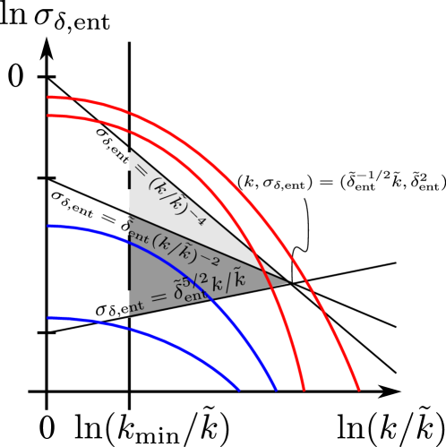
Figure 1: The parameter space of PBH non-formation in the $(k,\sigma_{\delta,\rm ent})$ plane. The shaded regions (Case I: light shaded, Case II: dark shaded) show the parameter region of PBH non-formation. The colored lines represent examples of density perturbation spectra peaked at the PBH scale. From top to bottom, the velocity dispersion does not impede the PBH formation (top red), does do so (bottom red and top blue), and does not do so (bottom blue).

Once the density power spectrum $\sigma^{2}_{\delta,{\rm ent}}(k)$ is given as a function of $k$, and if the line describing the density power spectrum passes across the shaded region in Fig. 1, there exist small-scale perturbations that prevent a density perturbation of an amplitude $\tilde{\delta}_{\rm ent}$ on the scale $\tilde{k}$ to form a PBH. An important point in this diagram is the place where the lines representing the two conditions in (14) and (15) merge. It occurs at $(k,\sigma_{\delta,\rm ent})=(\tilde{\delta}_{\rm ent}^{-1/2}\tilde{k},\tilde{\delta}_{\rm ent}^{2})$.

Let us apply the above result to a couple of simple examples. When we consider the PBH formation, it is often assumed that there is a narrow peak in the power spectrum and abundant PBHs are produced on scales around the peak. In particular, as a comoving wavenumber $k$ and its horizon crossing time $t$ during inflation is related as $k\sim{\mathrm{e}}^{Ht}$, a log-normal distribution is naturally realized in many models of inflation. Then, around the peak of the power spectrum, the power spectrum may be well approximated by a log-normal spectrum:

$$\sigma^{2}_{\delta,{\rm ent}}(k)=\sigma^{2}_{0}\exp\left\{-2\mu\left[\ln\left(\frac{k}{\tilde{k}}\right)\right]^{2}\right\},$$ (16)

or equivalently,

$$\ln\sigma_{\delta,{\rm ent}}(k)=-\mu\left[\ln\left(\frac{k}{\tilde{k}}\right)\right]^{2}+\ln\sigma_{0},$$ (17)

where $\mu$ is the non-dimensional parameter characterizing the width of the log-normal distribution.

First, let us consider the case when $\sigma_{\delta,{\rm ent}}(k_{\rm min})<(k_{\rm min}/\tilde{k})^{-4}$ (blue lines in Fig. 1), namely,

$$\ln\sigma_{0}<\ln\sigma_{\rm cr}(\mu,k_{\rm min})\equiv\mu\left[\ln\left(\frac{k_{\rm min}}{\tilde{k}}\right)\right]^{2}-4\ln\left(\frac{k_{\rm min}}{\tilde{k}}\right).$$ (18)

In this case, since the spectrum must lie below the shaded region in Fig. 1 to form PBHs, we obtain the following inequality as the PBH formation condition (see the first panel in Fig. 2):

$$\ln\left(\frac{k_{\rm min}}{\tilde{k}}\right)+\frac{5}{2}\ln\tilde{\delta}_{\rm ent}>\ln\sigma_{\delta,{\rm ent}}(k_{\rm min})$$ (19)

$$\Leftrightarrow \tilde{\delta}_{\rm ent}>\exp\left[-\frac{2}{5}\mu\left[\ln\left(\frac{k_{\rm min}}{\tilde{k}}\right)\right]^{2}\right]\left(\sigma_{0}\frac{\tilde{k}}{k_{\rm min}}\right)^{2/5}.$$ (20)

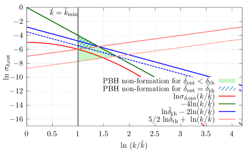
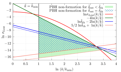
Figure 2: The region for PBH non-formation and the spectral line (red curve) for $\ln\sigma_{0}=-5$ (top panel) and $\ln\sigma_{0}=-2.5$ (bottom panel) with $\ln(k_{\rm min}/\tilde{k})=1$, $\mu=1$ are shown. The top (bottom) panel shows the case for $\sigma_{0}<\sigma_{\rm cr}(\mu,k_{\rm min})$ ($\sigma_{0}>\sigma_{\rm cr}(\mu,k_{\rm min})$), which corresponds to the blue (red) curves in Fig. 1. For $\tilde{\delta}_{\rm ent}<\tilde{\delta}_{\rm th}$ with $\tilde{\delta}_{\rm th}$ being defined in Eq. (24), the lines for $\ln\sigma_{\delta,{\rm ent}}=\ln\tilde{\delta}_{\rm ent}-2\ln(k/\tilde{k})$ and $\ln\sigma_{\delta,{\rm ent}}=5/2\ln\tilde{\delta}_{\rm ent}+\ln(k/\tilde{k})$ are shown by the blue and orange dashed lines, respectively. The green-shaded region is the region for PBH non-formation. Since the spectral line (red curve) passes through the green-shaded region, in this case, there exist small-scale perturbations that prevent the PBH formation on the scale $\tilde{k}$. If $\tilde{\delta}_{\rm ent}$ is increased to the threshold value, i.e., $\tilde{\delta}_{\rm ent}=\tilde{\delta}_{\rm th}$, the blue and orange dashed lines get shifted up to the corresponding solid lines, so that the shaded triangle region of non-formation becomes narrower to the hatched triangle and touches the spectral line at a vertex.

In the case $\sigma_{\delta,{\rm ent}}(k_{\rm min})>(k_{\rm min}/\tilde{k})^{-4}$ (red lines in Fig. 1), namely,

$$\ln\sigma_{0}>\ln\sigma_{\rm cr}(\mu,k_{\rm min}),$$ (21)

the spectrum must lie above the shaded region to form PBHs. This condition is satisfied if the point $(k,\sigma_{\delta,\rm ent})=(\tilde{\delta}_{\rm ent}^{-1/2}\tilde{k},\tilde{\delta}_{\rm ent}^{2})$ is below the spectral curve. This leads to the condition,

$$2\ln\tilde{\delta}_{\rm ent} < \ln\sigma_{\delta,{\rm ent}}\left(k=\tilde{\delta}_{\rm ent}^{-1/2}\tilde{k}\right)=-\mu\left(\ln\tilde{\delta}_{\rm ent}^{-1/2}\right)^{2}+\ln\sigma_{0}\,.$$ (22)

Noting that $\tilde{\delta}_{\rm ent}<1$, we find that the inequality (22) implies the condition (see the second panel in Fig. 2),

$$\tilde{\delta}_{\rm ent}>\exp\left[-\frac{2}{\mu}\left(2+\sqrt{4+\mu\ln\sigma_{0}}\right)\right].$$ (23)

To summarize, the necessary condition for the PBH formation, (20) and (23), is

$$\tilde{\delta}_{\rm ent}>\tilde{\delta}_{\rm th}(\sigma_{0},\mu,k_{\rm min})\equiv\left\{\begin{array}[]{ccl}\exp\left[-\dfrac{2}{5}\mu\ln^{2}\left({k_{\rm min}}/{\tilde{k}}\right)\right]\left(\sigma_{0}({\tilde{k}}/{k_{\rm min}})\right)^{2/5}&;&\sigma_{0}<\sigma_{\rm cr}(\mu,k_{\rm min}),\\ \exp\left[-\dfrac{2}{\mu}\left(2+\sqrt{4+\mu\ln\sigma_{0}}\right)\right]&;&\sigma_{0}>\sigma_{\rm cr}(\mu,k_{\rm min}).\end{array}\right.$$ (24)

We note that, as is explicitly shown in Fig. 3, $\tilde{\delta}_{\rm th}$ is discontinuous at $\sigma_{0}=\sigma_{\rm cr}(\mu,k_{\rm min})$ as a function of $\sigma_{0}$ if

$$\left.\frac{d\ln\sigma_{\delta,{\rm ent}}(k)}{d\ln k}\right|_{k=k_{\rm min}}>-4\quad\Leftrightarrow\quad\mu\ln\left(\frac{k_{\rm min}}{\tilde{k}}\right)<2\,.$$ (25)

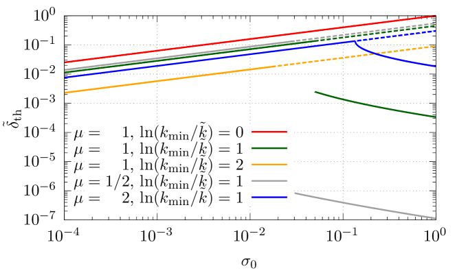
Figure 3: The density threshold $\tilde{\delta}_{\rm th}(\sigma_{0},\mu,k_{\rm min})$ for PBH formation as a function of $\sigma_{0}$ for $(\mu,\ln(k_{\rm min}/\tilde{k}))=(1,0)$, $(1,1)$, $(1,2)$, $(1/2,1)$ and $(2,1)$.

Some comments on the presence of the discontinuity in $\tilde{\delta}_{\rm th}$ are in order. If the root-mean-square value of perturbations on the small scale $\sigma_{\delta,\rm ent}(k)$ is large enough, the resulting virialized halos in a PBH scale region become so compact that they behave like particles at rest and never impede the PBH formation. On the other hand, if $\sigma_{\delta,\rm ent}(k)$ is very small, the velocity dispersion becomes too small to affect the PBH formation. Thus the presence of the discontinuity reflects the fact that the velocity dispersion becomes an effective impeding factor only for a finite range of $\sigma_{\delta,\rm ent}(k)$. This results in the two types of spectra that may lead to the PBH formation, as shown by the top red and the bottom blue curves in Fig. 1. The transition from one type to the other corresponds to the discontinuity. On general grounds, however, one may expect that such a discontinuity would be smoothened when we improve the analyses. For example, we required $\Delta\tilde{t}_{\text{cross}}<\Delta\tilde{t}_{\text{ff}}$ for the non-formation of PBHs, but the fate of would-be PBH over-dense regions may be probabilistic when $\Delta\tilde{t}_{\text{cross}}\simeq\Delta\tilde{t}_{\text{ff}}$. In addition, once we take into account the other impeding factors which we ignored in this paper, namely, asphericity [86], angular momentum [87], and inhomogeneity [82, 83, 88], the discontinuity will not play any role in determining the PBH formation threshold for most of the parameter space of our interest (compare Figs. 3 and 4).

For cosmological applications, one may expect that the width of the peak $\mu$ of the log-normal spectrum (17) would be of order unity, whereas the peak height $\sigma_{0}$ would not be very close to unity since otherwise PBHs would be overproduced. Thus we expect that $\sigma_{0}<\sigma_{\rm cr}$ and the threshold in the first line of Eq. (24), $\tilde{\delta}_{\rm th}\propto\sigma_{0}^{2/5}$, or the condition from Case II, is likely to be relevant in such cases. We mention that if the peak is very sharp so that the width of the spectrum is much less than $k_{\rm min}$, namely, $\mu\ln^{2}(k_{\rm min}/\tilde{k})\gg 1$, the velocity dispersion becomes completely ineffective. In such a case, the other impeding factors we mentioned above will play a decisive role.

5 PBH Formation Probability

In this section, we consider the PBH formation probability by taking into account not only the effect of velocity dispersion but also all the other impeding factors discussed previously in the literature. First, let us recall the effect of angular momentum discussed in Ref. [87]. The threshold values due to the angular momentum estimated at first- and second-order perturbations are given in Eq. (4.12) in Ref. [87] as

$$\tilde{\delta}_{\rm th(1)} = \frac{3\cdot 2^{2}}{5^{3}}q^{2},$$ (26)

$$\tilde{\delta}_{\rm th(2)} = \left(\frac{2}{5}\mathcal{I}\sigma_{0}\right)^{2/3},$$ (27)

where $q$ and $\mathcal{I}$ are parameters of order unity describing the initial reduced quadrupole moment and the second-order tidal contribution to the angular momentum, respectively, and $\sigma_{0}$ is the standard deviation of the density perturbation at the PBH scale. Assuming $q$ is independent of $\sigma_{0}$, the different dependence of the two thresholds on $\sigma_{0}$ leads to different shapes of the PBH production probabilities as shown in Fig. 4.

Second, let us turn to the effect of anisotropy. According to Ref. [86], in an MD era, taking the anisotropy of the system into account, the PBH production probability $\beta_{0}$ is estimated as

$$\beta_{0}\simeq\int_{0}^{\infty}\mathrm{d}\alpha\int_{-\infty}^{\alpha}\mathrm{d}\beta\int_{-\infty}^{\beta}\mathrm{d}\gamma\,\Theta\left(\tilde{\delta}(\alpha,\beta,\gamma)-\delta_{\text{th}}\right)\Theta(1-h(\alpha,\beta,\gamma))w(\alpha,\beta,\gamma),$$ (28)

where $\alpha$, $\beta$, and $\gamma$ are the variables representing the anisotropy, $\Theta(\cdot)$ is the Heaviside step function, $\tilde{\delta}(\alpha,\beta,\gamma)=\alpha+\beta+\gamma$ is the density perturbation in terms of the anisotropy parameters, $h(\alpha,\beta,\gamma)$ is a function that determines the threshold based on the hoop conjecture [92], and $w(\alpha,\beta,\gamma)\propto\exp\left[-3\left(2(\alpha^{2}+\beta^{2}+\gamma^{2})-(\alpha\beta+\beta\gamma+\gamma\alpha)\right)/(2\sigma_{0}^{2})\right]$ is the Doroshkevich probability distribution function [93]. The result is that $\beta_{0}\propto\sigma_{0}^{5}$ with $\tilde{\delta}_{\rm th}=0$. See Refs. [86, 87] for more details.

Finally, let us consider the effect of inhomogeneities discussed in [88]. Their result indicates that $\beta_{0}\propto\sigma^{3/2}$ if only the effect of inhomogeneities is taken into account. If we assume this impeding effect to work independently of the effect of anisotropy, we would obtain $\beta_{0}\propto\sigma^{5}\times\sigma^{3/2}=\sigma^{13/2}$. However, as noted in [88], the threshold obtained there is a sufficient condition for the PBH formation. In other words, it is not a necessary condition for PBH formation. Therefore, to be conservative, we do not take its effect into account in this paper.

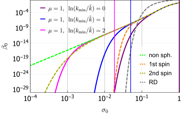
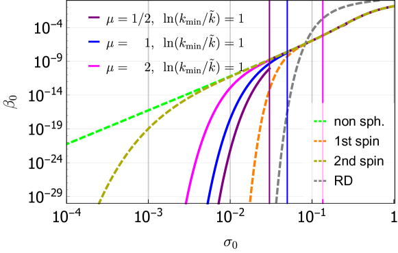
Figure 4: The dependence of the PBH production probability $\beta_{0}$ on the standard deviation $\sigma_{0}$ of the density perturbations at the PBH scale. The solid curves are our results including the effects of velocity dispersion for $(\mu,\ln(k_{\rm min}/\tilde{k}))=(1,0)$ (top panel; purple), $(1,1)$ (both panels; blue), $(1,2)$ (top panel; magenta), $(1/2,1)$ (bottom panel; purple), and $(2,1)$ (bottom panel; magenta). The vertical solid lines indicate the corresponding values of $\sigma_{\rm cr}$. For comparison, the first-order and second-order results in Ref. [87] are plotted as the orange (right) and dark orange (left) dashed lines, respectively. For these, parameters are chosen as $\mathcal{I}=1$ and $q=\sqrt{2}$ [87]. The common slope $\beta_{0}\simeq 0.05556\,\sigma_{0}^{5}$ represented by the green dashed line is the effect of anisotropy [86]. For comparison, the prediction of Carr’s formula $\mathrm{Erfc}[\tilde{\delta}_{\text{th}}/(\sqrt{2}\sigma_{0})]/2$ for the PBH production in the RD era is also shown by the dashed gray line with $\tilde{\delta}_{\text{th}}=0.42$.

In Fig. 4, we plot $\beta_{0}$ with $\tilde{\delta}_{\text{th}}$ determined by the consideration of the velocity dispersion using Eq. (24). For comparison, we also plot $\beta_{0}$ with $\tilde{\delta}_{\text{th}}$ determined by the consideration of the spin effects [87] using Eqs. (26) and (27). The common slope can be approximated as $\beta_{0}\simeq 0.05556\,\sigma_{0}^{5}$ [86] (green dashed line). This is the effect of anisotropy. Different criteria on the density threshold result in different exponential falloffs. They can be understood by Carr’s formula [94], according to which the PBH formation probability is roughly proportional to $\exp[-\tilde{\delta}_{\rm th}^{2}/(2\sigma_{0}^{2})]$. Applying this to our result (24) in the case $\sigma_{0}<\sigma_{\rm cr}$, $\tilde{\delta}_{\rm th}^{2}\propto\sigma_{0}^{4/5}$, the exponent is found to be proportional to $\sigma_{0}^{-6/5}$, as shown by the solid curves in Fig. 4. On the other hand, the exponents are proportional to $\sigma_{0}^{-2}$ and $\sigma_{0}^{-2/3}$, respectively, for the first-order and second-order spin effects, respectively, as shown by the orange dashed (first-order) and dark orange dashed (second-order) curves.

From Fig. 4, we see that the effect of the velocity dispersion can be the dominant factor against the PBH formation. Although the value of $\sigma_{0}$ where the probability exponentially drops significantly depends on $k_{\mathrm{min}}$, if the first-order spin effect is small, which is the case if $q\ll 1$, or if $k_{\mathrm{min}}\simeq\tilde{k}$, the effect of the velocity dispersion is most significant. Here it should be noted that, in reality, all the impeding factors should be taken into account at the same time although we treated the effects of the spin and the velocity dispersion independently in this paper.

6 Conclusions

In this paper, we discussed the effect of velocity dispersion on PBH formation. For this purpose, we considered two distinct scales: One is a large scale that would form a PBH, called the PBH scale, if there were no impeeding factors. The other is a small scale on which the velocity dispersion is generated. Then we derived the condition for the velocity dispersion on the small scale to impede the PBH formation. Once the velocity dispersion is shared in the whole collapsing region, the diffusion associated with the velocity dispersion competes with the gravitational contraction. We obtained the simple criterion $\sigma_{v*}\tilde{R}_{*}<3\tilde{M}$ for the formation of a black hole of mass $\tilde{M}$ in terms of the size $\tilde{R}_{*}$ and the velocity dispersion $\sigma_{v*}$ at the time when the velocity dispersion is shared in the whole region (see Eq. (9)). To apply this formula to the PBH formation, we considered two scenarios of the process.

If the density perturbation on the small scale is sufficiently large, the virialization takes place before the collapsing time of the PBH scale. Then, the velocity dispersion in the virialized halos is released to the whole would-be PBH region when the mean density of that region becomes comparable to the virial density of halos, and it may impede PBH formation. However, if the density perturbation on the small scale is extremely large, the virialized halos become too compact and dense, and the dissolution of halos takes place too late to impede the PBH formation. Thus we obtain an upper bound for the amplitude of the small-scale density perturbation below which the PBH formation is impeded.

On the other hand, if the density perturbation on the small scale is extremely small, the virialization can never be achieved before a PBH is formed. However, even in this case, if the small-scale density perturbation is not too small, it grows and may eventually enter the nonlinear regime. This growth of the small-scale perturbation is enhanced by the fact that it behaves like a perturbation in a closed collapsing background universe which the would-be PBH region mimics. Then assuming that the velocity dispersion is generated and shared over the PBH scale when the amplitude of the small-scale density perturbation exceeds unity, the PBH formation may be impeded. Thus, this scenario renders the perturbation with a somewhat smaller amplitude to impede the PBH formation.

The two conditions are summarized in the inequalities (14) and (15). These conditions can, in principle, apply to any functional form of the density power spectrum. Based on this result, we computed the PBH production rate, assuming that the power spectrum is of a log-normal form, with the peak at the PBH scale. The result is shown in Fig. 4, where comparisons with the other impeding factors, namely anisotropy and angular momentum, are also made. We find that the effect of velocity dispersion can be a dominant factor to prevent PBH formation, although all these effects are subjected to various uncertainties, in addition to the spectral shape dependence, that affects the threshold value of the density perturbation amplitude. It should be also noted that, if the spectrum has a sufficiently sharp peak around the PBH scale, the velocity dispersion is likely to be ineffective. When we translate the observational constraints on the PBH abundance into those on model parameters in PBH formation scenarios, since the effect of the velocity dispersion may act as an additional factor to prevent PBH formation, the allowed regions for the model parameters will get wider (see Figs. 10 and 11 in Ref. [13] for the observational constraints on the PBH abundance).

One of the future directions is to properly include the effect of deviations from the idealized dust picture during the collapse. Besides the apparent fact that the collapsing matter is not dust but collisionless cold particles in the simplest situation, which naturally gives rise to the dispersion in the momentum space as well as in the real space, if it interacts with each other or with other fields non-gravitationally, an additional pressure arises during virialization. If the matter is a massive scalar field, the quantum pressure due to the uncertainty principle may play an essential role. Recently, the PBH formation right after inflation when the inflaton is oscillating, which is effectively an MD era, has been discussed in Refs. [95, 96, 97, 98, 99, 90, 100, 101]. It will be interesting to extend our general relativistic formalisms to these setups.

Appendix A Generation of Velocity Dispersion

A.1 Closed FLRW Collapsing Model

To describe the evolution of over-dense regions, we introduce closed FLRW universes as models for the over-dense regions. We assume that the closed FLRW model can be applied to all over-dense regions on any scale, that is, they can apply to both scales of $\tilde{k}$ and $k$. Therefore, the equations given in this section can be applied to the scale $\tilde{k}$ replacing all the bare quantities ($a_{\rm ent}$, $\Omega_{\rm ent}$, $t_{\rm ent}$, $t_{\rm coll}$, $H_{\rm ent}$, $\delta_{\rm ent}$, $R_{\rm ent}$, $E$, $\mathcal{K}$ and $M$) by the corresponding tilded quantities ($\tilde{a}_{\rm ent}$, $\tilde{\Omega}_{\rm ent}$, $\tilde{t}_{\rm ent}$, $\tilde{t}_{\rm coll}$, $\tilde{H}_{\rm ent}$, $\tilde{\delta}_{\rm ent}$, $\tilde{R}_{\rm ent}$, $\tilde{E}$, $\tilde{\mathcal{K}}$ and $\tilde{M}$).

The Friedmann equation for a closed universe can be written in the following form:

$$\left(\frac{\dot{a}}{a}\right)^{2}= H_{\text{ent}}^{2}\left[\Omega_{\text{ent}}\left(\frac{a_{\text{ent}}}{a}\right)^{3}+\left(1-\Omega_{\text{ent}}\right)\left(\frac{a_{\text{ent}}}{a}\right)^{2}\right],$$ (29)

where $a$, $H_{\rm ent}$ and $\Omega_{\rm ent}$ are the scale factor, Hubble parameter, and cosmological density parameter at the horizon entry $t=t_{\rm ent}=2/(3H_{\text{ent}})$, respectively. Note that, at this stage, the horizon entry time is just the time for reference because we have not introduced the scale of the over-dense region. The spatial curvature $\mathcal{K}$ is given by

$$\mathcal{K}:=(\Omega_{\rm ent}-1)H_{\rm ent}^{2}a_{\rm ent}^{2}.$$ (30)

The parametric solution for the scale factor $a$ is

$$\frac{a}{a_{\text{ent}}}= \frac{\Omega_{\text{ent}}}{2(\Omega_{\text{ent}}-1)}(1-\cos\theta),$$ (31)

$$t= \frac{\Omega_{\text{ent}}}{2H_{\text{ent}}(\Omega_{\text{ent}}-1)^{3/2}}(\theta-\sin\theta),$$ (32)

where the parameter $\theta$ is related to the conformal time $\eta$ by $\theta=\sqrt{\mathcal{K}}\eta$.

Taking the Einstein-de Sitter (EdS) universe as the background universe and considering the uniform Hubble slice, we can obtain the value of the density perturbation at the horizon entry as

$$\delta_{\rm ent}=\Omega_{\rm ent}-1,$$ (33)

where we have used the fact that the background density is given by the critical density $3H^{2}/(8\pi)$ for the uniform Hubble slice. Hereafter we assume $\delta_{\text{ent}}\ll 1$, which can be satisfied even for a rarely high-density region leading to PBH formation in an MD era.

For $\theta=\sqrt{\mathcal{K}}\eta\ll 1$, we find $a\propto t^{2/3}$ at the leading order, and the over-dense region can be approximated by an EdS universe. More specifically, we find

$$\frac{a}{a_{\text{ent}}}= \frac{\Omega_{\rm ent}}{4(\Omega_{\rm ent}-1)}\mathcal{K}\eta^{2}+\frac{1}{\Omega_{\rm ent}-1}\mathcal{O}\left[(\mathcal{K}\eta^{2})^{2}\right],$$ (34)

$$t= \frac{\Omega_{\rm ent}a_{\rm ent}\eta}{12(\Omega_{\rm ent}-1)}\mathcal{K}\eta^{2}+\frac{a_{\rm ent}\eta}{\Omega_{\rm ent}-1}\mathcal{O}\left[(\mathcal{K}\eta^{2})^{2}\right].$$ (35)

Since the value of $\eta$ at the horizon entry is given by $\eta_{\rm ent}\sim 1/(H_{\rm ent}a_{\rm ent})\sim\delta_{\rm ent}/\sqrt{\mathcal{K}}$, we find $\eta<\eta_{\rm ent}\ll 1/\sqrt{\mathcal{K}}$ before the horizon entry, and then the EdS approximation is valid before the horizon entry. The time at the maximum expansion ($\theta=\pi$), $t_{\text{max}}$, and the collapsing time ($\theta=2\pi$), $t_{\text{coll}}$, are given by

$$t_{\text{coll}}=2t_{\rm max}=\frac{\pi\Omega_{\rm ent}}{H_{\text{ent}}(\Omega_{\rm ent}-1)^{3/2}}\simeq \frac{\pi}{H_{\text{ent}}\delta_{\text{ent}}^{3/2}}.$$ (36)

At the maximum expansion, the radius of the over-dense region, $R_{\text{max}}$, becomes

$$R_{\text{max}}\simeq\frac{1}{H_{\text{ent}}\delta_{\text{ent}}}=\frac{R_{\text{ent}}}{\delta_{\text{ent}}}.$$ (37)

At this moment, the energy of the over-dense region can be parametrized as

$$E=-h\frac{M^{2}}{R_{\text{max}}}$$ (38)

with $M=1/(2H_{\text{ent}})$ being the horizon mass at the horizon entry and $h$ is an $\mathcal{O}(1)$ dimensionless parameter. For a uniform ball, $h=3/5$.

A.2 Virialization

After the collapse, if a black hole does not form, the collapsed region is expected to be virialized in a time scale comparable to the collapsing time,

$$t_{\text{vir}}=st_{\text{coll}},$$ (39)

with $s=\mathcal{O}(1)>1$ being another dimensionless parameter. Let us consider the generation process of the velocity dispersion and how it can be shared in the whole region of the scale $\tilde{k}$. As is stated in Sec. 2, here we consider two possible scenarios depending on whether the virialization of the scale $k$ can be realized before $t=\tilde{t}_{\rm coll}$ or not. The condition for the realization of the virialization is given by

$$t_{\rm vir}=st_{\rm coll}<\tilde{t}_{\rm coll}.$$ (40)

By using Eq. (36), the inequality can be rewritten as

$$\qquad sH_{\rm ent}^{-1}\delta_{\rm ent}^{-3/2}<\tilde{H}_{\rm ent}^{-1}\tilde{\delta}_{\rm ent}^{-3/2}$$

$$\Leftrightarrow \qquad sk^{-3}\delta_{\rm ent}^{-3/2}<\tilde{k}^{-3}\tilde{\delta}_{\rm ent}^{-3/2}$$

$$\Leftrightarrow \qquad\frac{k^{2}}{\tilde{k}^{2}}\frac{\delta_{\rm ent}}{\tilde{\delta}_{\rm ent}}>s^{2/3}=\mathcal{O}(1),$$ (41)

where we have used the relation $\tilde{H}_{\rm ent}/H_{\rm ent}=\tilde{k}^{3}/k^{3}$. Hereafter we individually discuss the two cases $t_{\rm vir}<\tilde{t}_{\rm coll}$ (case I) and $t_{\rm vir}>\tilde{t}_{\rm coll}$ (case II) in subsections A.3 and A.4, respectively.

A.3 Case I: Generation through the Virialization

Here, we consider the case $t_{\rm vir}=st_{\rm coll}<\tilde{t}_{\rm coll}$, namely, the condition (41) is satisfied. The virial theorem states that the kinetic energy $K$ and the potential energy $U$ satisfies $K=-U/2=h{M^{2}}/{R_{\rm vir}}$, where $R_{\rm vir}$ is the radius of the virialized halo. Since the total energy is conserved and is given by $-h{M^{2}}/{R_{\rm max}}$ at the maximum expansion, we obtain

$$E=K+U=-K=-\frac{1}{2}M\sigma_{v}^{2}=-h\frac{M^{2}}{R_{\rm max}}.$$ (42)

From this equation, we find

$$\sigma_{v}^{2}=2h\frac{M}{R_{\rm max}}=h\frac{2M}{R_{\rm ent}}\frac{R_{\rm ent}}{R_{\rm max}}\simeq h\delta_{\rm ent},$$ (43)

where we used $2M=R_{\rm ent}$ and Eq. (37). In addition, from $E=U/2=U_{\rm max}$, we find $R_{\rm vir}=R_{\rm max}/2$, or equivalently,

$$\rho_{\rm vir}=8\rho_{\rm max}\simeq 8\rho_{\rm ent}\delta_{\rm ent}^{3}.$$ (44)

The virialized halos behave as macroscopic particles until the mean density of the scale $\tilde{k}$ becomes comparable to the virial density $\rho_{\rm vir}$. Thus, we identify the time $t=t_{*}$ by $\tilde{\rho}(t_{*})=\rho_{\rm vir}=8\rho_{\rm ent}\delta_{\rm ent}^{3}$. This equation can be rewritten as

$$2\delta_{\rm ent}=\left(\frac{\tilde{\rho}(t_{*})}{\rho_{\rm ent}}\right)^{1/3}=\frac{\tilde{R}(t_{\rm ent})}{\tilde{R}(t_{*})}=\frac{\tilde{R}_{\rm ent}}{\tilde{R}(t_{*})}\frac{a_{\rm ent}}{\tilde{a}_{\rm ent}}=\frac{\tilde{R}_{\rm ent}}{\tilde{R}(t_{*})}\frac{\tilde{k}^{2}}{k^{2}}.$$ (45)

From this equation and $\sigma_{v}^{2}(t_{*})\simeq h\delta_{\rm ent}$, we obtain

$$\sigma_{v}^{2}(t_{*})\tilde{R}^{2}(t_{*})\simeq\frac{h}{4\delta_{\rm ent}}\frac{\tilde{k}^{4}}{k^{4}}\tilde{R}_{\rm ent}^{2}.$$ (46)

Then, the condition (9) can be reduced to

$$\delta_{\rm ent}<\frac{h}{9}\frac{\tilde{k}^{4}}{k^{4}}.$$ (47)

At first glance, the last inequality seems counterintuitive because we need a smaller value of $\delta_{\rm ent}$ to obtain the significant effect of the velocity dispersion originating from the smaller scale perturbations. However, this inequality indeed makes sense as follows. Since the virial radius is given by $R_{\rm vir}=R_{\rm ent}/({2\delta_{\rm ent}})$, the larger $\delta_{\rm ent}$ is, the smaller the size of the virialized halos becomes. Therefore, under the condition that the virialization is realized before $t=\tilde{t}_{\rm coll}$, if the value of $\delta_{\rm ent}$ is larger than the critical value, the virialized halos are too small and the halo dissolution is too late to prevent PBH formation.

A.4 Case II: Direct Generation from nonlinear Perturbations

Here we consider the case $t_{\rm vir}=st_{\rm coll}>\tilde{t}_{\rm coll}$, namely, the following inequality is satisfied:

$$\frac{k^{2}}{\tilde{k}^{2}}\frac{\delta_{\rm ent}}{\tilde{\delta}_{\rm ent}}>s^{2/3}=\mathcal{O}(1).$$ (48)

Even in this case, the growth of the smaller-scale perturbations is promoted as the contraction of the scale $\tilde{k}$ proceeds. Then, the smaller-scale perturbations may get into the nonlinear regime and produce caustics, and velocity dispersion is generated before the collapse of the scale $\tilde{k}$. We assume that the velocity dispersion is shared in the whole region of the scale $\tilde{k}$ at the same time $t_{*}$ of its generation. To quantitatively evaluate the value of the velocity dispersion, let us consider the linear-perturbation equation in the background closed universe.

A.4.1 Density perturbations in the closed FLRW universe

In the comoving gauge, the equation for the density perturbations of the scale $\tilde{k}$ in the closed universe is given by (see, e.g., Ref. [102])

$$(1-\cos\theta)\frac{\mathrm{d}^{2}}{\mathrm{d}\theta^{2}}\delta_{\rm co}+\sin\theta\frac{\mathrm{d}}{\mathrm{d}\theta}\delta_{\rm co}-3\delta_{\rm co}=0.$$ (49)

The growing-mode solution is given as follows (see, e.g., Ref. [102]):

$$\delta_{\rm co}=\frac{\delta_{\rm co,max}}{2}\left(\frac{5+\cos\theta}{1-\cos\theta}-\frac{3\theta\sin\theta}{(1-\cos\theta)^{2}}\right)=\delta_{\rm co,max}\left(\frac{\theta^{2}}{20}+\mathcal{O}(\theta^{4})\right),$$ (50)

where $\delta_{\rm co,max}=\delta_{\rm co}(\pi)$.

In order to relate the evolution of the perturbation $\delta_{\rm co}$ to the density perturbation $\delta$ defined in the flat FLRW model with the uniform Hubble slice, we need to clarify the relation between the values of $\delta_{\rm ent}$ and $\delta_{\rm co,max}$. For this purpose, let us consider the value of $\delta_{\rm co}$ at the horizon entry. The horizon entry of the scale $k$ is earlier than that of the scale $\tilde{k}$, so the EdS approximation is valid at the horizon entry time as is discussed in Sec. A.1. Then, we obtain

$$a_{\rm ent}H_{\rm ent}=k,$$ (51)

$$H_{\rm ent}=\tilde{H}_{\rm ent}\frac{k^{3}}{\tilde{k}^{3}}=\frac{2}{3t_{\rm ent}}.$$ (52)

From the second equation, we find

$$t_{\rm ent} = \frac{2}{3\tilde{H}_{\rm ent}}\frac{\tilde{k}^{3}}{k^{3}}.$$ (53)

Let us express $t_{\rm ent}$ by using the conformal time from Eq. (35) as follows:

$$t_{\rm ent}\simeq\frac{1}{12\tilde{H}_{\rm ent}}\left(\tilde{H}_{\rm ent}\tilde{a}_{\rm ent}\eta_{\rm ent}\right)^{3},$$ (54)

where we have used the approximation $\tilde{\Omega}_{\rm ent}\simeq 1$. Then we obtain

$$\eta_{\rm ent}=2\frac{\tilde{k}}{k}\frac{1}{\tilde{a}_{\rm ent}\tilde{H}_{\rm ent}}.$$ (55)

From Eq. (50), we can find

$$\delta_{\rm co,ent}\simeq\tilde{\mathcal{K}}\eta_{\rm ent}^{2}\frac{\delta_{\rm co,max}}{20}=\frac{1}{5}(\tilde{\Omega}_{\rm ent}-1)\frac{\tilde{k}^{2}}{k^{2}}\delta_{\rm co,max}=\frac{1}{5}\frac{\tilde{k}^{2}}{k^{2}}\tilde{\delta}_{\rm ent}\delta_{\rm co,max}.$$ (56)

Rewriting $\delta_{\rm co,max}$ by using $\delta_{\rm co,ent}$, we obtain

$$\delta_{\rm co}=\frac{5}{2}\frac{k^{2}}{\tilde{k}^{2}}\frac{\delta_{\rm co,ent}}{\tilde{\delta}_{\rm ent}}\left(\frac{5+\cos\theta}{1-\cos\theta}-\frac{3\theta\sin\theta}{(1-\cos\theta)^{2}}\right).$$ (57)

It is known that the density perturbations $\delta_{\rm co}$ in the comoving gauge and $\delta$ in the uniform Hubble gauge is related to each other as $\delta_{\rm co}\simeq({3}/{5})\delta$ on super-horizon scales (see, e.g., Ref. [63]). Then, we extrapolate this relation to the horizon entry, that is, we use the relation $\delta_{\rm co,ent}\simeq({3}/{5})\delta_{\rm ent}$. By using this relation, we finally obtain the following expression:

$$\delta_{\rm co}=\frac{3}{2}\frac{k^{2}}{\tilde{k}^{2}}\frac{\delta_{\rm ent}}{\tilde{\delta}_{\rm ent}}\left(\frac{5+\cos\theta}{1-\cos\theta}-\frac{3\theta\sin\theta}{(1-\cos\theta)^{2}}\right).$$ (58)

A.4.2 Estimation of the velocity dispersion

To evaluate the velocity dispersion, we consider the velocity perturbation in the comoving gauge. In the comoving gauge, the velocity potential $\phi_{v}$ is related to the density perturbation as [102]

$$\phi_{v}=-(\triangle+3\tilde{\mathcal{K}})^{-1}\frac{\mathrm{d}}{\mathrm{d}\eta}\delta_{\rm co},$$ (59)

where $\triangle$ is the Laplacian. The spatial curvature contribution can be estimated as $\tilde{\mathcal{K}}=\tilde{\delta}_{\rm ent}\tilde{k}^{2}\ll k^{2}$, and the contribution is negligible compared to the Laplacian term. Then, we have

$$\phi_{v}\simeq k^{-2}\frac{\mathrm{d}}{\mathrm{d}\eta}{\delta}_{\rm co}.$$ (60)

The absolute value $v$ of the velocity can be estimated as follows:

$$v\simeq{k}\phi_{v}\simeq k^{-1}\frac{d}{d\eta}{\delta}_{\rm co}.$$ (61)

From the following equations

$$\tilde{R}(\theta) = \tilde{R}_{\rm ent}\frac{\tilde{a}}{\tilde{a}_{\rm ent}}=\frac{\tilde{R}_{\rm ent}}{2}\frac{\tilde{\Omega}_{\rm ent}}{\tilde{\Omega}_{\rm ent}-1}(1-\cos\theta),$$ (62)

$$v(\theta) \simeq \frac{\frac{\mathrm{d}}{\mathrm{d}\eta}{\delta}_{\rm co}}{k}=\frac{9}{2}\frac{k}{\tilde{k}}\frac{1}{\sqrt{\tilde{\Omega}_{\rm ent}-1}}\delta_{\rm ent}\frac{2\theta+\theta\cos\theta-3\sin\theta}{(1-\cos\theta)^{2}},$$ (63)

we obtain

$$\frac{\tilde{R}(\theta)}{\tilde{R}_{\rm ent}}v(\theta)\simeq\frac{9}{4}\frac{k}{\tilde{k}}\tilde{\delta}_{\rm ent}^{-3/2}\delta_{\rm ent}\frac{2\theta+\theta\cos\theta-3\sin\theta}{1-\cos\theta},$$ (64)

where we have used $\tilde{\Omega}_{\rm ent}-1=\tilde{\delta}_{\rm ent}$.

Let us suppose that the linear perturbations continue to grow until they enter the nonlinear regime, and caustics appear. Assuming this happens around when $\delta_{\rm co}\sim 1$, we adopt the value of $v$ at the time $t=t_{*}$ defined by $\delta_{\rm co}=1$ for the value of $\sigma_{v}(t_{*})$. Letting $\theta_{*}$ denote the value of $\theta$ at $t=t_{*}$, we find

$$1=\delta_{\rm co}(\theta_{*})=\frac{3}{2}\frac{k^{2}}{\tilde{k}^{2}}\frac{\delta_{\rm ent}}{\tilde{\delta}_{\rm ent}}\frac{5-4\cos\theta_{*}-\cos^{2}\theta_{*}-3\theta_{*}\sin\theta_{*}}{(1-\cos\theta_{*})^{2}}.$$ (65)

From the inequality (48), we can find $\theta_{*}\gtrsim 2.2$. Arranging the equation for $\theta_{*}$, we can derive the following equation:

$$(1-\cos\theta_{*})^{-1}=2^{2/3}3^{-2/3}\tilde{\delta}_{\rm ent}^{2/3}\left(\frac{k}{\tilde{k}}\right)^{-4/3}\delta_{\rm ent}^{-2/3}\left(\frac{5-4\cos\theta_{*}-\cos^{2}\theta_{*}-3\theta_{*}\sin\theta_{*}}{\sqrt{1-\cos\theta_{*}}}\right)^{-2/3}.$$ (66)

Substituting this equation into Eq. (64), we obtain

$$\frac{\tilde{R}(\theta_{*})}{\tilde{R}_{\rm ent}}\sigma_{v}(\theta_{*})\simeq\frac{\tilde{R}(\theta_{*})}{\tilde{R}_{\rm ent}}v(\theta_{*})\simeq 3^{4/3}2^{-4/3}\left(\frac{k}{\tilde{k}}\right)^{-1/3}\tilde{\delta}_{\rm ent}^{-5/6}\delta_{\rm ent}^{1/3}\Xi(\theta_{*}),$$ (67)

where

$$\Xi(\theta_{*}):=(2\theta_{*}+\theta_{*}\cos\theta_{*}-3\sin\theta_{*})\left(\frac{5-4\cos\theta_{*}-\cos^{2}\theta_{*}-3\theta_{*}\sin\theta_{*}}{\sqrt{1-\cos\theta_{*}}}\right)^{-2/3}.$$ (68)

Because $\Xi(\theta_{*})$ is a monotonic function of $\theta_{*}$ satisfying $\Xi(2.2)\simeq 0.56$ and $\Xi(2\pi)=(3\pi)^{1/3}\simeq 2.1$, we can treat $\Xi(\theta_{*})$ as a factor of order 1. Then the PBH non-formation condition (9) can be rewritten as

$$b\frac{\tilde{k}}{k}\tilde{\delta}_{\rm ent}^{-5/2}\delta_{\rm ent}>1,$$ (69)

where

$$b:=\frac{3}{2}\Xi^{3}(\theta_{*})=\mathcal{O}(1).$$ (70)

References

- [1] A. M. Ghez et al., “Measuring Distance and Properties of the Milky Way’s Central Supermassive Black Hole with Stellar Orbits,” Astrophys. J. 689 (2008) 1044–1062, arXiv:0808.2870 [astro-ph].
- [2] S. Gillessen, F. Eisenhauer, T. K. Fritz, H. Bartko, K. Dodds-Eden, O. Pfuhl, T. Ott, and R. Genzel, “The orbit of the star S2 around SgrA* from VLT and Keck data,” Astrophys. J. Lett. 707 (2009) L114–L117, arXiv:0910.3069 [astro-ph.GA].
- [3] R. Genzel, F. Eisenhauer, and S. Gillessen, “The Galactic Center Massive Black Hole and Nuclear Star Cluster,” Rev. Mod. Phys. 82 (2010) 3121–3195, arXiv:1006.0064 [astro-ph.GA].
- [4] GRAVITY Collaboration, R. Abuter et al., “Detection of the gravitational redshift in the orbit of the star S2 near the Galactic centre massive black hole,” Astron. Astrophys. 615 (2018) L15, arXiv:1807.09409 [astro-ph.GA].
- [5] LIGO Scientific, Virgo Collaboration, B. P. Abbott et al., “Observation of Gravitational Waves from a Binary Black Hole Merger,” Phys. Rev. Lett. 116 no. 6, (2016) 061102, arXiv:1602.03837 [gr-qc].
- [6] LIGO Scientific, Virgo Collaboration, B. P. Abbott et al., “GWTC-1: A Gravitational-Wave Transient Catalog of Compact Binary Mergers Observed by LIGO and Virgo during the First and Second Observing Runs,” Phys. Rev. X 9 no. 3, (2019) 031040, arXiv:1811.12907 [astro-ph.HE].
- [7] LIGO Scientific, VIRGO Collaboration, R. Abbott et al., “GWTC-2.1: Deep Extended Catalog of Compact Binary Coalescences Observed by LIGO and Virgo During the First Half of the Third Observing Run,” arXiv:2108.01045 [gr-qc].
- [8] Event Horizon Telescope Collaboration, K. Akiyama et al., “First M87 Event Horizon Telescope Results. I. The Shadow of the Supermassive Black Hole,” Astrophys. J. Lett. 875 (2019) L1, arXiv:1906.11238 [astro-ph.GA].
- [9] Y. B. Zel’dovich and I. D. Novikov Astron. Zh. 43 (1966) 758. [Sov. Astron. 10, (1967) 602].
- [10] S. Hawking, “Gravitationally collapsed objects of very low mass,” Mon. Not. Roy. Astron. Soc. 152 (1971) 75.
- [11] B. J. Carr and S. W. Hawking, “Black holes in the early Universe,” Mon. Not. Roy. Astron. Soc. 168 (1974) 399–415.
- [12] B. J. Carr, K. Kohri, Y. Sendouda, and J. Yokoyama, “New cosmological constraints on primordial black holes,” Phys. Rev. D 81 (2010) 104019, arXiv:0912.5297 [astro-ph.CO].
- [13] B. Carr, K. Kohri, Y. Sendouda, and J. Yokoyama, “Constraints on primordial black holes,” Rept. Prog. Phys. 84 no. 11, (2021) 116902, arXiv:2002.12778 [astro-ph.CO].
- [14] B. Carr and F. Kuhnel, “Primordial Black Holes as Dark Matter: Recent Developments,” Ann. Rev. Nucl. Part. Sci. 70 (2020) 355–394, arXiv:2006.02838 [astro-ph.CO].
- [15] A. Escrivà, F. Kuhnel, and Y. Tada, “Primordial Black Holes,” arXiv:2211.05767 [astro-ph.CO].
- [16] S. Bird, I. Cholis, J. B. Muñoz, Y. Ali-Haïmoud, M. Kamionkowski, E. D. Kovetz, A. Raccanelli, and A. G. Riess, “Did LIGO detect dark matter?,” Phys. Rev. Lett. 116 no. 20, (2016) 201301, arXiv:1603.00464 [astro-ph.CO].
- [17] S. Clesse and J. García-Bellido, “The clustering of massive Primordial Black Holes as Dark Matter: measuring their mass distribution with Advanced LIGO,” Phys. Dark Univ. 15 (2017) 142–147, arXiv:1603.05234 [astro-ph.CO].
- [18] M. Sasaki, T. Suyama, T. Tanaka, and S. Yokoyama, “Primordial Black Hole Scenario for the Gravitational-Wave Event GW150914,” Phys. Rev. Lett. 117 no. 6, (2016) 061101, arXiv:1603.08338 [astro-ph.CO]. [Erratum: Phys.Rev.Lett. 121, 059901 (2018)].
- [19] M. Sasaki, T. Suyama, T. Tanaka, and S. Yokoyama, “Primordial black holes—perspectives in gravitational wave astronomy,” Class. Quant. Grav. 35 no. 6, (2018) 063001, arXiv:1801.05235 [astro-ph.CO].
- [20] H. Niikura, M. Takada, S. Yokoyama, T. Sumi, and S. Masaki, “Constraints on Earth-mass primordial black holes from OGLE 5-year microlensing events,” Phys. Rev. D 99 no. 8, (2019) 083503, arXiv:1901.07120 [astro-ph.CO].
- [21] NANOGrav Collaboration, Z. Arzoumanian et al., “The NANOGrav 12.5 yr Data Set: Search for an Isotropic Stochastic Gravitational-wave Background,” Astrophys. J. Lett. 905 no. 2, (2020) L34, arXiv:2009.04496 [astro-ph.HE].
- [22] V. Vaskonen and H. Veermäe, “Did NANOGrav see a signal from primordial black hole formation?,” Phys. Rev. Lett. 126 no. 5, (2021) 051303, arXiv:2009.07832 [astro-ph.CO].
- [23] V. De Luca, G. Franciolini, and A. Riotto, “NANOGrav Data Hints at Primordial Black Holes as Dark Matter,” Phys. Rev. Lett. 126 no. 4, (2021) 041303, arXiv:2009.08268 [astro-ph.CO].
- [24] K. Kohri and T. Terada, “Solar-Mass Primordial Black Holes Explain NANOGrav Hint of Gravitational Waves,” Phys. Lett. B 813 (2021) 136040, arXiv:2009.11853 [astro-ph.CO].
- [25] S. Sugiyama, V. Takhistov, E. Vitagliano, A. Kusenko, M. Sasaki, and M. Takada, “Testing Stochastic Gravitational Wave Signals from Primordial Black Holes with Optical Telescopes,” Phys. Lett. B 814 (2021) 136097, arXiv:2010.02189 [astro-ph.CO].
- [26] G. Domènech and S. Pi, “NANOGrav Hints on Planet-Mass Primordial Black Holes,” arXiv:2010.03976 [astro-ph.CO].
- [27] K. Inomata, M. Kawasaki, K. Mukaida, and T. T. Yanagida, “NANOGrav Results and LIGO-Virgo Primordial Black Holes in Axionlike Curvaton Models,” Phys. Rev. Lett. 126 no. 13, (2021) 131301, arXiv:2011.01270 [astro-ph.CO].
- [28] M. Kawasaki, A. Kusenko, and T. T. Yanagida, “Primordial seeds of supermassive black holes,” Phys. Lett. B 711 (2012) 1–5, arXiv:1202.3848 [astro-ph.CO].
- [29] K. Kohri, T. Nakama, and T. Suyama, “Testing scenarios of primordial black holes being the seeds of supermassive black holes by ultracompact minihalos and CMB -distortions,” Phys. Rev. D 90 no. 8, (2014) 083514, arXiv:1405.5999 [astro-ph.CO].
- [30] T. Nakama, T. Suyama, and J. Yokoyama, “Supermassive black holes formed by direct collapse of inflationary perturbations,” Phys. Rev. D 94 no. 10, (2016) 103522, arXiv:1609.02245 [gr-qc].
- [31] B. Carr and J. Silk, “Primordial Black Holes as Generators of Cosmic Structures,” Mon. Not. Roy. Astron. Soc. 478 no. 3, (2018) 3756–3775, arXiv:1801.00672 [astro-ph.CO].
- [32] P. D. Serpico, V. Poulin, D. Inman, and K. Kohri, “Cosmic microwave background bounds on primordial black holes including dark matter halo accretion,” Phys. Rev. Res. 2 no. 2, (2020) 023204, arXiv:2002.10771 [astro-ph.CO].
- [33] C. Ünal, E. D. Kovetz, and S. P. Patil, “Multimessenger probes of inflationary fluctuations and primordial black holes,” Phys. Rev. D 103 no. 6, (2021) 063519, arXiv:2008.11184 [astro-ph.CO].
- [34] K. Kohri, T. Sekiguchi, and S. Wang, “Cosmological 21-cm line observations to test scenarios of super-Eddington accretion on to black holes being seeds of high-redshifted supermassive black holes,” Phys. Rev. D 106 no. 4, (2022) 043539, arXiv:2201.05300 [astro-ph.CO].
- [35] D. Toussaint, S. B. Treiman, F. Wilczek, and A. Zee, “Matter - Antimatter Accounting, Thermodynamics, and Black Hole Radiation,” Phys. Rev. D 19 (1979) 1036–1045.
- [36] J. D. Barrow, E. J. Copeland, E. W. Kolb, and A. R. Liddle, “Baryogenesis in extended inflation. 2. Baryogenesis via primordial black holes,” Phys. Rev. D 43 (1991) 984–994.
- [37] D. Baumann, P. J. Steinhardt, and N. Turok, “Primordial Black Hole Baryogenesis,” arXiv:hep-th/0703250.
- [38] K. Inomata, M. Kawasaki, K. Mukaida, T. Terada, and T. T. Yanagida, “Gravitational Wave Production right after a Primordial Black Hole Evaporation,” Phys. Rev. D 101 no. 12, (2020) 123533, arXiv:2003.10455 [astro-ph.CO].
- [39] T. Papanikolaou, V. Vennin, and D. Langlois, “Gravitational waves from a universe filled with primordial black holes,” JCAP 03 (2021) 053, arXiv:2010.11573 [astro-ph.CO].
- [40] G. Domènech, C. Lin, and M. Sasaki, “Gravitational wave constraints on the primordial black hole dominated early universe,” JCAP 04 (2021) 062, arXiv:2012.08151 [gr-qc].
- [41] G. Domènech, V. Takhistov, and M. Sasaki, “Exploring Evaporating Primordial Black Holes with Gravitational Waves,” arXiv:2105.06816 [astro-ph.CO].
- [42] N. Bhaumik and R. K. Jain, “Small scale induced gravitational waves from primordial black holes, a stringent lower mass bound, and the imprints of an early matter to radiation transition,” Phys. Rev. D 104 no. 2, (2021) 023531, arXiv:2009.10424 [astro-ph.CO].
- [43] D. Hooper, G. Krnjaic, J. March-Russell, S. D. McDermott, and R. Petrossian-Byrne, “Hot Gravitons and Gravitational Waves From Kerr Black Holes in the Early Universe,” arXiv:2004.00618 [astro-ph.CO].
- [44] K. Inomata, K. Kohri, T. Nakama, and T. Terada, “Enhancement of Gravitational Waves Induced by Scalar Perturbations due to a Sudden Transition from an Early Matter Era to the Radiation Era,” Phys. Rev. D 100 no. 4, (2019) 043532, arXiv:1904.12879 [astro-ph.CO].
- [45] T. Papanikolaou, “Gravitational waves induced from primordial black hole fluctuations: the effect of an extended mass function,” JCAP 10 (2022) 089, arXiv:2207.11041 [astro-ph.CO].
- [46] K. N. Ananda, C. Clarkson, and D. Wands, “The Cosmological gravitational wave background from primordial density perturbations,” Phys. Rev. D 75 (2007) 123518, arXiv:gr-qc/0612013.
- [47] D. Baumann, P. J. Steinhardt, K. Takahashi, and K. Ichiki, “Gravitational Wave Spectrum Induced by Primordial Scalar Perturbations,” Phys. Rev. D 76 (2007) 084019, arXiv:hep-th/0703290.
- [48] R. Saito and J. Yokoyama, “Gravitational wave background as a probe of the primordial black hole abundance,” Phys. Rev. Lett. 102 (2009) 161101, arXiv:0812.4339 [astro-ph]. [Erratum: Phys.Rev.Lett. 107, 069901 (2011)].
- [49] R. Saito and J. Yokoyama, “Gravitational-Wave Constraints on the Abundance of Primordial Black Holes,” Prog. Theor. Phys. 123 (2010) 867–886, arXiv:0912.5317 [astro-ph.CO]. [Erratum: Prog.Theor.Phys. 126, 351–352 (2011)].
- [50] H. Assadullahi and D. Wands, “Gravitational waves from an early matter era,” Phys. Rev. D 79 (2009) 083511, arXiv:0901.0989 [astro-ph.CO].
- [51] J. R. Espinosa, D. Racco, and A. Riotto, “A Cosmological Signature of the SM Higgs Instability: Gravitational Waves,” JCAP 09 (2018) 012, arXiv:1804.07732 [hep-ph].
- [52] K. Kohri and T. Terada, “Semianalytic calculation of gravitational wave spectrum nonlinearly induced from primordial curvature perturbations,” Phys. Rev. D 97 no. 12, (2018) 123532, arXiv:1804.08577 [gr-qc].
- [53] R.-g. Cai, S. Pi, and M. Sasaki, “Gravitational Waves Induced by non-Gaussian Scalar Perturbations,” Phys. Rev. Lett. 122 no. 20, (2019) 201101, arXiv:1810.11000 [astro-ph.CO].
- [54] C. Yuan and Q.-G. Huang, “A topic review on probing primordial black hole dark matter with scalar induced gravitational waves,” arXiv:2103.04739 [astro-ph.GA].
- [55] G. Domènech, “Scalar induced gravitational waves review,” arXiv:2109.01398 [gr-qc].
- [56] M. Shibata and M. Sasaki, “Black hole formation in the Friedmann universe: Formulation and computation in numerical relativity,” Phys. Rev. D 60 (1999) 084002, arXiv:gr-qc/9905064.
- [57] I. Musco, J. C. Miller, and L. Rezzolla, “Computations of primordial black hole formation,” Class. Quant. Grav. 22 (2005) 1405–1424, arXiv:gr-qc/0412063.
- [58] A. G. Polnarev and I. Musco, “Curvature profiles as initial conditions for primordial black hole formation,” Class. Quant. Grav. 24 (2007) 1405–1432, arXiv:gr-qc/0605122.
- [59] I. Musco, J. C. Miller, and A. G. Polnarev, “Primordial black hole formation in the radiative era: Investigation of the critical nature of the collapse,” Class. Quant. Grav. 26 (2009) 235001, arXiv:0811.1452 [gr-qc].
- [60] I. Musco and J. C. Miller, “Primordial black hole formation in the early universe: critical behaviour and self-similarity,” Class. Quant. Grav. 30 (2013) 145009, arXiv:1201.2379 [gr-qc].
- [61] T. Nakama, T. Harada, A. G. Polnarev, and J. Yokoyama, “Identifying the most crucial parameters of the initial curvature profile for primordial black hole formation,” JCAP 01 (2014) 037, arXiv:1310.3007 [gr-qc].
- [62] T. Harada, C.-M. Yoo, and K. Kohri, “Threshold of primordial black hole formation,” Phys. Rev. D 88 no. 8, (2013) 084051, arXiv:1309.4201 [astro-ph.CO]. [Erratum: Phys.Rev.D 89, 029903 (2014)].
- [63] T. Harada, C.-M. Yoo, T. Nakama, and Y. Koga, “Cosmological long-wavelength solutions and primordial black hole formation,” Phys. Rev. D 91 no. 8, (2015) 084057, arXiv:1503.03934 [gr-qc].
- [64] I. Musco, “Threshold for primordial black holes: Dependence on the shape of the cosmological perturbations,” Phys. Rev. D 100 no. 12, (2019) 123524, arXiv:1809.02127 [gr-qc].
- [65] A. Escrivà, C. Germani, and R. K. Sheth, “Universal threshold for primordial black hole formation,” Phys. Rev. D 101 no. 4, (2020) 044022, arXiv:1907.13311 [gr-qc].
- [66] I. Musco, V. De Luca, G. Franciolini, and A. Riotto, “Threshold for primordial black holes. II. A simple analytic prescription,” Phys. Rev. D 103 no. 6, (2021) 063538, arXiv:2011.03014 [astro-ph.CO].
- [67] I. Musco and T. Papanikolaou, “Primordial black hole formation for an anisotropic perfect fluid: Initial conditions and estimation of the threshold,” Phys. Rev. D 106 no. 8, (2022) 083017, arXiv:2110.05982 [gr-qc].
- [68] T. Papanikolaou, “Toward the primordial black hole formation threshold in a time-dependent equation-of-state background,” Phys. Rev. D 105 no. 12, (2022) 124055, arXiv:2205.07748 [gr-qc].
- [69] J. M. Bardeen, J. R. Bond, N. Kaiser, and A. S. Szalay, “The statistics of peaks of Gaussian random fields,” Astrophys. J. 304 (May, 1986) 15–61.
- [70] C.-M. Yoo, T. Harada, J. Garriga, and K. Kohri, “Primordial black hole abundance from random Gaussian curvature perturbations and a local density threshold,” PTEP 2018 no. 12, (2018) 123E01, arXiv:1805.03946 [astro-ph.CO].
- [71] C. Germani and I. Musco, “Abundance of Primordial Black Holes Depends on the Shape of the Inflationary Power Spectrum,” Phys. Rev. Lett. 122 no. 14, (2019) 141302, arXiv:1805.04087 [astro-ph.CO].
- [72] C.-M. Yoo, T. Harada, S. Hirano, and K. Kohri, “Abundance of Primordial Black Holes in Peak Theory for an Arbitrary Power Spectrum,” PTEP 2021 no. 1, (2021) 013E02, arXiv:2008.02425 [astro-ph.CO].
- [73] J. C. Niemeyer and K. Jedamzik, “Near-critical gravitational collapse and the initial mass function of primordial black holes,” Phys. Rev. Lett. 80 (1998) 5481–5484, arXiv:astro-ph/9709072.
- [74] J. Yokoyama, “Cosmological constraints on primordial black holes produced in the near critical gravitational collapse,” Phys. Rev. D 58 (1998) 107502, arXiv:gr-qc/9804041.
- [75] A. M. Green and A. R. Liddle, “Critical collapse and the primordial black hole initial mass function,” Phys. Rev. D 60 (1999) 063509, arXiv:astro-ph/9901268.
- [76] F. Kühnel, C. Rampf, and M. Sandstad, “Effects of Critical Collapse on Primordial Black-Hole Mass Spectra,” Eur. Phys. J. C 76 no. 2, (2016) 93, arXiv:1512.00488 [astro-ph.CO].
- [77] N. Kitajima, Y. Tada, S. Yokoyama, and C.-M. Yoo, “Primordial black holes in peak theory with a non-Gaussian tail,” JCAP 10 (2021) 053, arXiv:2109.00791 [astro-ph.CO].
- [78] V. Atal, J. Cid, A. Escrivà, and J. Garriga, “PBH in single field inflation: the effect of shape dispersion and non-Gaussianities,” JCAP 05 (2020) 022, arXiv:1908.11357 [astro-ph.CO].
- [79] C.-M. Yoo, J.-O. Gong, and S. Yokoyama, “Abundance of primordial black holes with local non-Gaussianity in peak theory,” JCAP 09 (2019) 033, arXiv:1906.06790 [astro-ph.CO].
- [80] V. Atal, J. Garriga, and A. Marcos-Caballero, “Primordial black hole formation with non-Gaussian curvature perturbations,” JCAP 09 (2019) 073, arXiv:1905.13202 [astro-ph.CO].
- [81] A. Escrivà, Y. Tada, S. Yokoyama, and C.-M. Yoo, “Simulation of primordial black holes with large negative non-Gaussianity,” JCAP 05 no. 05, (2022) 012, arXiv:2202.01028 [astro-ph.CO].
- [82] M. Y. Khlopov and A. G. Polnarev, “PRIMORDIAL BLACK HOLES AS A COSMOLOGICAL TEST OF GRAND UNIFICATION,” Phys. Lett. B 97 (1980) 383–387.
- [83] A. G. Polnarev and M. Yu. Khlopov, “COSMOLOGY, PRIMORDIAL BLACK HOLES, AND SUPERMASSIVE PARTICLES,” Sov. Phys. Usp. 28 (1985) 213–232. [Usp. Fiz. Nauk145,369(1985)].
- [84] C. C. Lin, L. Mestel, and F. H. Shu, “The Gravitational Collapse of a Uniform Spheroid.,” Astrophys. J. 142 (Nov., 1965) 1431.
- [85] Y. B. Zel’Dovich, “Reprint of 1970A&A…..5…84Z. Gravitational instability: an approximate theory for large density perturbations.,” Astron. Astrophys. 500 (Mar., 1970) 13–18.
- [86] T. Harada, C.-M. Yoo, K. Kohri, K.-i. Nakao, and S. Jhingan, “Primordial black hole formation in the matter-dominated phase of the Universe,” Astrophys. J. 833 no. 1, (2016) 61, arXiv:1609.01588 [astro-ph.CO].
- [87] T. Harada, C.-M. Yoo, K. Kohri, and K.-I. Nakao, “Spins of primordial black holes formed in the matter-dominated phase of the Universe,” Phys. Rev. D 96 no. 8, (2017) 083517, arXiv:1707.03595 [gr-qc]. [Erratum: Phys.Rev.D 99, 069904 (2019)].
- [88] T. Kokubu, K. Kyutoku, K. Kohri, and T. Harada, “Effect of Inhomogeneity on Primordial Black Hole Formation in the Matter Dominated Era,” Phys. Rev. D 98 no. 12, (2018) 123024, arXiv:1810.03490 [astro-ph.CO].
- [89] E. de Jong, J. C. Aurrekoetxea, and E. A. Lim, “Primordial black hole formation with full numerical relativity,” arXiv:2109.04896 [astro-ph.CO].
- [90] L. E. Padilla, J. C. Hidalgo, and K. A. Malik, “A new mechanism for primordial black hole formation during reheating,” arXiv:2110.14584 [astro-ph.CO].
- [91] C.-M. Yoo, “The basics of primordial black hole formation and abundance estimation,” Galaxies 10 no. 6, (2022) , arXiv:2211.13512 [astro-ph.CO].
- [92] K. Thorne, Nonspherical Gravitational Collapse: a Short Review in: Magic without magic: John Archibald Wheeler: A collection of essays in honor of his sixtieth birthday. Freeman, San Francisco, 1972.
- [93] A. G. Doroshkevich, “Spatial structure of perturbations and origin of galactic rotation in fluctuation theory,” Astrophysics 6 (1970) 320.
- [94] B. J. Carr, “The Primordial black hole mass spectrum,” Astrophys. J. 201 (1975) 1–19.
- [95] E. Cotner, A. Kusenko, and V. Takhistov, “Primordial Black Holes from Inflaton Fragmentation into Oscillons,” Phys. Rev. D 98 no. 8, (2018) 083513, arXiv:1801.03321 [astro-ph.CO].
- [96] K. Kohri and T. Terada, “Primordial Black Hole Dark Matter and LIGO/Virgo Merger Rate from Inflation with Running Spectral Indices: Formation in the Matter- and/or Radiation-Dominated Universe,” Class. Quant. Grav. 35 no. 23, (2018) 235017, arXiv:1802.06785 [astro-ph.CO].
- [97] J. Martin, T. Papanikolaou, and V. Vennin, “Primordial black holes from the preheating instability in single-field inflation,” JCAP 01 (2020) 024, arXiv:1907.04236 [astro-ph.CO].
- [98] J. Martin, T. Papanikolaou, L. Pinol, and V. Vennin, “Metric preheating and radiative decay in single-field inflation,” JCAP 05 (2020) 003, arXiv:2002.01820 [astro-ph.CO].
- [99] P. Auclair and V. Vennin, “Primordial black holes from metric preheating: mass fraction in the excursion-set approach,” JCAP 02 (2021) 038, arXiv:2011.05633 [astro-ph.CO].
- [100] B. Eggemeier, B. Schwabe, J. C. Niemeyer, and R. Easther, “Gravitational Collapse in the Post-Inflationary Universe,” arXiv:2110.15109 [astro-ph.CO].
- [101] J. C. Hidalgo, L. E. Padilla, and G. German, “Production of PBHs from inflaton structure,” arXiv:2208.09462 [astro-ph.CO].
- [102] S. Weinberg, Gravitation and Cosmology: Principles and Applications of the General Theory of Relativity. John Wiley and Sons, New York, 1972.