Soft BPR Loss for Dynamic Hard Negative Sampling in Recommender Systems

Abstract.

In recommender systems, leveraging Graph Neural Networks (GNNs) to formulate the bipartite relation between users and items is a promising way. However, powerful negative sampling methods that is adapted to GNN-based recommenders still requires a lot of efforts. One critical gap is that it is rather tough to distinguish real negatives from massive unobserved items during hard negative sampling. Towards this problem, this paper develops a novel hard negative sampling method for GNN-based recommendation systems by simply reformulating the loss function. We conduct various experiments on three datasets, demonstrating that the method proposed outperforms a set of state-of-the-art benchmarks.

1. Introduction

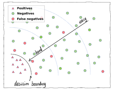
Figure 1. In hard negative sampling of recommender systems, the harder a negative, the more likely it is a false one. It is difficult to distinguish hard negatives and false negatives.

Graph neural network (GNN) based recommender systems have emerged as the most promising way to predict the preferences of users (Wang et al., 2019a; van den Berg et al., 2017; Wang et al., 2019b; He et al., 2020; Huang et al., 2021), in order to avoid information overload in various scenarios, e.g., the personalized recommendations of online music, movies and commodities. Compared to conventional methods in collaborative filtering (CF), such as matrix factorization (Koren, 2008; Salakhutdinov and Mnih, 2007; Koren et al., 2009; Dziugaite and Roy, 2015), recently proposed GNN-based models GCMC (van den Berg et al., 2017), LightGCN (He et al., 2020), and MixGCF (Huang et al., 2021) improve the model prediction accuracy significantly by treating interactions between users and items as a graph, and mining more fine-grained relations among nodes. While most prior efforts focus on GNN-based model structure design (He et al., 2020; van den Berg et al., 2017; Ying et al., 2018; Wang et al., 2019b; Zhang and Chen, 2020; Wang et al., 2019a), another critical component of recommender training, i.e., negative sampling, still has a challenge to achieve effectiveness and efficiency simultaneously (Ding et al., 2020).

Negative sampling is an essential component in implicit CF task. Specifically, in most cases, we can collect users’ implicit feedback, e.g., product purchase or video watching history, and regard these observed user-item interaction pairs as positive targets, since the historical interactions may indicate users’ potential interests. For the remaining large number of unobserved interactions, we need to conduct negative sampling to pick possible negative user-item pairs, trying to avoid false negatives that users may like but have not yet interacted with. Finally, the model is optimized by giving higher rank scores to positive pairs against negatives.

In most previous works, effectiveness is considered as the most critical measurement of the negative sampling strategy in implicit CF task, while another essential criterion, robustness, receives much less attention comparatively. Technically, uniform distribution sampling is commonly adopted in prior efforts (Wang et al., 2019a; He et al., 2020; Huang et al., 2021; Wang et al., 2019b) owing to its efficiency, however, it has been proven less effective due to the lack of capacity to distill high-quality negative samples. To enhance the model effectiveness, there are mainly two negative sampling branches that aim to select hard negatives (i.e. informative negatives) from massive unobserved interaction data, i.e., GAN-based hard samplers (Wang et al., 2017; Park and Chang, 2019; Ding et al., 2019) and dynamic hard samplers (Huang et al., 2021; Ding et al., 2020; Rendle and Freudenthaler, 2014; Huang et al., 2020). GAN-based samplers leverage generative adversarial net (GAN) to iteratively generate hard samples to fool the discriminator, and dynamic hard samplers adaptively select negatives with high matching scores with users. Nevertheless, both kinds of hard negative sampling strategies are less robust, which tend to suffer from severe over-fitting problem in model training. Unfortunately, what underlines such behavior still remains a mystery, thus it rises the question: What is the reason behind the over-fitting?

Contributions

In this paper, we give an answer to the above two questions. First, we investigate why over-fitting problem occurs at the late stage of training process in the hard negative sampling strategy, by controlling the hardness level of negative samples and examining the severity of the over-fitting, respectively. We find empirically that increasing the hardness level will exacerbate model’s over-fitting. To explain it, we introduce the false negative samples, which are users’ potential favorites but are falsely selected as negative samples by the negative sampler. Ding et al. (2020) suggests that a negative with higher hardness level is more likely to be a false negative, therefore, in this paper, we provide a rational explanation that the reason why over-fitting problem generally exists in hard negative samplers is due to the incorrect selection of false negatives. Then, we ask, Is there any possible solution to avoid false negative samples?

This work answers this question by presenting a hard negative sampling strategy, SDNS, that avoids false negatives in an implicit way. The basic idea comes from positive mixing technique (Kalantidis et al., 2020) in contrastive learning, which synthesizes hard negative samples by injecting some information from positive samples, where the positive information just accounts for a small proportion in order to make sure the synthetic negatives mainly made of negative information. However, there is a lack of theoretical analysis on why positive mixing technique works, and ensuring the dominance of negative information in synthetic negatives is just a conservative strategy. To tackle this, we further investigate the impact of positive information on negative synthesizing performance. Unexpectedly, we find empirically that it yields much better experimental results when the synthetic hard negatives are dominated by positive information rather than negative information. Such a counter-intuitive phenomenon motivates us to propose a novel hard negative sampling strategy, Positive-Dominate Negative Synthesizing (SDNS), for implicit CF task. Comprehensive experiments demonstrate that SDNS not only largely mitigates the over-fitting issue, but also obtains a significant performance gain in effectiveness. Meanwhile, we offer theoretical analysis on the mechanism of SDNS, suggesting that SDNS has a great capacity to resist assigning very large gradient magnitudes to the hardest ones among all selected hard negative samples. This behavior implicitly reduces the risk of automatically raising samples’ hardness level when optimizing the loss function, thus is able to avoid selecting massive false negative samples. Based on above analysis, we present a strikingly simple equivalent algorithm of SDNS, where solely the loss objective is slightly modified with a soft factor. SDNS, as an efficient and effective negative sampling strategy, greatly empowers the promising GNN-based recommendation models.

To summarize, the contributions of our work are as follows:

• We conduct study on the over-fitting problem that generally exists in hard negative sampling approaches of implicit CF task, revealing that the presence of false negative samples is the leading cause of over-fitting.

• We propose a striking simple and effective hard negative sampling approach, SDNS, which suits various GNN-based recommendation models, and has a strong capability to mitigate the over-fitting.

• We theoretically study the mechanism of SDNS, disclosing that SDNS can implicitly reduce the risk of selecting false negative samples when optimizing the loss function.

• We demonstrate the superiorities of SDNS over a set of state-of-the-art negative sampling approaches in terms of both robustness and effectiveness, by experimenting on three real-world datasets.

2. Preliminaries and problem

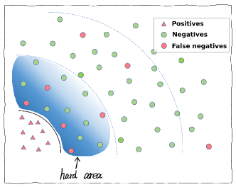
(a) Weighted samples in DNS

(b) Weighted samples in SDNS

Figure 2. The hard area (blue area) covers hard negatives sampled via DNS. Figure (a): without positive-dominated mixing, optimizing BPR loss on these hard negatives will automatically weight the hardest samples too much. Figure (b): with positive-dominated mixing, all hard negatives are given similar weights.

In this section, we formulate the recommendation task as a Bayesian personalized ranking (BPR) problem as common, and then give an overview of hard negative sampling approaches, which play a critical role in recommender training and predicting. Finally, as one of contributions, we find empirically that over-fitting problem exists generally in most hard mining cases.

2.1. Formulation

We define $\mathcal{S}={(u,i)}$ as the training set, containing all observed interactions between each user $u\in\mathcal{U}$ and each item $i\in\mathcal{I}$, (i.e. positive user-item pair $(u,i)$). Note that such positive user-item pairs indicate user $u$ may have a preference on item $i$. The goal of recommendation is to predict users’ preferences and generate a ranked list of items for each user $u$ for personalized recommendation. To achieve this, the common strategy is to sample a number of unobserved pairs $\left\{(u,j)\mid j\notin\mathcal{S}_{u}\right\}$ as negative samples, where $\mathcal{S}_{u}$ is the set of items that have interactions with user $u$. We assume user $u$ dislikes these selected negative samples. Then, the GNN-based recommendation model (such as $LightGCN$ (He et al., 2020) or $NGCF$ (Wang et al., 2019b)) is optimized by giving higher score towards $(u,i)$ than $(u,j)$. Based on this assumption, the widely-adopted loss objective in recommender systems, BPR loss (Rendle et al., 2009), is design as follows:

(1) $$\mathcal{L}_{\mathrm{BPR}}=\sum_{\begin{subarray}{c}(u,i)\in\mathcal{S}\\ j\sim f_{\mathrm{neg}}\end{subarray}}\ln\sigma\left(\hat{y}_{ui}-\hat{y}_{uj}\right),\\$$

(2) $$\text{ with }\ \hat{y}_{ui}=\mathbf{e}_{u}\cdot\mathbf{e}_{i},\textbf{ }\hat{y}_{uj}=\mathbf{e}_{u}\cdot\mathbf{e}_{j},$$

Where $\mathbf{e}_{*}$ is the embedding of $*$ generated by the GNN-based recommendation model, and we apply dot product function to calculate the user-item pair scores. Here, $f_{\mathrm{neg}}$ is the negative sampling function, by which we select the negative sample $j$, and $\sigma(\cdot)$ is a sigmoid function.

In this paper, we derive user and item embeddings by mainly leveraging a state-of-the-art GNN-based model, $LightGCN$, due to its excellent performance over other baselines. The aim of this work is to propose a negative sampling method $f_{\mathrm{neg}}$ that satisfies efficiency and effectiveness simultaneously.

2.2. Hard negative sampling and over-fitting problem

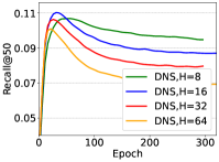
(a) Over-fitting, Taobao

(b) Over-fitting, Tmall

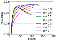
(c) Positive mixing, Taobao

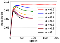
(d) Positive mixing, Tmall

Figure 3. (a)-(b) Over-fitting problem of DNS on two datasets. (c)-(d) Effect of positive mixing in DNS.

As mentioned in Section 1, uniform sampling has been commonly deployed in recommender systems by regarding all unobserved items $\left\{j|j\notin S_{u}\right\}$ having the same probability to be the negative (Wang et al., 2019a; He et al., 2020; Huang et al., 2021; Wang et al., 2019b). But in order to improve the quality of samples, many prior efforts work on picking more informative negatives(a.k.a. hard negatives), by preferring those unobserved items with relatively high matching scores with the user. In doing this, we believe that the model will be challenged and be forced to conduct fine-grained learning. However, over-fitting issue is reported in most works towards hard negative sampling (Huang et al., 2021; Wang et al., 2017; Rendle and Freudenthaler, 2014; Park and Chang, 2019), as in Figure 3(a) and 3(b), the recommender performance drops sharply in the late phase of training process.

To further explore what affects the over-fitting in hard negative sampling of recommender systems, we adopt a straightforward dynamic hard negative sampling strategy, named DNS. Specifically, given a positive user-item pair $(u,i)$, we first form the negative candidate pool $\mathcal{C}$ of size $H$ by uniformly sampling items from non-interacted pairs $\left\{j|j\notin\mathcal{S}_{u}\right\}$, denoted by $\mathcal{C}=\left\{j_{1},j_{2}\dots,j_{H}\right\}$. Then, the hardest negative is selected as:

(3) $$j=\mathop{\arg\max}_{k\in\mathcal{C}}\mathbf{e}_{u}\cdot\mathbf{e}_{k},$$

where $\mathbf{e}_{u}$ and $\mathbf{e}_{k}$ are the embeddings of user $u$ and item $k$, respectively, obtained through a GNN-based recommendation model, e.g., $LightGCN$.

Note that when $H$ is larger, it is easier to select the hard negative samples. Conversely, when $H=1$, it degenerates to the uniform sampling. Thus, the size $H$ of candidate pool $C$ can be used to denote the hardness level of negatives selected (the larger the $H$, the harder the negatives selected). We conduct experiments on two real-world datasets Taobao and Tmall (in Table 1) with $H$ varying in $\left\{8,16,32,64\right\}$, and draw multiple training curves accordingly as Figure 3(a)-3(b). Some observations are as follows:

• Over-fitting problem exists in all four training curves with different negative hardness setting $H$. The performances of DNS soars in the beginning, then degrade dramatically soon after.

• The harder the selected negatives, the severer the over-fitting. For example, the training curve with $H=64$ decreases faster than the one with $H=8$.

• The best performance is achieved when $H=16$ (the peak point, early-stopping strategy is adopted to obtain best model parameters). It is not the case that the recommender performs better along with the increase of the hardness $H$.

Here, we provide an explanation to above three observations, that is, the hard negative sampling strategy is not robust to false negative samples. False negatives are those items that uses may like (potential positive samples), yet are selected as negatives. As in Figure 1, positive samples only account for a small proportion of total items due to the limited historical interactions of users, and false negatives are commonly exist among the rest of items. A critical characteristic of false negatives is that they tend to be assigned high scores by the recommendation model, which makes it difficult to distinguish false negatives and hard negatives. Moreover, the harder the negative, the more likely it is a false one (Ding et al., 2020). (As shown in Figure 1, false negatives are distributed more densely near the decision boundary.) False negatives will provide misleading information to the model optimization, and thus lead to performance degradation. Therefore, we illustrate above observations as follows:

• At the beginning of training process, the recommender is weak in predicting users’ preferences, thus the hard negative selection through DNS tend to be a relatively random selection. The negatives selected are not so hard, and there is little chance to encounter false negatives. So, the recommender performance is improved quickly at first. However, when the recommender becomes more and more accurate, the negatives selected get harder (they get closer to the decision boundary in Figure 1). It is more likely to run into false negatives, leading to a rapid decline of performance.

• The reason of the last two observations is that, when $H$ increases, the hardness level of negatives selected rises. On the one hand, the recommendation training will benefit from real harder negatives (more informative negative samples). On the other hand, high hardness level means the larger possibility of negatives selected falling into false negatives. And including more false negatives in training process will confuse the recommender, degrading model’s performance dramatically (resulting in severer over-fitting). Taking these two aspects into concerns, best performance (the peak point) is achieved when $H=16$.

3. method: Positive-dominated negative synthesizing

In Section 3, we point out the over-fitting problem widely existing in hard negative samplers, and explain it with the presence of false negatives. In this section, firstly, we study the influence of positive mixing technique on recommender training process, which inspires us to propose a positive-dominated negative synthesizing method (SDNS) to generate hard negatives. Next, we offer a theoretical analysis on the loss function and provide a rather simple equivalent algorithm of SDNS. Finally, we conduct extensive experiments on three datasets to demonstrate the superiorities of our method.

3.1. Positive mixing study

In the field of computer vision (CV), developed from $mixup$ (Zhang et al., 2018), positive mixing is a technique to generate synthetic harder negatives from existing negative samples by injecting positive information (Kalantidis et al., 2020). Specifically, for user $u$, positive item $i\in\mathcal{S}_{u}$ and negative item $j\notin\mathcal{S}_{u}$, the synthetic negative instance $\mathbf{e}_{j^{’}}$ from positive mixing can be formulated as follows:

(4) $$\mathbf{e}_{j^{’}}=\alpha\mathbf{e}_{i}+(1-\alpha)\mathbf{e}_{j},\alpha\in P(\cdot)$$

where $\alpha$ is the mixing coefficient that can be drawn from pre-defined distributions $P(\cdot)$, $\mathbf{e}_{i}$ and $\mathbf{e}_{j}$ are embeddings of items $i$ and $j$ respectively, obtained through the recommender $LightGCN$ layers.

In recent works (Kalantidis et al., 2020; Huang et al., 2021), positive mixing strategy is coupled with other techniques, e.g., hardest mixing (Kalantidis et al., 2020) and hop mixing (Huang et al., 2021) to achieve state-of-the-art performances. They claim that positive mixing works as it can generate harder ones compared to original negatives. However, there is a lack of theoretical analysis on it.

In this paper, we investigate how the mixing coefficient $\alpha$ affects the recommender performance. Given item $j$ that is chosen by DNS as a hard negative for user $u$, the synthetic negative embedding from positive mixing $\mathbf{e}_{j^{’}}$ is derived by (4). In MixGCF (Huang et al., 2021), they claim that setting $P(\cdot)$ as uniform distribution $\mathbf{U}(0,1)$ gains advantages over other distributions like Beta distribution and Gaussian distribution. To further explore the influence of the mixing coefficient $\alpha$, here, we just set $\alpha$ as a fixed number $(0\leq\alpha<1)$. Note that when $\alpha=0$, there is no positive information injected, thus it degenerates to basic DNS. As shown in Figure 3(c)-3(d), We observe that:

• In terms of effectiveness, it achieves better performance with large $\alpha$, and yields the best result when $\alpha=0.9$, which outperforms DNS (i.e. $\alpha=0$) by a large margin.

• In terms of robustness, adopting positive mixing with large $\alpha$ can significantly mitigate over-fitting problem.

These two findings are critical, which can be leveraged to enhance the model performance considerably, which are neglected by prior efforts which pay much attention on multi-technique combinations.

3.2. Positive-dominated negative synthesizing (SDNS)

Motivated by above findings, in order to enhance robustness and effectiveness of the recommender, we propose a novel hard negative sampling strategy, i.e., positive-dominated negative synthesizing (SDNS). As an advanced version of DNS, SDNS is easy to implement but efficient, which consists of two steps, i.e., basic DNS selection and positive-dominated mixing.

3.2.1. Conventional DNS

Details are described in Section 2.2.

3.2.2. Positive-dominated mixing

With the observed positive item $i$ and selected hard negative $j$, we synthesize a new hard instance $\mathbf{e}_{j^{’}}$ by injecting a large proportion of positive embedding $\mathbf{e}_{i}$ into $\mathbf{e}_{j}$, formulated as follows:

(5) $$\mathbf{e}_{j}’=\alpha\mathbf{e}_{i}+(1-\alpha)\mathbf{e}_{j}$$

where $\alpha$ is a constant coefficient set normally larger than $0.7$ to ensure the domination of positive information.

3.2.3. Loss function analysis

To further investigate the mechanism of SDNS, we take a closer look at the gradients of two loss objectives w.r.t. DNS and SDNS, separately. Note that in the following functions, leveraging DNS and SDNS as the negative sampling strategy is termed $f_{\mathrm{DNS}}$ and $f_{\mathrm{SDNS}}$ respectively.

BPR loss w.r.t. DNS:

(6) $$\mathcal{L}_{\mathrm{DNS}} =\sum_{\begin{subarray}{c}(u,i)\in\mathcal{S}\\ j\sim f_{\mathrm{DNS}}\end{subarray}}\ln\sigma\left(\mathbf{e}_{u}\cdot\mathbf{e}_{j}-\mathbf{e}_{u}\cdot\mathbf{e}_{i}\right)$$

$$\triangleq\sum_{\begin{subarray}{c}(u,i)\in\mathcal{S}\\ j\sim f_{\mathrm{DNS}}\end{subarray}}\ln\sigma\left(\hat{y}_{uj}-\hat{y}_{ui}\right).$$

Comparatively, BPR loss with SDNS (details are in Appendix):

(7) $$\mathcal{L}_{\mathrm{SDNS}} =\sum_{\begin{subarray}{c}(u,i)\in\mathcal{S}\\ j^{\prime}\sim f_{\mathrm{SDNS}}\end{subarray}}\ln\sigma\left(\mathbf{e}_{u}\cdot\mathbf{e}_{j^{\prime}}-\mathbf{e}_{u}\cdot\mathbf{e}_{i}\right)$$

$$=\sum_{\begin{subarray}{c}(u,i)\in\mathcal{S}\\ j\sim f_{\mathrm{DNS}}\end{subarray}}\ln\sigma\left((1-\alpha)(\hat{y}_{uj}-\hat{y}_{ui})\right).$$

The gradient of $\mathcal{L}_{\mathrm{DNS}}$ w.r.t parameter $\theta\in\Theta$ of the recommendation model, such as $LighGCN$, is as follows:

(8) $$\frac{\partial\mathcal{L}_{\mathbf{DNS}}}{\partial\theta}=\sum_{\begin{subarray}{c}(u,i)\in\mathcal{S}\\ j\sim f_{\mathrm{DNS}}\end{subarray}}\left(1-\sigma\left(\hat{y}_{ui}-\hat{y}_{uj}\right)\right)\frac{\partial\left(\hat{y}_{ui}-\hat{y}_{uj}\right)}{\partial\theta},$$

where for each triplet $(u,i,j)$, we denote its multiplicative scalar $1-\sigma\left(\hat{y}_{ui}-\hat{y}_{uj}\right)$ as $\Delta_{(u,i,j)}^{\mathbf{DNS}}$. It reflects how much the recommendation model learns from the triplet $(u,i,j)$.

Comparatively, the gradient of $\mathcal{L}_{\mathbf{SDNS}}$ is:

(9) $$\frac{\partial\mathcal{L}_{\mathbf{SDNS}}}{\partial\theta}=(1-\alpha)\sum_{\begin{subarray}{c}(u,i)\in\mathcal{S}\\ j\sim f_{\mathrm{DNS}}\end{subarray}}\left(1-\sigma\left((1-\alpha)\left(\hat{y}_{ui}-\hat{y}_{uj}\right)\right)\right)\frac{\partial\left(\hat{y}_{ui}-\hat{y}_{uj}\right)}{\partial\theta},$$

similarly, $1-\sigma\left((1-\alpha)\left(\hat{y}_{ui}-\hat{y}_{uj}\right)\right)$ is defined as $\Delta_{(u,i,j)}^{\mathrm{SDNS}}$.

Note in (9), the first constant coefficient term $(1-\alpha)$ has no influence on model training with optimizer Adam. Thus, the only difference between gradients of $\mathcal{L}_{\mathrm{SDNS}}$ and $\mathcal{L}_{\mathrm{DNS}}$ is that the sigmoid function $\sigma(\cdot)$ is stretched flatter via multiplying by a small number $1-\alpha$, indicating that only stretching $\sigma(\cdot)$ in BPR loss can significantly improve the recommender performance regarding robustness and effectiveness.

To be specific, in DNS, the $\Delta_{(u,i,j)}^{\mathrm{DNS}}$ of different triplets $(u,i,j)$ can be rather different, some of which are near 0 when $\hat{y}_{ui}$ is correctly scored higher than $\hat{y}_{uj}$, while some of which are near 1 when the opposite happens. In the case that $\Delta_{(u,i,j)}^{\mathrm{DNS}}\approx 0$, the recommender learns almost nothing from $(u,i,j)$ pairs, leading to the waste of some hard negatives selected by DNS, and forcing the model to focus on the remaining harder ones. (As shown in Figure 2(a), the hardest samples are weighted too much.) That is, on the one hand, this behavior of BPR loss makes the parameter update based on negatives which are much harder than expectation, thus it is more likely to encounter false negatives and suffer from severe over-fitting. On the other hand, the pairs $(u,i,j)$ with $\Delta_{(u,i,j)}^{\mathrm{DNS}}\approx 0$ are useless in training process, that makes the model less effective due to the loss information.

Comparatively, in SDNS, $\sigma(\cdot)$ is stretched to be flatter, thus the differences among different $\Delta_{(u,i,j)}^{\mathrm{SDNS}}$s are reduced. (As shown in Figure 2(b), all hard negatives are weighted without too much difference.) The effectiveness of the recommendation model is enhanced, since more hard negatives selected from DNS can be involved in training process. Meantime, the algorithm is more robust, because involving more hard negatives means reducing the probability of incorrectly picking false negatives that are densely distributed near decision boundary.

3.3. Equivalent algorithm of SDNS

Input : Training set $\mathcal{S}=\left\{(u,i)\right\}$, recommendation model such as $LightGCN$ with learnable parameter $\Theta$, the size of negative candidate pool $H$.

for $t=1,2,\cdots,T$ do

       Sample a mini-batch $\mathcal{S}_{batch}\in\mathcal{S}$; Initialize loss $\mathcal{L}_{\mathrm{BPR}}^{\mathrm{soft}}$;

       for each $\left(u,i\right)\in\mathcal{S}_{batch}$ do

             Get the embeddings of users and items through the recommendation model;

            Form the negative candidate pool $\mathcal{C}$ by uniformly sample $H$ items from $\left\{j\mid j\notin\mathcal{S}_{u}\right\}$;

            Get the hardest negative item $j$ from $\mathcal{C}$;

            Update $\mathcal{L}_{\mathrm{BPR}}^{\mathrm{soft}}$ (10).

       end for

      Update $\theta$ according to gradient w.r.t. $\mathcal{L}_{\mathrm{BPR}}^{\mathrm{soft}}$ (10).

end for

Algorithm 1 Equivalent algorithm of SDNS

Now, we present an equivalent algorithm by simply modifying BPR loss to suit DNS strategy. By comparing $\mathcal{L}_{\mathrm{DNS}}$ (6) and $\mathcal{L}_{\mathrm{SDNS}}$ (7), it is obvious that applying positive-dominated mixing has the same effect as scaling the sigmoid function in $\mathcal{L}_{\mathrm{DNS}}$. Therefore, we propose a modified BPR loss for DNS as follows:

(10) $$\mathcal{L}_{\mathrm{BPR}}^{\mathrm{soft}}=\sum_{\begin{subarray}{c}(u,i)\in\mathcal{S}\\ j\sim f_{\mathrm{neg}}\end{subarray}}\ln\sigma\left(\left(1-\alpha\right)\left(\hat{y}_{ui}-\hat{y}_{uj}\right)\right).$$

Here, the loss function $\mathcal{L}_{\mathrm{BPR}}^{\mathrm{soft}}$ is soft BPR loss, where $1-\alpha$ is the soft factor, normally set smaller than 0.3 for better performance.

Thus, we develop SDNS into DNS equipped with soft BPR loss, as shown in Algorithm 1, which is not only easy-implemented, solely adding soft factor to BPR loss while maintaining DNS structure unchanged, but also improves performance significantly regarding effectiveness and robustness. In Section 4, Algorithm 1 is utilized for extensive experiments and analysis.

Complexity analysis

As in Algorigm 1, SDNS has the same time complexity and model complexity with conventional DNS, demonstrating one aspect of superiorities over other relatively complicated hard negative mining techniques, especially the time-consuming GAN-based samplers. The selection scheme we present has $O(HT)$ time complexity, where $H$ is the size of negative candidate pool, $T$ denotes the time cost of each score computation. The model complexity of SDNS is $O((|\mathcal{U}|+|\mathcal{I}|)F)$, where $F$ represents the embedding dimension of users and items.

4. EXPERIMENTS

We first conduct experiments on three real-world datasets and compare the performance with various state-of-the-art negative sampling approaches in implicit CF. Then, we conduct hardness study, and replace $LightGCN$ with $NGCF$ as the recommender to verify its generalization ability to other GNN-based models.

4.1. Experimental settings

Table 1. Details of datasets.

Dataset	User	Item	Interaction	Density
Taobao	22,976	29,149	$439,305$	$0.00066$
Tmall	10,000	14,965	$461,899$	$0.00309$
Gowalla	29,858	40,981	$1,027,370$	$0.00084$

Table 2. Performance comparison with LightGCN as the recommender. The last row is relative improvements compared to the strongest baseline (underlined).

	Taobao		Tmall		Gowalla
Method	Recall	NDCG	Recall	NDCG	Recall	NDCG
Uniform	$0.1041$	$0.0378$	$0.0895$	$0.0476$	$0.2712$	$0.1804$
IRGAN	$0.1049$	$0.0380$	$0.0904$	$0.0480$	$0.2799$	$0.1812$
AdvIR	$0.1052$	$0.0382$	$0.0917$	$0.0487$	$0.2710$	$0.1801$
DNS	$0.1107$	$\underline{0.0410}$	$0.0951$	$0.0504$	$\underline{0.2848}$	$\underline{0.1878}$
MixGCF	$\underline{0.1110}$	$0.0403$	$\underline{0.0963}$	$\underline{0.0508}$	$0.2840$	$0.1872$
SDNS	$\mathbf{0.1162}$	$\mathbf{0.0425}$	$\mathbf{0.1051}$	$\mathbf{0.0552}$	$\mathbf{0.2879}$	$\mathbf{0.1906}$
(Proposed)	$4.68\%$	$3.66\%$	$9.14\%$	$8.66\%$	$1.09\%$	$1.49\%$

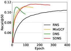
(a) Taobao, LightGCN

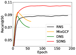
(b) Tmall, LightGCN

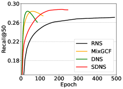
(c) Gowalla, LightGCN

Figure 4. SDNS, DNS, MixGCF, and RNS comparison on three datasets with LightGCN as the recommender.

Datasets

Three real-world datasets, i.e., Taobao, Tmall and Gowalla, are utilized in experiments to evaluate the performance of our method, among which Taobao and Tmall are collected from e-commerce platforms, Gowalla is related to social network. All three datasets contain historical interactions among users and items only. Details are summarized in Table 1.

• Taobao is derived from the e-commerce platform taobao.com, containing various user behaviors, e.g., click, add to cart and buy. To mitigate data sparsity, we regard these different interaction behaviors as positive labels for prediction task. For dataset quality, we randomly choose a subset of users from those with at least 10 interaction records, a.k.a. 10-core setting.

• Tmall is collected from another e-commerce platform tmall. This dataset covers the special period of a large sale event, thus the trading volume is relatively larger than normal. Similarly, we treat multiple behaviors as positive and adopt 10-core setting for customer filtering.

• Gowalla is used for recommendation tasks in social network (Liang et al., 2016; Wang et al., 2019b), consisting of check-in records with users’ locations. We directly utilize the pre-processed dataset in Wang et al. (2019b) for our recommender evaluation.

For each dataset, we sort historical interactions w.r.t. timestamps, then retain the latest $10\%$ records of each user for test set. The rest of interactions are divided by 80/10 to obtain the training set and validation set. Hyper-parameters are tuned according to model’s performance on validation set, and final results on test sets are reported.

Evaluation metrics

A rank list $R_{u}$ consisting of top $N$ items with highest socres will be provided to user $u$ for personalized recommendations. Recall@N and NDCG@N are leveraged as evaluation metrics as in most works, both of which assess the model’s capacity to find potentially relevant items, while NDCG@N accounts more for the position of relevant items in $R_{u}$. $N=50$ is set by default for the following experiments.

Parameter setting

To achieve better performance, we mainly leverage LightGCN (He et al., 2020) as the underlying recommender, but also conduct experiments on NGCF (Wang et al., 2019b) to verify the general effectiveness of the proposed SDNS on GNN-based approaches. For all experiments, the optimizer is Adam and batch size is set as 2048. As for recommenders, we fix their embedding dimension as 64 and the number of aggregation layers in $LightGCN$ or $NGCF$ as 3 by default. Candidate pool size $H$ of DNS, SDNS, and MixGCF is searched in $\left\{8,16,32,64\right\}$ and positive coefficient $\tau$ is tuned in $\left\{0.05,0.1,0.2,0.3,0.4\right\}$. Besides, we search learning rate $l_{r}$ and regularization term $\lambda$ in $\left\{5,10,50,100\right\}*10^{-4}$ and $\left\{0,1,10,100\right\}*10^{-4}$ respectively. For fair comparison with baselines, we report experimental results under their optimal hyper-parameters tuned on validation set.

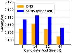
(a) Taobao, LightGCN

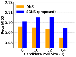
(b) Tmall, LightGCN

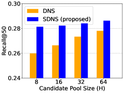
(c) Gowalla, LightGCN

Figure 5. Impact of the size of negative candidate pool ($H$)

Baselines

We compare proposed SDNS with three branches of negative samplers, i.e., RNS (fixed distribution sampling), DNS and MixGCF (dynamic hard sampling), IRGAN and AdvIR (GAN-based hard sampling), as follows:

• RNS (Rendle et al., 2009): Randomly negative sampling (RNS) is a simple and widely adopted method in negative sampling, which randomly chooses unobserved user-item pair as the negative.

• DNS (Rendle and Freudenthaler, 2014): Basic dynamic hard sampling (DNS) is a state-of-the-art negative sampling technique, which adaptively selects user-item pair that is highest-scored by the recommender, but suffers from serious over-fitting problem.

• MixGCF (Huang et al., 2021): MixGCF introduces positive mixing and hop mixing to synthesize negative samples, and then picks the user-item pair with the highest score as in DNS (Rendle and Freudenthaler, 2014). Similarly, there exists over-fitting problem.

• IRGAN (Wang et al., 2017): It is a GAN-based state-of-the-art hard negative sampler, which incorporates GAN into negative generation, and introduces the idea of reinforcement learning to model optimization.

• AdvIR (Park and Chang, 2019): it is also a GAN-based hard sampler, which combines adversarial sampling and adversarial training to facilitate information retrieval.

4.2. Experiments on real-world datasets

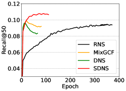
(a) Taobao, NGCF

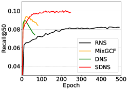
(b) Tmall, NGCF

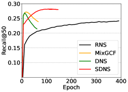
(c) Gowalla, NGCF

Figure 6. SDNS, DNS, MixGCF and RNS comparison on three datasets with NGCF as the recommender.

4.2.1. Performance Comparison

The comparison results between SDNS and above baselines on three datasets are shown in Table 2. The observations are as follows:

• The proposed method SDNS consistently outperforms all the baselines on the different datasets, and improves the performance of LightGCN by $1.09\%\sim 9.14\%$ compared to the strongest baseline (underlined in Table 2).

• Three methods that belong to the class of dynamic hard sampling branch, i.e., DNS, SDNS and MixGCF, perform better than the fixed distribution sampling (i.e. RNS), and GAN-based hard samplers (i.e. IRGAN and AdvIR), revealing that dynamic hard samplers are more likely to touch informative and high-quality negatives than the other two branches.

• The relative improvements on Gowalla $1.09\%$ w.r.t. Recall@50 are not as significant as on Taobao and Tmall, $4.68\%$ and $9.14\%$ respectively, which may be attributed to their different data structures, since Taobao and Tmall are e-commerce related but Gowalla is for social network. In fact, for Gowalla, the performances of all baselines vary by a relatively small margin.

4.2.2. Robustness analysis

Based on the second observation above, we then take a closer look at the training progress of DNS, SDNS and MixGCF respectively, with LightGCN as the underlying recommendation model. Corresponding training curves on three datasets are drawn in Figure 4, where we use RNS as a benchmark. As can be seen, SDNS converges faster than RNS, and is trained more stably than DNS and MixGCF on all datasets. The latter demonstrates better robustness of SDNS towards potential false negative samples in recommendation tasks discussed in Section 3, indicating the superiorities of SDNS in terms of effectiveness and robustness simultaneously.

4.2.3. Hardness study

In Figure 5, we conduct hardness study on Taobao, Tmall and Gowalla by changing the hardness level $H$, i.e., the size of negative candidate pool, and then investigate its influences on the behavior of SDNS and DNS, respectively. Note that the larger the $H$, the harder the negative sampled. Especially, when $H=1$, DNS will degenerate into RNS. From Figure 5, we have the following observations:

• For Taobao and Tmall, both DNS and SDNS manifest the same trend with the increase of $H$, that is, reaching the peak (when $H=16$) and then suffering from degradation ($H=32$ and $64$). Such a phenomenon is consistent with our discussion about false negatives in Section 3, i.e., harder negatives are more likely to be the false negatives, which will confuse the recommender during training procedure. As for Gowalla, due to the larger set of users and items, harder negatives ($H=64$) are preferred for model optimization.

• SDNS outperforms DNS by a large margin under different $H$ settings, indicating the better capacity of SDNS to capture reliable and high-quality negatives.

4.2.4. NGCF experiment

To verify the general effectiveness and robustness of SDNS on other GNN-based recommenders, we replace LightGCN with another popular graph collaborative filtering model, NGCF, as the basic recommender for more experiments. As shown in Figure 6, the training curves of SDNS and three representative baselines (RNS, DNS, MixGCF) under the recommender NGCF follow the similar pattern with those under LightGCN (Figure 4). In addition, SDNS still yields the best performance w.r.t. Recall and NDCG on all three datasets (Figure 6), which means SDNS, as a strong hard negative sampler, can be plugged into other GNN-based recommenders for more accurate personalized prediction.

5. Related work

In order to obtain high-quality negatives in implicit CF, several recent efforts work on hard negative samplers via emphasizing those with large matching scores (Ding et al., 2020; Rendle and Freudenthaler, 2014; Huang et al., 2020). For example, IRGAN (Wang et al., 2017) and AdvIR (Park and Chang, 2019) are two GAN-based samplers. IRGAN applies generative adversarial net to play a minimax game, where the generator acts as a recommender sampler to fool the discriminator (Wang et al., 2017). AdvIR combines adversarial negative sampling and adversarial training to generate informative instances (Park and Chang, 2019). Nevertheless, GAN-based samplers are unfit for modern recommendation since they normally require a large time complexity.

The model proposed in this paper falls into another class of hard negative techniques, i.e., dynamic hard sampling, including numerous state-of-the-arts like DNS (Rendle and Freudenthaler, 2014), SRNS (Ding et al., 2020) and MixGCF (Huang et al., 2021). SRNS first observes that both hard negatives and false negatives are assigned to high scores, yet false negatives have lower score variances relatively. Thus, SRNS avoids false negatives in implicit CF by favouring high-scored high-variance items (Ding et al., 2020), whereas variances of scores are computationally expensive. Besides, MixGCF synthesizes item embeddings and selects the one with highest score, and DNS directly chooses the highest-scored existing item. Both DNS and MixGCF show great performance regarding training effectiveness and efficiency, however, they are subjected to over-fitting problem. In this paper, on top of the basic idea of DNS, we describe a novel technique to alleviate over-fitting and enhance performance simultaneously.

Recently, some novel negative sampling techniques emerging in contrastive learning (Kalantidis et al., 2020; Shen et al., 2022; Zhang et al., 2022) inspire our work. Developed from $mixup$ technique (Zhang et al., 2018), recent studies in contrastive learning (Kalantidis et al., 2020; Shen et al., 2022; Zhang et al., 2022) prefer to synthesize novel examples by mixing information of multiple instances to generate negatives. Particularly, MoCHi derives negative embeddings by both mixing hard negative pairs as well as injecting positive information into negatives, resulting in the generalization improvement in visual feature learning (Kalantidis et al., 2020). Later, MixGCF borrows the idea of positive mixing in MoCHi to synthesizes negatives for implicit CF task (Huang et al., 2021). Both MoCHi and MixGCF incorporate positive information into hard negatives for generating harder ones, while the rationality behind remains unclear because it oftentimes couples with other techniques for better performance. In this paper, we deeply investigate why positive information is critical in hard negative synthesizing.

6. Conclusion

In this work, we propose a novel hard negative sampling strategy SDNS to empower state-of-the-art GNN-based recommenders in implicit CF task. SDNS can be easily plugged into various recommenders to improve personalized recommendation accuracy. SDNS can significantly alleviate over-fitting caused by incorrect selection of false negatives in hard negative sampling process. Extensive experiments on three datasets demonstrate the superiorities of SDNS in terms of both effectiveness and robustness.

The main idea of SDNS, i.e., positive mixing, comes from contrastive learning, a popular research line of self-supervised learning. In future work, we will attempt to transfer advanced knowledges between these two fields and try providing a unified framework.

References

- (1)
- Ding et al. (2019) Jingtao Ding, Yuhan Quan, Xiangnan He, Yong Li, and Depeng Jin. 2019. Reinforced Negative Sampling for Recommendation with Exposure Data. In Proceedings of the Twenty-Eighth International Joint Conference on Artificial Intelligence, IJCAI 2019, Macao, China, August 10-16, 2019. 2230–2236.
- Ding et al. (2020) Jingtao Ding, Yuhan Quan, Quanming Yao, Yong Li, and Depeng Jin. 2020. Simplify and Robustify Negative Sampling for Implicit Collaborative Filtering. In Advances in Neural Information Processing Systems 33: Annual Conference on Neural Information Processing Systems 2020, NeurIPS 2020, December 6-12, 2020, virtual.
- Dziugaite and Roy (2015) Gintare Karolina Dziugaite and Daniel M. Roy. 2015. Neural Network Matrix Factorization. CoRR (2015).
- He et al. (2020) Xiangnan He, Kuan Deng, Xiang Wang, Yan Li, Yong-Dong Zhang, and Meng Wang. 2020. LightGCN: Simplifying and Powering Graph Convolution Network for Recommendation. In Proceedings of the 43rd International ACM SIGIR conference on research and development in Information Retrieval, SIGIR 2020, Virtual Event, China, July 25-30, 2020. 639–648.
- Huang et al. (2020) Jui-Ting Huang, Ashish Sharma, Shuying Sun, Li Xia, David Zhang, Philip Pronin, Janani Padmanabhan, Giuseppe Ottaviano, and Linjun Yang. 2020. Embedding-based Retrieval in Facebook Search. In KDD ’20: The 26th ACM SIGKDD Conference on Knowledge Discovery and Data Mining, Virtual Event, CA, USA, August 23-27, 2020. 2553–2561.
- Huang et al. (2021) Tinglin Huang, Yuxiao Dong, Ming Ding, Zhen Yang, Wenzheng Feng, Xinyu Wang, and Jie Tang. 2021. MixGCF: An Improved Training Method for Graph Neural Network-based Recommender Systems. In KDD ’21: The 27th ACM SIGKDD Conference on Knowledge Discovery and Data Mining, Virtual Event, Singapore, August 14-18, 2021, Feida Zhu, Beng Chin Ooi, and Chunyan Miao (Eds.). ACM, 665–674. https://doi.org/10.1145/3447548.3467408
- Kalantidis et al. (2020) Yannis Kalantidis, Mert Bülent Sariyildiz, Noé Pion, Philippe Weinzaepfel, and Diane Larlus. 2020. Hard Negative Mixing for Contrastive Learning. In Advances in Neural Information Processing Systems 33: Annual Conference on Neural Information Processing Systems 2020, NeurIPS 2020, December 6-12, 2020, virtual.
- Koren (2008) Yehuda Koren. 2008. Factorization meets the neighborhood: a multifaceted collaborative filtering model. In Proceedings of the 14th ACM SIGKDD International Conference on Knowledge Discovery and Data Mining, Las Vegas, Nevada, USA, August 24-27, 2008. 426–434.
- Koren et al. (2009) Yehuda Koren, Robert M. Bell, and Chris Volinsky. 2009. Matrix Factorization Techniques for Recommender Systems. Computer 42, 8 (2009), 30–37.
- Liang et al. (2016) Dawen Liang, Laurent Charlin, James McInerney, and David M Blei. 2016. Modeling user exposure in recommendation. In Proceedings of the 25th international conference on World Wide Web. 951–961.
- Park and Chang (2019) Dae Hoon Park and Yi Chang. 2019. Adversarial Sampling and Training for Semi-Supervised Information Retrieval. In The World Wide Web Conference, WWW 2019, San Francisco, CA, USA, May 13-17, 2019. 1443–1453.
- Rendle and Freudenthaler (2014) Steffen Rendle and Christoph Freudenthaler. 2014. Improving pairwise learning for item recommendation from implicit feedback. In Seventh ACM International Conference on Web Search and Data Mining, WSDM 2014, New York, NY, USA, February 24-28, 2014. 273–282.
- Rendle et al. (2009) Steffen Rendle, Christoph Freudenthaler, Zeno Gantner, and Lars Schmidt-Thieme. 2009. BPR: Bayesian Personalized Ranking from Implicit Feedback. In UAI 2009, Proceedings of the Twenty-Fifth Conference on Uncertainty in Artificial Intelligence, Montreal, QC, Canada, June 18-21, 2009. 452–461.
- Salakhutdinov and Mnih (2007) Ruslan Salakhutdinov and Andriy Mnih. 2007. Probabilistic Matrix Factorization. In Advances in Neural Information Processing Systems 20, Proceedings of the Twenty-First Annual Conference on Neural Information Processing Systems, Vancouver, British Columbia, Canada, December 3-6, 2007. 1257–1264.
- Shen et al. (2022) Zhiqiang Shen, Zechun Liu, Zhuang Liu, Marios Savvides, Trevor Darrell, and Eric Po Xing. 2022. Un-mix: Rethinking Image Mixtures for Unsupervised Visual Representation Learning. In Thirty-Sixth AAAI Conference on Artificial Intelligence, AAAI 2022, Thirty-Fourth Conference on Innovative Applications of Artificial Intelligence, IAAI 2022, The Twelveth Symposium on Educational Advances in Artificial Intelligence, EAAI 2022 Virtual Event, February 22 - March 1, 2022. 2216–2224.
- van den Berg et al. (2017) Rianne van den Berg, Thomas N. Kipf, and Max Welling. 2017. Graph Convolutional Matrix Completion. CoRR abs/1706.02263 (2017).
- Wang et al. (2017) Jun Wang, Lantao Yu, Weinan Zhang, Yu Gong, Yinghui Xu, Benyou Wang, Peng Zhang, and Dell Zhang. 2017. IRGAN: A Minimax Game for Unifying Generative and Discriminative Information Retrieval Models. In Proceedings of the 40th International ACM SIGIR Conference on Research and Development in Information Retrieval, Shinjuku, Tokyo, Japan, August 7-11, 2017. 515–524.
- Wang et al. (2019a) Xiang Wang, Xiangnan He, Yixin Cao, Meng Liu, and Tat-Seng Chua. 2019a. KGAT: Knowledge Graph Attention Network for Recommendation. In Proceedings of the 25th ACM SIGKDD International Conference on Knowledge Discovery & Data Mining, KDD 2019, Anchorage, AK, USA, August 4-8, 2019. 950–958.
- Wang et al. (2019b) Xiang Wang, Xiangnan He, Meng Wang, Fuli Feng, and Tat-Seng Chua. 2019b. Neural Graph Collaborative Filtering. In Proceedings of the 42nd International ACM SIGIR Conference on Research and Development in Information Retrieval, SIGIR 2019, Paris, France, July 21-25, 2019. 165–174.
- Ying et al. (2018) Rex Ying, Ruining He, Kaifeng Chen, Pong Eksombatchai, William L. Hamilton, and Jure Leskovec. 2018. Graph Convolutional Neural Networks for Web-Scale Recommender Systems. In Proceedings of the 24th ACM SIGKDD International Conference on Knowledge Discovery & Data Mining, KDD 2018, London, UK, August 19-23, 2018. 974–983.
- Zhang et al. (2018) Hongyi Zhang, Moustapha Cissé, Yann N. Dauphin, and David Lopez-Paz. 2018. mixup: Beyond Empirical Risk Minimization. In 6th International Conference on Learning Representations, ICLR 2018, Vancouver, BC, Canada, April 30 - May 3, 2018, Conference Track Proceedings.
- Zhang and Chen (2020) Muhan Zhang and Yixin Chen. 2020. Inductive Matrix Completion Based on Graph Neural Networks. In 8th International Conference on Learning Representations, ICLR 2020, Addis Ababa, Ethiopia, April 26-30, 2020.
- Zhang et al. (2022) Shaofeng Zhang, Meng Liu, Junchi Yan, Hengrui Zhang, Lingxiao Huang, Xiaokang Yang, and Pinyan Lu. 2022. M-Mix: Generating Hard Negatives via Multi-sample Mixing for Contrastive Learning. In KDD ’22: The 28th ACM SIGKDD Conference on Knowledge Discovery and Data Mining, Washington, DC, USA, August 14 - 18, 2022. 2461–2470.