Geodesic continued fraction for Shimura curves and its periodicity: the case of $(2,3,7)$-triangle group

Abstract

In this paper we study the geodesic continued fraction in the case of the Shimura curve coming from the $(2,3,7)$-triangle group. We construct a certain continued fraction expansion of real numbers using the so-called coding of the geodesics on the Shimura curve, and prove the Lagrange type periodicity theorem for the expansion which captures the fundamental relative units of quadratic extensions of $\mathbb{Q}(\cos(2\pi/7))$ with rank one relative unit groups. We also discuss the convergence of these continued fractions.

Keywords: continued fraction; Shimura curve; (2,3,7)-triangle group; Lagrange’s theorem; unit group

2020 Mathematics Subject Classification: 11A55, 11R27.

1 Introduction

Let $\eta:=2\cos\left(\frac{2\pi}{7}\right)\in\mathbb{R}$ be the unique positive root of $X^{3}+X^{2}-2X-1$. The aim of this paper is to present a geometric construction of the continued fraction expansion such as

$$(1-\eta^{2})\sqrt{\eta}+\sqrt{1+3\eta-2\eta^{2}}$$

$$=(1-\eta^{2})\sqrt{\eta}+\eta^{2}-\eta+\cfrac{2(1+2\eta-2\eta^{2})}{\eta^{2}-\eta+\cfrac{1+2\eta-2\eta^{2}}{\eta^{2}-\eta+\cfrac{1+2\eta-2\eta^{2}}{\eta^{2}-\eta+\cfrac{1+2\eta-2\eta^{2}}{\cdots{\text{(}periodic)}}}}}$$ (1.1)

with the Lagrange type periodicity property (Theorem 3.4.1 and Theorem 3.4.5). Here the term $(1-\eta^{2})\sqrt{\eta}$ on the both sides should not be deleted in order for this continued fraction expansion to have the natural geometric meaning. See Example 3.6.2.

The classical Lagrange theorem in the theory of continued fraction says that the continued fraction expansion of a given real number becomes periodic if and only if the number is a real quadratic irrational, and that the period of the continued fraction expansion describes the fundamental unit of the associated order in the real quadratic field. Analogously, we know that a given geodesic on the upper-half plane $\mathfrak{h}$ becomes a closed geodesic (“periodic”) on the modular curve $SL_{2}(\mathbb{Z})\backslash\mathfrak{h}$ if and only if the two end points of the geodesic are conjugate real quadratic irrationals, and that the length of the closed geodesic becomes the regulator of the associated order in the real quadratic field. Cf. Theorem 2.1.1.

Our motivation for this study is to extend the Lagrange theorem to number fields other than real quadratic fields based on this geometric analogue of the Lagrange theorem. In a previous paper [bekki17], based on this analogy and inspired by the works of Artin [artin24], Sarnak [sarnak82], Series [series85], Katok [katok96], Lagarias [lagarias94], Beukers [beukers14], etc., we have studied the geodesic multi-dimensional continued fraction and its periodicity using the geodesics on the locally symmetric space of $SL_{n}$. As a result we have established a geodesic multi-dimensional continued fraction and a $p$-adelic continued fraction with the Lagrange type periodicity theorems in the case of extensions $E/F$ of number fields with rank one relative unit group, and in the case of imaginary quadratic fields with rank one $p$-unit group, respectively. Recently the author found that Vulakh [vulakh02], [vulakh04] had also used the same idea to compute the fundamental units of some families of number fields.

In this paper we mainly study the case of the Shimura curve coming from the $(2,3,7)$-triangle group $\Delta(2,3,7)$. We construct a continued fraction expansion using the geodesics on the Shimura curve $\Delta(2,3,7)\backslash\mathfrak{h}$, and prove the Lagrange type periodicity theorem for quadratic extensions $K/\mathbb{Q}(\cos(2\pi/7))$ with rank one relative unit groups. We refer to such an extension the “relative rank one” extension. Although these number fields can already be treated in the previous paper [bekki17], a major difference is that we can actually expand numbers in the form of “continued fraction” as in (1.1), while the geodesic multi-dimensional continued fraction in [bekki17] only gives a sequence of matrices in $SL_{n}(\mathbb{Z})$.

The idea of considering the geodesic continued fraction for some arithmetic Fuchsian groups is briefly discussed in [katok86] by Katok. In the final sections (Remark and Examples) of [katok86], Katok considers the arithmetic groups coming from quaternion algebras over $\mathbb{Q}$, and gives some examples of the periodic geodesic continued fraction expansions (Katok calls this the “code”) of closed geodesics. Some of the essential ideas in this paper are generalization of Katok’s ideas to our case of quaternion algebras over totally real fields $F$, especially $\mathbb{Q}(\cos(2\pi/7))$.

Our strategy is as follows. First we extend the geometric analogue of the Lagrange theorem (Theorem 2.1.1) to Shimura curves (Proposition 2.2.2). We treat a general Shimura curve, not only the one coming from the $(2,3,7)$-triangle group, since the argument does not change too much. Then we restrict ourselves to the Shimura curve $\Delta(2,3,7)\backslash\mathfrak{h}$ and construct the continued fraction expansion which can detect the relative units of the relative rank one quadratic extensions of $\mathbb{Q}(\cos(2\pi/7))$ as the periods of the continued fraction expansion.

For this purpose, we use the technique called the geodesic continued fraction studied by Series [series85], Katok [katok96], etc. in the field of reduction theory, dynamical systems, etc. (Some authors refer to the geodesic continued fraction also as the cutting sequence or the Morse coding.) In order to obtain a convergent continued fraction expansion which is similar to the classical one such as (1.1), we slightly modify the original algorithm by considering the regular geodesic heptagon which is the union of some copies of the fundamental domain. Here we use the generator of $\Delta(2,3,7)$ given by Elkies [elkies98], Katz-Schaps-Vishne [katzschapsvishne11]. See Figure 1 and Definition 3.2.5. Then we consider the formal continued fraction expansion (3.9) associated to the geodesic continued fraction, and discuss its convergence. In fact, although the traditional $k$-th convergent of (3.9) does not converge in general, we show that there is a natural regularization of the $k$-th convergent and prove its convergence. See Theorem 3.3.2, Corollary 3.3.3 and Corollary 3.3.4.

Finally we study the Lagrange type periodicity of our continued fraction expansion. We prove two versions of the periodicity theorem: the first version Theorem 3.4.1 is about the closed geodesics on the Shimura curve $\Delta(2,3,7)\backslash\mathfrak{h}$, and the second refined version Theorem 3.4.5 is about geodesics not necessarily closed on $\Delta(2,3,7)\backslash\mathfrak{h}$. Note that it is a well known fact that the geodesic continued fraction (or the cutting sequence/Morse code) of a “generic” geodesic becomes periodic if and only if the geodesic becomes closed geodesic on the quotient space. Cf. Katok-Ugarcovici [katokugarcovici07]*p.94. Therefore, (1) of Theorem 3.4.1, i.e., the periodicity of the geodesic continued fraction expansion itself, follows naturally from Proposition 2.2.2 and this fact. On the other hand, we need more argument for the latter part of Theorem 3.4.1 about the fundamental unit. Actually, we have to take care about the vertices of the fundamental domain in order to obtain the fundamental units as a minimal period of the continued fraction expansions. We also need some delicate arguments for the periodicity in Theorem 3.4.5. See also Remark 3.4.6.

Remark on some relevant preceding studies

There are many literatures which study the closed geodesics on hyperbolic surfaces (not necessarily Shimura curves) using the periodic geodesic continued fractions or the cutting sequences/Morse codes.

For example, in [series86], [katok86], [abramskatok19], Series, Katok and Abrams-Katok study the reduction theory for the general Fuchsian groups or the symbolic dynamics associated to the geodesic flows on hyperbolic sufaces using the cutting sequence for (certain classes of) Fuchsian groups. As we have mentioned above, in [katok86], Katok considers the case where the Fuchsian group is coming from the quaternion algebras over $\mathbb{Q}$. Some new features in this paper are to give the continued fraction expression such as (3.9) and to establish an explicit correspondence between the period of continued fraction expansions and the fundamental relative unit of certain quadratic extensions over the totally real field $\mathbb{Q}(\cos(2\pi/7))$.

As another example, in [vogeler03], Vogeler studies the closed geodesics on the Hurwitz surface ($=\Delta(2,3,7)\backslash\mathfrak{h}$). He associates each “edge path” the hyperbolic element in the $(2,3,7)$-triangle group $\Delta(2,3,7)$, and hence the geodesic on $\mathfrak{h}$ which becomes closed on $\Delta(2,3,7)\backslash\mathfrak{h}$. On the other hand the “edge path” admits a very simple combinatorial description using the words consisting of $R$ and $L$. Using this correspondence, he combinatorially studies the length spectra of closed geodesics on $\Delta(2,3,7)\backslash\mathfrak{h}$. In this paper, we basically study the reverse direction, that is, we input the geodesics (not necessarily closed) and output the $RL$-sequences or the hyperbolic elements if the geodesic continued fraction becomes periodic, and discuss its relation to unit groups of the quadratic extension of $\mathbb{Q}(\cos(2\pi/7))$.

To sum up, the upshots of this paper are

1. to give a new explicit presentation of any real number as a “convergent” continued fraction such as (1.1) or (3.9) which becomes periodic if and only if the number is a certain algebraic number, and

2. to establish the correspondence between the periods of such continued fractions and the fundamental relative units of the “relative rank one” extensions of $\mathbb{Q}(\cos(2\pi/7))$,

by using the arithmetic and geometric properties of the Shimura curve $\Delta(2,3,7)\backslash\mathfrak{h}$.

2 Preliminaries on Shimura curves

Let $F$ be a totally real number field of degree $d\geq 1$ and let $\mathcal{O}_{F}$ be the ring of integers of $F$. We denote by $\sigma_{1},\dots,\sigma_{d}$ the set of archimedean places of $F$. We also denote by $\sigma_{i}:F\hookrightarrow F_{\sigma_{i}}:=\mathbb{R}$ $(1\leq i\leq d)$ the completion map of $F$ at $\sigma_{i}$. Let $A$ be a quaternion algebra over $F$ and let $\mathcal{O}\subset A$ be a maximal order, i.e., an $\mathcal{O}_{F}$-subalgebra of $A$ which is finitely generated as an $\mathcal{O}_{F}$-module such that $\mathcal{O}\otimes_{\mathcal{O}_{F}}F=A$, and not properly contained in any other such $\mathcal{O}_{F}$-subalgebra. We denote by $\mathcal{O}^{1}:=\{x\in\mathcal{O}^{\times}\mid\mathop{\mathrm{nrd}}\nolimits(x)=1\}$ the group of reduced norm one units in $\mathcal{O}$, where $\mathop{\mathrm{nrd}}\nolimits:A\rightarrow F$ is the reduced norm on $A$. Suppose that $A$ is unramified at $\sigma_{1}$ and ramified at $\sigma_{2},\dots,\sigma_{d}$, i.e., $A\otimes_{F}F_{\sigma_{1}}\simeq M_{2}(F_{\sigma_{1}})$ and $A\otimes_{F}F_{\sigma_{i}}\simeq\mathbb{H}$ (the Hamilton quaternion) for $i=2,\dots,d$. Let us fix such an isomorphism (as $F_{\sigma_{1}}$-algebras)

$$\iota:A\otimes_{F}F_{\sigma_{1}}\overset{\sim}{\rightarrow}M_{2}(F_{\sigma_{1}})=M_{2}(\mathbb{R}),$$ (2.1)

and set $\Gamma_{\mathcal{O}}:=\iota(\mathcal{O}^{1})$. By the definition of the reduced norm, $\Gamma_{\mathcal{O}}$ is a subgroup of $SL_{2}(\mathbb{R})$ and acts on the upper-half plane by the linear fractional transformation.

To be precise, we denote by $\mathfrak{h}:=\{z=x+\sqrt{-1}y\in\mathbb{C}\mid\operatorname{Im}(z)=y>0\}\subset\mathbb{C}$ the upper-half plane. We naturally embed $\mathfrak{h}$ into $\mathbb{P}^{1}(\mathbb{C}):=\mathbb{C}\cup\{\infty\}$, the complex projective line with the usual topology as a manifold. Then the boundary $\partial\mathfrak{h}$ of $\mathfrak{h}$ in $\mathbb{P}^{1}(\mathbb{C})$ becomes $\mathbb{P}^{1}(\mathbb{R}):=\mathbb{R}\cup\{\infty\}$, and we denote by $\overline{\mathfrak{h}}:=\mathfrak{h}\cup\mathbb{P}^{1}(\mathbb{R})$ the compactified upper-half plane in $\mathbb{P}^{1}(\mathbb{C})$. The group $GL_{2}(\mathbb{R})$ acts on $\mathbb{P}^{1}(\mathbb{C})$ by the linear fractional transformation:

$$\gamma z=\frac{az+b}{cz+d}\quad\text{ for}\quad\gamma=\begin{pmatrix}a&b\\ c&d\\ \end{pmatrix}\in GL_{2}(\mathbb{R}),z\in\mathbb{P}^{1}(\mathbb{C}),$$ (2.2)

and the action of $SL_{2}(\mathbb{R})$ preserves $\mathfrak{h}$ and $\mathbb{P}^{1}(\mathbb{R})$. Thus $SL_{2}(\mathbb{R})$ also acts on $\mathfrak{h}$ and $\mathbb{P}^{1}(\mathbb{R})$ by the linear fractional transformation. We also equip $\mathfrak{h}$ with the Poincaré metric $ds^{2}=\frac{dx^{2}+dy^{2}}{y^{2}}$ ($z=x+\sqrt{-1}y\in\mathfrak{h}$). The action of $SL_{2}(\mathbb{R})$ on $\mathfrak{h}$ is preserves this metric, and hence preserves the geodesics on $\mathfrak{h}$.

Then it is known that $\Gamma_{\mathcal{O}}$ acts properly discontinuously on $\mathfrak{h}$, and the quotient space $\Gamma_{\mathcal{O}}\backslash\mathfrak{h}$ has a canonical structure of an algebraic curve over $\overline{\mathbb{Q}}$. See Shimura [shimura67]. Algebraic curves obtained in this way are called the Shimura curves (of level 1).

In the following, for $\alpha,\beta\in\mathbb{P}^{1}(\mathbb{R})=\mathbb{R}\cup\{\infty\}$ such that $\alpha\neq\beta$, we mean by the oriented geodesic on $\mathfrak{h}$ joining $\beta$ to $\alpha$ the geodesic on $\mathfrak{h}$ joining $\alpha$ and $\beta$ equipped with the orientation from $\beta$ to $\alpha$, and denote by $\varpi_{\beta\to\alpha}$.

2.1 The modular curve

In this subsection we recall the case of the modular curve $SL_{2}(\mathbb{Z})\backslash\mathfrak{h}$ as an example of Shimura curve and explain the geometric interpretation of the Lagrange theorem which is the key idea for our generalization of the Lagrange theorem.

We consider the case where $F=\mathbb{Q},A=M_{2}(\mathbb{Q})$ and $\mathcal{O}=M_{2}(\mathbb{Z})\subset A$. We choose the canonical base change isomorphism $\iota=\mathop{\mathrm{id}}\nolimits:M_{2}(\mathbb{Q})\otimes\mathbb{R}\simeq M_{2}(\mathbb{R})$ as an identification (2.1). Then we have $\Gamma_{\mathcal{O}}=SL_{2}(\mathbb{Z})$ and the resulting Shimura curve $\Gamma_{\mathcal{O}}\backslash\mathfrak{h}=SL_{2}(\mathbb{Z})\backslash\mathfrak{h}$ is the classical modular curve. Then the following is known about the closed geodesics on the modular curve $SL_{2}(\mathbb{Z})\backslash\mathfrak{h}$. See Sarnak [sarnak82] for example.

Theorem 2.1.1 (The geodesic Lagrange theorem).

1. Let $\alpha,\beta\in\mathbb{R}\cup\{\infty\}=\partial\mathfrak{h}$ such that $\alpha\neq\beta$, and let $\varpi$ be the oriented geodesic on the upper-half plane $\mathfrak{h}$ joining $\beta$ to $\alpha$. We denote by $\overline{\varpi}$ the projection of the geodesic $\varpi$ on the modular curve. The following conditions are equivalent.

   1. The projected geodesic $\overline{\varpi}$ becomes a closed geodesic, i.e., $\overline{\varpi}$ has a compact image in $SL_{2}(\mathbb{Z})\backslash\mathfrak{h}$.

   2. There exists a hyperbolic element $\gamma\in SL_{2}(\mathbb{Z})$ (i.e., $\gamma$ has two distinct real eigenvalues) such that $\gamma\varpi=\varpi$, i.e., $\gamma\alpha=\alpha$ and $\gamma\beta=\beta$.

   3. The end points $\alpha,\beta$ are real quadratic irrationals conjugate to each other over $\mathbb{Q}$.

2. Suppose that the above conditions are satisfied. Let $\Gamma_{\varpi}:=\{\gamma\in SL_{2}(\mathbb{Z})\mid\gamma\varpi=\varpi\}$ be the stabilizer subgroup of $\varpi$ in $SL_{2}(\mathbb{Z})$, and define an order $\mathcal{O}_{\alpha}$ in the real quadratic field $\mathbb{Q}(\alpha)$ by $\mathcal{O}_{\alpha}:=\{x\in\mathbb{Q}(\alpha)\mid x(\mathbb{Z}\alpha+\mathbb{Z})\subset(\mathbb{Z}\alpha+\mathbb{Z})\}$. We denote by $\mathcal{O}_{\alpha}^{1}:=\{x\in\mathcal{O}_{\alpha}^{\times}\mid N_{\mathbb{Q}(\alpha)/\mathbb{Q}}(x)=1\}$ the group of norm one units. Then the following natural map is an isomorphism of groups.

   $$\Gamma_{\varpi}\overset{\sim}{\rightarrow}\mathcal{O}_{\alpha}^{1};\begin{pmatrix}a&b\\ c&d\\ \end{pmatrix}\mapsto c\alpha+d.$$ (2.3)

Recall that the classical Lagrange theorem says that the continued fraction expansion of a real number $\alpha$ becomes periodic if and only if $\alpha$ is a real quadratic irrational, and we can actually compute the fundamental unit of $\mathcal{O}_{\alpha}$ from the period of continued fraction expansion of $\alpha$. Therefore, Theorem 2.1.1 can be seen as a geometric interpretation of the Lagrange theorem.

In the following we first extend Theorem 2.1.1 to the Shimura curves $\Gamma_{\mathcal{O}}\backslash\mathfrak{h}$ explicitly (Proposition 2.2.2). Then we restrict ourselves to the special case where $\Gamma_{\mathcal{O}}$ becomes the so called $(2,3,7)$-triangle group, and construct our continued fraction explicitly. We first discuss the convergence of the continued fraction expansion, and then deduce the Lagrange type periodicity theorem from Proposition 2.2.2.

2.2 Closed geodesics on Shimura curves

Now we return to the general setting and use the notations in the beginning of Section 2, i.e., $F$ is a totally real field of degree $d$, $A$ is a quaternion algebra over $F$ such that $A\otimes_{\mathbb{Q}}\mathbb{R}\simeq M_{2}(\mathbb{R})\times\mathbb{H}^{d-1}$, $\mathcal{O}\subset A$ is a maximal order of $A$, etc. In the following we also assume that $A\not\simeq M_{2}(F)$ (hence $A$ is a division algebra), since the case where $A\simeq M_{2}(F)$ has already explained in the previous subsection. (Note that if $A\simeq M_{2}(F)$ then $F$ must be $\mathbb{Q}$ by the assumption $A\otimes_{\mathbb{Q}}\mathbb{R}\simeq M_{2}(\mathbb{R})\times\mathbb{H}^{d-1}$.)

For simplicity, we regard $F$ as a subfield of $\mathbb{R}$ via the embedding $\sigma_{1}:F\hookrightarrow F_{\sigma_{1}}=\mathbb{R}$. In order to extend Theorem 2.1.1 we fix the identification $\iota:A\otimes_{F}\mathbb{R}\overset{\sim}{\rightarrow}M_{2}(\mathbb{R})$ (2.1) explicitly as follows. Since $\mathop{\mathrm{char}}\nolimits F=0\neq 2$, the quaternion algebra $A$ is isomorphic to $\left(\dfrac{a,b}{F}\right)$ for some $a,b\in F^{\times}$. Here $\left(\dfrac{a,b}{F}\right)$ is the quaternion algebra generated by the basis $1,i,j,k$ of the following form.

$$\left(\dfrac{a,b}{F}\right)=F+Fi+Fj+Fk$$ (2.4)

$$~{}~{}i^{2}=a,j^{2}=b,ij=-ji=k.$$ (2.5)

By the assumptions $A\not\simeq M_{2}(F)$ and $A\otimes_{F}\mathbb{R}\simeq M_{2}(\mathbb{R})$, we have $a,b\notin(F^{\times})^{2}$ and we may assume $a,b>0$. We take a splitting field $L:=F(\sqrt{b})\subset\mathbb{R}$. For $z\in L$ we denote by $\bar{z}$ the conjugate of $z$ over $F$, i.e.,

$$\bar{~{}}:L\rightarrow L;z=x+y\sqrt{b}\mapsto\bar{z}=x-y\sqrt{b}\quad(x,y\in F).$$ (2.6)

Then we have an embedding

$$\iota:A\simeq\left(\dfrac{a,b}{F}\right)\hookrightarrow M_{2}(L)\subset M_{2}(\mathbb{R});\begin{cases}1&\mapsto\begin{pmatrix}1&0\\ 0&1\\ \end{pmatrix}\vspace{1mm}\\ i&\mapsto\begin{pmatrix}0&a\\ 1&0\\ \end{pmatrix}\vspace{1mm}\\ j&\mapsto\begin{pmatrix}\sqrt{b}&0\\ 0&-\sqrt{b}\\ \end{pmatrix}\end{cases}$$ (2.7)

as $F$-algebras which induces an isomorphism $\iota:A\otimes_{F}\mathbb{R}\overset{\sim}{\rightarrow}M_{2}(\mathbb{R})$. Note that the image of $A$ under $\iota$ can be described as follows:

$$\iota:A\overset{\sim}{\rightarrow}\left\{\left.\begin{pmatrix}z&a\bar{w}\\ w&\bar{z}\end{pmatrix}\right|z,w\in L\right\}\subset M_{2}(L).$$ (2.8)

In the following we regard $A$ as a subalgebra of $M_{2}(L)$ via this identification. Then the reduced norm and the reduced trace on $A$ is nothing but the restriction of the determinant and the trace on $M_{2}(L)$ respectively, i.e.,

$$\mathop{\mathrm{nrd}}\nolimits=\det: A\rightarrow F;\begin{pmatrix}z&a\bar{w}\\ w&\bar{z}\end{pmatrix}\mapsto z\bar{z}-aw\bar{w},$$ (2.9)

$$\mathop{\mathrm{trd}}\nolimits=\mathop{\mathrm{tr}}\nolimits: A\rightarrow F;\begin{pmatrix}z&a\bar{w}\\ w&\bar{z}\end{pmatrix}\mapsto z+\bar{z}.$$ (2.10)

Now let $\alpha,\beta\in\mathbb{R}\cup\{\infty\}=\partial\mathfrak{h}$ such that $\alpha\neq\beta$, and let $\varpi_{\beta\to\alpha}$ be the oriented geodesic on $\mathfrak{h}$ joining $\beta$ to $\alpha$. We denote by $\overline{\varpi}_{\beta\to\alpha}$ the projection of $\varpi_{\beta\to\alpha}$ on the Shimura curve $\Gamma_{\mathcal{O}}\backslash\mathfrak{h}$. Let

$$\Gamma_{\varpi_{\beta\to\alpha}}:=\{\gamma\in\Gamma_{\mathcal{O}}\mid\gamma\varpi_{\beta\to\alpha}=\varpi_{\beta\to\alpha}\text{, i.e., }\gamma\alpha=\alpha\text{ and }\gamma\beta=\beta\}$$ (2.11)

be the stabilizer subgroup of $\varpi_{\beta\to\alpha}$ in $\Gamma_{\mathcal{O}}$. We recall the following elementary fact.

Lemma 2.2.1.

An element $\gamma\in\Gamma_{\varpi_{\beta\to\alpha}}$ is a hyperbolic element (i.e., an element with distinct real eigenvalues) if and only if $\gamma\neq\pm 1$.

Proof.

Let $\gamma\in\Gamma_{\varpi_{\beta\to\alpha}}$. First note that $\gamma$ is diagonalizable in $M_{2}(\mathbb{R})$ since it has two distinct fixed points $\alpha,\beta\in\mathbb{P}^{1}(\mathbb{R})$. More precisely, let

$$v=\begin{pmatrix}\alpha_{1}\\ \alpha_{2}\end{pmatrix},\ w=\begin{pmatrix}\beta_{1}\\ \beta_{2}\end{pmatrix}\in\mathbb{R}^{2}\!-\!\{0\},$$ (2.12)

be the eigenvectors of $\gamma$ corresponding to the distinct fixed points $\alpha$, $\beta$ respectively, i.e., $\alpha=[\alpha_{1}:\alpha_{2}],\beta=[\beta_{1}:\beta_{2}]$ in $\mathbb{P}^{1}(\mathbb{R})$. Let $\lambda,\mu\in\mathbb{R}$ be the eigenvalues of $\gamma$ corresponding to $v,w$ respectively. Then we have

$$\gamma=\begin{pmatrix}\alpha_{1}&\beta_{1}\\ \alpha_{2}&\beta_{2}\end{pmatrix}\begin{pmatrix}\lambda&0\\ 0&\mu\end{pmatrix}\begin{pmatrix}\alpha_{1}&\beta_{1}\\ \alpha_{2}&\beta_{2}\end{pmatrix}^{-1}.$$ (2.13)

Now, if $\lambda=\mu$, then $\lambda=\mu=\pm 1$ since $\det\gamma=1$, and hence $\gamma=\pm 1$. Therefore, we see that $\gamma$ has distinct real eigenvalues if and only if $\gamma\neq\pm 1$. ∎

The following proposition extends Theorem 2.1.1 to the Shimura curve $\Gamma_{\mathcal{O}}\backslash\mathfrak{h}$.

Proposition 2.2.2 (The geodesic Lagrange theorem for Shimura curves).

Let the notations be as above. Then the following conditions are equivalent.

1. The projection $\overline{\varpi}_{\beta\to\alpha}$ becomes a closed geodesic, i.e., $\overline{\varpi}_{\beta\to\alpha}$ has a compact image in $\Gamma_{\mathcal{O}}\backslash\mathfrak{h}$.

2. There exists a hyperbolic element in $\Gamma_{\varpi_{\beta\to\alpha}}$, i.e., $\Gamma_{\varpi_{\beta\to\alpha}}\neq\{\pm 1\}$.

3. The two endpoints $\alpha$ and $\beta$ are of the following form:

   $$\begin{cases}\alpha&=\frac{1}{2w}(z-\bar{z}\pm\sqrt{D_{z,w}})\\ \beta&=\frac{1}{2w}(z-\bar{z}\mp\sqrt{D_{z,w}})\end{cases}$$ (2.14)

   for some $z,w\in L$ such that $D_{z,w}:=(z-\bar{z})^{2}+4aw\bar{w}>0$. Here if $w=0$, we assume $(\alpha,\beta)=(0,\infty)$ or $(\infty,0)$.

Before proving this proposition we introduce some more notations. Suppose that $\alpha,\beta\in\mathbb{R}\cup\{\infty\}$ can be written in the form

$$\alpha =\frac{1}{2w}(z-\bar{z}\pm\sqrt{D_{z,w}})$$ (2.15)

$$\beta =\frac{1}{2w}(z-\bar{z}\mp\sqrt{D_{z,w}})$$ (2.16)

for $z,w\in L$ such that $D_{z,w}=(z-\bar{z})^{2}+4aw\bar{w}>0$. Note that we have $D_{z,w}\in F$ by the definition. Set $\theta_{z,w}:=\begin{pmatrix}z&a\bar{w}\\ w&\bar{z}\\ \end{pmatrix}\in A\subset M_{2}(L)$. Then we define

$$K_{z,w}:=F[\theta_{z,w}]\subset A$$ (2.17)

to be the $F$-subalgebra of $A$ generated by $\theta_{z,w}$, and set $\mathcal{O}_{z,w}:=K_{z,w}\cap\mathcal{O}$. Note that we have $\theta_{z,w}\notin F$ because $D_{z,w}\neq 0$. We denote by $\mathcal{O}_{z,w}^{1}:=\mathcal{O}_{z,w}^{\times}\cap\mathcal{O}^{1}$ the group of reduced norm one units in $\mathcal{O}_{z,w}$.

Lemma 2.2.3.

1. The subalgebra $K_{z,w}$ is a maximal (commutative) subfield in $A$.

2. The field $K_{z,w}$ is a quadratic extension of $F$, and the reduced norm on $A$ restricted to $K_{z,w}$ coincides with the field norm of $K_{z,w}/F$.

3. The field $K_{z,w}$ splits at the place $\sigma_{1}$ and ramifies at the places $\sigma_{2},\dots,\sigma_{d}$, i.e., $K_{z,w}\otimes_{F}\mathbb{R}\simeq\mathbb{R}\times\mathbb{R}$ and $K_{z,w}\otimes_{F}F_{\sigma_{i}}\simeq\mathbb{C}$ for $2\leq i\leq d$.

4. Let $F(\sqrt{D_{z,w}})\subset\mathbb{R}$ be the quadratic extension of $F$ in $\mathbb{R}$ generated by $\sqrt{D_{z,w}}$. Then we have the following isomorphism of fields:

   $$\rho_{\alpha}:K_{z,w}\overset{\sim}{\rightarrow}F(\sqrt{D_{z,w}});\begin{pmatrix}q&r\\ s&t\\ \end{pmatrix}\mapsto s\alpha+t.$$ (2.18)

5. We have the following identity:

   $$K_{z,w}^{\times} =\{\gamma\in A^{\times}\subset GL_{2}(L)\mid\gamma\alpha=\alpha,\gamma\beta=\beta\}$$ (2.19)

   $$=\{\gamma\in A^{\times}\subset GL_{2}(L)\mid\gamma\alpha=\alpha\}$$ (2.20)

   In particular, the subfield $K_{z,w}\subset A$ depends only on $\alpha$, and does not depend on the choice of $z,w\in L$. By taking the intersection with $\mathcal{O}^{1}$ we also obtain $\mathcal{O}_{z,w}^{1}=\Gamma_{\varpi_{\beta\to\alpha}}$.

6. The subring $\mathcal{O}_{z,w}\subset K_{z,w}$ is an order in $K_{z,w}$. In particular $\mathop{\mathrm{rank}}\nolimits_{\mathbb{Z}}\mathcal{O}_{z,w}^{1}=1$, and there exists $\varepsilon_{0}\in\mathcal{O}_{z,w}^{1}$ such that $\mathcal{O}_{z,w}=\{\pm\varepsilon_{0}^{k}\mid k\in\mathbb{Z}\}$.

Proof.

(1) This is because we have assumed that $A$ is a division algebra and $\theta_{z,w}\notin F$.

(2) Now since $\theta_{z,w}\notin F$, the characteristic polynomial $P_{z,w}(X)=X^{2}-\mathop{\mathrm{tr}}\nolimits(\theta_{z,w})X+\det(\theta_{z,w})=X^{2}-\mathop{\mathrm{trd}}\nolimits(\theta_{z,w})X+\mathop{\mathrm{nrd}}\nolimits(\theta_{z,w})\in F[X]$ of $\theta_{z,w}$ as a matrix in $M_{2}(L)$ becomes the minimal polynomial of $\theta_{z,w}$ with respect to the field extension $K_{z,w}/F$. Therefore, $K_{z,w}$ is a quadratic extension of $F$, and the reduced norm and the field norm coincide.

(3) We easily see that the discriminant of the characteristic polynomial $P_{z,w}(X)$ is $\mathop{\mathrm{tr}}\nolimits(\theta_{z,w})^{2}-4\det(\theta_{z,w})=D_{z,w}$. Therefore the assumption $D_{z,w}>0$ implies that $K_{z,w}/F$ splits at $\sigma_{1}$. On the other hand, for $2\leq i\leq d$, the assumption $A\otimes_{F}F_{\sigma_{i}}=\mathbb{H}$ implies that $K_{z,w}\otimes_{F}F_{\sigma_{i}}$ must be a field of degree $2$ over $\mathbb{R}$, and hence isomorphic to $\mathbb{C}$.

(4) The map $\rho_{\alpha}$ is an $F$-linear map which sends $1$ to $1$, and $\theta_{z,w}$ to $w\alpha+\bar{z}$. Now, since $w\alpha+\bar{z}=\frac{1}{2}(z+\bar{z}\pm\sqrt{D_{z,w}})$ is a root of the characteristic polynomial $P_{z,w}(X)$, the map $\rho_{\alpha}$ is an isomorphism.

(5) Note that the fixed points of $\theta_{z,w}$ in $\mathbb{P}^{1}(\mathbb{C})$ are $\alpha$ and $\beta$, i.e., $\theta_{z,w}\alpha=\alpha$ and $\theta_{z,w}\beta=\beta$. Let $\gamma\in K_{z,w}^{\times}$. Then $\gamma$ commutes with $\theta_{z,w}$ in $K_{z,w}\subset M_{2}(L)$, and hence $\gamma$ and $\theta_{z,w}$ have the same eigenvectors. Therefore the fixed points of $\gamma$ are also $\alpha$ and $\beta$, and thus $\gamma$ belongs to the right hand side of (2.19). Clearly, the right hand side of (2.19) is a subset of the right hand side of (2.20). Now, let $\gamma\in A^{\times}$ such that $\gamma\alpha=\alpha$. It suffices to show that $\gamma\in K_{z,w}=F[\theta_{z,w}]$. Suppose $\gamma\notin F[\theta_{z,w}]$. Then, since $F[\theta_{z,w}]$ is a field by (1), the $F$-subalgebra $F[\theta_{z,w},\gamma]\subset A$ becomes an $F[\theta_{z,w}]$-algebra of degree at least $2$. Therefore we obtain $F[\theta_{z,w},\gamma]=A$ by (2). By the assumption, $\theta_{z,w}$ and $\gamma$ share the same fixed point $\alpha$, and hence share the same eigenvector, say $v\in\mathbb{R}^{2}\!-\!\{0\}$. Then it follows that every element of $A^{\times}\subset GL_{2}(\mathbb{R})$ shares the same eigenvector $v$, and hence every element of $(A\otimes_{F}\mathbb{R})^{\times}=GL_{2}(\mathbb{R})$ shares the same eigenvector $v$. However, this is impossible. Thus we see $\gamma\in K_{z,w}$.

(6) Since $\mathcal{O}$ is a finitely generated $\mathcal{O}_{F}$-module and $\mathcal{O}_{F}$ is noetherian, we see that $\mathcal{O}_{z,w}$ is finitely generated as an $\mathcal{O}_{F}$-module. On the other hand, since $\mathcal{O}$ is an order in $A$, there exists $m\in\mathbb{Z}_{>0}$ such that $m\theta_{z,w}\in\mathcal{O}\cap K_{z,w}=\mathcal{O}_{z,w}$, thus we see $\mathcal{O}_{z,w}\otimes_{\mathcal{O}_{F}}F=K_{z,w}$. Therefore $\mathcal{O}_{z,w}$ is an order in $K_{z,w}$. Now, by (2), we have $\mathcal{O}_{z,w}^{1}=\mathop{\mathrm{ker}}\nolimits(N_{K_{z,w}/F}:\mathcal{O}_{z,w}^{\times}\rightarrow\mathcal{O}_{F}^{\times})$, and $\mathop{\mathrm{coker}}\nolimits(N_{K_{z,w}/F})$ is a torsion group. Thus we get $\mathop{\mathrm{rank}}\nolimits_{\mathbb{Z}}\mathcal{O}_{z,w}^{1}=1$ by (3) and Dirichlet’s unit theorem. ∎

We denote by $R_{\mathcal{O},z,w}$ (resp. $U_{\mathcal{O},z,w/F}$) the image of $\mathcal{O}_{z,w}$ (resp. $\mathcal{O}_{z,w}^{1}$) under the isomorphism $\rho_{\alpha}$, i.e.,

$$R_{\mathcal{O},z,w} :=\rho_{\alpha}(\mathcal{O}_{z,w})\subset F(\sqrt{D_{z,w}}),$$ (2.21)

$$U_{\mathcal{O},z,w/F} :=\rho_{\alpha}(\mathcal{O}_{z,w}^{1})=\ker(N_{F(\sqrt{D_{z,w}})/F}:R_{\mathcal{O},z,w}^{\times}\rightarrow\mathcal{O}_{F}^{\times}).$$ (2.22)

Proof of Proposition 2.2.2.

The equivalence (i) $\Leftrightarrow$ (ii) is clear. The implication (ii) $\Rightarrow$ (iii) is also clear because if $\gamma\in\Gamma_{\varpi_{\beta\to\alpha}}$ is hyperbolic, $\gamma$ can be written as $\gamma=\theta_{z,w}=\begin{pmatrix}z&a\bar{w}\\ w&\bar{z}\\ \end{pmatrix}$ for some $z,w\in L$ with $D_{z,w}>0$ by (2.8). Then we easily see that the two fixed points $\alpha,\beta$ of $\gamma$ can be written as (2.14). It remains to prove (iii) $\Rightarrow$ (ii). Suppose $\alpha$ and $\beta$ are written as (2.14). By Lemma 2.2.3 (6), there exists a non-torsion unit $\varepsilon\in\mathcal{O}_{z,w}^{1}$. Then, by Lemma 2.2.3 (5), we see $\varepsilon\in\Gamma_{\varpi_{\beta\to\alpha}}$. Finally, because $\varepsilon\neq\pm 1$, it is a hyperbolic element by Lemma 2.2.1. ∎

2.3 The Shimura curve coming from the $(2,3,7)$-triangle group

Here we recall some basic facts about the case where $\Gamma_{\mathcal{O}}$ becomes the $(2,3,7)$-triangle group. Let $\eta:=2\cos\left(\frac{2\pi}{7}\right)\in\mathbb{R}$ be the unique positive root of $X^{3}+X^{2}-2X-1$, and let $F:=\mathbb{Q}(\eta)\subset\mathbb{R}$ be the totally real cubic field generated by $\eta$ over $\mathbb{Q}$. Then we have $\mathcal{O}_{F}=\mathbb{Z}[\eta]$. We consider the quaternion algebra $A:=\left(\dfrac{\eta,\eta}{F}\right)=F+Fi+Fj+Fk$ with $i^{2}=j^{2}=\eta$ and $ij=-ji=k$. By taking a splitting field $L:=F(\sqrt{\eta})\subset\mathbb{R}$ we embed $A$ into $M_{2}(L)\subset M_{2}(\mathbb{R})$ as in Section 2.2:

$$\iota:A\overset{\sim}{\rightarrow}\left\{\left.\begin{pmatrix}z&\eta\bar{w}\\ w&\bar{z}\end{pmatrix}\right|z,w\in L\right\}\subset M_{2}(L);\begin{cases}i&\mapsto\begin{pmatrix}0&\eta\\ 1&0\\ \end{pmatrix}\vspace{1mm}\\ j&\mapsto\begin{pmatrix}\sqrt{\eta}&0\\ 0&-\sqrt{\eta}\\ \end{pmatrix}\end{cases}$$ (2.23)

In the following we regard $A$ as a subalgebra of $M_{2}(L)\subset M_{2}(\mathbb{R})$ via (2.23). Since $\eta$ is the unique positive root of $X^{3}+X^{2}-2X-1$, we see that $A$ satisfies the condition $A\otimes_{\mathbb{Q}}\mathbb{R}\simeq M_{2}(\mathbb{R})\times\mathbb{H}^{2}$. There is a maximal order $\mathcal{O}\subset A$ called the Hurwitz order which is generated (as an $\mathcal{O}_{F}$-algebra) by $i,j$ and $j^{\prime}:=\frac{1}{2}(1+\eta i+(1+\eta+\eta^{2})j)$, i.e.,

$$\mathcal{O}:=\mathbb{Z}[\eta][i,j,j^{\prime}]\subset A.$$ (2.24)

Then it is known that $\Gamma_{\mathcal{O}}=\mathcal{O}^{1}\subset SL_{2}(\mathbb{R})$ becomes the $(2,3,7)$-triangle group. (Strictly speaking, the image of $\Gamma_{\mathcal{O}}$ in $PSL_{2}(\mathbb{R})=\mathop{\mathrm{Aut}}\nolimits(\mathfrak{h})$ is the $(2,3,7)$-triangle group.) More precisely, let

$$g_{2} :=ij/\eta,$$ (2.25)

$$g_{3} :=\frac{1}{2}(1+(\eta^{2}-2)j+(3-\eta^{2})ij),$$ (2.26)

$$g_{7} :=\frac{1}{2}(\eta^{2}+\eta-1+(2-\eta^{2})i+(\eta^{2}+\eta-2)ij).$$ (2.27)

Then it is known that $g_{2},g_{3},g_{7}$ are the generator of $\mathcal{O}^{1}$ with the relations $g_{2}^{2}=g_{3}^{3}=g_{7}^{7}=-1$ and $g_{2}=g_{7}g_{3}$. See Elkies [elkies98], [elkies99], and Katz-Schaps-Vishne [katzschapsvishne11]. Therefore we put $\Delta(2,3,7):=\Gamma_{\mathcal{O}}=\mathcal{O}^{1}$. See (3.65), (3.66), (3.67) in Section 3.5 for more explicit presentation of $g_{2},g_{3},g_{7}$ as matrices in $SL_{2}(\mathbb{R})$, and see also Remark 3.1.1 for the action of $g_{2},g_{3},g_{7}$ on the upper-half plane $\mathfrak{h}$.

In the next section we study the geodesics on the Shimura curve $\Delta(2,3,7)\backslash\mathfrak{h}$ using the geodesic continued fraction.

3 Geodesic continued fraction for $\Delta(2,3,7)\backslash\mathfrak{h}$

Now, we have seen in Proposition 2.2.2 that the geodesics $\varpi$ on $\mathfrak{h}$ joining special algebraic numbers become periodic on the Shimura curve $\Gamma_{\mathcal{O}}\backslash\mathfrak{h}$. The geodesic continued fraction is an algorithm to observe the behavior of a given geodesic $\varpi$ on $\mathfrak{h}$ with respect to the action of $\Gamma_{\mathcal{O}}$ and enables us to detect the periodicity of $\varpi$.

In the following we focus on the case where $\Gamma_{\mathcal{O}}=\Delta(2,3,7)$. Let the notations be the same as in Section 2.3.

3.1 Notation

For $z,w\in\overline{\mathfrak{h}}$ such that $z\neq w$, we denote by $\bm{(}z,w\bm{)}\subset\mathfrak{h}$ the open geodesic segment joining $z$ and $w$, and define by $\bm{[}z,w\bm{)}:=\bm{(}z,w\bm{)}\cup\{z\},\bm{(}z,w\bm{]}:=\bm{(}z,w\bm{)}\cup\{w\},\bm{[}z,w\bm{]}:=\bm{(}z,w\bm{)}\cup\{z,w\}\subset\overline{\mathfrak{h}}$ the half open and closed geodesic segments. In the case where $z=w$, we assume that $\bm{(}z,z\bm{)}=\bm{[}z,z\bm{)}=\bm{(}z,z\bm{]}=\emptyset$ and $\bm{[}z,z\bm{]}=\{z\}$. We also denote by $\overrightarrow{zw}$ the oriented closed geodesic segment joining $z$ to $w$, i.e., the geodesic segment $\bm{[}z,w\bm{]}$ with orientation from $z$ to $w$. In the case where $z=w$, we assume $\overrightarrow{zz}$ has the unique trivial orientation: $z$ to $z$.

For an oriented geodesic $\varpi$ on $\mathfrak{h}$ and points $P,Q\in\varpi$, we introduce the natural order $\leq_{\varpi},<_{\varpi}$ by

$$\begin{cases}P\leq_{\varpi}Q&\text{ if }\varpi\cap\bm{[}P,Q\bm{]}=\overrightarrow{PQ},\\ P<_{\varpi}Q&\text{ if }\varpi\cap\bm{[}P,Q\bm{]}=\overrightarrow{PQ}\text{ and }P\neq Q.\end{cases}$$ (3.1)

Fundamental domain

Let $\tau_{2},\tau_{3},\tau_{7}\in\mathfrak{h}$ be the fixed points of the elliptic elements $g_{2},g_{3},g_{7}\in\Delta(2,3,7)$ respectively. We also put $\tau_{3}^{\prime}:=g_{2}\tau_{3}=g_{7}\tau_{3}\in\mathfrak{h}$. Then the (closed) triangle $\mathcal{F}\subset\mathfrak{h}$ whose vertices are $\tau_{3},\tau_{3}^{\prime},\tau_{7}$ and whose edges are geodesic segments $\bm{[}\tau_{3},\tau_{3}^{\prime}\bm{]},\bm{[}\tau_{3},\tau_{7}\bm{]},\bm{[}\tau_{3}^{\prime},\tau_{7}\bm{]}$, is known to be a fundamental domain for $\Delta(2,3,7)$. See [katok92]*pp.99–101

Furthermore we define $\mathcal{D}:=\bigcup_{i=0}^{6}g_{7}^{i}\mathcal{F}$ to be the regular geodesic heptagon with the center $\tau_{7}$. We denote by $\mathbf{e}_{0}:=\bm{[}\tau_{3},\tau_{3}^{\prime}\bm{)}$, $\mathbf{e}_{0}^{\prime}:=\bm{(}\tau_{3},\tau_{3}^{\prime}\bm{]}$ the uppermost half open edges of $\mathcal{D}$, and define $\mathbf{e}_{i}:=g_{7}^{i}\mathbf{e}_{0}$, $\mathbf{e}_{i}^{\prime}:=g_{7}^{i}\mathbf{e}_{0}^{\prime}$ for $i\in\mathbb{Z}/7\mathbb{Z}$. (Note that $g_{7}^{7}=-1$ acts trivially on $\mathfrak{h}$.) We denote by $\mathcal{F}^{\circ}$ (resp. $\mathcal{D}^{\circ}$) the interior of $\mathcal{F}$ (resp. $\mathcal{D}$).

We define $c_{0}:=\varpi_{-\sqrt{\eta}\to\sqrt{\eta}}$ to be the oriented geodesic joining $-\sqrt{\eta}$ to $\sqrt{\eta}$. By the explicit computation using (3.65), (3.66), (3.67), we see that $c_{0}$ is exactly the geodesic containing the edge $\mathbf{e}_{0}$. We denote by $S_{0}:=\{w\in\mathbb{C}\mid|w|\leq\sqrt{\eta},\ \operatorname{Im}(w)\geq 0\}\subset\overline{\mathfrak{h}}$ the closed semicircle “inside” $c_{0}$. Here $|w|$ is the usual Euclidean absolute value on $\mathbb{C}$. See Figure 1.

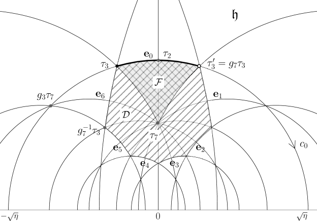
Figure 1: Fundamental domain

Remark 3.1.1.

In Figure 1, $g_{2}$ acts on $\mathfrak{h}$ as a rotation by $-\pi$ around $\tau_{2}$ (with respect to the hyperbolic metric on $\mathfrak{h}$), $g_{3}$ acts as a rotation by $-\frac{2\pi}{3}$ around $\tau_{3}$, and $g_{7}$ acts as a rotation by $-\frac{2\pi}{7}$ around $\tau_{7}$. These facts can be verified by using (3.65), (3.66), (3.67).

3.2 Geodesic continued fraction algorithm

Let $\varpi=\varpi_{\beta\to\alpha}$ be an oriented geodesic on $\mathfrak{h}$ joining $\beta$ to $\alpha$ ($\alpha,\beta\in\mathbb{R}\cup\{\infty\}$, $\alpha\neq\beta$). Note that if $\varpi\cap\mathcal{D}\neq\emptyset$, then there exist $P,Q\in\varpi$ such that $\varpi\cap\mathcal{D}=\overrightarrow{PQ}$ (possibly $P=Q$) because $\mathcal{D}$ is geodesically convex.

Definition 3.2.1.

1. We say that $\varpi$ enters (resp. leaves) $\mathcal{D}$ from $\mathbf{e}_{i}$ (resp. $\mathbf{e}_{i}^{\prime}$) if $\varpi\cap\mathcal{D}=\overrightarrow{PQ}$ for $P,Q\in\mathfrak{h}$ with $P\in\mathbf{e}_{i}$ (resp. $Q\in\mathbf{e}_{i}^{\prime}$).

2. We say that $\varpi$ is reduced if $\varpi$ enters $\mathcal{D}$ from $\mathbf{e}_{0}$ and $|\alpha|<\sqrt{\eta}$.

Remark 3.2.2.

1. The reduced oriented geodesics can be classified into three types according to the way they intersect with $\mathcal{D}$. See Figure 2 and Lemma 3.2.3.

2. The above definition of the reducedness of geodesics is an analogue of the reducedness of real quadratic irrationals or quadratic forms in the classical theory of continued fraction. See Remark 3.2.7.

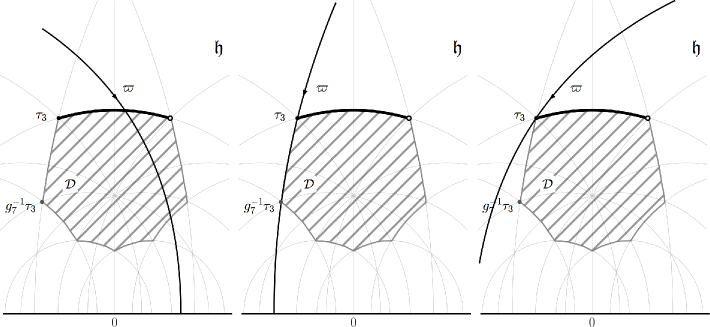
Figure 2: $3$ types of reduced geodesics

Lemma 3.2.3.

Let $\varpi=\varpi_{\beta\to\alpha}$ be an oriented geodesic on $\mathfrak{h}$ which enters $\mathcal{D}$ from $\mathbf{e}_{0}$ and leaves $\mathcal{D}$ from $\mathbf{e}_{i}^{\prime}$ $(i\in\mathbb{Z}/7\mathbb{Z})$. Then we have the following:

1. If $\varpi\cap\mathcal{D}^{\circ}\neq\emptyset$, then we have $i\neq 0$, and both $\varpi$ and $(g_{7}^{i}g_{2})^{-1}\varpi$ are reduced.

2. If $\varpi\cap\mathcal{D}=\overrightarrow{\tau_{3}(g_{7}^{-1}\tau_{3})}$, then we have $i=5$ and $\varpi=g_{3}c_{0}$. In particular, we see that both $\varpi$ and $(g_{7}^{5}g_{2})^{-1}\varpi$ are reduced, and that $(g_{7}^{5}g_{2})^{-1}\varpi\cap\mathcal{D}^{\circ}\neq\emptyset$.

3. If $\varpi\cap\mathcal{D}=\overrightarrow{\tau_{3}(g_{7}\tau_{3})}$, then we have $i=0$ and $\varpi=c_{0}$. In particular, we see that $\varpi$ is not reduced and $g_{3}\varpi$ is reduced.

4. If $\varpi\cap\mathcal{D}=\{\tau_{3}\}$, then we have $i=6$, and $(g_{7}^{6}g_{2})^{-1}\varpi\cap\mathcal{D}^{\circ}=g_{3}^{-1}\varpi\cap\mathcal{D}^{\circ}\neq\emptyset$. Moreover, in this case, $\varpi$ is reduced if and only if $(g_{7}^{6}g_{2})^{-1}\varpi$ is reduced.

As a result, for any reduced oriented geodesic $\varpi$, we see that there exists a unique index $i\in\mathbb{Z}/7\mathbb{Z}$, $i\neq 0$ such that $\varpi$ leaves $\mathcal{D}$ from $\mathbf{e}_{i}^{\prime}$. Moreover, for such $i$, $(g_{7}^{i}g_{2})^{-1}\varpi$ is again reduced.

Proof.

Suppose $\varpi\cap\mathcal{D}=\overrightarrow{PQ}$ wth $P\in\mathbf{e}_{0}$ and $Q\in\mathbf{e}_{i}^{\prime}$.

(1) First, if $i=0$, then we must have $P=\tau_{3}$, $Q=g_{7}\tau_{3}$, and hence $\varpi\cap\mathcal{D}^{\circ}=\emptyset$, which is a contradiction. Therefore, $i\neq 0$. Take $z\in\varpi\cap\mathcal{D}^{\circ}\subset S_{0}$. We have $P\in c_{0}$, $z\notin c_{0}$, and $z\in\bm{(}P,Q\bm{)}\subset\bm{(}P,\alpha\bm{)}$. If $|\alpha|\geq\sqrt{\eta}$, then we have either $\bm{(}P,\alpha\bm{)}\subset c_{0}$ or $\bm{(}P,\alpha\bm{)}\subset\mathfrak{h}-S_{0}$, which is a contradiction. Therefore, $\varpi$ is reduced. Next, set $\varpi^{\prime}:=(g_{7}^{i}g_{2})^{-1}\varpi$, $P^{\prime}:=(g_{7}^{i}g_{2})^{-1}P$, and $Q^{\prime}:=(g_{7}^{i}g_{2})^{-1}Q$. Then we see that $Q^{\prime}\in\varpi^{\prime}\cap\mathbf{e}_{0}$, $\bm{(}P^{\prime},Q^{\prime}\bm{)}\subset\mathfrak{h}-S_{0}$. These imply that $\varpi^{\prime}$ enters $\mathcal{D}$ from $\mathbf{e}_{0}$ and $|(g_{7}^{i}g_{2})^{-1}\alpha|<\sqrt{\eta}$, and hence $\varpi^{\prime}$ is reduced.

The assertions (2), (3) and the first half of (4) are clear. To see the latter half of (4), observe that (under the assumption $\varpi\cap\mathcal{D}=\{\tau_{3}\}$) $\varpi$ is reduced if and only if $-\sqrt{\eta}<\alpha<g_{3}\sqrt{\eta}$, where $g_{3}\sqrt{\eta}$ is the linear fractional transformation of $\sqrt{\eta}$ by $g_{3}$. Then we further see that this is equivalent to $(g_{7}^{6}g_{2})^{-1}\varpi$ being reduced.

The last assertion follows directly from (1) to (4). ∎

Lemma 3.2.4.

1. For any oriented geodesic $\varpi$ and $z\in\varpi$, there exists $\gamma\in\Delta(2,3,7)$ such that $\gamma\varpi$ is reduced and $\gamma z\in\mathcal{D}$.

2. For any oriented geodesic $\varpi$, there exists $\gamma\in\Delta(2,3,7)$ such that $\gamma\varpi$ is reduced and $\gamma\varpi\cap\mathcal{D}^{\circ}\neq\emptyset$.

3. Let $\varpi$ be a reduced oriented geodesic such that $\varpi\cap\mathcal{D}^{\circ}\neq\emptyset$ and let $z\in\varpi\cap\mathcal{D}^{\circ}$. Suppose $\gamma\varpi$ is reduced and $\gamma z\in\mathcal{D}$ for $\gamma\in\Delta(2,3,7)$. Then we have $\gamma=\pm 1$.

Proof.

(1) Since $\mathcal{F}\subset\mathcal{D}$, where $\mathcal{F}$ is the fundamental domain, there exists $\gamma^{\prime}\in\Delta(2,3,7)$ such that $\gamma^{\prime}z\in\gamma^{\prime}\varpi\cap\mathcal{D}=\overrightarrow{PQ}$ for some $P,Q\in\mathfrak{h}$. Suppose $P\in\mathbf{e}_{i}$, and set $\varpi^{\prime}:=g_{7}^{-i}\gamma^{\prime}\varpi$, $z^{\prime}:=g_{7}^{-i}\gamma^{\prime}z\in\mathcal{D}$. Then enters $\mathcal{D}$ from $\mathbf{e}_{0}$. If $\varpi^{\prime}\cap\mathcal{D}^{\circ}\neq\emptyset$ or $\varpi^{\prime}\cap\mathcal{D}=\overrightarrow{\tau_{3}(g_{7}^{-1}\tau_{3})}$, then by Lemma 3.2.3 (1), (2), $\varpi^{\prime}$ is reduced as desired. If $\varpi^{\prime}\cap\mathcal{D}=\overrightarrow{\tau_{3}(g_{7}\tau_{3})}$, then by Lemma 3.2.3 (3), we have $\varpi^{\prime}=c_{0}$, and hence we see that $g_{3}\varpi^{\prime}$ is reduced and $g_{3}z^{\prime}\in\mathcal{D}$. Otherwise, we have $\varpi^{\prime}\cap\mathcal{D}=\{\tau_{3}\}$ and $z^{\prime}=\tau_{3}$. In this case we easily see that either $\varpi^{\prime}$ is reduced or $g_{3}\varpi^{\prime}$ is reduced and $g_{3}z^{\prime}\in\mathcal{D}$.

(2) This follows from (1) and Lemma 3.2.3. Indeed, by (1), we can find $\gamma\in\Delta(2,3,7)$ such that $\gamma\varpi$ is reduced. Then by replacing $\gamma$ by $(g_{7}^{5}g_{2})^{-1}\gamma$ or $(g_{7}^{6}g_{2})^{-1}\gamma$ if necessary, we further obtain $\gamma\varpi\cap\mathcal{D}^{\circ}\neq\emptyset$.

(3) Suppose $\varpi\cap\mathcal{D}=\overrightarrow{PQ}$ and $\gamma z\in g_{7}^{i}\mathcal{F}$ ($i\in\mathbb{Z}/7\mathbb{Z}$). Then since $z\in\gamma^{-1}g_{7}^{i}\mathcal{F}\cap\mathcal{D}^{\circ}$, there exists $j\in\mathbb{Z}/7\mathbb{Z}$ such that $\gamma=\pm g_{7}^{j}$. In particular, we see that $\gamma\varpi\cap\mathcal{D}=\gamma\varpi\cap\gamma\mathcal{D}=\overrightarrow{\gamma P\gamma Q}$. On the other hand, since $\varpi$ and $\gamma\varpi$ are both reduced, we have $P\in\mathbf{e}_{0}$ and $\gamma P\in\mathbf{e}_{0}$. Therefore, we see that $j=0$, and hence $\gamma=\pm 1$. ∎

Now we define the geodesic continued fraction algorithm following the general principle of Morse [morse21], Series [series85], Katok [katok96]. Note that we slightly modify the original algorithm by using $\mathcal{D}$ instead of $\mathcal{F}$.

Definition 3.2.5 (Geodesic continued fraction algorithm for $\Delta(2,3,7)\backslash\mathfrak{h}$).

Let $\varpi$ be an oriented geodesic on $\mathfrak{h}$. Define $B_{0}\in\Delta(2,3,7)$ and $i_{k}\in\mathbb{Z}/7\mathbb{Z}\!-\!\{0\}$ ($k=1,2,3,\dots$) by the following algorithm:

• Find (any) $B_{0}\in\Delta(2,3,7)$ such that $B_{0}^{-1}\varpi$ is reduced, and set $\varpi_{0}:=B_{0}^{-1}\varpi$.

• For a given reduced oriented geodesic $\varpi_{k}$ ($k\geq 0$), find the unique $i_{k+1}\in\mathbb{Z}/7\mathbb{Z}\!-\!\{0\}$ such that $\varpi_{k}$ leaves $\mathcal{D}$ from $\mathbf{e}_{i_{k+1}}^{\prime}$. Set $\varpi_{k+1}:=(g_{7}^{i_{k+1}}g_{2})^{-1}\varpi_{k}$. Then by Lemma 3.2.3, $\varpi_{k+1}$ is again reduced.

We call this the geodesic continued fraction expansion of $\varpi$ (with respect to $\Delta(2,3,7)$), and express it as

$$\varpi=\llbracket B_{0};i_{1},i_{2},i_{3},\cdots\rrbracket_{\Delta(2,3,7)}\text{ or }B_{0}^{-1}\varpi=\llbracket i_{1},i_{2},i_{3},\cdots\rrbracket_{\Delta(2,3,7)}.$$ (3.2)

We review some basic properties of geodesic continued fraction expansion. See also Figure 4.

Proposition 3.2.6.

Let $\varpi$ be an oriented geodesic on $\mathfrak{h}$, and let

$$\varpi =\llbracket B_{0};i_{1},i_{2},i_{3},\cdots\rrbracket_{\Delta(2,3,7)}$$ (3.3)

be the geodesic continued fraction expansion of $\varpi$.

1. The choice of $B_{0}$ is not unique. However once we choose $B_{0}$, then the sequence $i_{1},i_{2},\dots$ are uniquely determined. More generally, let $\varpi^{\prime}$ be another oriented geodesic (possibly $\varpi^{\prime}=\varpi$), and let

   $$\varpi^{\prime}=\llbracket B_{0}^{\prime};j_{1},j_{2},j_{3},\cdots\rrbracket_{\Delta(2,3,7)},$$ (3.4)

   be the geodesic continued fraction expansion of $\varpi^{\prime}$ such that $(B_{0}^{\prime})^{-1}\varpi^{\prime}=B_{0}^{-1}\varpi$, then we have $j_{k}=i_{k}$ for all $k\geq 1$.

2. For $k\geq 1$, set $A_{k}:=g_{7}^{i_{k}}g_{2}\in\Delta(2,3,7)$ and $B_{k}:=B_{0}A_{1}A_{2}\cdots A_{k}\in\Delta(2,3,7)$ so that $\varpi_{k}=B_{k}^{-1}\varpi$ in the algorithm. Moreover define $P_{k},Q_{k}\in\varpi$ so that $\varpi\cap B_{k}\mathcal{D}=\overrightarrow{P_{k}Q_{k}}$. Then we have:

   1. $P_{k}\in B_{k}\mathbf{e}_{0}$, and $Q_{k}=P_{k+1}\in B_{k}\mathbf{e}_{i_{k+1}}^{\prime}$. In particular, we have $P_{k}\leq_{\varpi}P_{k+1}$.

   2. $P_{k}\neq Q_{k+1}=P_{k+2}$. In particular, we have $P_{k}<_{\varpi}P_{k+2}$.

   3. $B_{k}\mathcal{D}\neq B_{l}\mathcal{D}$ for $k\neq l$.

Proof.

(1) and (2) (i) are clear from Lemma 3.2.3, and Definition 3.2.5.

(2) (ii) Note that by (i) we have $P_{k}\leq_{\varpi}Q_{k}=P_{k+1}\leq_{\varpi}Q_{k+1}$ in general. Suppose $P_{k}=Q_{k+1}$. Then we have $P_{k}=Q_{k}=P_{k+1}=Q_{k+1}$, and hence $P_{k}=Q_{k}=B_{k}\tau_{3}$ and $P_{k+1}=Q_{k+1}=B_{k+1}\tau_{3}$. Therefore, it follows that $A_{k+1}=g_{7}^{-1}g_{2}=g_{3}$. Thus we get $B_{k}^{-1}\varpi\cap\mathcal{D}=g_{3}^{-1}B_{k}^{-1}\varpi\cap\mathcal{D}=\{\tau_{3}\}$, which is impossible by Lemma 3.2.3 (4).

(2) (iii) Suppose $B_{k}\mathcal{D}=B_{l}\mathcal{D}$ for $k\leq l$. Since $\mathcal{D}$ is geodesically convex, we have $P_{k}=P_{l}$ and $Q_{k}=Q_{l}$. Therefore, by (i) we obtain $P_{k}=P_{m}=Q_{m}=Q_{l}$ for all $k\leq m\leq l$. Then by (ii), we have $k=l$. ∎

Suppose that $\varpi$ joins $\beta$ to $\alpha$ ($\alpha,\beta\in\mathbb{R}\cup\{\infty\}$, $\alpha\neq\beta$), i.e., $\varpi=\varpi_{\beta\to\alpha}$. Suppose also that $\varpi$ is reduced for simplicity, and hence we take $B_{0}=1$ in the algorithm. Let

$$\varpi=\varpi_{\beta\to\alpha}=\llbracket i_{1},i_{2},i_{3},\dots\rrbracket_{\Delta(2,3,7)}$$ (3.5)

be the geodesic continued fraction expansion of $\varpi$. For $k\geq 1$, set $A_{k}:=g_{7}^{i_{k}}g_{2}\in\Delta(2,3,7)$ and $B_{k}:=A_{1}A_{2}\cdots A_{k}\in\Delta(2,3,7)$ as in Proposition 3.2.6. Then by the definition of the algorithm, the sequence $B_{k}\mathcal{D}$ ($k=1,2,3,\dots$) (of subsets of $\mathfrak{h}$) seems to “approach” to $\alpha$ as $k$ goes to $\infty$. See Figure 4. In fact we can prove

$$\alpha=\lim_{k\to\infty}B_{k}\tau_{7}.$$ (3.6)

See Theorem 3.3.2.

Now, note that for $\gamma=\begin{pmatrix}a&b\\ c&d\\ \end{pmatrix}\in SL_{2}(\mathbb{R})$ such that $c\neq 0$, we can rewrite the linear fractional transformation $\gamma z$ ($z\in\mathfrak{\mathbb{P}}^{1}(\mathbb{C})$) as

$$\gamma z=\frac{az+b}{cz+d}=\frac{a}{c}-\frac{1/c^{2}}{d/c+z}.$$ (3.7)

Therefore for $i\in\mathbb{Z}/7\mathbb{Z}\!-\!\{0\}$ we can define $\bm{a}_{i},\bm{b}_{i},\bm{c}_{i}\in L=\mathbb{Q}(\sqrt{\eta})$ by

$$g_{7}^{i}g_{2}z=:\bm{a}_{i}-\frac{\bm{b}_{i}}{\bm{c}_{i}+z}$$ (3.8)

because we easily see that the lower left component of $g_{7}^{i}g_{2}$ is non-zero for $i\neq 0$. In Section 3.5 we compute these constants $\bm{a}_{i},\bm{b}_{i},\bm{c}_{i}$ explicitly. Then we can formally rewrite (3.6) as

$$\alpha=\bm{a}_{i_{1}}-\cfrac{\bm{b}_{i_{1}}}{\bm{c}_{i_{1}}+\bm{a}_{i_{2}}-\cfrac{\bm{b}_{i_{2}}}{\bm{c}_{i_{2}}+\bm{a}_{i_{3}}-\cfrac{\bm{b}_{i_{3}}}{\bm{c}_{i_{3}}+\bm{a}_{i_{4}}-\cfrac{\bm{b}_{i_{4}}}{\bm{c}_{i_{4}}+\cdots}}}}$$ (3.9)

In the following section we study the convergence of this continued fraction expansion of $\alpha$.

Remark 3.2.7 (Remark on the case of $SL_{2}(\mathbb{Z})$).

Here we briefly explain the background of the above definitions of reducedness of a geodesic $\varpi$ and the geodesic continued fraction by comparing to the case of $SL_{2}(\mathbb{Z})$. Notations in this remark are independent of the rest of the paper.

As we have seen in Section 2.1, the modular curve $SL_{2}(\mathbb{Z})\backslash\mathfrak{h}$ is the Shimura curve associated to the quaternion algebra $M_{2}(\mathbb{Q})$ over $\mathbb{Q}$ and a maximal order $M_{2}(\mathbb{Z})$. Now, $SL_{2}(\mathbb{Z})$ is the $(2,3,\infty)$-triangle group $\Delta(2,3,\infty)$ generated by

$$g_{2}=\begin{pmatrix}0&-1\\ 1&0\\ \end{pmatrix},\quad g_{3}=\begin{pmatrix}-1&-1\\ 1&0\\ \end{pmatrix},\quad g_{\infty}=\begin{pmatrix}1&1\\ 0&1\\ \end{pmatrix}.$$ (3.10)

The triangle $\mathcal{F}=\left\{z\in\mathfrak{h}\mid|z|\geq 1,-\frac{1}{2}\leq\operatorname{Re}(z)\leq\frac{1}{2}\right\}$ is known to be a fundamental domain. Our regular geodesic heptagon corresponds to the $\infty$-gon $\mathcal{D}=\bigcup_{i\in\mathbb{Z}}g_{\infty}^{i}\mathcal{F}$, and our $\mathbf{e}_{i},\mathbf{e}_{i}^{\prime}$ correspond to

$$\mathbf{e}_{i} =\left\{z\in\mathfrak{h}~{}\left|~{}|z|=1,i-\frac{1}{2}<\operatorname{Re}(z)\leq i+\frac{1}{2}\right.\right\}$$ (3.11)

$$\mathbf{e}_{i}^{\prime} =\left\{z\in\mathfrak{h}~{}\left|~{}|z|=1,i-\frac{1}{2}\leq\operatorname{Re}(z)<i+\frac{1}{2}\right.\right\},$$ (3.12)

respectively. See Figure 3.

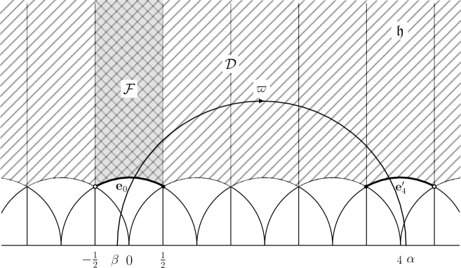
Figure 3: The case of $SL_{2}(\mathbb{Z})$

Let $\varpi=\varpi_{\beta\to\alpha}$ be the oriented geodesic on $\mathfrak{h}$ joining $\beta$ to $\alpha$ ($\alpha,\beta\in\mathbb{R}$). Then our definition of the reduced geodesics (Definition 3.2.1) in this case would be the following: $\varpi$ is said to be reduced if $\varpi$ enters $\mathcal{D}$ from $\mathbf{e}_{0}$ and $|\alpha|>1$. Then this condition can be seen roughly as:

$$|\beta|\text{``}<\text{''}1\text{ and }|\alpha|>1.$$ (3.13)

Hence we see that this definition is an analogue of the reducedness of real quadratic irrationals (cf. [zagier75]): a real quadratic irrational $\alpha$ is said to be reduced if $\alpha$ and its conjugate $\alpha^{\prime}$ (over $\mathbb{Q}$) satisfy

$$0<\alpha^{\prime}<1\text{ and }\alpha>1.$$ (3.14)

We also see that our geodesic continued fraction expansion of $\varpi$ in this case of $SL_{2}(\mathbb{Z})$ coincides with the one called the “geometric code” and studied in [katok96] by Katok. Furthermore since we have $g_{\infty}^{i}g_{2}z=i-\frac{1}{z},$ (3.9) becomes a variant of the so called “$-$”-continued fraction expansion.

3.3 Convergence

Perhaps the most traditional way to discuss the convergence of the above continued fraction (3.9) is to consider the limit of the following $k$-th convergent:

$$\bm{x}_{k}^{trad} =\bm{a}_{i_{1}}-\cfrac{\bm{b}_{i_{1}}}{\bm{c}_{i_{1}}+\bm{a}_{i_{2}}-\cfrac{\bm{b}_{i_{2}}}{\bm{c}_{i_{2}}+\cdots-\cfrac{\bm{b}_{i_{k}}}{\bm{c}_{i_{k}}+\bm{a}_{i_{k+1}}}}}$$ (3.15)

$$=B_{k}\bm{a}_{i_{k+1}}=B_{k+1}\infty,$$ (3.16)

Here $B_{k}\bm{a}_{i_{k+1}}$ and $B_{k+1}\infty$ are the linear fractional transformations of $\bm{a}_{i_{k+1}}$ and $\infty$. Unfortunately, however, we can give an example in which the traditional $k$-th convergent $\bm{x}_{k}^{trad}$ does not converge to $\alpha$. See Example 3.6.1.

Instead, we consider the following “regularized” $k$-th convergent:

$$\bm{x}^{reg}_{k}=B_{k}0=\bm{a}_{i_{1}}-\cfrac{\bm{b}_{i_{1}}}{\bm{c}_{i_{1}}+\bm{a}_{i_{2}}-\cfrac{\bm{b}_{i_{2}}}{\bm{c}_{i_{2}}+\cdots-\cfrac{\bm{b}_{i_{k}}}{\bm{c}_{i_{k}}}}},$$ (3.17)

which seems more natural in our setting since this $\bm{x}^{reg}_{k}$ corresponds to exactly the first $k$ steps of the geodesic continued fraction expansion of $\varpi$.

Definition 3.3.1.

Let $\bm{i}=(i_{k})_{k\geq 1}$ ($i_{k}\in\mathbb{Z}/7\mathbb{Z}\!-\!\{0\}$) be a sequence.

1. We define the associated formal continued fraction $\bm{x}(\bm{i})$ by the right hand side of (3.9)

2. We define the associated traditional $k$-th convergent $\bm{x}^{trad}_{k}(\bm{i})$ by the right hand side of (3.15). If the traditional $k$-th convergent $\bm{x}^{trad}_{k}(\bm{i})$ converges to $x\in\mathbb{P}^{1}(\mathbb{C})=\mathbb{C}\cup\{\infty\}$ with respect to the natural topology of $\mathbb{P}^{1}(\mathbb{C})$, we say that the continued fraction $\bm{x}(\bm{i})$ converges to $x$ in the traditional sense.

3. We define the associated regularized $k$-th convergent $\bm{x}^{reg}_{k}(\bm{i})$ by the right hand side of (3.17). If the regularized $k$-th convergent $\bm{x}^{reg}_{k}(\bm{i})$ converges to $x\in\mathbb{P}^{1}(\mathbb{C})=\mathbb{C}\cup\{\infty\}$ with respect to the natural topology of $\mathbb{P}^{1}(\mathbb{C})$, we say that the continued fraction $\bm{x}(\bm{i})$ converges to $x$ in the regularized sense.

Recall that $S_{0}=\{w\in\mathbb{C}\mid|w|\leq\sqrt{\eta},\ \operatorname{Im}(w)\geq 0\}\subset\overline{\mathfrak{h}}$ is the closed semicircle inside the geodesic $c_{0}$. We prove the following.

Theorem 3.3.2.

Let $\varpi=\varpi_{\beta\to\alpha}$ be an oriented geodesic on $\mathfrak{h}$ joining $\beta$ to $\alpha$, and let

$$B_{0}^{-1}\varpi=\llbracket i_{1},i_{2},i_{3},\cdots\rrbracket_{\Delta(2,3,7)}$$ (3.18)

be the geodesic continued fraction expansion of $\varpi$. For $k\geq 1$, set $A_{k}:=g_{7}^{i_{k}}g_{2}\in\Delta(2,3,7)$ and $B_{k}:=B_{0}A_{1}A_{2}\cdots A_{k}\in\Delta(2,3,7)$. We denote by $B_{k}S_{0}\subset\overline{\mathfrak{h}}$ the $B_{k}$-translation of $S_{0}$. Then for any sequence $(z_{k})_{k\geq 0}$ such that $z_{k}\in B_{k}S_{k}$, we have

$$\lim_{k\to\infty}z_{k}=\alpha$$ (3.19)

with respect to the natural topology of $\mathbb{P}^{1}(\mathbb{C})$. In particular, for any $z\in S_{0}$ we obtain

$$\lim_{k\to\infty}B_{k}z=\alpha.$$ (3.20)

Corollary 3.3.3.

The associated formal continued fraction $\bm{x}((i_{1},i_{2},\dots))$ converges to $B_{0}^{-1}\alpha$ in the regularized sense, i.e.,

$$\lim_{k\to\infty}\bm{x}^{reg}_{k}((i_{1},i_{2},\dots))=B_{0}^{-1}\alpha$$ (3.21)

Proof.

This follows from $0\in S_{0}$ and $B_{k}0=B_{0}A_{1}\cdots A_{k}0=B_{0}\bm{x}^{reg}_{k}((i_{1},i_{2},\dots))$. ∎

By the explicit computation of $\bm{a}_{i},\bm{b}_{i},\bm{c}_{i}$ in Section 3.5, we have $|\bm{a}_{1}|=|\bm{a}_{-1}|<|\bm{a}_{2}|=|\bm{a}_{-2}|<\sqrt{\eta}<|\bm{a}_{3}|=|\bm{a}_{-3}|$, cf. (3.74). From this and Theorem 3.3.2, we can also say a little bit about the convergence in the traditional sense.

Corollary 3.3.4.

We keep the notations in Theorem 3.3.2

1. Let $(k_{l})_{l\geq 1}$ be the subsequence of $(k)_{k\in\mathbb{Z}_{\geq 1}}$ consisting of those $k\geq 1$ such that $i_{k}\neq 3,4$ in $\mathbb{Z}/7\mathbb{Z}$. Then we have

   $$\lim_{l\to\infty}\bm{x}^{trad}_{k_{l}}((i_{1},i_{2},\dots))=B_{0}^{-1}\alpha.$$ (3.22)

2. In particular, if $i_{k}\neq 3,4$ in $\mathbb{Z}/7\mathbb{Z}$ for all sufficiently large $k\geq 1$, then the associated formal continued fraction $\bm{x}(\bm{i})$ converges to $B_{0}^{-1}\alpha$ in the traditional sense.

Proof of the convergence

Here we give a proof of Theorem 3.3.2.

Put $\Gamma:=\Delta(2,3,7)$ for simplicity. We may assume that $\varpi=\varpi_{\beta\to\alpha}$ is reduced and $B_{0}=1$. Recall that $c_{0}=\varpi_{-\sqrt{\eta}\to\sqrt{\eta}}$ is the oriented geodesic on $\mathfrak{h}$ which contains the edge $\mathbf{e}_{0}$. We denote by $u_{0}:=\sqrt{\eta}$, $v_{0}:=-\sqrt{\eta}$ the two endpoints of $c_{0}$. For $k\geq 0$ we define $c_{k}:=B_{k}c_{0}$, $u_{k}:=B_{k}u_{0}$, $v_{k}:=B_{k}v_{0}$, $S_{k}:=B_{k}S_{0}$ to be the $B_{k}$-translations of the corresponding objects. By the definition of the geodesic continued fraction algorithm, $B_{k}^{-1}\varpi$ is reduced. Thus we define $P_{k},Q_{k}\in\varpi$ ($k\geq 0$) so that $\varpi\cap B_{k}\mathcal{D}=\overrightarrow{P_{k}Q_{k}}$. Then by Proposition 3.2.6 (2) (i), we have $P_{k}\in\varpi\cap c_{k}$ and $Q_{k}=P_{k+1}\in\varpi\cap c_{k+1}$. See Figure 4.

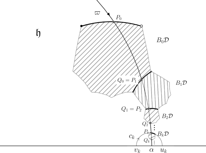
Figure 4: Geodesic continued fraction algorithm of $\varpi$

In the following we prepare six technical lemmas, most of which are intuitively clear. We adopt the usual notation of intervals in $\mathbb{P}^{1}(\mathbb{R})=\mathbb{R}\cup\{\infty\}$ by defining

$$(u,v)=\begin{cases}(u,v)&\text{ if }u,v\in\mathbb{R}\text{ and }u<v\\ (u,\infty)\cup\{\infty\}\cup(-\infty,v)&\text{ if }v,u\in\mathbb{R}\text{ and }v<u\\ (u,\infty)&\text{ if }u\in\mathbb{R},v=\infty\\ (-\infty,v)&\text{ if }v\in\mathbb{R},u=\infty,\end{cases}$$ (3.23)

for $u,v\in\mathbb{R}\cup\{\infty\}$ such that $u\neq v$.

Lemma 3.3.5.

For all $k\geq 0$ we have $\alpha\in(v_{k},u_{k})$ and $\beta\in(u_{k},v_{k})$.

Proof.

By the definition of the geodesic continued fraction algorithm, $B_{k}^{-1}\varpi$ is reduced, and hence we see $B_{k}^{-1}\alpha\in(v_{0},u_{0})$ and $B_{k}^{-1}\beta\in(u_{0},v_{0})$. Now the lemma follows from the fact that $SL_{2}(\mathbb{R})$ action preserves the intervals in $\mathbb{R}\cup\{\infty\}$, i.e., $g(u,v)=(gu,gv)$ for $g\in SL_{2}(\mathbb{R})$ and $u,v\in\mathbb{R}\cup\{\infty\}$ such that $u\neq v$. ∎

Next we observe the behavior of $c_{k}$ as $k$ goes to $\infty$, or more generally, the behavior of $\Gamma$-translations of $c_{0}$.

Lemma 3.3.6.

1. The projection $\overline{c_{0}}$ becomes a closed geodesic on $\Gamma\backslash\mathfrak{h}$, and there exists a hyperbolic element $\gamma_{0}\in\Gamma$ such that $\Gamma_{c_{0}}(=\{\gamma\in\Gamma\mid\gamma c_{0}=c_{0}\})=\{\pm\gamma_{0}^{k}\mid k\in\mathbb{Z}\}$.

2. In particular, we can decompose $c_{0}$ into a disjoint union of segments as

   $$c_{0}=\coprod_{k\in\mathbb{Z}}\gamma_{0}^{k}\bm{[}\tau_{3},\gamma_{0}\tau_{3}\bm{)}.$$ (3.24)

Proof.

(1) follows from Proposition 2.2.2 and Lemma 2.2.3 (5), (6). Indeed by choosing $z=w=1$, we obtain $D_{z,w}=(z-\bar{z})^{2}+4\eta w\bar{w}=4\eta$ and $\pm\sqrt{\eta}=\frac{1}{2w}((z-\bar{z})\pm\sqrt{D_{z,w}})$. (2) follows from (1) and $\tau_{3}\in c_{0}$. ∎

We consider the set

$$\mathbb{I}:=\{\gamma c_{0}\mid\gamma\in\Gamma,\#(\gamma c_{0}\cap c_{0})=1\}$$ (3.25)

of all $\Gamma$-translations of $c_{0}$ which intersect with $c_{0}$ at one point in $\mathfrak{h}$. Note that if two geodesics on $\mathfrak{h}$ has an intersection, then either they intersect at one point or they coincide up to the orientation.

Lemma 3.3.7.

There exist $c^{(1)},\dots,c^{(r)}\in\mathbb{I}$ (for some $r\geq 0$) such that

$$\mathbb{I}=\bigcup_{k\in\mathbb{Z}}\{\gamma_{0}^{k}c^{(1)},\dots,\gamma_{0}^{k}c^{(r)}\}.$$ (3.26)

If $\mathbb{I}=\emptyset$, then we assume $r=0$ and the both sides are the empty set.

Proof.

First, since $\Gamma=\Delta(2,3,7)$ acts properly discontinuously on $\mathfrak{h}$, we have

$$\#\{\gamma\in\Gamma\mid\#(\gamma\bm{[}\tau_{3},\gamma_{0}\tau_{3}\bm{]}\cap\bm{[}\tau_{3},\gamma_{0}\tau_{3}\bm{]})=1\}<\infty$$ (3.27)

Put $\{\gamma^{(1)},\dots\gamma^{(r)}\}:=\{\gamma\in\Gamma\mid\#(\gamma\bm{[}\tau_{3},\gamma_{0}\tau_{3}\bm{]}\cap\bm{[}\tau_{3},\gamma_{0}\tau_{3}\bm{]})=1\}$, and set $c^{(i)}:=\gamma^{(i)}c_{0}\in\mathbb{I}$ ($i=1,\dots,r$). Now, take any $\gamma c_{0}\in\mathbb{I}$. By Lemma 3.3.6 (2) there exists $k,l\in\mathbb{Z}$ such that

$$\#(\gamma\gamma_{0}^{l}\bm{[}\tau_{3},\gamma_{0}\tau_{3}\bm{)}\cap\gamma_{0}^{k}\bm{[}\tau_{3},\gamma_{0}\tau_{3}\bm{)})=1.$$ (3.28)

Then we get $\gamma=\gamma_{0}^{k}\gamma^{(i)}\gamma_{0}^{-l}$ for some $i\in\{1,\dots r\}$, and hence $\gamma c_{0}=\gamma_{0}^{k}c^{(i)}$. ∎

For $i=1,\dots,r$, we denote by $u^{(i)},v^{(i)}\in\mathbb{R}\cup\{\infty\}$ the two end points of $c^{(i)}$ such that $c^{(i)}=\varpi_{v^{(i)}\to u^{(i)}}$.

Lemma 3.3.8.

For any $\epsilon>0$ there exists $N>0$ such that for any $k\in\mathbb{Z}$, $i\in\{1,\dots,r\}$ and $z\in\gamma_{0}^{k}c^{(i)}$ with $|k|>N$, we have either $|z-u_{0}|<\epsilon$ or $|z-v_{0}|<\epsilon$.

Proof.

Now $\gamma_{0}$ is a hyperbolic element with fixed points $u_{0}$ and $v_{0}$. We may assume $u_{0}$ is the attracting point. On the other hand, we have $u^{(i)},v^{(i)}\notin\{u_{0},v_{0}\}$ because $\#(c^{(i)}\cap c_{0})=1$. Therefore we get $\lim_{k\to\infty}\gamma_{0}^{k}u^{(i)}=\lim_{k\to\infty}\gamma_{0}^{k}v^{(i)}=u_{0}$ and $\lim_{k\to-\infty}\gamma_{0}^{k}u^{(i)}=\lim_{k\to-\infty}\gamma_{0}^{k}v^{(i)}=v_{0}$. This proves the lemma. ∎

Lemma 3.3.9.

1. For $k\neq l$ we have $c_{k}\neq c_{l}$ as subsets of $\mathfrak{h}$.

2. For any fixed $l\geq 0$, we have $P_{k}\in S_{l}$ for all $k\geq l$.

3. For any fixed $k\geq 0$, we have $P_{k}\notin S_{l}$ for all $l\geq k+2$.

Proof.

(1) Suppose $c_{k}=c_{l}$ for $k\leq l$. Then we have $P_{k}=P_{l}$, and hence $l\leq k+2$ by Proposition 3.2.6 (2) (ii). On the other hand, by the definition of the algorithm, we easily see that $c_{k+1}\neq c_{k}$. Therefore, we obtain $k=l$.

(2), (3) These follow from Lemma 3.3.5 and Proposition 3.2.6 (2) (i), (ii). Indeed, since $S_{l}$ is geodeiscally convex and $\varpi\cap c_{l}=\{P_{l}\}$, we have $\bm{[}P_{l},\alpha\bm{)}=\varpi\cap S_{l}$ by Lemma 3.3.5. On the other hand we have $P_{k}\in\bm{[}P_{l},\alpha\bm{)}$ for $k\geq l$, and $P_{k}\notin\bm{[}P_{l},\alpha\bm{)}$ for $l\geq k+2$ by Proposition 3.2.6 (2) (i) and (ii) respectively. This proves the lemma. ∎

Lemma 3.3.10.

For any fixed $l\geq 0$ we have

$$\#\{k\geq 0\mid c_{k}\cap c_{l}\neq\emptyset\}<\infty.$$ (3.29)

Proof.

Suppose the contrary, i.e., there exists a subsequence $(k_{n})_{n\geq 1}$ of $(k)_{k\in\mathbb{Z}_{\geq 0}}$ such that $c_{k_{n}}\cap c_{l}\neq\emptyset$ for all $n\geq 1$. We may assume $k_{n}>l$ for all $n\geq 1$. Then we see $\#(c_{k_{n}}\cap c_{l})=1$ by Lemma 3.3.9 (1). Therefore we have $B_{l}^{-1}B_{k_{n}}c_{0}\in\mathbb{I}$ for all $n\geq 1$. By Lemma 3.3.7, for each $n$, the geodesic $B_{l}^{-1}B_{k_{n}}c_{0}$ can be written as $B_{l}^{-1}B_{k_{n}}c_{0}=\gamma_{0}^{m_{n}}c^{(i_{n})}$ for some $m_{n}\in\mathbb{Z}$ and $i_{n}\in\{1,\dots,r\}$. Moreover, since $B_{l}^{-1}B_{k_{n}}c_{0}$ ($n\geq 1$) are distinct by Lemma 3.3.9 (1), we see $|m_{n}|\to\infty$ as $n$ goes to $\infty$.

On the other hand, we have $B_{l}^{-1}P_{k_{n}}\in B_{l}^{-1}B_{k_{n}}c_{0}\cap B_{l}^{-1}\varpi$ for all $n\geq 1$. Therefore, by Lemma 3.3.8 and Lemma 3.3.9 (2), we obtain

$$B_{l}^{-1}\alpha=\lim_{n\to\infty}B_{l}^{-1}P_{k_{n}}\in\{u_{0},v_{0}\}.$$ (3.30)

However this contradicts to Lemma 3.3.5. ∎

Proof of Theorem 3.3.2.

By Lemma 3.3.10, there exists $l_{0}\geq 2$ such that for all $k\geq l_{0}$ we have $c_{k}\cap c_{0}=\emptyset$. Then for $k\geq l_{0}\geq 2$, we have either $S_{0}\subset S_{k}$ or $S_{k}\subset S_{0}$. However, by Lemma 3.3.9 (3) we have $P_{0}\notin S_{k}$, and hence $S_{0}\subset S_{k}$ can not happen, and we get $S_{k}\subsetneq S_{0}$ for all $k\geq l_{0}$. Then, inductively, we can find a strictly increasing sequence $(l_{n})_{n\geq 0}$ such that we have $S_{k}\subsetneq S_{l_{n-1}}$ for all $k\geq l_{n}$. Indeed, for given $l_{n-1}$, there exists $l_{n}\geq l_{n-1}+2$ such that $c_{k}\cap c_{l_{n-1}}=\emptyset$ for all $k\geq l_{n}$ by Lemma 3.3.10. Then we have $S_{k}\subsetneq S_{l_{n-1}}$ for all $k\geq l_{n}\geq l_{n-1}+2$ by Lemma 3.3.9 (3). In order to prove the theorem, it suffices to show

$$\bigcap_{n\geq 0}S_{l_{n}}=\{\alpha\}.$$ (3.31)

We denote by $S_{\infty}$ the left hand side of (3.31). Since $S_{k}$ are all closed semicircle, the intersection $S_{\infty}$ is also a closed semicircle, i.e., there exists $\xi\in\mathbb{R}(\cap S_{0})$ and $\lambda\geq 0$ such that $S_{\infty}=\{w\in\mathbb{C}\mid|w-\xi|\leq\lambda,\operatorname{Im}(w)\geq 0\}$. Suppose $\lambda>0$. Then $\xi+\sqrt{-1}\lambda\in\partial S_{\infty}$ is in $\mathfrak{h}$. Since $\mathcal{F}$ is a fundamental domain, $\{\gamma\in\Gamma\mid\xi+\sqrt{-1}\lambda\in\gamma\mathcal{F}\}$ is a non-empty finite set. Thus we set $\{\delta_{1},\dots,\delta_{m}\}:=\{\gamma\in\Gamma\mid\xi+\sqrt{-1}\lambda\in\gamma\mathcal{F}\}$, $V:=\bigcup_{j=1}^{m}\delta_{j}\mathcal{F}$, and put $U:=V^{\circ}$, where $V^{\circ}$ is the interior of $V$. Then $U$ is an open neighborhood of $\xi+\sqrt{-1}\lambda$, and thus there exists $N>0$ such that $U$ intersects with $c_{l_{n}}$ for all $n\geq N$. Therefore, there exists $j\in\{1,\dots,m\}$ such that $\delta_{j}\mathcal{F}$ intersects with $c_{l_{n}}=B_{l_{n}}c_{0}$ for infinitely many $n\geq N$. Now suppose $\delta_{j}\mathcal{F}$ intersects with $c_{l_{n}}=B_{l_{n}}c_{0}$. Then by Lemma 3.3.6 (2), there exists $k_{n}\in\mathbb{Z}$ such that $\gamma_{0}^{-k_{n}}B_{l_{n}}^{-1}\delta_{j}\mathcal{F}$ intersects with $\bm{[}\tau_{3},\gamma_{0}\tau_{3}\bm{)}$. Since $\Gamma$ acts properly discontinuously on $\mathfrak{h}$, there exist $n_{1}>n_{2}\geq N$ such that $\gamma_{0}^{-k_{n_{1}}}B_{l_{n_{1}}}^{-1}\delta_{j}\mathcal{F}=\gamma_{0}^{-k_{n_{2}}}B_{l_{n_{2}}}^{-1}\delta_{j}\mathcal{F}$. Thus $B_{n_{1}}=\pm B_{n_{2}}\gamma_{0}^{k_{n_{2}}-k_{n_{1}}}$, and hence $c_{n_{1}}=c_{n_{2}}$, which is a contradiction because $c_{k}$ are distinct by Lemma 3.3.9 (1). Therefore $\lambda=0$ and we obtain (3.31) by Lemma 3.3.5. ∎

3.4 Periodicity

Now we prove the Lagrange type periodicity theorem. We first prove the periodicity coming from the closed geodesics on $\Delta(2,3,7)\backslash\mathfrak{h}$, and then prove a refined “$\beta$-free” version by using the convergence of the geodesic continued fraction. As we have remarked in Section 1, the following Theorem 3.4.1 (1) follows directly from Proposition 2.2.2 and the well-known property of the geodesic continued fractions. However we have to discuss carefully in order to prove (2).

Theorem 3.4.1 (Lagrange’s theorem for $\Delta(2,3,7)\backslash\mathfrak{h}$).

1. Let $\alpha,\beta\in\mathbb{R}\cup\{\infty\}$ such that $\alpha\neq\beta$, and let $\varpi=\varpi_{\beta\to\alpha}$ be the oriented geodesic on $\mathfrak{h}$ joining $\beta$ to $\alpha$. Let

   $$B_{0}^{-1}\varpi=\llbracket i_{1},i_{2},i_{3},\cdots\rrbracket_{\Delta(2,3,7)}$$ (3.32)

   be the geodesic continued fraction expansion of $\varpi$ with respect to $\Delta(2,3,7)$. For $k\geq 1$, set $A_{k}:=g_{7}^{i_{k}}g_{2}\in\Delta(2,3,7)$, $B_{k}:=B_{0}A_{1}A_{2}\cdots A_{k}\in\Delta(2,3,7)$, and $\varpi_{k}:=B_{k}^{-1}\varpi$. Then the following conditions are equivalent.

   1. The two endpoints $\alpha$ and $\beta$ are of the following form:

      $$\begin{cases}\alpha&=\frac{1}{2w}(z-\bar{z}\pm\sqrt{D_{z,w}})\\ \beta&=\frac{1}{2w}(z-\bar{z}\mp\sqrt{D_{z,w}})\end{cases}$$ (3.33)

      for some $z,w\in L$ such that $D_{z,w}:=(z-\bar{z})^{2}+4\eta w\bar{w}>0$. Here if $w=0$, we assume $(\alpha,\beta)=(0,\infty)$ or $(\infty,0)$.

   2. There exists $l_{0}\geq 1$ such that $\varpi_{l_{0}}=\varpi_{0}$. (In particular the geodesic continued fraction expansion becomes periodic, i.e., $i_{k+l_{0}}=i_{k}$ for all $k\geq 1$.)

2. Suppose that the above conditions are satisfied for $z,w\in L$ and $l_{0}\geq 1$. Assume that $l_{0}$ is the minimal element such that the condition (ii) holds. Put $\gamma_{0}:=B_{l_{0}}B_{0}^{-1}=B_{0}A_{1}\cdots A_{l_{0}}B_{0}^{-1}$. Then we have $\gamma_{0}\in\Gamma_{\varpi}=\mathcal{O}_{z,w}^{1}$ (cf. Lemma 2.2.3 (5)), and $\gamma_{0}$ gives the fundamental unit of $\mathcal{O}_{z,w}^{1}$. Equivalently, $\rho_{\alpha}(\gamma_{0})\in F(\sqrt{D_{z,w}})$ gives the fundamental unit of $U_{\mathcal{O},z,w/F}$.

Proof.

(1) The implication (ii) $\Rightarrow$ (i) is clear from the implication (ii) $\Rightarrow$ (iii) of Proposition 2.2.2. Indeed (ii) implies $B_{l_{0}}B_{0}^{-1}\varpi=\varpi$, and we have $B_{0}\mathcal{D}\neq B_{l_{0}}\mathcal{D}$ by Proposition 3.2.6 (2) (iii). Therefore $B_{l_{0}}B_{0}^{-1}\neq\pm 1$ is a hyperbolic element in $\Gamma_{\varpi}$. We prove the implication (i) $\Rightarrow$ (ii). Since the conditions (i) and (ii) are preserved by replacing $\varpi$ with $\gamma\varpi$ for $\gamma\in\Delta(2,3,7)$ by Proposition 3.2.6 (1), we may assume $\varpi$ is reduced (i.e., $B_{0}=1$) and $\varpi\cap\mathcal{D}^{\circ}\neq\emptyset$ by Lemma 3.2.4 (2). We take $R\in\varpi\cap\mathcal{D}^{\circ}$, and define $P_{k},Q_{k}\in\varpi$ ($k\geq 0$) so that $\varpi\cap\mathcal{D}=\overrightarrow{P_{k}Q_{k}}$. By Proposition 2.2.2, there exists a hyperbolic element in $\Gamma_{\varpi}$. Let $\gamma_{0}\in\Gamma_{\varpi}$ be any hyperbolic element. By replacing $\gamma_{0}$ by $\gamma_{0}^{-1}$ if necessary we assume $\alpha$ is the attracting point of $\gamma_{0}$. Then we have $R\leq_{\varpi}\gamma_{0}R$. Furthermore, we have

$$P_{0}<_{\varpi}R<_{\varpi}Q_{0}=P_{1}<_{\varpi}\gamma_{0}R.$$ (3.34)

Indeed, if $\gamma_{0}R\in\mathcal{D}$, then by Lemma 3.2.4 (3), we obtain $\gamma_{0}=\pm 1$, which is a contradiction. On the other hand, by Proposition 3.2.6 and Theorem 3.3.2, we have $P_{k+1}=Q_{k}$ and $\lim_{k\to\infty}P_{k}=\lim_{k\to\infty}Q_{k}=\alpha$. Therefore, there exists $l_{0}\geq 1$ such that $\gamma_{0}R\in\bm{[}P_{l_{0}},Q_{l_{0}}\bm{)}$. Then we have $R\in\varpi\cap\mathcal{D}^{\circ}$ and $B_{l_{0}}^{-1}\gamma_{0}R\in B_{l_{0}}^{-1}\gamma_{0}\varpi\cap\mathcal{D}$ and $\varpi$ and $B_{l_{0}}^{-1}\gamma_{0}\varpi=B_{l_{0}}^{-1}\varpi$ are both reduced. Therefore by Lemma 3.2.4 (3), we obtain $B_{l_{0}}^{-1}\gamma_{0}=\pm 1$, and hence $\varpi_{l_{0}}=\gamma_{0}\varpi=\varpi_{0}$.

(2) We may assume $\varpi$ is reduced and $B_{0}=1$. Suppose $l_{0}$ is minimal. By the above argument, we see $B_{l_{0}}\in\Gamma_{\varpi}=\mathcal{O}_{z,w}^{1}$. On the other hand, let $\gamma_{0}$ be the hyperbolic element which generates of $\Gamma_{\varpi}$ up to $\pm 1$, and assume that $\alpha$ is the attracting point of $\gamma_{0}$. Then, again by the above argument, we obtain $\gamma_{0}=\pm B_{l_{0}^{\prime}}$ for some $l_{0}^{\prime}\geq 1$. Now by the periodicity (ii) and the minimality of $l_{0}$, we see $\gamma_{0}=B_{l_{0}^{\prime}}=B_{ml_{0}}=B_{l_{0}}^{m}$ for some $m\geq 1$. Then, since $\gamma_{0}$ generates $\Gamma_{\varpi}$, we obtain $m=1$. Therefore, we get $l_{0}^{\prime}=l_{0}$, and hence $B_{l_{0}}=\pm\gamma_{0}$ becomes the fundamental unit. This completes the proof. ∎

The $\beta$-free version

In order to discuss the refined version of the above theorem, we first prepare some lemmas. For $\alpha\in\mathbb{R}\cup\{\infty\}$, we denote by $\mathcal{G}_{\alpha}$ the set of oriented geodesics on $\mathfrak{h}$ which goes towards $\alpha$. We naturally identify $\mathcal{G}_{\alpha}$ with $\mathbb{P}^{1}(\mathbb{R})\!-\!\{\alpha\}=\mathbb{R}\cup\{\infty\}\!-\!\{\alpha\}$ as follows:

$$\mathbb{P}^{1}(\mathbb{R})\!-\!\{\alpha\}\overset{\sim}{\longrightarrow}\mathcal{G}_{\alpha};\beta\mapsto\varpi_{\beta\to\alpha}.$$ (3.35)

We equip $\mathcal{G}_{\alpha}$ with the natural topology of $\mathbb{P}^{1}(\mathbb{R})$ via this identification. Then for $w\in\mathfrak{h}$, we denote by $p_{\alpha}(w)\in\mathcal{G}_{\alpha}$ the unique oriented geodesic on $\mathfrak{h}$ which passes through $w$ and goes to $\alpha$. This defines a map

$$p_{\alpha}:\mathfrak{h}\rightarrow\mathcal{G}_{\alpha}$$ (3.36)

which is clearly continuous open map since $p_{\alpha}$ is a fiber bundle with fibers $\varpi_{\beta\to\alpha}$.

Now let $\varpi=\varpi_{\beta\to\alpha}$ be an oriented geodesic which satisfies the equivalent conditions of Proposition 2.2.2 and Theorem 3.4.1. Furthermore we assume that $\varpi$ is reduced and $\varpi\cap\mathcal{D}^{\circ}\neq\emptyset$. Take $R\in\varpi\cap\mathcal{D}^{\circ}$ and a hyperbolic element $\gamma_{0}\in\Gamma_{\varpi}$ which generates $\Gamma_{\varpi}$ up to $\pm 1$. We assume that $\alpha$ is the attracting point and $\beta$ is the repelling point of $\gamma_{0}$. Thus we have

$$\varpi=\coprod_{n\in\mathbb{Z}}\gamma_{0}^{n}\bm{[}R,\gamma_{0}R\bm{)}.$$ (3.37)

We regard $\varpi$ as an element in $\mathcal{G}_{\alpha}$. Then $\mathcal{G}_{\alpha}\!-\!\{\varpi\}$ has two connected components. We denote by

$$\mathcal{G}_{\alpha,\beta,+} :=\{\varpi_{\beta^{\prime}\to\alpha}\mid\beta^{\prime}\in(\beta,\alpha)\},$$ (3.38)

$$\mathcal{G}_{\alpha,\beta,-} :=\{\varpi_{\beta^{\prime}\to\alpha}\mid\beta^{\prime}\in(\alpha,\beta)\},$$ (3.39)

those two components. Here we use the notation (3.23). Let $S_{0}=\{w\in\mathbb{C}\mid|w|\leq\sqrt{\eta},\ \operatorname{Im}(z)\geq 0\}$ be as before.

Lemma 3.4.2.

Let $U\subset\mathcal{G}_{\alpha}$ be any connected open neighborhood of $\varpi$, then we have $\gamma_{0}^{-1}U\subset U$. In particular for all $\varpi^{\prime}\in U\!-\!\{\varpi\}$, we have $\gamma_{0}^{-1}\varpi^{\prime}\in U\!-\!\{\varpi\}$.

Proof.

This follows from the assumption that $\gamma_{0}$ is a hyperbolic element with attracting fixed point $\alpha$ and repelling fixed point $\beta$. ∎

Lemma 3.4.3.

There exists a connected open neighborhood $U\subset\mathcal{G}_{\alpha}$ of $\varpi$ such that for any $\varpi^{\prime}\in U\!-\!\{\varpi\}$ we have $\varpi^{\prime}\cap\mathcal{D}^{\circ}\neq\emptyset$ and

$$\varpi^{\prime}\cap S_{0}\cap\Delta(2,3,7)\tau_{3}=\emptyset,$$ (3.40)

i.e., for every $\varpi^{\prime}\in U\!-\!\{\varpi\}$, $\varpi^{\prime}$ intersects with $\mathcal{D}^{\circ}$ and does not contain $\Delta(2,3,7)$-translations of $\tau_{3}$ inside $S_{0}$.

Proof.

Since $\mathcal{D}$, $\gamma_{0}\mathcal{D}$, and $\bm{[}R,\gamma_{0}R\bm{]}$ are all compact, there exists a geodesically convex open set $V\subset\mathfrak{h}$ containing $\bm{[}R,\gamma_{0}R\bm{]}\cup\mathcal{D}\cup\gamma_{0}\mathcal{D}$ such that its closure $\overline{V}$ (in $\mathfrak{h}$) is compact. Then, since the action of $\Delta(2,3,7)$ on $\mathfrak{h}$ is properly discontinuous, we see $V\cap\Delta(2,3,7)\tau_{3}$ is a finite set. Thus we take $w_{1},\dots,w_{r}\in V$ such that

$$\{w_{1},\dots,w_{r}\}=V\cap\Delta(2,3,7)\tau_{3}.$$ (3.41)

Then $p_{\alpha}(V)\subset\mathcal{G}_{\alpha}$ becomes an open neighborhood of $\varpi$, and hence

$$U_{1}=p_{\alpha}(V)\!-\!\{p_{\alpha}(w_{1}),\dots,p_{\alpha}(w_{r})\}\cup\{\varpi\}$$ (3.42)

is also an open neighborhood of $\varpi$. Now since $\varpi$ enters $\mathcal{D}$ from $\mathbf{e}_{0}$ and $V$ is an open set containing $\mathcal{D}$, there exists $Q\in\varpi$ such that $Q\in V\!-\!S_{0}$. Thus we take an open neighborhood $W\subset V\!-\!S_{0}$ of $Q$ in $V\!-\!S_{0}$. Let $V_{0}\subset\mathcal{D}$ be an open neighborhood of $R$ in $\mathcal{D}$. We define an open subset $U$ of $\mathcal{G}_{\alpha}$ to be the connected component of

$$U_{1}\cap p_{\alpha}(V_{0})\cap p_{\alpha}(\gamma_{0}V_{0})\cap p_{\alpha}(W)\ni\varpi$$ (3.43)

containing $\varpi$. At this stage we know the following: for any $\varpi^{\prime}\in U\!-\!\{\varpi\}$, we have

$$\varpi^{\prime}\cap V\cap\Delta(2,3,7)\tau_{3}=\emptyset.$$ (3.44)

Therefore it remains to extend the $\Delta(2,3,7)\tau_{3}$-free region from $V$ to $S_{0}$. We prove the following:

Claim 1.

Let $\varpi^{\prime}\in U\!-\!\{\varpi\}$, then we have

$$\varpi^{\prime}\cap S_{0}\subset\bigcup_{n\geq 0}\gamma_{0}^{n}V.$$ (3.45)

Now, by Lemma 3.4.2, we have $\gamma_{0}^{-n}\varpi^{\prime}\in U\!-\!\{\varpi\}$ for all $n\geq 0$, and hence $\gamma_{0}^{-n}\varpi^{\prime}\in p_{\alpha}(V_{0})\cap p_{\alpha}(\gamma_{0}V_{0})$ for all $n\geq 0$. Therefore we see $\gamma_{0}^{-n}\varpi^{\prime}$ intersects with $V_{0}$ and $\gamma_{0}V_{0}$ for all $n\geq 0$, or equivalently, $\varpi^{\prime}$ intersects with $\gamma_{0}^{n}V_{0}$ and $\gamma_{0}^{n+1}V_{0}$ for all $n\geq 0$. On the other hand, by the definition, $\gamma_{0}^{n}V$ is a geodesically convex open set which contains $\gamma_{0}^{n}V_{0}$ and $\gamma_{0}^{n+1}V_{0}$. Therefore the geodesic segment of $\varpi^{\prime}$ between $\varpi^{\prime}\cap\gamma_{0}^{n}V_{0}$ and $\varpi^{\prime}\cap\gamma_{0}^{n+1}V_{0}$ is contained in $\gamma_{0}^{n}V$. Now, since $\alpha$ is the attracting point of $\gamma_{0}$, the points in $\gamma_{0}^{n}V$ converges to $\alpha$ uniformly as $n\to\infty$. Therefore the geodesic segment of $\varpi^{\prime}$ from $\varpi^{\prime}\cap V$ to $\alpha$ is contained in $\bigcup_{n\geq 0}\gamma_{0}^{n}V$. On the other hand since $W\subset V\!-\!S_{0}$ and $\varpi^{\prime}\in p_{\alpha}(W)$, we see that $\varpi^{\prime}\cap S_{0}$ is contained in the geodesic segment of $\varpi^{\prime}$ from $\varpi^{\prime}\cap V$ to $\alpha$. This proves the claim.

Now let $\varpi^{\prime}\in U\!-\!\{\varpi\}$ and let $P\in\varpi^{\prime}\cap S_{0}$. Then by Claim 1, there exists $n\geq 0$ such that $\gamma_{0}^{-n}P\in\gamma_{0}^{-n}\varpi^{\prime}\cap V$. On the other hand, we have $\gamma_{0}^{-n}\varpi^{\prime}\in U\!-\!\{\varpi\}$ by Lemma 3.4.2. Thus we get $\gamma_{0}^{-n}\varpi^{\prime}\cap V\cap\Delta(2,3,7)\tau_{3}=\emptyset$ by (3.44). Therefore $P\notin\Delta(2,3,7)\tau_{3}$. This proves the lemma. ∎

Let $U\subset\mathcal{G}_{\alpha}$ be a connected open neighborhood of $\varpi$ satisfying the condition in Lemma 3.4.3. Then $U\!-\!\{\varpi\}$ consists of two connected components

$$U_{+} =U\cap\mathcal{G}_{\alpha,\beta,+}$$ (3.46)

$$U_{-} =U\cap\mathcal{G}_{\alpha,\beta,-}.$$ (3.47)

Lemma 3.4.4.

Let $\varpi^{(1)},\varpi^{(2)}\in U_{+}$ (or $\varpi^{(1)},\varpi^{(2)}\in U_{-}$) be geodesics in the same connected component of $U\!-\!\{\varpi\}$. By the assumption, we can take $R_{1}\in\varpi^{(1)}\cap\mathcal{D}^{\circ}$ and $R_{2}\in\varpi^{(2)}\cap\mathcal{D}^{\circ}$. Let

$$\varpi^{(1)}=\llbracket B_{1,0};i_{1},i_{2},\dots\rrbracket_{\Delta(2,3,7)},$$ (3.48)

$$\varpi^{(2)}=\llbracket B_{2,0};j_{1},j_{2},\dots\rrbracket_{\Delta(2,3,7)}$$ (3.49)

be the geodesic continued fraction expansions of $\varpi^{(1)}$ and $\varpi^{(2)}$ such that $B_{1,0}^{-1}R_{1}\in\mathcal{D}^{\circ}$ and $B_{2,0}^{-1}R_{2}\in\mathcal{D}^{\circ}$. Then we have $B_{1,0}=\pm B_{2,0}$ and $i_{k}=j_{k}$ for all $k\geq 1$.

Proof.

We only prove the case $\varpi^{(1)},\varpi^{(2)}\in U_{+}$ since the case $\varpi^{(1)},\varpi^{(2)}\in U_{-}$ can be proved similarly. By Lemma 3.2.4 (3) and the definition of the algorithm, it suffices to show the following:

Claim 2.

Suppose $\gamma\in\Delta(2,3,7)$ satisfies $\gamma\mathcal{D}\cap\varpi^{(1)}\neq\emptyset$ and $\gamma\mathcal{D}\cap\varpi^{(2)}\neq\emptyset$ and $\gamma\mathcal{D}\subset S_{0}$. Then both $\gamma^{-1}\varpi^{(1)}$ and $\gamma^{-1}\varpi^{(2)}$ intersect with $\mathcal{D}^{\circ}$ and enter (resp. leave) $\mathcal{D}$ from the same edge, say $\mathbf{e}_{i}$ (resp. $\mathbf{e}_{j}^{\prime}$).

By Lemma 3.4.3, $\gamma\mathcal{D}\cap\varpi^{(1)}$ and $\gamma\mathcal{D}\cap\varpi^{(2)}$ do not contain vertices of $\gamma\mathcal{D}$. Therefore $\gamma^{-1}\varpi^{(1)}$ and $\gamma^{-1}\varpi^{(2)}$ must intersect with $\mathcal{D}^{\circ}$. Now let $I\subset U_{+}$ be the closed interval between $\varpi^{(1)}$ and $\varpi^{(2)}$ contained in $U_{+}$ (via the identification $\mathcal{G}_{\alpha}\simeq\mathbb{P}^{1}(\mathbb{R})\!-\!\{\alpha\}$). Then because $U$ satisfies the condition in Lemma 3.4.3, we have

$$p_{\alpha}^{-1}(I)\cap S_{0}\cap\Delta(2,3,7)\tau_{3}=\emptyset.$$ (3.50)

Suppose $\gamma^{-1}\varpi^{(1)}$ enters (resp. leaves) $\mathcal{D}$ from $\mathbf{e}_{i}$ (resp. $\mathbf{e}_{j}^{\prime}$). Now, since the endpoints $\gamma g_{7}^{i}\tau_{3}$ and $\gamma g_{7}^{i}\tau_{3}^{\prime}$ (resp. $\gamma g_{7}^{j}\tau_{3}$ and $\gamma g_{7}^{j}\tau_{3}^{\prime}$) of $\gamma\mathbf{e}_{i}$ (resp. $\gamma\mathbf{e}_{j}^{\prime}$) are contained in $S_{0}\cap\Delta(2,3,7)\tau_{3}$, they must not be contained in $p_{\alpha}^{-1}(I)$ by (3.50). On the other hand, the geodesic segment $\gamma\mathbf{e}_{i}$ (resp. $\gamma\mathbf{e}_{j}^{\prime}$) can intersect with $\varpi^{(1)}$ at most once. Therefore, $\gamma\mathbf{e}_{i}$ (resp. $\gamma\mathbf{e}_{j}^{\prime}$) must also intersect with $\varpi^{(2)}$. Finally, if $\gamma^{-1}\varpi^{(2)}$ leaves (resp. enters) $\mathcal{D}$ from $\mathbf{e}_{i}$ (resp. $\mathbf{e}_{j}^{\prime}$), this contradicts to the assumption that $\varpi^{(2)}$ is an oriented geodesic which goes to $\alpha$. This proves the claim and hence the lemma. ∎

Now we present the refined version of the above theorem in which we can get rid of the condition on $\beta$.

Theorem 3.4.5 (Lagrange’s theorem for $\Delta(2,3,7)\backslash\mathfrak{h}$, $\beta$-free version).

1. Let $\alpha,\beta\in\mathbb{R}\cup\{\infty\}$ such that $\alpha\neq\beta$, and let $\varpi=\varpi_{\beta\to\alpha}$ be the oriented geodesic on $\mathfrak{h}$ joining $\beta$ to $\alpha$. Let

   $$B_{0}^{-1}\varpi=\llbracket i_{1},i_{2},i_{3},\cdots\rrbracket_{\Delta(2,3,7)}$$ (3.51)

   be the geodesic continued fraction expansion of $\varpi$ with respect to $\Delta(2,3,7)$. For $k\geq 1$, set $A_{k}:=g_{7}^{i_{k}}g_{2}\in\Delta(2,3,7)$ and $B_{k}:=B_{0}A_{1}A_{2}\cdots A_{k}\in\Delta(2,3,7)$. Then the following conditions are equivalent.

   1. The endpoint $\alpha$ is of the following form:

      $$\alpha=\frac{1}{2w}(z-\bar{z}\pm\sqrt{D_{z,w}})$$ (3.52)

      for some $z,w\in L$ such that $D_{z,w}:=(z-\bar{z})^{2}+4\eta w\bar{w}>0$. Here when $w=0$, we assume $\alpha=\infty$ (resp. $0$) if the sign in $\alpha$ is $+$ (resp. $-$).

   2. There exist $l_{0}\geq 1$ and $k_{0}\geq 0$ such that $B_{k+l_{0}}^{-1}\alpha=B_{k}^{-1}\alpha$ for all $k\geq k_{0}$.

   3. There exist $l_{0}\geq 1$ and $k_{0}\geq 0$ such that $i_{k+l_{0}}=i_{k}$ for all $k>k_{0}$, i.e., the geodesic continued fraction expansion becomes periodic.

2. Suppose that the above conditions are satisfied for $z,w\in L$ and $l_{0},k_{0}\geq 1$. Assume that $l_{0}$ is the minimal element such that the condition (iii) holds. Put $\gamma_{0}:=B_{k_{0}+l_{0}}B_{k_{0}}^{-1}=B_{k_{0}}A_{k_{0}+1}\cdots A_{k_{0}+l_{0}}B_{k_{0}}^{-1}$. Then we have $\gamma_{0}\in\mathcal{O}_{z,w}^{1}$, and $\gamma_{0}$ gives the fundamental unit of $\mathcal{O}_{z,w}^{1}$. Equivalently, $\rho_{\alpha}(\gamma_{0})\in F(\sqrt{D_{z,w}})$ gives the fundamental unit of $U_{\mathcal{O},z,w/F}$.

Proof.

(1) The implication (ii) $\Rightarrow$ (i) is clear. The implication (iii) $\Rightarrow$ (ii) follows directly from the convergence of geodesic continued fraction (Corollary 3.3.3). We prove (i) $\Rightarrow$ (iii). Let $\beta^{\prime}:=\frac{z-\bar{z}}{w}-\alpha$, and let $\varpi^{\prime}:=\varpi_{\beta^{\prime}\to\alpha}$ be the oriented geodesic joining $\beta^{\prime}$ to $\alpha$. Here if $w=0$ and $\alpha=0$ (resp. $\alpha=\infty$), we assume $\beta^{\prime}=\infty$ (resp. $\beta^{\prime}=0$). We use this auxiliary geodesic $\varpi^{\prime}$ about which we have already studied in Theorem 3.4.1. In particular the case where $\beta=\beta^{\prime}$ is already proved in Theorem 3.4.1. Therefore we assume $\beta\neq\beta^{\prime}$. By Proposition 2.2.2, there exists a hyperbolic element in $\Gamma_{\varpi^{\prime}}$. Let $\delta_{0}\in\Gamma_{\varpi^{\prime}}$ be any hyperbolic element. We assume that $\alpha$ is the attracting point and $\beta^{\prime}$ is the repelling point of $\delta_{0}$. The key fact to prove this theorem is $\lim_{n\to\infty}\delta_{0}^{-n}\beta=\beta^{\prime}$.

By Lemma 3.2.4 (2) and Proposition 3.2.6 (1), we may assume $\varpi^{\prime}$ is reduced and $\varpi^{\prime}\cap\mathcal{D}^{\circ}\neq\emptyset$. Take $R^{\prime}\in\varpi^{\prime}\cap\mathcal{D}^{\circ}$. Then we can use Lemma 3.4.3 to take a connected open neighborhood $U\subset\mathcal{G}_{\alpha}$ of $\varpi^{\prime}$ such that for any $\varpi^{\prime\prime}\in U\!-\!\{\varpi^{\prime}\}$, we have $\varpi^{\prime\prime}\cap\mathcal{D}^{\circ}\neq\emptyset$, and

$$\varpi^{\prime\prime}\cap S_{0}\cap\Delta(2,3,7)\tau_{3}=\emptyset.$$ (3.53)

We denote by $U_{+},U_{-}$ the connected components of $U\!-\!\{\varpi^{\prime}\}$ as in (3.46), (3.47). Since we have assumed that $\beta\neq\beta^{\prime}$, we have $\varpi\in\mathcal{G}_{\alpha}\!-\!\{\varpi^{\prime}\}=\mathcal{G}_{\alpha,\beta^{\prime},+}\cup\mathcal{G}_{\alpha,\beta^{\prime},-}$. Suppose $\varpi\in\mathcal{G}_{\alpha,\beta^{\prime},+}$ (resp. $\mathcal{G}_{\alpha,\beta^{\prime},-}$). Then, since we have $\lim_{n\to\infty}\delta_{0}^{-n}\beta=\beta^{\prime}$ and $\delta_{0}\mathcal{G}_{\alpha,\beta^{\prime},+}=\mathcal{G}_{\alpha,\beta^{\prime},+}$ (resp. $\delta_{0}\mathcal{G}_{\alpha,\beta^{\prime},-}=\mathcal{G}_{\alpha,\beta^{\prime},-}$), there exists $N_{1}\geq 0$ such that $\delta_{0}^{-n}\varpi\in U_{+}$ (resp. $U_{-}$) for all $n\geq N_{1}$. Take $R_{n}\in\delta_{0}^{-n}\varpi\cap\mathcal{D}^{\circ}$ for each $n\geq N_{1}$. Since $\alpha$ is the attracting point of $\delta_{0}$, we have $\lim_{n\to\infty}\delta_{0}^{n}R_{n}=\alpha$.

Now, as in the proof of Theorem 3.4.1, we define $P_{k},Q_{k}\in\varpi$ ($k\geq 0$) so that $\varpi\cap B_{k}\mathcal{D}=\overrightarrow{P_{k}Q_{k}}$. Let us fix a constant $M\in\mathbb{Z}_{\geq 0}$ arbitrarily. (We use this later.) By Proposition 3.2.6 and Theorem 3.3.2, we have $P_{k+1}=Q_{k}$ and $\lim_{k\to\infty}P_{k}=\lim_{k\to\infty}Q_{k}=\alpha$. Therefore, there exist $N_{2}\geq N_{1}$, $k_{0}\geq M$, and $l_{0}\geq 1$ such that

$$\delta_{0}^{N_{2}}R_{N_{2}} \in\bm{[}P_{k_{0}},Q_{k_{0}}\bm{)}\subset\varpi,$$ (3.54)

$$\delta_{0}^{N_{2}+1}R_{N_{2}+1} \in\bm{[}P_{k_{0}+l_{0}},Q_{k_{0}+l_{0}}\bm{)}\subset\varpi.$$ (3.55)

Let

$$C_{0}^{-1}(\delta_{0}^{-N_{2}}\varpi) =\llbracket j_{1},j_{2},\dots\rrbracket_{\Delta(2,3,7)}$$ (3.56)

$$(C_{0}^{\prime})^{-1}(\delta_{0}^{-N_{2}-1}\varpi) =\llbracket j_{1}^{\prime},j_{2}^{\prime},\dots\rrbracket_{\Delta(2,3,7)}$$ (3.57)

be the geodesic continued fraction expansions of $\delta_{0}^{-N_{2}}\varpi$ and $\delta_{0}^{-N_{2}-1}\varpi$ such that

$$C_{0}^{-1}R_{N_{2}}\in\mathcal{D}^{\circ}\quad\text{ and }\quad(C_{0}^{\prime})^{-1}R_{N_{2}+1}\in\mathcal{D}^{\circ}.$$ (3.58)

Then, by Lemma 3.4.4, we have $C_{0}=\pm C_{0}^{\prime}$ and $j_{k}=j_{k}^{\prime}$ for all $k\geq 1$. On the other hand, from the geodesic continued fraction expansion (3.51), we also obtain the following geodesic continued fraction expansions:

$$B_{k_{0}}^{-1}\varpi =\llbracket i_{k_{0}+1},i_{k_{0}+2},\dots\rrbracket_{\Delta(2,3,7)},$$ (3.59)

$$B_{k_{0}+l_{0}}^{-1}\varpi =\llbracket i_{k_{0}+l_{0}+1},i_{k_{0}+l_{0}+2},\dots\rrbracket_{\Delta(2,3,7)},$$ (3.60)

Now we apply Lemma 3.2.4 (3) to

• the reduced oriented geodesic: $C_{0}^{-1}(\delta_{0}^{-N_{2}}\varpi)$ (resp. $(C_{0}^{\prime})^{-1}(\delta_{0}^{-N_{2}-1}\varpi)$),

• point: $z=C_{0}^{-1}R_{N_{2}}\in\mathcal{D}^{\circ}$, (resp. $z=(C_{0}^{\prime})^{-1}R_{N_{2}+1}\in\mathcal{D}^{\circ}$),

• $\gamma=B_{k_{0}}^{-1}\delta_{0}^{N_{2}}C_{0}\in\Delta(2,3,7)$, (resp. $\gamma=B_{k_{0}+l_{0}}^{-1}\delta_{0}^{N_{2}+1}C_{0}^{\prime}\in\Delta(2,3,7)$).

Because we have

• $\gamma C_{0}^{-1}(\delta_{0}^{-N_{2}}\varpi)=B_{k_{0}}^{-1}\varpi$ (resp. $\gamma(C_{0}^{\prime})^{-1}(\delta_{0}^{-N_{2}-1}\varpi)=B_{k_{0}+l_{0}}^{-1}\varpi$) is reduced by the definition of the geodesic continued fraction expansion,

• $\gamma z=B_{k_{0}}^{-1}\delta_{0}^{N_{2}}R_{N_{2}}\in\mathcal{D}$ (resp. $\gamma z=B_{k_{0}+l_{0}}^{-1}\delta_{0}^{N_{2}+1}R_{N_{2}+1}\in\mathcal{D}$) by (3.54) (resp. (3.55)),

we obtain

$$B_{k_{0}}^{-1}\delta_{0}^{N_{2}}C_{0}=\pm 1\quad\text{ and }\quad B_{k_{0}+l_{0}}^{-1}\delta_{0}^{N_{2}+1}C_{0}^{\prime}=\pm 1.$$ (3.61)

Then it follows that both (3.56) and (3.59) give the geodesic continued fraction expansion of $C_{0}^{-1}\delta_{0}^{-N_{2}}\varpi=B_{k_{0}}^{-1}\varpi$, and both (3.57) and (3.60) give the geodesic continued fraction expansion of $(C_{0}^{\prime})^{-1}\delta_{0}^{-N_{2}-1}\varpi=B_{k_{0}+l_{0}}^{-1}\varpi$. Therefore, by using Proposition 3.2.6 (1), we finally obtain

$$i_{k_{0}+k}=j_{k}=j^{\prime}_{k}=i_{k_{0}+l_{0}+k}$$ (3.62)

for all $k\geq 1$. Thus we obtain (iii).

(2) We may assume $\beta\neq\beta^{\prime}$, $\varpi^{\prime}$ is reduced and $\varpi\cap\mathcal{D}^{\circ}\neq\emptyset$, where $\beta^{\prime}$ and $\varpi^{\prime}$ are the same objects as in the proof of the implication (i) $\Rightarrow$ (iii). Suppose that the equivalent conditions (i) $\sim$ (iii) are satisfied. More precisely, suppose that the condition (iii) is satisfied for $k_{0},l_{0}$, and that $l_{0}$ is the minimal element such that the condition (iii) holds. Then clearly the condition (ii) is also satisfied for the same $k_{0}$ and $l_{0}$. By the condition (ii), we have $B_{k_{0}+l_{0}}B_{k_{0}}^{-1}\alpha=\alpha$. Therefore, by Lemma 2.2.3 (5), we obtain $\gamma_{0}:=B_{k_{0}+l_{0}}B_{k_{0}}^{-1}\in K_{z,w}\cap\mathcal{O}^{1}=\mathcal{O}_{z,w}^{1}=\Gamma_{\varpi^{\prime}}$. On the other hand, let $\delta_{0}$ be the hyperbolic element which generates $\Gamma_{\varpi^{\prime}}=\mathcal{O}_{z,w}^{1}$ up to $\pm 1$, and assume that $\alpha$ is the attracting point of $\delta_{0}$. Then, by the above argument, especially from (3.61) and (3.62), there exist $k_{0}^{\prime}\geq k_{0}$ and $l_{0}^{\prime}\geq 1$ such that $i_{k+l_{0}^{\prime}}=i_{k}$ for all $k>k_{0}^{\prime}$ and $\delta_{0}=\pm B_{k_{0}^{\prime}+l_{0}^{\prime}}B_{k_{0}^{\prime}}^{-1}$. (Here we choose $M=k_{0}$ in the above argument.) Now, by the periodicity (iii), we have $A_{k+l_{0}}=A_{k}$ for all $k\geq k_{0}$. Therefore we have $\gamma_{0}=B_{k_{0}+l_{0}}B_{k_{0}}^{-1}=B_{k_{0}^{\prime}+l_{0}}B_{k_{0}^{\prime}}^{-1}$ by the definition of $B_{k}$. Thus, again by the periodicity (iii) and the minimality of $l_{0}$, we obtain

$$\delta_{0}=\pm B_{k_{0}^{\prime}+l_{0}^{\prime}}B_{k_{0}^{\prime}}^{-1}=B_{k_{0}^{\prime}+ml_{0}}B_{k_{0}^{\prime}}^{-1}=(B_{k_{0}^{\prime}+l_{0}}B_{k_{0}^{\prime}}^{-1})^{m}=\gamma_{0}^{m}$$ (3.63)

for some $m\geq 1$. Then, since $\delta_{0}$ generates $\Gamma_{\varpi^{\prime}}$, we obtain $m=1$. Therefore, we get $l_{0}^{\prime}=l_{0}$, and hence $\gamma_{0}=B_{k_{0}+l_{0}}B_{k_{0}}^{-1}=\pm\delta_{0}$ becomes the fundamental unit. This completes the proof. ∎

Remark 3.4.6.

The results in [series86] and [abramskatok19] are interesting, and seem to be related to the “$\beta$-free” version of the periodicity. Although their results do not cover the case of the $(2,3,7)$-triangle group, they compare the geodesic continued fractions (Morse codings) and the “boundary expansions” of geodesics which essentially depends only on the one end point $\alpha$. It may be possible to prove (1) of Theorem 3.4.5 using the similar arguments to those in [series86] and [abramskatok19]. Our proof is different from their methods.

3.5 Some explicit constants

Here we present some explicit computation of the elements such as $g_{2},g_{3},g_{7}$, $\bm{a}_{i},\bm{b}_{i},\bm{c}_{i}$ ($i\in\mathbb{Z}/7\mathbb{Z}\!-\!\{0\}$).

Recall that $A$ is the quaternion algebra $\left(\dfrac{\eta,\eta}{F}\right)=F+Fi+Fj+Fk$ over $F=\mathbb{Q}(\eta)$, where $i,j,k$ satisfy $i^{2}=j^{2}=\eta$ and $ij=-ji=k$, and $L=\mathbb{Q}(\sqrt{\eta})\subset\mathbb{R}$ is the fixed splitting field of $A$. We have embedded $A$ into $M_{2}(\mathbb{R})$ as

$$\iota:A\overset{\sim}{\rightarrow}\left\{\left.\begin{pmatrix}z&\eta\bar{w}\\ w&\bar{z}\end{pmatrix}\right|z,w\in L\right\}\subset M_{2}(\mathbb{R});\begin{cases}i&\mapsto\begin{pmatrix}0&\eta\\ 1&0\\ \end{pmatrix}\vspace{1mm}\\ j&\mapsto\begin{pmatrix}\sqrt{\eta}&0\\ 0&-\sqrt{\eta}\\ \end{pmatrix}\end{cases}.$$ (3.64)

Then the elements $g_{2},g_{3},g_{7}\in\Delta(2,3,7)\subset SL_{2}(\mathbb{R})$ (cf. (2.25), (2.26), (2.27)) are of the following form:

$$g_{2} =\begin{pmatrix}0&-\sqrt{\eta}\\ 1/\sqrt{\eta}&0\\ \end{pmatrix},$$ (3.65)

$$g_{3} =\frac{1}{2}\begin{pmatrix}1+(\eta^{2}-2)\sqrt{\eta}&-(\eta^{2}+\eta-1)\sqrt{\eta}\\ (3-\eta^{2})\sqrt{\eta}&1-(\eta^{2}-2)\sqrt{\eta}\\ \end{pmatrix},$$ (3.66)

$$g_{7} =\frac{1}{2}\begin{pmatrix}\eta^{2}+\eta-1&\eta^{2}-1-\sqrt{\eta}\\ 2-\eta^{2}+(\eta^{2}+\eta-2)\sqrt{\eta}&\eta^{2}+\eta-1\\ \end{pmatrix}.$$ (3.67)

Put $\theta=\sqrt{\eta}$ for simplicity. Then we can compute $\bm{a}_{i},\bm{b}_{i},\bm{c}_{i}$ ($i\in\mathbb{Z}/7\mathbb{Z}\!-\!\{0\}$) as follows:

$$\left\{\begin{aligned} \bm{a}_{1}&=-\bm{a}_{-1}&&=\theta-\theta^{2}+\theta^{4}-\theta^{5}\quad\quad\quad~{}&&=-\eta+\eta^{2}+(1-\eta^{2})\sqrt{\eta}\quad\quad~{}\\ \bm{b}_{1}&=\bm{b}_{-1}&&=4+8\theta^{2}-8\theta^{4}&&=4(1+2\eta-2\eta^{2})\\ \bm{c}_{1}&=-\bm{c}_{-1}&&=\theta+\theta^{2}-\theta^{4}-\theta^{5}&&=\eta-\eta^{2}+(1-\eta^{2})\sqrt{\eta}\end{aligned}\right.$$ (3.68)

$$\left\{\begin{aligned} \bm{a}_{2}&=-\bm{a}_{-2}&&=-2-3\theta+\theta^{2}+\theta^{4}+\theta^{5}~{}&&=-2+\eta+\eta^{2}+(-3+\eta^{2})\sqrt{\eta}\\ \bm{b}_{2}&=\bm{b}_{-2}&&=-8+4\theta^{2}+4\theta^{4}&&=4(-2+\eta+\eta^{2})\\ \bm{c}_{2}&=-\bm{c}_{-2}&&=2-3\theta-\theta^{2}-\theta^{4}+\theta^{5}&&=2-\eta-\eta^{2}+(-3+\eta^{2})\sqrt{\eta}\end{aligned}\right.$$ (3.69)

$$\left\{\begin{aligned} \bm{a}_{3}&=-\bm{a}_{-3}&&=-\theta+\theta^{2}-2\theta^{3}+\theta^{4}-\theta^{5}&&=\eta+\eta^{2}-(1+2\eta+\eta^{2})\sqrt{\eta}\\ \bm{b}_{3}&=\bm{b}_{-3}&&=4+12\theta^{2}+4\theta^{4}&&=4(1+3\eta+\eta^{2})\\ \bm{c}_{3}&=-\bm{c}_{-3}&&=-\theta-\theta^{2}-2\theta^{3}-\theta^{4}-\theta^{5}&&=-\eta-\eta^{2}-(1+2\eta+\eta^{2})\sqrt{\eta}.\end{aligned}\right.$$ (3.70)

We can also easily check the following properties of these constants. For $j\in\mathbb{Z}/7\mathbb{Z}\!-\!\{0\}$,

$$\bm{a}_{j} =g_{7}^{j}~{}0=(g_{7}^{j}g_{2})\infty\in\mathcal{O}_{L},$$ (3.71)

$$-\bm{c}_{j} =\overline{\bm{a}_{j}}=(g_{7}^{j}g_{2})^{-1}\infty\in\mathcal{O}_{L},$$ (3.72)

$$\bm{b}_{j}/4 =\frac{\eta}{\left(2\cos\left(\frac{j\pi}{7}\right)\right)^{2}}=\frac{2\cos\left(\frac{2\pi}{7}\right)}{\left(2\cos\left(\frac{j\pi}{7}\right)\right)^{2}}\in\mathcal{O}_{F}^{\times},$$ (3.73)

$$|\bm{a}_{1}| =|\bm{a}_{-1}|<|\bm{a}_{2}|=|\bm{a}_{-2}|<\sqrt{\eta}<|\bm{a}_{3}|=|\bm{a}_{-3}|.$$ (3.74)

3.6 Examples

Now we present some examples to illustrate our main theorems (Theorem 3.4.1 and Theorem 3.4.5). We describe the following items:

1. Input data: $(\alpha,\beta,\varpi_{\beta\to\alpha})$, where $\alpha,\beta\in\mathbb{R}\cup\{\infty\}$ such that $\alpha\neq\beta$ and $\varpi_{\beta\to\alpha}$ is the oriented geodesic joining $\beta$ to $\alpha$ as before.

2. The resulting geodesic continued fraction expansion of $\varpi_{\beta\to\alpha}$.

Suppose the geodesic continued fraction expansion of $\varpi_{\beta\to\alpha}$ becomes periodic (which is the case we are mainly interested in). As in the classical theory of continued fraction, we denote by

$$\varpi_{\beta\to\alpha}=\llbracket B_{0};i_{1},\dots,i_{k_{0}},\overline{i_{k_{0}+1},\dots,i_{k_{0}+l_{0}}}\rrbracket_{\Delta(2,3,7)},$$ (3.75)

the periodic geodesic continued fraction expansion with period $i_{k_{0}+1},\dots,i_{k_{0}+l_{0}}$. Then, furthermore we present

1. The data $z,w\in L$ for which $\alpha$ can be expressed as in Theorem 3.4.5 (i), and the associated quadratic extension $K_{z,w}\simeq F(\sqrt{D_{z,w}})$ over $F$.

2. The fundamental unit of $\mathcal{O}_{z,w}^{1}\simeq U_{\mathcal{O},z,w/F}$ obtained from the period of geodesic continued fraction expansion. Cf. Theorem 3.4.1 and Theorem 3.4.5.

We put $\theta:=\sqrt{\eta}$ as before. Moreover, for the geodesic continued fraction expansion (3.2) of $\varpi$, we put $A_{k}:=g_{7}^{i_{k}}g_{2}$, $B_{k}:=B_{0}A_{1}\cdots A_{k}$ and $\varpi_{k}:=B_{k}^{-1}\varpi$.

Example 3.6.1.

1. Input: $\alpha=0$, $\beta=\infty$, $\varpi:=\varpi_{\beta\to\alpha}$.

2. The corresponding data: $z=\sqrt{\eta}$, $w=0$, $D_{z,w}=4\eta$.
   The associated quadratic extension: $K_{z,w}\simeq F(\sqrt{\eta})=L$.

3. The geodesic continued fraction expansion:

   $$\varpi=\llbracket 1;\overline{3,-2,3}\rrbracket_{\Delta(2,3,7)}.$$ (3.76)

4. From the period, we obtain the following fundamental unit $\gamma_{0}$, i.e., a generator of $\mathcal{O}_{z,w}^{1}=\Gamma_{\varpi_{\beta\to\alpha}}$ up to $\pm 1$:

   $$\gamma_{0} :=B_{3}B_{0}^{-1}=(g_{7}^{3}g_{2})(g_{7}^{-2}g_{2})(g_{7}^{3}g_{2})$$ (3.77)

   $$=\begin{pmatrix}-1-\theta-\theta^{2}+\theta^{3}+\theta^{5}&0\\ 0&-1+\theta-\theta^{2}-\theta^{3}-\theta^{5}\\ \end{pmatrix}$$ (3.78)

   $$=\begin{pmatrix}-1-\eta-(1-\eta-\eta^{2})\sqrt{\eta}&0\\ 0&-1-\eta+(1-\eta-\eta^{2})\sqrt{\eta}\\ \end{pmatrix}.$$ (3.79)

   Under the identification (2.18), the fundamental unit $\varepsilon_{0}=\rho_{\alpha}(\gamma_{0})$ of $U_{\mathcal{O},z,w/F}$ can be written as

   $$\varepsilon_{0}=-1-\eta+(1-\eta-\eta^{2})\sqrt{\eta}\in U_{\mathcal{O},z,w/F}.$$ (3.80)

This example gives an example in which the traditional $k$-th convergent $\bm{x}^{trad}_{k}$ does not converges to $\alpha=0$. Indeed, by (3.16), we see

$$\bm{x}^{trad}_{3k-1}=((g_{7}^{3}g_{2})(g_{7}^{-2}g_{2})(g_{7}^{3}g_{2}))^{k}\infty=\infty\nrightarrow 0.$$ (3.81)

Example 3.6.2.

1. Input: $\alpha=(1-\eta^{2})\sqrt{\eta}+\sqrt{1+3\eta-2\eta^{2}}$, $\beta=(1-\eta^{2})\sqrt{\eta}-\sqrt{1+3\eta-2\eta^{2}}$, $\varpi:=\varpi_{\beta\to\alpha}$.

2. The corresponding data: $z=(1-\eta^{2})\sqrt{\eta}$, $w=1$, $D_{z,w}=4(1+3\eta-2\eta^{2})$.
   The associated quadratic extension: $K_{z,w}\simeq F(\sqrt{1+3\eta-2\eta^{2}})$.

3. The geodesic continued fraction expansion:

   $$\varpi=\llbracket 1;\overline{1,-1}\rrbracket_{\Delta(2,3,7)}.$$ (3.82)

4. From the period, we obtain the following fundamental unit $\gamma_{0}$, i.e., a generator of $\mathcal{O}_{z,w}^{1}=\Gamma_{\varpi_{\beta\to\alpha}}$ up to $\pm 1$:

   $$\gamma_{0} :=B_{2}B_{0}^{-1}=(g_{7}g_{2})(g_{7}^{-1}g_{2})$$ (3.83)

   $$=\frac{1}{2}\begin{pmatrix}-1+2\theta-\theta^{2}-\theta^{5}&-1\\ 2-\theta^{2}-\theta^{4}&-1-2\theta-\theta^{2}+\theta^{5}\\ \end{pmatrix}$$ (3.84)

   $$=\frac{1}{2}\begin{pmatrix}-(1+\eta)+(2-\eta^{2})\sqrt{\eta}&-1\\ 2-\eta-\eta^{2}&-(1+\eta)-(2-\eta^{2})\sqrt{\eta}\\ \end{pmatrix}.$$ (3.85)

   Under the identification (2.18), the fundamental unit $\varepsilon_{0}=\rho_{\alpha}(\gamma_{0})$ of $U_{\mathcal{O},z,w/F}$ can be written as

   $$\varepsilon_{0} =\frac{1}{2}((2-\eta-\eta^{2})\alpha+-(1+\eta)-(2-\eta^{2})\sqrt{\eta})$$ (3.86)

   $$=-\frac{1}{2}\left(1+\eta+\sqrt{\eta^{2}+2\eta-3}\right)\in U_{\mathcal{O},z,w/F}.$$ (3.87)

By Corollary 3.3.4, the traditional $k$-th convergent of the following formal continued fraction converges to $(1-\eta^{2})\sqrt{\eta}+\sqrt{1+3\eta-2\eta^{2}}$.

$$(1-\eta^{2})\sqrt{\eta}+\sqrt{1+3\eta-2\eta^{2}}=\bm{a}_{1}-\cfrac{\bm{b}_{1}}{\bm{c}_{1}+\bm{a}_{-1}-\cfrac{\bm{b}_{-1}}{\bm{c}_{-1}+\bm{a}_{1}-\cfrac{\bm{b}_{1}}{\bm{c}_{1}+\bm{a}_{-1}-\cfrac{\bm{b}_{-1}}{\bm{c}_{-1}+\cdots}}}}.$$ (3.88)

Therefore, we can simplify this continued fraction using the formulas (3.68), and obtain the continued fraction (1.1) presented in Section 1.

Example 3.6.3.

We give an example of “$\beta$-free” variant of Example 3.6.2

1. Input: $\alpha=(1-\eta^{2})\sqrt{\eta}+\sqrt{1+3\eta-2\eta^{2}}$, $\beta=-1$, $\varpi:=\varpi_{\beta\to\alpha}$.

2. The corresponding data: $z=(1-\eta^{2})\sqrt{\eta}$, $w=1$, $D_{z,w}=4(1+3\eta-2\eta^{2})$.
   The associated quadratic extension: $K_{z,w}\simeq F(\sqrt{1+3\eta-2\eta^{2}})$.

3. The geodesic continued fraction expansion:

   $$\varpi=\llbracket g_{7}^{-1};3,2,\overline{-1,1}\rrbracket_{\Delta(2,3,7)}.$$ (3.89)

4. From the period, we obtain the following fundamental units $\gamma_{0}\in\mathcal{O}_{z,w}^{1}$ and $\varepsilon_{0}=\rho_{\alpha}(\gamma_{0})\in U_{\mathcal{O},z,w/F}$, which agrees with the result in Example 3.6.2.

   $$\gamma_{0} :=B_{4}B_{2}^{-1}$$ (3.90)

   $$=\frac{1}{2}\begin{pmatrix}-(1+\eta)+(2-\eta^{2})\sqrt{\eta}&-1\\ 2-\eta-\eta^{2}&-(1+\eta)-(2-\eta^{2})\sqrt{\eta}\\ \end{pmatrix}$$ (3.91)

   $$\varepsilon_{0} =-\frac{1}{2}\left(1+\eta+\sqrt{\eta^{2}+2\eta-3}\right)\in U_{\mathcal{O},z,w/F}.$$ (3.92)

Example 3.6.4.

1. Input: $\alpha=\sqrt{\eta}+\sqrt{2\eta}$, $\beta=\sqrt{\eta}-\sqrt{2\eta}$, $\varpi:=\varpi_{\beta\to\alpha}$.

2. The corresponding data: $z=\sqrt{\eta}$, $w=1$, $D_{z,w}=8\eta$.
   The associated quadratic extension: $K_{z,w}\simeq F(\sqrt{2\eta})$.

3. The geodesic continued fraction expansion:

   $$\varpi=\llbracket g_{2};\overline{-2,3,-3,3,-2,2,-3,3,-3,2}\rrbracket_{\Delta(2,3,7)}.$$ (3.93)

4. From the period, we obtain the following fundamental unit $\gamma_{0}$, i.e., a generator of $\mathcal{O}_{z,w}^{1}=\Gamma_{\varpi_{\beta\to\alpha}}$ up to $\pm 1$:

   $$\gamma_{0} :=B_{10}B_{0}^{-1}$$ (3.94)

   $$=\begin{pmatrix}-11-6\theta-28\theta^{2}-18\theta^{3}-12\theta^{4}-8\theta^{5}&-8-22\theta^{2}-10\theta^{4}\\ -6-18\theta^{2}-8\theta^{4}&-11+6\theta-28\theta^{2}+18\theta^{3}-12\theta^{4}+8\theta^{5}\\ \end{pmatrix}$$ (3.95)

   $$=\begin{pmatrix}-(11+28\eta+12\eta^{2})-(6+18\eta+8\eta^{2})\sqrt{\eta}&-8-22\eta-10\eta^{2}\\ -6-18\eta-8\eta^{2}&-(11+28\eta+12\eta^{2})+(6+18\eta+8\eta^{2})\sqrt{\eta}\\ \end{pmatrix}.$$ (3.96)

   Under the identification (2.18), the fundamental unit $\varepsilon_{0}=\rho_{\alpha}(\gamma_{0})$ of $U_{\mathcal{O},z,w/F}$ can be written as

   $$\varepsilon_{0}=-11-28\eta-12\eta^{2}-(6+18\eta+8\eta^{2})\sqrt{2\eta}\in U_{\mathcal{O},z,w/F}.$$ (3.97)

Example 3.6.5.

1. Input: $\alpha=2+\sqrt{4-\eta}$, $\beta=2-\sqrt{4-\eta}$, $\varpi:=\varpi_{\beta\to\alpha}$.

2. The corresponding data: $z=2\sqrt{\eta}$, $w=\sqrt{\eta}$, $D_{z,w}=4\eta(4-\eta)$.
   The associated quadratic extension: $K_{z,w}\simeq F(\sqrt{4\eta-\eta^{2}})$.

3. The geodesic continued fraction expansion:

   $$\varpi=\llbracket g_{7}g_{2}g_{7}^{-1};\overline{3,3,-2,2,-3,3,-3,3,-3,2,-2,3}\rrbracket_{\Delta(2,3,7)}.$$ (3.98)

4. By computing the period $\gamma_{0}:=B_{10}B_{0}^{-1}\in\mathcal{O}_{z,w}^{1}$ we obtain the following fundamental unit $\varepsilon_{0}=\rho_{\alpha}(\gamma_{0})$ of $U_{\mathcal{O},z,w/F}$:

   $$\varepsilon_{0}=-(28+80\eta+36\eta^{2})-(16+43\eta+19\eta^{2})\sqrt{4\eta-\eta^{2}}\in U_{\mathcal{O},z,w/F}.$$ (3.99)

Example 3.6.6.

1. Input: $\alpha=e$, $\beta=1/e$, $\varpi:=\varpi_{\beta\to\alpha}$, where $e$ is Euler’s numebr.

2. The geodesic continued fraction expansion:

   $$\varpi=\llbracket g_{7}^{2}g_{2}g_{7}^{-2}; 3,3,-3,-3,3,-3,3,-3,-3,2,-2,2,-3,3,$$

   $$-2,3,2,-2,3,-3,-3,2,-2,2,-2,3,-3,$$

   $$\quad\quad 2,-2,2,-2,3,2,-1,2,3,-3,-2,1,-1,\dots\rrbracket_{\Delta(2,3,7)}.$$ (3.100)

The regularized $40$-th convergent $\bm{x}^{reg}_{40}$ is approximately $\bm{x}^{reg}_{40}\fallingdotseq 2.7182818284590431$, where $e$ is approximately $e\fallingdotseq 2.7182818284590452$.

Acknowledgements

I would like to express my deepest gratitude to Takeshi Tsuji for the constant encouragement and valuable comments during the study. The study in this paper was initiated during my stay at the Max Planck Institute for Mathematics in 2018. I would like to express my appreciation to Don Zagier for giving me the wonderful opportunity to study at the institute. I would like to thank every staff of the Max Planck Institute for Mathematics for their warm and kind hospitality during my stay. This work is supported by JSPS Overseas Challenge Program for Young Researchers Grant Number 201780267 and JSPS KAKENHI Grant Number JP18J12744.