An Empirical Bayes Regression for Multi-tissue eQTL Data Analysis

Abstract

The Genotype-Tissue Expression (GTEx) project collects samples from multiple human tissues to study the relationship between genetic variation or single nucleotide polymorphisms (SNPs) and gene expression in each tissue. However, most existing eQTL analyses only focus on single tissue information. In this paper, we develop a multi-tissue eQTL analysis that improves the single tissue cis-SNP gene expression association analysis by borrowing information across tissues. Specifically, we propose an empirical Bayes regression model for SNP-expression association analysis using data across multiple tissues. To allow the effects of SNPs to vary greatly among tissues, we use a mixture distribution as the prior, which is a mixture of a multivariate Gaussian distribution and a Dirac mass at zero. The model allows us to assess the cis-SNP gene expression association in each tissue by calculating the Bayes factors. We show that the proposed estimator of the cis-SNP effects on gene expression achieves the minimum Bayes risk among all estimators. Analyses of the GTEx data show that our proposed method is superior to traditional simple regression methods in terms of predicting accuracy for gene expression levels using cis-SNPs in testing data sets. Moreover, we find that although genetic effects on expression are extensively shared among tissues, effect sizes still vary greatly across tissues.

EB_aoas_3_Suppl_revise

and

1 Introduction

Expression quantitative trait loci (eQTL) analysis aims to identify single nucleotide polymorphisms (SNPs) that are associated with the expression of a gene in a given tissue. Many large data sets have been generated for such genetics of gene expression studies for various tissues, which have provided important insights into gene regulations. Among these studies, the Genotype-Tissue Expression (GTEx) project aims to characterize variation in gene expression levels across individuals and diverse tissues of the human body, many of which are not easily accessible (Consortium et al., 2017). The project found that local genetic variation affects gene expression levels for the majority of genes, and identified inter-chromosomal genetic effects for a small number of genes and loci. Such eQTL analyses provide important insights into genetic regulation of gene expressions. The GTEx data sets have also been applied to impute gene expression levels based on genetic variants data and the imputed gene expressions were subsequently used in transcriptome-wide association analysis such as in TWAS analysis (Gamazon et al., 2015; Gusev et al., 2016; Hu et al., 2019).

However, small sample sizes of many eQTL studies, including the GTEx data, often have limited power to detect eQTLs and large variance in estimated gene expression levels based on genotype data. To date, most eQTL studies have considered the association between genetic variation and expression in a single tissue (Brem et al., 2005; Stranger et al., 2007; Stegle et al., 2012). Multi-tissue eQTL analysis has the potential to improve the findings of single tissue analyses by borrowing strength across tissues, and the potential to elucidate the genetic basis of the difference in expressions between tissues. Li et al. (2018) proposed a multivariate hierarchical Bayesian model (MT-eQTL) for multi-tissue eQTL analysis. The MT-eQTL directly models the vector of correlations between expression and genotype across tissues. Flutre et al. (2013) developed another mixture-model based approach and showed that their analysis identifies more eQTLs than existing approaches, consistent with improved power. Sul et al. (2013) adopted a linear mixed model to detect eQTLs across multiple tissues. In addition, Duong et al. (2017) proposed a meta-analysis model with random effects to combine eQTL studies from different tissues. However, these methods only focus on estimation of association between gene expression and one single SNP.

Instead of considering a SNP-gene pair in the single-locus models, multi-locus models were developed recently for the joint effects of multiple SNPs on gene expressions, which incorporate the correlations between the multiple SNPs. For example, Zeng, Wang and Huang (2017) use a linear mixed model and a likelihood ratio test to examine whether multiple SNPs are jointly associated with a gene. Gosik et al. (2017) adopts a high-dimensional regression variable selection model to jointly analyze multiple SNPs at one time. In addition, Bhadra and Mallick (2013) use a high-dimensional Bayesian variable selection model for association between multiple SNPs and multiple gene expression responses. Nevertheless, these methods do not consider the shared information across multiple tissues.

In this paper, we develop an empirical Bayes regression model for SNP-expression association analysis using data across multiple tissues, allowing for considering the joint effects of multiple genetic variants on gene expressions. Specifically, our model serves two purposes. One is to estimate association the between gene expression and the corresponding cis-SNPs for each gene and tissue, where cis-SNPs of a given gene are SNPs located either within the gene or in the $1$ Mb upstream and downstream regions of the gene. The other is to test whether these cis-SNPs are associated with the gene expression, that is, whether the gene is an eGene whose expression level is related to at least one cis-SNP (Duong et al., 2016).

To achieve these goals, for each gene, we construct tissue-specific linear regression models with the gene expression level of the gene as the response and its corresponding cis-SNPs as predictors. To borrow information across different tissues, we propose an empirical Bayes estimator for the regression coefficients based on a mixture prior distribution. Specifically, we adopts the posterior mean of the coefficients for estimation. In addition, we estimate the prior parameters in the the posterior mean through maximizing the marginal likelihood of the gene expression values in all tissues based on the expectation–maximization (EM) algorithm (Dempster, Laird and Rubin, 1977). Moreover, we extract evidence of whether the cis-SNPs are relevant to the gene expression from the data by calculating posterior probabilities and Bayes factor of hypotheses.

The main contributions of the proposed method are as follows. First, we extract shared information across tissues via the common prior distribution of the regression coefficients in different tissue-specific models. We propose to combine the information in each single tissue and the shared information in the prior distribution using the empirical Bayes estimator. Compared with the traditional ordinary least squared (OLS) estimator of the coefficients in each tissue-specific model, the proposed empirical Bayes estimator improves the estimation of the regression coefficients in terms of the Bayes risk in Section 4 and the mean squared error. Second, we incorporate situations where all the cis-SNPs are irrelevant to the gene expression in some tissues, since our assigned prior distribution of coefficients is a mixture with two components. One of the two components is exactly a zero vector, while the other one has non-zero mean representing shared information across tissues that have non-zero effects. In this way, we can test whether a gene is an eGene in a specific tissue based on the posterior probabilities of the assignments for the two components for a given tissue. Through our analysis of the GTEx data in Section 7, we show that while genetic effects on expression are extensively shared among tissues, effect sizes can still vary greatly among the tissues.

2 An empirical Bayes regression model for SNP-expression association across multiple tissues

2.1 Empirical Bayes regression

In this section, we link the SNP genotypes with gene expression in each tissue by a tissue-specific linear regression model. Specifically, we let $\bm{Y}$ denote a $n\times m$ matrix consisting of expression values of a gene in $m$ tissues of $n$ samples and $\bm{X}$ denote a $n\times p$ constant matrix consisting of cis-SNPs for the gene, where $n$ is the number of total individuals, $m$ is the number of tissues in the data, and $p$ is the number of cis-SNPs. For the $t$-th tissue, the tissue-specific linear regression model is

$$\bm{Y}^{(t)}=\bm{X}\bm{\beta}^{(t)}+\bm{\varepsilon}^{(t)},$$ (1)

where $\bm{Y}^{(t)}$ denotes the $t$-th column in $\bm{Y}$, $\bm{\beta}^{(t)}$ is a $p$-dimensional coefficient vector for the $t$-th tissue, and $\bm{\varepsilon}^{(t)}\sim N_{n}(\bm{0},\sigma^{2}\bm{I}_{n})$ is the error term with parameter $\sigma>0$ and independent of $\bm{X}\bm{\beta}^{(t)}$. We also assume that $\bm{\varepsilon}^{(t)}$ for $t=1,\dots,m$ are independent. The ordinary least squares (OLS) estimator of $\bm{\beta}^{(t)}$ based on information in a single tissue is

$$\hat{\bm{\beta}}^{(t)}=(\bm{X}^{T}\bm{X})^{-1}\bm{X}^{T}\bm{Y}^{(t)}=\bm{\beta}^{(t)}+(\bm{X}^{T}\bm{X})^{-1}\bm{X}^{T}\bm{\varepsilon}^{(t)},$$ (2)

Then $\hat{\bm{\beta}}^{(t)}\mid\bm{\beta}^{(t)}\sim N_{p}(\bm{\beta}^{(t)},\sigma^{2}(\bm{X}^{T}\bm{X})^{-1})$.

To borrow information across tissues, we assume that coefficient vectors $\bm{\beta}^{(t)}$ over all the tissues are random and have a common prior distribution. This common prior contains shared effects of cis-SNPs across tissues. However, the effects of cis-SNPs in different tissues could vary greatly. Especially, the cis-SNPs could be “inactive” and have no effects on gene expression in some tissues, which can not contribute to the shared effects. To accommodate this possibility, we define a random indicator $I^{(t)}$, which follows a Bernoulli distribution with probability $\tau_{1}\in(0,1)$, to reflect the status of $\bm{\beta}^{(t)}$. We assign a mixture prior distribution with two mixture components for $\bm{\beta}^{(t)}$, that is,

$$\bm{\beta}^{(t)}\mid I^{(t)}=1\sim N_{p}(\bm{\beta},\eta(\bm{X}^{T}\bm{X})^{-1}),$$ (3)

$$\bm{\beta}^{(t)}\mid I^{(t)}=0\equiv\bm{0},$$ (4)

independently for $t=1,\dots,m$, where $\eta>0$ is a parameter. Here $I^{(t)}$ is a latent configuration variable determining the assignment of $\bm{\beta}^{(t)}$ to a mixture component in the mixture prior distribution. When $I^{(t)}=0$, the cis-SNPs are “inactive” and have no effects on the gene expression $\bm{Y}^{(t)}$. In contrast, when $I^{(t)}=1$, the cis-SNPs are “active” and the effects $\bm{\beta}^{(t)}$ follows a multivariate normal distribution with mean $\bm{\beta}$.

The proposed method models the relationship between the gene expression and all the cis-SNPs jointly, while the related existing methods proposed by Li et al. (2018) and Flutre et al. (2013) model the relationship between gene expression and one cis-SNP individually. In addition, the proposed method borrows cross-tissue information via the prior distribution $N_{p}(\bm{\beta},\eta(\bm{X}^{T}\bm{X})^{-1})$, while the existing MT-eQTL method in Li et al. (2018) uses a covariance matrix in a prior distribution to capture correlations between any two tissues. Moreover, the proposed method and the MT-eQTL method are empirical Bayes approaches, while Flutre et al. (2013) adopt a full Bayes framework.

We provide the posterior probabilities of $I^{(t)}$ and the posterior mean of $\bm{\beta}^{(t)}$ in the following proposition. Let $\psi(\bm{z};\bm{\mu}_{0},\bm{\Sigma}_{0})$ denote the density function of the multivariate normal distribution $N(\bm{\mu}_{0},\bm{\Sigma}_{0})$.

Proposition 1.

The posterior means of $\bm{\beta}^{(t)}$ given $I^{(t)}$ are

$$E(\bm{\beta}^{(t)}\mid\bm{Y}^{(t)},I^{(t)}=1)=\left(\frac{1}{\eta}+\frac{1}{\sigma^{2}}\right)^{-1}\left(\frac{\bm{\beta}}{\eta}+\frac{\hat{\bm{\beta}}^{(t)}}{\sigma^{2}}\right),$$

and $E(\bm{\beta}^{(t)}\mid\bm{Y}^{(t)},I^{(t)}=0)=0$. The posterior probabilities of $I^{(t)}$ are

$$P(I^{(t)}=1\mid\bm{Y})=h_{1}(\bm{Y}^{(t)};\tau_{1},\bm{\beta},\eta,\sigma^{2}),$$

and $P(I^{(t)}=0\mid\bm{Y})=1-h_{1}(\bm{Y}^{(t)};\tau_{1},\bm{\beta},\eta,\sigma^{2}),$ where

$$h_{1}(\bm{Y}^{(t)};\tau_{1},\bm{\beta},\eta,\sigma^{2})=\frac{\tau_{1}\psi(\bm{Y}^{(t)};\bm{X}\bm{\beta},\sigma^{2}\bm{I}_{n}+\eta\bm{H})}{\tau_{1}\psi(\bm{Y}^{(t)};\bm{X}\bm{\beta},\sigma^{2}\bm{I}_{n}+\eta\bm{H})+\tau_{0}\psi(\bm{Y}^{(t)};\bm{0},\sigma^{2}\bm{I}_{n})},$$

with $\bm{H}=\bm{X}(\bm{X}^{T}\bm{X})^{-1}\bm{X}^{T}$ and $\tau_{0}=1-\tau_{1}$. Thus, the posterior mean of $\bm{\beta}^{(t)}$ is

$$E(\bm{\beta}^{(t)}\mid\bm{Y}) = E(\bm{\beta}^{(t)}\mid\bm{Y}^{(t)})=h_{1}(\bm{Y}^{(t)};\tau_{1},\bm{\beta},\eta,\sigma^{2})\left(\frac{1}{\eta}+\frac{1}{\sigma^{2}}\right)^{-1}\left(\frac{\bm{\beta}}{\eta}+\frac{\hat{\bm{\beta}}^{(t)}}{\sigma^{2}}\right).$$ (5)

According to the Proposition 1, the posterior mean of $\bm{\beta}^{(t)}$ is a weighted average of the OLS estimator in Equation (2) and the mean of the prior distribution in Equation (3), which combines the information in the $t$-th tissue and the shared information across tissues in the prior. The first equality in (5) follows from the fact that $\bm{\beta}^{(t)}$ and columns in $\bm{Y}$ other than $\bm{Y}^{(t)}$ are conditionally independent given $\bm{Y}^{(t)}$. The weights in (5) are related to the variance of the error term and the variance of the prior distribution.

2.2 Bayes factor

For a given tissue $t$, to determine whether the cis-SNPs is relevant to the gene expression, we can calculate the posterior probability $p(I^{(t)}=0|\bm{Y})$ or the Bayesian factor. Specifically, we access the plausibility of the cis-SNP and gene expression association via the Bayes factor (BF)

$$K_{t}(\bm{Y};\bm{\beta},\eta,\sigma^{2}) = \frac{p(\bm{Y}\mid H_{0}^{(t)})}{p(\bm{Y}\mid H_{1}^{(t)})}=\frac{p(\bm{Y}^{(t)}\mid I^{(t)}=0)}{p(\bm{Y}^{(t)}\mid I^{(t)}=1)}=\frac{\psi(\bm{Y}^{(t)};\bm{0},\sigma^{2}\bm{I})}{\psi(\bm{Y}^{(t)};\bm{X}\bm{\beta},\sigma^{2}\bm{I}+\eta\bm{H})},$$ (6)

based on the prior distribution in Equations (3) and (4). The second equality in (6) is due to that columns in $\bm{Y}$ other than $\bm{Y}^{(t)}$ do not depend on $I^{(t)}$, which implies that $K_{t}(\bm{Y};\bm{\beta},\eta,\sigma^{2})=K_{t}(\bm{Y}^{(t)};\bm{\beta},\eta,\sigma^{2})$. In addition, the posterior odds ratio is

$$O_{t}(\bm{Y};\tau_{1},\bm{\beta},\eta,\sigma^{2})=\frac{P(I^{(t)}=0\mid\bm{Y}^{(t)})}{P(I^{(t)}=1\mid\bm{Y}^{(t)})}=K_{t}(\bm{Y};\bm{\beta},\eta,\sigma^{2})\cdot\frac{\tau_{0}}{\tau_{1}}.$$ (7)

From equation (7), we see that the BF can indicate whether the observed data provides evidence for or against the cis-SNP gene expression association. If BF $>1$ then the posterior odds are greater than the prior odds $\tau_{0}/\tau_{1}$, indicating that the observed data provides evidence for the no cis-SNP gene expression association. If BF $<1$ then the data provides evidence for cis-SNP gene expression association. We estimate the unknown parameters in Equations (5) and (6) via an expectation-maximization (EM) algorithm (Dempster, Laird and Rubin, 1977) in the following section.

3 Parameter estimation and EM algorithm

In this section, we provide a detailed iterative algorithm to estimate the parameters in the mixture prior distribution through maximizing the likelihood of the data. Specifically, we exploit an EM algorithm (Dempster, Laird and Rubin, 1977) to find the maximum likelihood estimate (MLE) of $\bm{\theta}$, where $\bm{\theta}$ consists of all the parameters in the model, that is, $\bm{\theta}=(\tau_{1},\tau_{0},\bm{\beta},\eta,\sigma^{2})$. Each iteration consists of an expectation step and a maximization step. Suppose that we have both $\bm{Y}^{(t)}$ and $\bm{I}^{(t)}$ for each $t=1,\dots,m$. We refer to $\{\bm{Y},I^{(1)},\dots,I^{(m)}\}$ as the complete data. The complete-data likelihood is

$$p(\bm{Y},I^{(1)},\dots,I^{(m)};\tau_{1},\tau_{0},\bm{\beta},\eta,\sigma^{2})=\prod_{t=1}^{m}\prod_{s=0}^{1}\left\{\tau_{s}g_{s}(\bm{Y}^{(t)};\bm{\beta},\eta,\sigma^{2})\right\}^{\mathbb{I}(I^{(t)}=s)},$$

where $\mathbb{I}(\cdot)$ is an indicator function, $g_{0}(\bm{Y}^{(t)};\bm{\beta},\eta,\sigma^{2})=g_{0}(\bm{Y}^{(t)};\sigma^{2})=\psi(\bm{Y}^{(t)};\bm{0},\sigma^{2}\bm{I}_{n})$ and $g_{1}(\bm{Y}^{(t)};\bm{\beta},\eta,\sigma^{2})=\psi(\bm{Y}^{(t)};\bm{X}\bm{\beta},\sigma^{2}\bm{I}_{n}+\eta\bm{H})$ denote the likelihoods of $\bm{Y}^{(t)}$ when $I^{(t)}=0$ and $I^{(t)}=1$, respectively.

In the expectation step, since we typically do not observe $\{I^{(1)},\dots,I^{(m)}\}$ in practice, given the current estimate $\bm{\theta}_{(k)}$ at the $k$-th iteration, we first calculate the posterior distribution of $I^{(t)}$

$$T^{(t)}_{s,(k)}=P(I^{(t)}=s\mid\bm{Y},\bm{\theta}_{(k)})=\frac{\tau_{s,(k)}g_{s}(\bm{Y}^{(t)};\bm{\beta}_{(k)},\eta_{(k)},\sigma_{(k)})}{\tau_{1,(k)}g_{1}(\bm{Y}^{(t)};\bm{\beta}_{(k)},\eta_{(k)},\sigma_{(k)})+\tau_{0,(k)}g_{0}(\bm{Y}^{(t)};\sigma_{(k)})}$$

for $s=0,1$, where $\tau_{s,(k)}$, $\bm{\beta}_{(k)}$, $\eta_{(k)}$, and $\sigma_{(k)}$ denote estimates of $\tau$, $\bm{\beta}$, $\eta$, and $\sigma$ at the $k$-th iteration. Moreover, we calculate the expectation of the complete-data log-likelihood under the posterior distribution of the latent variables $\{I^{(1)},\dots,I^{(m)}\}$:

$$Q(\bm{\theta}\mid\bm{\theta}_{(k)}) = E_{I^{(1)},\dots,I^{(m)}\mid\bm{Y},\bm{\theta}_{(k)}}\left[\log p(\bm{Y},I^{(1)},\dots,I^{(m)};\bm{\theta})\right]$$

$$= \sum_{t=1}^{m}\sum_{s=0}^{1}T^{(t)}_{s,(k)}\left\{\log\tau_{s}+\log g_{s}(\bm{Y}^{(t)};\bm{\beta},\eta,\sigma^{2})\right\}.$$

In the maximization step, we maximize this expectation to determine the next estimate for all the parameters. The maximizer of $Q(\bm{\theta}\mid\bm{\theta}_{(k)})$ consists of

$$\tau_{s,(k+1)}=\frac{\sum_{t=1}^{m}T^{(t)}_{s,(k)}}{\sum_{t=1}^{m}\left\{T^{(t)}_{0,(k)}+T^{(t)}_{1,(k)}\right\}}\quad\text{ for }s=1,0,\quad\bm{\beta}_{(k+1)}=\frac{\sum_{t=1}^{m}T^{(t)}_{1,(k)}\hat{\bm{\beta}}^{(t)}}{\sum_{t=1}^{m}T^{(t)}_{1,(k)}},$$

$$\sigma_{(k+1)}^{2}=\frac{\sum_{t=1}^{m}\left(\bm{Y}^{(t)}\right)^{T}\left(\bm{Y}^{(t)}\right)-\sum_{t=1}^{m}T^{(t)}_{1,(k)}\left(\bm{Y}^{(t)}\right)^{T}\bm{H}\left(\bm{Y}^{(t)}\right)}{mn-p\sum_{t=1}^{m}T^{(t)}_{1,(k)}},$$

and

$$\eta_{(k+1)}=\frac{\sum_{t=1}^{m}T^{(t)}_{1,(k)}\left(\bm{Y}^{(t)}-\bm{X}\bm{\beta}_{(k+1)}\right)^{T}\bm{H}\left(\bm{Y}^{(t)}-\bm{X}\bm{\beta}_{(k+1)}\right)}{p\sum_{t=1}^{m}T^{(t)}_{1,(k)}}-\sigma_{(k+1)}^{2}.$$

In this way, we derive closed-form expression updates for each iteration, which are straightforward to compute. In addition, this EM algorithm converges since each iteration does increase the likelihood of observed data.

4 Statistical properties

In this section, we provide the asymptotic results of the proposed estimator in terms of a Bayes risk function. Specifically, we define the Bayes risk function of an estimator $\bm{\delta}_{m}(\bm{Y})\in\mathcal{E}_{m}$ for $\bm{\beta}^{(t)}$ as

$$R_{m}(\bm{\delta}_{m})=\int l\left(\bm{\beta}^{(t)},\bm{\delta}_{m}(\bm{Y})\right)\prod_{i=1}^{m}\left\{p(\bm{Y}^{(i)}\mid\bm{\beta}^{(i)})p(\bm{\beta}^{(i)})d\bm{Y}^{(i)}d\bm{\beta}^{(i)}\right\},$$

where $\mathcal{E}_{m}$ is the set consisting of all available estimators of $\bm{\beta}^{(t)}$, and

$$l\left(\bm{\beta}^{(t)},\widetilde{\bm{\beta}}^{(t)}(\bm{Y})\right)=\left\{\widetilde{\bm{\beta}}^{(t)}(\bm{Y})-\bm{\beta}^{(t)}\right\}^{T}\Delta\left\{\widetilde{\bm{\beta}}^{(t)}(\bm{Y})-\bm{\beta}^{(t)}\right\},$$

is a squared error loss function with a positive definite matrix $\Delta$. Let $\widetilde{\tau}_{0}$, $\widetilde{\tau}_{1}$, $\widetilde{\eta}$, $\widetilde{\sigma}$, and $\widetilde{\bm{\beta}}$ be the MLEs of $\tau_{0}$, $\tau_{1}$, $\eta$, $\sigma$, and $\bm{\beta}$, respectively. Then, by Proposition 1, the proposed empirical Bayes estimator of $\bm{\beta}^{(t)}$ for the $t$-th tissue is

$$\widetilde{\bm{\beta}}^{(t)}(\bm{Y}) = \frac{\widetilde{\eta}\widetilde{\sigma}^{2}\cdot h_{1}(\bm{Y}^{(t)};\widetilde{\tau}_{1},\widetilde{\bm{\beta}},\widetilde{\eta},\widetilde{\sigma})}{\widetilde{\eta}+\widetilde{\sigma}^{2}}\left(\frac{\widetilde{\bm{\beta}}}{\widetilde{\eta}}+\frac{\hat{\bm{\beta}}^{(t)}}{\widetilde{\sigma}^{2}}\right).$$

If $\tau_{1}$, $\eta$, $\sigma$, and $\bm{\beta}$ are known, then we can use

$$\bar{\bm{\beta}}^{(t)}(\bm{Y})=E(\bm{\beta}^{(t)}\mid\bm{Y}^{(t)})=\frac{\eta\sigma^{2}\cdot h_{1}(\bm{Y}^{(t)};\tau_{1},\bm{\beta},\eta,\sigma^{2})}{\eta+\sigma^{2}}\left(\frac{\bm{\beta}}{\eta}+\frac{\hat{\bm{\beta}}^{(t)}}{\sigma^{2}}\right)$$ (8)

as an estimator for $\bm{\beta}^{(t)}$. We refer to the $\bar{\bm{\beta}}^{(t)}(\bm{Y})$ as an oracle estimator. Let $\varphi(\alpha)=\int_{\bm{x}\notin\mathcal{B}(\bm{0},\alpha)}\psi(\bm{x};\bm{0},\bm{I}_{p})d\bm{x},$ where $\mathcal{B}(\bm{0},\alpha)$ represents the ball centered at $\bm{0}$ with radius $\alpha$. We provide the theoretical results for the oracle estimator in the following theorem.

Theorem 1.

If $\tau_{1}$, $\eta$, $\sigma$, and $\bm{\beta}$ are known, then the oracle estimator $\bar{\bm{\beta}}^{(t)}(\bm{Y})$ in Equation (8) is optimal, that is,

$$R_{m}(\bar{\bm{\beta}}^{(t)})=\inf_{\bm{\delta}_{m}\in\mathcal{E}_{m}^{*}}R_{m}(\bm{\delta}_{m})$$

for each $1\leq t\leq m$, where $\mathcal{E}^{*}_{m}$ is the set consisting of all available estimators of $\bm{\beta}^{(t)}$ with known $\tau_{1}$, $\eta$, $\sigma$, and $\bm{\beta}$. In addition, for each $1\leq t\leq m$,

$$R_{m}(\hat{\bm{\beta}}^{(t)})-R_{m}(\bar{\bm{\beta}}^{(t)}) \geq \frac{\sigma^{2}\alpha^{2}\lambda_{\min}(\Delta)}{\eta+\sigma^{2}}\left(\tau_{1}\varphi\left[\lambda_{\max}\{(\bm{X}^{T}\bm{X})^{1/2}\}(2\|\bm{\beta}\|_{2}+\alpha)/(\sigma^{2}+\eta)^{1/2}\right]\right.$$ (9)

$$\left.+\tau_{0}\varphi\left[\lambda_{\max}\{(\bm{X}^{T}\bm{X})^{1/2}\}(\|\bm{\beta}\|_{2}+\alpha)/\sigma\right]\right),$$

where $\alpha$ is any positive constant, and $\lambda_{\min}(\cdot)$ and $\lambda_{\max}(\cdot)$ represent the largest and smallest eigenvalues, respectively.

Theorem 1 states that the oracle estimator $\bar{\bm{\beta}}^{(t)}(\bm{Y})$ can achieve the minimum Bayes risk among all estimators based on known prior parameters. The equation (9) implies that the oracle estimator is strictly better than the OLS estimator in terms of the Bayes risk function. In the following theorem, we show the convergence of the proposed estimator to the oracle estimator as the total number of tissues goes to infinity.

Theorem 2.

The proposed estimator $\widetilde{\bm{\beta}}^{(t)}(\bm{Y})$ converges in probability to the oracle estimator, that is,

$$\left\|\widetilde{\bm{\beta}}^{(t)}(\bm{Y})-\bar{\bm{\beta}}^{(t)}(\bm{Y})\right\|_{2}\overset{p}{\to}0,$$

as $m\to\infty$.

As shown in Theorem 2, when we have more tissues, the proposed estimator gets closer to the optimal oracle estimator $\bar{\bm{\beta}}^{(t)}(\bm{Y})$. In contrast, the OLS estimator $\hat{\bm{\beta}}^{(t)}$ stays apart from $\bar{\bm{\beta}}^{(t)}(\bm{Y})$. This is due to that the proposed estimator borrows cross-tissue information in the estimation of the common prior parameters, while the OLS estimator only uses information in one single tissue.

5 An empirical Bayes regression model with missing data

In this section, we consider situations where there are missing values in gene expression matrix $\bm{Y}$, which is motivated by missing tissue samples in the GTEx data. Specifically, for each $1\leq t\leq m$, let $\bm{W}^{(t)}$ be a $n\times n$ diagonal matrix with binary diagonal elements $w_{ii}^{(t)}$ for $1\leq i\leq n$, $w_{ii}^{(t)}=1$ if and only if $y_{i}^{(t)}$ is observed, where $y_{i}^{(t)}$ is the $i$-th element in $\bm{Y}^{(t)}$. We assume that each $w_{ii}^{(t)}$ is independent of each other and missing is at random. Then, the OLS estimator for $\bm{\beta}^{(t)}$ with missing data is

$$\hat{\bm{\beta}}^{(t)}_{obs}=(\bm{X}^{T}\bm{W}^{(t)}\bm{X})^{-1}\bm{X}^{T}\bm{W}^{(t)}\bm{Y}^{(t)}=\bm{\beta}^{(t)}+(\bm{X}^{T}\bm{W}^{(t)}\bm{X})^{-1}\bm{X}^{T}\bm{W}^{(t)}\bm{\varepsilon}^{(t)}.$$ (10)

Compared with the OLS estimator in (2), $\hat{\bm{\beta}}^{(t)}_{obs}$ is constructed only based on subjects whose gene expression levels in the $t$-th tissue type are observed. We also have $\hat{\bm{\beta}}^{(t)}_{obs}\mid\bm{\beta}^{(t)},\bm{W}^{(t)}\sim N_{p}(\bm{\beta}^{(t)},\sigma^{2}(\bm{X}^{T}\bm{W}^{(t)}\bm{X})^{-1})$.

Following a similar derivation, we can derive the posterior mean of $\bm{\beta}^{(t)}$ as

$$E(\bm{\beta}^{(t)}\mid\bm{Y}_{\text{obs}},\bm{W}) = E(\bm{\beta}^{(t)}\mid\bm{Y}^{(t)}_{\text{obs}},\bm{W}^{(t)})$$

$$= h_{2}(\bm{Y}^{(t)}_{\text{obs}},\bm{W}^{(t)};\tau_{1},\bm{\beta},\eta,\sigma^{2})(\bm{X}^{T}\bm{X}/\eta+\bm{X}^{T}\bm{W}^{(t)}\bm{X}/\sigma^{2})^{-1}$$

$$\cdot(\bm{X}^{T}\bm{X}\bm{\beta}/\eta+\bm{X}^{T}\bm{W}^{(t)}\bm{Y}^{(t)}/\sigma^{2}).$$

where

$$h_{2}(\bm{Y}^{(t)}_{\text{obs}},\bm{W}^{(t)};\tau_{1},\bm{\beta},\eta,\sigma^{2})=\frac{\tau_{1}\psi(\bm{Y}^{(t)}_{\text{obs}};\bm{X}_{t}\bm{\beta},\sigma^{2}\bm{I}_{n_{t}}+\eta\bm{H}_{t})}{\tau_{1}\psi(\bm{Y}^{(t)}_{\text{obs}};\bm{X}_{t}\bm{\beta},\sigma^{2}\bm{I}_{n_{t}}+\eta\bm{H}_{t})+\tau_{0}\psi(\bm{Y}^{(t)}_{\text{obs}};\bm{0},\sigma^{2}\bm{I}_{n_{t}})}.$$

Compared with the posterior mean in (5), the posterior mean of $\bm{\beta}^{(t)}$ in (5) is more complicated since $\bm{X}^{T}\bm{X}$ and $\bm{X}^{T}\bm{W}^{(t)}\bm{X}$ are not exactly the same due to missing values. However, $E(\bm{\beta}^{(t)}\mid\bm{Y}_{\text{obs}},\bm{W})$ is still a weighted combination of the shared information in $\bm{\beta}$ and the observed information for the $t$-th tissue. We adopt the posterior expectation with MLEs of $\bm{\beta},\tau_{1},\eta,\sigma^{2}$ as our proposed estimator. To find the MLEs, we provide an EM algorithm in Appendix LABEL:A_algorithm, where the estimation for $\bm{\beta}$ is calculated based on observed samples in all the tissues. Under the setting with missing data, a Bayes factor and posterior odds ratio can be derived (see Supplemental Materials).

For each tissue $t$, let $\widetilde{\bm{\beta}}^{(t)}_{obs}(\bm{Y}_{\text{obs}},\bm{W})$ be the posterior mean given in (5) with the parameters estimated using the MLEs, $\widetilde{\tau}_{1}$, $\widetilde{\eta}$, $\widetilde{\sigma}$, $\widetilde{\bm{\beta}}$. We define the Bayes risk function of any estimator $\bm{\delta}_{m}(\bm{Y}_{\text{obs}},\bm{W})\in\bar{\mathcal{E}}_{m}$ for $\bm{\beta}^{(t)}$ as

$$R_{m}^{(obs)}(\bm{\delta}_{m})=\int l\left(\bm{\beta}^{(t)},\bm{\delta}_{m}(\bm{Y}_{\text{obs}},\bm{W})\right)\prod_{i=1}^{m}\left\{p(\bm{W}^{(i)},\bm{Y}^{(i)}_{\text{obs}}\mid\bm{\beta}^{(i)})p(\bm{\beta}^{(i)})d\bm{Y}^{(i)}_{\text{obs}}d\bm{W}^{(i)}d\bm{\beta}^{(i)}\right\},$$

where $\bar{\mathcal{E}}_{m}$ is the set consisting of all available estimators of $\bm{\beta}^{(t)}$ with missing data. When $\eta$, $\sigma$, and $\bm{\beta}$ are known, let $\bar{\bm{\beta}}^{(t)}_{obs}(\bm{Y}_{\text{obs}},\bm{W})=E(\bm{\beta}^{(t)}\mid\bm{Y}_{\text{obs}},\bm{W})$ be the oracle estimator. We demonstrate that the proposed estimator $\widetilde{\bm{\beta}}^{(t)}_{obs}(\bm{Y}_{\text{obs}},\bm{W})$ is strictly better than the OLS estimator $\hat{\bm{\beta}}^{(t)}_{obs}$ in equation (10) in terms of the Bayes risk function via the above oracle estimator in the following theorems.

Theorem 3.

If $\eta$, $\sigma$, and $\bm{\beta}$ are known, the oracle estimator $\bar{\bm{\beta}}^{(t)}_{obs}(\bm{Y}_{\text{obs}},\bm{W})$ is optimal, that is,

$$R_{m}^{(obs)}(\bar{\bm{\beta}}^{(t)}_{obs})=\inf_{\bm{\delta}_{m}\in\bar{\mathcal{E}}_{m}^{*}}R_{m}^{(obs)}(\bm{\delta}_{m})$$

for each $1\leq t\leq m$, where $\bar{\mathcal{E}}^{*}_{m}$ is the set consisting of all available estimators of $\bm{\beta}^{(t)}$ with known $\eta$, $\sigma$, and $\bm{\beta}$. In addition, for each $1\leq t\leq m$,

$$R_{m}^{(obs)}(\hat{\bm{\beta}}^{(t)}_{obs})-R_{m}^{(obs)}(\bar{\bm{\beta}}^{(t)}_{obs})$$

$$\geq \kappa\frac{\sigma^{2}\alpha^{2}\lambda_{\min}(\Delta)}{\eta+\sigma^{2}}\left(\tau_{1}\varphi\left[\lambda_{\max}\{(\bm{X}^{T}\bm{X})^{1/2}\}((1+\kappa)\|\bm{\beta}\|_{2}+\alpha)/(\sigma^{2}+\eta)^{1/2}\right]\right.$$

$$\left.+\tau_{0}\varphi\left[\lambda_{\max}\{(\bm{X}^{T}\bm{X})^{1/2}\}(\kappa\|\bm{\beta}\|_{2}+\alpha)/\sigma\right]\right),$$

where $\alpha$ is any positive constant and $\kappa=\lambda_{\min}(\bm{X}^{T}\bm{X})/\lambda_{\max}(\bm{X}^{T}\bm{X})$.

The equation (3) in Theorem 3 shows that the oracle estimator $\bar{\bm{\beta}}^{(t)}_{obs}$ is optimal and has lower Bayes risk than the OLS estimator $\hat{\bm{\beta}}^{(t)}_{obs}$ for large sample size $n$. We can similarly show that the proposed estimator $\widetilde{\bm{\beta}}^{(t)}_{obs}(\bm{Y}_{\text{obs}},\bm{W})$ converges in probability to the oracle estimator, $\left\|\widetilde{\bm{\beta}}^{(t)}_{obs}(\bm{Y}_{\text{obs}},\bm{W})-\bar{\bm{\beta}}^{(t)}_{obs}(\bm{Y}_{\text{obs}},\bm{W})\right\|_{2}\overset{p}{\to}0,$ as $m\to\infty$.

6 Simulation

In this section, we compare the proposed method with the OLS method for handling multi-tissue data. The simulation results show that the proposed method achieves more accurate parameter estimation than the traditional OLS. In each simulation setting, $100$ replications are performed. For each replication, we let

$$\bm{Y}^{(t)}=\bm{X}\bm{\beta}^{(t)}+\bm{\varepsilon}^{(t)},$$

where $\bm{\varepsilon}^{(t)}\sim N_{n}(\bm{0},\sigma^{2}\bm{I}_{n})$, each row of the $n\times p$ matrix $\bm{X}$ is independent and identically distributed, and $\bm{\beta}^{(t)}$ independently follows from a mixture distribution depending on $I^{(t)}\sim B(1,\tau_{1})$ for each $t=1,\dots,m$.

To evaluate the performance of each method, we calculate the mean squared error (MSE) of each estimator $\hat{\bm{\beta}}^{(t)}(1\leq t\leq m)$:

$$\frac{1}{pm}\sum_{t=1}^{m}\|\hat{\bm{\beta}}^{(t)}-\bm{\beta}^{(t)}\|_{2}^{2},$$

which measures the parameter estimation accuracy across all tissues. We say that a method has better performance if the MSE is smaller. We compare the proposed method and the OLS under the following settings. In addition, we use the posterior probability of $I^{(t)}$ produced by the proposed method to calculate the area under the receiver operating characteristic curve (AUC) for identifying the tissues with non-zero cis-effects. Larger AUC indicates better performance of the posterior probabilities on prediction of $I^{(t)}$. In the first two settings, we assume that there is no missing values in the response $\bm{Y}^{(t)}$. The difference of the two settings mainly comes from the generation of $\bm{\beta}^{(t)}$. In contrast, we consider the responses with random missing values in Settings 3 and 4, where we adopt the proposed estimator in Section 5 to deal with the missing responses. Moreover, in Setting 4, we directly use the cis-SNPs in the real GTEx genotype data as covariates $\bm{X}$ to capture in real linkage disequilibrium structures of the genotype data.

Setting 1.

Let $p=30$, $n=50$, $m=50$, $\tau_{1}=0.5$, $\bm{\beta}=(\beta_{s}\bm{1}_{10}^{T},(\beta_{s}/2)\bm{1}_{10}^{T},\bm{0}_{10}^{T})^{T}$, and $\sigma^{2}=10$, where $\beta_{s}$ is the signal level. We generate each row of $\bm{X}$ from $N_{p}(\bm{0},\bm{C})$ and generate $\bm{\beta}^{(t)}$ from

$$\bm{\beta}^{(t)}\mid I^{(t)}=1\sim N_{p}(\bm{\beta},\bm{C}),$$

$$\bm{\beta}^{(t)}\mid I^{(t)}=0\equiv\bm{0},$$

for $t=1,\dots,m$, where $\bm{C}$ is an exchangeable covariance matrix with all diagonals $1$ and off-diagonals $\rho$.

In Setting 1, we generate $\bm{\beta}^{(t)}$ following our model construction in Section 2.1, but we do not set the covariance matrix of $\bm{\beta}^{(t)}$ to be exactly $\eta(\bm{X}^{T}\bm{X})^{-1}$. Nevertheless, as shown in Table 1 the proposed method still performs better than the OLS under various correlation and signal levels. For example, when $\rho=0.6$ and $\beta_{s}=2$, the MSE of the OLS is $13.7753$, while the MSE of the proposed method is $2.0096$ which is only $15\%$ of that of the OLS. Moreover, AUCs in Table 1 are all higher than $0.6$, especially for situations with large signal levels, indicating the the propose method can identify the tissues with non-zero cis-SNPs for a given gene. Under Setting 1, we let $\tau_{1}=0.5$, indicating that the two groups of tissues ($\bm{\beta}^{(t)}\neq\bm{0}$ verse $\bm{\beta}^{(t)}=\bm{0}$) are balanced. In Appendix LABEL:A_simulation, we provide simulations with different $\tau_{1}$ where the two groups of tissues are unbalanced. The proposed method still outperforms OLS in terms of MSE.

Table 1: MSEs of OLS and the proposed method, and AUCs of the propsoed method for identifying tissues with non-zero cis-SNPs under Settings 1 and 2.

Correlation $\rho$	Signal level $\beta_{s}$	Setting 1			Setting 2
		OLS	Proposed	AUC	OLS	Proposed	AUC
0	0.5	6.6831	0.7442	0.8877	0.0597	0.0166	0.8467
0	1.0	5.8465	0.7509	0.9696	0.0491	0.0090	0.8478
0	2.0	5.7021	0.5427	1.0000	0.0478	0.0086	0.7965
0.2	0.5	6.6928	0.5362	0.6763	0.0732	0.0099	0.5668
0.2	1.0	5.8547	0.6186	0.8958	0.0624	0.0039	0.6200
0.2	2.0	5.6966	0.6872	0.9952	0.0654	0.0087	0.7949
0.4	0.5	7.6919	1.3563	0.8942	0.0788	0.0147	0.4913
0.4	1.0	8.5119	0.6462	0.8301	0.0686	0.0093	0.6571
0.4	2.0	7.4002	1.3132	0.9507	0.0963	0.0064	0.8636
0.6	0.5	11.6754	1.0297	0.6907	0.1254	0.0159	0.7296
0.6	1.0	13.8658	2.9334	0.8966	0.1442	0.0126	0.8213
0.6	2.0	13.7753	2.0096	1.0000	0.1728	0.0121	0.8535
0.8	0.5	26.6533	3.8958	0.8200	0.2575	0.0125	0.4911
0.8	1.0	28.0534	12.0643	0.9491	0.2492	0.0149	0.7135
0.8	2.0	27.4862	6.6816	0.9279	0.2555	0.0115	0.8558

Setting 2.

We follow similarly as in Setting 1 except that $\sigma^{2}=1$ and

$$\beta^{(t)}_{1}\mid I^{(t)}=1\sim N(\beta_{s},\sigma^{2}),$$

$$\beta^{(t)}_{1}\mid I^{(t)}=0\equiv 0,$$

where $\beta^{(t)}_{1}$ is the first element in $\bm{\beta}^{(t)}$, other elements in $\bm{\beta}^{(t)}$ are all zero for $t=1,\dots,T$.

In Setting 2, we investigate robustness of the proposed method when $\bm{\beta}^{(t)}$ is not fully generated from our assumed mixture distribution in Section 2.1. Under this setting, AUCs are lower than those in Setting 1, but most of AUCs are still higher than $0.5$. In addition, the proposed method produces much smaller MSE than the OLS. For instance, at $\rho=0.8$ and $\beta_{s}=2$, the MSE of the proposed method is only $5\%$ of that of the OLS. Thus, the proposed method is robust to certain errors in the model assumption.

In real genetic data such as the GTEx data, we may not collect all tissues from each subject, indicating that the gene expression matrix $\bm{Y}$ could contain missing values. We provide the proposed estimator in Section 5 to handle cases with missing values in $\bm{Y}$. In the following Setting 3, we investigate the performance of the proposed method when there are missing data.

Setting 3.

We follow similarly as in Setting 1 except that, for each $1\leq t\leq m$, we random select $20\%$ elements in $\bm{Y}^{(t)}$ and set them to be missing.

We provide results of Setting 3 in Table 2. Due to missing values, the MSEs of the OLS in Setting 3 are larger than those in Setting 1. However, the MSEs of the proposed method in Setting 3 do not change much compared to those in Setting 1, implying that the proposed method produces much smaller MSE than the OLS. For instance, when $\rho=0$ and $\beta_{s}=0.5$, the MSE of the proposed method is only $6\%$ of that of OLS.

Setting 4.

We follow similarly as in Setting 3 except $n=300$ and that, for the construction of $\bm{X}$, we randomly select $300$ samples independently with replacement from the $838$ samples of the $30$ cis-SNPs of the gene WARS2 in the GTEx data.

As shown in Table 2, the proposed method outperforms the OLS in terms of MSE when we use the real cis-SNP genotype covariates in GTEx. For example, with $\rho=0.4$ and $\beta_{s}=1$, the MSE of the proposed estimator is $0.8710$, while the MSE of the OLS estimator is $4.7770$ which is five times larger than that of the proposed estimator. In addition, the AUCs of the proposed method across different correlations and signal levels are at least as high as $82\%$, indicating that the posterior probabilities of $T^{(t)}$ produced by the proposed method can effectively identify tissues with non-zero $\bm{\beta}^{(t)}$.

Table 2: MSEs of OLS and the proposed method, and AUCs of the propsoed method for identifying tissues with non-zero cis-SNPs under Settings 3 and 4.

Correlation $\rho$	Signal level $\beta_{s}$	Setting 3			Setting 4
		OLS	Proposed	AUC	OLS	Proposed	AUC
0	0.5	11.1561	0.7171	0.7920	4.7869	0.5939	0.9164
0	1.0	11.0515	0.6659	0.9419	4.8158	0.6461	0.9986
0	2.0	10.9929	0.6511	0.9974	4.7832	0.6829	1.0000
0.2	0.5	13.2371	0.6223	0.7099	4.7404	0.7378	0.8256
0.2	1.0	13.4058	0.6738	0.8895	4.7819	0.7492	0.9365
0.2	2.0	13.7634	0.8114	0.9838	4.8236	0.9807	0.9880
0.4	0.5	17.5384	1.5099	0.8031	4.7390	0.9790	0.8919
0.4	1.0	18.1750	1.0159	0.8420	4.7770	0.8710	0.9068
0.4	2.0	18.4120	1.3680	0.9480	4.7679	1.0975	0.9551
0.6	0.5	26.8559	3.9957	0.8747	4.7603	1.1269	0.9348
0.6	1.0	26.5114	2.8599	0.8385	4.7758	1.0082	0.9067
0.6	2.0	26.6272	2.9954	0.9074	4.7527	1.1255	0.9346
0.8	0.5	53.7184	10.9895	0.9120	4.7581	1.1468	0.9263
0.8	1.0	54.1613	9.6208	0.8912	4.7885	1.0874	0.9049
0.8	2.0	54.2999	8.6471	0.8955	4.7350	1.1774	0.9284

7 Application to GTEx data

In this section, we apply the proposed method to the Genotype-Tissue Expression (GTEx) data (Consortium et al., 2017) and compare it with the traditional OLS method in term of predicting tissue-specific expressions using the cis-SNP data. We are also interested in understanding the cis-SNP and gene expression associations across different issue. The GTEx is an ongoing US National Institutes of Health (NIH) Common Fund project starting from 2010, which aims to establish a comprehensive public resource database for investigation of the relationship between genetic variation and gene expression. The GTEx project collects non-diseased tissue samples from nearly $1000$ donors, which are sent to the Laboratory, Data Analysis and Coordinating Center (LDACC) for molecular analysis (Lonsdale et al., 2013). DNA from each donor’s blood sample is genotyped using the Illumina HumanOmni5M-Quad BeadChip for whole-genome SNP (Lonsdale et al., 2013), and the Illumina TrueSeq RNA sequencing is used for the measurement of gene expression.

Specifically, the GTEx project includes genotype and gene expression data for $838$ participants across $49$ tissue types. There are $8066$ genes with expression data available in all the tissue types. Since tissue samples of some participants are not collected for each tissue type, our analyses of GTEx data focus on $32$ tissues, each of which has at least $n=200$ collected samples.

We apply the standard data pre-processing and quality-control procedures to both DNA and RNA sequencing data. We exclude the SNPs with minor allele frequencies less than $5\%$. The SNPs are further pruned for linkage disequilibrium (LD) with a window size of 50 SNPs, a step size of 5 SNPs, and a R2 threshold of 0.2 using PLINK 1.9. In addition, we select cis-eQTLs for each gene following Wang et al. (2016), which can be viewed as a screening of predictors. Specifically, we first obtain tissue-specific cis-eQTLs of pairs of genes and its corresponding cis-SNPs using the “MatrixEQTL” R package (https://cran.r-project.org/web/packages/MatrixEQTL/index.html ). For each pair, we then combine the Z statistics of the cis-eQTLs from all the tissues via the Stouffer’s Method (Stouffer et al., 1949). We use the “poolr” R package (https://cran.r-project.org/web/packages/poolr/index.html) to carry out the Stouffer’s Method. We select the cis-eQTLs whose Stouffer’s p values are less than $10^{-6}$. Then there are $4827$ genes with at least one selected cis-eQTL. For each gene, we order the selected cis-SNPs by the corresponding Stouffer’s p values increasingly. To avoid highly correlated cis-SNPs, we retain the selected cis-SNPs in a increasing order of the corresponding Stouffer’s p values, and remove cis-SNPs which are highly correlated with previously retained cis-SNPs with the coefficient of determination larger than $0.5$.

7.1 Prediction and comparison with OLS

We apply the proposed method and the OLS to each gene and its corresponding cis-SNPs. To evaluate each method in gene expression prediction using cis-SNPs, we use a $10$-fold cross-validation analysis. Specifically, we randomly split the observed samples in each tissue into $10$ equally sized subsamples, named from Subsample $1$ to Subsample $10$. For each $1\leq i\leq 10$, we use Subsample $i$ in all the tissues as a testing set, and the remaining $9$ subsamples in all the tissues as a training set. We predict the gene expression values of subjects in each testing set for each gene based on each method. For the proposed method, we use the extension version in Section 5 that can handle missing values, since there are missing samples in some tissues for a subject in the training set. We repeat this procedure $10$ times and obtain predicted values for all the subjects. To evaluate the prediction accuracy of each method, we calculate the prediction mean squared error (PMSE) and squared Pearson correlation ($R^{2}$) between the predicted values and true gene expression values for each gene and each tissue type.

We provide the PMSEs of the proposed method and the OLS method for all the genes and tissue types in Figures 1 and 2. Each sub-figure in Figures 1 and 2 is a scatter plot of PMSEs for all genes in one tissue type, where x-axis represents PMSE of the proposed method, and y-axis represents PMSE of the OLS method. In each sub-figure, most points are under the red line where the PMSEs of the two methods are the same. Especially, in the brain cortical tissue and the prostate tissue, for some genes, the PMSEs of the proposed method is even smaller than $50\%$ of the corresponding PMSEs of the OLS. Thus, the proposed method overall performs better than the OLS in terms of prediction accuracy, indicating that the proposed method estimates parameters in (1) more accurately than the OLS.

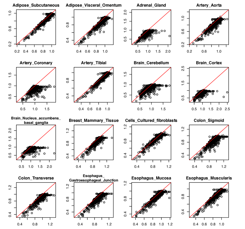
Figure 1: Scatter plots of PMSEs in various tissues. Y-axis: PMSE of the proposed method. X-axis: PMSE of the OLS.

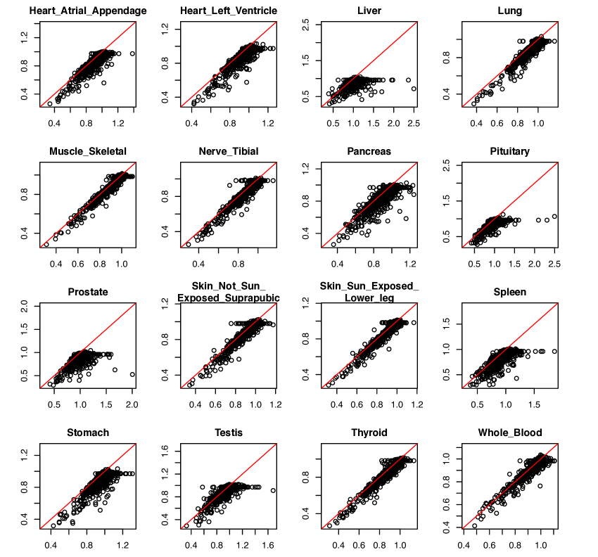
Figure 2: Scatter plots of PMSEs in various tissues. Y-axis: PMSE of the proposed method. X-axis: PMSE of the OLS.

For each tissue type, we also calculate the average increment and the percentage of the average increment of $R^{2}$ by the proposed method compared with the OLS method across all the genes. We provide these comparison results for all the tissues in Figure 3. Note that the proposed method substantially increases the average $R^{2}$ in all the tissues compared to the OLS method, which indicates that the proposed method produces the predicted values more correlated to the true gene expression values. On average, the proposed method improves the $R^{2}$ by $27.5\%$ across all the tissue types. In particular, for the artery coronary tissue, the proposed method increases the $R^{2}$ by more than $40\%$. When we only consider genes with at least $20$ cis-SNPs, the percentage of average increase of $R^{2}$ by the proposed method is over $80\%$ in the artery coronary tissue.

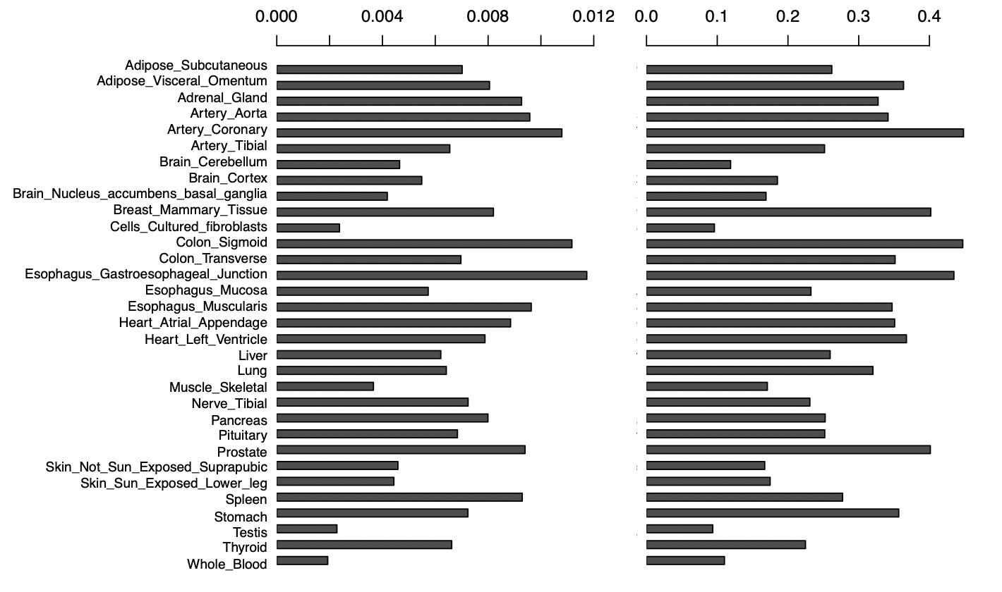
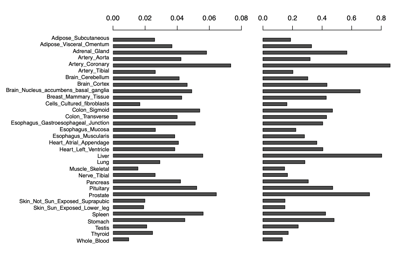
Figure 3: Increase of $R^{2}$ by the proposed method compared with the OLS method. Top left: Average increase of $R^{2}$ by the proposed method. Top right: Percentage of average increase of $R^{2}$ by the proposed method. Bottom left: Average increase of $R^{2}$ for genes with at least $20$ cis-SNPs by the proposed method. Bottom right: Percentage of average increase of $R^{2}$ for genes with at least $20$ cis-SNPs by the proposed method.

7.2 Posterior probability of cis-SNP gene expression association

In this subsection, we apply the proposed method to the whole dataset, and calculate the posterior probability of $I^{(t)}=1$ for $t=1,\dots,m$ and all the genes. This posterior probability indicates whether the cis-SNPs of a given gene have effects on the corresponding gene expression in a particular tissue based on the observed data. We use the “gplots” R package (https://cran.r-project.org/web/packages/gplots/index.html) to generate a heat map for all the posterior probabilities, where each column represents a tissue and each row represents a gene. We first note that for many genes, the cis-SNP and gene expression associations are observed all the tissues (top blue rows). There are only a few genes that do not have their corresponding cis-SNPs in all the tissues (bottom red rows). For many other genes, we observe tissue-specific cis-SNP gene expression associations, but for most of these genes, the cis-SNP associations are observed in most of the tissues.

As shown in Figure 4, the heat map clusters similar genes and similar tissues together based on the posterior probability of observing cis-SNP and gene expression association. We observe that the tissues that are clustered together are indeed For example, the “Esimilar. sophagus_Gastroesophageal_Junction” tissue and the “Esophagus_Muscularis” tissue are clustered together in Figure 4. They are both related to the esophagus. Similarly, the “Artery_Tibial”, “Artery_Coronary”, and “Artery_Aorta” tissues are all related to the artery and are clustered together in the heat map. Thus, the posterior probabilities based on the proposed method indeed capture the similarity between tissues in terms of the relationship between gene expression and cis-SNPs.

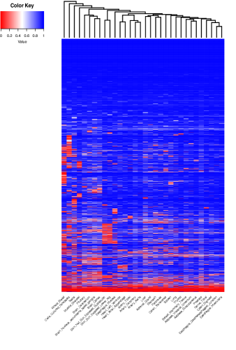
Figure 4: Posterior probabilities of $I^{(t)}=1$ for all the genes and tissues.

8 Discussion

We develop a new empirical Bayes regression model for multi-tissue eQTL analysis using the GTEx data, which improves the single tissue analysis produced by the traditional ordinary least squares method. To borrow information across tissues, the proposed method assigns a common mixture prior distribution to the cis-SNP effects in each tissue, and estimates parameters in the prior distribution through maximizing marginal likelihood of the expression levels in all the tissues. In addition, the method provides a way of quantify the evidence whether the cis-SNPs are “active” or not in a certain tissue based on the posterior probabilities of the latent configuration indicator in the mixture prior distribution. We apply the EM algorithm to find the maximum likelihood estimate of prior parameters. Moreover, to accommodate real data with missing responses such as the GTEx data, we have also developed the empirical Bayes estimator and the corresponding asymptotic results when there are missing data.

Theoretically, we have shown that the proposed estimator is asymptotically superior than the OLS estimator in terms of the Bayes risk. This superiority is mainly due to that the OLS only uses single tissue information while the proposed method incorporates common information from other tissues. In addition, the application to the GTEx data illustrates that the proposed method estimates the tissue-specific cis-SNP effects more accurately than the OLS method. More importantly, the proposed method provides posterior probabilities of whether there is cis-effects or not for each tissue, which indeed reflects similarity among tissues. For instance, the “Artery_Tibial”, “Artery_Coronary”, and “Artery_Aorta” tissues are shown to have similar cis-SNP gene expression association among all the genes.

In general, the empirical Bayes method provides a powerful framework for pooling information across multiple experiments or sources, and improving the accuracy of the estimation or inference in each experiment. Besides the SNP-gene association, we can also extend the empirical Bayes framework to improve the estimation of the relationship between expression levels of genes for the GTEx project where gene expression levels are measured over multiple tissues. For example, we could incorporate information across tissues through estimating a common prior on the multiple precision matrices for the multiple tissues. In addition, in this article, we mainly consider the association between gene expression and cis-SNPs. It would be of great interest to incorporate more covariates, including not only cis-SNPs but also trans-SNPs, in future research. We could involve penalty functions when the number of covariates exceeds the number of subjects.

SUPPLEMENTARY MATERIALS

The online Supplemental Materials include EM algorithm for missing data case, additional simulations and proofs of Theorems 1-3.

References

- Bhadra and Mallick (2013) {barticle}[author] \bauthor\bsnmBhadra, \bfnmAnindya\binitsA. and \bauthor\bsnmMallick, \bfnmBani K\binitsB. K. (\byear2013). \btitleJoint high-dimensional Bayesian variable and covariance selection with an application to eQTL analysis. \bjournalBiometrics \bvolume69 \bpages447–457. \endbibitem
- Brem et al. (2005) {barticle}[author] \bauthor\bsnmBrem, \bfnmRachel B\binitsR. B., \bauthor\bsnmStorey, \bfnmJohn D\binitsJ. D., \bauthor\bsnmWhittle, \bfnmJacqueline\binitsJ. and \bauthor\bsnmKruglyak, \bfnmLeonid\binitsL. (\byear2005). \btitleGenetic interactions between polymorphisms that affect gene expression in yeast. \bjournalNature \bvolume436 \bpages701–703. \endbibitem
- Consortium et al. (2017) {barticle}[author] \bauthor\bsnmConsortium, \bfnmGTEx\binitsG. \betalet al. (\byear2017). \btitleGenetic effects on gene expression across human tissues. \bjournalNature \bvolume550 \bpages204–213. \endbibitem
- Dempster, Laird and Rubin (1977) {barticle}[author] \bauthor\bsnmDempster, \bfnmArthur P\binitsA. P., \bauthor\bsnmLaird, \bfnmNan M\binitsN. M. and \bauthor\bsnmRubin, \bfnmDonald B\binitsD. B. (\byear1977). \btitleMaximum likelihood from incomplete data via the EM algorithm. \bjournalJournal of the Royal Statistical Society: Series B (Methodological) \bvolume39 \bpages1–22. \endbibitem
- Duong et al. (2016) {barticle}[author] \bauthor\bsnmDuong, \bfnmDat\binitsD., \bauthor\bsnmZou, \bfnmJennifer\binitsJ., \bauthor\bsnmHormozdiari, \bfnmFarhad\binitsF., \bauthor\bsnmSul, \bfnmJae Hoon\binitsJ. H., \bauthor\bsnmErnst, \bfnmJason\binitsJ., \bauthor\bsnmHan, \bfnmBuhm\binitsB. and \bauthor\bsnmEskin, \bfnmEleazar\binitsE. (\byear2016). \btitleUsing genomic annotations increases statistical power to detect eGenes. \bjournalBioinformatics \bvolume32 \bpagesi156–i163. \endbibitem
- Duong et al. (2017) {barticle}[author] \bauthor\bsnmDuong, \bfnmDat\binitsD., \bauthor\bsnmGai, \bfnmLisa\binitsL., \bauthor\bsnmSnir, \bfnmSagi\binitsS., \bauthor\bsnmKang, \bfnmEun Yong\binitsE. Y., \bauthor\bsnmHan, \bfnmBuhm\binitsB., \bauthor\bsnmSul, \bfnmJae Hoon\binitsJ. H. and \bauthor\bsnmEskin, \bfnmEleazar\binitsE. (\byear2017). \btitleApplying meta-analysis to genotype-tissue expression data from multiple tissues to identify eQTLs and increase the number of eGenes. \bjournalBioinformatics \bvolume33 \bpagesi67–i74. \endbibitem
- Flutre et al. (2013) {barticle}[author] \bauthor\bsnmFlutre, \bfnmTimothée\binitsT., \bauthor\bsnmWen, \bfnmXiaoquan\binitsX., \bauthor\bsnmPritchard, \bfnmJonathan\binitsJ. and \bauthor\bsnmStephens, \bfnmMatthew\binitsM. (\byear2013). \btitleA statistical framework for joint eQTL analysis in multiple tissues. \bjournalPLoS Genet \bvolume9 \bpagese1003486. \endbibitem
- Gamazon et al. (2015) {barticle}[author] \bauthor\bsnmGamazon, \bfnmEric R\binitsE. R., \bauthor\bsnmWheeler, \bfnmHeather E\binitsH. E., \bauthor\bsnmShah, \bfnmKaanan P\binitsK. P., \bauthor\bsnmMozaffari, \bfnmSahar V\binitsS. V., \bauthor\bsnmAquino-Michaels, \bfnmKeston\binitsK., \bauthor\bsnmCarroll, \bfnmRobert J\binitsR. J., \bauthor\bsnmEyler, \bfnmAnne E\binitsA. E., \bauthor\bsnmDenny, \bfnmJoshua C\binitsJ. C., \bauthor\bsnmNicolae, \bfnmDan L\binitsD. L., \bauthor\bsnmCox, \bfnmNancy J\binitsN. J. \betalet al. (\byear2015). \btitleA gene-based association method for mapping traits using reference transcriptome data. \bjournalNature genetics \bvolume47 \bpages1091. \endbibitem
- Gosik et al. (2017) {barticle}[author] \bauthor\bsnmGosik, \bfnmKirk\binitsK., \bauthor\bsnmKong, \bfnmLan\binitsL., \bauthor\bsnmChinchilli, \bfnmVernon M\binitsV. M. and \bauthor\bsnmWu, \bfnmRongling\binitsR. (\byear2017). \btitleiFORM/eQTL: an ultrahigh-dimensional platform for inferring the global genetic architecture of gene transcripts. \bjournalBriefings in bioinformatics \bvolume18 \bpages250–259. \endbibitem
- Gusev et al. (2016) {barticle}[author] \bauthor\bsnmGusev, \bfnmAlexander\binitsA., \bauthor\bsnmKo, \bfnmArthur\binitsA., \bauthor\bsnmShi, \bfnmHuwenbo\binitsH., \bauthor\bsnmBhatia, \bfnmGaurav\binitsG., \bauthor\bsnmChung, \bfnmWonil\binitsW., \bauthor\bsnmPenninx, \bfnmBrenda WJH\binitsB. W., \bauthor\bsnmJansen, \bfnmRick\binitsR., \bauthor\bsnmDe Geus, \bfnmEco JC\binitsE. J., \bauthor\bsnmBoomsma, \bfnmDorret I\binitsD. I., \bauthor\bsnmWright, \bfnmFred A\binitsF. A. \betalet al. (\byear2016). \btitleIntegrative approaches for large-scale transcriptome-wide association studies. \bjournalNature genetics \bvolume48 \bpages245–252. \endbibitem
- Hu et al. (2019) {barticle}[author] \bauthor\bsnmHu, \bfnmYiming\binitsY., \bauthor\bsnmLi, \bfnmMo\binitsM., \bauthor\bsnmLu, \bfnmQiongshi\binitsQ., \bauthor\bsnmWeng, \bfnmHaoyi\binitsH., \bauthor\bsnmWang, \bfnmJiawei\binitsJ., \bauthor\bsnmZekavat, \bfnmSeyedeh M\binitsS. M., \bauthor\bsnmYu, \bfnmZhaolong\binitsZ., \bauthor\bsnmLi, \bfnmBoyang\binitsB., \bauthor\bsnmGu, \bfnmJianlei\binitsJ., \bauthor\bsnmMuchnik, \bfnmSydney\binitsS. \betalet al. (\byear2019). \btitleA statistical framework for cross-tissue transcriptome-wide association analysis. \bjournalNature genetics \bvolume51 \bpages568–576. \endbibitem
- Li et al. (2018) {barticle}[author] \bauthor\bsnmLi, \bfnmGen\binitsG., \bauthor\bsnmShabalin, \bfnmAndrey A\binitsA. A., \bauthor\bsnmRusyn, \bfnmIvan\binitsI., \bauthor\bsnmWright, \bfnmFred A\binitsF. A. and \bauthor\bsnmNobel, \bfnmAndrew B\binitsA. B. (\byear2018). \btitleAn empirical Bayes approach for multiple tissue eQTL analysis. \bjournalBiostatistics \bvolume19 \bpages391–406. \endbibitem
- Lonsdale et al. (2013) {barticle}[author] \bauthor\bsnmLonsdale, \bfnmJohn\binitsJ., \bauthor\bsnmThomas, \bfnmJeffrey\binitsJ., \bauthor\bsnmSalvatore, \bfnmMike\binitsM., \bauthor\bsnmPhillips, \bfnmRebecca\binitsR., \bauthor\bsnmLo, \bfnmEdmund\binitsE., \bauthor\bsnmShad, \bfnmSaboor\binitsS., \bauthor\bsnmHasz, \bfnmRichard\binitsR., \bauthor\bsnmWalters, \bfnmGary\binitsG., \bauthor\bsnmGarcia, \bfnmFernando\binitsF., \bauthor\bsnmYoung, \bfnmNancy\binitsN. \betalet al. (\byear2013). \btitleThe genotype-tissue expression (GTEx) project. \bjournalNature genetics \bvolume45 \bpages580–585. \endbibitem
- Stegle et al. (2012) {barticle}[author] \bauthor\bsnmStegle, \bfnmOliver\binitsO., \bauthor\bsnmParts, \bfnmLeopold\binitsL., \bauthor\bsnmPiipari, \bfnmMatias\binitsM., \bauthor\bsnmWinn, \bfnmJohn\binitsJ. and \bauthor\bsnmDurbin, \bfnmRichard\binitsR. (\byear2012). \btitleUsing probabilistic estimation of expression residuals (PEER) to obtain increased power and interpretability of gene expression analyses. \bjournalNature Protocols \bvolume7 \bpages500. \endbibitem
- Stouffer et al. (1949) {bbook}[author] \bauthor\bsnmStouffer, \bfnmSamuel A\binitsS. A., \bauthor\bsnmSuchman, \bfnmEdward A\binitsE. A., \bauthor\bsnmDeVinney, \bfnmLeland C\binitsL. C., \bauthor\bsnmStar, \bfnmShirley A\binitsS. A. and \bauthor\bsnmWilliams Jr, \bfnmRobin M\binitsR. M. (\byear1949). \btitleThe american soldier: Adjustment during army life.(studies in social psychology in world war ii), vol. 1. \bpublisherPrinceton Univ. Press. \endbibitem
- Stranger et al. (2007) {barticle}[author] \bauthor\bsnmStranger, \bfnmBarbara E\binitsB. E., \bauthor\bsnmNica, \bfnmAlexandra C\binitsA. C., \bauthor\bsnmForrest, \bfnmMatthew S\binitsM. S., \bauthor\bsnmDimas, \bfnmAntigone\binitsA., \bauthor\bsnmBird, \bfnmChristine P\binitsC. P., \bauthor\bsnmBeazley, \bfnmClaude\binitsC., \bauthor\bsnmIngle, \bfnmCatherine E\binitsC. E., \bauthor\bsnmDunning, \bfnmMark\binitsM., \bauthor\bsnmFlicek, \bfnmPaul\binitsP., \bauthor\bsnmKoller, \bfnmDaphne\binitsD. \betalet al. (\byear2007). \btitlePopulation genomics of human gene expression. \bjournalNature Genetics \bvolume39 \bpages1217–1224. \endbibitem
- Sul et al. (2013) {barticle}[author] \bauthor\bsnmSul, \bfnmJae Hoon\binitsJ. H., \bauthor\bsnmHan, \bfnmBuhm\binitsB., \bauthor\bsnmYe, \bfnmChun\binitsC., \bauthor\bsnmChoi, \bfnmTed\binitsT. and \bauthor\bsnmEskin, \bfnmEleazar\binitsE. (\byear2013). \btitleEffectively identifying eQTLs from multiple tissues by combining mixed model and meta-analytic approaches. \bjournalPLoS Genet \bvolume9 \bpagese1003491. \endbibitem
- Wang et al. (2016) {barticle}[author] \bauthor\bsnmWang, \bfnmJiebiao\binitsJ., \bauthor\bsnmGamazon, \bfnmEric R\binitsE. R., \bauthor\bsnmPierce, \bfnmBrandon L\binitsB. L., \bauthor\bsnmStranger, \bfnmBarbara E\binitsB. E., \bauthor\bsnmIm, \bfnmHae Kyung\binitsH. K., \bauthor\bsnmGibbons, \bfnmRobert D\binitsR. D., \bauthor\bsnmCox, \bfnmNancy J\binitsN. J., \bauthor\bsnmNicolae, \bfnmDan L\binitsD. L. and \bauthor\bsnmChen, \bfnmLin S\binitsL. S. (\byear2016). \btitleImputing gene expression in uncollected tissues within and beyond GTEx. \bjournalThe American Journal of Human Genetics \bvolume98 \bpages697–708. \endbibitem
- Zeng, Wang and Huang (2017) {barticle}[author] \bauthor\bsnmZeng, \bfnmPing\binitsP., \bauthor\bsnmWang, \bfnmTing\binitsT. and \bauthor\bsnmHuang, \bfnmShuiping\binitsS. (\byear2017). \btitleCis-SNPs set testing and predixcan analysis for gene expression data using linear mixed models. \bjournalScientific reports \bvolume7 \bpages1–11. \endbibitem