Higher-group structure in $2n$-dimensional axion-electrodynamics

Abstract

We investigate $2n$-dimensional axion electrodynamics for the purpose of exploring a higher-group structure underlying it. This is manifested as a Green-Schwarz transformation of the background gauge fields that couple minimally to the conserved currents. The $n=3$ case is studied most intensively. We derive the identities of correlation functions among the global symmetry generators by using a gauge transformation that maps two correlation functions with each other. A key ingredient in this computation is given by the Green-Schwarz transformation and the ’t Hooft anomalies associated with the gauge transformation. The algebraic structure of these results and its physical interpretations are discussed in detail. In particular, we find that the higher-group structure for $n=3$ is endowed with a multi-ary operation among the symmetry generators.

1 Introduction

Recent developments in studies of global symmetries have led to a deeper understanding of nonperturbartive aspects of quantum field theories(QFTs).

One of the most important results in this line is the use of higher-form symmetries [1] (see also Refs. [2, 3, 4, 5, 6, 7, 8, 9, 10, 11, 12]). $p$-form symmetry is characterized by a symmetry generator whose support is given by a manifold of codimension $p+1$, and which measures a charge carried by $p$-dimensional extended objects. Such symmetries have been applied to many contexts of quantum field theories, see e.g. [13, 14, 15, 16, 17, 18, 19, 20, 21, 22, 23, 24, 25, 26, 27, 28]. It may occur that transformation of a certain rank induces that of a different rank in a nontrivial manner. Such a mathematical structure is referred to as higher-group structure. For instance, 2-group structure [29] involves 0-form and 1-form symmetries, where the action of the 0-form symmetry generator on the 1-form symmetry generator gives rise to another 1-form symmetry generator. For a recent development of higher-group structure in the QFT context, see e.g. [11, 30, 31, 32, 33, 34, 35, 36, 37, 38, 39, 40, 41, 42, 43, 44, 45, 46, 47, 48, 49, 50, 51]. Mathematical formulation of higher-group structure is made by means of an extension of group to higher-category, see [52] for a review.

It has become clear that axion systems in four dimensions serve as a QFT model that encodes the physical and mathematical structures of higher-group in a simple but nontrivial manner. In particular, the papers [53, 54] show that the massless axion and Maxwell system exhibits a 3-group structure. When the axion and photon is massive, it enhances to a 4-group structure [55]. The higher-group structure in axion-Yang-Mills theories is discussed in [56]. The physical interpretation of the higher-group structures can be given via the Witten effect [57] and the anomalous Hall effect for the axion. Here, the Witten effect for the axion means that an axionic domain wall enclosing a magnetic monopole has an electric charge [58], and the anomalous Hall effect implies that there is an induced current when we add an electric field around an axionic string [59, 60, 61]. The purpose of this paper is to explore the higher-group structures of axion electrodynamics by extending it to a generic $2n$-dimensional spacetime.

Higher-group structures can be efficiently described in the presence of the background gauge fields coupled with the higher-form symmetry currents [37]. In [54], the 3-group structure is realized as a Green-Schwarz(GS)-type transformation [62] of the background gauge fields that are associated with Chern-Weil(CW) symmetry [49, 47]. The CW current is trivial in that the current conservation is satisfied by Bianchi identities, but plays a key role in understanding the 3-group structure. In fact, the background gauging of the symmetries associated with equations of motion(EoMs) for the axion and photon must require the simultaneous background gauging of CW symmetries with GS transformations enforced in order to preserve the gauge invariance of the axion and photon. It is then natural to expect that higher-dimensional axion electrodynamics exhibits enhanced algebraic structure compared to four dimensions, because it admits a larger number of CW currents.

In this paper, we study the higher-group structure of axion electrodynamics in $2n$ dimensions. The higher group is organized by the CW symmetries and the higher-form symmetries associated to the equation of motion. The 1-, 2-, $\cdots$, $(2n-2)$-form CW symmetries in the $2n$-dimensional axion electrodynamics must be gauged with the corresponding background gauge fields required to make a GS-type transformation in order to remove a quantum inconsistency due to operator-valued ambiguities when we gauge the higher-form symmetries based on the equations of motion. In particular, the $2n=6$ case is analyzed most intensively. It is found that a new algebraic structure emerges such that it contains the 3-group structure of the $2n=4$ case as a substructure with a trinary operation among three symmetry generators encoded in it.

The organization of this paper is as follows. Section 2 gives the action of the $2n$-dimensional axion and Maxwell theory and then derives the global symmetries of the system. It is found they are divided into two classes, one containing the symmetries whose current is conserved by the equations of motion(EoMs) and the other composed of the CW symmetry. In section 2.2, we introduce the background gauge fields for the global symmetries, and derive the GS-type transformation laws for the CW symmetry gauge fields. They are the manifestation of higher-group structure that contains the 3-group as a substructure. Section 3 focuses on the $2n=6$ case. Using the GS transformation laws derived in section 2.2, we compute some correlation functions among the symmetry generators of the 6-dimensional axion electrodynamics. Section 5 is devoted to a conclusion and discussion. In appendix A, we review a method developed in [53] for computing the correlation functions of the symmetry generators.

2 $2n$-dimensional axion electrodynamics

The action of axion electrodynamics in $2n$ dimensions is given by

$$S=-\int_{{\mathcal{M}}_{2n}}\left(\frac{v^{2}}{2}|d\phi|^{2}+\frac{1}{2e^{2}}|da|^{2}-\frac{N}{(2\pi)^{n}n!}\phi\,(da)^{n}\right)\ .$$ (2.1)

Here, $\phi$ is an axion field with the $2\pi$ periodicity $\phi\sim\phi+2\pi$ and $a=a_{\mu}dx^{\mu}$ an $U(1)$ 1-form gauge field with the Dirac quantization $\int_{\cal S}da\in 2\pi\mathbb{Z}$ for a closed 2-dimensional subspace ${\cal S}$. $N$ is quantized to be integer when ${\mathcal{M}}_{2n}$ is a spin manifold. We use the notation of differential forms. The symbol $d$ denotes the exterior derivative, and $\wedge$ is the wedge product. The kinetic term of a $p$-form field ${\cal X}$ is written in terms of $|{\mathcal{X}}|^{2}={\mathcal{X}}\wedge\star{\mathcal{X}}=\frac{1}{p!}{\cal X}^{\mu_{1}...\mu_{p}}{\cal X}_{\mu_{1}...\mu_{p}}d^{2n}x$ with $\star$ being the Hodge star. We sometimes abbreviate wedge products $\underbrace{da\wedge\cdots\wedge da}_{n}$ to $(da)^{n}$. $v$ is a dimensionful parameter of mass dimension $n-1$ and $e$ the $U(1)$ gauge coupling constant. For simplicity, we set $v=1$ and $e=1$ hereafter.

2.1 Symmetries

In this subsection, we find out the global symmetries of the action (2.1). As shown below, it possesses higher-form symmetries of any integer ranks, which are divided into two classes. One contains EoM-based discrete symmetries and the other consists of CW symmetries.

EoM-based global symmetries

The EoMs of $\phi$ and $a$ read

$$d\star d\phi=-\frac{N}{(2\pi)^{n}n!}(da)^{n}\ ,~{}~{}~{}d\star da=\frac{N}{(2\pi)^{n}(n-1)!}d\phi\wedge(da)^{n-1}\ .$$ (2.2)

The EoM of $\phi$ leads to the 0-form symmetry current

$$j_{\rm EoM}^{[0]}=-\star d\phi-\frac{N}{(2\pi)^{n}n!}a\wedge(da)^{n-1}\ .$$ (2.3)

This defines the discrete 0-form symmetry ${\mathbb{Z}}_{N}^{[0]}$. To see this, we note that the symmetry generator, which is given by exponentiating the current integrated over a $(2n-1)$-dimensional manifold, is gauge invariant if the rotation angle is ${\mathbb{Z}}_{N}$-valued:

$$U^{[0]}_{\rm EoM}({\mathcal{D}}_{2n-1},\frac{2\pi m}{N})=e^{\frac{2i\pi m}{N}\int_{{\mathcal{D}}_{2n-1}}j_{\rm EoM}^{[0]}}\ ,$$ (2.4)

with $m\in{\mathbb{Z}}$. Here, ${\mathcal{D}}_{2n-1}$ is a $(2n-1)$-dimensional closed subspace.

The EoM of the photon gives the current

$$j_{\rm EoM}^{[1]}=\star da-\frac{N}{(2\pi)^{n}(n-1)!}\phi(da)^{n-1}\ .$$ (2.5)

The Noether charge is obtained by integrating the current over a $(2n-2)$-dimensional manifold ${\mathcal{D}}_{2n-2}$ and generates the discrete 1-form symmetry ${\mathbb{Z}}_{N}^{[1]}$ with the symmetry generator given by

$$U^{[1]}_{\rm EoM}({\mathcal{D}}_{2n-2},\frac{2\pi m}{N})=e^{\frac{2i\pi m}{N}\int_{{\mathcal{D}}_{2n-2}}j_{\rm EoM}^{[1]}}\ .$$ (2.6)

Chern-Weil symmetries

The Chern-Weil symmetry currents are conserved because of the Bianchi identities. The model (2.1) has $2n$ CW currents, which generate $(-1)$-, 0-, $\cdots$, $(2n-2)$-form $U(1)$ symmetries. For an integer $r$ with $0\leq r\leq n-1$, the $2r$-form symmetry current is given by

$$j_{\rm CW}^{[2r]}=\frac{1}{(2\pi)^{n-r}(n-r-1)!}\,d\phi\wedge(da)^{n-r-1}\ .$$ (2.7)

Also the $(2r-1)$-form symmetry current is given by

$$j_{\rm CW}^{[2r-1]}=\frac{1}{(2\pi)^{n-r}(n-r)!}\,(da)^{n-r}\ .$$ (2.8)

These yield the higher-form $U(1)$ symmetry generator of rank $k=0,1,2,\cdots,2n-2$

$$U_{\rm CW}^{[k]}({\mathcal{D}}_{2n-k-1},\gamma)=e^{i\gamma\int_{{\mathcal{D}}_{2n-k-1}}j_{\rm CW}^{[k]}}\ ,$$ (2.9)

with $\gamma\in{\mathbb{R}}/2\pi{\mathbb{Z}}$.

2.2 Background gauging and ’t Hooft anomaly

Here, we gauge the higher-form symmetries by coupling the currents found in the previous subsection to background gauge fields. As found in [54], gauging ${\mathbb{Z}}_{N}^{[0]}$ and ${\mathbb{Z}}_{N}^{[1]}$ causes an operator-valued ambiguity, which states that the gauged action depends on how it is extended to an extra dimension in order to make it gauge invariant. This problem is resolved by requiring that the background gauge fields for the CW symmetries transform under the ${\mathbb{Z}}_{N}^{[0]}$ and ${\mathbb{Z}}_{N}^{[1]}$ transformations in an appropriate manner.

We first gauge ${\mathbb{Z}}_{N}^{[1]}$, which acts on the photon field as

$$a\rightarrow a+\Lambda_{1}\ .$$ (2.10)

with $\Lambda_{1}$ being a 1-form gauge transformation function. We consider a background ${\mathbb{Z}}_{N}$ gauge field given by a set of 2- and 1-forms $(B_{2},B_{1})$ with $NB_{2}=dB_{1}$, which transform as

$$B_{2}\rightarrow B_{2}+d\Lambda_{1}\ ,~{}~{}\ B_{1}\rightarrow B_{1}+N\Lambda_{1}\ .$$ (2.11)

Here, $B_{1}$ is normalized as $\int_{\cal S}dB_{1}\in 2\pi\mathbb{Z}$ for a 2-dimensional closed surface ${\cal S}$. Then, $da$ in the action (2.1) should be replaced with $da-B_{2}$ in order to ensure that the action is gauge invariant. The gauged action is in conflict with the periodicity of the axion field $\phi\rightarrow\phi+2\pi$, however. This problem can be rephrased as an ambiguity of how to extend the action in the partition function defined on ${\mathcal{M}}_{2n}$ to the action defined on an artificial $(2n+1)$-dimensional manifold $\Omega_{{\mathcal{M}}_{2n}}$ with $\partial\Omega_{{\mathcal{M}}_{2n}}={\mathcal{M}}_{2n}$:

$$\frac{N}{(2\pi)^{n}n!}\int_{{\mathcal{M}}_{2n}}\phi(da-B_{2})^{n}=\frac{N}{(2\pi)^{n}n!}\int_{\Omega_{{\mathcal{M}}_{2n}}}d\phi\wedge(da-B_{2})^{n}\quad\text{mod }2\pi.$$ (2.12)

Hereafter, we omit writing “mod $2\pi$” for simplicity. For the purpose of computing the difference of the actions that arises from two choices of $(2n+1)$-manifolds $\Omega_{{\mathcal{M}}_{2n}}$ and $\Omega^{\prime}_{{\mathcal{M}}_{2n}}$, we define a closed manifold ${\mathcal{Z}}_{2n+1}=\Omega_{{\mathcal{M}}_{2n}}\sqcup\overline{\Omega^{\prime}_{{\mathcal{M}}_{2n}}}$ and evaluate the gauged topological action on it. Here, $\overline{\Omega^{\prime}_{{\mathcal{M}}_{2n}}}$ is $\Omega^{\prime}_{{\mathcal{M}}_{2n}}$ with an opposite orientation. By expanding it as

$$\frac{N}{(2\pi)^{n}n!}\int_{\Omega_{{\mathcal{M}}_{2n}}}d\phi\wedge(da-B_{2})^{n}=\frac{N}{(2\pi)^{n}}\sum_{k=0}^{n}\frac{(-1)^{n-k}}{k!(n-k)!}\int_{\Omega_{{\mathcal{M}}_{2n}}}d\phi\wedge(da)^{k}\wedge(B_{2})^{n-k}$$ (2.13)

only the 0th and 1st order terms in $B_{2}$ take values in $2\pi{\mathbb{Z}}$ because of the normalization condition $N\int B_{2}\in 2\pi{\mathbb{Z}}$. The operator-valued ambiguities originate from the rest of the terms that are nonlinear in $B_{2}$.

We now show that the quantum ambiguities can be eliminated by adding the local counterterms

$$\sum_{r=1}^{n-1}\int_{\Omega_{{\mathcal{M}}_{2n}}}j_{{\rm CW}}^{[2r]}\big{|}_{da\to da-B_{2}}\wedge Y_{2r+2}$$

$$= \sum_{k=0}^{n-2}\int_{\Omega_{{\mathcal{M}}_{2n}}}d\phi\,(da)^{k}\sum_{r=1}^{n-k-1}\frac{(-1)^{n-k-r}}{(2\pi)^{n-r}k!(n-k-r-1)!}(B_{2})^{n-r-k-1}\wedge Y_{2r+2}\ .$$ (2.14)

The replacement $da\to da-B_{2}$ should be made in order to keep the counterterm term invariant under the ${\mathbb{Z}}_{N}^{[1]}$ gauge transformation. It is interesting to note that no replacement is necessary for the four-dimensional axion-Maxwell system because the quantum ambiguities for the $2n=4$ case that involve the axion field are independent of $da$. This is manifest also upon setting $n=2$ in (2.14). $Y_{2r+2}$ is a $(2r+2)$-form field strength of the form $Y_{2r+2}=dX_{2r+1}+\alpha_{2r+2}$. $X_{2r+1}$ is the background CW gauge field that couples minimally with the current $j_{\rm CW}^{[2r]}$ with the normalization condition given by $\int dX_{2r+1}\in 2\pi{\mathbb{Z}}$. $\alpha_{2r+2}$ is fixed by requiring that the local counter terms cancel the operator-valued ambiguities from the gauged topological term. To see this, we note that adding (2.14) to the topological term (2.12) gives the integrand

$$\sum_{k=0}^{n-2}\frac{1}{(2\pi)^{k+1}\,k!}\,d\phi\,(da)^{k}$$

$$\qquad\wedge\left[2\pi N\,\frac{(-1)^{n-k}}{(2\pi)^{n-k}\,(n-k)!}(B_{2})^{n-k}\right.$$

$$\left.\hphantom{\qquad\wedge\qquad}-\sum_{r=1}^{n-k-1}\frac{(-1)^{n-k-r-1}}{(2\pi)^{n-k-r-1}\,(n-k-r-1)!}\,(B_{2})^{n-k-r-1}\wedge Y_{2r+2}\right]$$

$$+ \frac{N}{(2\pi)^{n}}\sum_{k=n-1}^{n}\frac{(-1)^{n-k}}{k!(n-k)!}d\phi\,(da)^{k}\,(B_{2})^{n-k}.$$ (2.15)

The operator-valued ambiguities can be cancelled by requiring

$$2\pi N\,\frac{(-1)^{n-k}}{(2\pi)^{n-k}\,(n-k)!}(B_{2})^{n-k}-\sum_{r=1}^{n-k-1}\frac{(-1)^{n-k-r-1}}{(2\pi)^{n-k-r-1}\,(n-k-r-1)!}\,(B_{2})^{n-k-r-1}\wedge Y_{2r+2}$$

$$=-dX_{2(n-k)-1}\ ,$$ (2.16)

for $k=0,1,2,\cdots,n-2$. This allows us to fix $\alpha_{2r+2}$ completely. We start examining the cancellation condition from the $k=n-2$ case to obtain $\alpha_{4}=\frac{N}{4\pi}(B_{2})^{2}$. The rest of $\alpha_{2r+2}$ can be worked out by solving the cancellation conditions for $k=n-3,n-4,\cdots,0$ recursively. As clear from the sample computation of $\alpha_{4}$, all $\alpha_{2r+2}$ are written in terms of $B_{2}$. Naively, this implies that $Y_{2r+2}$ is not ${\mathbb{Z}}_{N}^{[1]}$ gauge invariant so that the local counter terms break the ${\mathbb{Z}}_{N}^{[1]}$ gauge invariance. It is restored by requiring that $X_{2r+1}$ transform under ${\mathbb{Z}}_{N}^{[1]}$ in such a manner that $Y_{2r+2}$ is kept gauge invariant. This is the reason for why the GS-type transformation must be imposed for $X_{2r+1}$.

Furthermore, we gauge ${\mathbb{Z}}^{[0]}_{N}$, which acts on the axion as a shift:

$$\phi\rightarrow\phi+\Lambda_{0}\ .$$ (2.17)

The ${\mathbb{Z}}^{[0]}_{N}$ background gauge field is defined by a pair of 1- and 0-form fields $(A_{1},A_{0})$ with $NA_{1}=dA_{0}$, and the ${\mathbb{Z}}^{[0]}_{N}$ gauge transformation acts as

$$A_{1}\rightarrow A_{1}+d\Lambda_{0}\ ,~{}~{}\ A_{0}\rightarrow A_{0}+N\Lambda_{0}\ .$$ (2.18)

Here, $A_{0}$ is normalized as $\int_{\cal C}dA_{0}\in 2\pi\mathbb{Z}$ for a closed 1-dimensional subspace ${\cal C}$. The ${\mathbb{Z}}^{[0]}_{N}$ gauge invariant action is obtained by replacing $d\phi$ with the covariant derivative $d\phi-A_{1}$. Then, (2.15) together with (2.16) leads to the linear term in $A_{1}$:

$$\frac{1}{2\pi}\,A_{1}\wedge dX_{2n-1}+\sum_{k=1}^{n-2}\frac{1}{(2\pi)^{k+1}\,k!}\,A_{1}\wedge(da)^{k}\wedge dX_{2(n-k)-1}$$

$$\quad+\frac{N}{(2\pi)^{n}\,(n-1)!}\,A_{1}\wedge(da)^{n-1}\wedge B_{2}-\frac{N}{(2\pi)^{n}\,n!}\,A_{1}\wedge(da)^{n}\ .$$ (2.19)

It is clear that the second and the third terms are responsible for another quantum ambiguity. The first term is written only by the background field, resulting in an ’t Hooft anomaly. This ambiguity can be canceled by further adding the counterterms

$$\sum_{r=1}^{n-1}j_{{\rm CW}}^{[2r-1]}\big{|}_{da\to da-B_{2}}\wedge Y_{2r+1}$$

$$= \sum_{r=1}^{n-1}\frac{(-1)^{n-r}}{(2\pi)^{n-r}\,(n-r)!}(B_{2})^{n-r}\wedge Y_{2r+1}$$

$$+\sum_{k=1}^{n-1}\frac{1}{(2\pi)^{k}\,k!}(da)^{k}\sum_{r=1}^{n-k}\frac{(-1)^{n-k-r}}{(2\pi)^{n-k-r}\,(n-k-r)!}(B_{2})^{n-k-r}\wedge Y_{2r+1}\ ,$$ (2.20)

where $Y_{2r+1}=dX_{2r}+\alpha_{2r+1}$ with the normalization condition given by $\int dX_{2r+1}\in 2\pi{\mathbb{Z}}$. Adding it to (2.19) cancels the ambiguity by requiring that $\alpha_{2r+1}$ obey

$$dX_{2} =\frac{N}{2\pi}\,A_{1}\wedge B_{2}+Y_{3}\ ,$$ (2.21)

$$dX_{2(n-k)} =\frac{1}{2\pi}\,A_{1}\wedge dX_{2(n-k)-1}+\sum_{r=1}^{n-k}\frac{(-1)^{n-k-r}}{(2\pi)^{n-k-r}\,(n-k-r)!}\,(B_{2})^{n-k-r}\wedge Y_{2r+1}\ ,$$ (2.22)

for $k=1,2,\cdots,n-2$. (2.21) determines $\alpha_{3}$ and (2.22) can be solved recursively as before to fix the rest of $\alpha_{2r+1}$. For instance, the condition for $k=n-2$ is solved by setting

$$\alpha_{5}=-\frac{1}{2\pi}\,A_{1}\wedge dX_{3}+\frac{1}{2\pi}\,B_{2}\wedge\left(dX_{2}-\frac{N}{2\pi}\,A_{1}\wedge B_{2}\right)\ .$$ (2.23)

It is found that $\alpha_{2r+1}$ is not gauge invariant either. The counterterm (2.20) is left gauge invariant by requiring that $X_{2r}$ make a GS-type transformation under ${\mathbb{Z}}_{N}^{[0]}$ and ${\mathbb{Z}}_{N}^{[1]}$ in such a manner that $Y_{2r+1}$ becomes a gauge invariant field strength.

To summarize, the gauge invariant action with no operator-valued ambiguity is given by

$$S^{\prime}= -\int_{{\mathcal{M}}_{2n}}\left(\frac{1}{2}|d\phi-A_{1}|^{2}+\frac{1}{2}|da-B_{2}|^{2}\right)$$

$$+\frac{N}{(2\pi)^{n}n!}\int_{\Omega_{{\mathcal{M}}_{2n}}}(d\phi-A_{1})\wedge(da-B_{2})^{n}+\sum_{r=1}^{2n-2}\int_{\Omega_{{\mathcal{M}}_{2n}}}j_{\rm CW}^{[r]}\Big{|}_{d\phi\to d\phi-A_{1},\,da\to da-B_{2}}\wedge Y_{r+2}\ .$$ (2.24)

This might depend on the choice of ${\Omega_{{\mathcal{M}}_{2n}}}$, which is used to rewrite Chern-Simons(CS) terms in a gauge invariant manner. The difference of the actions for two choices of $\Omega_{{\mathcal{M}}_{2n}}$ is manifested as a ’t Hooft anomaly. More concretely, we define the compact $(2n+1)$-dimensional manifold ${\mathcal{Z}}_{2n+1}$ such that ${\mathcal{Z}}_{2n+1}=\Omega_{{\mathcal{M}}_{2n}}^{(1)}\cup\overline{\Omega_{{\mathcal{M}}_{2n}}^{(2)}}$, where $\Omega_{{\mathcal{M}}_{2n}}^{(1)}$ and $\Omega_{{\mathcal{M}}_{2n}}^{(2)}$ are glued together at the common boundary $\partial\Omega_{{\mathcal{M}}_{2n}}^{(1)}=\partial\Omega_{{\mathcal{M}}_{2n}}^{(2)}={\mathcal{M}}_{2n}$. Then, the ’t Hooft anomaly is given by a phase in the partition function,

$$\exp i\int_{{\mathcal{Z}}_{2n+1}}\left[\frac{1}{2\pi}A_{1}\wedge dX_{2n-1}+\sum_{r=1}^{n-1}\frac{(-1)^{n-r}}{(2\pi)^{n-r}\,(n-r)!}\,(B_{2})^{n-r}\wedge Y_{2r+1}\right]\ .$$ (2.25)

Here, the integrand comes from the terms in (2.24) that depend only on the background gauge field. If ${\mathcal{Z}}_{2n+1}$ is taken to be a mapping torus that interpolates between two ${\mathcal{M}}_{2n}$, each of which is endowed with background gauge fields related to each other via a gauge transformation, the phase (2.25) leads to an anomalous phase associated with the gauge transformation.

The explicit form of the ’t Hooft anomaly for the $n=3$ case is given in the next section.

3 The $n=3$ case

In this section, we make a detailed analysis of axion electrodynamics in six dimensions. This is in parallel with that made in [53, 54] for the $2n=4$ case.

The action in the absence of the background gauge field reads

$$S_{\rm 6d}=-\int_{{\mathcal{M}}_{6}}\left(\frac{1}{2}\left|d\phi\right|^{2}+\frac{1}{2}\left|da\right|^{2}-\frac{N}{48\pi^{3}}\phi\left(da\right)^{3}\right)\ .$$ (3.1)

Here, we briefly discuss the Witten effect induced on an axionic domain wall and the anomalous Hall effect by an axionic vortex. A more rigorous analysis will be given later. The EoMs for $\phi$ and $a$ are given in component by

$$\partial^{2}\phi =-\frac{N}{384\pi^{2}}\epsilon^{\mu\nu\rho\sigma\alpha\beta}F_{\mu\nu}F_{\rho\sigma}F_{\alpha\beta}\ ,$$ (3.2)

$$\partial_{\mu}F^{\mu\nu} =\frac{N}{64\pi^{2}}\epsilon^{\nu\rho\sigma\tau\alpha\beta}(\partial_{\rho}\phi)F_{\sigma\tau}F_{\alpha\beta}\ .$$ (3.3)

Assuming that $F_{\mu\nu}$ is static, the EoM (3.3) for $\nu=0$ gives

$$\partial_{i}F^{i0}=\frac{N}{64\pi^{2}}\epsilon^{0ijklm}(\partial_{i}\phi)F_{jk}F_{lm}\ ,$$

with $i,j,k,\cdots$ being the indices for the spatial directions. By turning on a domain wall configuration for $\phi$ together with a magnetic flux over the spatial direction of the domain wall, the RHS serves as an electric charge density induced on the domain wall. This is the Witten effect.

The EoM (3.3) for $\nu=m$ becomes

$$\partial_{n}F^{nm}=-\frac{N}{64\pi^{2}}\epsilon^{0ijklm}(\partial_{i}\phi)F_{0j}F_{kl}\ .$$

We give a vortex configuration to $\phi$, which appears as an axionic 3-brane. In addition, we turn on an electric field and a magnetic flux on the 3-brane world volume so that the RHS is nonvanishing. Then, the resultant source term serves as an electric current that flows towards the 3-brane, which is normal to the electric field direction.

The symmetries and the corresponding currents coupled minimally with the background gauge fields are listed as

Generator	Group	Current	Gauge field
$U_{\rm EoM}^{[0]}$	$\mathbb{Z}_{N}$	$j_{\rm EoM}^{[0]}=-\star d\phi-\frac{N}{48\pi^{3}}a\wedge da\wedge da$	$A_{1}$
$U_{\rm EoM}^{[1]}$	$\mathbb{Z}_{N}$	$j_{\rm EoM}^{[1]}=\star da-\frac{N}{16\pi^{3}}\phi\wedge da\wedge da$	$B_{2}$
$U_{\rm CW}^{[1]}$	$U(1)$	$j_{\rm CW}^{[1]}=\frac{1}{8\pi^{2}}da\wedge da$	$B_{2}^{\rm CW}$
$U_{\rm CW}^{[2]}$	$U(1)$	$j_{\rm CW}^{[2]}=\frac{1}{4\pi^{2}}d\phi\wedge da$	$C_{3}$
$U_{\rm CW}^{[3]}$	$U(1)$	$j_{\rm CW}^{[3]}=\frac{1}{2\pi}da$	$D_{4}$
$U_{\rm CW}^{[4]}$	$U(1)$	$j_{\rm CW}^{[4]}=\frac{1}{2\pi}d\phi$	$E_{5}$

Here, the gauge invariant field strengths $Y_{3},Y_{4},Y_{5},Y_{6}$ are renamed as $G_{3},H_{4},I_{5},J_{6}$ respectively:

$$G_{3} =dB_{2}^{\rm CW}-\frac{N}{2\pi}A_{1}\wedge B_{2},$$ (3.4)

$$H_{4} =dC_{3}+\frac{N}{4\pi}B_{2}\wedge B_{2},$$ (3.5)

$$I_{5} =dD_{4}-\frac{1}{2\pi}A_{1}\wedge dC_{3}+\frac{1}{2\pi}B_{2}\wedge dB_{2}^{\rm CW}-\frac{N}{4\pi^{2}}A_{1}\wedge B_{2}\wedge B_{2},$$ (3.6)

$$J_{6} =dE_{5}+\frac{1}{2\pi}B_{2}\wedge dC_{3}+\frac{N}{12\pi^{2}}B_{2}\wedge B_{2}\wedge B_{2},$$ (3.7)

As seen before, the gauge fields make a GS transformation in such a manner that these are left invariant under the ${\mathbb{Z}}_{N}^{[0]}$ and ${\mathbb{Z}}_{N}^{[1]}$ gauge transformations:

$$B_{2}^{\rm CW}\rightarrow B_{2}^{\rm CW}+d\Lambda_{1}^{\rm CW}-\frac{N}{2\pi}\left(A_{1}+d\Lambda_{0}\right)\wedge\Lambda_{1}+\frac{N}{2\pi}B_{2}\wedge\Lambda_{0}\ ,$$ (3.8)

$$C_{3}\rightarrow C_{3}+d\Lambda_{2}-\frac{N}{4\pi}\left(B_{2}+d\Lambda_{1}\right)\wedge\Lambda_{1}-\frac{N}{4\pi}B_{2}\wedge\Lambda_{1}\ ,$$ (3.9)

$$D_{4}\rightarrow D_{4}+d\Lambda_{3}-\frac{1}{2\pi}d\Lambda_{0}\wedge C_{3}-\frac{1}{2\pi}d\Lambda_{1}\wedge B_{2}^{\rm CW}$$

$$-\frac{N}{8\pi^{2}}\left(d\Lambda_{1}\wedge(B_{2}+d\Lambda_{1})\wedge d\Lambda_{0}+d\Lambda_{1}\wedge A_{1}\wedge d\Lambda_{1}+d\Lambda_{1}\wedge B_{2}\wedge d\Lambda_{0}\right)\ ,$$ (3.10)

$$E_{5}\rightarrow E_{5}+d\Lambda_{4}-\frac{N}{8\pi^{2}}B_{2}\wedge\left(B_{2}+d\Lambda_{1}\right)\wedge\Lambda_{1}-\frac{N}{12\pi^{2}}d\Lambda_{1}\wedge d\Lambda_{1}\wedge\Lambda_{1}$$

$$-\frac{1}{2\pi}d\Lambda_{1}\wedge C_{3}+\frac{N}{8\pi^{2}}(B_{2}+d\Lambda_{1})^{2}\wedge\Lambda_{1}\ .$$ (3.11)

The partition function of the 6d axion-Maxwell system, which is a functional of the background gauge fields, is given by

$$Z[A_{1},B_{2},B_{2}^{\rm CW},C_{3},D_{4},E_{5}]=\int{\mathcal{D}}\phi\,{\mathcal{D}}a\,\exp i\left[S_{\rm 6d}+S_{\rm min}+\int_{\Omega_{{\mathcal{M}}_{6}}}{\mathcal{L}}_{7}\right]\ ,$$ (3.12)

with

$$S_{\rm min}=\int_{{\mathcal{M}}_{6}}\left(j_{\rm EoM}^{[0]}\wedge A_{1}+j_{\rm EoM}^{[1]}\wedge B_{2}+j_{\rm CW}^{[1]}\wedge B_{2}^{\rm CW}+j_{\rm CW}^{[2]}\wedge C_{3}+j_{\rm CW}^{[3]}\wedge D_{4}+j_{\rm CW}^{[4]}\wedge E_{5}\right)\ ,$$ (3.13)

$${\mathcal{L}}_{7}=\frac{N}{16\pi^{3}}A_{1}\wedge(B_{2})^{3}-\frac{1}{8\pi^{2}}(B_{2})^{2}\wedge dB_{2}^{\rm CW}+\frac{1}{4\pi^{2}}A_{1}\wedge B_{2}\wedge dC_{3}-\frac{1}{2\pi}B_{2}\wedge dD_{4}+\frac{1}{2\pi}A_{1}\wedge dE_{5}\ .$$ (3.14)

Here, the ’t Hooft anomaly for $n=3$ is determined by the difference of (3.14) due to two choices of $\Omega_{{\mathcal{M}}_{6}}$, see (2.25). The seagull terms proportional to $|B_{2}|^{2}$ and $|A_{1}|^{2}$ are omitted for simplicity because these are irrelevant to the rest of the discussions in this paper.

3.1 Charged objects

Here, we discuss what are objects charged under the global symmetries we found before, and then compute the charges explicitly. In [54, 53], these are obtained by computing correlation functions involving charged objects and symmetry generators. This method is reviewed in the appendix A. In this paper, we give an alternative prescription based on a systematic use of the background gauge fields. It is found that the global charges are worked out from the ’t Hooft anomaly.

3.1.1 EoM-based symmetries

We first identify charged objects under the EoM-based global symmetries ${\mathbb{Z}}_{N}^{[0]}$ and ${\mathbb{Z}}_{N}^{[1]}$.

${\mathbb{Z}}_{N}^{[0]}$ acts on $\phi$ as a shift so that the associated charged object is given by a local operator ${\mathsf{I}}({\mathcal{P}}_{\rm defect},q)\equiv e^{iq\phi({\mathcal{P}}_{\rm defect})}$. Here, ${\mathcal{P}}_{\rm defect}$ is a point in the spacetime ${\cal M}_{6}$ on which the local operator is localized with $q\in{\mathbb{Z}}$ being the ${\mathbb{Z}}_{N}^{[0]}$ charge. Using

$$e^{iq\phi({\mathcal{P}}_{\rm defect})}=e^{2\pi iq\int j_{\rm CW}^{[4]}\wedge\delta_{5}(\Omega_{{\mathcal{P}}_{\rm defect}})}\ ,$$

the local operator arises by turning on $E_{5}=2\pi q\delta_{5}(\Omega_{{\mathcal{P}}})$. Here, the delta function $\delta_{p}({\mathcal{D}}_{D-p})$ with the support ${\mathcal{D}}_{D-p}$ being a submanifold of codimension $p$ is defined to satisfy

$$\int_{{\mathcal{M}}_{D}}J^{(D-p)}\wedge\delta_{p}({\mathcal{D}}_{D-p})\equiv\int_{{\mathcal{D}}_{D-p}}J^{(D-p)}\ ,$$

for any $(D-p)$-form $J^{(D-p)}$. Use of the Stokes theorem yields $\delta_{p}({{\mathcal{D}}}_{D-p})=(-1)^{D-p-1}d\delta_{p-1}(\Omega_{{{\mathcal{D}}}_{D-p}})$ with $\partial\Omega_{{{\mathcal{D}}}_{D-p}}={{\mathcal{D}}}_{D-p}$.

We now argue that the 0-form symmetry generator $U_{\rm EoM}^{[0]}({\mathcal{V}},2\pi n/N)$, which is supported on a codimension-one manifold ${\mathcal{V}}$, acts on ${\mathsf{I}}({\mathcal{P}}_{\rm defect},q)$ nontrivially. This is done by defining the correlation functions $\left\langle U_{\rm EoM}^{[0]}\left({\mathcal{V}},\frac{2\pi n}{N}\right){\mathsf{I}}\left({\mathcal{P}}_{\rm defect},q\right)\right\rangle$ and $\left\langle{\mathsf{I}}\left({\mathcal{P}}_{\rm defect},q\right)\right\rangle$ from the partition function (3.12) in the presence of the appropriate background gauge fields and then relating them with each other via the ’t Hooft anomaly. We define the correlator $\left\langle U_{\rm EoM}^{[0]}\left({\mathcal{V}},\frac{2\pi n}{N}\right){\mathsf{I}}\left({\mathcal{P}}_{\rm defect},q\right)\right\rangle$ by inserting $A_{1}=\frac{2\pi n}{N}\delta_{1}({\mathcal{V}})$ and $E_{5}=2\pi q\delta_{5}(\Omega_{{\mathcal{P}}_{\rm defect}})$ into (3.12):

$$\left\langle U_{\rm EoM}^{[0]}\left({\mathcal{V}},\frac{2\pi n}{N}\right){\mathsf{I}}\left({\mathcal{P}}_{\rm defect},q\right)\right\rangle\ \equiv Z\left[\frac{2\pi n}{N}\delta_{1}({\mathcal{V}}),0,0,0,0,2\pi q\delta_{5}(\Omega_{{\mathcal{P}}_{\rm defect}})\right]\ .$$ (3.15)

Note that $A_{1}=\frac{2\pi n}{N}\delta_{1}({\mathcal{V}})$ leads to a codimension-1 defect, which is referred to as an axionic domain wall. The relation between the axionic domain wall and $U_{\rm EoM}^{[0]}\left({\mathcal{V}},\frac{2\pi n}{N}\right)$ will be important later. We next make a gauge transformation to gauge away $A_{1}$, which amounts to eliminating $U_{\rm EoM}^{[0]}\left({\mathcal{V}},\frac{2\pi n}{N}\right)$. It follows from (3.8)-(3.11) that this induces no CW gauge fields. Then, there remains only $E_{5}$, in the presence of which the partition function defines $\left\langle{\mathsf{I}}\left({\mathcal{P}}_{\rm defect},q\right)\right\rangle$:

$$\left\langle{\mathsf{I}}\left({\mathcal{P}}_{\rm defect},q\right)\right\rangle\equiv Z[0,0,0,0,0,2\pi q\delta_{5}(\Omega_{{\mathcal{P}}_{\rm defect}})]\ .$$ (3.16)

Finally, we evaluate the ’t Hooft anomaly associated with the gauge transformation. As discussed in (2.25) and (3.14), it is obtained by integrating ${\mathcal{L}}_{7}$ over a mapping 7-torus ${\mathcal{T}}_{7}$ of topology ${\mathcal{M}}_{6}\times{\mathbb{S}}^{1}$, where $\mathbb{S}^{n}$ denotes a $n$-dimensional sphere. Let ${\mathcal{A}}_{1}$ and ${\mathcal{E}}_{5}$ be an lift of the background gauge field $A_{1}$ and $E_{5}$ respectively to ${\mathcal{T}}_{7}$ such that

$${\mathcal{A}}_{1}=(1-\tau)A_{1}\ ,~{}~{}~{}{\mathcal{E}}_{5}=E_{5}\ ,$$ (3.17)

with $\tau\in[0,1]$ being the coordinate of ${\mathbb{S}}^{1}$. It is easy to find that

$$\exp\left(i\int_{{\mathcal{T}}_{7}}{\mathcal{L}}_{7}\right)=\exp\left(\frac{i}{2\pi}\int_{{\mathcal{T}}_{7}}{\mathcal{A}}_{1}\wedge d{\mathcal{E}}_{5}\right)=\exp\left({\frac{2\pi iqn}{N}\int_{{\mathcal{M}}_{6}}\delta_{1}({\mathcal{V}})\wedge\delta_{5}(\Omega_{{\mathcal{P}}_{\rm defect}})}\right)\ .$$ (3.18)

The resultant phase factor measures the linking number between ${\mathcal{V}}$ and ${\mathcal{P}}_{\rm defect}$. We thus find that

$$\left\langle U_{\rm EoM}^{[0]}\left({\mathcal{V}},\frac{2\pi n}{N}\right){\mathsf{I}}\left({\mathcal{P}}_{\rm defect},q\right)\right\rangle=e^{\frac{2\pi iqn}{N}{\rm Link}\left(V,{\mathcal{P}}_{\rm defect}\right)}\left\langle{\mathsf{I}}\left({\mathcal{P}}_{\rm defect},q\right)\right\rangle\ .$$ (3.19)

The EoM-based 1-form symmetry ${\mathbb{Z}}_{N}^{[1]}$ acts on $a$ as a shift and gives rise to a nontrivial transformation for the Wilson loop ${\mathsf{W}}({\mathcal{L}}_{\rm defect},q)=e^{iq\int_{{\mathcal{L}}_{\rm defect}}a}$. By noting

$$e^{iq\int_{{\mathcal{L}}_{\rm defect}}a}=e^{2\pi iq\int j_{\rm CW}^{[3]}\wedge\delta_{4}(\Omega_{{\mathcal{L}}_{\rm defect}})}\ ,$$ (3.20)

the Wilson loop operator is realized by turning on $D_{4}=2\pi q\delta_{4}(\Omega_{{\mathcal{L}}_{\rm defect}})$. The partition function with $B_{2}=\frac{2\pi m}{N}\delta_{1}({\mathcal{W}})$ and $D_{4}=2\pi q\delta_{4}(\Omega_{{\mathcal{L}}_{\rm defect}})$ defines the correlator $\left\langle U_{\rm EoM}^{[1]}\left({\mathcal{W}},\frac{2\pi m}{N}\right){\mathsf{W}}\left({\mathcal{L}}_{\rm defect},q\right)\right\rangle$. By gauging away $B_{2}$ and evaluating the associated ’t Hooft anomaly, we obtain

$$\left\langle U_{\rm EoM}^{[1]}\left({\mathcal{W}},\frac{2\pi m}{N}\right){\mathsf{W}}\left({\mathcal{L}}_{\rm defect},q\right)\right\rangle=e^{\frac{2\pi iqm}{N}{\rm Link}\left({\mathcal{W}},{\mathcal{L}}_{\rm defect}\right)}\left\langle{\mathsf{W}}\left({\mathcal{L}}_{\rm defect},q\right)\right\rangle\ .$$ (3.21)

3.1.2 Chern-Weil symmetries

Here, we argue that the charged objects for the Chern-Weil symmetries are composed of axionic vortices and monopoles.

We first consider the 4-form symmetry generator $U^{[4]}_{\rm CW}({\mathcal{L}},\alpha)$ with ${\mathcal{L}}$ being a 1-dimensional support. As the corresponding CW current is given by $d\phi/(2\pi)$, the charged operator is realized by an axionic vortex, which is equivalent to turning on $A_{1}$ such that

$$\oint_{{\mathbb{S}}^{1}}A_{1,{\rm defect}}=2\pi q\ .$$ (3.22)

This defines the surface operator ${\mathsf{V}}({\mathcal{W}}_{\rm defect},q)$ with ${\mathcal{W}}_{\rm defect}$ being a codimension-2 support. This is also interpreted as an axionic 3-brane.

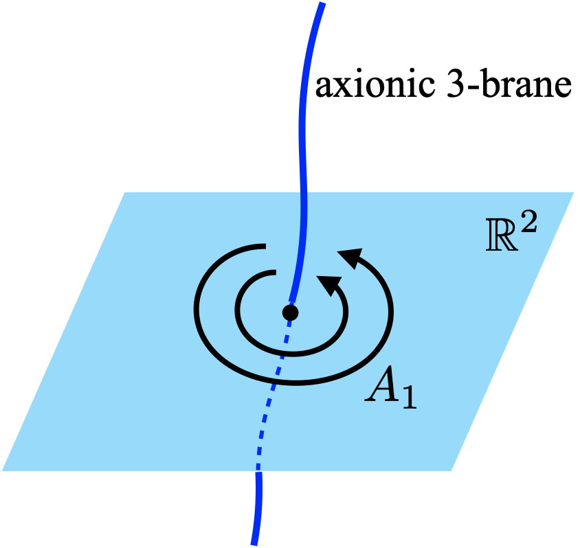
Figure 1: ${\mathsf{V}}({\mathcal{W}}_{\rm defect},q)$ as an axionic 3-brane carrying the $U^{[4]}_{\rm CW}$ charge

We verify that the $U_{\rm CW}^{[4]}$ charge of ${\mathsf{V}}({\mathcal{W}}_{\rm defect},q)$ is computed by evaluating the ’t Hooft anomaly in (3.14). The correlator $\left\langle U^{[4]}_{\rm CW}\left({\mathcal{L}},\alpha\right){\mathsf{V}}({\mathcal{W}}_{\rm defect},q)\right\rangle$ is defined from the partition function with $A=A_{1,{\rm defect}}$ and $E_{5}=\alpha\delta_{5}({\mathcal{L}})$:

$$Z[A_{1,{\rm defect}},0,0,0,0,\alpha\delta_{5}({\mathcal{L}})]=\left\langle U^{[4]}_{\rm CW}\left({\mathcal{L}},\alpha\right){\mathsf{V}}({\mathcal{W}}_{\rm defect},q)\right\rangle\ .$$ (3.23)

By making a gauge transformation to turn off $A_{1,{\rm defect}}$, we find

$$Z[A_{1,{\rm defect}},0,0,0,0,\alpha\delta_{5}({\mathcal{L}})]=e^{i\alpha q{\rm Link}({\mathcal{W}}_{\rm defect},{\mathcal{L}})}\,Z[0,0,0,0,0,\alpha\delta_{5}({\mathcal{L}})]\ .$$ (3.24)

Here, the phase factor in the RHS follows from the ’t Hooft anomaly, which is computed by constructing a mapping 7-torus associated with the gauge transformation under consideration. As the partition function in the RHS gives the one-point function of ${\mathsf{V}}({\mathcal{W}}_{\rm defect},q)$, we obtain

$$\langle U^{[4]}_{\rm CW}\left({\mathcal{L}},\alpha\right){\mathsf{V}}({\mathcal{W}}_{\rm defect},q)\rangle=e^{i\alpha q{\rm Link}({\mathcal{W}}_{\rm defect},{\mathcal{L}})}\,\langle{\mathsf{V}}({\mathcal{W}}_{\rm defect},q)\rangle\ .$$ (3.25)

Next, we discuss the 3-form symmetry generator $U^{[3]}_{\rm CW}({\mathcal{S}},\beta)$, which is supported on a codimension-4 manifold ${\mathcal{S}}$. As the corresponding CW current is $da/(2\pi)$, the charged object is a monopole. This is realized by turning on the background gauge field

$$\oint_{{\mathbb{S}}^{2}}B_{2,{\rm defect}}=2\pi q\ ,$$ (3.26)

and defines a codimension-3 surface operator ${\mathsf{T}}({\mathcal{C}}_{\rm defect},q)$ with ${\mathcal{C}}_{\rm defect}$ being the worldvolume. We call it an ’t Hooft surface.

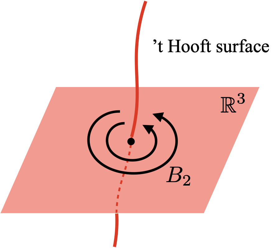
Figure 2: ’t Hooft surface operator ${\mathsf{T}}({\mathcal{C}}_{\rm defect},q)$ carrying the $U^{[3]}_{\rm CW}$ charge

The $U(1)^{[3]}$ charge of the ’t Hooft surface is computed from the ’t Hooft anomaly. For this purpose, we define the correlator of $U^{[3]}_{\rm CW}({\mathcal{S}},\beta)$ and ${\mathsf{T}}({\mathcal{C}}_{\rm defect},q)$ as the partition function in the presence of $B_{2,{\rm defect}}$ and $D_{4}=\beta\delta_{4}({\mathcal{S}})$:

$$Z[0,B_{2,{\rm defect}},0,0,D_{4}=\beta\delta_{4}({\mathcal{S}}),0]=\langle U^{[3]}_{\rm CW}\left({\mathcal{S}},\beta\right){\mathsf{T}}({\mathcal{C}}_{\rm defect},q)\rangle\ .$$ (3.27)

By gauging away $D_{4}$ and evaluating the associated ’t Hooft anomaly, we obtain

$$\langle U^{[3]}_{\rm CW}\left({\mathcal{S}},\beta\right){\mathsf{T}}({\mathcal{C}}_{\rm defect},q)\rangle=e^{i\beta q{\rm Link}({\mathcal{C}}_{\rm defect},{\mathcal{S}})}Z[0,B_{2,{\rm defect}},0,0,0,0]=e^{i\beta q{\rm Link}({\mathcal{C}}_{\rm defect},{\mathcal{S}})}\langle{\mathsf{T}}({\mathcal{C}}_{\rm defect},q)\rangle\ .$$ (3.28)

The charged operator for the 2-form symmetry $U(1)^{[2]}$ has a 2-dimensional worldvolume and is composed of an ’t Hooft surface and an axionic 3-brane wrapped around it, because the corresponding CW current is given by $d\phi\wedge da/(2\pi)^{2}$.

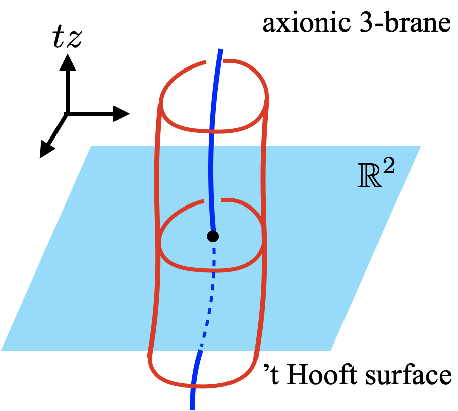
Figure 3: ${\mathsf{V}}{\mathsf{T}}({\mathcal{S}}_{\rm defect},q)$ carrying the $U^{[2]}_{\rm CW}$ charge

A typical configuration of the charged operator is listed below. Here, $r$ and $\vartheta$ are the polar coordinates of the 2-dimensional plane transverse to the axionic 3-brane.

	$t$	$x$	$y$	$z$	$r$	$\vartheta$
${\mathsf{V}}\left({\mathcal{W}}_{\rm defect},q_{\phi}\right)$	$\circ$	$\circ$	$\circ$	$\circ$
${\mathsf{T}}\left({\mathcal{C}}_{\rm defect},q_{a}\right)$	$\circ$			$\circ$		$\circ$

This is realized by turning on the background gauge fields $A_{1}$ and $B_{2}$ as

$$A_{1,{\rm defect}}=q_{\phi}d\vartheta\ ,~{}~{}~{}B_{2,{\rm defect}}=2\pi q_{a}\delta(x)\delta(y)\theta(r-\epsilon)dx\wedge dy\ ,$$ (3.29)

where $\epsilon>0$ is a regulator that is sent to zero eventually. It then follows that

$$\int A_{1,{\rm defect}}\wedge B_{2,{\rm defect}}=4\pi^{2}q\ ,~{}~{}~{}q=q_{\phi}q_{a}\ .$$ (3.30)

We define this configuration as an operator ${\mathsf{V}}{\mathsf{T}}({\mathcal{S}}_{\rm defect},q)$ with a 2-dimensional support ${\mathcal{S}}_{\rm defect}$ given by ${\mathbb{R}}^{2}\ni(t,z)$ and $q$ being the $U(1)^{[2]}$ charge. (3.30) is generalized to cases where ’t Hooft surfaces and axionic 3-branes are linked with each other on a slice with constant values of $(t,z)$.

The symmetry generator $U^{[2]}_{\rm CW}({\mathcal{L}},\gamma)$ that measures the charge of ${\mathsf{V}}{\mathsf{T}}({\mathcal{S}}_{\rm defect},q)$ is obtained by setting $C_{3}=\gamma\delta_{3}({\mathcal{L}})$, where ${\mathcal{L}}$ is a 3-dimensional surface that surrounds ${\mathcal{S}}_{\rm defect}$. This is verified by computing the correlation function of $U^{[2]}_{\rm CW}({\mathcal{L}},\gamma)$ and ${\mathsf{V}}{\mathsf{T}}({\mathcal{S}}_{\rm defect},q)$ following the same procedure as before:

$$\left\langle U^{[2]}_{\rm CW}\left({\mathcal{L}},\gamma\right){\mathsf{V}}{\mathsf{T}}({\mathcal{S}}_{\rm defect},q)\right\rangle=e^{i\gamma q{\rm Link}({\mathcal{S}}_{\rm defect},{\mathcal{L}})}\langle{\mathsf{V}}{\mathsf{T}}({\mathcal{S}}_{\rm defect},q)\rangle\ .$$ (3.31)

Finally, we consider the CW 1-form symmetry $U(1)^{[1]}$ and charged operators for it. By definition, these have a 1-dimensional support, and are composed of two ’t Hooft surfaces because the CW 1-form symmetry current is given by $(da)^{2}/(2\pi)^{2}$. A typical configuration for the charged operator is shown below:

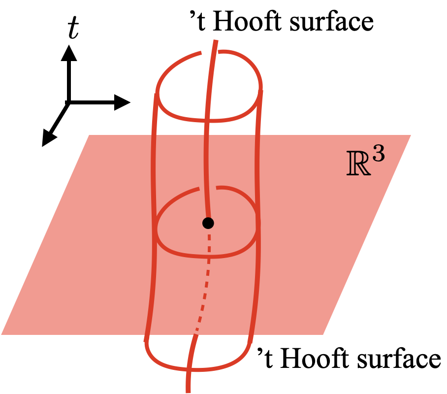
Figure 4: ${\mathsf{T}}{\mathsf{T}}({\mathcal{L}}^{\rm CW}_{\rm defect},q)$ carrying the $U^{[1]}_{\rm CW}$ charge

	$t$	$x$	$y$	$r$	$\vartheta$	$\varphi$
${\mathsf{T}}\left({\mathcal{C}}_{\rm defect},q\right)$	$\circ$	$\circ$	$\circ$
${\mathsf{T}}\left({\mathcal{C}}^{\prime}_{\rm defect},q^{\prime}\right)$	$\circ$				$\circ$	$\circ$

Here, $(r,\vartheta,\varphi)$ are the spherical coordinates of ${\mathbb{R}}^{3}$, which is transverse to ${\mathcal{C}}_{\rm defect}$. This configuration is realized by

$$B_{2,{\rm defect}}=\frac{q}{2}\sin\vartheta d\vartheta d\phi+2\pi q^{\prime}\delta(x)\delta(y)\theta(r-\epsilon)dxdy\ ,$$ (3.32)

and define the operator ${\mathsf{T}}{\mathsf{T}}({\mathcal{L}}^{\rm CW}_{\rm defect},q^{\prime\prime})$ with the 1-dimensional support ${\mathcal{L}}^{\rm CW}_{\rm defect}$ equal to ${\mathbb{R}}\ni t$ and $q^{\prime\prime}$ being the $U(1)^{[1]}$ charge evaluated from

$$\int B_{2,{\rm defect}}\wedge B_{2,{\rm defect}}=8\pi^{2}q^{\prime\prime}\ ,~{}~{}~{}q^{\prime\prime}=qq^{\prime}\ .$$ (3.33)

The symmetry generator $U^{[1]}_{\rm CW}\left({\mathcal{W}},\xi\right)$ for measuring ${\mathsf{T}}{\mathsf{T}}({\mathcal{L}}^{\rm CW}_{\rm defect},q^{\prime\prime})$ is realized by turning on $B_{2}^{\rm CW}=\xi\delta_{2}({\mathcal{W}})$ with $\xi$ being the $U(1)^{[1]}$ rotation angle and ${\mathcal{W}}$ a 4-dimensional support that surrounds ${\mathcal{L}}^{\rm CW}_{\rm defect}$. As before, the charge of ${\mathsf{T}}{\mathsf{T}}({\mathcal{L}}^{\rm CW}_{\rm defect},q)$ results from a ’t Hooft anomaly associated with a gauge transformation for removing $B_{2}^{\rm CW}$:

$$\left\langle U^{[1]}_{\rm CW}\left({\mathcal{W}},\xi\right){\mathsf{T}}{\mathsf{T}}({\mathcal{L}}^{\rm CW}_{\rm defect},q)\right\rangle=e^{i\xi q{\rm Link}({\mathcal{L}}^{\rm CW}_{\rm defect},{\mathcal{W}})}\langle{\mathsf{T}}{\mathsf{T}}({\mathcal{L}}^{\rm CW}_{\rm defect},q)\rangle\ .$$ (3.34)

3.2 Correlation functions of symmetry generators

In this subsection, we work out the identities among correlation function of the symmetry generators for the purpose of understanding the higher-group structures and their physical interpretation in the 6d axion-Maxwell system. A key ingredient in this analysis is the GS transformation laws for the CW gauge fields (3.8), (3.9), (3.10), (3.11). Part of the results given below is an extension of those obtained in [53, 54] for the 4d axion-Maxwell system.

3.2.1 Correlation functions of two EoM-based symmetry generators

We start discussing

$$Z\left[\frac{2\pi n}{N}\delta_{1}({\mathcal{V}}),\frac{2\pi m}{N}\delta_{2}({\mathcal{W}}),0,0,0,0\right] =\left\langle U_{\rm EoM}^{[0]}\left({\mathcal{V}},\frac{2\pi n}{N}\right)U_{\rm EoM}^{[1]}\left({\mathcal{W}},\frac{2\pi m}{N}\right)\right\rangle$$ (3.35)

with $A_{1}=\frac{2\pi n}{N}\delta_{1}({\mathcal{V}})$ and $B_{2}=\frac{2\pi m}{N}\delta_{2}({\mathcal{W}})$. We make a gauge transformation to gauge away $B_{2}$:

$$B_{2}\rightarrow B_{2}+d\Lambda_{1}=0\ ,~{}~{}~{}\Lambda_{1}=\frac{2\pi m}{N}\delta_{1}(\Omega_{\mathcal{W}})\ .$$ (3.36)

Note that this gauge transformation induces the CW gauge field $B_{2}^{\rm CW}$

$$B_{2}^{\rm CW}\rightarrow B_{2}^{\rm CW}-\frac{N}{2\pi}A_{1}\wedge\Lambda_{1}=-\frac{2mn}{N}\delta_{1}({\mathcal{V}})\wedge\delta_{1}(\Omega_{\mathcal{W}})\ ,$$ (3.37)

because of (3.8). It is easy to show that no ’t Hooft anomaly arises from the gauge transformation so that

$$Z\left[\frac{2\pi n}{N}\delta_{1}({\mathcal{V}}),\frac{2\pi m}{N}\delta_{2}({\mathcal{W}}),0,0,0,0\right]=Z\left[\frac{2\pi n}{N}\delta_{1}({\mathcal{V}}),0,-\frac{2\pi mn}{N}\delta_{1}({\mathcal{V}})\wedge\delta_{1}(\Omega_{\mathcal{W}}),0,0,0\right]\ .$$ (3.38)

Therefore,

$$\left\langle U_{\rm EoM}^{[0]}\left({\mathcal{V}},\frac{2\pi n}{N}\right)U_{\rm EoM}^{[1]}\left({\mathcal{W}},\frac{2\pi m}{N}\right)\right\rangle=\left\langle U_{\rm EoM}^{[0]}\left({\mathcal{V}},\frac{2\pi n}{N}\right)U_{\rm CW}^{[1]}\left({\mathcal{V}}\cap\Omega_{\mathcal{W}},-\frac{2\pi mn}{N}\right)\right\rangle\ .$$ (3.39)

The physical meaning of this relation becomes clearer by inserting the operator ${\mathsf{T}}{\mathsf{T}}({\mathcal{L}}^{\rm CW}_{\rm defect},q)$ into (3.39). Using (3.34), we obtain

$$\left\langle U_{\rm EoM}^{[0]}\left({\mathcal{V}},\frac{2\pi n}{N}\right)U_{\rm EoM}^{[1]}\left({\mathcal{W}},\frac{2\pi m}{N}\right){\mathsf{T}}{\mathsf{T}}({\mathcal{L}}^{\rm CW}_{\rm defect},q)\right\rangle$$

$$= e^{-i\frac{2\pi mnq}{N}{\rm Link}({\mathcal{L}}^{\rm CW}_{\rm defect},{\mathcal{V}}\cap\Omega_{\mathcal{W}})}\left\langle U_{\rm EoM}^{[0]}\left({\mathcal{V}},\frac{2\pi n}{N}\right){\mathsf{T}}{\mathsf{T}}({\mathcal{L}}^{\rm CW}_{\rm defect},q)\right\rangle\ .$$ (3.40)

As discussed in [53, 54], this can be interpreted as the Witten effect [57] induced on an axion domain wall. As a typical realization of (3.40), we consider

	$t$	$x$	$y$	$r$	$\vartheta$	$\varphi$
${\mathsf{T}}\left({\mathcal{C}}_{{\rm defect}1},q_{1}\right)$	$\circ$	$\circ$	$\circ$
${\mathsf{T}}\left({\mathcal{C}}_{{\rm defect}2},q_{2}\right)$	$\circ$			${\mathbb{S}}^{2}$
$U_{\rm EoM}^{[0]}\left({\mathcal{V}},\frac{2\pi n}{N}\right)$	$\circ$	$\circ$	$\circ$	${\mathbb{S}}^{2}$
$U_{\rm EoM}^{[1]}\left({\mathcal{W}},\frac{2\pi m}{N}\right)$		$\circ$	$\circ$	${\mathbb{S}}^{2}$

Here, ${\mathsf{T}}{\mathsf{T}}({\mathcal{L}}^{\rm CW}_{\rm defect},q)$ with $q=q_{1}q_{2}$ is composed of the two ’t Hooft surfaces as seen in Figure 4. A plot of this configuration at $t=0$, where $U_{\rm EoM}^{[1]}\left({\mathcal{W}},\frac{2\pi m}{N}\right)$ is localized, is shown in Figure 5.

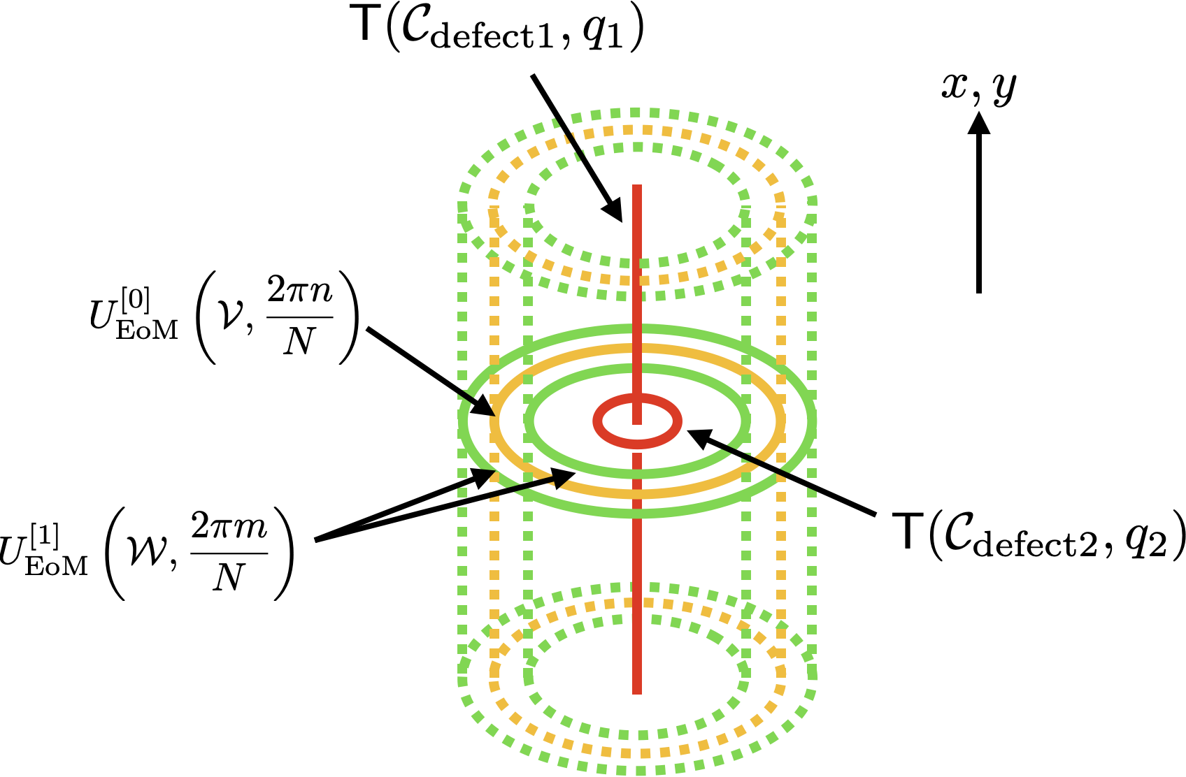
Figure 5: Witten effect on an axionic domain wall.

A magnetic field emanating from magnetic monopoles on the ’t Hooft surfaces goes through $U_{\rm EoM}^{[0]}\left({\mathcal{V}},\frac{2\pi n}{N}\right)$, which is regarded as an axionic domain wall with the worldvolume given by ${\mathcal{V}}$. The phase factor appearing in (3.40) implies the existence of an electric source induced on ${\mathcal{V}}$, because $U_{\rm EoM}^{[1]}\left({\mathcal{W}},\frac{2\pi m}{N}\right)$ is designed to measure an electric flux emanating from ${\mathcal{V}}$.

As a second example, we focus on the correlation function $\langle U_{\rm EoM}^{[1]}({\mathcal{W}}_{1},\frac{2\pi m_{1}}{N})\,U_{\rm EoM}^{[1]}({\mathcal{W}}_{2},\frac{2\pi m_{2}}{N})\rangle$. This is obtained by turning on $B_{2}=\frac{2\pi m_{1}}{N}\delta_{2}({\mathcal{W}}_{1})+\frac{2\pi m_{2}}{N}\delta_{2}({\mathcal{W}}_{2})$. Gauging away the second term in $B_{2}$ to remove $U_{\rm EoM}^{[1]}\left({\mathcal{W}}_{2},\frac{2\pi m_{1}}{N}\right)$ and then using the GS transformation law (3.9) gives

$$\left\langle U_{\rm EoM}^{[1]}\left({\mathcal{W}}_{1},\frac{2\pi m_{1}}{N}\right)U_{\rm EoM}^{[1]}\left({\mathcal{W}}_{2},\frac{2\pi m_{2}}{N}\right)\right\rangle=\left\langle U_{\rm EoM}^{[1]}\left({\mathcal{W}}_{1},\frac{2\pi m_{1}}{N}\right)U_{\rm CW}^{[2]}\left({\mathcal{W}}_{1}\cap\Omega_{{\mathcal{W}}_{2}},-\frac{2\pi m_{1}m_{2}}{N}\right)\right\rangle\ .$$ (3.41)

We now argue that this can be interpreted as an anomalous Hall effect in 6 dimensions. For this purpose, it is more convenient to insert the operator ${\mathsf{V}}{\mathsf{T}}({\mathcal{S}}_{\rm defect},q)$ into (3.41). By noting that ${\mathsf{V}}{\mathsf{T}}({\mathcal{S}}_{\rm defect},q)$ is charged under $U_{\rm CW}^{[2]}$, we find

$$\left\langle U_{\rm EoM}^{[1]}\left({\mathcal{W}}_{1},\frac{2\pi m_{1}}{N}\right)U_{\rm EoM}^{[1]}\left({\mathcal{W}}_{2},\frac{2\pi m_{2}}{N}\right){\mathsf{V}}{\mathsf{T}}({\mathcal{S}}_{\rm defect},q)\right\rangle$$

$$= e^{-i\frac{2\pi m_{1}m_{2}q}{N}{\rm Link}({\mathcal{S}}_{\rm defect},{\mathcal{W}}_{1}\cap\Omega_{{\mathcal{W}}_{2}})}\left\langle U_{\rm EoM}^{[1]}\left({\mathcal{W}}_{1},\frac{2\pi m_{1}}{N}\right){\mathsf{V}}{\mathsf{T}}({\mathcal{S}}_{\rm defect},q)\right\rangle\ .$$ (3.42)

A typical configuration for realizing the LHS of (3.42) is given below:

	$t$	$x$	$y$	$z$	$r$	$\vartheta$
${\mathsf{V}}\left({\mathcal{W}}_{\rm defect},q_{\phi}\right)$	$\circ$	$\circ$	$\circ$	$\circ$
${\mathsf{T}}\left({\mathcal{C}}_{\rm defect},q_{a}\right)$	$\circ$			$\circ$	${\mathbb{S}}^{1}$
$U_{\rm EoM}^{[1]}\left({\mathcal{W}}_{1},\frac{2\pi m_{1}}{N}\right)$		$\circ$	$\circ$	$T^{2}$
$U_{\rm EoM}^{[1]}\left({\mathcal{W}}_{2},\frac{2\pi m_{2}}{N}\right)$	$\circ$	$\circ$	$\circ$		${\mathbb{S}}^{1}$

with a section with $t=x=y=0$ plotted in Figure 6.

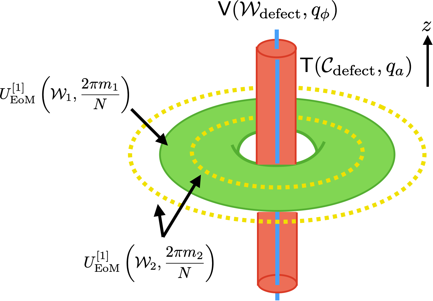
Figure 6: Anomalous Hall effect in 6d.

Here, $(r,\vartheta)$ is the polar coordinates of the 2-dimensional plane transverse to the $z$-direction. ${\mathcal{W}}_{2}$ is depicted as concentric circles that sandwich ${\mathcal{W}}_{1}$.

With this setup, the phase factor appearing in the RHS of (3.42) is identified with a magnetic flux along the $\vartheta$-direction that is measured by $U_{\rm EoM}^{[1]}\left({\mathcal{W}}_{2},\frac{2\pi m}{N}\right)$. The magnetic flux is interpreted to emanate from an electric current induced along the $\alpha$-cycle of the 2-torus ${\mathcal{W}}_{1}$. This is a manifestation of the anomalous Hall effect in 6 dimensions. In fact, we note that $U_{\rm EoM}^{[1]}\left({\mathcal{W}}_{1},\frac{2\pi m}{N}\right)$ is realized by turning on a background electric field along the normal direction to ${\mathcal{W}}_{1}$, which is perpendicular to that of the induced current.

As found in [53, 54], the correlation function (3.41) is regarded as the Peiffer lifting of a 3-group. This implies that the 6d axion electrodynamics possesses the 3-group structure as in $d=4$. In the next subsubsection, we make a further computation of correlation functions to gain a stringent support that the 6d axion electrodynamics encodes a higher-group structure with the 3-group realized as a substructure.

3.2.2 Correlation functions of symmetry generators of higher ranks

Here, we discuss correlation functions involving the symmetry generators that are absent for $d=4$.

We first turn on $A_{1}=\frac{2\pi n}{N}\delta_{1}({\mathcal{V}}),~{}C_{3}=\alpha\delta_{3}({\mathcal{C}})$, which leads to the correlation function

$$\left\langle U_{\rm EoM}^{[0]}\left({\mathcal{V}},\frac{2\pi n}{N}\right)U_{\rm CW}^{[2]}\left({\mathcal{C}},\alpha\right)\right\rangle.$$ (3.43)

By gauging away $A_{1}$ and using the GS transformation law (3.10), we find

$$\left\langle U_{\rm EoM}^{[0]}\left({\mathcal{V}},\frac{2\pi n}{N}\right)U_{\rm CW}^{[2]}\left({\mathcal{C}},\alpha\right)\right\rangle=\left\langle U_{\rm CW}^{[2]}\left({\mathcal{C}},\alpha\right)U_{\rm CW}^{[3]}\left({\mathcal{V}}\cap{\mathcal{C}},\frac{\alpha n}{N}\right)\right\rangle\ .$$ (3.44)

As another example where the action of a symmetry generator of a lower rank gives rise to $U^{[3]}_{\rm CW}$, we find

$$\left\langle U_{\rm EoM}^{[1]}\left({\mathcal{W}},\frac{2\pi m}{N}\right)U_{\rm CW}^{[1]}\left({\mathcal{W}}^{\rm CW},\beta\right)\right\rangle=\left\langle U_{\rm CW}^{[1]}\left({\mathcal{W}}^{\rm CW},\beta\right)U_{\rm CW}^{[3]}\left({\mathcal{W}}\cap{\mathcal{W}}^{\rm CW},\frac{\beta m}{N}\right)\right\rangle\ .$$ (3.45)

Here, the LHS is defined by the partition function in the presence of $B_{2}=\frac{2\pi m}{N}\delta_{1}({\mathcal{W}}),\,B_{2}^{\rm CW}=\beta\delta_{1}({\mathcal{W}}^{\rm CW})$, while the RHS is obtained by gauging away $B_{2}$.

It is verified that the action of $U_{\rm EoM}^{[1]}$ on $U^{[2]}_{\rm CW}$ gives rise to the 4-form symmetry generator:

$$\left\langle U_{\rm EoM}^{[1]}\left({\mathcal{W}},\frac{2\pi m}{N}\right)U_{\rm CW}^{[2]}\left({\mathcal{C}},\gamma\right)\right\rangle=\left\langle U_{\rm CW}^{[2]}\left({\mathcal{C}},\gamma\right)U_{\rm CW}^{[4]}\left({\mathcal{W}}\cap{\mathcal{C}},\frac{\gamma n}{N}\right)\right\rangle\ .$$ (3.46)

We next discuss correlation functions of three symmetry generators of lower ranks. As a first example, we turn on $A_{1}=\frac{2\pi n}{N}\delta_{1}({\mathcal{V}}),\,B_{2}=\frac{2\pi m_{1}}{N}\delta_{2}({\mathcal{W}}_{1})+\frac{2\pi m_{2}}{N}\delta_{2}({\mathcal{W}}_{2})$ to define the 3-point function of $U_{\rm EoM}^{[0]}$ and $U_{\rm EoM}^{[1]}$. By gauging away both $A_{1}$ and $B_{2}$, the 3-point function becomes a correlation function involving $U_{\rm CW}^{[3]}$:

$$\Big{\langle}U_{\rm EoM}^{[0]}({\mathcal{V}},\frac{2\pi n}{N})\,U_{\rm EoM}^{[1]}({\mathcal{W}}_{1},\frac{2\pi m_{1}}{N})\,U_{\rm EoM}^{[1]}({\mathcal{W}}_{2},\frac{2\pi m_{2}}{N})\Big{\rangle}$$

$$=\Big{\langle}U_{\rm CW}^{[1]}({\mathcal{V}}\cap\Omega_{{\mathcal{W}}_{1}},\frac{2\pi nm_{1}}{N})\,U_{\rm CW}^{[1]}({\mathcal{V}}\cap\Omega_{{\mathcal{W}}_{2}},-\frac{2\pi nm_{2}}{N})$$

$$~{}~{}\times U_{\rm CW}^{[2]}({\mathcal{W}}_{1}\cap\Omega_{{\mathcal{W}}_{2}},-\frac{2\pi m_{1}m_{2}}{N})\,U_{\rm CW}^{[3]}({\mathcal{W}}_{1}\cap{\mathcal{W}}_{2}\cap\Omega_{{\mathcal{V}}},-\frac{4\pi nm_{1}m_{2}}{N^{2}})\Big{\rangle}\ .$$ (3.47)

Furthermore, turning on $B_{2}=\frac{2\pi m_{1}}{N}\delta_{2}({\mathcal{W}}_{1})+\frac{2\pi m_{2}}{N}\delta_{2}({\mathcal{W}}_{2})+\frac{2\pi m_{3}}{N}\delta_{2}({\mathcal{W}}_{3})$ and then gauging it away gives a correlation function involving $U_{\rm CW}^{[4]}$:

$$\Big{\langle}U_{\rm EoM}^{[1]}({\mathcal{W}}_{1},\frac{2\pi m_{1}}{N})\,U_{\rm EoM}^{[1]}({\mathcal{W}}_{2},\frac{2\pi m_{2}}{N})\,U_{\rm EoM}^{[1]}({\mathcal{W}}_{3},\frac{2\pi m_{3}}{N})\Big{\rangle}$$

$$=\Big{\langle}U_{\rm CW}^{[2]}({\mathcal{W}}_{1}\cap\Omega_{{\mathcal{W}}_{2}},-\frac{2\pi m_{1}m_{2}}{N})\,U_{\rm CW}^{[2]}({\mathcal{W}}_{2}\cap\Omega_{{\mathcal{W}}_{3}},-\frac{2\pi m_{2}m_{3}}{N})\,U_{\rm CW}^{[2]}({\mathcal{W}}_{3}\cap\Omega_{{\mathcal{W}}_{1}},-\frac{2\pi m_{3}m_{1}}{N})$$

$$~{}~{}\times U_{\rm CW}^{[4]}({\mathcal{W}}_{1}\cap{\mathcal{W}}_{2}\cap\Omega_{{\mathcal{W}}_{3}},-\frac{4\pi m_{1}m_{2}m_{3}}{N^{2}})\Big{\rangle}\ .$$ (3.48)

These results are regarded as a manifestation of the algebraic structures that are peculiar to the 6d axion-Maxwell theory. In particular, it follows from the last two computations that the higher-group structure in this theory should be equipped with a trinary operation among three symmetry generators.

4 Conclusion and Discussion

In this paper, we discuss higher-dimensional axion electrodynamics for the purpose of exploring a higher-group structure encoded in it by generalizing the results in [53, 54].

We first discuss how the operator-valued ambiguities that arise from gauging EoM-based global symmetries are canceled. This is achieved by gauging $(2n-2)$ Chern-Weil symmetries simultaneously. It is crucial that the CW gauge fields make a Green-Schwarz transformation under the EoM-based symmetry transformation in order to guarantee gauge invariance of the resultant theory.

The main focus of this paper is on the 6d axion-Maxwell system. We give the explicit form of the GS transformation of the four CW gauge fields. We also determine the ’t Hooft anomaly due to an ambiguity of how to extend the system to a 7d spacetime. We next compute correlation functions of the symmetry generators by employing the fact that any configuration of the symmetry generators and charged operators is constructed by turning on the background gauge fields appropriately. The correlation functions of two configurations are equal to each other up to a ’t Hooft anomaly if they are mapped to each another by a gauge transformation. On top of correlation functions that have been obtained already in [53, 54], we work out a new class of correlation functions that are peculiar to the $d=6$ case. These results suggest that the 6d axion-Maxwell system possesses a higher-group structure such that the 3-group structure found in the 4d axion-Maxwell system is encoded as a substructure. Furthermore, it is natural to expect that the possible higher-group structure should admit a trinary operation, an algebraic structure involving three symmetry generators, as discussed in section 3.2.2.

More generally, the axion-Maxwell system in $d=2n$ dimensions is expected to possess a higher-group structure with a substructure identical to that of the $d=2n-2$ axion-Maxwell system. This is because all the CW gauge field strengths for the $d=2n-2$ case are included in those for the $d=2n$ case. Furthermore, the higher-group structure for the $d=2n$ case, if exists, should admit an $n$-ary operation among $n$ symmetry generators. To see this, we note that the $d=2n$ axion-Maxwell system has the $(2n-2)$-form symmetry with the CW current $d\phi/(2\pi)$, and it couples to a $(2n-1)$-form CW gauge field. The gauge invariant $2n$-form field strength contains a term proportional to $(B_{2})^{n}$. This implies that two correlation functions, one with a single insertion of the symmetry generator $U_{\rm CW}^{[2n-2]}$ and the other with $n$ insertions of $U_{\rm EoM}^{[1]}$, are related with each other as found in (3.48) for $n=3$.

In this paper, we have not attempted to formulate rigorously the mathematical structure of the higher-group symmetry that underlies the higher-dimensional axion-Maxwell systems. We leave it for future work.

Acknowledgements

RY is supported by JSPS KAKENHI Grants No. JP21J00480, JP21K13928.

Appendix A Alternative method of computing correlation functions

In section 3.2, correlation functions are computed using a network of background gauge fields and gauge transformations acting on it. Here, we review an alternative way that is developed in [53] for the 4d axion-Maxwell system.

Let $S[\phi,a]$ be the action (2.1). Shifting the axion and the Maxwell field by the background gauge fields $\Phi_{0}$ and $\Pi_{1}$, respectively, we find

$$S[\phi,a]+\int_{{\mathcal{M}}_{2n}}dj^{[0]}_{\rm EoM}\wedge\Phi_{0} =S[\phi-\Phi_{0},a]+\frac{1}{2}\int_{{\mathcal{M}}_{2n}}d\Phi_{0}\wedge\star d\Phi_{0}\ ,$$ (A.1)

$$S[\phi,a]+\int_{{\mathcal{M}}_{2n}}dj^{[1]}_{\rm EoM}\wedge\Pi_{1} =S[\phi,a+\Pi_{1}]+\frac{N}{(2\pi)^{n}}\sum_{r=2}^{n}\frac{1}{(n-r)!r!}d\phi(da)^{n-r}\wedge(d\Pi_{1})^{r-1}\wedge\Pi_{1}$$

$$~{}~{}~{}+\frac{1}{2}\int_{{\mathcal{M}}_{2n}}d\Pi_{1}\wedge\star d\Pi_{1}\ .$$ (A.2)

These results play a key role in the computations made below.

As a sample computation, we discuss the correlation function of $U_{\rm EoM}^{[0]}({\mathcal{V}},\frac{2\pi n}{N})$ and $U_{\rm CW}^{[1]}({\mathcal{W}},\frac{2\pi m}{N})$ for the $n=3$ case. Noting that $U_{\rm EoM}^{[0]}({\mathcal{V}},\frac{2\pi n}{N})$ is rewritten as

$$U_{\rm EoM}^{[0]}({\mathcal{V}},\frac{2\pi n}{N})=\exp(\frac{2\pi}{N}\int_{\mathcal{V}}j_{\rm EoM}^{[0]})=\exp(\frac{2\pi}{N}\int_{{\mathcal{M}}_{6}}dj_{\rm EoM}^{[0]}\wedge\delta_{0}(\Omega_{\mathcal{V}}))\ ,$$ (A.3)

it follows from (A.1) with $\Phi_{0}=(2\pi/N)\,\delta_{0}(\Omega_{\mathcal{V}})$ that

$$\left\langle U_{\rm EoM}^{[0]}\left({\mathcal{V}},\frac{2\pi n}{N}\right)U_{\rm EoM}^{[1]}\left({\mathcal{W}},\frac{2\pi m}{N}\right)\right\rangle={\cal N}\int{\cal D}[\phi,a]e^{iS[\phi-\frac{2\pi n}{N}\delta_{0}(\Omega_{\mathcal{V}}),a]+\frac{2\pi im}{N}\int_{\mathcal{W}}j^{[1]}_{\rm EoM}}\ .$$ (A.4)

By shifting $\phi\rightarrow\phi^{\prime}=\phi-\frac{2\pi n}{N}\delta_{0}(\Omega_{\mathcal{V}})$, we obtain

$$\left\langle U_{\rm EoM}^{[0]}\left({\mathcal{V}},\frac{2\pi n}{N}\right)U_{\rm EoM}^{[1]}\left({\mathcal{W}},\frac{2\pi m}{N}\right)\right\rangle= {\cal N}\int{\cal D}[\phi^{\prime},a]e^{iS[\phi^{\prime},a]+\frac{2\pi im}{N}\int_{\mathcal{W}}j^{[1]}_{\rm EoM}-\frac{inm}{4\pi N}\int_{\mathcal{W}}da\wedge da\delta_{0}(\Omega_{\mathcal{V}})}$$

$$= \left\langle U_{\rm EoM}^{[1]}\left({\mathcal{W}},\frac{2\pi m}{N}\right)U_{\rm CW}^{[1]}\left({\mathcal{W}}\cap\Omega_{\mathcal{V}},-\frac{2\pi nm}{N}\right)\right\rangle\ ,$$ (A.5)

because $j_{\rm EoM}^{[1]}$ gets shifted under the shift. This coincides with (3.39).

The rest of the correlations computed in this paper can be reproduced following the the same way as discussed in this appendix.

References

- [1] D. Gaiotto, A. Kapustin, N. Seiberg and B. Willett, Generalized Global Symmetries, JHEP 02 (2015) 172 [1412.5148].
- [2] C.D. Batista and Z. Nussinov, Generalized Elitzur’s theorem and dimensional reduction, Phys. Rev. B 72 (2005) 045137 [cond-mat/0410599].
- [3] T. Pantev and E. Sharpe, GLSM’s for Gerbes (and other toric stacks), Adv. Theor. Math. Phys. 10 (2006) 77 [hep-th/0502053].
- [4] T. Pantev and E. Sharpe, String compactifications on Calabi-Yau stacks, Nucl. Phys. B 733 (2006) 233 [hep-th/0502044].
- [5] Z. Nussinov and G. Ortiz, Sufficient symmetry conditions for Topological Quantum Order, Proc. Nat. Acad. Sci. 106 (2009) 16944 [cond-mat/0605316].
- [6] Z. Nussinov and G. Ortiz, Autocorrelations and thermal fragility of anyonic loops in topologically quantum ordered systems, Phys. Rev. B 77 (2008) 064302 [0709.2717].
- [7] Z. Nussinov and G. Ortiz, A symmetry principle for topological quantum order, Annals Phys. 324 (2009) 977 [cond-mat/0702377].
- [8] Z. Nussinov, G. Ortiz and E. Cobanera, Effective and exact holographies from symmetries and dualities, Annals Phys. 327 (2012) 2491 [1110.2179].
- [9] T. Banks and N. Seiberg, Symmetries and Strings in Field Theory and Gravity, Phys. Rev. D 83 (2011) 084019 [1011.5120].
- [10] J. Distler and E. Sharpe, Quantization of Fayet-Iliopoulos Parameters in Supergravity, Phys. Rev. D 83 (2011) 085010 [1008.0419].
- [11] A. Kapustin and R. Thorngren, Higher symmetry and gapped phases of gauge theories, 1309.4721.
- [12] A. Kapustin and N. Seiberg, Coupling a QFT to a TQFT and Duality, JHEP 04 (2014) 001 [1401.0740].
- [13] D. Gaiotto, A. Kapustin, Z. Komargodski and N. Seiberg, Theta, Time Reversal, and Temperature, JHEP 05 (2017) 091 [1703.00501].
- [14] D. Gaiotto, Z. Komargodski and N. Seiberg, Time-reversal breaking in QCD4, walls, and dualities in 2 + 1 dimensions, JHEP 01 (2018) 110 [1708.06806].
- [15] Y. Tanizaki, T. Misumi and N. Sakai, Circle compactification and ’t Hooft anomaly, JHEP 12 (2017) 056 [1710.08923].
- [16] Y. Tanizaki, Y. Kikuchi, T. Misumi and N. Sakai, Anomaly matching for the phase diagram of massless -QCD, Phys. Rev. D 97 (2018) 054012 [1711.10487].
- [17] Z. Komargodski, A. Sharon, R. Thorngren and X. Zhou, Comments on Abelian Higgs Models and Persistent Order, SciPost Phys. 6 (2019) 003 [1705.04786].
- [18] Y. Hirono and Y. Tanizaki, Quark-Hadron Continuity beyond the Ginzburg-Landau Paradigm, Phys. Rev. Lett. 122 (2019) 212001 [1811.10608].
- [19] Y. Hirono and Y. Tanizaki, Effective gauge theories of superfluidity with topological order, JHEP 07 (2019) 062 [1904.08570].
- [20] Y. Hidaka, Y. Hirono, M. Nitta, Y. Tanizaki and R. Yokokura, Topological order in the color-flavor locked phase of a (3+1)-dimensional U(N) gauge-Higgs system, Phys. Rev. D 100 (2019) 125016 [1903.06389].
- [21] M.M. Anber and E. Poppitz, On the baryon-color-flavor (BCF) anomaly in vector-like theories, JHEP 11 (2019) 063 [1909.09027].
- [22] T. Misumi, Y. Tanizaki and M. Ünsal, Fractional angle, ’t Hooft anomaly, and quantum instantons in charge- multi-flavor Schwinger model, JHEP 07 (2019) 018 [1905.05781].
- [23] M.M. Anber and E. Poppitz, Deconfinement on axion domain walls, JHEP 03 (2020) 124 [2001.03631].
- [24] M.M. Anber and E. Poppitz, Generalized ’t Hooft anomalies on non-spin manifolds, JHEP 04 (2020) 097 [2002.02037].
- [25] Y. Hidaka, Y. Hirono and R. Yokokura, Counting Nambu-Goldstone Modes of Higher-Form Global Symmetries, Phys. Rev. Lett. 126 (2021) 071601 [2007.15901].
- [26] N. Yamamoto and R. Yokokura, Topological mass generation in gapless systems, Phys. Rev. D 104 (2021) 025010 [2009.07621].
- [27] T. Furusawa and M. Hongo, Global anomaly matching in the higher-dimensional model, Phys. Rev. B 101 (2020) 155113 [2001.07373].
- [28] N. Yamamoto and R. Yokokura, Unstable Nambu-Goldstone modes, Phys. Rev. D 106 (2022) 105004 [2203.02727].
- [29] J.C. Baez and A.D. Lauda, Higher-dimensional algebra v: 2-groups, Theory and Applications of Categories 12 (2004) 423 [math/0307200].
- [30] A. Kapustin and R. Thorngren, Topological Field Theory on a Lattice, Discrete Theta-Angles and Confinement, Adv. Theor. Math. Phys. 18 (2014) 1233 [1308.2926].
- [31] E. Sharpe, Notes on generalized global symmetries in QFT, Fortsch. Phys. 63 (2015) 659 [1508.04770].
- [32] L. Bhardwaj, D. Gaiotto and A. Kapustin, State sum constructions of spin-TFTs and string net constructions of fermionic phases of matter, JHEP 04 (2017) 096 [1605.01640].
- [33] A. Kapustin and R. Thorngren, Fermionic SPT phases in higher dimensions and bosonization, JHEP 10 (2017) 080 [1701.08264].
- [34] Y. Tachikawa, On gauging finite subgroups, SciPost Phys. 8 (2020) 015 [1712.09542].
- [35] R.C. de Almeida, J.P. Ibieta-Jimenez, J.L. Espiro and P. Teotonio-Sobrinho, Topological Order from a Cohomological and Higher Gauge Theory perspective, 1711.04186.
- [36] F. Benini, C. Córdova and P.-S. Hsin, On 2-Group Global Symmetries and their Anomalies, JHEP 03 (2019) 118 [1803.09336].
- [37] C. Córdova, T.T. Dumitrescu and K. Intriligator, Exploring 2-Group Global Symmetries, JHEP 02 (2019) 184 [1802.04790].
- [38] C. Delcamp and A. Tiwari, From gauge to higher gauge models of topological phases, JHEP 10 (2018) 049 [1802.10104].
- [39] X.-G. Wen, Emergent anomalous higher symmetries from topological order and from dynamical electromagnetic field in condensed matter systems, Phys. Rev. B 99 (2019) 205139 [1812.02517].
- [40] C. Delcamp and A. Tiwari, On 2-form gauge models of topological phases, JHEP 05 (2019) 064 [1901.02249].
- [41] R. Thorngren, Topological quantum field theory, symmetry breaking, and finite gauge theory in 3+1D, Phys. Rev. B 101 (2020) 245160 [2001.11938].
- [42] C. Cordova, T.T. Dumitrescu and K. Intriligator, 2-Group Global Symmetries and Anomalies in Six-Dimensional Quantum Field Theories, JHEP 04 (2021) 252 [2009.00138].
- [43] P.-S. Hsin and A. Turzillo, Symmetry-enriched quantum spin liquids in (3 + 1), JHEP 09 (2020) 022 [1904.11550].
- [44] P.-S. Hsin and H.T. Lam, Discrete theta angles, symmetries and anomalies, SciPost Phys. 10 (2021) 032 [2007.05915].
- [45] S. Gukov, P.-S. Hsin and D. Pei, Generalized global symmetries of theories. Part I, JHEP 04 (2021) 232 [2010.15890].
- [46] N. Iqbal and N. Poovuttikul, 2-group global symmetries, hydrodynamics and holography, 2010.00320.
- [47] T. Brauner, Field theories with higher-group symmetry from composite currents, JHEP 04 (2021) 045 [2012.00051].
- [48] O. DeWolfe and K. Higginbotham, Generalized symmetries and 2-groups via electromagnetic duality in , Phys. Rev. D 103 (2021) 026011 [2010.06594].
- [49] B. Heidenreich, J. McNamara, M. Montero, M. Reece, T. Rudelius and I. Valenzuela, Chern-Weil global symmetries and how quantum gravity avoids them, JHEP 11 (2021) 053 [2012.00009].
- [50] F. Apruzzi, S. Schafer-Nameki, L. Bhardwaj and J. Oh, The Global Form of Flavor Symmetries and 2-Group Symmetries in 5d SCFTs, SciPost Phys. 13 (2022) 024 [2105.08724].
- [51] L. Bhardwaj, 2-Group symmetries in class S, SciPost Phys. 12 (2022) 152 [2107.06816].
- [52] J.C. Baez and J. Huerta, An Invitation to Higher Gauge Theory, Gen. Rel. Grav. 43 (2011) 2335 [1003.4485].
- [53] Y. Hidaka, M. Nitta and R. Yokokura, Higher-form symmetries and 3-group in axion electrodynamics, Phys. Lett. B 808 (2020) 135672 [2006.12532].
- [54] Y. Hidaka, M. Nitta and R. Yokokura, Global 3-group symmetry and ’t Hooft anomalies in axion electrodynamics, JHEP 01 (2021) 173 [2009.14368].
- [55] Y. Hidaka, M. Nitta and R. Yokokura, Global 4-group symmetry and ’t Hooft anomalies in topological axion electrodynamics, PTEP 2022 (2022) 04A109 [2108.12564].
- [56] T.D. Brennan and C. Cordova, Axions, higher-groups, and emergent symmetry, JHEP 02 (2022) 145 [2011.09600].
- [57] E. Witten, Dyons of Charge e theta/2 pi, Phys. Lett. B 86 (1979) 283.
- [58] P. Sikivie, On the Interaction of Magnetic Monopoles With Axionic Domain Walls, Phys. Lett. B 137 (1984) 353.
- [59] X.-L. Qi, T. Hughes and S.-C. Zhang, Topological Field Theory of Time-Reversal Invariant Insulators, Phys. Rev. B 78 (2008) 195424 [0802.3537].
- [60] J.C.Y. Teo and C.L. Kane, Topological Defects and Gapless Modes in Insulators and Superconductors, Phys. Rev. B 82 (2010) 115120 [1006.0690].
- [61] Z. Wang and S.-C. Zhang, Chiral anomaly, charge density waves, and axion strings from Weyl semimetals, Phys. Rev. B 87 (2013) 161107 [1207.5234].
- [62] M.B. Green and J.H. Schwarz, Anomaly Cancellation in Supersymmetric D=10 Gauge Theory and Superstring Theory, Phys. Lett. B 149 (1984) 117.