End-to-End Stochastic Optimization with Energy-Based Model

Abstract

Decision-focused learning (DFL) was recently proposed for stochastic optimization problems that involve unknown parameters. By integrating predictive modeling with an implicitly differentiable optimization layer, DFL has shown superior performance to the standard two-stage predict-then-optimize pipeline. However, most existing DFL methods are only applicable to convex problems or a subset of nonconvex problems that can be easily relaxed to convex ones. Further, they can be inefficient in training due to the requirement of solving and differentiating through the optimization problem in every training iteration. We propose So-Ebm, a general and efficient DFL method for stochastic optimization using energy-based models. Instead of relying on KKT conditions to induce an implicit optimization layer, So-Ebm explicitly parameterizes the original optimization problem using a differentiable optimization layer based on energy functions. To better approximate the optimization landscape, we propose a coupled training objective that uses a maximum likelihood loss to capture the optimum location and a distribution-based regularizer to capture the overall energy landscape. Finally, we propose an efficient training procedure for So-Ebm with a self-normalized importance sampler based on a Gaussian mixture proposal. We evaluate So-Ebm in three applications: power scheduling, COVID-19 resource allocation, and non-convex adversarial security game, demonstrating the effectiveness and efficiency of So-Ebm.

1 Introduction

Many real-life decision making tasks are stochastic optimization problems, where one needs to make decisions to minimize a cost function that involves stochastic parameters. Oftentimes, the involved stochastic parameters are unknown and context-dependent, meaning that they need to be predicted from observed features. For example, when allocating clinical resources for COVID-19, it is necessary to consider future cases in different regions, whose distributions are unknown and have to be predicted from the current state. As two other examples, hedge funds need to continuously adjust their portfolio for maximal expected return, by forecasting future return rates of different stocks; and in supply chain optimization, facility locations need to be decided to minimize long-term operational costs, by accounting for unknown and uncertain regional supplies and customer demands.

With the feasibility of training powerful deep learning predictors from large amounts of data, it is increasingly common to solve such stochastic optimization problems using a two-stage predict-then-optimize pipeline. In the prediction stage, one learns a predictive model for the unknown parameters using certain prediction loss (e.g., negative likelihood). In the optimization stage, the predicted distributions of the parameters are used to parameterize the stochastic optimization problem, which can be then solved using off-the-shelf solvers hart2011pyomo ; agrawal2018rewriting ; diamond2016cvxpy . This two-stage pipeline relies on an implicit and commonly-accepted assumption: improvements in parameter prediction in terms of the prediction loss will always translate to better optimization outcomes. However, this is not the case: machine learning models make errors and the impact of prediction errors is not uniform w.r.t. the optimization loss. Thus, a smaller predictive loss does not necessarily lead to a smaller decision regret.

A better approach is decision-focused learning (DFL) donti2017task ; agrawal2019differentiable ; amos2017optnet , which integrates prediction and optimization layers into a unified model to learn them end-to-end. Most DFL methods implement the optimization procedure as an implicitly differentiable layer and develop techniques (e.g., using KKT conditions) to compute the gradients w.r.t. the decision variables and enable back-propagating through it. Compared to the two-stage pipeline, the prediction layer so learned is tailored for the optimization problem and better in the sense that it can yield decisions with smaller regrets. Besides DFL, there are also approaches where a policy network is trained to directly map from the input to the solution of the optimization problem using supervised or reinforcement learning vinyals2015pointer ; khalil2017learning ; li2016learning . However, their performance are often inferior to DFL as they ignore the algorithmic structure of the problem and typically require a large amount of data to rediscover the algorithmic structure.

Despite their promising results, existing DFL methods donti2017task ; amos2017optnet ; agrawal2019differentiable ; perrault2019decision ; wang2020scalable suffer from two drawbacks. (1) Generality. To leverage the KKT condition, they are mostly applicable to only convex optimization objectives donti2017task ; amos2017optnet ; agrawal2019differentiable . Though a few works approximate nonconvex objectives by quadratic functions perrault2019decision ; wang2020scalable , their applicability is still limited to easy-to-relax nonconvex problems and can suffer from poor gradient estimates caused by the relaxation. (2) Scalability. Due to the reliance of using the KKT condition to compute derivatives, they require repeatedly solving the optimization program and back-propagating through it during training, which makes them unscalable. The problem is more severe when the expectation of the cost cannot be computed analytically.

We propose a new end-to-end stochastic optimization method using an energy-based model (EBM), named So-Ebm. Similar to DFL, So-Ebm models the algorithmic predict-and-optimize structure by stacking a differentiable optimization layer on top of a neural predictor. Different from DFL, So-Ebm eliminates the need of using KKT conditions to induce an implicit differentiable optimization layer. Instead, it leverages expressive EBMs lecun2006tutorial to directly model the conditional probability of the decisions and parameterizes an explicit energy-based differentiable layer as a surrogate to the original optimization problem. To better approximate the optimization landscape with the EBM surrogate, we design two complementary learning objectives in So-Ebm: 1) a local matching objective that maximizes the likelihood of the optimal decisions; and 2) a global matching objective that minimizes the distribution distance between the posterior distribution of the decision variables and the surrogate-based decision distribution.

Due to its flexibility, So-Ebm is not constrained to convex objectives, but can be applied to a wide class of stochastic optimization problems. Another key advantage of So-Ebm is its computational efficiency. As the optimization layer is parameterized by an energy-based model, So-Ebm eliminates the need of solving and differentiating through the optimization procedure at each training iteration. Rather, So-Ebm estimates the derivatives of the energy-based surrogate model using a self-normalized importance sampler. We design a Gaussian-mixture proposal distribution for the sampler, which not only reduces sampling variance, but also borrows the idea of contrastive divergence for MCMC methods to speed up the training of So-Ebm.

The main contributions of this work are: (1) We propose a new end-to-end stochastic optimization method based on energy-based model. It avoids the needs of solving and differentiating through the optimization problem during training and can be applied to a wide range of stochastic optimization problems beyond convex objectives. (2) We propose a coupled training objective to encourage the energy-based surrogate to well approximate the optimization landscape and an efficient self-normalized importance sampler based on a mixture-of-Gaussian proposal. (3) Experiments on power scheduling, COVID-19 resource allocation and adversarial network security game show that our method can achieve better or comparable performance than existing DFL methods while being much more efficient.

2 Preliminaries

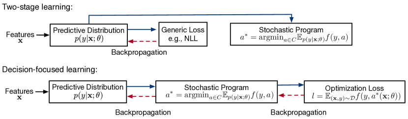
Figure 1: Two-stage learning back-propagates from a predictive loss to the model, ignoring the latter effect of the optimization problem. Decision-focused learning directly optimizes the task loss but needs to solve and back-propagate through the optimization problem at every training iteration.

Problem Formulation. Consider a stochastic optimization problem:

$$\operatorname{arg\,min}_{a\in C}f(y,a),$$

where $y$ denotes the parameters of the optimization problem, $a$ denotes the decision variables within a feasible space $C$, and $f$ is the cost function to be optimized. In many applications, the parameters $y$ are unknown and stochastic, which must be inferred from some correlated features $\mathbf{x}$. We assume a dataset $\mathcal{D}=\{\mathbf{x}_{i},y_{i}\}_{i=1}^{N}$ drawn from the joint distribution of the features and problem parameters. Our task is to learn a decision-making model $\mathbf{M}$ parameterized by $\theta$, which takes the features $\mathbf{x}$ as input and outputs the optimal decisions $a^{*}(\mathbf{x};\theta)$. The model should be learned such that its output optimal decisions minimize the expected decision cost under the joint distribution of $(\mathbf{x},y)$, namely:

$$\operatorname{arg\,min}_{\theta}\mathbb{E}_{(\mathbf{x},y)\sim\mathcal{D}}f(y,a^{*}(\mathbf{x};\theta)).$$

For example, in supply chain optimization, $y$ can be regional customer demands, $a$ can be pre-ordered products for each region, $f$ measures the gap between actual customer demands and pre-ordered supplies, and the problem is to decide the best $a$ to minimize the cost $f$. Herein, the actual customer demands $y$ are usually unknown and must be predicted from features $\mathbf{x}$ such as customer purchase history and regional economy indices.

Two-stage learning v.s. Decision Focused Learning (DFL). A common practice to the above stochastic optimization problem is the two-stage predict-then-optimize framework. It first learns an probabilistic predictive model $p(y|\mathbf{x};\theta)$ and then uses existing stochastic optimization solvers to obtain the optimal action that minimizes the expected cost: $a^{*}(\mathbf{x};\theta)=\operatorname{arg\,min}_{a\in C}\mathbb{E}_{y\sim p(y|\mathbf{x};\theta)}f(y,a)$. Though the two-stage approach is simple and efficient, it can suffer from suboptimal performance due to the misalignment of the prediction loss and the optimization loss. In contrast, DFL integrates prediction and optimization into an end-to-end model, thus tailoring the predictive model for the optimization task, as shown in Figure 1. By directly optimizing the task loss, the gradient of the model parameters can be obtained with the following chain rule:

$$\frac{\partial f(y,a^{*}(\mathbf{x};\theta))}{\partial\theta}=\frac{\partial f(y,a^{*}(\mathbf{x};\theta))}{\partial a^{*}(\mathbf{x};\theta)}\frac{\partial{a^{*}(\mathbf{x};\theta)}}{\partial{y}}\frac{\partial y}{\partial{\theta}}.$$

The key challenge here is to compute the Jacobian $\frac{\partial{a^{*}(\mathbf{x};\theta)}}{\partial y}$: it is needed to apply the chain rule to learn the model using gradient decent methods. This is nontrivial, because $a^{*}$ is the solution of a stochastic optimization solver and not directly differentiable. To address this challenge, OptNet donti2017task ; amos2017optnet assumes quadratic optimization objectives and differentiates through the KKT conditions using the implicit function theorem. This way, OptNet can obtain the Jacobian by solving the optimization problem along with a set of linear equations in each training iteration. Several works agrawal2019differentiable ; perrault2019decision ; wang2020scalable extend this technique to more general cases. For example, cvxpylayers agrawal2019differentiable extends it to more general cases of convex optimization using disciplined parametrized programming (DPP) grammar.

Although existing DFL approaches can achieve better decisions compared to two-stage learning, they have several drawbacks. First, they are often constrained to convex optimization objectives as they rely on the KKT conditions to compute derivatives. Though perrault2019decision ; wang2020scalable propose to approximate some non-convex objectives by a quadratic function around a local minimum, the inaccurate gradients may be aggregated during the training iterations and thus lead to poor decision quality. Second, they suffer from high computational complexity because the computation of the Jacobian $\frac{\partial{a^{*}(\mathbf{x};\theta)}}{\partial y}$ requires repeatedly solving the optimization program and back-propagating through it. The problem is more severe when the expectation of the cost cannot be computed analytically. In that case, we need to use sample average approximation kim2015guide ; verweij2003sample ; kleywegt2002sample and draw multiple IID samples from the predictive distribution, which makes the objective much more complicated and expensive.

3 Proposed Method

3.1 Energy-based Model for End-to-end Stochastic Programming

Our task is to learn an optimal decision-making model $\mathbf{M}_{\theta}$, such that its output optimal decision $a^{*}(\mathbf{x};\theta)$ for input $\mathbf{x}$ minimizes the expected optimization cost: $\mathbb{E}_{(\mathbf{x},y)\sim\mathcal{D}}f(y,a^{*}(\mathbf{x};\theta))$. The core idea of our method is to directly model $\mathbf{M}_{\theta}$’s probability distribution over the decisions conditioned on the features, denoted as $q(a|\mathbf{x};\theta)$, using energy-based parameterization lecun2006tutorial :

$$q(a|\mathbf{x};\theta)=\frac{\text{exp}(-E(\mathbf{x},a;\theta))}{Z(\mathbf{x},\theta)},\quad Z(\mathbf{x};\theta)=\int\text{exp}(-E(\mathbf{x},a;\theta)da.$$ (1)

To parameterize the energy function $E(\mathbf{x},a;\theta)$, a natural option is to directly use a deep neural network which takes a feature-decision pair $(\mathbf{x},a)$ as input and output a scalar value. However, such a design ignores the algorithmic structure of the optimization problem and thus can be data-inefficient during learning. Instead, we propose to explicitly model the problem structure by using the expected task loss as the energy function:

$$E(\mathbf{x},a;\theta)=\mathbb{E}_{p(y|\mathbf{x};\theta)}f(y,a),$$ (2)

where $p(y|\mathbf{x};\theta)$ is the predictive distribution of an uncertainty-aware neural network gal2016dropout ; kong2020sde .

Eq. 2 creates an explicit energy-based differentiable layer as a surrogate to the original optimization problem. Compared with the two-stage model, it builds a direct connection between the input features $\mathbf{x}$ and decision variable $a$ and thus is more tailored to the downstream task. Compared with pure end-to-end architectures, the task-based surrogate energy function explicitly leverages the algorithmic structure of the optimization problem and thus saves a lot of learning. This energy-based surrogate function also has a intuitive interpretation. When the decision $a$ is in a region with smaller expected task loss, it has lower energy and higher probability; when it leads to higher expected task loss, it has higher energy and lower probability.

Since we have the ground truth for the parameters $y$ in the training data, the feature-decision pairs $\mathcal{D}_{a}=\{(\mathbf{x}_{i},a_{i}^{*})\}_{i=1}^{N}$ can be easily constructed by solving $a^{*}_{i}=\operatorname{arg\,min}_{a_{i}\in C}f(y_{i},a_{i})$ for each $(\mathbf{x}_{i},y_{i})$ using any off-the-shelf optimization solvers. Note that the construction of such feature-action training pairs needs to be done only once during preprocessing (Fig. 3). Then, we minimize the negative log-likelihood (NLL) of all the feature-decision pairs:

$$\ell_{\text{MLE}}=-\mathbb{E}_{(\mathbf{x},a^{*})\sim\mathcal{D}_{a}}q(a^{*}|\mathbf{x};\theta)=\mathbb{E}_{(\mathbf{x},a^{*})\sim\mathcal{D}_{a}}\left(\mathbb{E}_{p(y|\mathbf{x};\theta)}f(y,a^{*})+\text{log}(Z(\mathbf{x};\theta))\right).$$ (3)

By minimizing the NLL, we are essentially minimizing the energy of the optimal actions while maximizing the energy of other points. Thus the end-to-end stochastic programming problem is translated to learning a neural network that outputs the smallest energy for the optimal actions. This new perspective avoids the need of solving and differentiating through the optimization problem at every training iteration, but meanwhile tailors the model for the downstream decision making task.

Our energy-based formulation can also be interpreted as a non-sequential maximum entropy inverse reinforcement learning (MaxEN-IRL) model ziebart2008maximum ; wulfmeier2015maximum . From the IRL perspective, the input features $\{\mathbf{x}_{i}\}_{i=1}^{N}$ can be interpreted as environment states, the feature-decision pairs $\{(\mathbf{x}_{i},a_{i})\}_{i=1}^{N}$ as expert demonstrations, and the negative expected task loss $-\mathbb{E}_{p(y|\mathbf{x};\theta)}f(y,a)$ as reward. Eq. 3 is then equivalent to maximizing the likelihood of the expert demonstrations (optimal decisions) to recover the hidden reward function.

3.2 Augmenting Energy-Based Objective with Distribution Regularizer

One limitation of learning with EBM-based likelihood for the optimization problem is that we model only one data point $a^{*}$ for each conditional distribution $q(a|\mathbf{x};\theta)$. Minimizing the NLL for a single data point ignores the overall matchness between the landscape of original optimization problem and that of the EBM-based probability density, which can easily cause overfitting. To learn the overall shape of the energy function better, we propose a distribution-based regularizer which augments the energy-based objective from a global training perspective.

The distribution-based regularizer is based on minimizing the distance between the model distribution and an oracle posterior distribution. Specifically, we assume that $a$ follows a prior distribution $p(a)$. With the ground-truth label $y$, the posterior distribution of $a$ is then given by $p(a|y)=\frac{p(a)\text{exp}(-f(y,a))}{Z(y)}$ when we define the task loss as the negative log-likelihood, i.e.,$-\log p(y|a)=f(y,a)$. However, such an expression depends on the ground-truth label, which cannot be obtained at test time. We let the model distribution $q(a|\mathbf{x};\theta)$ mimic this oracle posterior $p(a|y)$ distribution by minimizing their KL-divergence:

$$\ell_{\text{KL}}=\mathbb{E}_{(\mathbf{x},y)\sim\mathcal{D}}\text{KL}[p(a|y)||q(a|\mathbf{x};\theta)]\\ =\mathbb{E}_{(\mathbf{x},y)\sim\mathcal{D}}\left(-\mathbb{E}_{p(a|y)}\log q(a|\mathbf{x};\theta)-\mathcal{H}(p(a|y))\right),$$ (4)

where $\mathcal{H}(\cdot)$ denotes entropy of the probability distribution. Our final training loss is a weighted combination of the NLL and the distribution based regularizer:

$$\ell_{\text{Total}}=\ell_{\text{MLE}}+\lambda\ell_{\text{KL}},$$ (5)

where $\lambda$ is a hyper-parameter. In this final objective, the KL-divergence loss and the NLL loss complement each other (Fig. 2). The NLL loss is a local training strategy while the KL-divergence loss learns the energy function from a global level. Specifically, the NLL loss helps the model capture the location of the optimal decision better but ignores the overall energy shape. The distribution-based regularizer essentially adds more anchor points besides the optimal decisions and thus helps fit the overall energy shape.

Figure 2: Different training objectives of energy-based optimization. (a) the ground-truth energy-based landscape; (b) MLE training captures the location of the optimum but ignores the overall energy shape; (c) KL-divergence training learns the overall energy shape but captures a blurry optimum location; (d) Our MLE+KL-divergence training wins the best of both worlds.

3.3 Training with Contrastive Divergence and Self-normalized Importance Sampling

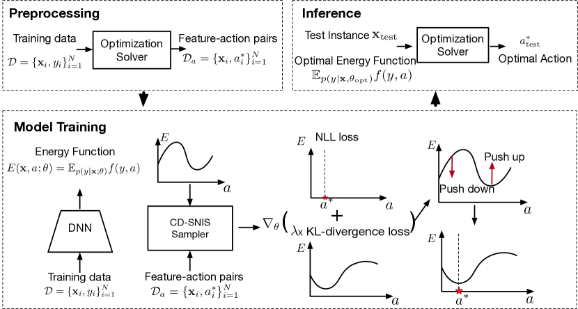
Figure 3: Illustration of So-Ebm: end-to-end stochastic optimization with energy-based model.

Optimizing Eq. 5 requires evaluating the partition function and computing the KL-divergence between two continuous distributions which typically involves intractable integrals. In this subsection, we propose to use a self-normalized importance sampler based on mixture of Gaussians to estimate the gradient of the model parameters efficiently. First, we derive (see supplementary for details) the gradient of the training loss with respect to the model parameters $\theta$ as:

$$\frac{\partial\mathcal{L}_{\text{Total}}}{\partial\theta}= \mathbb{E}_{(\mathbf{x},a^{*})\sim\mathcal{D}_{a}}\left(\frac{\partial E(a^{*},\mathbf{x};\theta)}{\partial\theta}-\mathbb{E}_{q(\tilde{a}|\mathbf{x};\theta)}\frac{\partial E(\tilde{a},\mathbf{x};\theta)}{\partial\theta}\right)$$ (6)

$$+\lambda\mathbb{E}_{(\mathbf{x},y)\sim\mathcal{D}}\left(\mathbb{E}_{p(\hat{a}|y)}\frac{\partial E(\hat{a},\mathbf{x};\theta)}{\partial\theta}-\mathbb{E}_{q(\tilde{a}|\mathbf{x};\theta)}\frac{\partial E(\tilde{a},\mathbf{x};\theta)}{\partial\theta}\right).$$

As can be seen, the gradient can be estimated by sampling from the model distribution $q(a|\mathbf{x};\theta)$ and oracle distribution $p(a|y)$. Unfortunately, we cannot easily draw samples because of the unnormalized constant. Existing methods usually resort to MCMC methods (e.g., Langevin dynamics) to use this gradient estimator. However, MCMC is an iterative process and can be time consuming. To improve the training efficiency, we propose to use a self-normalized importance sampler based on a Gaussian mixture proposal to estimate the gradient.

Specifically, for each $\mathbf{x}$, we first sample a set of $M$ candidates $\{a^{m}\}_{m=1}^{M}$ from a proposal distribution $\pi(a|\mathbf{x})$, and then sample $\tilde{a}$ from the empirical distribution located at each $a^{m}$ and weighted proportionally to $\text{exp}(-E(a|\mathbf{x};\theta))/\pi(a|\mathbf{x})$. To reduce the variance of the self-normalized importance sampler, we propose to use a mixture of $K$ Gaussians which are centered at the location of the corresponding optimal decision as the proposal distribution: $\pi(a|\mathbf{x})=\frac{1}{K}\sum_{i=1}^{K}\mathcal{N}(a^{*};\sigma_{k}),$ where $K$ and $\{\sigma_{k}\}_{k=1}^{K}$ are hyper-parameters. This mixture of Gaussian based self-normalized importance sampler enjoys great computational efficiency. We only need to estimate the gradient of the energy-based surrogate layer by drawing samples from a simple mixture of Gaussians, instead of solving and differentiating through the optimization problem as in DFL. This significantly reduces the training time compared with DFL as shown in Section 4. Further, locating the proposal distribution at the optimal decisions mimics the contrastive divergence method hinton2002training ; du2019implicit used in Langevin dynamics where the MCMC chain starts from the training data. This makes the proposal distribution close to the model distribution and thus has better sample efficiency. The sampling procedure from the oracle distribution $p(a|y)$ is similar with $q(a|\mathbf{x};\theta)$.

When the expected task loss has no analytical expression, we can draw multiple samples from $p(y|\mathbf{x};\theta)$ to estimate the expectation and use reparameterization trick kingma2013auto ; jang2016categorical ; maddison2017concrete ; rezende2014stochastic to make it differentiable. Finally, the model can be efficiently trained via gradient-based method, such as Adam kingma2015adam . The detailed training procedure is given in Alg. 1 in the supplementary.

Model inference. With the optimal model parameter $\theta_{\text{opt}}$, we draw samples from $q(a|\mathbf{x}_{\rm test};\theta_{\text{opt}})$ for an unseen test instance $\mathbf{x}_{\rm test}$. However, in the real-world applications, we usually only need the most optimal decision. This can be obtained by solving $\operatorname{arg\,min}_{a^{*}_{\rm test}\in C}\mathbb{E}_{p(y|\mathbf{x}_{\rm test};\theta_{\text{opt}})}f(y,a)$ with any existing black-box optimization solver such as CVXPY diamond2016cvxpy ; agrawal2018rewriting and Pyomo bynum2021pyomo ; hart2011pyomo (Fig. 3).

4 Experiments

In this section, we empirically evaluate So-Ebm. We conduct experiments in three applications: (1) Load forecasting and generator scheduling where the expected task loss has a closed-form expression; (2) Resource allocation for COVID-19 where the expected task loss has no closed-form expression; (3) Adversarial behavior learning in network security with a non-convex optimization objective. Finally, we do ablation studies to show the effect of each component in So-Ebm.

4.1 Load Forecasting and Generator Scheduling

In this task, a power system operator needs to decide how much electricity $a\in\mathbb{R}^{24}$ to schedule for each hour in the next 24 hours to meet the actual electricity demands. The optimization objective is a combination of an under-generation penalty, an over-generation penalty, and a mean squared loss between supplies and demands:

$$\begin{split}&\text{minimize}_{a\in\mathbb{R}^{24}}\sum_{i=1}^{24}\mathbf{E}_{y\sim p(y|x;\theta)}[\gamma_{s}[y_{i}-a_{i}]_{+}+\gamma_{e}[a_{i}-y_{i}]_{+}+\frac{1}{2}(a_{i}-y_{i})^{2}]\\ &\quad\text{subject to}\quad|a_{i}-a_{i-1}|\leq c_{r}\quad\forall i,\end{split}$$ (7)

where $[\cdot]_{+}=\text{max}\{v,0\}$. Usually, the penalty coefficients satisfy $\gamma_{e}\gg\gamma_{s}$ since under-generation is more serious than over-generation. The quadratic regularization term indicates the preference for generation schedules that closely match actual demands. The ramping constraint $c_{r}$ restricts the change in generation between consecutive timepoints, which reflects physical limitations associated with quick changes in electricity output levels.

Experiment Setup. We forecast the electricity demands $y\in\mathbb{R}^{24}$ over all 24 hours of the next day using a 2-hidden layer neural network. We assume $y_{i}$ is a Gaussian with mean $\mu_{i}$ and variance $\sigma_{i}^{2}$; as such, the expectation in the optimization objective can be computed analytically. The input features $\mathbf{x}$ is a 150-dimensional vector including the past day’s electrical load and temperature, the next day’s temperature forecast, non-linear functions of the temperatures, binary indicators of weekends or holidays, and yearly sinusoidal features. Following donti2017task , we set $\gamma_{s}=0.4$, $\gamma_{e}=50$ and $c=0.4$.

We compare with the following baselines on this task: (1) A two-stage predict-then-optimize model trained with negative likelihood loss for the prediction task. (2) Decision-focused learning with the QPTH solver donti2017task . It uses sequential quadratic programming (SQP) to iteratively approximate the resultant convex objective as a quadratic objective, iterates until convergence, and then computes the necessary Jacobians using the quadratic approximation at the solution. (3) DFL with cvxpylayers agrawal2019differentiable (DFL-CVX) which provides a differentiable layer with disciplined parameterized programming (DPP) grammar. Since the analytical expectation of Eq. 7 cannot be written in DPP, we use Monte Carlo sampling to estimate the expectation for this baseline. (4) Policy-net. It direct maps from the input features to the decision variables by minimizing the task loss using supervised learning donti2017task . Our supplementary provides more details of the model parameters.

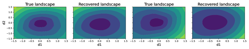
Figure 4: Ground-truth and So-Ebm recovered landscapes of the energy function in the power generator scheduling task. Darker colors represent lower energy in the heat maps. For a test sample $\mathbf{x}_{\rm test}$, we choose the corresponding optimal action $a^{*}_{\rm test}$ as the center point and select two random direction vectors $v_{1}$ and $v_{2}$ to plot the energy landscape, i.e.,$E^{{}^{\prime}}(d_{1},d_{2})=E(\mathbf{x},a^{*}+d_{1}v_{1}+d_{2}v_{2})$.

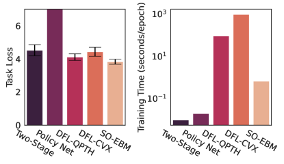
Figure 5: Results on power generator scheduling.

Results. Fig. 5 shows the end task loss for all the methods. Our method So-Ebm outperforms all the baselines with a significant reduction of training time. Compared with the strongest baseline DFL-QPTH, So-Ebm improves the task loss by $7.3\%$. The improvement is because DFL-QPTH needs to use SQP to iteratively obtain the solutions for non-quadratic optimization problems. Differentiating through all the steps of SQP is prohibitively expensive in memory and time. To address this issue, existing works donti2017task differentiate through just the last step of SQP to obtain approximate gradients. The inaccurate gradients may accrue during training and thus hurt decision quality. This shows that our explicit differentiable energy-based function is an effective surrogate for the original implicit optimization layer. In term of efficiency, So-Ebm is more than $\bm{136}$ times faster than DFL-QPTH (0.68 second/epoch v.s. 93.12 second/epoch) in training. This is because we only need to draw samples from a simple mixture of Gaussians to estimate the model parameters instead of solving and differentiating through the optimization problem at every training iteration. DFL-CVX is even slower than DFL-QPTH since it needs to use sample average estimation to draw multiple samples from $p(y|\mathbf{x};\theta)$, which results in a much more complicated optimization objective. This is also likely the reason why DFL-CVX underperforms DFL-QPTH in terms of task loss here. For Policy-Net, we have tuned its hyper-parameters extensively but still cannot achieve good performance on this task (2x-3x larger task loss than the two-stage baseline). This is not surprising: as aforementioned, Policy-Net is a pure end-to-end model that needs a large amount of data to rediscover the algorithmic structure of the optimization task. In contrast, DFL and So-Ebm model the predict-and-optimize structure in the model design, which save learning and are more data-efficient.

Fig. 4 shows the ground-truth and So-Ebm learned landscapes of the energy function. As we can see, So-Ebm can recover the landscape of the original optimization objective effectively though with a small discrepancy. The small discrepancy is expected since the ground-truth landscape is computed by directly using the ground-truth label, while So-Ebm uses the uncertainty-aware neural network to first forecast the distribution of the label and then uses the predictive distribution to compute the expected task loss as the energy function.

4.2 Resource Allocation for COVID-19

As seen in the COVID-19 pandemic, an increasing number of infected patients leads to increasing demand for medical resources; which makes it challenging for policymakers and epidemiologists to plan ahead. Mechanistic epidemiological models based on Ordinary Differential Equations (ODEs) are often used to capture and forecast the dynamics of epidemics including for the COVID-19 pandemic li2020substantial ; kain2021chopping ; hao2020reconstruction ; cui2021information . Such forecasts are typically then used as guidance to help plan for future resource allocation moghadas2020projecting ; ihme2020modeling ; rodriguez2021deepcovid ; kamarthi2021doubt . In this task, we study the optimization problem of hospital bed preparation for COVID-19, one of the most common and important tasks epidemiologists focus on during the pandemic altieri2020curating ; cramer2022evaluation . We need to decide how many beds $a\in\mathbb{R}^{7}$ are needed to prepare for the next week based on the forecasted number of hospitalized patients $y\in\mathbb{R}^{7}$. The optimization objective is a combination of linear and quadratic costs, which accounts for over-preparations $[a-y]_{+}$ and under-preparations $[y-a]_{+}$ in the next 7 days over ODE-derived dynamics:

$$\text{minimize}_{a\in\mathbb{R}^{7}}\sum_{i=1}^{7}c_{b}[y_{i}-a_{i}]_{+}+c_{h}[a_{i}-y_{i}]_{+}+q_{b}([y_{i}-a_{i}])^{2}_{+}+q_{h}([a_{i}-y_{i}])^{2}_{+}.$$ (8)

Experiment Setup. We use the SEIR+HD ODE model proposed in kain2021chopping to capture the dynamics of the COVID-19 pandemic, which has been used in policy studies for interventions. The model is driven by a key parameter: the transmission rate $\beta$ that reflects the probability of disease transmission. The forecasting model is a two-layer gated recurrent unit (GRU) chung2014empirical which takes the number of people in each state of the SEIR+HD model in the last 21 days as input features and outputs the transmission rate $\beta$ for the next 7 days. We assume that $\beta$ follows a Gaussian distribution. Since SEIR-HD is a complex non-linear ODE system, there is no closed expression for the distribution of the number of hospitalized patients $y$. Hence, we choose to sample from the forecasted distribution of $\beta$ 100 times and then simulate the SEIR-HD model to obtain the empirical distribution of the number of hospitalized patients $y$.

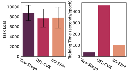
Figure 6: Results on Covid-19 resource allocation.

Results. Fig. 6 shows the results on the resource allocation for COVID-19 task. Both So-Ebm and DFL significantly outperforms the two-stage model in terms of the task loss, yielding $10.9\%+$ improvement. DFL-QPTH is not included here because it needs to use SQP to iteratively approximate the objective and is much slower than DFL-CVX in this task. The performance of So-Ebm and DFL are similar, however, the training time of So-Ebm is 4.3 times faster than DFL. The time improvement of So-Ebm is not as large as on the energy scheduling task because all the methods need to compute the complex ODE equations in the forward pass which is a time consuming part. Therefore, considering the overall training efficiency, we argue that So-Ebm is a better option than DFL on this task in practice.

4.3 Network Security Game

In this task, we study stochastic optimization in network security games wang2020automatically . Given a network $G=(V,E)$, a source node $s\in V$, and a set of target nodes $T\in V$, a network security game (NSG) washburn1995two ; fischetti2019interdiction ; roy2010survey defines the min-max game where the attacker attempts to travel from $s$ to any $t\in T$ while the defender places checkpoints on certain number of edges in the graph. Each of the target node has a reward $u(t)$ should the attacker reach them. The defender first chooses a mixed strategy. Having observed the defender’s mixed strategy but not the sampled pure strategy, the attacker attempts to choose a path. To minimize the attacker’s scores, the defender can try to predict the attacker’s path decisions with node features and their past decisions, since the attacker is not perfectly rational in reality. Suppose that $\mathbf{a}$ defines the placement of checkpoints by the defender where $\mathbf{a}_{e}$ is the probability that edge $e$ is covered. The attackers will perform a random walk on the graph, generating a path $r$, stopping at either a target or a checkpoint. The transition between two nodes is determined by the defender’s strategy $\mathbf{a}$ and node-level parameters $\mathbf{y}$, where $\mathbf{y}_{u}$ defines the “attractiveness” of node $u$, representing the attacker’s idiosyncratic preferences. The defender wants to choose $\mathbf{a}$ to maximize its expected utility: $\max_{\mathbf{a}}\mathbb{E}_{T\sim\mathbf{a}}\mathbb{E}_{r\sim p(r|\mathbf{a},\mathbf{y})}-g(r),$ where $T$ is covered edges sampled according to $\mathbf{a}$, $g(r)=u(t)$ if the attacker reaches target $t$ with path $r$ and 0 if the attacker is stopped at a checkpoint. The defender’s objective comes with the constraint $\sum\mathbf{a}\leq k$, where $k=3$ represents the resources available to the defender. The optimization objective is non-convex due to the irrational strategy of the attacker wang2020scalable .

Setup. We follow the setup of wang2020automatically , see supplementary for details.

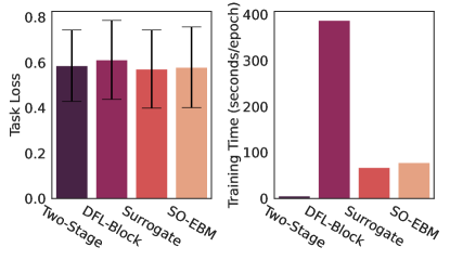
Figure 7: Results on network security game.

Results. Fig. 7 shows the results on the adversarial network security game task. Since the original DFL fails on this large scale problem, we compare a block-variable sampling approach specialized to this task (DFL-Block)wang2020scalable . Surrogate wang2020automatically performs a linear dimension reduction for DFL to speed up the training time and improve the performance by smoothing the training landscape. We did not present the results of Surrogate in the previous two tasks because the numbers of decision variables there are relatively small and it has even worse performance than the original DFL approach. As we can see, So-Ebm can achieve competitive task loss with Surrogate and outperforms DFL-block and the two-stage method. The increase of training time in our method is mainly because every evaluation of the defender’s utility requires a matrix inverse; our method needs to evaluate the utility for all the samples drawn from the proposal distribution which results a larger matrix to inverse. However, this issue can be mitigated by using some advanced matrix inverse algorithm csanky1975fast ; krishnamoorthy2013matrix . DFL-Block is even worse than the two-stage model because it back-propagates through randomly sampled variables which results in inaccruate gradient estimation.

4.4 Ablation Study

Method	Task loss
Two-stage	$4.52\pm 0.33$
So-Ebm w/o MLE	$4.31\pm 0.17$
So-Ebm w/o KLD	$3.89\pm 0.18$
So-Ebm w/ CD-LD	$3.85\pm 0.13$
So-Ebm	$\bm{3.83\pm 0.15}$

Table 1: Ablation study on power generator scheduling.

We investigate the effectiveness of the coupled training objective and alternative EBM training algorithms via ablation studies on the load forecasting and generator scheduling task. Table 1 shows the results. Our findings can be summarized as follows: (1) Both the MLE and KLD training objectives work and outperform the two-stage model. This verifies the effectiveness of using the energy-based surrogate function to approximate the optimization landscape. (2) By dropping either the MLE or KLD term, we observe a performance degradation in our method. Specifically, without the MLE term, the task loss increases by $13\%$; without KLD term, the task loss increases by $2\%$. The larger degradation when simply minimizing the KLD term is possibly because accurately recover the entire optimization landscape is too difficult and it needs the MLE term to help capture the location of the optimal decision. (3) Training So-Ebm with Contrastive Divergence based Langevin Dynamics (CD-LD) du2019implicit achieves similar performance but incurs longer training time (1.47 second/epoch v.s. 0.68 second/epoch). This phenomenon is likely because the optimization problem is relatively low-dimensional, thus importance sampling works well and enjoys better efficiency in this regime. However, even with CD-LD, So-Ebm is still 63 times faster than DFL-QPTH (1.47 second/epoch v.s. 93.12 second/epoch).

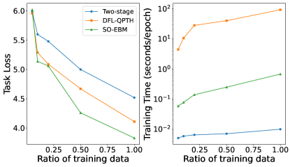
Figure 8: Task losses and training time under different ratios of training data on power generator scheduling.

We also investigate the impact of training data size for each method. Fig. 8 provides the task losses and training time under different ratios of training data on the load forecasting and generator scheduling task. As we can see, our method outperforms the baselines constantly except for the ratio of $0.05$. When the ratio is below $0.05$, all the methods cannot work properly due to the extremely low resource. The superior performance of our method is because we design the energy function as the expected task loss, which leverages the algorithmic structure inherent in the optimization problem. Hence, our method is not very data demanding. In terms of efficiency, our method reduces the training time significantly compared with DFL-QPTH across different amounts of training data.

5 Additional Related Work

The DFL works described in Section 2 focus on continuous optimization. There are also studies that extend DFL for combinatorial optimization. wilder2019melding relaxes the discrete decision into its continuous counterpart and adds a quadratic regularization term to avoid vanishing gradients. mandi2020interior proposes a log barrier regularizer and differentiates through the homogeneous self-dual embedding. mulamba2020contrastive proposes a noise contrastive objective by maximizing the distance between the optimal solution and noisy samples. Our framework may be also extended for combinatorial problems by using discrete energy-based model dai2020learning . The SPO+ loss elmachtoub2022smart has been proposed to measure the prediction errors against optimization objectives, but it is only applicable to linear programming. ProjectNet cristian2022end approximately solves the linear programming problems using a differentiable projection architecture. Our work is also related to learning to optimize vinyals2015pointer ; li2016learning ; khalil2017learning , which learns a policy network that solves optimization problems using supervised or reinforcement learning. However, these pure approaches need to rediscover the structure of the optimization problem and thus data-inefficient.

6 Limitations and Discussion

We focused on addressing the scalability and generality of existing decision-focused learning (DFL) for end-to-end stochastic optimization. We argue that these deficiencies stem from the reliance of implicitly differentiable optimization layers based on KKT conditions. As a remedy, we circumvent such deficiencies by replacing the implicit optimization layer with a newly parameterized energy-based surrogate function. We proposed a coupled training objective to encourage the energy-based surrogate well approximate the optimization landscape, as well as an efficient training procedure based on self-normalized importance sampling. Empirically, we demonstrated that our energy-based model is effective in a wide range of stochastic optimization problems with either convex or nonconvex objectives. It can achieve better or comparable performance than state-of-the-art DFL methods for stochastic optimization, while being several times or even orders of magnitude faster.

We discuss limitations and possible extensions of So-Ebm: (1) Handling more complex constraints. Our method handles the constraints implicitly through the pre-processing step and explicitly through the inference step. However, when the feasible space is extremely small, training the constrained EBM may have more benefits. To train EBMs in the constrained space, one direction is to project samples into the feasibility space. Another direction is to explore adding soft constraints to the energy function during training, e.g., Augmented Lagrangian penalty and Barrier penalty. (2) More effective training methods. Our method is a general framework for end-to-end stochastic programming problem based on EBM. There are a number of training techniques song2021train that can be plugged into our framework and we can further improve the task performance using the advanced EBM training algorithms du2021improved ; nijkamp2021mcmc .

Acknowledgments: We thank the anonymous reviewers for their helpful comments. This work was supported in part by the NSF (Expeditions CCF-1918770, CAREER IIS-2028586, IIS-2027862, IIS-1955883, IIS-2106961, IIS-2008334, CAREER IIS-2144338, PIPP CCF-2200269), CDC MInD program, faculty research award from Facebook and funds/computing resources from Georgia Tech.

Checklist

1. For all authors…

   1. Do the main claims made in the abstract and introduction accurately reflect the paper’s contributions and scope? [Yes]

   2. Did you describe the limitations of your work? [Yes]

   3. Did you discuss any potential negative societal impacts of your work? [No]

   4. Have you read the ethics review guidelines and ensured that your paper conforms to them? [Yes]

2. If you are including theoretical results…

   1. Did you state the full set of assumptions of all theoretical results? [N/A]

   2. Did you include complete proofs of all theoretical results? [N/A]

3. If you ran experiments…

   1. Did you include the code, data, and instructions needed to reproduce the main experimental results (either in the supplemental material or as a URL)? [Yes]

   2. Did you specify all the training details (e.g., data splits, hyperparameters, how they were chosen)? [Yes]

   3. Did you report error bars (e.g., with respect to the random seed after running experiments multiple times)? [Yes]

   4. Did you include the total amount of compute and the type of resources used (e.g., type of GPUs, internal cluster, or cloud provider)? [Yes]

4. If you are using existing assets (e.g., code, data, models) or curating/releasing new assets…

   1. If your work uses existing assets, did you cite the creators? [Yes]

   2. Did you mention the license of the assets? [Yes]

   3. Did you include any new assets either in the supplemental material or as a URL? [Yes]

   4. Did you discuss whether and how consent was obtained from people whose data you’re using/curating? [N/A]

   5. Did you discuss whether the data you are using/curating contains personally identifiable information or offensive content? [N/A]

5. If you used crowdsourcing or conducted research with human subjects…

   1. Did you include the full text of instructions given to participants and screenshots, if applicable? [N/A]

   2. Did you describe any potential participant risks, with links to Institutional Review Board (IRB) approvals, if applicable? [N/A]

   3. Did you include the estimated hourly wage paid to participants and the total amount spent on participant compensation? [N/A]

Supplementary Material for End-to-End Stochastic Optimization with Energy-Based Model

S. 1 Energy-based Model

The underpinning of energy-based models (EBMs) [36] is the fact that any probability density $p(\mathbf{x};\theta)$ can be expressed as:

$$p(\mathbf{x};\theta)=\frac{\text{exp}(-E(\mathbf{x};\theta))}{Z(\theta)},$$

where $E(\mathbf{x};\theta):\mathbb{R}^{D}\rightarrow\mathbb{R}$ is a nonlinear regression function that maps each input data to an energy scalar; and $Z(\theta)=\int\text{exp}(-E(\mathbf{x};\theta))d\mathbf{x}$ is a normalizing constant, also known as partition function. In this energy-based parameterization, data points with high likelihood have low energy, while data points with low likelihood have high energy. Due to its simplicity and flexibility, EBMs have been widely used in many learning tasks, including image generation [15, 59], out-of-distribution detection [20, 39], and density estimation [49, 56].

S. 2 Derivation for Eq. 6

To obtain the gradient of the model parameters, we first derive $\frac{\partial\text{log}(Z(\mathbf{x};\theta))}{\partial\theta}$:

$$\frac{\partial\text{log}Z(\mathbf{x};\theta)}{\partial\theta} =\frac{\partial\text{log}\int\text{exp}(-E(a,\mathbf{x};\theta))da}{\partial\theta}$$

$$=\left(\int\text{exp}(-E(a,\mathbf{x},a;\theta))da\right)^{-1}\frac{\partial\int\text{exp}(-E(\mathbf{x},a;\theta))da}{\partial\theta}$$

$$=\left(\int\text{exp}(-E(a,\mathbf{x},a;\theta))da\right)^{-1}\frac{\int\partial\text{exp}(-E(\mathbf{x},a;\theta))da}{\partial\theta}$$

$$=\left(\int\text{exp}(-E(a,\mathbf{x},a;\theta))da\right)^{-1}\int\text{exp}(-E(a,\mathbf{x};\theta))\left(-\frac{\partial E(a,\mathbf{x};\theta)}{\partial\theta}\right)da$$

$$=\int\left(\int\text{exp}(-E(a,\mathbf{x},a;\theta))da\right)^{-1}\text{exp}(-E(a,\mathbf{x};\theta))\left(-\frac{\partial E(a,\mathbf{x};\theta)}{\partial\theta}\right)da$$

$$=\int\frac{\text{exp}(-E(a,\mathbf{x};\theta))}{Z(\mathbf{x};\theta)}\left(-\frac{\partial E(a,\mathbf{x};\theta)}{\partial\theta}\right)da$$

$$=\int q(a|\mathbf{x};\theta)\left(-\frac{\partial E(a,\mathbf{x};\theta)}{\partial\theta}\right)da$$

$$=-\mathbb{E}_{q(a|\mathbf{x};\theta)}\frac{\partial E(a,\mathbf{x};\theta)}{\partial\theta}.$$

Then the gradient of the model parameters is given by:

$$\frac{\partial\mathcal{L}_{\text{Total}}}{\partial\theta} =\frac{\partial\mathcal{L}_{\text{MLE}}}{\partial\theta}+\lambda\frac{\partial\mathcal{L}_{\text{KL}}}{\partial\theta}$$

$$=\mathbb{E}_{(\mathbf{x},a^{*})\sim\mathcal{D}_{a}}\left(\frac{\partial E(a^{*},\mathbf{x};\theta)}{\partial\theta}+\frac{\partial\text{log}(Z(\mathbf{x};\theta))}{\partial\theta}\right)$$

$$+\lambda\mathbb{E}_{(\mathbf{x},y)\sim\mathcal{D}}\left(-\frac{\partial\mathbb{E}_{p(\hat{a}|y)}\text{log}q(\hat{a}|\mathbf{x};\theta)}{\partial\theta}-\cancelto{0}{\frac{\partial\mathcal{H}(p(a|y))}{\partial\theta}}\right)$$

$$=\mathbb{E}_{(\mathbf{x},a^{*})\sim\mathcal{D}_{a}}\left(\frac{\partial E(a^{*},\mathbf{x};\theta)}{\partial\theta}+\frac{\partial\text{log}(Z(\mathbf{x};\theta))}{\partial\theta}\right)$$

$$+\lambda\mathbb{E}_{(\mathbf{x},y)\sim\mathcal{D}}\left(\mathbb{E}_{p(\hat{a}|y)}\frac{\partial E(\hat{a},\mathbf{x};\theta)}{\partial\theta}+\frac{\partial\mathbb{E}_{p(\hat{a}|y)}\text{log}(Z(\mathbf{x};\theta))}{\partial\theta}\right)$$

$$=\mathbb{E}_{(\mathbf{x},a^{*})\sim\mathcal{D}_{a}}\left(\frac{\partial E(a^{*},\mathbf{x};\theta)}{\partial\theta}+\frac{\partial\text{log}(Z(\mathbf{x};\theta))}{\partial\theta}\right)$$

$$+\lambda\mathbb{E}_{(\mathbf{x},y)\sim\mathcal{D}}\left(\mathbb{E}_{p(\hat{a}|y)}\frac{\partial E(\hat{a},\mathbf{x};\theta)}{\partial\theta}+\frac{\partial\text{log}(Z(\mathbf{x};\theta))}{\partial\theta}\right)$$

$$=\mathbb{E}_{(\mathbf{x},a^{*})\sim\mathcal{D}_{a}}\left(\frac{\partial E(a^{*},\mathbf{x};\theta)}{\partial\theta}-\mathbb{E}_{q(\tilde{a}|\mathbf{x};\theta)}\frac{\partial E(\tilde{a},\mathbf{x};\theta)}{\partial\theta}\right)$$

$$+\lambda\mathbb{E}_{(\mathbf{x},y)\sim\mathcal{D}}\left(\mathbb{E}_{p(\hat{a}|y)}\frac{\partial E(\hat{a},\mathbf{x};\theta)}{\partial\theta}-\mathbb{E}_{q(\tilde{a}|\mathbf{x};\theta)}\frac{\partial E(\tilde{a},\mathbf{x};\theta)}{\partial\theta}\right).$$

S. 3 Training Algorithm for So-Ebm

We adopt gradient-based method such as Adam [30] to update the model parameters. At each epoch, we need to draw samples from the distributions $q(a|\mathbf{x};\theta)$ and $p(a|y)$ to estimate the gradient of the model parameters. Based on the self-normalized importance sampler, we first sample a set of $M$ candidates $\{a^{m}\}_{m=1}^{M}$ from a proposal distribution $\pi(a|\mathbf{x})$, and then sample from the empirical distribution located at each $a^{m}$ and weighted proportionally to $\text{exp}(-E(a|\mathbf{x};\theta))/\pi(a|\mathbf{x})$ and $\text{exp}(-f(y,a))/\pi(a|\mathbf{x})$. Then, we compute the gradient of the model parameters using these empirical samples according to Eq. 6. We summarize the overall training procedure in Alg. 1.

Algorithm 1 Training of So-Ebm

1:Training data $\mathcal{D}=\{(\mathbf{x}_{i},y_{i})\}_{i=1}^{N}$, task loss function $f(y,a)$, model $\mathbf{M}$ parameterized with parameter $\theta$

2:Construct feature-decision pairs $\mathcal{D}_{a}=\{(\mathbf{x}_{i},a_{i}^{*})\}$ by solving $a^{*}=\operatorname{arg\,min}_{a\in C}f(y_{i},a)$ for each $({\mathbf{x}_{i},y_{i}})$ in $\mathcal{D}$

3:$E(\mathbf{x},a;\theta)\triangleq-\mathbb{E}_{p(y|\mathbf{x};\theta)}f(y,a)$

4:for  $\#$ training iterations do

5:     Sample a mini-batch $\mathcal{B}_{y}$ from $\mathcal{D}$ and $\mathcal{B}_{a}$ from $\mathcal{D}_{a}$

6:     for For each $(\mathbf{x}_{i},a^{*}_{i})$ and $(\mathbf{x}_{i},y_{i})$ in $\mathcal{B}_{a}$ and $\mathcal{B}_{y}$  do $\triangleright$ Self-normalized importance Sampler

7:         $\pi(a;\mathbf{x}_{i})\triangleq\frac{1}{K}\sum_{k=1}^{K}\mathcal{N}(a^{*}_{i};\sigma_{k})$

8:         for $m=1,\cdots,M$ do

9:              Sample $a^{m}_{i}\sim\pi(a;\mathbf{x}_{i})$

10:              Compute $\tilde{w}(a^{m}_{i})=\text{exp}(-E(\mathbf{x}_{i},a_{i}^{m};\theta))/\pi(a^{m}_{i};\mathbf{x}_{i})$

11:              Compute $\hat{w}(a^{m}_{i})=\text{exp}(-f(y_{i},a_{i}^{m}))/\pi(a^{m}_{i};\mathbf{x}_{i})$

12:         end for

13:         Compute $\tilde{Z}=\sum_{m=1}^{M}\tilde{w}(a^{m}_{i})$, $\hat{Z}=\sum_{m=1}^{M}\hat{w}(a_{i}^{m})$

14:         $q(\tilde{a}|\mathbf{x}_{i};\theta)\triangleq\sum_{m=1}^{M}\frac{\tilde{w}(a_{i}^{m})}{\tilde{Z}}\delta_{a_{i}^{m}}(\tilde{a})$

15:         $p(\hat{a}|y)\triangleq\sum_{m=1}^{M}\frac{\hat{w}(a_{i}^{m})}{\hat{Z}}\delta_{a_{i}^{m}}(\hat{a})$

16:     end for

17:     Compute $\frac{\partial\mathcal{L}_{\text{Total}}}{\partial\theta}$ via Eq. 6 using $\mathcal{B}_{y}$, $\mathcal{B}_{a}$, $q(\tilde{a}|\mathbf{x}_{i};\theta)$ and $p(\hat{a}|y)$.

18:     Update $\theta$ using ADAM

19:end for

S. 4 Experimental Details

S. 4.1 Load Forecasting and Generator Scheduling

Closed-form expression of the expected objective. Given the electricity demand $y\in\mathbb{R}^{24}$ for the next 24 hours, the electricity scheduling problem is to decide how much electricity $a\in\mathbb{R}^{24}$ to schedule. The optimization objective is given by

$$\begin{split}&\text{minimize}_{a\in\mathbb{R}^{24}}\sum_{i=1}^{24}\mathbf{E}_{y\sim p(y|x;\theta)}[\gamma_{s}[y_{i}-a_{i}]_{+}+\gamma_{e}[a_{i}-y_{i}]_{+}+\frac{1}{2}(a_{i}-y_{i})^{2}]\\ &\quad\text{subject to}\quad|a_{i}-a_{i-1}|\leq c_{r}\quad\forall i,\end{split}$$

where $c_{r}$ is the ramp constraint and $\gamma_{s}$, $\gamma_{e}$ are the under-generation penalty and over-generation penalty respectively.

Following [13], we assume $y_{i}$ follows a Gaussian distribution with mean $\mu_{i}$ and variance $\sigma_{i}$ and obtain the closed form expression:

$$\begin{split}&\sum_{i=1}^{24}\mathbf{E}_{y\sim p(y|x;\theta)}[\gamma_{s}[y_{i}-a_{i}]_{+}+\gamma_{e}[a_{i}-y_{i}]_{+}+\frac{1}{2}(a_{i}-y_{i})^{2}]\\ &=\sum_{i=1}^{24}(\gamma_{s}+\gamma_{e})(\sigma_{i}^{2}p(a_{i};\mu_{i},\sigma_{i}^{2})+(a_{i}-\mu_{i})F(a_{i},\mu_{i},\sigma_{i}^{2}))-\gamma_{s}(a_{i}-\mu_{i})+\frac{1}{2}((a_{i}-\mu_{i})^{2}+\sigma^{2}_{i}).\end{split}$$ (9)

where $p(a;\mu,\sigma^{2})$ and $F(a;\mu,\sigma^{2})$ denote the Gaussian probability density function (PDF) and cumulative distribution function (CDF), respectively with the given mean and variance. Eq. 9 is a convex function of $a$ since the expectation of a convex function is still convex.

Model hyperparameters. We use a two-hidden-layer neural network, where each “layer” is a combination of linear, batch norm [24], ReLU, and dropout ($p=0.2$) layers with dimension $200$. So-Ebm draws $512$ samples from the proposal distribution to estimate the gradient of the model parameters. The proposal distribution is a mixture of Gaussians with 3 components where the variances are $\{0.02,0.05,0.1\}$. The weight parameter $\lambda$ that balances the MLE and KLD terms is set to $1$. DFL-CVX draws 50 samples from $p(y|\mathbf{x};\theta)$ to estimate the expectation of the task loss since it cannot use the closed-form expression.

Model optimization. We use the Adam [30] algorithm for model optimization. The number of training epochs is 100. The learning rate is selected from $\{10^{-3},10^{-4},5\times 10^{-5},10^{-5}\}$ based on the task loss on the validation set. Specifically, the learning rate for the two-stage model and PolicyNet is $10^{-3}$. The learning rate for DFL-QPTH and DFL-CVX is $10^{-4}$. The learning rate for So-Ebm is $5\times 10^{-5}$. DFL-QPTH, DFL-CVX and So-Ebm use the two-stage model as the pre-trained model for faster training convergence.

S. 4.2 Resource Allocation for COVID-19

The dataset contains the number of hospitalized patients in California from 3/29/2020 to 12/18/2021. We use the first 70% data as the training and validation sets, the remaining as the testing set. In the first 70% data, we randomly select 80% as the training set and the remaining is used as the validation set. For the optimization objective, we set $c_{b}=10$, $c_{h}=1$, $q_{b}=2$ and $q_{h}=0.5$.

Model hyperparameters. We use a two-layer gated recurrent unit (GRU) with hidden-size $128$ as the forecasting model. So-Ebm draws 512 samples from the proposal distribution to estimate the gradient of the model parameters. The proposal distribution is a mixture of Gaussians with 3 components where the variances are $\{5,10,20\}$. The weight parameter $\lambda$ that balances the MLE and KLD terms is set to $1$.

Model optimization. We use the Adam [30] algorithm for model optimization. The number of training epochs is 50. The learning rate is selected from $\{10^{-2},10^{-3},10^{-4}\}$ based on the task loss on the validation set. Specifically, the learning rate for the two-stage model and DFL-QPTH is $10^{-2}$. The learning rate for So-Ebm is $10^{-3}$. DFL-CVX and So-Ebm use the two-stage model as the pre-trained model for faster training convergence.

S. 4.3 Network Security Game

Dataset generaton. Following [54, 53], we generate random geometric graphs with 100 nodes. The generated graphs have a radius of $0.2$ in unit square. 5 nodes are chosen randomly as targets with rewards $u(t)\sim\mathcal{U}(5,10)$. 5 other nodes are sampled as candidate source nodes, from which the attacker chooses uniformly. For any node not $v$ in the node set, its attractiveness score $y_{v}$ is proportional to its distance to the closest target in with an additional uniformly distributed noise $\mathcal{U}(-1,1)$, representing the attacker’s distinct preferences. The node features $\mathbf{x}$ are computed with a Graph convolutional network (GCN) [32]: $\mathbf{x}=\mathrm{GCN}(y)+0.2\mathcal{N}(0,1)$. In this experiment, we use a randomly initialized GCN which has 4 convolutional layers and 3 fully connected layers. In this way we generate random node features correlated with their attractiveness scores and nearby node features. This is a realistic setting since neighboring locations are supposed to have similar features. The defender uses a different GCN model for prediction, which has 2 convolutional and 2 fully connected layers, ensuring that the defender’s model is less complex than the true generative mechanics. With the described procedure we sample 35 random $(\mathbf{x},y)$ pairs for the training set, 5 for the validation set, and 10 for the testing set.

Model hyperparameters. We follow [54] to configure the forecasting model. Specifically, we employ a two-layer GCN with output dimensions equal to 16 and average all node representations as the whole graph representation. The whole graph representation is further fed into a linear network with two fully-connected layers in which the hidden dimension is set to 32. So-Ebm draws 512 samples from the proposal distribution to estimate the gradient of the model parameters. The proposal distribution is a mixture of Gaussians with 3 components where the variances are $\{0.01,0.05,0.1\}$. The weight parameter $\lambda$ that balances the MLE and KLD terms is set to $1$. The reparameterization size of Surrogate is set to 10 as suggested in [54].

Model optimization. We use the Adam [30] algorithm for model optimization. All the methods are trained for at most 100 epochs and early stopped when 3 consecutive non-improving epochs occur on the validation set. Following [54], the learning rate for the two-stage model, CVX-block and Surrogate is set to $10^{-2}$. The learning rate for So-Ebm is $10^{-3}$.

S. 5 Visualization using Synthetic Dataset

To visualize whether So-Ebm can recover the landscape of the optimization objective effectively, we conduct experiments on a 2-D synthetic dataset. We generate $500$ features $\mathbf{x}\in\mathbb{R}^{2}$ from the uniform distribution $\mathcal{U}[-2,2]$. The label $y\in\mathbb{R}^{2}$ is generated by $y_{i}=x_{i}^{2}+0.03\mathcal{N}(0,1)$ for each dimension independently. The optimization objective is:

$$\text{minimize}_{a\in\mathbb{R}^{2}}\mathbb{E}_{p(y|\mathbf{x};\theta)}\sum_{i=1}^{2}3|a_{i}-y_{i}|+0.5(a_{i}-1.5)^{2}.$$ (10)

We randomly select $80\%$ data as the training set and the remaining is used for testing. The network architecture and model hyperparameters are the same as those we used in the load forecasting and generator scheduling task.

Fig. 9 shows the ground-truth and So-Ebm learned landscapes of the optimization objectives. As we can see, So-Ebm can recover the landscape of the original optimization objective effectively though with a small discrepancy. The small discrepancy is reasonable since the ground-truth landscape is computed by directly using the ground-truth label, while So-Ebm uses the uncertainty-aware neural network to first forecast the distribution of the label and then uses the predictive distribution to compute the expected task loss.

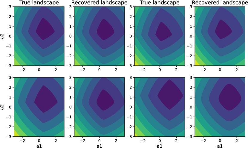
Figure 9: Ground-truth and So-Ebm recovered landscapes of the optimization objective. Darker colors represent smaller task loss in the heat maps.

S. 6 Computing Infrastructure

System: Ubuntu 18.04.6 LTS; Python 3.9; Pytorch 1.11. CPU: Intel(R) Xeon(R) Silver 4214 CPU @ 2.20GHz. GPU: GeForce GTX 2080 Ti.

References

- [1] Akshay Agrawal, Brandon Amos, Shane Barratt, Stephen Boyd, Steven Diamond, and J Zico Kolter. Differentiable convex optimization layers. Advances in neural information processing systems, 32, 2019.
- [2] Akshay Agrawal, Robin Verschueren, Steven Diamond, and Stephen Boyd. A rewriting system for convex optimization problems. Journal of Control and Decision, 5(1):42–60, 2018.
- [3] Nick Altieri, Rebecca L Barter, James Duncan, Raaz Dwivedi, Karl Kumbier, Xiao Li, Robert Netzorg, Briton Park, Chandan Singh, Yan Shuo Tan, et al. Curating a covid-19 data repository and forecasting county-level death counts in the united states. arXiv preprint arXiv:2005.07882, 2020.
- [4] Brandon Amos and J Zico Kolter. Optnet: Differentiable optimization as a layer in neural networks. In International Conference on Machine Learning, pages 136–145. PMLR, 2017.
- [5] Michael L. Bynum, Gabriel A. Hackebeil, William E. Hart, Carl D. Laird, Bethany L. Nicholson, John D. Siirola, Jean-Paul Watson, and David L. Woodruff. Pyomo–optimization modeling in python, volume 67. Springer Science & Business Media, third edition, 2021.
- [6] Junyoung Chung, Caglar Gulcehre, KyungHyun Cho, and Yoshua Bengio. Empirical evaluation of gated recurrent neural networks on sequence modeling. arXiv preprint arXiv:1412.3555, 2014.
- [7] Estee Y Cramer, Evan L Ray, Velma K Lopez, Johannes Bracher, Andrea Brennen, Alvaro J Castro Rivadeneira, Aaron Gerding, Tilmann Gneiting, Katie H House, Yuxin Huang, et al. Evaluation of individual and ensemble probabilistic forecasts of covid-19 mortality in the united states. Proceedings of the National Academy of Sciences, 119(15):e2113561119, 2022.
- [8] Rares Cristian, Pavithra Harsha, Georgia Perakis, Brian L Quanz, and Ioannis Spantidakis. End-to-end learning via constraint-enforcing approximators for linear programs with applications to supply chains. In AI for Decision Optimization Workshop of the AAAI Conference on Artificial Intelligence, 2022.
- [9] Laszlo Csanky. Fast parallel matrix inversion algorithms. In 16th Annual Symposium on Foundations of Computer Science (sfcs 1975), pages 11–12. IEEE, 1975.
- [10] Jiaming Cui, Arash Haddadan, ASM Ahsan-Ul Haque, Bijaya Adhikari, Anil Vullikanti, and B Aditya Prakash. Information theoretic model selection for accurately estimating unreported covid-19 infections. medRxiv, pages 2021–09, 2021.
- [11] Hanjun Dai, Rishabh Singh, Bo Dai, Charles Sutton, and Dale Schuurmans. Learning discrete energy-based models via auxiliary-variable local exploration. Advances in Neural Information Processing Systems, 33:10443–10455, 2020.
- [12] Steven Diamond and Stephen Boyd. CVXPY: A Python-embedded modeling language for convex optimization. Journal of Machine Learning Research, 17(83):1–5, 2016.
- [13] Priya Donti, Brandon Amos, and J Zico Kolter. Task-based end-to-end model learning in stochastic optimization. Advances in neural information processing systems, 30, 2017.
- [14] Yilun Du, Shuang Li, Joshua Tenenbaum, and Igor Mordatch. Improved contrastive divergence training of energy-based models. In International Conference on Machine Learning, pages 2837–2848. PMLR, 2021.
- [15] Yilun Du and Igor Mordatch. Implicit generation and modeling with energy based models. Advances in Neural Information Processing Systems, 32, 2019.
- [16] Adam N Elmachtoub and Paul Grigas. Smart “predict, then optimize”. Management Science, 68(1):9–26, 2022.
- [17] Matteo Fischetti, Ivana Ljubić, Michele Monaci, and Markus Sinnl. Interdiction games and monotonicity, with application to knapsack problems. INFORMS Journal on Computing, 31(2):390–410, 2019.
- [18] IHME COVID-19 forecasting team. Modeling covid-19 scenarios for the united states. Nature medicine, 2020.
- [19] Yarin Gal and Zoubin Ghahramani. Dropout as a bayesian approximation: Representing model uncertainty in deep learning. In international conference on machine learning, pages 1050–1059. PMLR, 2016.
- [20] Will Grathwohl, Kuan-Chieh Wang, Joern-Henrik Jacobsen, David Duvenaud, Mohammad Norouzi, and Kevin Swersky. Your classifier is secretly an energy based model and you should treat it like one. In International Conference on Learning Representations, 2020.
- [21] Xingjie Hao, Shanshan Cheng, Degang Wu, Tangchun Wu, Xihong Lin, and Chaolong Wang. Reconstruction of the full transmission dynamics of covid-19 in wuhan. Nature, 584(7821):420–424, 2020.
- [22] William E Hart, Jean-Paul Watson, and David L Woodruff. Pyomo: modeling and solving mathematical programs in python. Mathematical Programming Computation, 3(3):219–260, 2011.
- [23] Geoffrey E Hinton. Training products of experts by minimizing contrastive divergence. Neural computation, 14(8):1771–1800, 2002.
- [24] Sergey Ioffe and Christian Szegedy. Batch normalization: Accelerating deep network training by reducing internal covariate shift. In International conference on machine learning, pages 448–456. PMLR, 2015.
- [25] Eric Jang, Shixiang Gu, and Ben Poole. Categorical reparameterization with gumbel-softmax. arXiv preprint arXiv:1611.01144, 2016.
- [26] Morgan P Kain, Marissa L Childs, Alexander D Becker, and Erin A Mordecai. Chopping the tail: How preventing superspreading can help to maintain covid-19 control. Epidemics, 34:100430, 2021.
- [27] Harshavardhan Kamarthi, Lingkai Kong, Alexander Rodríguez, Chao Zhang, and B Aditya Prakash. When in doubt: Neural non-parametric uncertainty quantification for epidemic forecasting. Advances in Neural Information Processing Systems, 34, 2021.
- [28] Elias Khalil, Hanjun Dai, Yuyu Zhang, Bistra Dilkina, and Le Song. Learning combinatorial optimization algorithms over graphs. Advances in neural information processing systems, 30, 2017.
- [29] Sujin Kim, Raghu Pasupathy, and Shane G Henderson. A guide to sample average approximation. Handbook of simulation optimization, pages 207–243, 2015.
- [30] Diederik P Kingma and Jimmy Ba. Adam: A method for stochastic optimization. In International Conference on Representation Learning, 2015.
- [31] Diederik P Kingma and Max Welling. Auto-encoding variational bayes. arXiv preprint arXiv:1312.6114, 2013.
- [32] Thomas N Kipf and Max Welling. Semi-supervised classification with graph convolutional networks. arXiv preprint arXiv:1609.02907, 2016.
- [33] Anton J Kleywegt, Alexander Shapiro, and Tito Homem-de Mello. The sample average approximation method for stochastic discrete optimization. SIAM Journal on Optimization, 12(2):479–502, 2002.
- [34] Lingkai Kong, Jimeng Sun, and Chao Zhang. Sde-net: Equipping deep neural networks with uncertainty estimates. In International Conference on Machine Learning, pages 5405–5415. PMLR, 2020.
- [35] Aravindh Krishnamoorthy and Deepak Menon. Matrix inversion using cholesky decomposition. In 2013 signal processing: Algorithms, architectures, arrangements, and applications (SPA), pages 70–72. IEEE, 2013.
- [36] Yann LeCun, Sumit Chopra, Raia Hadsell, M Ranzato, and F Huang. A tutorial on energy-based learning. Predicting structured data, 1(0), 2006.
- [37] Ke Li and Jitendra Malik. Learning to optimize. arXiv preprint arXiv:1606.01885, 2016.
- [38] Ruiyun Li, Sen Pei, Bin Chen, Yimeng Song, Tao Zhang, Wan Yang, and Jeffrey Shaman. Substantial undocumented infection facilitates the rapid dissemination of novel coronavirus (sars-cov-2). Science, 368(6490):489–493, 2020.
- [39] Weitang Liu, Xiaoyun Wang, John Owens, and Yixuan Li. Energy-based out-of-distribution detection. Advances in Neural Information Processing Systems, 33:21464–21475, 2020.
- [40] C Maddison, A Mnih, and Y Teh. The concrete distribution: A continuous relaxation of discrete random variables. In Proceedings of the international conference on learning Representations. International Conference on Learning Representations, 2017.
- [41] Jayanta Mandi and Tias Guns. Interior point solving for lp-based prediction+ optimisation. Advances in Neural Information Processing Systems, 33:7272–7282, 2020.
- [42] Seyed M Moghadas, Affan Shoukat, Meagan C Fitzpatrick, Chad R Wells, Pratha Sah, Abhishek Pandey, Jeffrey D Sachs, Zheng Wang, Lauren A Meyers, Burton H Singer, et al. Projecting hospital utilization during the covid-19 outbreaks in the united states. Proceedings of the National Academy of Sciences, 117(16):9122–9126, 2020.
- [43] Maxime Mulamba, Jayanta Mandi, Michelangelo Diligenti, Michele Lombardi, Victor Bucarey, and Tias Guns. Contrastive losses and solution caching for predict-and-optimize. arXiv preprint arXiv:2011.05354, 2020.
- [44] Erik Nijkamp, Ruiqi Gao, Pavel Sountsov, Srinivas Vasudevan, Bo Pang, Song-Chun Zhu, and Ying Nian Wu. Mcmc should mix: Learning energy-based model with neural transport latent space mcmc. In International Conference on Learning Representations, 2021.
- [45] Andrew Perrault, Bryan Wilder, Eric Ewing, Aditya Mate, Bistra Dilkina, and Milind Tambe. End-to-end game-focused learning of adversary behavior in security games. In Proceedings of the AAAI Conference on Artificial Intelligence, volume 34, pages 1378–1386, 2020.
- [46] Danilo Jimenez Rezende, Shakir Mohamed, and Daan Wierstra. Stochastic backpropagation and approximate inference in deep generative models. In International conference on machine learning, pages 1278–1286. PMLR, 2014.
- [47] Alexander Rodríguez, Anika Tabassum, Jiaming Cui, Jiajia Xie, Javen Ho, Pulak Agarwal, Bijaya Adhikari, and B. Aditya Prakash. Deepcovid: An operational deep learning-driven framework for explainable real-time covid-19 forecasting. Proceedings of the AAAI Conference on Artificial Intelligence, 35(17):15393–15400, May 2021.
- [48] Sankardas Roy, Charles Ellis, Sajjan Shiva, Dipankar Dasgupta, Vivek Shandilya, and Qishi Wu. A survey of game theory as applied to network security. In 2010 43rd Hawaii International Conference on System Sciences, pages 1–10. IEEE, 2010.
- [49] Yang Song, Sahaj Garg, Jiaxin Shi, and Stefano Ermon. Sliced score matching: A scalable approach to density and score estimation. In Uncertainty in Artificial Intelligence, pages 574–584. PMLR, 2020.
- [50] Yang Song and Diederik P Kingma. How to train your energy-based models. arXiv preprint arXiv:2101.03288, 2021.
- [51] Bram Verweij, Shabbir Ahmed, Anton J Kleywegt, George Nemhauser, and Alexander Shapiro. The sample average approximation method applied to stochastic routing problems: a computational study. Computational optimization and applications, 24(2):289–333, 2003.
- [52] Oriol Vinyals, Meire Fortunato, and Navdeep Jaitly. Pointer networks. Advances in neural information processing systems, 28, 2015.
- [53] Kai Wang, Andrew Perrault, Aditya Mate, and Milind Tambe. Scalable game-focused learning of adversary models: Data-to-decisions in network security games. In AAMAS, pages 1449–1457, 2020.
- [54] Kai Wang, Bryan Wilder, Andrew Perrault, and Milind Tambe. Automatically learning compact quality-aware surrogates for optimization problems. Advances in Neural Information Processing Systems, 33:9586–9596, 2020.
- [55] Alan Washburn and Kevin Wood. Two-person zero-sum games for network interdiction. Operations research, 43(2):243–251, 1995.
- [56] Li Wenliang, Danica J Sutherland, Heiko Strathmann, and Arthur Gretton. Learning deep kernels for exponential family densities. In International Conference on Machine Learning, pages 6737–6746. PMLR, 2019.
- [57] Bryan Wilder, Bistra Dilkina, and Milind Tambe. Melding the data-decisions pipeline: Decision-focused learning for combinatorial optimization. In Proceedings of the AAAI Conference on Artificial Intelligence, volume 33, pages 1658–1665, 2019.
- [58] Markus Wulfmeier, Peter Ondruska, and Ingmar Posner. Maximum entropy deep inverse reinforcement learning. arXiv preprint arXiv:1507.04888, 2015.
- [59] Junbo Zhao, Michael Mathieu, and Yann LeCun. Energy-based generative adversarial network. arXiv preprint arXiv:1609.03126, 2016.
- [60] Brian D Ziebart, Andrew L Maas, J Andrew Bagnell, Anind K Dey, et al. Maximum entropy inverse reinforcement learning. In Proceedings of the AAAI Conference on Artificial Intelligence, volume 8, pages 1433–1438. Chicago, IL, USA, 2008.