Spectral estimation for mixed causal-noncausal autoregressive models

Abstract

This paper investigates new ways of estimating and identifying causal, noncausal, and mixed causal-noncausal autoregressive models driven by a non-Gaussian error sequence. We do not assume any parametric distribution function for the innovations. Instead, we use the information of higher-order cumulants, combining the spectrum and the bispectrum in a minimum distance estimation. We show how to circumvent the nonlinearity of the parameters and the multimodality in the noncausal and mixed models by selecting the appropriate initial values in the estimation. In addition, we propose a method of identification using a simple comparison criterion based on the global minimum of the estimation function. By means of a Monte Carlo study, we find unbiased estimated parameters and a correct identification as the data depart from normality. We propose an empirical application on eight monthly commodity prices, finding noncausal and mixed causal-noncausal dynamics.

Keywords: Autorregresive; Noncausal; Mixed; Spectrum; Bispectrum; Multimodality.

1 Introduction

The traditional assumption of causality in autoregressive models is widely adopted in classical estimation methods for economic time series. The causality implies that the time series depends on a combination of lags with roots outside the unit circle, forcing the time series to depend only on past information. Despite this, causality is not always justified and is not systematically tested. Additionally, it emerges that including only past information for estimating economic models fails to explain their structural shocks, as shown by Hansen and Sargent (1991). In addition, Lanne et al. (2012); Lanne and Luoto (2012) show that including future information may improve the forecast accuracy, i.e., through noncausal model representations. A statistically rigorous presentation of noncausal models arises in Breid et al. (1991), dividing the autoregressive polynomial into two components, one causal with roots outside the unit circle and another noncausal with roots inside the unit circle, or equivalently, including leads in the autoregressive process. Furthermore, allowing the autoregressive polynomial to contain roots simultaneously inside and outside the unit circle, introduces the mixed causal-noncausal models. The noncausal dynamics offer the possibility to capture nonlinearities in weakly stationary variables, such as locally explosive patterns and bubbles, replicating characteristics of anticipation and speculation. Consequently, noncausal models can produce valuable risk measures, fueling their interest in economics, with applications in inflation, commodity prices, and stock indices, see among others Gouriéroux and Zakoïan (2017); Lof (2013); Lof and Nyberg (2017); Lanne and Saikkonen (2011); Hecq et al. (2016); Hecq and Voisin (2021).

An interesting aspect of the noncausal models is the estimation and identification. The reason is that they share the same second-order dependence structure, the autocovariance function or its frequency domain analog, the spectral density, with the causal models. Consequently, the estimations based only on second-order moments such as Gaussian-likelihood, OLS, Yule-Walker, or Whittle yield coefficients corresponding to roots outside the unit circle identifying a causal model, even though the actual roots of the coefficients are inside the unit circle, corresponding to a noncausal model. The underlying reason for this lack of identification is the assumption of Gaussianity. For the Gaussian series, the probability structure is entirely determined by second-order moments. In general, for an AR($p$) model with a Gaussian errors sequence, there exist $2^{p}$ possible specifications of its roots with the same probability structure. In contrast, when the error sequence is non-Gaussian, each of the $2^{p}$ configurations of roots corresponds to a different weakly stationary process with a unique and identifiable probability structure. Evidently, knowing the non-Gaussian probability distribution of the error sequence, the natural estimator is the Maximum Likelihood (ML), identifying the true roots of the autoregressive polynomial regardless of whether it is causal or noncausal, see Basawa et al. (1976). This estimation was initially proposed by K.-S. Lii and Rosenblatt (1992) for possible noninvertible MA models, proving that it is consistent for any symmetric, strictly positive, and sufficiently smooth non-Gaussian probability density function. Huang and Pawitan (2000) propose a quasi-Likelihood estimation of possible noninvertible MA models using the Laplacian distribution. Breid et al. (1991) proposes an Maximum likelihood estimation (MLE) for possibly noncausal autoregressive processes driven by non-Gaussian i.i.d. noise, evidencing that the estimated parameters are asymptotically normal and providing identification when the error sequence is heavy-tailed. K.-S. Lii and Rosenblatt (1996); Lehr and Lii (1998), implement MLE for possible noncausal and noninertible ARMA models. Similarly, Lanne and Saikkonen (2011), Hecq et al. (2016), Giancaterini and Hecq (2022) propose a parameter estimation in possible noncausal AR models using the Student’s t distribution. For the same distribution, Andrews et al. (2006) proposes the estimation of the all-pass ARMA models, where all roots of the autoregressive polynomial are reciprocals of roots of the moving average polynomial and vice versa. MLE for autoregressive models using the alpha-stable distribution has also been implemented in Andrews et al. (2009); Fries (2021).

A natural criticism of MLE is the prior knowledge about the probability distribution of the error sequence, which is uncommon empirically. Indeed, arbitrarily assuming a distribution function that does not replicate the features of the data can lead to misestimating parameters and misidentifying the autoregressive model. Alternatively, in this research, we propose to estimate the parameters of the causal, noncausal, and mixed autoregressive model without prior knowledge about the probability distribution of the error sequence. Instead, it has been proposed to employ the higher-order cumulants necessary for constructing the higher-order spectral densities, with the ability to discriminate between causal and noncausal models. Higher-order cumulants, also named higher-order correlations, have been used to estimate noncausal AR models, see Rosenblatt (1980); K. Lii and Rosenblatt (1982); Giannakis and Swami (1990); Tugnait (1986); Terdik (1999); Nikias and Chiang (1987). We use in this paper the procedure proposed by Brillinger (1985); Leonenko et al. (1998); Velasco and Lobato (2018), constructing a function of the second and third-order spectral densities (the spectrum and the bispectrum, respectively) in a minimum distance estimation with the periodogram and biperiodogram. The estimation of the parameters is performed by minimizing the function, achieving the identification of the model in its global minimum.

Although this estimation is consistent and asymptotically normal, the global minimum is not guaranteed to be obtained. On the contrary, the estimation function is multimodal (not convex), leading to multiple local minima that increase as the number of parameters in the model grows. Accordingly, the solution is not unique and convergent. For a discussion of the multimodality in noncausal models, see Kindop (2021), and for mixed causal-noncausal, see Bec et al. (2020). Consequently, an empirical prerequisite for reaching the global minimum in the estimation function is the appropriate selection of the initial values. In this sense, our first contribution to the literature is to develop a general scheme for selecting the initial values for estimating noncausal and mixed causal-noncausal based on their causal representations. This allows us to find the correct combination of parameters in the region where the global minimum of the estimation function lies. In our second contribution, we present a decision method for identifying the model based on the existence of the global minimum in the estimation function. We explore the robustness of our method in finite samples through an extensive Monte Carlo study using the alpha-stable distribution. We find unbiased estimated parameters and a correct identification as the data depart from normality. Our third contribution is to perform the third-order spectral estimation of mixed models. To the best of our knowledge, this is the first time in mixed models. In addition, we propose an empirical application of eight monthly commodity prices, evidencing noncausal and mixed causal/noncausal dynamics.

The paper is divided as follows: Section 2 presents the methodology, Section 3 presents the estimation method, Section 4 introduces the Monte Carlo study, Section 5 presents the empirical application, and the last Section wraps up the conclusions and discussion.

2 Methodology

Let $y_{t}$ be a time series of length $T$, with zero mean and finite $k$-th order moments, for $k\geq 2$, and $k$-th weakly stationary for $t=\left\{0,\pm 1,\pm 2,\pm 3,...\right\}$, with autocovariance function

$$\kappa_{2}(j)=\mathbb{E}\left[y_{t}y_{t-j}\right]\;\;for\;\;\ j=\left\{0,\pm 1,\pm 2,\pm 3,...\right\}.$$ (1)

Notice that the autocovariance is considering linear relations of the data in two time periods, known as second-order dependence, also that $\kappa_{2_{j}}=\kappa_{2_{j-1}}...=\kappa_{2_{j-n}}=\kappa_{2_{j+1}}...=\kappa_{2_{j+n}}$. In any of these representations, the autocovariance function remains unchanged. Therefore, estimations based on the second-order structure, e.g., Gaussian-Likelihood, OLS, or Yule-Walker, fail to distinguish between causal and noncausal models. The above is evident in Figure 1. On the left is a causal model and on the right is a noncausal model with the same coefficients and the same alpha-stable error sequence. Notice that the autocorrelation functions are identical.

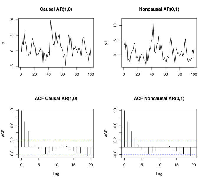
Figure 1: In the left is the causal AR(1,0) model $y_{t}=0.7y_{t-1}+\varepsilon_{t}$, and in the right, the noncausal AR(0,1) model $y_{t}=0.7y_{t+1}+\epsilon_{t}$, plot and ACF. $\varepsilon_{t}\sim$ alpha-stable $f_{a}(t;\alpha=1.5,\beta=0.25,\gamma=1,\delta=0)$. The definition of the alpha-stable distribution is in Section 4, the sample size $T=100$. The advantage of using the alpha-stable distribution is the ability to have different shapes depending on the value of its parameters. It can easily replicate sample characteristics of leptokurticity and skewness. Although theoretically, the existence of its moments is linked to the values of its stability parameter ($\alpha$), i.e., the variance, the skewness, and the kurtosis only exist when it is equal to two. An interesting feature of the alpha-stable distribution is its infinite divisibility, i.e., it can be expressed as a sum of i.i.d variables while preserving its distribution. See Section 4 for details.

However, when the time series is non-Gaussian, the probability structure of causal and noncausal models is different and identifiable using additional information from the higher-order cumulants. We specify that the first three moments are equivalent to the first three cumulants. This is not valid for cumulants of orders greater than three. In particular, the third cumulant contains the relation of the time series at three points in time. Hence it is known as the triple correlation function or the bicovariance function, see Bartelt et al. (1984). The third-order cumulant is

$$\kappa_{3}(j,l)=\mathbb{E}\left[y_{t}y_{t-j}y_{t-l}\right]\;\;for\;\;\ j,l=\left\{0,\pm 1,\pm 2,\pm 3,...\right\}.$$ (2)

Note that $\kappa_{3}(j,l)$ is equal to zero for the Gaussian and symmetrical distributions. The definition of $\kappa_{3}(j,l)$ is the third coefficient of the power expansion of the natural logarithm of the characteristic function of a random variable. Given the stationarity of $y_{t}$, $\kappa_{3}(j,l)$ satisfies the following symmetry conditions

$$\kappa_{3}(j,l)=\kappa_{3}(l,j)=\kappa_{3}(-j,l-j)=\kappa_{3}(l-j,-j)=\kappa_{3}(j-l,-l)=\kappa_{3}(-l,j-l).$$ (3)

The second and third-order cumulants are necessary for constructing the spectrum and the bispectrum. The spectrum is the Fourier transform of the second cumulant. Analogously, the bispectrum is the Fourier transform of the third-order cumulant. Defining the Fourier frequencies as $\omega=2\pi/T$, the spectrum is

$$S_{2}(\omega_{j})=\frac{1}{2\pi}\sum_{j=-\infty}^{\infty}\kappa_{2}(j)e^{-ij\omega},$$ (4)

where $i$ is the imaginary number. The bispectrum is

$$S_{3}(\omega_{1},\omega_{2})=\frac{1}{(2\pi)^{2}}\sum_{j=-\infty}^{\infty}\sum_{l=-\infty}^{\infty}\kappa_{3}(j,l)e^{-i(j\omega_{1}+l\omega_{2})}.$$ (5)

Note that for the existence of the bispectrum, the third-order cumulant must be different from zero. We assume that the spectrum and the bispectrum have continuous second-derivatives and are bounded above and away from zero in modulus for the sets of frequencies $\Lambda_{1}$ and $\Lambda_{2}$. Where $\omega_{1}\subset\Lambda_{1}=(0,1/2)$ for $S_{2}$, and given the symmetries $S_{3}(\omega_{1},\omega_{2})=S_{3}(\omega_{2},\omega_{1})=S_{3}(\omega_{1},-\omega_{2}-\omega_{1})=S_{3}(-\omega_{1}-\omega_{2},\omega_{2})$ and the identity $S_{3}(\omega_{1},\omega_{2})=S_{3}(-\omega_{1},-\omega_{2})$, $\Lambda_{2}$ is a finite union of compact sets inside an open triangle with vertices $(0,0),(1/2,0),(1/3,1/3)$, for details see Rao and Gabr (1989); Rosenblatt and Van Ness (1965); Rao and Gabr (2012); Anh et al. (2007).

The nonparametric estimation of the spectrum and bispectrum for autoregressive processes is usually based on methods employing the discrete Fourier transform (DFT), i.e., assuming that the time series comprises a set of harmonically related sinusoids. Let us define the DFT as

$$d_{T}(\omega)=\sum_{t=0}^{T-1}y_{t}e^{-it\omega}.$$ (6)

The most popular estimator of the spectrum is the periodogram. For a summary of spectrum estimates, see Kay and Marple (1981). The periodogram is obtained as the modulus of the output values from the DFT in Equation 6, performed directly on the time series. The origin of the periodogram can be traced back to Schuster (1898), which conducted a Fourier series fitting to the variation of sunspot numbers trying to find hidden periodicities in the data. Thereafter, it has been widely used in spectral analysis and autoregressive modeling, see Brillinger (1975); Rosenblatt (1965); Alekseev (1996); Bartlett (1950); Brillinger and Rosenblatt (1967). The periodogram is defined as

$$I_{2}(\omega)=\frac{1}{2\pi T}d_{T}(\omega)\overline{d_{T}(\omega)}.$$ (7)

Similar to the periodogram, however, taking into account relations between three frequencies (bifrequencies), the biperiodogram is the bispectrum estimator, defined as

$$I_{3}=(\omega_{1},\omega_{2})=\frac{1}{(2\pi)^{2}T}d_{T}(\omega_{1})d_{T}(\omega_{2})\overline{d_{T}(-\omega_{1}-\omega_{2})},$$ (8)

where $\overline{d_{T}(-\omega_{1}-\omega_{2})}$, represents the complex conjugate of the Fourier transform of the sum of two frequencies. This component is the one that accounts for the asymmetries present in non-Gaussian data. Contrary to the periodogram, which is always real, the biperiodogram is complex due to its last factor. The periodogram and biperiodogram are asymptotically unbiased estimators of the spectrum and bispectrum but inconsistent; i.e., the variance of the estimates will not tend to zero as $T$ increases without bound, see Brillinger (1975); Rosenblatt (1965); Alekseev (1996); Bartlett (1950). Some properties of the periodogram are developed in Brillinger and Rosenblatt (1967); in particular, the mean of the periodogram $k=2$ and biperiodogram $k=3$. Denoting $\bm{\omega}={\omega_{1},\omega_{2}}$

$$E[I_{k}(\bm{\omega})]=S_{k}(\bm{\omega})+o(1),$$ (9)

when $\omega_{s}\neq 0\;mod\;2\pi$. The variance for $k={2,3}$

$$T^{2-k}Var[I_{k}(\bm{\omega})]=(k-1)!S_{2}(\omega_{1})...S_{2}(\omega_{k-1})S_{2}(\omega_{1}+...+\omega_{k-1})+o(1),$$ (10)

as $T\rightarrow\infty$. Equivalently to the periodogram, the biperiodogram at different Fourier frequencies $(\omega\neq\omega^{\prime})$ is uncorrelated

$$Cov[I_{k}(\omega),I_{\iota}(\omega^{\prime})]=o(T^{\frac{k+\iota-4}{2}}),\;\;\;k,\iota=2,3.$$ (11)

2.1 The causal AR($r,0$)

In this Section, we present causal, noncausal, and mixed autoregressive models. Let $y_{t}$ be a causal autoregressive process generated by

$$\phi(L)y_{t}=\varepsilon_{t}.$$ (12)

The lag polynomial is $\phi(L)=1-\phi_{1}L-\phi_{2}L^{2}...\phi_{r}L^{r}$, with a set of parameters $\Phi_{r}=(\phi_{1},\phi_{2}...\phi_{r})$, where $L$ stands for the backward shift operator, that is, $L^{k}=y_{t-k}$ for $k=\left\{0,\pm 1,\pm 2,\pm 3,...\right\}$. This model is well known in the time series literature as the AR($p$). In our notation, the AR($p$) model is replaced by the AR($r,0$) model. The main difference between the AR($p$) model and the AR($r,0$) model is that in the former, it is sufficient to assume white noise in the error sequence, while in the latter, we assume that the error sequence is i.i.d and has finite moments greater than 3, that is

$$\mathbb{E}(\varepsilon_{t})=0,\;\;\mathbb{E}(\varepsilon_{t}^{2})=k_{2_{e}},\;\;\textrm{and}\;\;\mathbb{E}(\varepsilon_{t}^{3})=k_{3_{e}}.$$ (13)

The same assumption applies to the AR($0,s$) and MAR($r,s$) models, discussed in Sections 2.2 and 2.3, respectively. Note that we differentiate the cumulants of $y_{t}$, $\kappa_{2},\kappa_{3}$, with the cumulants of the error sequence $\varepsilon_{t}$, $\kappa_{2_{e}},\kappa_{3_{e}}$. $\phi(z)$ is provided by the roots $1-\phi_{1}z-\phi_{2}z^{2}...-\phi_{r}z^{r}$, all lying outside the unit circle. Hence, the model has a covariance-stationary representation form $\kappa_{2}(j)=\mathbb{E}\left[y_{t}y_{t-j}\right]$, and is represented as an infinite sum of past shocks, MA($\infty$) as

$$y_{t}=\Psi(L)\varepsilon_{t},$$ (14)

where $\sum_{j=0}^{\infty}\lvert\Psi\rvert<\infty$. Then, the autocovariance generating function of $y_{t}$ is $g_{y}(z)=\sum_{j=-\infty}^{\infty}\kappa_{2}(j)z^{j}$. Evaluating $g_{y}$ at $z=e^{-i\omega}$, and dividing by $2\pi$ we obtain the spectrum of $y_{t}$

$$S_{2}(\Phi_{r},\omega)=\frac{1}{2\pi}g_{y}(e^{-i\omega})=\sum_{j=-\infty}^{\infty}\kappa_{2}(j)e^{-i\omega j}.$$ (15)

This function is known as the second-order spectrum since it only considers second-order relations. The spectrum is continuous, non-negative, real-valued, symmetric, and periodic around $\omega$. For the AR($r,0$) model, the spectrum can be obtained explicitly using the representation of Equation 14. Thus, we can define the transfer function of the linear filter AR($r,0$) as

$$\psi(\Phi_{r},\omega)=1/(1-\phi_{1}z-\phi_{2}z^{2}...-\phi_{r}z^{r}).$$ (16)

Then, the spectrum of the AR($r,0$) is the multiplication of the second-order cumulant of the errors sequence and the transfer function, and its conjugate

$$\begin{split}S_{2}(\Phi_{r},\omega)&=\frac{k_{2_{e}}}{2\pi}\psi(\Phi_{r},\omega)\overline{\psi(\Phi_{r},\omega)}\\ &=\frac{k_{2_{e}}}{2\pi}\frac{1}{(1-\phi_{1}z-\phi_{2}z^{2}...-\phi_{r}z^{r})(1-\phi_{1}z^{-1}-\phi_{2}z^{-2}...-\phi_{r}z^{-r})}\\ &=\frac{k_{2_{e}}}{2\pi}\frac{1}{\lvert 1-\phi_{1}z-\phi_{2}z^{2}-...-\phi_{r}z^{r}\rvert^{2}}.\end{split}$$ (17)

Defining $\overline{z}=e^{2\pi i(-\omega_{1}-\omega_{2})}$, the transfer function of the sum of the complex conjugation of the frequencies is $\overline{\psi(\Phi_{r},-\omega_{1}-\omega_{2})}=1/(1-\phi_{1}\overline{z}-...-\phi_{2}\overline{z}^{2}-...-\overline{z}^{r})$. In this way, the bispectrum is

$$\begin{split}S_{3}(\Phi_{r},\omega_{1},\omega_{2})&=\frac{k_{3_{e}}}{(2\pi)^{2}}\psi(\Phi_{r},\omega_{1})\psi(\Phi_{r},\omega_{2})\overline{\psi(\Phi_{r},-\omega_{1}-\omega_{2})}\\ &=\frac{k_{3_{e}}}{(2\pi)^{2}}\frac{1}{(1-\phi_{1}z-\phi_{2}z^{2}...-\phi_{r}z^{r})(1-\phi_{1}z^{-1}-\phi_{2}z^{-2}...-\phi_{r}z^{-r})(1-\phi_{1}\overline{z}-\phi_{2}\overline{z}^{2}-...-\phi_{r}\overline{z}^{r})}.\\ \end{split}$$ (18)

2.2 The noncausal AR($0,s$)

Let $y_{t}$ be a noncausal autoregressive process generated by

$$\varphi(L^{-1})y_{t}=\varepsilon_{t},$$ (19)

where the lead polynomial is $\varphi(L^{-1})=1-\varphi_{1}L^{-1}-\varphi_{2}L^{-2}...\varphi_{s}L^{-s}$ with the set of parameters $\Phi_{s}=(\varphi_{1},\varphi_{2}...\varphi_{s})$. In this notation, the AR($0,s$) model has $s$ noncausal and zero causal components. The polynomial $\varphi(z)$ is $1-\varphi_{1}z-\varphi_{2}z^{2}...-\varphi_{s}z^{s}$, with all roots outside the unit circle. Note that the polynomial of the noncausal model can be represented with its roots outside the unit circle, thus depending on its leads, or with roots inside the unit circle depending on its lags. Indeed, the polynomial $\varphi(z)$ has a causal representation with its zeros inside the unit circle, (see Brockwell and Davis (1987) p. 81 for a stationary solution), that is $\varphi^{*}(z)=1-\varphi_{1}^{*}z-\varphi_{2}^{*}z^{2}...\varphi_{s}^{*}z^{s}$, with $\varphi^{*}(z)\neq 0$ for $\lvert z\rvert>1$. Following Equation 6 in Lanne and Saikkonen (2011), the polynomial $\varphi^{*}(z)$ can be expressed as

$$\varphi^{*}(z)=-\varphi^{*}_{s}z^{s}\left(1+\frac{\varphi^{*}_{s-1}}{\varphi^{*}_{s}}z^{-1}+...+\frac{\varphi^{*}_{1}}{\varphi^{*}_{s}}z^{1-s}-\frac{1}{\varphi^{*}_{s}}\right)=-\varphi^{*}_{s}z^{s}\varphi(z^{-1}),$$ (20)

where $\varphi(z^{-1})$ is as in Equation 19, implying that $\varphi^{*}_{s-j}/\varphi^{*}_{s}=-\varphi_{j}$ for $j=1,2,...s-1$, and $1/\varphi^{*}_{s}=\varphi_{j}$. Notice that the zeros of $\varphi^{*}(z)$ lie inside the unit circle. In this way, the noncausal model can be rewritten to obtain the following causal specification

$$\varphi^{*}(L)y_{t}=\xi_{t},$$ (21)

where the error term $\xi_{t}=-1/\varphi_{s}\varepsilon_{t-s}$, and coefficients for the polynomial $\varphi^{*}_{j}$ equal to $\varphi^{*}_{j}=-\varphi_{j}/\varphi_{s}$ for $j=1,2...s-1$, and $\varphi^{*}_{s}=1/\varphi_{s}$. Note that this causal representation with roots inside the unit circle should not be confused with the explosive model, where the error term is contemporaneously uncorrelated with lags of $y_{t}$ (see Brockwell and Davis (1987), p. 81). As an example, in the Remark 1, we rewrite the noncausal AR(0,$s$) into a purely causal AR($r,0$), for $s=r$.

Remark 1. The causal AR($r,0$) representation of the noncausal AR($0,s$) model, for $s=r$. The noncausal AR($0,s$) is

$$y_{t}=\varphi_{1}y_{t+1}+\varphi_{2}y_{t+2}+...+\varphi_{s}y_{t+s}+\varepsilon_{t}.$$

Reverting the process in $s$ time periods

$$y_{t-s}=\varphi_{1}y_{t+1-s}+\varphi_{2}y_{t+2-s}...\varphi_{s}y_{t}+\varepsilon_{t-s}.$$

Solving for $y_{t}$, we can rewrite $y_{t}$ as

$$y_{t}=-\frac{\varphi_{1}}{\varphi_{s}}y_{t+1-s}-\frac{\varphi_{2}}{\varphi_{s}}y_{t+2-s}+...+\frac{1}{\varphi_{s}}y_{t-s}-\frac{1}{\varphi_{s}}\varepsilon_{t-s},$$ (22)

which highlight the correlation between the error term and the regressors. Then, the purely causal AR($r,0$) representation of the AR($0,s$) is

$$y_{t}=\varphi^{*}_{1}y_{t+1-s}+\varphi^{*}_{2}y_{t+2-s}+...+\varphi^{*}_{s}y_{t-s}+\xi_{t}.$$ (23)

Notice that the coefficients and the error sequence from Equation 23 are equivalent to the ones in Equation 21. The causal representation is key to the estimation and identification of the model, as we shall discuss in Section 3.2.

The transfer function for the noncausal AR(0,$s$) is $\psi(\Phi_{s},\omega)=1/(1-\varphi_{1}z-\varphi_{2}z^{2}...-\varphi_{r}z^{s})$, and its spectrum is

$$\begin{split}S_{2}(\Phi_{s},\omega)&=\frac{k_{2_{e}}}{2\pi}(\Phi_{s},\omega)\overline{\psi(\Phi_{s},\omega)}\\ &=\frac{k_{2_{e}}}{2\pi}\frac{1}{(1-\varphi_{1}z-\varphi_{2}z^{2}...-\varphi_{s}z^{s})(1-\varphi_{1}z^{-1}-\varphi_{2}z^{-2}...-\varphi_{s}z^{-s})}\\ &=\frac{k_{2_{e}}}{2\pi}\frac{1}{\lvert 1-\varphi_{1}z^{-1}-\varphi_{2}z^{-2}...-\varphi_{s}z^{-s}\rvert^{2}}.\end{split}$$ (24)

Additionally, the bispectrum is

$$\begin{split}S_{3}(\Phi_{s},\omega_{1},\omega_{2})&=\frac{k_{3_{e}}}{(2\pi)^{2}}\psi(\Phi_{s},\omega_{1})\psi(\Phi_{s},\omega_{2})\overline{\psi(\Phi_{s},\omega_{1}+\omega_{2})}\\ &=\frac{k_{3_{e}}}{(2\pi)^{2}}\frac{1}{(1-\varphi_{1}z^{-1}-\varphi_{2}z^{-2}...-\varphi_{s}z^{-s})(1-\varphi_{1}z-\varphi_{2}z^{2}...-\varphi_{s}z^{s})(1-\varphi_{1}\overline{z}-\varphi_{2}\overline{z}^{2}-...-\varphi_{s}\overline{z}^{s})}.\\ \end{split}$$ (25)

In Figure 2, we show the same models as in Figure 1, but their frequency domain representation. At the top of the graph is the periodogram and spectrum of the causal AR(1,0) $y_{t}=0.7y_{t-1}+\varepsilon_{t}$. At the bottom is the periodogram and spectrum of a noncausal AR(0,1) model $y_{t}=0.7y_{t+1}+\varepsilon_{t}$. $\varepsilon_{t}\sim$ alpha-stable $f_{a}(t;\alpha=1.5,\beta=0.25,\gamma=1,\delta=0)$, the sample size $T=100$. As in Figure 1, the same error sequence is used to construct the models. The periodogram, $I_{2}(\omega)$, as well as the spectrums $S_{2}(\Phi_{r}\omega)=S_{2}(\Phi_{s}\omega)$ are the same in both cases. Consequently, estimations based on second-order moments identify a causal model, even though the DGP is a noncausal model. In both cases, the low frequencies (below 0.2, and above 0.8) contain most of the information in the spectrum. In contrast, the high frequencies do not contain information about the process.

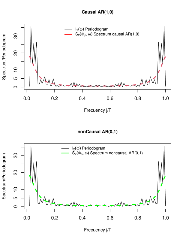
Figure 2: The top Figure is the periodogram and spectrum of a causal AR(1,0) $y_{t}=0.7y_{t-1}+\varepsilon_{t}$. The bottom Figure is the periodogram and spectrum of a noncausal AR(0,1) $y_{t}=0.7y_{t+1}+\epsilon_{t}$. $\varepsilon_{t}\sim$ alpha-stable $f_{a}(t;\alpha=1.5,\beta=0.25,\gamma=1,\delta=0)$, the sample size $T=100$.

2.3 Mixed Cuasal/noncausal MAR($r,s$)

Let $y_{t}$ be a mixed causal-noncausal autoregressive process MAR($r,s$) generated by

$$\varphi(L^{-1})\phi(L)y_{t}=\varepsilon_{t},$$ (26)

where $\phi(L)=1-\phi_{1}L-\phi_{2}L^{2}...\phi_{r}L^{r}$ corresponds to the causal component, and $\varphi(L^{-1})=1-\varphi_{1}L^{-1}-\varphi_{2}L^{-2}...\varphi_{s}L^{-s}$ to the noncausal. The traditional AR($p$) model is decomposed to the MAR($r,s$) model by the equivalence of its order $p=r+s$. The set of parameters is $\Upsilon_{r,s}=\left\{\phi_{1},...,\phi_{r},\varphi_{1},...,\varphi_{s}\right\}$. The MAR($r,s$) is a combination of the variable $y_{t}$ with $r$ lags and $s$ leads, and both polynomials $\varphi(z)$ and $\phi(z)$, with roots outside the unit circle. Alternatively, the polynomial $\varphi(z)$ has a causal representation with all its roots inside the unit circle, and the polynomial $\phi(z)$ outside the unit circle. For details, see K.-S. Lii and Rosenblatt (1996). Accordingly, $y_{t}$ has a two-sided moving average representation as in Equation 14. The polynomial of the MAR($r,s$) model is $\upsilon_{r,s}(z)=(1-\varphi_{1}z-\varphi_{2}z^{2}...-\varphi_{s}z^{s})(1-\phi_{1}z-\phi_{2}z^{2}...-\phi_{r}z^{r})$, this interaction between the components of the transfer function results in nonlinearities that can hinder the estimation of the parameters.

The MAR($r,s$) has a causal purely causal representation AR($r+s$,0), as follows

$$\upsilon^{*}_{r+s}(z)y_{t}=\xi^{*}_{t}.$$ (27)

This model representation can be found in Gourieroux and Jasiak (2018), Appendix A. Where $\xi^{*}_{t}=-1/\varphi_{s}\varepsilon_{t-s}$, and $\upsilon^{*}_{r+s}$ is the polynomial of the causal AR($r+s$,0) representation. To obtain it, we follow several steps. First, we apply distributive law for polynomial $\upsilon_{r,s}(L)$

$$\upsilon_{r,s}(L)=1-\varphi_{1}L^{-1}-\varphi_{1}L^{-2}-...-\varphi_{s}L^{-s}-\phi_{1}L+\phi_{1}\varphi_{1}+\phi_{1}\varphi_{2}L^{-1}+...+\phi_{1}\varphi_{s}L^{1-s}-\phi_{2}L^{2}+\phi_{2}\varphi_{1}L+\phi_{2}\varphi_{2}\\ +...+\phi_{2}\gamma_{s}L^{2-s}-\phi_{r}L^{r}+\phi_{r}\varphi_{1}L^{r-1}+\phi_{r}\varphi_{2}L^{r-2}+...+\phi_{r}\varphi_{s}L^{r-s}.$$

Reverting the process in $s$ time periods, or equivalently multiplying by $L^{s}$,

$$\upsilon_{r+s}(L)=-\varphi_{s}+\phi_{1}\varphi_{s}L+\phi_{2}\varphi_{s}L^{2}+...-\varphi_{2}L^{s-2}-\varphi_{1}L^{s-1}+\phi_{1}\varphi_{2}L^{s-1}+...+L^{s}+\phi_{1}\varphi_{1}L^{s}+\phi_{2}\varphi_{2}L^{s}+...-\phi_{1}L^{s+1}\\ +\phi_{2}\varphi_{1}L^{s+1}+...-\phi_{2}L^{s+2}+...+\phi_{r}\varphi_{s}L^{r}+...+\phi_{r}\varphi_{2}L^{r+s-2}+\phi_{r}\varphi_{1}L^{r+s-1}-\varphi_{r}L^{r+s}.\\$$

Solving for $y_{t}$, The closed form of the AR($r+s$,0) is

$$y_{t}=\varphi_{1}y_{t-1}+\varphi_{2}y_{t-2}+...-\frac{\varphi_{2}}{\varphi_{s}}y_{t-s+2}+\left(\frac{\phi_{1}\varphi_{2}-\varphi_{1}}{\varphi_{s}}\right)y_{t-s+1}+\left(\frac{1+\phi_{1}\varphi_{1}+\phi_{2}\varphi_{2}}{\varphi_{s}}\right)y_{t-s}+\left(\frac{\phi_{2}\varphi_{1}-\varphi_{1}}{\varphi_{s}}\right)y_{t-s-1}\\ -\frac{\phi_{2}}{\varphi_{s}}y_{t-s-2}+...+\phi_{r}y_{t-r}+...+\frac{\phi_{r}\varphi_{2}}{\varphi_{s}}y_{t-r-s+2}+\frac{\phi_{r}\varphi_{1}}{\varphi_{s}}y_{t-r-s+1}-\frac{\phi_{r}}{\varphi_{s}}y_{t-r-s}-\frac{\xi_{t-s}}{\varphi_{s}}.$$ (28)

The polynomial $\upsilon^{*}_{r+s}(z)$ , has the set of parameters $\Upsilon^{*}_{r+s}=\left\{\upsilon^{*}_{1},\upsilon^{*}_{2},...\upsilon^{*}_{s},...\upsilon^{*}_{r+s}\right\}$, then the AR($r+s$,0) can be written as

$$y_{t}=\upsilon^{*}_{1}y_{t-1}+\upsilon^{*}_{2}y_{t-2}+...+\upsilon^{*}_{s-2}y_{t-s+2}+\upsilon^{*}_{s-1}y_{t-s+1}+\upsilon^{*}_{s}y_{t-s}+\upsilon^{*}_{s+1}y_{t-s-1}+\upsilon^{*}_{s+2}y_{t-s-2}+...+\upsilon^{*}_{r}y_{t-r}\\ +...+\upsilon^{*}_{r+s-2}y_{t-r-s+2}+\upsilon^{*}_{r+s-1}y_{t-r-s+1}+\upsilon^{*}_{r+s}y_{t-r-s}+\xi^{*}_{t}.$$ (29)

Note that there is a one-to-one relation between Equations 26 and 29. Such representation becomes important in identifying the parameters by correctly selecting the initial values in the estimation. To shed light on this relation, we explore the transformation of the MAR($1,1$) into an AR($2,0$) in the Remark 2.

Remark 2. The MAR($1,1$) is represented by

$$(1-\varphi_{1}L^{-1})(1-\phi_{1}L)y_{t}=\varepsilon_{t}.$$ (30)

Multiplying by $L$ and solving for $y_{t}$, we obtain the AR($2,0$) representation

$$y_{t}=\left(\frac{1+\phi_{1}\varphi_{1}}{\varphi_{1}}\right)y_{t-1}-\frac{\phi_{1}}{\varphi_{1}}y_{t-2}-\frac{\varepsilon_{t-1}}{\varphi_{1}}.$$ (31)

The causal representation is

$$y_{t}=\upsilon^{*}_{1}y_{t-1}+\upsilon^{*}_{2}y_{t-2}+\xi^{*}_{t},$$ (32)

where the set of parameters is $\Upsilon^{*}=\left\{\upsilon^{*}_{1}=\frac{1+\phi_{1}\varphi_{1}}{\varphi_{1}},\upsilon^{*}_{2}=-\frac{\phi_{1}}{\varphi_{1}}\right\}$, and $\xi^{*}_{t}=-1/\varphi_{1}\varepsilon_{t-1}$. Estimating the set of parameters $\upsilon^{*}$ is not trivial, given the nonlinearity in the original model. For a similar representation of Equation 32, see Gourieroux and Jasiak (2018) proposition 3.1.

The spectrum of the MAR($r,s$) is

$$\begin{split}S_{2}(\Upsilon_{p,s},\omega)&=\frac{k_{2_{e}}}{2\pi}\frac{1}{\lvert\phi(z)\varphi(z^{-1})\rvert^{2}}\\ &=\frac{k_{2_{e}}}{2\pi}\frac{1}{\lvert(1-\phi_{1}z-\phi_{2}z^{2}...-\phi_{r}z^{r})(1-\varphi_{1}z^{-1}-\varphi_{2}z^{-2}...-\varphi_{s}z^{-s})\rvert^{2}}.\end{split}$$ (33)

The bispectrum is

$$\begin{split}S_{3}(\Upsilon_{r,s},\omega_{1},\omega_{2})&=\frac{k_{3_{e}}}{(2\pi)^{2}}\psi(\Upsilon_{r,s},\omega_{1})\psi(\Upsilon_{r,s},\omega_{2})\overline{\psi(\Upsilon_{r,s},\omega_{1}+\omega_{2})}.\end{split}$$ (34)

where $\psi(\Upsilon_{r,s},\omega)=1/\left[(1-\phi_{1}z-\phi_{2}z^{2}...-\phi_{r}z^{r})(1-\varphi_{1}z^{-1}-\varphi_{2}z^{-2}...-\varphi_{s}z^{-s})\right]$, and $\overline{\psi(\Upsilon_{r,s},-\omega_{1}-\omega_{2})}=1/\left[(1-\phi_{1}\overline{z}-\phi_{2}\overline{z}^{2}...-\phi_{r}\overline{z}^{r})(1-\varphi_{1}\overline{z}^{-1}-\varphi_{2}\overline{z}^{-2}...-\varphi_{s}\overline{z}^{-s})\right]$.

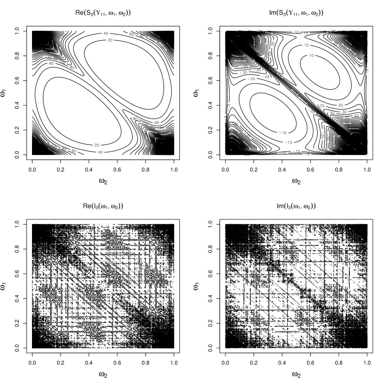
Figure 3: Real and Imaginary part of the bispectrum and biperiodogram for a MAR($1,1$) with $\phi_{1}=0.7$, $\varphi_{1}=0.2$, and the error term is alpha-stable $f_{a}(t;\alpha=1.5,\beta=0.25,\gamma=1,\delta=0)$, the sample size $T=200$.

In Figure 3, we show the real and imaginary parts of the bispectrum and the biperiodogram of simulated data from a MAR(1,1) with coefficients $\phi_{1}=0.7$ and $\varphi_{1}=0.2$ and $T=200$, the distribution of the errors is alpha-stable $f_{a}(t;\alpha=1.5,\beta=0.25,\gamma=1,\delta=0)$ with leptokurtic and skewness features. The set of frequencies $\omega_{1}$ is in the y-axis and $\omega_{2}$ in the x-axis. In this Figure, the white spaces indicate that the bispectrum value is relatively small and, therefore, the relation between the set of frequencies $\omega_{1}$ and $\omega_{2}$ is low. Conversely, when the Figure turns black, there is a higher relation between the set of frequencies. We can observe that the highest amount of information is stored in the low frequencies for $\omega_{1}$ and $\omega_{2}$, from 0 to 0.2 and 0.8 to 1 (see the symmetries in Equation 3). This accumulation of information fades as the frequency increases, from 0.2 to 0.5, and from 0.5 to 0.8. In addition, there is an accumulation of information on the $\omega_{1}=\omega_{2}$ diagonal that fades as it approaches the frequency 0.5. This same pattern can be seen in the periodogram and spectrum in Figure 2. Actually, the main diagonal of the biperiodogram (bispectrum) is equivalent to the periodogram (spectrum). Accordingly, the asymmetric patterns that arise from relations between frequencies outside the main diagonal are neglected in the second-order spectrum estimations, thus contributing to the correct estimation of the parameters and the identification of the model in the third-order estimation. Simultaneously, we can observe that the patterns present in the biperiodogram are replicated by the bispectrum. In the real part of the biperiodogram, we can observe two triangular patterns formed by relations between the high frequencies. One below the main diagonal at the frequencies 0.3 to 0.5 and another above the main diagonal at the frequencies 0.5 and 0.7. In addition, four triangular patterns formed a relationship between the high (low) frequencies of $\omega_{1}$ and low (high) frequencies of $\omega_{2}$. Two are below the main diagonal, and two are above the main diagonal. Additionally, in the imaginary part of the biperiodogram, there are two triangular patterns at low frequencies, one above and one below the main diagonal. In addition, there are four triangular patterns of the interaction between high frequencies and low frequencies, two above and two below the main diagonal.

3 Estimation

In this Section, we present the estimation function that was first proposed by Leonenko et al. (1998). However, we use the variation presented by Velasco and Lobato (2018) in terms of the scaling factor in the denominators of Equation 35. We define $\bm{\vartheta}$ as the set of parameters of the autoregressive model, for the causal $\bm{\vartheta}=\Phi_{r}$, for the noncausal $\bm{\vartheta}=\Phi_{s}$ and for the mixed $\bm{\vartheta}=\Upsilon_{r,s}$. We first perform a preliminary Gaussian likelihood estimation and obtain $\overline{\bm{\vartheta}}$, always assuming causality, and we evaluate it in the transfer functions $\psi(\overline{\bm{\vartheta}},\omega)$ and $\psi(\overline{\bm{\vartheta}},-\omega_{i}-\omega_{j})$ and the second order cumulant, $\overline{k}_{2}=2\pi T^{-1}\sum_{j=1}^{T-1}I_{2}(\omega_{j})/(\psi(\overline{\bm{\vartheta}},\omega_{j})\psi(\overline{\bm{\vartheta}},-\omega_{j}))$. This normalization by preliminary estimates has no effect on the identification of the parameters, given that they are invariant to any inversion of the polynomial roots. This step significantly simplifies the estimation compared with Leonenko et al. (1998). The estimation function is

$$R_{T}(\bm{\vartheta})=A_{2T}\sum_{j=1}^{T-1}\left(\frac{I_{2}(\omega_{j})-S^{*}_{2}(\bm{\vartheta},\omega_{j})}{\psi(\overline{\bm{\vartheta}},\omega_{j})\psi(\overline{\bm{\vartheta}},-\omega_{j})}\right)^{2}+A_{3T}\sum_{j=1}^{T-1}\sum_{i=1}^{T-1}\frac{\lvert I_{3}(\omega_{j},\omega_{i})-S^{*}_{3}(\bm{\vartheta},\omega_{j},\omega_{i})\rvert^{2}}{\psi(\overline{\bm{\vartheta}},\omega_{j})\psi(\overline{\bm{\vartheta}},\omega_{i})\psi(\overline{\bm{\vartheta}},-\omega_{j}-\omega_{i})},$$ (35)

where $A_{2T}=m(2\pi)^{2}/(4\overline{\kappa_{2}}^{2}T)$ and $A_{3T}=n(2\pi)^{4}/(6\overline{\kappa_{2}}^{3}T^{2})$. In all cases, $m=1-n$. The weights in our approach are arbitrarily set as $m=0.5$ and $n=0.5$. Terdik (1999) estimate an AR($1,0$) with different values for $m$, highlighting the efficiency gains with the correct selection. Nevertheless, in Velasco and Lobato (2018), the weights are optimally selected, increasing the efficiency, although they turn out to be unintuitive in some cases, increasing the complexity of the estimation. Considering theorem 2 in Velasco and Lobato (2018), we include in the spectrum and the bispectrum a consistent estimator of the standardized cumulants of orders two and three, respectively, that is

$$k^{*}_{2}(\bm{\vartheta})=\frac{2\pi}{T}\sum_{j=1}^{T-1}\frac{I_{2}(\omega_{j})}{\psi(\bm{\vartheta},\omega_{j})\psi(\bm{\vartheta},-\omega_{j})},\;\;\;\;\;\;k^{*}_{3}(\bm{\vartheta})=\frac{4\pi^{2}}{T^{2}}\sum_{j=1}^{T-1}\sum_{i=1}^{T-1}Re\left(\frac{I_{3}(\omega_{j},\omega_{i})}{\psi(\bm{\vartheta},\omega_{j})\psi(\bm{\vartheta},\omega_{i})\psi(\bm{\vartheta},-\omega_{j}-\omega_{i})}\right).$$ (36)

For a correct identification, the parameters and cumulants must be jointly estimated. Therefore, we modify the spectrum function to add the dependence of the cumulants to $\bm{\vartheta}$. The modified spectrum and bispectrum are

$$S^{*}_{2}(\bm{\vartheta},\omega_{j})=S_{2}(\bm{\vartheta},k^{*}_{2}(\bm{\vartheta}),\omega_{j}),\;\;\;S^{*}_{3}(\bm{\vartheta},\omega_{j},\omega_{i})=S_{3}(\bm{\vartheta},k^{*}_{3}(\bm{\vartheta}),\omega_{j},\omega_{i}).$$ (37)

When the data is Gaussian, the first term of the estimation function $R_{T}(\bm{\vartheta})$ (Equation 35) is sufficient to estimate and identify the autoregressive model correctly. The first term in $R_{T}(\bm{\vartheta})$ is equivalent to Whittle (1953) or Gaussian-likelihood. Nevertheless, when the data are non-Gaussian, Brillinger (1975) suggests including the second term, that is, the bispectrum estimation. This estimator is consistent and asymptotic normal. For details, see Terdik (1999); Velasco and Lobato (2018). The set of optimal parameters $\hat{\bm{\vartheta}}$ is obtained by minimizing $R_{T}$ by the quasi-Newton method

$$\hat{\bm{\vartheta}}=\operatorname*{arg\,min}_{\bm{\vartheta}\in\Theta}\>R_{T}(\bm{\vartheta}).$$ (38)

3.1 Consistency and asymptotic normality of $R_{T}(\bm{\vartheta})$

For the consistency of the estimator, we use Lemma 1 in Brillinger (1974), and Section 4.2, Theorem 73 in Terdik (1999). Let $\bm{\vartheta}$ be the true set of parameters, $\bm{\vartheta}\subset\Theta$, and

$$R(\bm{\vartheta})=m\int_{\Lambda_{1}}\left(\frac{I_{2}(\omega_{j})-S_{2}(\bm{\vartheta},\omega_{j})}{\psi(\overline{\bm{\vartheta}},\omega_{j})\psi(\overline{\bm{\vartheta}},-\omega_{j})}\right)^{2}d\omega_{j}+n\int\int_{\Lambda_{2}}\frac{\lvert I_{3}(\omega_{j},\omega_{i})-S_{3}(\bm{\vartheta},\omega_{j},\omega_{i})\rvert^{2}}{\psi(\overline{\bm{\vartheta}},\omega_{j})\psi(\overline{\bm{\vartheta}},\omega_{i})\psi(\overline{\bm{\vartheta}},-\omega_{j}-\omega_{i})}d\omega_{j}d\omega_{i}.$$ (39)

Theorem 1. Suppose that $y_{t}$ has a bispectrum $\lvert S_{3}(\omega_{j},\omega_{i})\rvert<\infty$. The first term in $R_{T}(\bm{\vartheta})$, $\left(\frac{I_{2}(\omega_{j})-S^{*}_{2}(\bm{\vartheta},\omega_{j})}{\psi(\overline{\bm{\vartheta}},\omega_{j})\psi(\overline{\bm{\vartheta}},-\omega_{j})}\right)^{2}$, belong to the finite union of closed intervals $\Lambda_{1}$, and the second term $\frac{\lvert I_{3}(\omega_{j},\omega_{i})-S^{*}_{3}(\bm{\vartheta},\omega_{j},\omega_{i})\rvert^{2}}{\psi(\overline{\bm{\vartheta}},\omega_{j})\psi(\overline{\bm{\vartheta}},\omega_{i})\psi(\overline{\bm{\vartheta}},-\omega_{j}-\omega_{i})}$ belong to the finite union of compact domains lying inside the open triangle of frequencies $\Lambda_{2}$. In addition, $R(\bm{\vartheta})$ has a unique minimum at $\bm{\vartheta}$. In this circumstances, $R_{T}(\bm{\vartheta})\overset{p}{\to}R(\bm{\vartheta})$ and $\hat{\bm{\vartheta}}\overset{p}{\to}\bm{\vartheta}$, as $T\rightarrow\infty$. $\hat{\bm{\vartheta}}$ is obtained minimizing $R_{T}(\bm{\vartheta})$.

Under the conditions mentioned above, and assuming that $\hat{\bm{\vartheta}}$ is close enough to $\bm{\vartheta}$ when $T\rightarrow\infty$, the Taylor expansion of $R_{T}(\hat{\bm{\vartheta}})$ is

$$\frac{\partial R_{T}(\hat{\bm{\vartheta}})}{\partial\bm{\vartheta}}=\frac{\partial R_{T}(\bm{\vartheta})}{\partial\bm{\vartheta}}+(\hat{\bm{\vartheta}}-\bm{\vartheta})\frac{\partial^{2}R_{T}(\hat{\bm{\vartheta}})}{\partial^{2}\bm{\vartheta}}.$$ (40)

As $\hat{\bm{\vartheta}}$ minimizes $R_{T}(\bm{\vartheta})$, $\frac{\partial R_{T}(\hat{\bm{\vartheta}})}{\partial\bm{\vartheta}}=0$. Then,

$$\hat{\bm{\vartheta}}-\bm{\vartheta}=-\frac{\frac{\partial R_{T}(\bm{\vartheta})}{\partial\bm{\vartheta}}}{\frac{\partial^{2}R_{T}(\hat{\bm{\vartheta}})}{\partial^{2}\bm{\vartheta}}}$$ (41)

Then

$$\hat{\bm{\vartheta}}=\bm{\vartheta}+o_{P}(1)$$ (42)

The closed forms for the first and second derivatives of Equation 41 are Terdik (1999) Section 4. It is reasonable to presume that the numerator in Equation 41 is zero since $\hat{\bm{\vartheta}}$ is close enough to $\bm{\vartheta}$, as the third-order cumulant is different from zero and the bispectrum exists.

Theorem 2. Under the fulfillment of Theorem 1, $\hat{\bm{\vartheta}}$ is asymptotically normal as $T\rightarrow\infty$

$$\sqrt{T}(\hat{\bm{\vartheta}}-\bm{\vartheta})\overset{D}{\to}N\left(0,\frac{\Sigma_{1}(\bm{\vartheta})}{\Sigma_{0}(\bm{\vartheta})}\right),$$ (43)

where $\Sigma_{0}(\bm{\vartheta})$ and $\Sigma_{1}(\bm{\vartheta})$ are Equations 4.17 and 4.18 in Terdik (1999). For the autoregressive process, the asymptotic variance of $\hat{\bm{\vartheta}}$ is

$$\begin{split}T\textrm{var}(\hat{\bm{\vartheta}}-\bm{\vartheta})&\approx\frac{\left(4m^{2}+\left[\frac{m^{2}}{4}\kappa+\frac{n^{2}}{2}+mn\right]\zeta^{2}\right)\eta}{\left(2m+\frac{n}{2}\zeta^{2}\right)^{2}\eta^{2}},\end{split}$$ (44)

where the skewness ($\zeta$) and kurtosis ($\kappa$) of the error sequence are defined by the standardized third and fourth-order cumulants as

$$\zeta=\frac{\textrm{Cum}(\varepsilon_{t},\varepsilon_{t},\varepsilon_{t})}{(\textrm{var}(\varepsilon_{t}))^{3/2}},\;\;and\;\;\kappa=\frac{\textrm{Cum}(\varepsilon_{t},\varepsilon_{t},\varepsilon_{t},\varepsilon_{t})}{(\textrm{var}(\varepsilon_{t}))^{2}}.$$ (45)

The parameter $\eta$ is the Integral respect to $\omega$ of the derivative of the modulus of the second-order transfer function with respect the set of parameters $\bm{\vartheta}$

$$\eta=\int_{0}^{1/2}\left(\frac{\partial\;}{\partial\bm{\vartheta}}log\;S_{2}(\omega,\bm{\vartheta})\right)^{2}d\omega=\int_{0}^{1}\frac{\frac{\partial}{\partial\bm{\vartheta}}\psi(\bm{\vartheta},\omega)}{\psi(\bm{\vartheta},\omega)}\frac{\frac{\partial}{\partial\bm{\vartheta}}\psi(\bm{\vartheta},-\omega)}{\psi(\bm{\vartheta},-\omega)}d\omega.$$ (46)

By solving Equation 44 we can obtain the standard errors. Notice that the asymptotic variance depends on the third and fourth-order cumulants. Since moments and cumulants do not exist for all distributions, we use their sample counterparts when they are absent. Lobato and Velasco (2022) developed closed formulas for the asymptotic variance of the ARMA model allowing for complex roots.

3.2 Estimation strategy

Theorem 1 shows that the correct set of parameters can be identified and consistently estimated by finding the global minimum of $R_{T}(\bm{\vartheta})$. However, this estimation function is not convex. On the contrary, it is multimodal, leading to the possibility of multiple local minima that increase as the number of parameters in the model grows. As a result, the empirical prerequisite for reaching the global minimum is the correct selection of the initial values, ensuring that $\hat{\bm{\vartheta}}$ is close enough to the true value $\bm{\vartheta}$. The latter entails certain limitations for noncausal and mixed models, given their nonlinearity and that $\bm{\vartheta}$ is not directly observable. Accordingly, the solution of this type of model is not unique and convergent. For a discussion of the multimodality in noncausal models, see Kindop (2021), and for mixed causal-noncausal, see Bec et al. (2020). To illustrate this situation, a model that is originally causal AR($2,0$) has three possible solutions for its parameters. A noncausal AR($0,2$), a mixed MAR($1,1$) and a causal AR($2,0$). Evidently, the solutions AR($0,2$) and MAR($1,1$) correspond to local minima of $R_{T}(\bm{\vartheta})$ since the global minimum must be for AR($2,0$).

The problem of identification in the noncausal model has been studied by Breid et al. (1991); Andrews et al. (2006); Lanne and Saikkonen (2011) in the time domain. In their procedure, they estimate assuming causality and select the order of the AR($p$). In a second step, they estimate the noncausal AR($0,s$) with $p=s$, and all possible combinations of mixed MAR($r,s$), with $r+s=p$, identifying as the appropriate model the one with the highest log-likelihood. Similarly, we propose an estimation strategy that significantly increases the probability of reaching the global minimum of the estimation function by selecting a set of initial parameters close enough to the true set of parameters, helping $\hat{\bm{\vartheta}}$ to converge in probability to $\bm{\vartheta}$. Then, we address the multimodality of the estimation function by selecting the model with the lowest $R_{T}(\hat{\bm{\vartheta}})$. The initial parameters are chosen based on the pure causal representation of the noncausal (Equation 21) and mixed models (Equation 27) from which their original roots can be reconstructed. In this context, we developed a tool to identify purely causal, noncausal, and mixed autoregressive models in the frequency domain.

For clarity, $R_{T}(\Phi_{r})$ refers to the estimation function when the model is purely causal AR($r$,0), $R_{T}(\Phi_{s})$ when the model is purely noncausal AR(0,$s$), and $R_{T}(\Upsilon_{r,s})$ when is mixed causal-noncausal MAR($r,s$). As a common first step, we perform Gaussian likelihood or Whittle estimation and obtain $\overline{\bm{\vartheta}}$ and $\overline{k}_{2}$.

1. For the estimation of the Causal AR($r,0$), the selection of the initial values to minimize $R_{T}(\Phi_{r})$ is $\overline{\bm{\vartheta}}$, that is

   $$\Phi_{p_{0}}=\overline{\bm{\vartheta}}=\left\{\phi_{1_{0}},\phi_{2_{0}},...,\phi_{p_{0}}\right\}.$$ (47)

   The initial values are always obtained in the preliminary estimation, assuming causality. The minimum obtained by the estimation function is $R_{T}(\hat{\Phi}_{r})$.

2. For the estimation of the noncausal AR($0,s$), the selection of the initial values to minimize $R_{T}(\Phi_{s})$ are the coefficients from the polynomial $\varphi^{*}(z)$ in Equation 20, that its causal representation in Equation 21

   $$\Phi_{s_{0}}=\left\{\varphi^{*}_{1},\varphi^{*}_{2},...,\varphi^{*}_{s}\right\}.$$ (48)

   We highlight that in Gourieroux and Jasiak (2018), it is shown that Gaussian-likelihood estimation is a consistent estimator of the causal representation of a noncausal model. After the estimation, the set of parameters $\Phi_{s}$ is reconstructed with Equation 20. The minimum obtained by the estimation function is $R_{T}(\hat{\phi}_{s})$.

   Example 1 We want to estimate the noncausal AR($0,2$) $y_{t}=\varphi_{1}y_{t+1}+\varphi_{2}y_{t+2}+\varepsilon_{t}$, the steps are

   1. Estimate the causal AR($2,0$) by Gaussian likelihood, obtain $\hat{\varphi}^{*}_{1}$ and $\hat{\varphi}^{*}_{2}$.

   2. Optimize $R_{T}(\Phi_{s})$ with the initial parameters $\Phi_{s_{0}}=\left\{\hat{\varphi}^{*}_{1},\hat{\varphi}^{*}_{2}\right\}$.

   3. Recover $\hat{\Phi}_{s}$ as $\hat{\varphi}_{1}=-\frac{\hat{\varphi}^{*}_{1}}{\hat{\varphi}^{*}_{2}}$, $\hat{\varphi}_{2}=\frac{1}{\hat{\varphi}^{*}_{2}}$.

3. For the estimation of the mixed MAR($r,s$) the selection of the initial values to minimize $R_{T}(\Upsilon_{r,s})$ are the set of parameters

   $$\Upsilon_{r_{0}+s_{0}}=\left\{\phi_{1_{0}},...,\phi_{r_{0}},\varphi_{1_{0}},...,\varphi_{s_{0}}\right\}.$$ (49)

   We must first conduct a Gaussian-likelihood to obtain the initial values and obtain $\overline{\bm{\vartheta}}$. After, the set of parameters $\Upsilon_{r,s}$ is reconstructed using the relation between Equations 28 and 29.

   Example 2 We want to estimate a mixed causal-noncausal MAR($1,1$), the steps are

   1. Estimate the causal AR($2,0$) by Gaussian likelihood, and obtain $\hat{\upsilon}^{*}_{1}$ and $\hat{\upsilon}^{*}_{2}$.

   2. Recover $\hat{\Upsilon}_{1,1}$ as $\hat{\upsilon}^{*}_{1}=\frac{1+\phi_{1}\varphi_{1}}{\varphi_{1}}$, and $\hat{\upsilon}^{*}_{2}=-\frac{\phi_{1}}{\varphi_{1}}$. Notice that this nonlinear system has two possible solutions. Both with possible complex roots.

      $$\phi_{1_{0}}=\frac{1}{2}\left(\hat{\upsilon}^{*}_{1}-\sqrt{(\hat{\upsilon}^{*}_{1})^{2}+4\hat{\upsilon}^{*}_{2}}\right),\;\textrm{and}\;\;\;\varphi_{1_{0}}=\frac{-\hat{\upsilon}^{*}_{1}+\sqrt{(\hat{\upsilon}^{*}_{1})^{2}+4\hat{\upsilon}^{*}_{2}}}{2\hat{\upsilon}^{*}_{2}},$$

      $$\phi_{1_{0}}=\frac{1}{2}\left(\hat{\upsilon}^{*}_{1}+\sqrt{(\hat{\upsilon}^{*}_{1})^{2}+4\hat{\upsilon}^{*}_{2}}\;\right),\;\textrm{and}\;\;\;\varphi_{1_{0}}=-\frac{\hat{\upsilon}^{*}_{1}+\sqrt{(\hat{\upsilon}^{*}_{1})^{2}+4\hat{\upsilon}^{*}_{2}}}{2\hat{\upsilon}^{*}_{2}}.$$

   3. Optimize $R_{T}(\Upsilon_{r,s})$ with initial parameters $\Upsilon_{1,1}=\left\{\phi_{1_{0}},\varphi_{1_{0}}\right\}$.

   4. Obtain $\hat{\Upsilon}_{1,1}=\left\{\hat{\phi}_{1},\hat{\varphi}_{1}\right\}$.

After the estimation, we proceed with the model identification based on the value of the estimation function.

1. If the model is causal, then $R_{T}(\hat{\Phi}_{r})=\textrm{min}\left\{R_{T}(\hat{\Phi}_{r}),R_{T}(\hat{\Phi}_{s}),R_{T}(\hat{\Upsilon}_{r,s})\right\}$.

2. If the model is noncausal, then $R_{T}(\hat{\Phi}_{s})=\textrm{min}\left\{R_{T}(\hat{\Phi}_{r}),R_{T}(\hat{\Phi}_{s}),R_{T}(\hat{\Upsilon}_{r,s})\right\}$.

3. If the model is mixed causal-noncausal, then $R_{T}(\hat{\Upsilon}_{r,s})=\textrm{min}\left\{R_{T}(\hat{\Phi}_{r}),R_{T}(\hat{\Phi}_{s}),R_{T}(\hat{\Upsilon}_{r,s})\right\}$.

4 Simulation study

We perform an extensive Monte Carlo study to investigate the finite sample properties of our estimation strategy using $R_{T}(\bm{\vartheta})$. We consider the ability to identify the three types of models, causal, noncausal and mixed. The results are based on M=1000 simulations. We use the alpha-stable distribution as the data-generating process (DGP). For implementations of the alpha-stable distribution in noncausal models, see Fries and Zakoian (2019) and Fries (2021). The probability density function of the alpha-stable is

$$f_{a}(t;\alpha,\beta,\gamma,\delta)=exp(it\delta-\lvert\gamma t\rvert^{\alpha}(1-i\beta sgn(t)(\lvert\gamma t\rvert^{1-\alpha}-1)tan(\pi\alpha 2^{-1}))),$$ (50)

where $\alpha\in(0,2)$ is the stability parameter, $\beta\left[-1,1\right]$ the skewness parameter, $\gamma>0$ the scale parameter, and $\delta\in\Re$ the location parameter. We generate random numbers with length $T=\left\{100,200,500\right\}$, for the parameters we choose $\alpha=\left\{1.5,1.8\right\}$, $\beta=0.25$, $\gamma=1$ and $\delta=0$. To allow for skewness and leptokurticity. In Figure 4, we show an alpha-stable MAR($1,1$), the empirical density, the ACF, and the PACF. We can observe asymmetric cycles, bubble patterns, and high persistence in the ACF. Since we are interested in the ability of our method to identify the correct model, we consider three DGPs, a purely causal AR($2,0$), with $\phi_{1}=0.7,\phi_{2}=0.2$, a purely noncausal AR($0,2$), with $\varphi_{1}=0.7,\varphi_{2}=0.2$, and a mixed MAR($1,1$) with $\phi_{1}=0.7,\varphi_{1}=0.2$.

In Table 1, we present the percentage with which we identify the correct model (identification rate) for the estimation of $R_{T}(\bm{\vartheta})$. In the first column, there are the parameters of the alpha-stable distribution, notice that the only parameter that varies is $\alpha$. The second column is the sample size $T$. To compare our method of selecting the initial values and their impact on the identification rate, we compare it with the second-order method, i.e., selecting the initial values directly from the AR($2,0$) Gaussian likelihood. A similar procedure is used in the MARX package Hecq, Lieb, and Telg (2017). The identification rate is the number of times that the method succeeds in detecting that the model is causal AR($2,0$) when the DGP is AR($2,0$), given the three possibilities, causal AR($2,0$), noncausal AR($0,2$), and mixed MAR($1,1$). The same logic follows when the DGP is noncausal AR($0,2$) and mixed MAR($1,1$). We report the identification rate for the causal AR($2,0$) in the third column, in the fourth column for the AR($0,2$), and in the fifth column for the MAR($1,1$).

Table 1: Rate of Identification of $R_{T}(\bm{\vartheta})$

		AR($2,0$)		MAR($1,1$)		AR($0,2$)
		$\phi_{1}=0.7,\;\phi_{2}=0.2$		$\phi_{1}=0.7,\;\varphi_{1}=0.2$		$\varphi_{1}=0.7,\;\varphi_{2}=0.2$
alpha-Stable dist	T	Initial values with our method	Initial values from AR(2)	Initial values with our method	Initial values from AR(2)	Initial values with our method	Initial values from AR(2)
$\alpha=1.5$	100	74%	74%	72%	42%	76%	10%
	200	94%	94%	80%	60%	82%	18%
	500	95%	95%	84%	66%	86%	21%
$\alpha=1.8$	100	72%	72%	53%	39%	64%	6%
	200	79%	79%	61%	44%	72%	14%
	500	88%	88%	69%	47%	74%	18%

The identification rate reveals that even with 100 observations, our strategy performs well for all three models. In all cases, the percentage increases as the number of data increases. The model with the highest level of identification is the causal AR($2,0$), followed by the mixed MAR($1,1$) and the noncausal AR($0,2$). As was expected, the more leptokurtic distribution, $\alpha=1.5$, has a higher identification rate since it deviates more from the Gaussian distribution. The results are equivalent in other simulations with different parameters (not presented). However, the identification rate decays slightly as the parameters approach the unit circle. In the case of the parameters taken from the coefficients of the AR($2,0$) model estimation by Gaussian-likelihood, the identification decreases significantly. In this case, the identification is lower in the noncausal AR($0,2$) model than in the mixed MAR($1,1$) model. It is noteworthy that identification is possible when the sample moments of the data exist, even knowing that for the alpha-stable distribution, only the moments of orders two, three, and four exist when $\alpha=2$.

The mean and standard deviation of the estimated parameters are reported in Table 2, (we only show the results for our estimation strategy).

Table 2: Mean and Standard Deviation

		Causal AR(2)				noncausal AR(2)				MAR($1,1$)
alpha-Stable dist		$\phi_{1}=0.7$		$\phi_{2}=0.2$		$\varphi_{1}=0.7$		$\varphi_{2}=0.2$		$\phi_{1}=0.7$		$\varphi_{1}=0.2$
	T	Mean	St.dev	Mean	St.dev	Mean	St.dev	Mean	St.dev	Mean	St.dev	Mean	St.dev
$\alpha=1.5$	100	0.733	0.112	0.147	0.127	0.702	0.097	0.155	0.112	0.667	0.162	0.211	0.147
	200	0.703	0.099	0.188	0.095	0.697	0.096	0.183	0.089	0.697	0.054	0.207	0.089
	500	0.700	0.055	0.196	0.058	0.700	0.062	0.195	0.060	0.701	0.031	0.200	0.042
$\alpha=1.8$	100	0.734	0.154	0.136	0.157	0.744	0.106	0.166	0.130	0.621	0.211	0.257	0.202
	200	0.727	0.091	0.170	0.110	0.731	0.090	0.157	0.091	0.699	0.077	0.191	0.105
	500	0.705	0.071	0.182	0.079	0.682	0.066	0.214	0.065	0.692	0.076	0.204	0.095

In all three cases, the mean of the estimated parameters is near the true parameters, showing that the estimation is unbiased and revealing the merits of our estimation strategy. The results are better for the more leptokurtic distribution, $\alpha=1.5$, in all cases, meaning that the estimator decreases in bias as the data deviates from normality. As is expected from Theorem 1, the results improve as $T$ increases. In parallel, the standard deviation decreases as $T$ increases. For the causal and noncausal models, the second parameter deviates slightly from its original value when the sample is 100 and 200. The problem is corrected when the sample is 500. In all cases, its standard deviation is lower than the other distribution $\alpha=1.8$, revealing that the variance of the estimator depends on the sample moments.

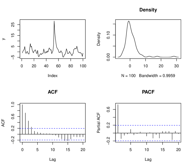
Figure 4: MAR($1,1$) with $\phi_{1}=0.7$ and $\varphi_{1}=0.2$, with errors alpha-stable $f_{a}(t;\alpha=1.5,\beta=0.25,\gamma=1,\delta=0)$, $T=100$.

5 Empirical application

For applying the models discussed above and our estimation strategy, we considered eight monthly commodity prices, including Cotton, measured in US cents per pound. Wheat, Barley, Zinc, Copper, Aluminium, and Nickel, are measured in US dollars per metric ton. We also consider the Brent oil, measured in US dollars per barrel. The eight series are from January 1900 through July 2022 for 383 observations. The data was obtained from the FRED (https://fred.stlouisfed.org/).

An accurate understanding of the dynamics of commodity prices is critical to setting the macroeconomic strategies of exporting and importing countries. In many of them, the stability of their national accounts depends on their behavior. The factors that affect commodity prices are the climate, geopolitical events, the internal policies of each country, transport costs, demand, supply, and profitability, among others. Although commodities are a competitive market with many buyers and sellers, there is evidence that their dynamics can be explained with noncausal autoregressive models. Hecq and Voisin (2021) found evidence of noncausality in monthly Nickel prices, Hecq and Voisin (2019); Gourieroux et al. (2021) in crude oil monthly prices, Karapanagiotidis (2014) in 25 commodity futures price, including soft, precious metals, energy, and livestock sectors and Lof and Nyberg (2017) in the exchange rates of commodity exporters.

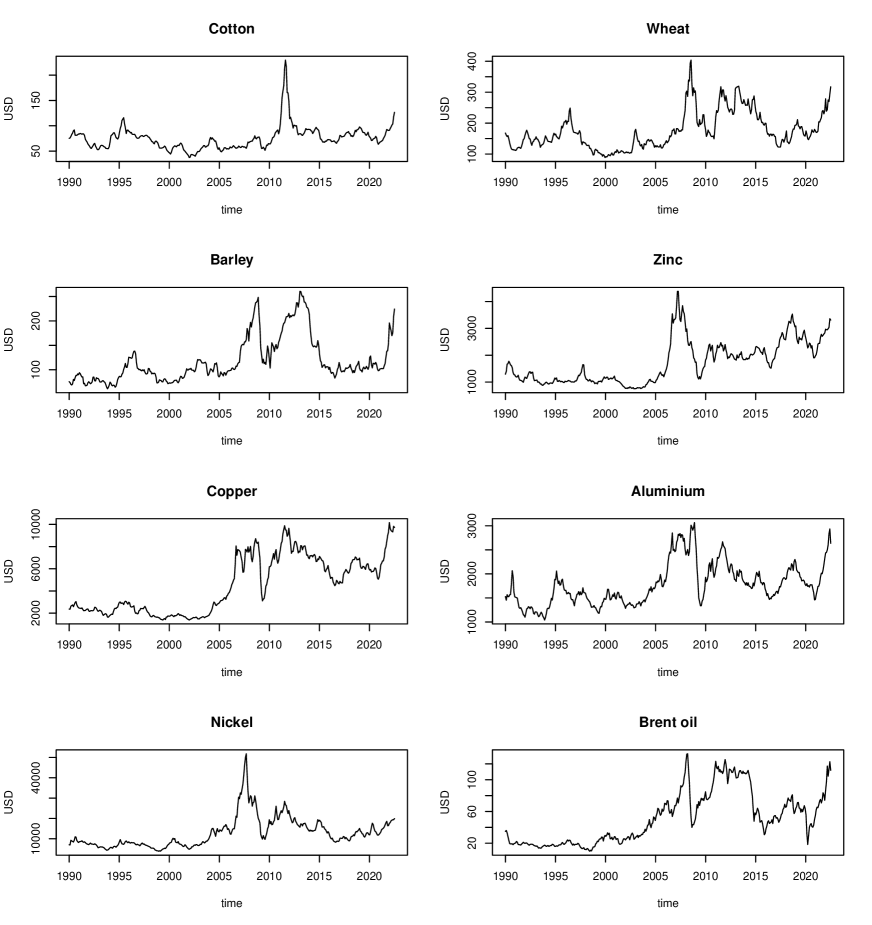
Figure 7: Prices of the eight commodities

All series do not share the same trend, but they appear to be affected by similar shocks. We can observe in Figure 7 peaks during the 2008 financial crisis, then a drop around 2010 and a subsequent increase from late 2010 to early 2014, then generalized increases in 2022 due to the recent Russian invasion of Ukraine. For the eight series, the null hypothesis of unit root is not rejected in the Augmented Dickey-Fuller test with constant and trend alternatives.

As the data seems non-stationary, a transformation is necessary for the estimation. For instance, Hencic and Gouriéroux (2015) use a cubic trend, Fries and Zakoian (2019) use a linear trend or a simple centering, Hecq et al. (2020); Cubadda et al. (2019) use the returns, Hecq, Telg, and Lieb (2017) use the X-11 method to filtering the seasonal effects. However, arbitrarily selecting the type of trend or the transformation of the data can affect the dynamics of the series, greatly influencing the noncausal component. Alternatively, Hecq and Voisin (2019) proposes to use the Hodrick-Prescott (HP hereafter) filter with a penalty parameter $\lambda=$129.600 for monthly data, indicating through a Monte Carlo study that the method keeps the data dynamics unaltered. Notwithstanding the above, there are criticisms about the dynamics induced by the HP filter and the selection of its penalty parameter; see Hamilton (2018) for details. For the sake of discussion, we consider two transformations, the HP filter with a penalty parameter $\lambda=129.600$, using the cyclical component, and the logarithmic returns. The Figures of these two transformations are respectively 8, 9.

Following Breid et al. (1991), we estimate all series by Gaussian likelihood and selected the order $p$ by second-order information criteria, AIC and BIC. After selecting the order, we fit the AR($p$) model and obtain the residuals. The descriptive statistics, the selected $p$, and the p-value of the Ljung-Box test for the residuals are in Table 3.

Table 3: Descriptive statistics and Ljung-Box p-value for the selected AR($p$)

	Cyclical component HP filter
	Descriptive Statistics				Selected $p$	Residuals AR($p$) Ljung-Box p-value
	Mean	Std.Dev	Skewness	Kurtosis		Lag-1	Lag-2
Cotton	7.6E-16	17.20	3.37	21.99	2	1.000	0.454
Wheat	-4.3E-15	34.72	1.17	6.95	2	0.172	0.225
Barley	1.4E-15	24.94	0.83	4.33	2	0.156	0.224
Zinc	-2.5E-14	423.35	1.34	7.94	2	0.344	0.144
Copper	-1.4E-13	889.27	-0.39	6.08	2	0.273	0.462
Aluminium	-5.5E-15	262.35	-0.01	4.31	2	0.042	0.121
Nickel	-3.3E-13	4151.15	2.13	16.77	2	0.513	0.733
Brent oil	1.1E-15	13.65	0.05	4.93	2	0.660	0.600
Log-returns
	Descriptive Statistics				Selected $p$	Residuals AR($p$) Ljung-Box p-value
	Mean	Std.Dev	Skewness	Kurtosis		Lag-1	Lag-2
Cotton	0.001	0.055	-0.334	6.552	1	0.262	0.204
Wheat	0.002	0.067	0.065	4.514	1	0.736	0.630
Barley	0.003	0.061	-0.113	5.371	2	0.443	0.324
Zinc	0.002	0.061	-0.450	5.157	2	0.549	0.483
Copper	0.004	0.061	-0.593	7.810	1	0.953	0.919
Aluminium	0.001	0.048	-0.353	4.533	1	0.367	0.521
Nickel	0.003	0.079	-0.111	4.412	2	0.853	0.957
Brent oil	0.003	0.099	-0.983	8.956	2	0.870	0.615

The series are not non-Gaussian for both transformations. This result was corroborated by the Jarque-Bera test (not presented). In the HP transformation, the highest standard deviations are for Nickel and Copper. All the series have a positive skewness except for Copper and Aluminium. Cotton and Nickel are the series with the highest kurtosis. The selected order is $p=2$ in all cases. We construct the residuals for the AR($2$) model and calculate the Ljung-Box test; the p-value for the first two lags is reported. For all the cases, the null hypothesis is not rejected.

For the log returns, the standard deviation is relatively similar for all cases, with Brent and Nickel having the highest values. All the series have negative skewness except for Wheat. All series are leptokurtic, with the highest kurtosis for Brent and Copper. In four cases, the selected order $p=1$, and in four cases, $p=2$. The AR($p$) model residuals are calculated, and we report the p-value of the first two lags of the Ljung-Box test. For all the cases, the null hypothesis is not rejected. For the cyclical component of the HP filter, the competing models are the AR($2,0$), the MAR($1,1$), and the AR($0,2$). In Table 4, we report the estimation using $R_{T}(\bm{\vartheta})$ of the three models. The standard deviation of the coefficients is in parentheses. We also present the residual sum of squares (SSE) and the value of the estimation function for each model.

Table 4: Estimation of $R_{T}(\bm{\vartheta})$ for the HP cyclical component

		Commodity
Model		Cotton	Wheat	Barley	Zinc	Copper	Aluminium	Nickel	Brent oil
AR($2,0$)	$\phi_{1}$	1.375 (0.066)	1.120 (0.040)	1.227 (0.045)	1.332 (0.059)	1.319 (0.058)	1.319 (0.058)	1.372 (0.066)	1.282 (0.050)
	$\phi_{2}$	-0.463 (0.045)	-0.307 (0.049)	-0.308 (0.049)	-0.404 (0.046)	-0.417 (0.046)	-0.412 (0.047)	-0.457 (0.045)	-0.386 (0.045)
	SSE	8945.5	67963	20057	6193530	32314949	2859360	596755528	8479.296
	$R_{T}(\hat{\Phi}_{p})$	33.457	32.978	32.563	35.435	33.037	33.337	33.538	35.808
MAR($1,1$)	$\phi_{1}$	0.496 (0.045)	0.423 (0.046)	0.319 (0.048)	0.484 (0.044)	0.472 (0.045)	0.511 (0.044)	0.564 (0.042)	0.459 (0.043)
	$\varphi_{1}$	0.844 (0.027)	0.810 (0.030)	0.880 (0.024)	0.859 (0.026)	0.820 (0.029)	0.810 (0.030)	0.813 (0.030)	0.811 (0.029)
	SSE	9022.2	68549.9	20034	6215542	32148623	2800194	596483019	8329.35
	$R_{T}(\hat{\Upsilon}_{p,s})$	32.956	32.898	32.415	35.163	32.944	33.241	33.084	35.755
AR($0,2$)	$\varphi_{1}$	1.317 (0.058)	1.199 (0.041)	1.055 (0.018)	1.332 (0.059)	1.312 (0.057)	1.315 (0.057)	1.378 (0.067)	1.293 (0.052)
	$\varphi_{2}$	-0.416 (0.047)	-0.308 (0.049)	-0.143 (0.051)	-0.404 (0.046)	-0.409 (0.047)	-0.408 (0.047)	-0.463 (0.045)	-0.398 (0.045)
	SSE	9078.3	67759.8	20943	5823797	32116060	2790389	596800743	8340.1
	$R_{T}(\hat{\Phi}_{s})$	31.720	32.984	32.474	35.381	33.054	33.331	33.391	35.795
Selected model		AR($0,2$)	MAR($1,1$)	MAR($1,1$)	MAR($1,1$)	MAR($1,1$)	MAR($1,1$)	MAR($1,1$)	MAR($1,1$)
Selected model by MLE with MARX		AR($0,2$)	AR($2,0$)	MAR($1,1$)	MAR($1,1$)	MAR($1,1$)	AR($0,2$)	MAR($1,1$)	AR($0,2$)

The results from Table 4 reveal that the model selected in seven cases is MAR($1,1$), except for Cotton, which is a purely noncausal AR($0,2$). A feature of the causal AR($2,0$) estimation is that the coefficient of the first lag is outside the unit circle, and the second lag is negative and inside the unit circle. This result is equivalent in the noncausal model AR($0,2$), with the coefficient of the first lead outside the unit circle and the coefficient of the second lead, negative and inside the unit circle. Notice that the coefficient outside the unit circle does not violate the stationarity assumption since, in all cases, the modulus of the characteristic roots is greater than one. Gaussian-likelihood also obtains this estimation pattern. Alternatively, for the MAR($1,1$), the noncausal coefficient is greater than the causal coefficient, both positive and significant. The causal coefficient is between 0.319 for Barley and 0.564 for Nickel. The noncausal coefficient is more homogeneous and always positive, between 0.810 for Aluminium and 0.880 for Barley. In most cases, the AR($2,0$) model has the lower SSE. In the last row, we add the estimation using the MARX package Hecq, Lieb, and Telg (2017), that is, Student’s t MLE. The results are equivalent in 5 cases. However, different for Wheat AR($2,0$), Aluminium AR($0,2$), and Brent oil AR($0,2$). Similar identification and coefficients were obtained following the time domain estimation of Lanne and Saikkonen (2011). In Table 5, we present the estimation using $R_{T}(\bm{\vartheta})$ for the log-returns.

Table 5: Estimation Log-returns

		Commodity
Model		Cotton	Wheat	Barley	Zinc	Copper	Aluminium	Nickel	Brent oil
AR($p$,0)	$\phi_{1}$	0.415 (0.084)	0.207 (0.062)	0.370 (0.057)	0.268 (0.016)	0.401 (0.087)	0.332 (0.089)	0.327 (0.043)	0.308 (0.048)
	$\phi_{2}$			-0.184 (0.060)	0.041 (0.016)			-0.031 (0.045)	-0.193 (0.050)
	SSE	0.920	1.616	1.230	1.320	1.192	0.825	2.028	3.852
	$R_{T}(\hat{\Phi}_{p})$	31.924	31.741	32.166	32.529	31.413	31.528	32.076	35.574
MAR($1,1$)	$\phi_{1}$			-0.085 (0.051)	0.333 (0.019)			0.293 (0.054)	-0.146 (0.010)
	$\varphi_{1}$			0.352 (0.048)	-0.090 (0.054)			0.021 (0.057)	0.440 (0.028)
	SSE			1.265	1.291			2.031	3.986
	$R_{T}(\hat{\Upsilon}_{p,s})$			32.169	32.554			32.077	35.479
AR(0,$s$)	$\varphi_{1}$	0.378 (0.111)	0.224 (0.073)	0.378 (0.033)	0.164 (0.010)	0.383 (0.066)	0.279 (0.066)	0.321 (0.052)	0.474 (0.022)
	$\varphi_{2}$			-0.144 (0.035)	0.073 (0.011)			-0.032	-0.113 (0.061)
	SSE	0.920	1.612	1.225	1.309	1.192	0.814	2.030	3.937
	$R_{T}(\hat{\Phi}_{s})$	31.870	31.739	32.162	32.527	31.430	31.539	32.077	35.486
Selected model		AR(0,1)	AR(0,1)	AR($0,2$)	MAR($1,1$)	AR(1,0)	AR(1,0)	MAR($1,1$)	MAR($1,1$)
Selected model by MLE with MARX		AR(0,1)	AR(0,1)	AR($0,2$)	MAR($1,1$)	AR(1,0)	AR(0,1)	AR($2,0$)	AR($0,2$)

We identify an AR(1,0) for Cotton and Wheat, AR(0,1) for Copper and Aluminium, one AR($0,2$) for Barley, and three MAR($1,1$) for Zinc, Nickel, and Brent oil. In the case of the AR(0,1) model, the coefficients are 0.415 for Cotton and 0.207 for Wheat. Both are highly significant. Similar results are obtained for the AR(1,0) model, where the coefficients are 0.383 for Copper and 0.279 for Aluminium. For MAR($1,1$), the causal coefficients are 0.333 and 0.293, and -0.146 for Zinc, Nickel, and Brent oil, respectively. For the same commodities, the noncausal coefficients are -0.090, 0.021, and 0.440, respectively. In the last row, we add the identification of the MARX package using the ’s t MLE. The results are equivalent in six cases. they are different for Aluminium AR(0,1) and Brent oil AR($0,2$).

It is noted that the possible dynamics found in the data are dependent on the transformation performed. In the case of the HP filter, in seven of the eight possible cases, the model identified in its cyclical component is MAR($1,1$). On the other hand, the log-return transformation results are more heterogeneous, with three MAR($1,1$), two AR($0,1$), one AR($0,2$), and one AR($1,0$). The results are similar using Student’s t MLE using the MARX package. In the case of the HP filter, the identification is equivalent in five cases. In the case of the log returns, it is equivalent in six cases.

The real and imaginary parts of the bispectrum and the biperiodogram of the MAR($1,1$) for the Brent oil cyclical component are presented in Figure 5. We observed that the highest value relations are found between the low frequencies, 0 to 0.25 and 0.8 to 1. In this range, we observe asymmetric relations, reflecting the non-Gaussianity of the data. No clear relations are observed between the middle frequencies, from 0.25 to 0.4, and the low frequencies. Neither between the high frequencies, from 0.4 to 0.5, with the low frequencies. The same pattern can be observed in the main diagonal of the real and imaginary parts of the biperiodogram.

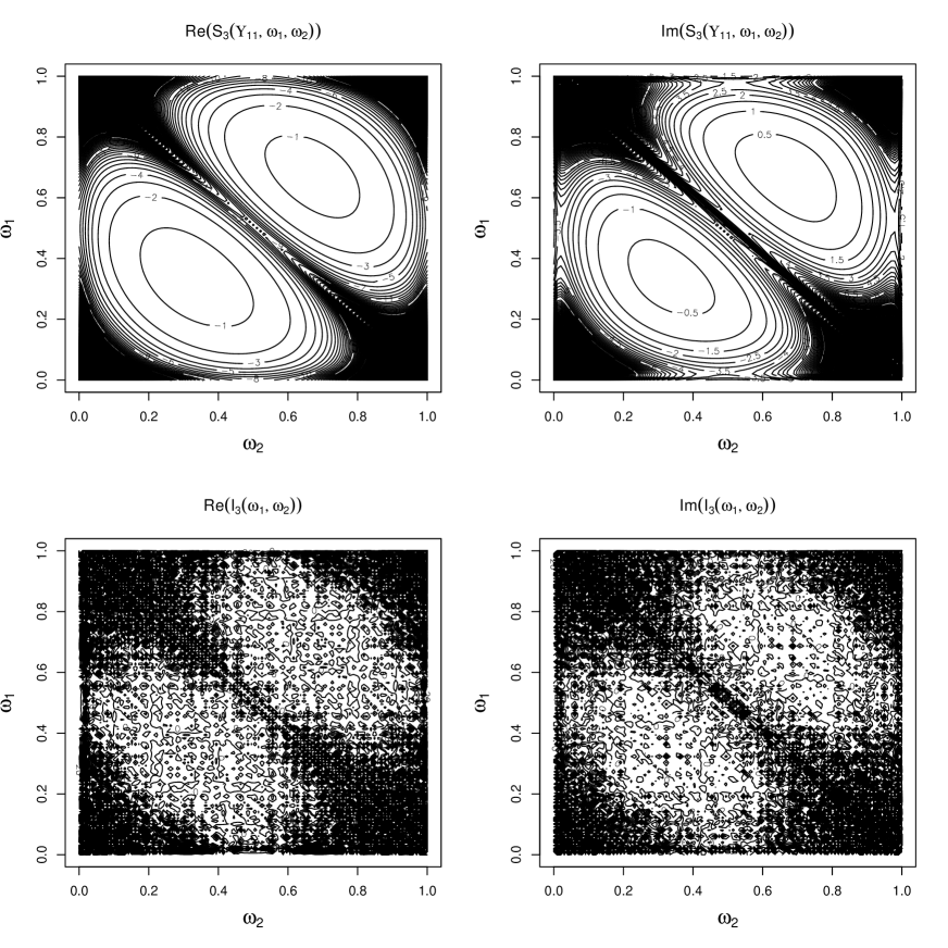
Figure 5: MAR($1,1$) Real and imaginary part of the bispectrum and biperiodogram for the cyclical component of the Brent oil

In Figure 6, we present the graphical representation of the estimation function $R_{T}(\hat{\Upsilon}_{p,s})$ for the cyclical component of the Brent oil. On the x-axis is the noncausal coefficient ($\varphi_{1}$), and on the y-axis is the causal coefficient ($\phi_{1}$). The surface features have been truncated to accentuate the areas where the minima are located. We observe three regions where minima occur. Two of them correspond to local minima, one for the causal model AR(2,0) and one for the noncausal AR(0,2). The global minimum of the estimation function is for the MAR(1,1) with parameters $\varphi_{1}=0.811$ and $\phi_{1}=0.459$, located at the intersection of the vertical (green) and horizontal (red) lines.

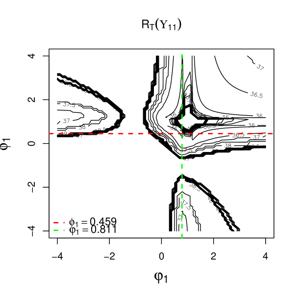
Figure 6: Brent oil MAR($1,1$) cyclical component, estimation function $R_{T}(\hat{\Upsilon}_{r,s})$

6 Conclusions and Discussion

This paper presents a frequency domain estimation method based on a combination of the spectrum and the bispectrum for causal, noncausal, and mixed autoregressive models. We test its properties in finite samples by conducting a Monte Carlo study, finding unbiased estimated parameters and asymptotic normality in the variance. We also performed an empirical application on eight monthly commodity prices finding evidence of noncausality and mixed causality/noncausality.

Our contribution to the current literature is divided into three parts. First, we develop a general scheme for selecting the initial values for the estimation of noncausal and mixed causal-noncausal based on their causal representations. In our second contribution, we present a decision method for identifying the model based on the existence of the global minimum in the estimation function. Third, we propose the third-order spectral estimation of mixed models.

Our estimation method is consistent with strong asymptotic properties without assuming any probability density function. Instead, non-Gaussianity is required. Nonetheless, it may have a higher computational burden than parametric methods, which assume a distribution function to estimate by ML. Although our method is helpful for estimating causal, noncausal, and mixed models, it depends on the initial values obtained in second-order estimates.

The dynamics of commodities depend on their past history but also show a dependence on future information. Nevertheless, the possible dynamics depend on the transformation performed. In the case of the HP filter, the model identified is a MAR($1,1$) in seven cases. On the other hand, in the log-return transformation, the results are more heterogeneous. It identifies an AR($1,0$) twice, AR($0,1$) twice, one AR($0,2$) and three MAR($1,1$). The dynamics are stronger in the HP filter.

Developing a tool to detect dynamics considering higher-order cumulants is interesting for future research. This is because although the estimation is of third-order, second-order criteria are used to detect dynamics, leading to a process that may not reveal all the information in the data. Also consider the existence of the noninvertible component of the moving average model.

Appendix 1. Figures

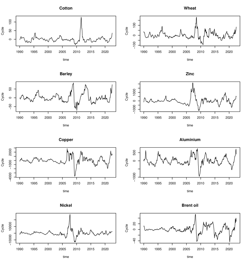
Figure 8: HP cyclical component

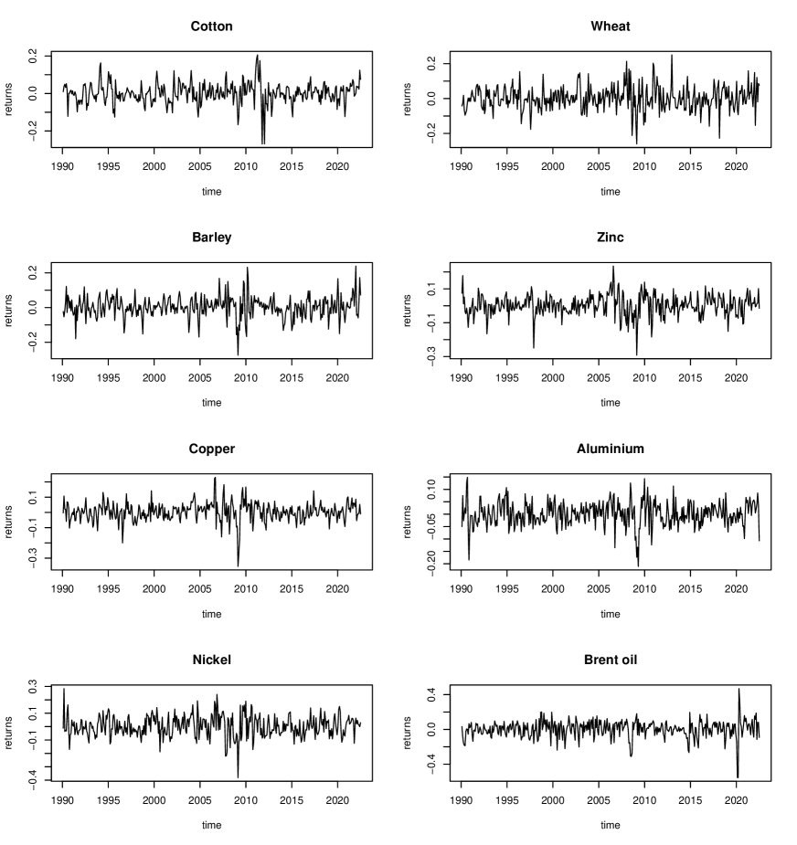
Figure 9: Log-returns

References

\NAT@swatrue
Alekseev (1996)
Alekseev, V. (1996).
Asymptotic properties of higher-order periodograms.
Theory of Probability & Its
Applications, 40(3), 409–419.
\NAT@swatrue
Andrews et al. (2009)
Andrews, B., Calder, M., and Davis, R. A. (2009).
Maximum likelihood estimation for -stable
autoregressive processes.
The Annals of Statistics, 37(4), 1946–1982.
\NAT@swatrue
Andrews et al. (2006)
Andrews, B., Davis, R. A., and Breidt, F. J. (2006).
Maximum likelihood estimation for all-pass time series
models.
Journal of Multivariate Analysis, 97(7), 1638–1659.
\NAT@swatrue
Anh et al. (2007)
Anh, V., Leonenko, N. N., and Sakhno, L. (2007).
Minimum contrast estimation of
random processes based on information of second and third orders.
Journal of statistical planning and
inference, 137(4), 1302–1331.
\NAT@swatrue
Bartelt et al. (1984)
Bartelt, H., Lohmann, A. W., and Wirnitzer, B. (1984).
Phase and
amplitude recovery from bispectra.
Applied optics, 23(18), 3121–3129.
\NAT@swatrue
Bartlett (1950)
Bartlett, M. S. (1950).
Periodogram analysis and continuous spectra.
Biometrika, 37(1/2), 1–16.
\NAT@swatrue
Basawa et al. (1976)
Basawa, I., Feigin, P., and Heyde, C. (1976).
Asymptotic properties of maximum likelihood
estimators for stochastic processes.
Sankhyā: The Indian Journal of Statistics, Series
A, 259–270.
\NAT@swatrue
Bec et al. (2020)
Bec, F., Nielsen, H. B., and Saïdi, S. (2020).
Mixed causal–noncausal
autoregressions: Bimodality issues in estimation and unit root testing
1.
Oxford Bulletin of Economics and
Statistics, 82(6), 1413–1428.
\NAT@swatrue
Breid et al. (1991)
Breid, F. J., Davis, R. A., Lh, K.-S., and Rosenblatt, M. (1991).
Maximum likelihood estimation for noncausal
autoregressive processes.
Journal of Multivariate Analysis, 36(2), 175–198.
\NAT@swatrue
Brillinger (1974)
Brillinger, D. R. (1974).
Cross-spectral
analysis of processes with stationary increments including the stationary
g/g/ queue.
The Annals of Probability, 815–827.
\NAT@swatrue
Brillinger (1975)
Brillinger, D. R. (1975).
Time series. data analysis and theory. holt, renehart and
winston.
Inc., New York.
\NAT@swatrue
Brillinger (1985)
Brillinger, D. R. (1985).
Fourier inference: Some methods for the
analysis of array and nongaussian series data 1.
JAWRA Journal of the American Water Resources
Association, 21(5), 743–756.
\NAT@swatrue
Brillinger and Rosenblatt (1967)
Brillinger, D. R., and Rosenblatt, M. (1967).
Asymptotic theory of estimates of kth-order spectra.
Proceedings of the National Academy of Sciences of the
United States of America, 57(2), 206.
\NAT@swatrue
Brockwell and Davis (1987)
Brockwell, P. J., and Davis, R. A. (1987).
Time series: theory and
methods.
Springer-Verlag. New York.
\NAT@swatrue
Cubadda et al. (2019)
Cubadda, G., Hecq, A., and Telg, S. (2019).
Detecting co-movements in non-causal time series.
Oxford Bulletin of Economics and
Statistics, 81(3), 697–715.
\NAT@swatrue
Fries (2021)
Fries, S. (2021).
Conditional moments of noncausal
alpha-stable processes and the prediction of bubble crash odds.
Journal of Business & Economic Statistics, 1–21.
\NAT@swatrue
Fries and Zakoian (2019)
Fries, S., and Zakoian, J.-M. (2019).
Mixed causal-noncausal ar processes and the modelling of
explosive bubbles.
Econometric Theory, 35(6), 1234–1270.
\NAT@swatrue
Giancaterini and Hecq (2022)
Giancaterini, F., and Hecq, A. (2022).
Inference in mixed causal and
noncausal models with generalized student’s t-distributions.
Econometrics and Statistics.
\NAT@swatrue
Giannakis and Swami (1990)
Giannakis, G. B., and Swami, A. (1990).
On estimating noncausal nonminimum phase arma models
of non-gaussian processes.
IEEE transactions on acoustics, speech, and signal
processing, 38(3), 478–495.
\NAT@swatrue
Gourieroux and Jasiak (2018)
Gourieroux, C., and Jasiak, J. (2018).
Misspecification of noncausal order in autoregressive
processes.
Journal of Econometrics, 205(1), 226–248.
\NAT@swatrue
Gourieroux et al. (2021)
Gourieroux, C., Jasiak, J., and Tong, M. (2021).
Convolution-based filtering and
forecasting: An application to wti crude oil prices.
Journal of Forecasting, 40(7), 1230–1244.
\NAT@swatrue
Gouriéroux and Zakoïan (2017)
Gouriéroux, C., and Zakoïan, J.-M. (2017).
Local
explosion modelling by non-causal process.
Journal of the Royal Statistical Society: Series B
(Statistical Methodology), 79(3), 737–756.
\NAT@swatrue
Hamilton (2018)
Hamilton, J. D. (2018).
Why you should never use the hodrick-prescott filter.
Review of Economics and Statistics, 100(5), 831–843.
\NAT@swatrue
Hansen and Sargent (1991)
Hansen, L. P., and Sargent, T. J. (1991).
Two difficulties in interpreting vector autoregressions.
In Rational
expectations econometrics (pp. 77–120).
CRC Press.
\NAT@swatrue
Hecq et al. (2020)
Hecq, A., Issler, J. V., and Telg, S. (2020).
Mixed causal–noncausal autoregressions with exogenous
regressors.
Journal of Applied Econometrics, 35(3), 328–343.
\NAT@swatrue
Hecq et al. (2016)
Hecq, A., Lieb, L., and Telg, S. (2016).
Identification of mixed causal-noncausal models in finite
samples.
Annals of Economics and Statistics/Annales
d’Économie et de Statistique(123/124), 307–331.
\NAT@swatrue
Hecq, Lieb, and Telg (2017)
Hecq, A., Lieb, L., and Telg, S. (2017).
Simulation,
estimation and selection of mixed causal-noncausal autoregressive models: The
marx package.
Available at SSRN 3015797.
\NAT@swatrue
Hecq, Telg, and Lieb (2017)
Hecq, A., Telg, S., and Lieb, L. (2017).
Do seasonal adjustments induce noncausal dynamics in
inflation rates?
Econometrics, 5(4), 48.
\NAT@swatrue
Hecq and Voisin (2019)
Hecq, A., and Voisin, E. (2019).
Predicting bubble
bursts in oil prices during the covid-19 pandemic with mixed causal-noncausal
models.
arXiv preprint arXiv:1911.10916.
\NAT@swatrue
Hecq and Voisin (2021)
Hecq, A., and Voisin, E. (2021).
Forecasting bubbles with mixed causal-noncausal
autoregressive models.
Econometrics and Statistics, 20, 29–45.
\NAT@swatrue
Hencic and Gouriéroux (2015)
Hencic, A., and Gouriéroux, C. (2015).
Noncausal autoregressive model in application to
bitcoin/usd exchange rates.
In Econometrics of risk (pp. 17–40).
Springer.
\NAT@swatrue
Huang and Pawitan (2000)
Huang, J., and Pawitan, Y. (2000).
Quasi-likelihood estimation of non-invertible moving
average processes.
Scandinavian Journal of Statistics, 27(4), 689–702.
\NAT@swatrue
Karapanagiotidis (2014)
Karapanagiotidis, P. (2014).
Dynamic
modeling of commodity futures prices.
\NAT@swatrue
Kay and Marple (1981)
Kay, S. M., and Marple, S. L. (1981).
Spectrum
analysis—a modern perspective.
Proceedings of the IEEE, 69(11), 1380–1419.
\NAT@swatrue
Kindop (2021)
Kindop, I. (2021).
Ubiquitous multimodality in mixed causal-noncausal
processes.
\NAT@swatrue
Lanne and Luoto (2012)
Lanne, M., and Luoto, J. (2012).
Has
us inflation really become harder to forecast?
Economics Letters, 115(3), 383–386.
\NAT@swatrue
Lanne et al. (2012)
Lanne, M., Luoto, J., and Saikkonen, P. (2012).
Optimal forecasting of noncausal autoregressive time series.
International Journal of Forecasting, 28(3), 623–631.
\NAT@swatrue
Lanne and Saikkonen (2011)
Lanne, M., and Saikkonen, P. (2011).
Noncausal autoregressions for economic time series.
Journal of Time Series Econometrics, 3(3).
\NAT@swatrue
Lehr and Lii (1998)
Lehr, M. E., and Lii, K.-S. (1998).
Maximum likelihood estimates of non-gaussian arma models.
University of California Riverside.
\NAT@swatrue
Leonenko et al. (1998)
Leonenko, N. N., Sikorskii, A. Y., and Terdik, G. (1998).
On spectral and bispectral estimator of the parameter of
nongaussian data.
\NAT@swatrue
K. Lii and Rosenblatt (1982)
Lii, K., and Rosenblatt, M. (1982).
Deconvolution and estimation of transfer function phase and
coefficients for nongaussian linear processes: The annals of statistics, v.
lo.
\NAT@swatrue
K.-S. Lii and Rosenblatt (1992)
Lii, K.-S., and Rosenblatt, M. (1992).
An approximate
maximum likelihood estimation for non-gaussian non-minimum phase moving
average processes.
Journal of Multivariate Analysis, 43(2), 272–299.
\NAT@swatrue
K.-S. Lii and Rosenblatt (1996)
Lii, K.-S., and Rosenblatt, M. (1996).
Maximum likelihood estimation for nongaussian
nonminimum phase arma sequences.
Statistica Sinica, 1–22.
\NAT@swatrue
Lobato and Velasco (2022)
Lobato, I. N., and Velasco, C. (2022).
Single step estimation of arma roots for
nonfundamental nonstationary fractional models.
The Econometrics Journal, 25(2), 455–476.
\NAT@swatrue
Lof (2013)
Lof, M. (2013).
Noncausality and asset
pricing.
Studies in Nonlinear Dynamics and
Econometrics, 17(2), 211–220.
\NAT@swatrue
Lof and Nyberg (2017)
Lof, M., and Nyberg, H. (2017).
Noncausality and the commodity currency hypothesis.
Energy Economics, 65, 424–433.
\NAT@swatrue
Nikias and Chiang (1987)
Nikias, C., and Chiang, H.-H. (1987).
Non-casual autoregressive bispectrum estimation and
deconvolution.
In Icassp’87. ieee international conference on
acoustics, speech, and signal processing (Vol. 12, pp. 1557–1560).
\NAT@swatrue
Rao and Gabr (1989)
Rao, T. S., and Gabr, M. (1989).
The estimation of the bispectral
density function and the detection of periodicities in a signal.
In Multivariate
statistics and probability (pp. 484–504).
Elsevier.
\NAT@swatrue
Rao and Gabr (2012)
Rao, T. S., and Gabr, M. (2012).
An introduction to bispectral analysis and bilinear time series
models (Vol. 24).
Springer Science & Business Media.
\NAT@swatrue
Rosenblatt (1965)
Rosenblatt, M. (1965).
Stationary sequences
and random fields.
Springer Science & Business Media.
\NAT@swatrue
Rosenblatt (1980)
Rosenblatt, M. (1980).
Linear processes and
bispectra.
Journal of Applied Probability, 17(1), 265–270.
\NAT@swatrue
Rosenblatt and Van Ness (1965)
Rosenblatt, M., and Van Ness, J. W. (1965).
Estimation of the
bispectrum.
The Annals of Mathematical Statistics, 1120–1136.
\NAT@swatrue
Schuster (1898)
Schuster, A. (1898).
On the
investigation of hidden periodicities with application to a supposed 26 day
period of meteorological phenomena.
Terrestrial Magnetism, 3(1), 13–41.
\NAT@swatrue
Terdik (1999)
Terdik, G. (1999).
Bilinear stochastic
models and related problems of nonlinear time series analysis: a frequency
domain approach (Vol. 142).
Springer Science & Business Media.
\NAT@swatrue
Tugnait (1986)
Tugnait, J. K. (1986).
Identification of non-minimum phase linear stochastic
systems.
Automatica, 22(4), 457–464.
\NAT@swatrue
Velasco and Lobato (2018)
Velasco, C., and Lobato, I. N. (2018).
Frequency domain minimum distance
inference for possibly noninvertible and noncausal arma models.
The Annals of Statistics, 46(2), 555–579.
\NAT@swatrue
Whittle (1953)
Whittle, P. (1953).
Estimation and information in stationary time series.
Arkiv för matematik, 2(5), 423–434.