Non-monotonic behavior of timescales of passage in heterogeneous media: Dependence on the nature of barriers

Abstract

Usually time of passage across a region may be expected to increase with the number of barriers along the path. Can this intuition fail depending on the special nature of the barrier? We study experimentally the transport of a robotic bug which navigates through a spatially patterned array of obstacles. Depending on the nature of the obstacles we call them either entropic or energetic barriers. For energetic barriers we find that the timescales of first passage vary non-monotonically with the number of barriers, while for entropic barriers first passage times increase monotonically. We perform an exact analytic calculation to derive closed form solutions for the mean first passage time for different theoretical models of diffusion. Our analytic results capture this counter-intuitive non-monotonic behaviour for energetic barriers. We also show non-monotonic effective diffusivity in the case of energetic barriers. Finally, using numerical simulations, we show this non-monotonic behaviour for energetic barriers continues to hold true for super-diffusive transport. These results may be relevant for timescales of intra-cellular biological processes.

Introduction

Random walks arise in multiple physical, geological, biological and ecological contexts as simple models of stochastic transport [1, 2, 3, 4]. In particular, random walks have been used to model stochastic transport inside cells. Some well-known examples are motor proteins carrying cargo on networks of microtubules [5, 6, 7], RNA polymerase moving on DNA during transcription and backtracking [8, 9, 10], loop extrusion of DNA through motion of cohesin and condensin proteins [11, 12, 13, 14, 15, 16, 17], and motion of transcription factors on DNA as it searches for binding sites [18, 19].

For physical and biological systems, often the environment in which diffusion happens is complex, characterised by heterogeneous media with frequent obstacles. The motion of bacteria in soil, a 3D porous medium, is relevant in agriculture [20, 21] and the problem has been studied experimentally [22]. Intracellular transport processes are hindered by the presence macromolecular crowders [23, 24]. Apart from cytoplasmic crowding, barriers may appear in the form of steric hindrance, for example, by nucleosomes to the motion of RNA polymerase during transcription [25, 26] and to cohesin proteins during chromatin looping [27]. During diffusion of morphogens in early Drosophila embryos, membrane furrows between neighbouring nucleocytoplasmic compartments cause heterogeneous diffusion, acting as obstacles to diffusive transport and gradient formation [28, 29]. Obstacles can thus affect timescales of critical biological processes – namely transcription completion and DNA repair times, chromatin looping times, morphogen gradient formation times in embryogenesis, etc.

In the context of such random motion through heterogeneous media, a relevant question is how effective transport coefficients arise through the interaction of the walker with the environment [30]. Another interesting question is completion times of transport which may lead to important biological events, referred to in the literature as first passage times [2, 7, 31, 32, 33]. For example, search and capture of kinetochores by mobile microtubules [34, 35], binding of proteins (such as TATA binding protein, RNA polymerase, cohesin) to preferred locations of DNA [36, 27], threshold crossing of protein numbers triggering cell lysis [37, 38, 39] and cell division [40], all constitute examples where estimating first passage times are crucial to understanding timescales of biological processes.

The role of disorder and barrier in transport may sometimes be counterintuitive. Usual expectations would be that obstacles slow down transport, suppress effective diffusivity, enhance path lengths, and increase mean and fluctuation of first passage times. Contrary to this, experimental studies of particle transport in crowded spaces have shown unexpected non-monotonic behavior. For example, a study of bacterial transport through a system of microscopic scatterers showed non-monotonic behavior of effective propagation distance and effective propagation speed as a function of the obstacle density [41]. Instead of obstacles increasing times spent within a confinement, they may shorten it by decreasing the total accessible surface area [42]. In a study of a self propelled camphor boat moving through passive movable crowders in 2D, fluctuations of first passage time were shown to be non-monotonic as a function of the obstacle density, although the mean was still monotonic in nature [43].

Our current study explores passage times in heterogeneous environments and its counterintuitive dependence on the nature of the barriers. This is partially motivated by a puzzle presented by an experimental study of diffusion of cohesin protein on DNA in the context of chromatin loop extrusion [27]. Nucleosomes act as barriers to purely diffusive motion of cohesin across the DNA backbone. Measurement of permeability index for cohesin on DNA through these barriers indicated reduction of diffusivity. Intuitively as number of barriers increase, looping time should rise, but estimates at high nucleosome density gave biophysically impossible loop formation times. A resolution was suggested through a simulation study which showed that with increase in the number of barriers there is a non monotonic behavior of loop formation times [11]. Thus, quite counter-intuitively, the looping times can be of the order of relevant biophysical timescales even when number of nucleosomes are large.

Several questions present themselves in the light of the above two studies. Firstly, is it generically true that timescales of passage show non-monotonic behavior with the number of barriers? Would this result still hold for macroscopic scales far greater than these nanoscopic lengthscales of DNA and nucleosomes? Further, would this non-monotonic behavior hold true for superdiffusive transport? We address each of these questions systematically using a combination of experiments, exact analytic calculations and kinetic simulations. We show that the non-monotonic behavior of passage times generically persists at macroscopic scales, but crucially depends on the nature of the barriers.

One may broadly define two classes of barriers – entropic vs energetic, with distinct transport properties [44, 45]. While energetic barriers involve activation energy in passing from one potential minima to another, entropic barriers arise due to configurational entropy differences associated with structural heterogeneity in a system [46, 47, 22]. In models of glass transition, the nature of barriers, whether energetic or entropic, crucially determine the nature of timescale variation [48]. In our experiments, we implement the two distinct types of barriers through two different design principles. We show that while the non monotonicity in timescales of passage is observed for energetic barriers, it is not observed in the case of entropic barriers.

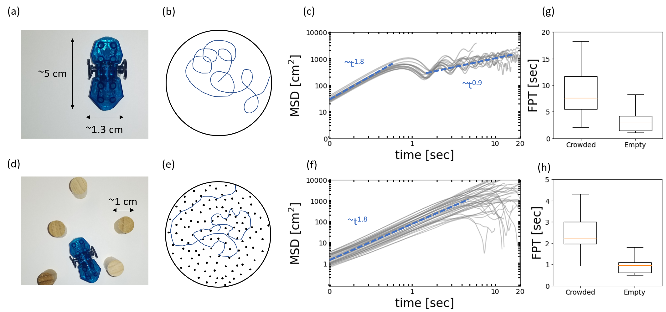
Figure 1: (a) A robotic bug (HEXBUG) is shown with scale bars. (b) Sample trajectory of a bug in empty circular space of diameter 117$cm$. (c) Mean square displacement of the bug as a function of time in the bulk empty space displaying a superdiffusive behavior (dotted line slope $\sim$ 1.8) for short times which becomes more diffusive with a fitted slope $\sim$ 1. (d) Robotic bug alongside wooden pegs with respective scalebar. (e) Sample trajectory of bug in crowded space filled at a packing fraction of 6 $\%$. (f) Mean square displacement of bug through the bulk crowded area shows superdiffusive behavior with a fitted slope $\sim$ 1.8. (g) The mean first passage time of robotic bug in the empty circular region (panel b) is recorded to be 3.95 secs and for the crowded region (panel e) is recorded to be 8.63 secs. (h)The mean first passage time of robotic bug in a crowded rectangular region of dimensions 76 $\times$ 27 cm is recorded to be 2.5 times higher than equivalent empty region.

Results

Experiments reveal the crucial role of the nature of barriers in controlling first passage

We design a simple experiment to probe the role of barriers in regulating first passage times. The random walker (RW) is a self-propelled robotic bug of dimensions $1.3cm\times 5cm$ (see Fig 1a). For most of our experiments the bug moves through a rectangular region of dimensions $180cm\times 76cm$ having an array of obstacles (see Methods for more details). We first characterize the motion of the random walker in a circular region of diameter 117 $cm$, and show a sample trajectory in Fig. 1b. The mean square displacement of the bug reveals a superdiffusive behavior ($\langle x^{2}(t)\rangle\sim t^{1.8}$) at short time scales, crossing over to a diffusive behavior at longer time scales ($\langle x^{2}(t)\rangle\sim t^{0.9}$), as shown in Fig. 1c.

Designing Entropic barriers

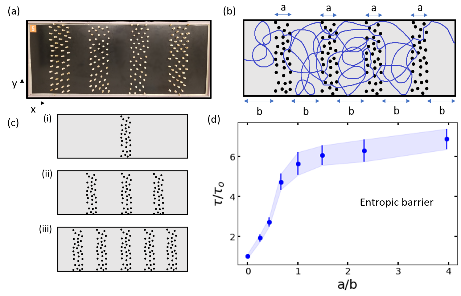
Figure 2: (a) Top view of the implemented 2D patterned geometry of alternate barrier and empty regions for entropic barriers. (b) Sample trajectory of bug this region. We record the first passage time as the time taken for the bug to cross the patterned area from the left boundary to the right, for the first time. Presence of the barriers slows down the bug which can move around or bounce from the wooden pegs in the barrier region to change its direction. Barrier regions have a fixed width $a$, width of the empty region is depicted by variable $b$ (c) Schematic of arrangement of barriers for successive setups gives an idea of the experimental protocol. We systematically increase the number of barriers to find the first passage time for each setup. (d) Normalized mean first passage time is plotted as a function of $a/b$. The MFPT increases monotonically with $a/b$, and saturates for high number of barriers.

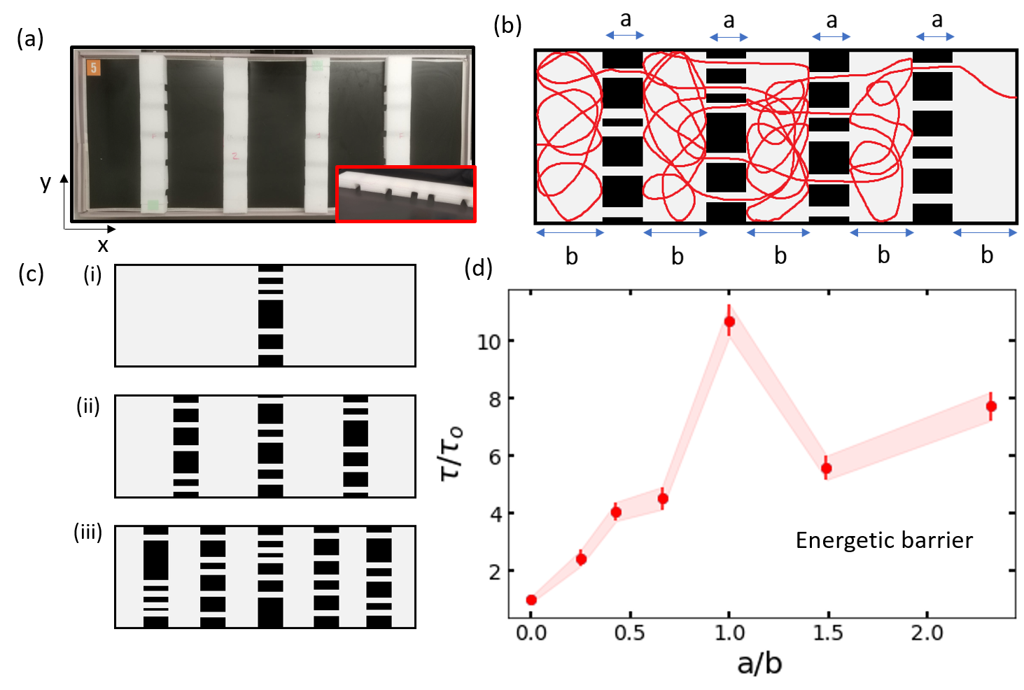
Figure 3: (a)Top view of implemented patterned geometry with alternate energetic barrier and empty regions. The barriers have tunnels cut at 5 random positions along its length. Inset depicts a side view of the styrofoam barrier. The individual tunnels are of size $3$cm. (b) Sample trajectory of bug through an arrangement of alternate empty (width $b$) and impenetrable (tunnel) barrier (of width $a$) regions. Trajectories show random motion of the bug in the empty regions, and an instantaneous motion through the tunnels whenever it finds them. Time taken to travel from one end of boundary along its width $180$cm is defined as the first passage time. (c)Schematic of arrangement of impenetrable barriers for successive setups. We systematically increase the number of barrier regions to find the first passage time for each setup. (d) Normalized mean first passage time is plotted as a function of $a/b$. Each data point is an average over 100 trials. We observe a non-monotonic behavior of the mean first passage time with increasing $a/b$.

One way to introduce barriers to the motion of the RW is to construct regions where the free motion of the RW is impeded. To this end, we used wooden pegs of diameter $1cm$ arranged randomly at a packing fraction of $6\%$ to constitute a crowded barrier region. An image of our self-propelled bug alongside the pegs is shown in Fig. 1d. In order to verify that these crowded regions indeed serve as barriers, we characterised the motion of the RW in a circle of diameter $117cm$, filled with the wooden pegs. A sample trajectory in this region is shown in Fig. 1e. Again, as in the case of the motion in the absence of any barriers, the mean square displacement showed a superdiffusive behavior with a similar exponent, $\langle x^{2}(t)\rangle\sim t^{1.8}$ (Fig. 1f). Curiously, there was no clear signature of a transition to diffusive transport in this case, as opposed to the motion in free space. However, the transport is slowed down as compared to the free case due to repeated collision with the pegs. The mean time to reach the boundary of the crowded circular region starting from the center was $8.63\pm 0.49sec$, as compared to a mean time of $3.95\pm 0.39sec$ in the absence of barriers (Fig. 1g).

Having established that a region filled with wooden pegs do indeed slow down the motion of the RW, we constructed rectangular barrier regions of width $a=27cm$ filled with wooden pegs at the same packing fraction of $6\%$. Note that for such barriers the mean time of passage is about $2.5$ times larger than that for empty regions of equivalent width (Fig. 1h). Sample trajectories and mean square displacement in these empty and crowded rectangular regions are shown in Suppl Fig. 3a and 3c. The superdiffusive motion persists in this geometry (Suppl Fig. 3b and 3d). We then proceeded to investigate the first passage properties of the system in the presence of multiple such barrier regions, shown in Fig. 2a. A sample trajectory in such a setup with four barriers is shown in Fig. 2b. We call this type of barriers as entropic, as the time delay in navigation through them is due to exploration of multiple positional configurations resulting from collisions with the pegs. The number $n$ of barriers is varied between 1-7, and some configurations are schematically shown in Fig. 2c(i)-(iii). Note that as the total length of the system was fixed ($L=180cm$), increasing $n$ automatically implies that the spacing $b$ between the barriers reduce. For a fixed $n$, we are interested in the stochastic first passage of the bug starting from $x=0$ and reaching $x=L$ for the first time. We find the times $T$ of such passage in 100 different experimental trials and evaluated the mean first passage time (MFPT), $\tau=\langle T\rangle$.

The behavior of the MFPT is shown in Fig. 2d as a function of the dimensionless ratio of the two widths of the barrier and free regions, namely $a/b$. Initially, when the number of barriers is very low, the MFPT increases rapidly with increasing barrier number. However, the increase saturates at high barrier numbers as the system essentially becomes covered with the barrier regions. As the number of barriers, $n$, increases, the width of the free region decreases, and hence $a/b$ increases. The behavior of $\tau$ versus $a/b$ is monotonic as expected – more the number of barriers, slower the navigation.

Designing Energetic barriers

We now ask whether one may design another kind of barriers which may lead to a distinct behavior of first passage times. We used styrofoam blocks as barriers with five tunnel-like passages of width $3cm$ cut through them at random positions along their length (Fig.3a). A representative trajectory of passage from $x=0$ to $x=L$ is shown in Fig. 3b. Note that as the bug encounters the barrier, it most often gets reflected back into the free regions since the probability that it finds one of the five open tunnels at the right orientation is low. However,in contrast to the entropic barriers, once the bug enters into any of these tunnels, it passes through in a straight line, in a meagre time $\lesssim 1s$. Thus these barriers mimic the physics of energetic barriers, where the major delay comes from repeated attempts and failure to find a tunnel to go through, equivalent to moving uphill from a valley to a hilltop along an energy landscape. As in the case of entropic barriers, each barrier region of width $a=20cm$ was positioned alternately with empty regions of width $b$, and we varied the the number $n$ of the barriers (Fig. 3c). As before, when $n$ increases, $b$ decreases and $a/b$ rises.

We plot the behavior of the mean first passage time $\tau$ for this array of energetic barrier arrangement as a function of the $a/b$ ratio in Fig. 3d. For low number of barriers, the MFPT increases with increasing barrier number. However, as the $a/b$ ratio approaches the value $\sim 1$, the MFPT exhibits a local maximum. Increasing the number of barriers beyond this results in a decline of MFPT. Note that there is a slight increase of the MFPT again at $a/b\simeq 2.5$, however this increase is an artefact of the finite size of our experimental setup (see Methods for more details). This striking behavior of a non-monotonic variation of MFPTs with increasing barrier numbers is in sharp contrast to the monotonic increase followed by saturation seen for entropic barriers. This suggests that the nature of the barriers play a crucial role in controlling the statistics of first passage times.

Exact analytical results confirm the differential role of energetic and entropic barriers

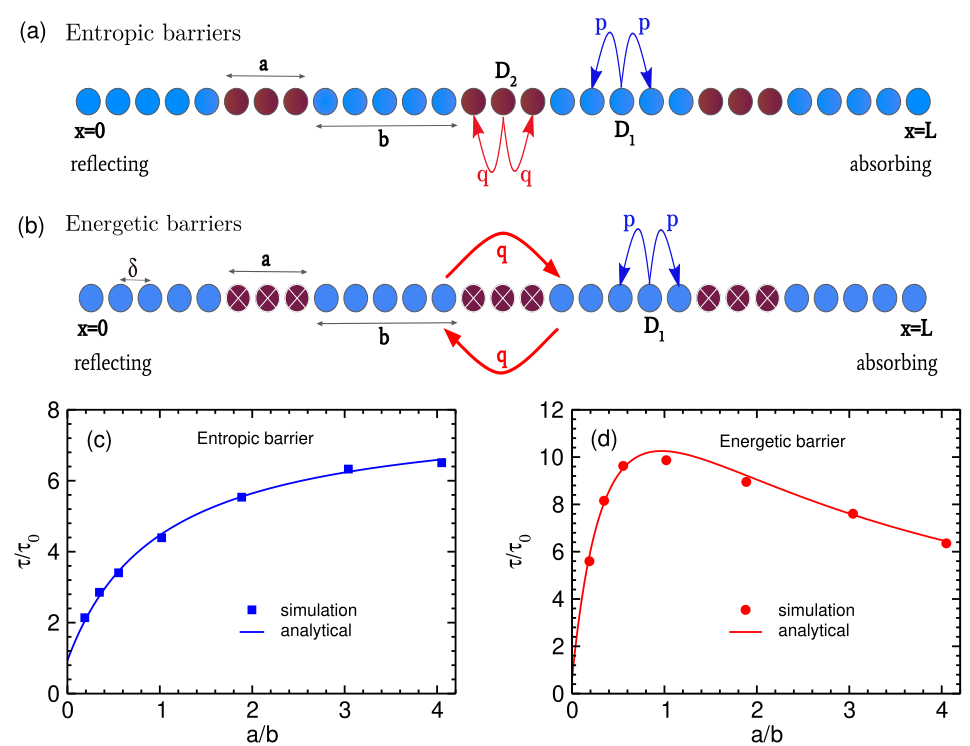
Figure 4: (a) Schematic of the system used in simulation in presence of entropic barriers. $a$ and $b$ denotes the width of the barrier region and the free region respectively.The hopping rates in the free and barrier region are given by $p$ and $q$ respectively which corresponds to diffusion constants $D_{1}$ and $D_{2}$. (b) Schematic of the system in presence of energetic barriers. The hopping rate across the barrier is given by $q$. When successful, the RW hops the barrier width $a$. $\delta$ denotes the lattice constant. (c-d) Scaled MFPT vs ratio of barrier width and average gap in case of entropic barriers and energetic barriers respectively for a diffusive particle. The data is shown for the ratio $D_{1}/D_{2}=8$ for entropic barriers, and for $D_{1}/(2av_{q})=20/3$ for energetic barriers. for for we The solid lines are obtained from analytical calculations (Eq. 39 for entropic barriers, and Eq. 9 for energetic barriers) while the points are the simulation results.

Motivated by the interesting experimental results above, we turn to a theoretical formulation of a simplified random walk model of transport in the presence barriers to understand this phenomenon. In order to simplify the analysis, we study a diffusion problem in one dimension exactly, in the presence of both entropic and energetic barriers.

In the absence of any barriers, the motion in the bulk is simple unbiased diffusion with diffusion constant $D_{1}$. Motivated by the experimental conditions, a random walker starts at $x=0$ which is modeled as a reflecting boundary. The FPT, again in analogy to experiments, is defined as the time the particle reaches $x=L$ (right boundary) for the first time. We impose absorbing boundary conditions at $x=L$. The Mean First Passage Time (MFPT) in this case is simply $\tau_{0}=L^{2}/2D_{1}$ [1].

Entropic Barriers

We first consider the case for entropic barriers, implemented as slow regions where the particle still performs diffusive motion, with a diffusion coefficient $D_{2}$ smaller than in the bulk, that is, $D_{2}<D_{1}$. The slow regions have width $a$, and the fast regions have width $b$, and the whole length $L$ is covered by an array of $n$ barriers, such that $L=b+n(a+b)$. The setup for this configuration is shown in Fig. 4(a).

The particle starts at $x=0$ at time $t=0$. The reflecting and absorbing boundary conditions at the left and right boundaries can be expressed as,

$$\partial_{x}\langle T\rangle_{x=0}=0~{}~{}~{}\mathrm{and}~{}~{}~{}\langle T\rangle_{x=L}=0$$ (1)

For a system with $n$ regularly spaced barriers, there are thus $n+1$ empty regions, and the MFPT in all these regions obey [1]

$$D_{1}\frac{\partial^{2}\langle T_{2i-1}\rangle}{\partial x^{2}} = -1~{}~{}~{}~{}~{}~{}i\in(1,n+1)$$ (2)

$$D_{2}\frac{\partial^{2}\langle T_{2i}\rangle}{\partial x^{2}} = -1~{}~{}~{}~{}~{}~{}i\in(1,n)$$ (3)

where the subscript of $T$ labels all the $2n+1$ alternating empty and barrier regions.

In order to solve these equations, we need the boundary conditions at the barrier interfaces. Let the boundary points of $i^{th}$ barrier be denoted by $x_{2i-1}$ and $x_{2i}$ which satisfy,

$$x_{2i-1} = b+(i-1)(a+b)~{}~{}~{}~{}~{}i\in(1,n)$$

$$x_{2i} = i(a+b)~{}~{}~{}~{}~{}~{}~{}~{}~{}~{}~{}~{}~{}~{}~{}~{}~{}~{}i\in(1,n)$$ (4)

At these barrier interfaces, the mean times as well as the corresponding “fluxes” must be continuous. This leads to the following conditions on the times at the barrier boundaries (see Supplementary Information Sec. I and Suppl. Fig. 1)

$$\langle T_{2i-1}\rangle_{x_{2i-1}} = \langle T_{2i}\rangle_{x_{2i-1}}~{}~{}~{}~{}~{}~{}~{}~{}~{}~{}i\in(1,n)$$

$$D_{1}\partial_{x}\langle T_{2i-1}\rangle_{x_{2i-1}} = D_{2}\partial_{x}\langle T_{2i}\rangle_{x_{2i-1}}~{}~{}~{}i\in(1,n)$$

$$\langle T_{2i}\rangle_{x_{2i}} = \langle T_{2i+1}\rangle_{x_{2i}}~{}~{}~{}~{}~{}~{}~{}~{}~{}~{}i\in(1,n)$$

$$D_{2}\partial_{x}\langle T_{2i}\rangle_{x_{2i}} = D_{1}\partial_{x}\langle T_{2i+1}\rangle_{x_{2i}}~{}~{}~{}i\in(1,n)$$ (5)

The equations  15 and  16 can be solved exactly subject to the boundary conditions (Eq.  1) and the matching conditions at the barrier interfaces, Eq.  5 (see Supplementary Information Sec. I for detailed calculation). This gives the scaled MFPT of the particle to reach $x=L$ starting from $x=0$ in presence of $n$ barriers of width $a$ as,

$$\frac{\tau}{\tau_{0}}=\frac{\langle T_{1}\rangle_{x=0}}{\tau_{0}}=1+\frac{(s-1)(r-a/L)}{1+r}$$ (6)

where $r=a/b$ denotes the ratio of the barrier size to the size of the empty regions, and $s=D_{1}/D_{2}>1$ denotes the ratio between diffusion constants in two regions.

As can be seen from the form of the expression, the MFPT increases monotonically with the ratio $r=a/b$. It saturates for large $r$ to the limiting value $\tau=s\tau_{0}$. This behavior is shown in Fig. 4(c) where the analytical result of Eq. 39 is compared with simulation results. Consistent with the experimental findings, entropic barriers – modeled through regions of slow diffusion – do not lead to any non-monotonic behavior of first passage times.

Energetic Barriers

Having established that entropic barriers do not lead to any non-monotonicity in first passage times, we now turn to the case of energetic barriers. Energetic barriers are modeled as blocked regions of width $a$ separated by empty regions of width $b$ where free diffusion may happen. The diffusion constant in continuum is $D_{1}$ for the empty regions. For the analogous discrete model (with lattice spacing $\delta$), on which simulations are performed, the unbiased forward and backward hopping rates are $p$. For hopping across a barrier from one empty region to another, the rate is $q~{}(\ll p)$. The usual discrete to continuum correspondence implies $D_{1}=p\delta^{2}$ and a barrier hopping velocity $v_{q}=q\delta$, in the limit $\delta\rightarrow 0$ and $p,q\rightarrow\infty$. If there are $n$ such barriers then the total length $L=b+n(a+b)$. A schematic for this configuration on lattice is shown in Fig. 4(b).

We proceed to solve the problem in continuous space. For $n$ barriers, and $n+1$ free regions, the MFPT in the $i^{th}$ free region ($2i-1^{th}$ region overall) follows [1]

$$D_{1}\partial_{x}^{2}\langle T_{2i-1}\rangle=-1,$$ (7)

with $i\in\{1,n+1\}$. The boundary conditions at the barrier interfaces are non-trivial (see Supplementary Information Sec. II and Suppl. Fig. 2 for details)

$$\langle T_{2i-1}\rangle_{x_{2i-1}} = \langle T_{2i+1}\rangle_{x_{2i}}-\frac{D_{1}}{v_{q}}\partial_{x}\langle T_{2i-1}\rangle_{x_{2i-1}}$$

$$\partial_{x}\langle T_{2i-1}\rangle_{x_{2i-1}} = \partial_{x}\langle T_{2i+1}\rangle_{x_{2i}}.$$ (8)

We solve Eq. 7 subject to the reflecting and absorbing boundary conditions at $x=0$ and $x=L$ (Eq. 1), and the matching conditions at the barrier interfaces, Eq. 8. These lead to the scaled MFPT of a random walker starting from $x=0$ to reach $x=L$ in the presence of $n$ energetic barriers as,

$$\frac{\tau}{\tau_{0}}=\frac{\left(1+\frac{a}{L}\right)^{2}+\left(r-\frac{a}{L}\right)\left(1+\frac{L}{a}\right)\frac{D_{1}}{Lv_{q}}}{(1+r)^{2}}$$ (9)

where again $r=a/b$.

Note that unlike in the case for entropic barriers, the functional dependence of the MFPT on $r=a/b$ (in Eq. 9) implies a maximum in the MFPT as a function of $r$. This can be seen in Fig.  4(d) where the analytical result of Eq. 9 is compared with simulation results. Quite remarkably, our simple calculation based on diffusive transport accurately captures the main qualitative trend of the experimental data of Fig.  3d of a maximum in the MFPT.

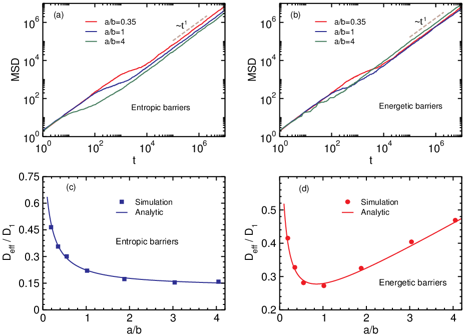
Figure 5: (a-b) Mean Squared Displacement (MSD) vs time is plotted with solid lines for diffusive particle in presence of entropic barriers and energetic barriers respectively. The different colours denote different ratio of barrier width and average gap ($a/b$) and the dashed line is for the guidance of the eye. (c-d) Effective diffusion constant ($D_{\mathrm{eff}}$) is shown with variation of $a/b$ in case of entropic barriers and energetic barriers respectively. The points depict the simulation results while the solid lines denote the analytical result (Eq. 11 for entropic barriers, and Eq. 12 for energetic barriers).

Curiously, both the experimental and theoretical curves suggest that the location of the maxima occurs when the width of the barrier is comparable to the width of the empty regions, $a\sim b$. The location of the maxima can be calculated from the expression of the MFPT, Eq. 9, and yields, in the $L\rightarrow\infty$ limit,

$$r^{*}=1-\frac{2av_{q}}{D_{1}}.$$ (10)

By definition, $r\geq 0$, which implies $2av_{q}/D_{1}\leq 1$. Moreover, if the hopping rate across a barrier is much lower than the bulk hopping rate, $q\ll p$, then $2av_{q}/D_{1}\ll 1$, implying that $r^{*}\simeq 1$.

Do signatures of non-trivial first passage persist in effective diffusivity?

We now ask whether this conflicting behavior for the MFPT in the presence of entropic and energetic barriers has any signature on the more common transport properties of the system. Using kinetic simulations, we characterize the Mean Square Displacement (MSD) of the random walker as a function of elapsed time in an infinite lattice in the presence of barriers. Note that, while the first passage property is history-dependent, the MSD is not.

For entropic barriers, the MSD is shown for three different $a/b$ ratios in Fig.  5(a). The RW initially explores the empty region in which it starts before it encounters the first barrier. This excursion is purely diffusive, with the bulk diffusion coefficient $D_{1}$, as is expected. At the timescale when it first encounters a barrier, the motion becomes subdiffusive as the barrier hinders the bulk diffusive behavior. Over long timescales ($t>10^{5}$), the motion becomes diffusive again, however with an effective diffusion coefficient $D_{\mathrm{eff}}~{}i.e.~{}\langle x^{2}(t)\rangle=2D_{\mathrm{eff}}t$. The value of $D_{\mathrm{eff}}$ is lower than the bulk value $D_{1}$.

As $a/b$ increases, and $b$ decreases, with increasing $n$, the transition from early diffusive to a subdiffusive regime happens faster – for $a/b=0.35,1,4$, the crossover times are $t\sim 10^{3},10^{2},5$ respectively. Moreover, with increasing $a/b$ ratio the curves in Fig. 5a at long times monotonically shift downwards. This in turn implies a monotonic decrease of $D_{\mathrm{eff}}$ as shown in Fig. 5c. An analytical formula for $D_{\mathrm{eff}}$ exists in the literature [49, 50] and can also be obtained by taking the $L\rightarrow\infty$ limit in Eq. 39 and expressing the MFPT as $\tau=L^{2}/2D_{\mathrm{eff}}$, yielding

$$D_{\mathrm{eff}}=D_{1}\left(\frac{1+r}{1+rs}\right).$$ (11)

The comparison on this analytical expression with the simulation is shown in Fig. 5c. This monotonic behavior is consistent with the monotonic increase on the MFPT for entropic barriers in a finite domain.

Next we turn to a similar characterization for the energetic barriers. The MSD of the RW on an infinite lattice, as above, is again shown for three different $a/b$ ratios in Fig. 5b. Again, for all these case, there is an initial diffusive regime with a diffusivity $D_{1}$ of the empty regions. That crosses over to a subdiffusive regime when the RW starts to feel the effect of the barriers. As expected, this transition happens earlier for the highest number of barriers ($a/b=4$), and later with decreasing $a/b$ ratios. In the long time limit, for all three $a/b$ ratios shown, the motions are again diffusive, with $\langle x^{2}\rangle=2D_{\mathrm{eff}}t$. However, quite strikingly in Fig. 5d, the MSD of the intermediate barrier number (with $a/b=1$) lies below both the cases with lower and higher barrier numbers. As a result, as shown in Fig. 5d, $D_{\mathrm{eff}}$ shows a non-monotonic behavior with increasing barrier number (or increasing $a/b$). Again, we can obtain an analytical expression for the $D_{\mathrm{eff}}$ by taking the $L\rightarrow\infty$ limit in Eq. 9 and expressing the MFPT as $\tau=L^{2}/2D_{\mathrm{eff}}$, yielding

$$D_{\mathrm{eff}}=D_{1}\left(\frac{(1+r)^{2}}{1+\frac{rD_{1}}{av_{q}}}\right).$$ (12)

which matches the simulation results exactly, as shown in Fig. 5d. Thus the signature of the non-monotonic dependence of the MFPT has its counterpart in the transport properties as well.

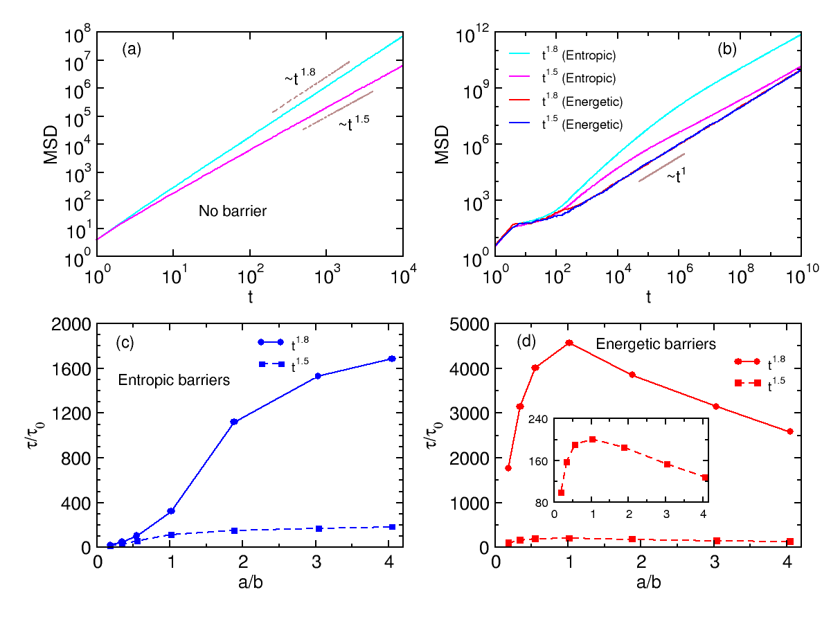
Figure 6: The figure depicts the motion of a superdiffusive particle in presence of barriers. Panel (a) shows the variation of MSD of the particle in absence of barriers while panel (b) shows the same in presence of barriers. Panels (c) and (d) denote the scaled MFPT vs $a/b$ for entropic and energetic barriers respectively. A zoomed in view of the dashed curve is shown in inset (panel (d)) to depict the non-monotonic behavior.

Is unbiased diffusion a special case? Investigating the first passage properties for superdiffusive motions

In this section we investigate whether the non-trivial dependence of the barrier number on the first passage properties for entropic and energetic barriers is quite generic, and can be extended to systems with anomalous diffusion. This enquiry is motivated by the experimental observations where the robotic bug performs superdiffusive motion over short timescales. Here we investigate the role of barriers in systems where the bulk behavior is superdiffusive.

To model superdiffusive transport in a simple one-dimensional random walk system, we use the Elephant Random Walk (ERW) model [51] that implements a non-markovian random walk with a full history-dependent memory with which it decides subsequent steps (see Methods for details). At any time, there is a probability $w$ with which it chooses its next step based on its history. It has been shown that the MSD in this case is superdiffusive: $\langle x^{2}_{t}\rangle\sim t^{4w-2}$ for $w>3/4$ [51]. We simulated the ERW for two values of $w=0.875$ and $0.95$ for which the corresponding MSD exponents are $\alpha=4w-2=1.5$ and $1.8$ respectively (see Fig. 6a). In the presence of barriers - both entropic and energetic - the MSD changes from an initial superdiffusive motion to a transient subdiffusive regime as it encounters the barriers. At longer times, the motion becomes diffusive, erasing the memory of the intrinsic superdiffusive motion in the barrier-free regions. This is shown for energetic barriers for the two superdiffusive walks in Fig. 6b. For entropic barriers, we observe the transition from an initial superdiffusive to the transient subdiffusive regime, and an approach to the limiting diffusive behavior.

On increasing the barrier numbers, the MFPT increases monotonically with the $a/b$ ratio for the case of entropic barriers, similar to the case of unbiased diffusion and our experiments. This is shown for both values of the superdiffusive exponent $\alpha$ in Fig. 6c. In contrast, for the case of energetic barriers, the MFPT again exhibits a non-monotonic behavior, similar to the case of ordinary diffusion and our experiments. The maximum of the MFPT occurs around $a/b\sim 1$, when the width of the barrier becomes equal to the length of the free regions. The differential impact of energetic and entropic barriers on first passage holds generically for different classes of RWs, and is thus very robust.

Discussion

We show that barriers may play an extremely non-trivial role in regulating first passage properties of systems. When barriers slow down transport, but allow lot of internal positional locations to be explored, we call them entropic barriers. In such cases, timescales of first passage across an array of barriers rise monotonically, as intuition would expect. Moreover the ratios of MFPT in the presence and absence of barriers saturate to a value greater than one ($s=D_{1}/D_{2}>1$), which depends on the ratio of diffusion constants in the two regions.

On the other hand, when obstacles present a barrier that allows only rare entries (but near-instantaneous transport on successful entry) into the barrier regions, we call them energetic barriers. In such cases, we show, using a combination of experiments and theory, that the timescales of first passage has a maximum when the length of the free regions matches with the width of the barrier. This is also reflected in the behavior of the effective diffusivity, which has a corresponding minimum with increasing barrier density. This is in stark contrast to naive expectations that increasing barrier density should always result in slower times of passage.

We perform an exact analytical calculation for the mean first passage times for both entropic and energetic barriers. For entropic barriers, at the barrier interfaces, the continuity of the probability and the currents (Eq. 5) allows us to derive a closed form expression for the MFPT which shows a monotonic increase with barrier numbers. For energetic barriers, the excluded barrier regions leads to a discontinuity in the mean times at the two barrier interfaces (Eq. 8), which allows to derive a closed form solution which exhibits a non-monotonic behavior with barrier numbers.

We also show that this curious behavior in the case of energetic barriers is not limited to pure diffusive transport alone, but also extends to situations where the transport is characterised by superdiffusion. Inside cells, superdiffusion has been observed for endogenous intracellular particles in crowded environments [52]. RNA polymerases and other motor proteins are also known to exhibit biased diffusion [53, 54]. The loop extrusion protein condensin is also known to exhibit superdiffusive motion on DNA backbones [14] and faces various protein obstacles which slows down loop extrusion [55]. Thus barriers may play an important role in regulating times of passage for superdiffusive transport inside cells and this can be investigated through further experimental and theoretical studies.

Regulation of first passage times are of critical importance in a variety of physical and biological systems. Our work highlights how differences in barrier design principles can crucially control times of passage in heterogeneous media. We provide a generic experimental design principle which allows us to study these two cases - one in which there is a accessible but slow region of transport through the introduction of physical obstacles, and another in which we engineer tunnels which allow only rare barrier crossing events. These designs can serve as a template for future experimental studies to investigate the relative role of these two kinds of barriers in regulating effective transport properties.

Methods

Experimental setup

A self propelled robotic bug (HEXBUG micro ant, $5cm\times 1.3cm$) (Figure 1a) powered by battery is used as a self propelled random walker. We characterized the motion of our random walker (RW) in different setups. First we consider a relatively large circular confinement of diameter $117cm$ (See Figure 1(b,e)). MSD (Figure 1(c))and first passage times (Figure 1(g)) are calculated for approximately 25 trajectories with the RW moving outward from the center of the confinement to the boundary. The confinement was then filled with passive crowders - wooden pegs of diameter $1cm$ at a packing fraction of 6$\%$. The 6$\%$ packing fraction for the crowded region was determined experimentally based on the ease of turning of the robotic bug. Higher packing density resulted in the bug getting stuck between these crowders. We further characterized motion of the RW within a geometrical setup relevant to our main experiments. A confinement of width $27cm$ was created to obtain the MSD (Suppl. Fig. 3) and first passage time (Figure 1(h)) of the RW in empty and crowded environments again arranged with a peg density of 6$\%$. In our main experiments we had a rectangular length of dimension $180cm\times 76cm$ covered by an alternate barrier and empty regions. Two types of barrier regions are studied : entropic and energetic. For the entropic barriers, the pegs at 6$\%$ density filled a region of width $a$ = 20 cm. Energetic barriers were made using styrofoams with 5 randomly-cut tunnels of size $3cm$. This tunnel size (slight larger than the HEXBUG) allows the RW to pass through the tunnels ballistically in a near instantaneous manner (Suppl Fig. 4a). For experimental barrier widths $a=20cm$, the passage times were $\lesssim 1s$. Further, we also quantified the number of attempts before the RW successfully enters a tunnel. This provides a characterisation of the barrier and is independent of the barrier width $a$ (Suppl Fig. 4b).

Note that statistical fluctuations are quite high due to the fact that first passage time distributions in confined spaces are typically exponential tailed. As is expected for an exponential distribution, the average is comparable to the standard deviation. Therefore to obtain a reliable estimate of MFPT, an optimum number of trials had to be chosen. We observed that beyond 60-65 trials, the MFPTs were converging to a steady value. Hence we used 100 trials for each setup. For energetic barriers, the slight increase in MFPT beyond $a/b>2$ (Fig.3d), is an artefact of the finite size of our experimental setup. Around this width of the empty region ($b<9$ cm), the dimensions of the RW become comparable to the width of the empty regions, and although the RW can still move, we do observe some significant restrictions in its turning behavior. The RW has a propensity to move preferentially only along the length of these narrow empty regions, without being able to turn randomly along the width - thereby increasing the overall MPFT. Since this behavior is not observed at any of the higher widths, this limitation of the system size is the cause for the higher MFPT values for $a/b>2$.

Simulations

Unbiased diffusion

We simulate the motion of the bug using Monte Carlo algorithm on a 1D lattice of length $L$. The particle (bug) starts from $x=1$ which acts as a reflective boundary such that the particle can only hop to $x=2$ from $x=1$. The simulation is stopped when the particle reaches $x=L$ for the first time and the time taken to reach is considered as the First passage time. The hopping rates $(p,q)$ for the cases of entropic and energetic barriers are shown in the Fig. 4a and 4b respectively. Consistent with the experiments, we put the barriers periodically on the lattice. Therefore the barriers occupy the lattice points in between $x_{2i-1}=b+(i-1)(a+b)$ and $x_{2i}=i(a+b)$ where $i$ is the barrier number and $a$ and $b$ are the length of each barrier regions and free regions respectively.

Superdiffusive motion

To generate a driven motion of the particle we follow the Elephant-like memory diffusion algorithm introduced by Schütz and Trimper in 2004 [51]. In this process the particle has complete memory of its previous steps. If at any time $t$ the particle is at $x_{t}$ then the evolution equation can be written as

$$x_{t+1}=x_{t}+\sigma_{t+1}$$

where $\sigma_{t+1}$ is statistically chosen by the following method:

1. First a previous timestep $t^{\prime}\in\{1,2,...,t\}$ is chosen randomly.

2. Then, $\sigma_{t+1}=\sigma_{t^{\prime}}$ with probability $w$ and $\sigma_{t+1}=-\sigma_{t^{\prime}}$ with probability $1-w$.

The particle starts at $x=1$ at $t=0$, and the first step of the particle is always towards positive direction in our simulation, i.e, $\sigma_{1}=+1$.

The MSD in this type of non-Markovian process follows [51]:

$$\langle x_{t}^{2}\rangle \sim t\quad\quad\textrm{for}\quad w<0.75$$

$$\sim t\;\textrm{ln}t\quad\textrm{for}\quad w=0.75$$

$$\sim t^{4w-2}\quad\textrm{for}\quad w>0.75$$

For our simulations, we chose two values of $w=(0.875,0.95)$ in the regime $w>0.75$ to recover superdiffusive transport, as mentioned in the text.

Author contributions statement

M.K.M. and M.D. designed the study, M.D. conceived the experiments, M.D and L.A. conducted the experiments and analysed experimental data. M.K.M. and S.G. and D.D. performed analytic calculations. S.G. performed numerical simulations, and analysed the data. M.K.M, M.D, D.D. and S.G. wrote the manuscript. S.G. and L.A. generated all figures. All authors reviewed the manuscript.

Non-monotonic behavior of timescales of passage in heterogeneous media: Dependence on the nature of barriers

Moumita Dasgupta^1,∗, Sougata Guha^2,†, Leon Armbruster^1,†, Dibyendu Das¹ and Mithun K. Mitra^2,‡
Department of Physics, Augsburg University, MN 55454, USA
Department of Physics, Indian Institute of Technology Bombay, Mumbai 400076, India
^∗ dasgupta@augsburg.edu
^† These authors contributed equally
^‡ mithun@phy.iitb.ac.in

Supplementary Information

I. Mean First Passage Time for entropic barriers

Let us consider $n$ barriers each of width $a$ are distributed in region $x=0$ and $x=L$.
The mean gap between two consecutive barriers is given by

$$b=\frac{L-na}{n+1}$$ (13)

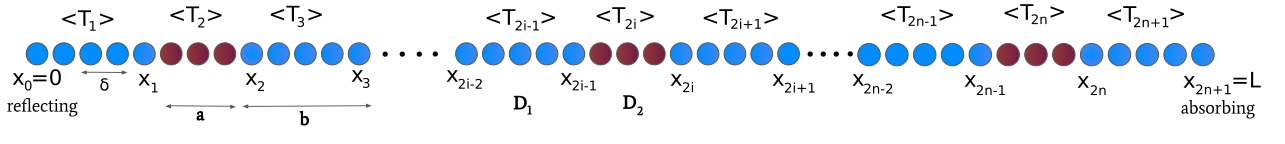
Figure 7: Schematic of the system with $n$ entropic barriers. The gap regions are denoted by blue and barriers are denoted by red. The boundary points of the $i^{th}$ barrier are denoted by $x_{2i-1}$ and $x_{2i}$. $\langle T_{i}\rangle$ denotes the mean average time for the particle to reach $x=L$ starting from the $i^{th}$ region.

The boundary points of $i^{th}$ barrier are denoted by $x_{2i-1}$ and $x_{2i}$ which can be expressed as

$$x_{2i-1} = b+(i-1)(a+b)~{}~{}~{}~{}~{}i\in(1,n)$$

$$x_{2i} = i(a+b)~{}~{}~{}~{}~{}~{}~{}~{}~{}~{}~{}~{}~{}~{}~{}~{}~{}~{}i\in(1,n)$$ (14)

The MFPT in two regions obey

$$D_{1}\frac{\partial^{2}\langle T_{2i-1}\rangle}{\partial x^{2}} = -1~{}~{}~{}~{}~{}~{}i\in(1,n+1)$$ (15)

$$D_{2}\frac{\partial^{2}\langle T_{2i}\rangle}{\partial x^{2}} = -1~{}~{}~{}~{}~{}~{}i\in(1,n)$$ (16)

which has solutions

$$\langle T_{2i-1}(x)\rangle = -\frac{1}{D_{1}}\left[\frac{x^{2}}{2}+A_{i}x+B_{i}\right]~{}~{}~{}~{}~{}~{}i\in(1,n+1)$$ (17)

$$\langle T_{2i}(x)\rangle = -\frac{1}{D_{2}}\left[\frac{x^{2}}{2}+C_{i}x+E_{i}\right]~{}~{}~{}~{}~{}~{}i\in(1,n)$$ (18)

where $A_{i},B_{i},C_{i},E_{i}$ are the integrating constants.
The boundary conditions of the lattice boundaries are given as,

$$\partial_{x}<T_{1}>_{x=0} = 0~{}~{}~{}~{}~{}~{}\rightarrow\mathit{reflecting~{}boundary}$$ (19)

$$<T_{2n+1}>_{x=L} = 0~{}~{}~{}~{}~{}~{}\rightarrow\mathit{absorbing~{}boundary}$$ (20)

The continuity MFPT at $x_{2i-1}$ and $x_{2i}$ gives,

$$\langle T_{2i-1}\rangle_{x_{2i-1}} = \langle T_{2i}\rangle_{x_{2i-1}}~{}~{}~{}~{}~{}~{}~{}~{}~{}~{}i\in(1,n)$$ (21)

$$\langle T_{2i}\rangle_{x_{2i}} = \langle T_{2i+1}\rangle_{x_{2i}}~{}~{}~{}~{}~{}~{}~{}~{}~{}~{}i\in(1,n)$$ (22)

Now the hopping dynamics that governs the motion can be written as,

$$\langle T_{2i-1}\rangle_{x_{2i-1}} = \frac{1}{p+q}+\frac{p}{p+q}\langle T_{2i-1}\rangle_{-\delta+x_{2i-1}}+\frac{q}{p+q}\langle T_{2i}\rangle_{\delta+x_{2i-1}}$$ (23)

$$\langle T_{2i+1}\rangle_{x_{2i}} = \frac{1}{p+q}+\frac{p}{p+q}\langle T_{2i+1}\rangle_{\delta+x_{2i}}+\frac{q}{p+q}\langle T_{2i}\rangle_{-\delta+x_{2i}}$$ (24)

Now from Eq.23 we can write,

$$(p+q)\langle T_{2i-1}\rangle_{x_{2i-1}} = 1+p\langle T_{2i-1}\rangle_{-\delta+x_{2i-1}}+q\langle T_{2i}\rangle_{\delta+x_{2i-1}}$$

$$\Rightarrow p\left[\langle T_{2i-1}\rangle_{x_{2i-1}}-\langle T_{2i-1}\rangle_{-\delta+x_{2i-1}}\right] = 1+q\left[\langle T_{2i}\rangle_{\delta+x_{2i-1}}-\langle T_{2i-1}\rangle_{x_{2i-1}}\right]$$

Using Eq.21 one can rewrite the above equation as,

$$p\left[\langle T_{2i-1}\rangle_{x_{2i-1}}-\langle T_{2i-1}\rangle_{-\delta+x_{2i-1}}\right] = 1+q\left[\langle T_{2i}\rangle_{\delta+x_{2i-1}}-\langle T_{2i}\rangle_{x_{2i-1}}\right]$$

$$p\delta\left[\langle T_{2i-1}\rangle_{x_{2i-1}}-\langle T_{2i-1}\rangle_{-\delta+x_{2i-1}}\right] = \delta+q\delta\left[\langle T_{2i}\rangle_{\delta+x_{2i-1}}-\langle T_{2i}\rangle_{x_{2i-1}}\right]$$

Now taking $\delta\rightarrow 0$ we get,

$$p\delta^{2}\partial_{x}\langle T_{2i-1}\rangle_{x_{2i-1}} = q\delta^{2}\partial_{x}\langle T_{2i}\rangle_{x_{2i-1}}$$

$$\Rightarrow D_{1}\partial_{x}\langle T_{2i-1}\rangle_{x_{2i-1}} = D_{2}\partial_{x}\langle T_{2i}\rangle_{x_{2i-1}}$$ (25)

Similarly from Eq.22 and Eq.24 one can write,

$$D_{2}\partial_{x}\langle T_{2i}\rangle_{x_{2i}} = D_{1}\partial_{x}<T_{2i+1}>_{x_{2i}}$$ (26)

Eqs.19,20,25 and 26 constitutes the boundary conditions for Eqs.17 and 18. From Eq.19 we have,

$$A_{1}=0$$ (27)

Now, using Eq.25 and Eq.26 respectively we have,

$$C_{i}=A_{i}$$ (28)

$$A_{i+1}=A_{i}$$ (29)

Combining the Eqs.27,29,28 we get,

$$A_{i}=C_{i}=0~{}~{}~{}~{}~{}~{}\forall i=\{1,n+1\}$$ (30)

Now from Eq.21 we have,

$$B_{i} = (s-1)\frac{x_{2i-1}^{2}}{2}+rE_{i}$$ (31)

where $s=D_{1}/D_{2}$.
Using Eq.22 we have,

$$B_{i+1}=(s-1)\frac{x_{2i}^{2}}{2}+sE_{i}$$ (32)

Combining Eqs.31 and 32 we get,

$$B_{i+1}=B_{i}+\frac{(s-1)}{2}\left[x_{2i}^{2}-x_{2i-1}^{2}\right]$$ (33)

Now from Eq.20 we have,

$$B_{n+1}=-\frac{x_{2n+1}^{2}}{2}=-\frac{L^{2}}{2}$$ (34)

Hence using Eq.33 we can write,

$$B_{1}=B_{n+1}-\frac{(s-1)}{2}\sum_{i=1}^{n}\left(x_{2i}^{2}-x_{2i-1}^{2}\right)$$ (35)

Therefore the MFPT of the particle to reach $x=L$ starting from $x=0$ in presence of $n$ barriers of width $a$ is given by,

$$\tau = \langle T_{1}\rangle_{x=0}=-\frac{B_{1}}{D_{1}}$$ (36)

$$= \frac{1}{D_{1}}\left[\frac{L^{2}}{2}+\frac{(s-1)}{2}\sum_{i=1}^{n}\left(x_{2i}^{2}-x_{2i-1}^{2}\right)\right]$$

The summation in the above equation can be computed very easily.

$$\sum_{i=1}^{n}\left(x_{2i}^{2}-x_{2i-1}^{2}\right) = \sum_{i=1}^{n}\left[i^{2}(a+b)^{2}-\{b+(i-1)(a+b)\}^{2}\right]$$ (37)

$$= \sum_{i=1}^{n}\left[i^{2}(a+b)^{2}-\{i(a+b)-a\}^{2}\right]$$

$$= \sum_{i=1}^{n}\left[2ia(a+b)-a^{2}\right]$$

$$= n(n+1)a(a+b)-na^{2}=naL$$

If $\tau_{0}$ denotes the MFPT of the particle in absence of barriers then we have

$$\tau_{0}=\frac{L^{2}}{2D_{1}}$$ (38)

Therefore the scaled MFPT in presence of barriers is given by,

$$\frac{\tau}{\tau_{0}} = \frac{2}{L^{2}}\left[\frac{L^{2}}{2}+\frac{(s-1)}{2}\sum_{i=1}^{n}\left(x_{2i}^{2}-x_{2i-1}^{2}\right)\right]$$ (39)

$$= 1+\frac{(s-1)}{L^{2}}\cdot naL$$

$$= 1+\frac{nr(s-1)}{(n+1)+nr}$$

where $r=a/b$.
 

II. Mean First Passage Time for energetic barriers

In the same spirit we shall now solve first passage time in case of energetic barriers. The hopping dynamics that determines the motion can be written as,

$$\langle T_{2i-1}\rangle_{x_{2i-1}} = \frac{1}{p+q}+\frac{p}{p+q}\langle T_{2i-1}\rangle_{-\delta+x_{2i-1}}+\frac{q}{p+q}\langle T_{2i+1}\rangle_{x_{2i}}$$

$$\therefore p\left(\langle T_{2i-1}\rangle_{x_{2i-1}}-\langle T_{2i-1}\rangle_{-\delta+x_{2i-1}}\right) = 1+q\langle T_{2i+1}\rangle_{x_{2i}}-q\langle T_{2i-1}\rangle_{x_{2i-1}}$$

$$\langle T_{2i-1}\rangle_{x_{2i-1}} = \frac{1}{q}+\langle T_{2i+1}\rangle_{x_{2i}}-\frac{p\delta}{q}\partial_{x}\langle T_{2i-1}\rangle_{x_{2i-1}}$$ (40)

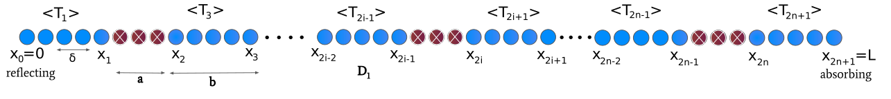
Figure 8: Schematic of the system with $n$ energetic barriers. The free regions are denoted by blue and barriers are denoted by red. The boundary points of the $i^{th}$ barrier are denoted by $x_{2i-1}$ and $x_{2i}$. $\langle T_{2i-1}\rangle$ denotes the mean time for the particle to reach $x=L$ starting from the $i^{th}$ free region. Note that in this case $\langle T_{2i}\rangle$’s do not exist for all values of $i$.

Now we define $D_{1}=p\delta^{2}$ and $v_{q}=q\delta$ such that both $D_{1}$ and $v_{q}$ are finite at $\delta\rightarrow 0$. Therefore we must have $p,q\rightarrow\infty$ and thus Eq.40 can be written as,

$$\langle T_{2i-1}\rangle_{x_{2i-1}}=\langle T_{2i+1}\rangle_{x_{2i}}-\frac{D_{1}}{v_{q}}\partial_{x}\langle T_{2i-1}\rangle_{x_{2i-1}}$$ (41)

Similarly it is easy to show that

$$\langle T_{2i-1}\rangle_{x_{2i-1}}=\langle T_{2i+1}\rangle_{x_{2i}}-\frac{D_{1}}{v_{q}}\partial_{x}\langle T_{2i+1}\rangle_{x_{2i}}$$ (42)

Hence from Eq.41 and Eq.42 we get,

$$\partial_{x}\langle T_{2i-1}\rangle_{x_{2i-1}}=\partial_{x}\langle T_{2i+1}\rangle_{x_{2i}}$$ (43)

For n energetic barriers, there will be n+1 fast regions where the particle diffuses. Therefore,

$$\langle T_{2i-1}\rangle=-\frac{1}{D_{1}}\left[\frac{x^{2}}{2}+A_{i}x+B_{i}\right]$$ (44)

where $i\in\{1,n+1\}$ denotes the region with boundaries $x_{2i-2}$ and $x_{2i-1}$ where the particle is in.
Now the lattice boundary conditions are same as Eq.19 and Eq.20,

$$\partial_{x}\langle T_{1}\rangle_{x=0}=0$$ (45)

$$\langle T_{2n+1}\rangle_{x=L}=0$$ (46)

Now Eq.45 gives

$$A_{1}=0$$

From Eq.43 we get,

$$A_{i+1}=A_{i}-a=A_{1}-ia=-ia$$ (47)

Using Eq.46 we find $B_{n+1}$ as,

$$B_{n+1}=-\frac{x_{2n+1}^{2}}{2}+nax_{2n+1}$$ (48)

where $x_{2n+1}=L=(n+1)(a+b)-a$.
Now from Eq.41 we can write,

$$B_{i}=B_{i+1}+\frac{1}{2}\left(x_{2i}^{2}-x_{2i-1}^{2}\right)+\left(A_{i+1}x_{2i}-A_{i}x_{2i-1}\right)-\frac{D_{1}}{v_{q}}\left[x_{2i}+A_{i+1}\right]$$ (49)

Therefore

$$B_{1} = B_{n+1}+\sum_{i=1}^{n}\frac{1}{2}\left(x_{2i}^{2}-x_{2i-1}^{2}\right)+\left(A_{i+1}x_{2i}-A_{i}x_{2i-1}\right)-\frac{D_{1}}{v_{q}}\left(x_{2i}+A_{i+1}\right)$$

$$\Rightarrow B_{1} = B_{n+1}-\frac{n(n-1)}{2}a^{2}+\frac{n(n+1)D_{1}a}{2v_{q}}-\frac{n(n+1)}{2}\left(\frac{D_{1}}{v_{q}}+a\right)(a+b)+\frac{1}{2}\sum_{i=1}^{n}\left(x_{2i}^{2}-x_{2i-1}^{2}\right)$$

Using Eq.14, Eq.37 and Eq.48, we can easily show from Eq.LABEL:eq:B1 that

$$B_{1}=-\frac{(n+1)^{2}b^{2}+n(n+1)\frac{D_{1}b}{v_{q}}}{2}$$ (51)

The scaled first passage passage time then can be written as,

$$\frac{\tau}{\tau_{0}}=-\frac{2B_{1}}{L^{2}} = \frac{(n+1)^{2}b^{2}+n(n+1)\frac{D_{1}b}{v_{q}}}{L^{2}}$$

Now using the relation $L=(n+1)(a+b)-a=n(a+b)+b$ one can write,

$$\frac{\tau}{\tau_{0}} = \frac{\frac{(L+a)^{2}}{(a+b)^{2}}b^{2}+\left(\frac{L-b}{a+b}\right)\left(\frac{L+a}{a+b}\right)\frac{D_{1}b}{v_{q}}}{L^{2}}$$ (52)

$$= \frac{\frac{b^{2}(L+a)^{2}}{(a+b)^{2}}+\frac{(L^{2}+aL-bL-ab)}{(a+b)^{2}}\frac{D_{1}b}{v_{q}}}{L^{2}}$$

$$= \frac{\frac{b^{2}(L+a)^{2}}{L^{2}}+\frac{(L^{2}+aL-bL-ab)}{L^{2}}\frac{D_{1}b}{v_{q}}}{(a+b)^{2}}$$

$$= \frac{b^{2}\left(1+\frac{a}{L}\right)^{2}+\left(1+\frac{a}{L}-\frac{b}{L}-\frac{ab}{L^{2}}\right)\frac{D_{1}b}{v_{q}}}{(a+b)^{2}}$$

$$= \frac{b^{2}\left(1+\frac{a}{L}\right)^{2}+\left(\frac{L}{b}+\frac{a}{b}-1-\frac{a}{L}\right)\frac{D_{1}b^{2}}{Lv_{q}}}{(a+b)^{2}}$$

$$= \frac{b^{2}\left(1+\frac{a}{L}\right)^{2}+\left[\frac{a}{b}\left(\frac{L}{a}+1\right)-\frac{a}{L}\left(\frac{L}{a}+1\right)\right]\frac{D_{1}b^{2}}{Lv_{q}}}{b^{2}\left(1+\frac{a}{b}\right)^{2}}$$

$$= \frac{\left(1+\frac{a}{L}\right)^{2}+\left(r-\frac{a}{L}\right)\left(1+\frac{L}{a}\right)\frac{D}{Lv_{q}}}{(1+r)^{2}}$$

where again $r=a/b$.

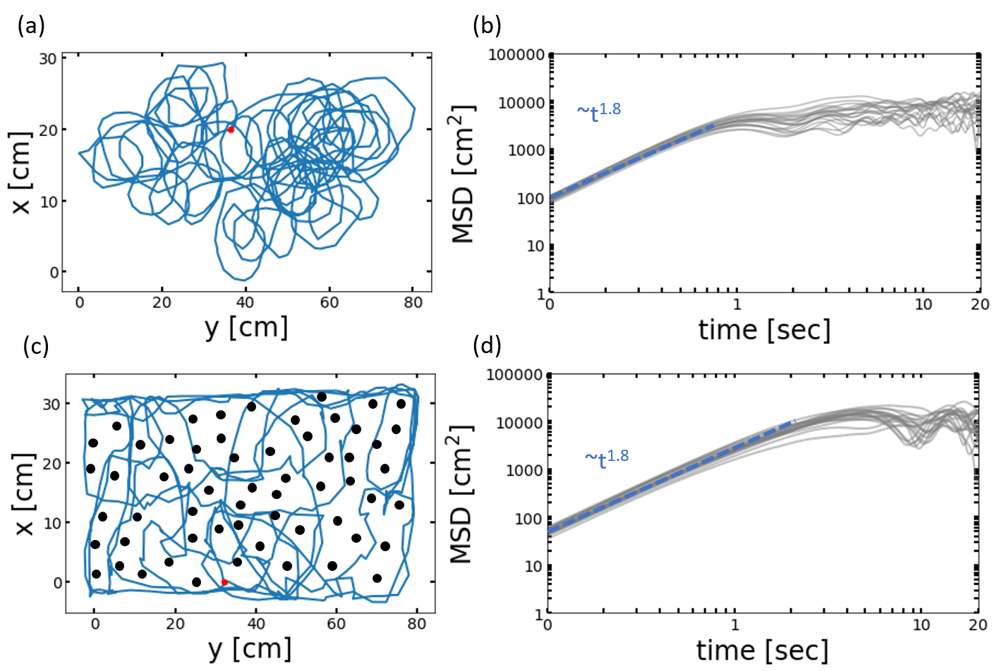
Figure 9: (a) Sample trajectory of RW in empty region of dimensions 76 $\times$ 27$cm$. (b) Mean square displacement corresponding to (a) shows superdiffusive behavior in first 1 second which becomes subdiffusive at long times (due to combination of circling and presence of boundary). (c) Sample trajectory through obstacles of diameter 1 cm in a region of width 76 $\times$ 27 $cm$. (d) Mean square displacement corresponding to (c) shows an initial superdiffusive behavior for a longer period than (a) which becomes subdiffusive at long times, similar to panel (b).

.

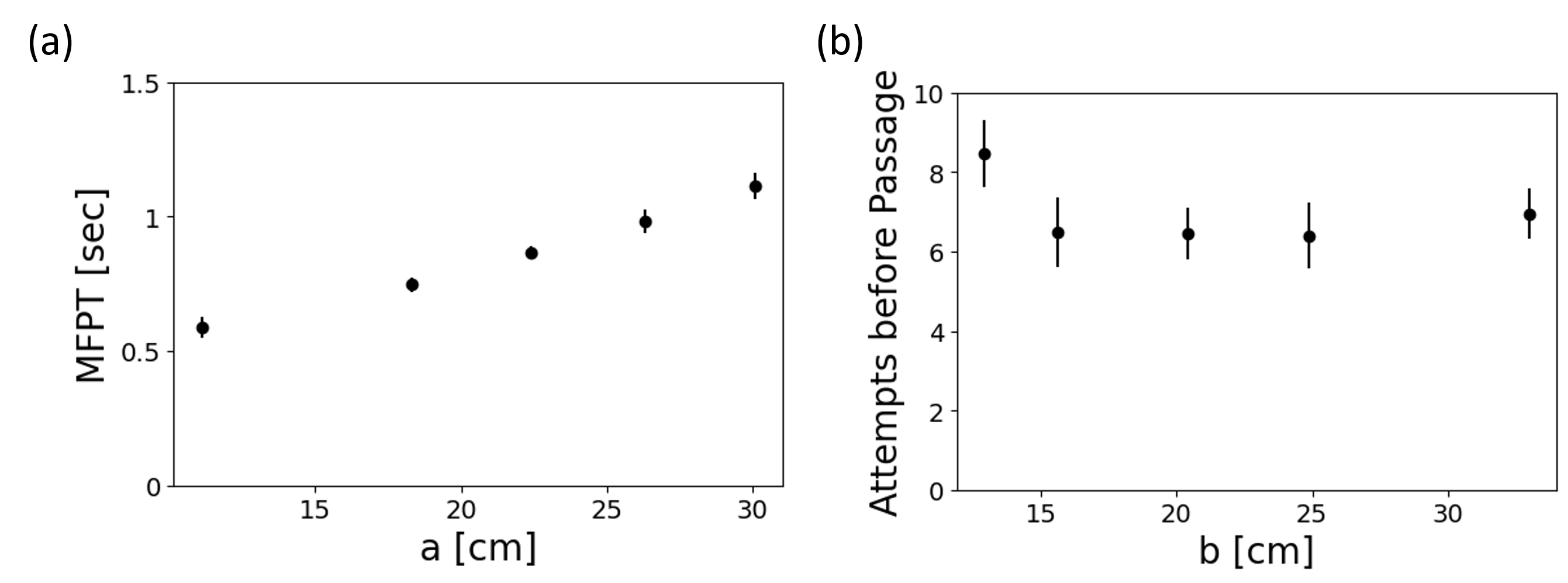
Figure 10: (a) Mean First Passage Time (MFPT) to traverse the barrier (tunnel) regions for the case of energetic barrier. The times increase roughly linearly with the width of the barrier region, indicating ballistic transport through the tunnels, as expected. (b) The number of times the RW collides with the barrier interface before it successfully enters the barrier (tunnel) region for the case of energetic barriers. This is a intrinsic property of the barrier, and is experimentally seems to be independent of the width of the barrier regions, as expected.

References

- Gardiner et al. [1985] C. W. Gardiner et al., Handbook of stochastic methods, Vol. 3 (springer Berlin, 1985).
- Redner [2001] S. Redner, A guide to first-passage processes (Cambridge university press, 2001).
- Metzler and Klafter [2004] R. Metzler and J. Klafter, The restaurant at the end of the random walk: recent developments in the description of anomalous transport by fractional dynamics, Journal of Physics A: Mathematical and General 37, R161 (2004).
- Bénichou et al. [2011] O. Bénichou, C. Loverdo, M. Moreau, and R. Voituriez, Intermittent search strategies, Reviews of Modern Physics 83, 81 (2011).
- Klumpp and Lipowsky [2005] S. Klumpp and R. Lipowsky, Cooperative cargo transport by several molecular motors, Proceedings of the National Academy of Sciences 102, 17284 (2005).
- Müller et al. [2008] M. J. Müller, S. Klumpp, and R. Lipowsky, Tug-of-war as a cooperative mechanism for bidirectional cargo transport by molecular motors, Proceedings of the National Academy of Sciences 105, 4609 (2008).
- Bressloff and Newby [2013] P. C. Bressloff and J. M. Newby, Stochastic models of intracellular transport, Reviews of Modern Physics 85, 135 (2013).
- Roldán et al. [2016] É. Roldán, A. Lisica, D. Sánchez-Taltavull, and S. W. Grill, Stochastic resetting in backtrack recovery by rna polymerases, Physical Review E 93, 062411 (2016).
- Guthold et al. [1999] M. Guthold, X. Zhu, C. Rivetti, G. Yang, N. H. Thomson, S. Kasas, H. G. Hansma, B. Smith, P. K. Hansma, and C. Bustamante, Direct observation of one-dimensional diffusion and transcription by escherichia coli rna polymerase, Biophysical journal 77, 2284 (1999).
- Sahoo and Klumpp [2013] M. Sahoo and S. Klumpp, Backtracking dynamics of rna polymerase: pausing and error correction, Journal of Physics: Condensed Matter 25, 374104 (2013).
- Maji et al. [2020] A. Maji, R. Padinhateeri, and M. K. Mitra, The accidental ally: Nucleosome barriers can accelerate cohesin-mediated loop formation in chromatin, Biophysical journal 119, 2316 (2020).
- Davidson et al. [2019] I. F. Davidson, B. Bauer, D. Goetz, W. Tang, G. Wutz, and J.-M. Peters, Dna loop extrusion by human cohesin, Science 366, 1338 (2019).
- Banigan and Mirny [2020] E. J. Banigan and L. A. Mirny, Loop extrusion: theory meets single-molecule experiments, Current opinion in cell biology 64, 124 (2020).
- Ganji et al. [2018] M. Ganji, I. A. Shaltiel, S. Bisht, E. Kim, A. Kalichava, C. H. Haering, and C. Dekker, Real-time imaging of dna loop extrusion by condensin, Science 360, 102 (2018).
- Banigan et al. [2020] E. J. Banigan, A. A. van den Berg, H. B. Brandão, J. F. Marko, and L. A. Mirny, Chromosome organization by one-sided and two-sided loop extrusion, Elife 9, e53558 (2020).
- Golfier et al. [2020] S. Golfier, T. Quail, H. Kimura, and J. Brugués, Cohesin and condensin extrude dna loops in a cell cycle-dependent manner, Elife 9, e53885 (2020).
- Goloborodko et al. [2016] A. Goloborodko, M. V. Imakaev, J. F. Marko, and L. Mirny, Compaction and segregation of sister chromatids via active loop extrusion, Elife 5, e14864 (2016).
- Kolomeisky [2011] A. B. Kolomeisky, Physics of protein–dna interactions: mechanisms of facilitated target search, Physical Chemistry Chemical Physics 13, 2088 (2011).
- van Zon et al. [2006] J. S. van Zon, M. J. Morelli, S. Tǎnase-Nicola, and P. R. ten Wolde, Diffusion of transcription factors can drastically enhance the noise in gene expression, Biophysical journal 91, 4350 (2006).
- Souza et al. [2015] R. Souza, A. Ambrosini, and L. M. Passaglia, Plant growth-promoting bacteria as inoculants in agricultural soils, Genet. Mol. Biol 38, 401 (2015).
- Watt and Passioura [2006] J. Watt, M.and Kirkegaard and J. Passioura, Rhizosphere biology and crop productivity—a review, Soil Res. 44, 299 (2006).
- Bhattacharjee and Dutta [2019] T. Bhattacharjee and S. Dutta, Bacterial hopping and trapping in porous media, Nature Communications 10, 2075 (2019).
- Dix and Verkman [2008] J. A. Dix and A. Verkman, Crowding effects on diffusion in solutions and cells, Annu. Rev. Biophys. 37, 247 (2008).
- Goychuk et al. [2014] I. Goychuk, V. O. Kharchenko, and R. Metzler, How molecular motors work in the crowded environment of living cells: coexistence and efficiency of normal and anomalous transport, PloS one 9, e91700 (2014).
- Jin et al. [2010] J. Jin, L. Bai, D. S. Johnson, R. M. Fulbright, M. L. Kireeva, M. Kashlev, and M. D. Wang, Synergistic action of rna polymerases in overcoming the nucleosomal barrier, Nature structural & molecular biology 17, 745 (2010).
- Kireeva et al. [2005] M. L. Kireeva, B. Hancock, G. H. Cremona, W. Walter, V. M. Studitsky, and M. Kashlev, Nature of the nucleosomal barrier to rna polymerase ii, Molecular cell 18, 97 (2005).
- Stigler et al. [2016] J. Stigler, G. Camdere, D. Koshland, and E. Greene, Single-molecule imaging reveals a collapsed conformational state for dna-bound cohesin, Cell Reports 15, 988 (2016).
- Daniels et al. [2012] B. R. Daniels, R. Rikhy, M. Renz, T. M. Dobrowsky, and J. Lippincott-Schwartz, Multiscale diffusion in the mitotic drosophila melanogaster syncytial blastoderm, Proceedings of the National Academy of Sciences 109, 8588 (2012).
- Rikhy et al. [2015] R. Rikhy, M. Mavrakis, and J. Lippincott-Schwartz, Dynamin regulates metaphase furrow formation and plasma membrane compartmentalization in the syncytial drosophila embryo, Biology open 4, 301 (2015).
- Bénichou and Voituriez [2014] O. Bénichou and R. Voituriez, From first-passage times of random walks in confinement to geometry-controlled kinetics, Physics Reports 539, 225 (2014).
- Chou and D’Orsogna [2014] T. Chou and M. R. D’Orsogna, First passage problems in biology, in First-passage phenomena and their applications (World Scientific, 2014) pp. 306–345.
- Iyer-Biswas and Zilman [2016] S. Iyer-Biswas and A. Zilman, First-passage processes in cellular biology, Advances in chemical physics 160, 261 (2016).
- Bray et al. [2013] A. J. Bray, S. N. Majumdar, and G. Schehr, Persistence and first-passage properties in nonequilibrium systems, Advances in Physics 62, 225 (2013).
- Kalinina et al. [2013] I. Kalinina, A. Nandi, P. Delivani, M. R. Chacón, A. H. Klemm, D. Ramunno-Johnson, A. Krull, B. Lindner, N. Pavin, and I. M. Tolić-Nørrelykke, Pivoting of microtubules around the spindle pole accelerates kinetochore capture, Nature cell biology 15, 82 (2013).
- Nayak et al. [2020] I. Nayak, D. Das, and A. Nandi, Comparison of mechanisms of kinetochore capture with varying number of spindle microtubules, Physical Review Research 2, 013114 (2020).
- Parmar et al. [2016] J. Parmar, D. Das, and R. Padinhateeri, Theoretical estimates of exposure timescales of protein binding sites on dna regulated by nucleosome kinetics, Nucleic Acids Research 44, 1630–1641 (2016).
- Ghusinga et al. [2017] K. Ghusinga, D. J.J, and A. Singh, First-passage time approach to controlling noise in the timing of intracellular events, PNAS 114, 693 (2017).
- Rijal et al. [2020] K. Rijal, A. Prasad, and D. Das, Protein hourglass: Exact first passage time distributions for protein thresholds, Phys. Rev. E 102, 052413 (2020).
- Rijal et al. [2022] K. Rijal, A. Prasad, A. Singh, and D. Das, Exact distribution of threshold crossing times for protein concentrations: Implication for biological timekeeping, Phys. Rev. Lett. 128, 048101 (2022).
- Iyer-Biswas et al. [2014] S. Iyer-Biswas, C. Wright, J. Henry, K. Lo, S. Burov, Y. Lin, G. Crooks, S. Crosson, A. Dinner, and N. Scherer, Scaling laws governing stochastic growth and division of single bacterial cells, PNAS 111, 15912 (2014).
- Makarchuk et al. [2019] S. Makarchuk, V. Braz, N. Araujo, L. Ciric, and G. Volpe, Enhanced propagation of motile bacteria on surfaces due to forward scattering, Nature Communications 10, 4110 (2019).
- Frangipane et al. [2019] G. Frangipane, G. Vizsnyiczai, C. Maggi, R. Savo, A. Sciortino, S. Gigan, and R. Leonardo, Invariance properties of bacterial random walks in complex structures, Nature Communications 10, 2442 (2019).
- Biswas et al. [2020] A. Biswas, J. Cruz, P. Paramananda, and D. Das, First passage of an active particle in the presence of passive crowders, Soft Matter 16, 6138 (2020).
- Hänggi et al. [1990] P. Hänggi, P. Talkner, and M. Borkovec, Reaction-rate theory: fifty years after kramers, Reviews of modern physics 62, 251 (1990).
- Reguera et al. [2006] D. Reguera, G. Schmid, P. S. Burada, J. Rubi, P. Reimann, and P. Hänggi, Entropic transport: Kinetics, scaling, and control mechanisms, Physical review letters 96, 130603 (2006).
- Baumgärtner and Muthukumar [1987] A. Baumgärtner and M. Muthukumar, A trapped polymer chain in random porous media, J. Chem. Phys. 87, 3082 (1987).
- Muthukumar and Baumgärtner [1989] M. Muthukumar and A. Baumgärtner, Effects of entropic barriers on polymer dynamics, Macromolecules 22, 1937 (1989).
- Majumdar et al. [2004] S. Majumdar, D. Das, J. Kondev, and B. Chakraborty, Landau-like theory of glassy dynamics, Phys. Rev. E 70, 060501 (2004).
- Garnett [1904] J. M. Garnett, Xii. colours in metal glasses and in metallic films, Philosophical Transactions of the Royal Society of London. Series A, Containing Papers of a Mathematical or Physical Character 203, 385 (1904).
- Kalnin and Kotomin [2012] J. R. Kalnin and E. Kotomin, Note: Effective diffusion coefficient in heterogeneous media, The Journal of Chemical Physics 137, 166101 (2012).
- Schütz and Trimper [2004] G. M. Schütz and S. Trimper, Elephants can always remember: Exact long-range memory effects in a non-markovian random walk, Physical Review E 70, 045101 (2004).
- Reverey et al. [2015] J. F. Reverey, J.-H. Jeon, H. Bao, M. Leippe, R. Metzler, and C. Selhuber-Unkel, Superdiffusion dominates intracellular particle motion in the supercrowded cytoplasm of pathogenic acanthamoeba castellanii, Scientific reports 5, 1 (2015).
- Righini et al. [2018] M. Righini, A. Lee, C. Cañari-Chumpitaz, T. Lionberger, R. Gabizon, Y. Coello, I. Tinoco Jr, and C. Bustamante, Full molecular trajectories of rna polymerase at single base-pair resolution, Proceedings of the National Academy of Sciences 115, 1286 (2018).
- Rai et al. [2013] A. K. Rai, A. Rai, A. J. Ramaiya, R. Jha, and R. Mallik, Molecular adaptations allow dynein to generate large collective forces inside cells, Cell 152, 172 (2013).
- Pradhan et al. [2022] B. Pradhan, R. Barth, E. Kim, I. F. Davidson, B. Bauer, T. van Laar, W. Yang, J.-K. Ryu, J. van der Torre, J.-M. Peters, et al., Smc complexes can traverse physical roadblocks bigger than their ring size, Cell Reports 41, 111491 (2022).
Acknowledgements
We thank Kong Yang for help with preliminary data collection. M.D. acknowledges American Association of University Women (AAUW) Research Publication Grant in Engineering, Medicine and Science’21 for funding experimental aspects of this research. D.D. acknowledges SERB India (Grant No. MTR/2019/000341) for supporting this work. M.K.M and S.G. acknowledge computing support from IIT Bombay.