Late lumping of observer-based state feedback for boundary control systems

Abstract

Infinite-dimensional linear systems with unbounded input and output operators are considered. For the purpose of finite-dimensional observer-based state feedback, an observer approximation scheme will be developed which can be directly combined with existing late-lumping controllers and observer output injection gains. It relies on a decomposition of the feedback gain, resp. observer output injection gain, into a bounded and an unbounded part. Based on a perturbation result, the spectrum-determined growth condition is established, for the closed loop.

1 Introduction

Infinite-dimensional linear systems with unbounded input and output operators are considered. The purpose of the article is to combine feedback gain and observer gain approximations to finite-dimensional observer-based state feedback (FOSF). Therefore, this article addresses the approximation of the observer. Previous results in this direction come e.g. from (Deutscher, 2013; Grüne and Meurer, 2022; Curtain, 1984).

Using the perturbation result from Xu and Sallet (1996), it will be proven that the closed-loop system is a discrete Riesz-spectral (RS) system. Hence, the stability can be checked by computing the eigenvalues of the closed-loop operator. To the authors’ knowledge, this is the first proof in this context, which covers both analytic and hyperbolic systems. For analytic systems Curtain (1984) has proven a similar result, using a perturbation result from Kato (1995).

The article is organized as follows. In Section 2 the system class will be introduced. In Section 3 the structure of the observer, and the feedback and observer gain approximations will be stated. In Section 4 the approximation scheme for the observer will be derived. Section 5 summarizes the article.

2 Preliminaries

Within this section the notation and the structural properties of the systems and designs under consideration will be introduced.

2.1 Basic notation

The complex conjugate of a complex number $c\in\mathbb{C}$ is denoted by $\overline{c}$. Moreover, $L^{2}(a,b;\mathbb{C}^{n})$ denotes the Lebesgue space of square-integrable functions $f:[a,b]\to\mathbb{C}^{n}$, $z\mapsto f(z)$, while $H^{n}(a,b;\mathbb{C}^{n})$ is the usual Sobolev space of $n$ times weakly differentiable (in $L^{2}(a,b;\mathbb{C}^{n})$) functions on $[a,b]$ taking values in $\mathbb{C}^{n}$.

The partial derivative of order $n\in\mathbb{N}$ w.r.t. a variable $z$ is denoted by $\partial_{z}^{n}$. Throughout this paper, $t\in\mathbb{R}$ stands exclusively for the time variable, the first (partial) derivative w.r.t. $t$ of a function $h$ is abbreviated by $\dot{h}$. For two Banach spaces $\mathcal{M}$ and $\mathcal{N}$, $\mathscr{L}(\mathcal{M},\mathcal{N})$ denotes the Banach space of linear bounded operators $\mathcal{M}\to\mathcal{N}$.

Let $\mathcal{X}$ denote a separable Hilbert space and $\mathcal{A}:\mathcal{X}\rightarrow\mathcal{X}$ a linear operator, which is not necessarily bounded on $\mathcal{X}$. The spectrum and the point spectrum of $\mathcal{A}$ are denoted by $\sigma(\mathcal{A})$ and $\sigma_{p}(\mathcal{A})$, respectively. Furthermore, $\{\lambda_{i}\}$ denotes the sequence of eigenvalues of $\mathcal{A}$ and $\{\varphi_{i}\}$ the corresponding sequence of eigenvectors. The adjoint operator of $\mathcal{A}$ is denoted by $\mathcal{A}^{*}$, with eigenvalues $\{\lambda_{i}^{*}\}$ and eigenvectors $\{\varphi_{i}^{*}\}$. The resolvent of $\mathcal{A}$ is denoted by $R(\mathcal{A},\lambda)=(\lambda I-\mathcal{A})^{-1}$, $\lambda\not\in\sigma(\mathcal{A})$, with $I$ the identity. Moreover, $D(\mathcal{A})$ is the domain of $\mathcal{A}$ and $D(\mathcal{A})^{\prime}$ is the dual space of $D(\mathcal{A})$. These spaces are equipped with the graph norm and the corresponding dual norm, respectively. The duality pairing in $D(\mathcal{A}^{*})$ is denoted by $\langle F,g\rangle_{D(\mathcal{A}^{*})},\,F\in D(\mathcal{A}^{*})^{\prime},\,g\in D(\mathcal{A}^{*})$ and the scalar product in $\mathcal{X}$ is denoted by $\langle f,g\rangle_{\mathcal{X}},\,f,g\in\mathcal{X}$. The scalar product as well as the duality pairing take complex conjugation on the second argument. The space of square-summable sequences and the space of bounded sequences are denoted by $l^{2}$ and $l^{\infty}$, respectively. Finally, $\delta_{r}(\cdot)$ is the Dirac delta distribution centered in $r\in\mathbb{R}$.

2.2 System structure

Boundary control systems (Fattorini, 1968) with boundary observation are considered. They are of the form

$$\dot{x}(t) =\mathfrak{A}x(t), x(0)=x_{0}\in\mathcal{X}$$ (1a)

$$u(t) =\mathfrak{R}x(t)$$ (1b)

$$y(t) =\mathfrak{C}x(t)$$ (1c)

with state $x(t)\in\mathcal{X}$, input $u(t)\in\mathcal{U}=\mathbb{C}$ and output $y(t)\in\mathcal{Y}=\mathbb{C}$, cf. (Fattorini, 1968). The state space $\mathcal{X}$ is a separable Hilbert space and $\mathfrak{A}:\mathcal{X}\supset D(\mathfrak{A})\rightarrow\mathcal{X}$, $\mathfrak{R}:\mathcal{X}\supset D(\mathfrak{A})\rightarrow\mathcal{U}$ and $\mathfrak{C}:\mathcal{X}\supset D(\mathfrak{A})\rightarrow\mathcal{Y}$ are unbounded operators on $\mathcal{X}$.

It is convenient to consider (1) also in the form

$$(\dot{x}(t),y(t)) =\Sigma\left(x(t),u(t)\right), x(0)=x_{0}\in\mathcal{X},$$ (2)

where $\Sigma:\mathcal{X}\times\mathcal{U}\supset D(\Sigma)\rightarrow\mathcal{X}\times\mathcal{Y}$ is unbounded and $D(\Sigma)=\{(h_{x},h_{u})\in D(\mathfrak{A})\times\mathcal{U}\,|\,\mathfrak{R}h_{x}=h_{u}\}$ is dense in $\mathcal{X}\times\mathcal{U}$.

System (1) (resp. (2)) is called a system with boundary observation (BOS), if the adjoint system

$$\left(\dot{x}^{*}(t),u^{*}(t)\right)=\Sigma^{*}\left(x^{*}(t),y^{*}(t)\right)$$ (3)

with input $y^{*}(t)\in\mathcal{Y}$ and output $u^{*}(t)\in\mathcal{U}$ is a boundary control system (BCS), i.e., there exist operators

$$\mathscr{A}:D(\mathscr{A})\to\mathcal{X}, \mathscr{R}:D(\mathscr{A})\to\mathcal{Y}, \mathscr{C}:D(\mathscr{A})\to\mathcal{U}$$

with similar properties as $\mathfrak{A}$, $\mathfrak{R}$, $\mathfrak{C}$ such that

$$\Sigma^{*}(x^{*}(t),y^{*}(t))=(\mathscr{A}x^{*}(t),\mathscr{C}x^{*}(t)),\\ D(\Sigma^{*})=\{(h_{x^{*}},h_{y^{*}})\in D(\mathscr{A})\times\mathcal{Y}\,|\,\mathscr{R}h_{x^{*}}=h_{y^{*}}\}.$$

For a unified treatment of the controller and observer design, a reformulation of (2) (resp. (1)) as evolution equation

$$\dot{x}(t) =\mathcal{A}x(t)+\mathcal{B}u(t), x(0)=x_{0}\in\mathcal{X},$$ (4a)

as described in (Bensoussan et al., 2007, Chapter 3), is considered. Therein, the system operator $\mathcal{A}:\mathcal{X}\supset D(\mathcal{A})\rightarrow\mathcal{X}$ and the input operator $\mathcal{B}\in\mathscr{L}(\mathcal{U},D(\mathcal{A}^{*})^{\prime})$ are defined by the following relations:

$$D(\mathcal{A})=\{h\in D(\mathfrak{A})\,|\,\mathfrak{R}h=0\}$$ (5a)

$$\mathcal{A}h=\mathfrak{A}h, \forall\,h\!\in\!D(\mathcal{A})$$ (5b)

$$\langle\mathcal{B},h\rangle_{D(\mathcal{A}^{*})}=\langle\left(0,1\right),\Sigma^{*}(h,0)\rangle_{\mathcal{X}\times\mathcal{U}}, \forall\,h\!\in\!D(\mathcal{A}^{*}).$$ (5c)

Similarly, the adjoint system (3) is associated with

$$\dot{x}^{*}(t) =\mathcal{A}^{*}x^{*}(t)+\mathcal{C}^{*}y^{*}(t), x^{*}(0)=x^{*}_{0}\in\mathcal{X}$$ (6a)

where

$$D(\mathcal{A}^{*})=\{h\in D(\mathscr{A})\,|\,\mathscr{R}h=0\}$$

$$\mathcal{A}^{*}h=\mathscr{A}h, \forall\,h\in D(\mathcal{A}^{*})$$

$$\langle\mathcal{C}^{*},h\rangle_{D(\mathcal{A})}=\langle\left(0,1\right),\Sigma(h,0)\rangle_{\mathcal{X}\times\mathcal{Y}}, \forall\,h\in D(\mathcal{A}).$$

While $y(t)=\mathcal{C}x(t)=\langle\mathcal{C}^{*},x(t)\rangle_{D(\mathcal{A})}$ holds for the autonomous system ($u(t)=0$), for the actuated system $y(t)\neq\mathcal{C}x(t)$ in general case, compare (Weiss, 1994). Therefore, throughout this paper the output equation (1c) is used to determine the output of the system.

Throughout this contribution, $\mathcal{A}$ is assumed to be the infinitesimal generator of a $\text{C}_{0}$-semigroup on $\mathcal{X}$, while both $\mathcal{B}$ and $\mathcal{C}^{*}$ are not required to be admissible in the sense of (Tucsnak and Weiss, 2009).

2.2.1 Example system.

The following example system will be used in Section 4 for the application of the proposed approximation scheme. Therefore, for this example, in Section 3 also the corresponding feedback, observer gain and observer approximations are given.

Consider the hyperbolic system

$$\begin{split}\partial_{t}w_{1}(z,t)&=\alpha\partial_{z}w_{2}(z,t)\end{split}$$ (7a)

$$\begin{split}\partial_{t}w_{2}(z,t)&=\beta\partial_{z}w_{1}(z,t)\end{split}$$ (7b)

$$\begin{split}\partial_{t}w_{3}(t)&=\gamma w_{2}(0,t)\end{split}$$ (7c)

with boundary conditions (BCs)

$$w_{3}(t)=w_{1}(0,t), u(t)=w_{2}(1,t),$$ (7d)

input $u(t)$, and output $y(t)=w_{1}(1,t)$. This model can be used to describe the linearized dynamics of an undamped pneumatic system (Gehring and Kern, 2018). With state

$$x(t)=(w_{1}(\cdot,t),w_{2}(\cdot,t),w_{3}(t))\in\mathcal{X}=L^{2}(0,1;\mathbb{C}^{2})\times\mathbb{C},$$

(7) can be written in the form (1) with $\mathfrak{R}h\!=\!h_{2}(1)$, $\mathfrak{C}h\!=\!h_{1}(1)$, $\mathfrak{A}h\!=\!(\alpha\partial_{z}h_{2},\,\beta\partial_{z}h_{1},\,\gamma h_{2}(0))$, $(h_{1},h_{2},h_{3})\in D(\mathfrak{A})$,

$$D(\mathfrak{A})\! =\!\{(h_{1},h_{2},h_{3})\!\in\!\mathcal{X}|\partial_{z}h_{1},\partial_{z}h_{2}\!\in\!L^{2}(0,1),h_{3}\!=\!h_{1}(0)\}$$

or in state space representation (4) with $\mathcal{B}=(\alpha\,\delta_{1}(\cdot),0,0)$,

$$\mathcal{A}\,h =\mathfrak{A}\,h,\,\,h\in D(\mathcal{A})=\{(h_{1},h_{2},h_{3})\in D(\mathfrak{A})\,|\,h_{2}(1)=0\}.$$

3 Design and approximation

The aim of the paper is to connect the approximation schemes, proposed in (Riesmeier and Woittennek, 2022), for state feedback and observer output-injection, to an approximation scheme for FOSF. Therefore, the basic approximation schemes from there will be briefly summarized in the following. Based on this, a representation of the observer will be derived, which serves as the basis for the approximation in Section 4.

3.1 Feedback design and approximation

As described in (Riesmeier and Woittennek, 2022) the control law

$$u(t)=\breve{\mathfrak{K}}x(t)+\varkappa\,u^{\text{\rm{dc}}}(t),$$

with arbitrary non-zero $\varkappa\in\mathbb{R}$ and feedback gain

$$\breve{\mathfrak{K}}=\mathfrak{R}-\varkappa\mathfrak{R}^{\text{\rm{dc}}},$$

assigns the desired dynamics $\mathcal{A}^{\text{\rm{dc}}}$ to the closed loop

$$\dot{x}(t) =\mathfrak{A}x(t), x(0)=x_{0}\in\mathcal{X}$$ (8a)

$$u^{\text{\rm{dc}}}(t) =\mathfrak{R}^{\text{\rm{dc}}}x(t)$$ (8b)

$$y(t) =\mathfrak{C}x(t).$$ (8c)

For the BCS $(\mathfrak{A},\mathfrak{R}^{\text{\rm{dc}}},\mathfrak{C})$ the system operators $(\Sigma^{\text{\rm{dc}}},\mathcal{A}^{\text{\rm{dc}}},$ $\mathcal{B}^{\text{\rm{dc}}})$ can be derived in the same way as $({\Sigma},{\mathcal{A}},{\mathcal{B}})$ are derived from $(\mathfrak{A},{\mathfrak{R}},\mathfrak{C})$, c.f. Section 2.2.

Since only the bounded part of the feedback is subject to approximation, the feedback gain requires a decomposition

$$u(t)=\mathring{\mathfrak{K}}x(t)+\mathcal{K}x(t)+\varkappa\,u^{\text{\rm{dc}}}(t)$$ (9)

into an unbounded part $\mathring{\mathfrak{K}}\in\mathscr{L}(D(\mathfrak{A}),\mathcal{U})$ and a bounded part $\mathcal{K}\in\mathscr{L}(\mathcal{X},\mathcal{U})$. Therewith, the controller intermediate system

$$\dot{x}(t) =\mathfrak{A}x(t), x(0)=x_{0}\in\mathcal{X}$$ (10a)

$$u^{\text{\rm{c}}}(t) =\mathfrak{R}^{\text{\rm{c}}}x(t), \mathfrak{R}^{\text{\rm{c}}}=\mathfrak{R}-\mathring{\mathfrak{K}}$$ (10b)

$$y(t) =\mathfrak{C}x(t)$$ (10c)

can be introduced by defining the respective input by

$$u^{\text{\rm{c}}}(t)=\mathcal{K}x(t)+\varkappa\,u^{\text{\rm{dc}}}(t).$$

As described above, the controller intermediate system operators $(\Sigma^{\text{\rm{c}}},\mathcal{A}^{\text{\rm{c}}},\mathcal{B}^{\text{\rm{c}}})$ can be derived from $(\mathfrak{A},\mathfrak{R}^{\text{\rm{c}}},\mathfrak{C})$.

For the results of this article, approximations with respect to the eigenvectors $\{\varphi^{\text{\rm{o}}}_{1}\}_{1}^{n}$ and $\{\varphi^{\text{\rm{o}}*}_{1}\}_{1}^{n}$ of $\mathcal{A}^{\text{\rm{o}}}$ resp. $\mathcal{A}^{\text{\rm{o}}*}$ (to be introduced in the next subsection), are considered. As described in (Riesmeier and Woittennek, 2022) $\mathcal{K}$ can now be approximated:

$$\mathcal{K}^{n} =\sum_{i=1}^{n}\langle\cdot,\varphi^{\text{\rm{o}}*}_{i}\rangle_{\mathcal{X}}\,k^{\text{\rm{o}}}_{i}\,\in\,\mathscr{L}(\mathcal{X},\mathcal{U}), k^{\text{\rm{o}}}_{i}=\mathcal{K}\varphi^{\text{\rm{o}}}_{i}.$$ (11)

3.1.1 State-feedback approximation for the example system.

According to (Riesmeier and Woittennek, 2022), the feedback gain which assigns the desired dynamics of the delay differential equation

$$\dot{\chi}(t+\tau)+\mu_{\text{c}}\,\dot{\chi}(t-\tau)+\kappa_{\text{c}}(\chi(t+\tau)+\mu_{\text{c}}\,\chi(t-\tau))=0,$$

to the closed loop (approximately), is given by $u(t)=\mathring{\mathfrak{K}}x(t)+\mathcal{K}^{n}x(t)$, where the unbounded part is reads

$$\mathring{\mathfrak{K}}h=\frac{\beta\tau(\mu_{\text{c}}-1)}{\mu_{\text{c}}+1}h_{1}(1), h=(h_{1},h_{2},h_{3})\in D(\mathfrak{A})$$

and the bounded part $\mathcal{K}^{n}$, defined by (11), is completed by the gains $\{k^{\text{\rm{o}}}_{i}=\varphi^{\text{\rm{o}}}_{i,3}\mathcal{K}_{\nu}\varphi^{\text{\rm{o}}}_{\nu}\,|\,\varphi^{\text{\rm{o}}}_{\nu}=\theta\mapsto e^{\lambda^{\text{\rm{o}}}_{i}\theta}\}_{1}^{n}$, with

$$\mathcal{K}_{\nu}h =\frac{\beta\gamma\tau-\kappa_{\text{c}}}{\gamma(\mu_{\text{c}}+1)}h(\tau)+\frac{\mu_{\text{c}}(\beta\gamma\tau+\kappa_{\text{c}})}{\gamma(\mu_{\text{c}}+1)}h(-\tau), h\in\mathcal{X}_{\nu}.$$

3.2 Observer design and approximation

In contrast to the observer gain approximation scheme given in (Riesmeier and Woittennek, 2022), now an observer for the actuated system will be derived. Therefore, similarly to the controller intermediate system $\Sigma^{\text{\rm{c}}}$ and the desired controller system $\Sigma^{\text{\rm{dc}}}$, in the following the observer intermediate system $\Sigma^{\text{\rm{o}}}$ and the desired observer system $\Sigma^{\text{\rm{do}}}$ will be introduced.

Starting from the adjoint system (3) with system operator $\Sigma^{*}$, one can state, analogously to Section 3.1, the control law

$$y^{*}(t)=\breve{\mathscr{K}}x^{*}(t)+\varkappa\,y^{\text{\rm{do}}*}(t),$$

with feedback gain

$$\breve{\mathscr{K}}=\mathscr{R}-\varkappa\mathscr{R}^{\text{\rm{do}}}.$$

This assigns the desired dynamics $\mathcal{A}^{\text{\rm{do}}}$ to the adjoint system. As for the controller design, using the decomposition

$$y^{*}(t)=\mathring{\mathscr{K}}x^{*}(t)+\mathcal{L}^{*}x^{*}+\varkappa\,y^{\text{\rm{do}}*}(t),$$

of the feedback gain $\breve{\mathscr{K}}$ into an unbounded part $\mathring{\mathscr{K}}\in\mathscr{L}(D(\mathscr{A}),\mathcal{Y})$ and a bounded part $\mathcal{L}^{*}\in\mathscr{L}(\mathcal{X},\mathcal{Y})$, one can define the observer intermediate system operators $(\Sigma^{\text{\rm{o}}*},\mathcal{A}^{\text{\rm{o}}*},\mathcal{C}^{\text{\rm{o}}*})$ and the desired operators $(\Sigma^{\text{\rm{do}}*},\mathcal{A}^{\text{\rm{do}}*},\mathcal{C}^{\text{\rm{do}}*})$ in terms of $(\mathscr{A},\mathscr{R},\mathscr{C},\mathring{\mathscr{K}},\mathcal{L}^{*})$. This is conducted in the same way as $(\Sigma^{\text{\rm{c}}},\mathcal{A}^{\text{\rm{c}}},\mathcal{B}^{\text{\rm{c}}})$ and $(\Sigma^{\text{\rm{dc}}},\mathcal{A}^{\text{\rm{dc}}},\mathcal{B}^{\text{\rm{dc}}})$ are defined, in Section 3.1, in terms of $(\mathfrak{A},\mathfrak{R},\mathfrak{C},\mathring{\mathfrak{K}},\mathcal{K})$.

For the observer design, the system

$$(\dot{x}(t),y(t)) ={\Sigma}\left(x(t),u(t)\right),$$ (12a)

is considered, together with the desired observer error system

$$\begin{split}(\dot{\tilde{x}}(t),\tilde{y}(t))\!&=\!\Sigma^{\text{\rm{do}}}\left(\tilde{x}(t),0\right)\!=\!\Sigma^{\text{\rm{o}}}\left(\tilde{x}(t),0\right)\!+\!(\mathcal{L}\tilde{y}(t),0),\end{split}$$ (12b)

where $\tilde{x}=\hat{x}-x$ is the observer error, $\tilde{y}=\hat{y}-y$ is the output error and $\hat{y}(t)$ is the observer output. Equation (12b) can be rearranged to

$$\begin{split}(\dot{\hat{x}}(t),\hat{y}(t))\!&=\!\Sigma^{\text{\rm{o}}}\left(\tilde{x}(t),0\right)\!+\!{\Sigma}\left(x(t),u(t)\right)\!+\!(\mathcal{L}\tilde{y}(t),0)\\ &=\!\Sigma_{\text{obs}}^{\text{\rm{o}}}\left(\hat{x}(t),u(t),y(t)\right)\!+\!(\mathcal{L}\tilde{y}(t),0),\end{split}$$ (13)

where $\Sigma_{\text{obs}}^{\text{\rm{o}}}$ is informally defined by

$$\Sigma_{\text{obs}}^{\text{\rm{o}}}\left(\hat{x}(t),u(t),y(t)\right)=\Sigma^{\text{\rm{o}}}\left(\tilde{x}(t),0\right)+{\Sigma}\left(x(t),u(t)\right).$$

In fact, $\Sigma_{\text{obs}}^{\text{\rm{o}}}$ is again a system with unbounded control action, through $u(t)$ and $y(t)$. For a formal definition of $\Sigma_{\text{obs}}^{\text{\rm{o}}}$, the adjoint of (12), can be employed. Due to a matter of space, the details of this formal definition can not be included here. Furthermore, for the purpose of observer approximation, (13) has the state space representation:

$$\dot{\hat{x}}(t)=\mathcal{A}^{\text{\rm{o}}}\hat{x}(t)+\mathcal{B}^{\text{\rm{o}}}u(t)-\mathring{\mathcal{L}}y(t)+\mathcal{L}\tilde{y}(t),$$ (14)

where $\mathcal{B}^{\text{\rm{o}}}$ is the input operator derived from $\Sigma^{\text{\rm{o}}}$, in the same way as $\mathcal{B}$ from $\Sigma$. $\mathring{\mathcal{L}}$ is the adjoint of the restriction of $\mathring{\mathscr{K}}$ to $D(\mathcal{A}^{\text{\rm{o}}*})$: $\mathring{\mathcal{L}}^{*}h=\mathring{\mathscr{K}}h$, $h\in D(\mathcal{A}^{\text{\rm{o}}})$.

As described in (Riesmeier and Woittennek, 2022), the bounded part $\mathcal{L}$, of the observer gain, can now be approximated:

$$\mathcal{L}^{n} =\sum_{i=1}^{n}l^{\text{\rm{o}}}_{i}\,\varphi^{\text{\rm{o}}}_{i}\,\in\,\mathcal{X}, l^{\text{\rm{o}}}_{i}=\langle\mathcal{L},\varphi^{\text{\rm{o}}*}_{i}\rangle_{\mathcal{X}}.$$ (15)

3.2.1 Observer for the example system.

According to (Riesmeier and Woittennek, 2022), the observer (13) (resp. (14)) that approximately assigns the desired dynamics, of the delay differential equation

$$\dot{\tilde{y}}(t+\tau)+\mu_{\text{o}}\,\dot{\tilde{y}}(t-\tau)+\kappa_{\text{o}}(\tilde{y}(t+\tau)+\mu_{\text{o}}\,\tilde{y}(t-\tau))=0,$$

to the observer error system, is defined by

$$\mathring{\mathcal{L}}=\rho\mathcal{B}^{\text{\rm{o}}},\! \mathcal{B}^{\text{\rm{o}}}=(\alpha\,\delta_{1}(\cdot),0,0)\in D(\mathcal{A}^{\text{\rm{o}}})^{\prime},\! \rho=\frac{\beta\tau(\mu_{\text{o}}-1)}{\mu_{\text{o}}+1}$$

and the approximation (15) of the bounded part, which is completed by $l^{\text{\rm{o}}}_{i}\!=\!-\overline{\varphi_{\xi,i,2}^{\text{\rm{o}}*}(\tau)}\!-\!\langle a^{\text{\rm{do}}},\varphi_{\xi,i}^{\text{\rm{o}}*}\rangle_{D(\mathcal{A}^{\text{\rm{o}}*}_{\xi})}$, with $a^{\text{\rm{do}}}\!=\!\big{(}\kappa_{\text{o}}(1+\mu_{\text{o}}),\kappa_{\text{o}}+\mu_{\text{o}}\,\delta_{\tau}(\cdot)\big{)}\in D(\mathcal{A}^{\text{\rm{o}}*}_{\xi})^{\prime}$ and

$$\varphi_{\xi,i}^{\text{\rm{o}}*}\! =\!\left(\!1\!+\!\!\int_{\theta_{-}}^{0}e^{\overline{\lambda^{\text{\rm{o}}}_{i}}\,\theta}\,\overline{\lambda^{\text{\rm{o}}}_{i}}\,d\theta\!\right)^{\!\!\!-1}\!\!\frac{\beta\tau-\rho}{2\beta\tau}\varphi_{\xi,i,3}^{\text{\rm{o}}*}\,\,(1,\theta\mapsto e^{\overline{\lambda^{\text{\rm{o}}}_{i}}\,\theta}\,\overline{\lambda^{\text{\rm{o}}}_{i}}).$$

Above, the observer intermediate system operator $\mathcal{A}^{\text{\rm{o}}}$ results from the restriction of $\mathfrak{A}$ to

$$D(\mathcal{A}^{\text{\rm{o}}})=\{h\in D(\mathfrak{A})|\mathfrak{R}^{\text{\rm{o}}}h=0\},\quad\mathfrak{R}^{\text{\rm{o}}}=\mathfrak{R}-\rho\mathfrak{C}.$$

3.3 Properties of the involved operators

The results of this article are restricted to desired operators $\mathcal{A}^{\text{\rm{d}}}\in\{\mathcal{A}^{\text{\rm{dc}}},\mathcal{A}^{\text{\rm{do}}}\}$ which satisfy the following assumption.

Assumption 1

$\mathcal{A}^{\text{\rm{d}}}$ has the following spectral properties.

1. $\mathcal{A}^{\text{\rm{d}}}$ is a RS operator (Guo and Zwart, 2001).

2. $\mathcal{A}^{\text{\rm{d}}}$ is a discrete operator (Dunford and Schwartz, 1971).

3. The eigenvalues $\{\lambda^{\text{\rm{d}}}_{i}\}_{i=1}^{\infty}$ of $\mathcal{A}^{\text{\rm{d}}}$ are simple.

The eigenvectors $\{\varphi^{\text{\rm{dc}}}_{i}\}$ and $\{\varphi^{\text{\rm{dc}}*}_{i}\}$ of $\mathcal{A}^{\text{\rm{dc}}}$ and $\mathcal{A}^{\text{\rm{dc}}*}$ are assumed to be normalized, such that $\langle\varphi^{\text{\rm{dc}}}_{i},\varphi^{\text{\rm{dc}}*}_{i}\rangle_{\mathcal{X}}=1$, $i\geq 1$. Furthermore, $\langle\varphi^{\text{\rm{dc}}}_{i},\varphi^{\text{\rm{dc}}*}_{j}\rangle_{\mathcal{X}}=0,\,i\neq j$ follows from Assumption 1. In order to use a perturbation result from (Xu and Sallet, 1996) the input operator must satisfy the following condition.

Assumption 2

Let $d_{i},\,i\in\mathbb{N}$ be the distance from the eigenvalue $\lambda^{\text{\rm{dc}}}_{i}\in\sigma(\mathcal{A}^{\text{\rm{dc}}})$ to the rest of the spectrum $\sigma(\mathcal{A}^{\text{\rm{dc}}})$, $D^{\text{\rm{dc}}}_{i}=\{z\in\mathbb{C}\,|\,\frac{d_{i}}{3}>|z-\lambda^{\text{\rm{dc}}}_{i}|\}$ the disk centered at $\lambda^{\text{\rm{dc}}}_{i}$ and $D^{\text{\rm{dc}}}=\bigcup_{i=1}^{\infty}D^{\text{\rm{dc}}}_{i}$ the union of these disks. The coefficients $b^{\text{\rm{dc}}}_{i}=\langle\mathcal{B}^{\text{\rm{dc}}},\varphi^{\text{\rm{dc}}*}_{i}\rangle_{D(\mathcal{A}^{\text{\rm{dc}}*})}$ ($i\in\mathbb{N}$) of the modal expansion of the input operator and the eigenvalues $\lambda^{\text{\rm{dc}}}_{i}$ ($i\in\mathbb{N}$) satisfy

$$\sum_{i=1}^{\infty}\left|\frac{b^{\text{\rm{dc}}}_{i}}{\lambda-\lambda^{\text{\rm{dc}}}_{i}}\right|^{2}\leq M<\infty, \forall\lambda\not\in D=D^{\text{\rm{dc}}}.$$

for an appropriately chosen positive constant $M$.

4 Observer approximation

In this section, a modal approximation scheme for the observer will be developed, which ensures that the boundary action of $u(t)$ and $y(t)$ is directly taken into account in the approximation. Furthermore, the RS property of the closed loop, with FOSF, will be shown.

4.1 Modal observer approximation

Theorem 1 from (Xu and Sallet, 1996) ensures, due to Assumption 1, that $\mathcal{A}^{\text{\rm{o}}}$ possesses the spectral properties A1.1 and A1.2, but not necessarily A1.3. Therefore, $\mathcal{A}^{\text{\rm{o}}}$ may have non-simple eigenvalues. In order to avoid generalized eigenvectors the following assumption is made.

Assumption 3

The operator $\mathcal{A}^{\text{\rm{o}}}$ of the observer intermediate system has only simple eigenvalues.

In the sequel, the eigenvectors $\{\varphi^{\text{\rm{o}}}_{i}\}$ and $\{\varphi^{\text{\rm{o}}*}_{i}\}$ of $\mathcal{A}^{\text{\rm{o}}}$ and $\mathcal{A}^{\text{\rm{o}}*}$ are assumed to be normalized, such that $\langle\varphi^{\text{\rm{o}}}_{i},\varphi^{\text{\rm{o}}*}_{i}\rangle_{\mathcal{X}}=1$, $i\geq 1$.

To preserve the correct output equation of the observer (13) the approximation has to be written on the dense subspace $D(\Sigma_{\text{obs}})$ of the product space $\mathcal{X}\times\mathcal{U}\times\mathcal{Y}$. This way, the inhomogeneous boundary conditions involving $u(t)$ and $y(t)$ are directly taken care of in the approximation procedure. This is achieved using the following ansatz for $\hat{x}$:

$$\hat{x}_{\text{inh}}(t)=\sum_{i=1}^{n}p_{i}^{n}(t)\varphi^{\text{\rm{o}}}_{i}+u(t)\varphi_{u}+y(t)\varphi_{y}.$$ (16)

Therein, $\varphi_{u}$ and $\varphi_{y}$ are defined by $\varphi_{u}=R(\mathcal{A}^{\text{\rm{o}}},\lambda_{u})\mathcal{B}^{\text{\rm{o}}}$ and $\varphi_{y}=-R(\mathcal{A}^{\text{\rm{o}}},\lambda_{y})\mathring{\mathcal{L}}$, for some (fixed) $\lambda_{u},\lambda_{y}\not\in\sigma(\mathcal{A}^{\text{\rm{o}}})$. They satisfy

$$(\varphi_{u},1,0)\in D(\Sigma_{\text{obs}}), (\varphi_{y},0,1)\in D(\Sigma_{\text{obs}}).$$

Since the injections of $u(t)$ and $y(t)$ are already considered in $\hat{x}_{\text{inh}}(t)$, the approximation scheme can be derived from the following duality pairing

$$\langle\dot{\hat{x}}_{\text{inh}}(t),\varphi^{\text{\rm{o}}*}_{j}\rangle_{D(\mathcal{A}^{\text{\rm{o}}*})}=\langle\mathcal{A}^{\text{\rm{o}}}\hat{x}_{\text{inh}}(t)+\mathcal{L}\tilde{y}(t),\varphi^{\text{\rm{o}}*}_{j}\rangle_{D(\mathcal{A}^{\text{\rm{o}}*})}.$$

This results in the differential equation

$$\dot{p}(t)+B_{1}\dot{u}(t)+G_{1}\dot{y}(t)=\\ A^{\text{\rm{o}}}p(t)+B_{0}u(t)+G_{0}y(t)+L\tilde{y}(t)$$ (17a)

and the output equation

$$\hat{y}(t)=C^{\mathsf{T}}p(t)+c_{u}u(t)+c_{y}y(t),$$ (17b)

where $p(t)=(p_{1}^{n}(t),...,p_{n}^{n}(t))^{\mathsf{T}}\in\mathbb{C}^{n}$ and

$$A^{\text{\rm{o}}} =\text{diag}(\lambda^{\text{\rm{o}}}_{1},...,\lambda^{\text{\rm{o}}}_{n}), A^{\text{\rm{o}}}\in\mathbb{C}^{n\times n}$$

$$(B_{1})_{i} =\langle\varphi_{u},\varphi^{\text{\rm{o}}*}_{i}\rangle_{\mathcal{X}}, B_{1}\in\mathbb{C}^{n}$$

$$(B_{0})_{i} =\langle\mathcal{A}^{\text{\rm{o}}}\varphi_{u},\varphi^{\text{\rm{o}}*}_{i}\rangle_{D(\mathcal{A}^{\text{\rm{o}}*})}, B_{0}\in\mathbb{C}^{n}$$

$$(G_{1})_{i} =\langle\varphi_{y},\varphi^{\text{\rm{o}}*}_{i}\rangle_{\mathcal{X}}, G_{1}\in\mathbb{C}^{n}$$

$$(G_{0})_{i} =\langle\mathcal{A}^{\text{\rm{o}}}\varphi_{y},\varphi^{\text{\rm{o}}*}_{i}\rangle_{D(\mathcal{A}^{\text{\rm{o}}*})}, G_{0}\in\mathbb{C}^{n}$$

$$(L)_{i} =\langle\mathcal{L},\varphi^{\text{\rm{o}}*}_{i}\rangle_{\mathcal{X}}, L\in\mathbb{C}^{n}$$

$$(C)_{i} =(\Sigma_{\text{obs}}(\varphi^{\text{\rm{o}}}_{i},0,0))_{2}, C\in\mathbb{C}^{n}$$

$$c_{u} =(\Sigma_{\text{obs}}(\varphi_{u},1,0))_{2}$$

$$c_{y} =(\Sigma_{\text{obs}}(\varphi_{y},0,1))_{2}.$$

Applying the generalized state transform

$$p(t) =\hat{p}(t)-B_{1}u(t)-G_{1}y(t)$$

the observer approximation (17) appears in the form

$$\dot{\hat{p}}(t) =A^{\text{\rm{o}}}\hat{p}(t)+B_{2}u(t)+G_{2}y(t)+L\tilde{y}(t)$$ (18a)

$$\hat{y}(t) =C^{\mathsf{T}}\hat{p}(t)+\hat{c}_{u}u(t)+\hat{c}_{y}y(t),$$ (18b)

with

$$B_{2}= B_{0}-A^{\text{\rm{o}}}B_{1}, G_{2} =G_{0}-A^{\text{\rm{o}}}G_{1},$$

$$\hat{c}_{u}= c_{u}-C^{\mathsf{T}}B_{1}, \hat{c}_{y} =c_{y}-C^{\mathsf{T}}G_{1}.$$

4.2 Finite-dimensional observer-based state feedback

By using $\hat{x}_{\text{inh}}(t)$ for the FOSF, the feedback reads

$$u(t)\! =\!\mathring{\mathfrak{K}}x(t)\!+\!\mathcal{K}\hat{x}_{\text{inh}}(t)\!=\!\mathring{\mathfrak{K}}x(t)\!+\!K^{\mathsf{T}}p(t)\!+\!k_{u}u(t)\!+\!k_{y}y(t)$$

$$=\!\mathring{\mathfrak{K}}x(t)\!+\!K^{\mathsf{T}}\hat{p}(t)\!+\!(k_{u}\!-\!K^{\mathsf{T}}B_{1})u(t)\!+\!(k_{y}\!-\!K^{\mathsf{T}}G_{1})y(t),$$

with

$$(K)_{i}=\mathcal{K}\varphi^{\text{\rm{o}}}_{i}=k^{\text{\rm{o}}}_{i},\,K\in\mathbb{C}^{n}, k_{u}=\mathcal{K}\varphi_{u}, k_{y}=\mathcal{K}\varphi_{y}.$$

For the purpose of implementation, this has to be rearranged to

$$u(t)=\mathring{\mathfrak{K}}_{\text{inh}}x(t)+K_{\text{inh}}\hat{p}(t),$$ (19)

with

$$\mathring{\mathfrak{K}}_{\text{inh}} =(1-k_{u}+K^{\mathsf{T}}B_{1})^{-1}\big{(}\mathring{\mathfrak{K}}+(k_{y}-K^{\mathsf{T}}G_{1})\mathfrak{C}\big{)}$$

$$K_{\text{inh}} =(1-k_{u}+K^{\mathsf{T}}B_{1})^{-1}K^{\mathsf{T}}.$$

Obviously, the unbounded part $\mathring{\mathfrak{K}}_{\text{inh}}$ of this feedback differs from $\mathring{\mathfrak{K}}$. However, in many cases like in the hyperbolic case, described in (Riesmeier and Woittennek, 2022, Definition 6.3), the unbounded part of the feedback determines the eigenvalue asymptotics. Especially in the case of an admissible input operator, it is not possible to change the eigenvalue asymptotics by bounded linear feedback (cf. Xu and Sallet, 1996). Therefore, $\hat{x}_{\text{inh}}(t)$ should not be used within approximated feedback, at least in the general case.

To circumvent the above-described problem, the standard modal approximation

$$\hat{x}_{\text{hom}}(t)=\sum_{i=1}^{n}{\hat{p}_{i}^{n}}(t)\varphi^{\text{\rm{o}}}_{i}\in D(\mathcal{A}^{\text{\rm{o}}})$$ (20)

can be used for FOSF. It can be easily verified that the weights, required for $\hat{x}_{\text{hom}}(t)$ are already available, since they correspond to the state elements of the finite-dimensional observer (18): $\hat{p}(t)=(\hat{p}_{1}^{n}(t),...,\hat{p}_{n}^{n}(t))^{\mathsf{T}}\in\mathbb{C}^{n}$. That $\hat{x}_{\text{hom}}(t)$ cannot exactly represent the action of $u(t)$ and $y(t)$ at the boundary in (14) is not a problem when approximating the bounded operator $\mathcal{K}\hat{x}$ via $\mathcal{K}\hat{x}_{\text{hom}}$. With the resulting FOSF

$$u(t)=\mathring{\mathfrak{K}}x(t)+\mathcal{K}\hat{x}_{\text{hom}}(t)=\mathring{\mathfrak{K}}x(t)+K^{\mathsf{T}}\hat{p}(t)$$ (21)

the unbounded part $\mathring{\mathfrak{K}}$ of the underlying decomposition $\breve{\mathfrak{K}}=\mathring{\mathfrak{K}}+\mathcal{K}$ will be preserved.

4.3 Properties of the closed-loop system

At this point, all ingredients for the FOSF are prepared. The closed-loop system consist of the system (2), the observer (18) and the feedback (21). Therewith, the system operator $\mathcal{A}^{\text{\rm{cl}}}$ of the closed loop

$$\begin{pmatrix}\dot{x}(t)\\ \dot{\hat{p}}(t)\end{pmatrix}={\mathcal{A}}^{\text{\rm{cl}}}\begin{pmatrix}x(t)\\ \hat{p}(t)\end{pmatrix}, \begin{pmatrix}x(t)\\ \hat{p}(t)\end{pmatrix}\in\tilde{\mathcal{X}}=\mathcal{X}\times\mathbb{C}^{n}$$ (22)

is given by

$$\mathcal{A}^{\text{\rm{cl}}}=\begin{pmatrix}\mathfrak{A}&0\\ \mathcal{A}^{\text{\rm{cl}}}_{3}&\mathcal{A}^{\text{\rm{cl}}}_{4}\end{pmatrix}:\tilde{\mathcal{X}}\supset D(\mathcal{A}^{\text{\rm{cl}}})\to\tilde{\mathcal{X}},\\ D(\mathcal{A}^{\text{\rm{cl}}})\!=\!\{(h_{x},h_{\hat{p}})\!\in\!D(\mathfrak{A})\!\times\!\mathbb{C}^{n}|\mathfrak{R}h_{x}\!=\!\mathring{\mathfrak{K}}h_{x}\!+\!K^{\mathsf{T}}h_{\hat{p}}\}$$

with

$$\mathcal{A}^{\text{\rm{cl}}}_{3} =B_{2}\mathfrak{K}+L\hat{\mathfrak{C}}+G_{2}\mathfrak{C}, \hat{\mathfrak{C}} =\hat{c}_{u}{\mathfrak{K}}+\hat{c}_{y}\mathfrak{C}$$

$$\mathcal{A}^{\text{\rm{cl}}}_{4} =A^{\text{\rm{o}}}+B_{2}K^{\mathsf{T}}+L\hat{C}^{\mathsf{T}}, \hat{C} =C+\hat{c}_{u}{K}.$$

However, for subsequent considerations, it is useful to consider $\mathcal{A}^{\text{\rm{cl}}}$ in the form

$$\mathcal{A}^{\text{\rm{cl}}}=\underbrace{\begin{pmatrix}\mathcal{A}^{\text{\rm{dc}}}&0\\ \hat{\mathcal{A}}^{\text{\rm{cl}}}_{3}+\tilde{B}\mathcal{K}&\mathcal{A}^{\text{\rm{cl}}}_{4}-\tilde{B}K^{\mathsf{T}}\end{pmatrix}}_{\tilde{\mathcal{A}}}+\underbrace{\begin{pmatrix}\mathcal{B}^{\text{\rm{c}}}\\ \tilde{B}\end{pmatrix}}_{\tilde{\mathcal{B}}}\underbrace{\begin{pmatrix}-\mathcal{K}&K^{\mathsf{T}}\end{pmatrix}}_{\tilde{\mathcal{K}}},$$

with

$$\hat{\mathcal{A}}^{\text{\rm{cl}}}_{3}h=\mathcal{A}^{\text{\rm{cl}}}_{3}h, h\in D(\hat{\mathcal{A}}^{\text{\rm{cl}}}_{3})=D(\mathcal{A}^{\text{\rm{dc}}}),$$

$\tilde{\mathcal{A}}:\tilde{\mathcal{X}}\supset D(\tilde{\mathcal{A}})\rightarrow\tilde{\mathcal{X}}$, $D(\tilde{\mathcal{A}})=D(\mathcal{A}^{\text{\rm{dc}}})\times\mathbb{C}^{n}$, input operator $\tilde{\mathcal{B}}\in D(\tilde{\mathcal{A}})^{\prime}$ and bounded feedback $\tilde{\mathcal{K}}\in\mathscr{L}(\tilde{\mathcal{X}},\mathcal{U})$. Moreover, $\tilde{B}$ is an arbitrary vector from $\mathbb{C}^{n}$ that places the eigenvalues of $\tilde{\mathcal{A}}_{4}=\mathcal{A}^{\text{\rm{cl}}}_{4}-\tilde{B}K^{\mathsf{T}}\in\mathbb{C}^{n\times n}$ such that, they are simple and distinct from $\sigma(\mathcal{A}^{\text{\rm{dc}}})$.

Theorem 4

The closed-loop operator $\mathcal{A}^{\text{\rm{cl}}}$ is a generator of a $\text{C}_{0}$-semigroup, is RS and has compact resolvent.

Proof 4.1

$\mathcal{A}^{\text{\rm{dc}}}=\mathcal{A}^{\text{\rm{c}}}+\mathcal{B}^{\text{\rm{c}}}\mathcal{K}$ and $\tilde{\mathcal{A}}_{4}$ have the spectral properties A1.1-A1.3. Since $\tilde{\mathcal{A}}$ is closed and the eigenvectors form a Riesz-basis of $\tilde{\mathcal{X}}$, also $\tilde{\mathcal{A}}$ has the spectral properties A1.1-A1.3. Therewith, it follows from (Riesmeier and Woittennek, 2022, Lemma 3.1), that the control system $(\tilde{\mathcal{A}},\tilde{\mathcal{B}})$ with bounded linear feedback $\tilde{\mathcal{K}}$, belongs to the system class considered in (Xu and Sallet, 1996) and (Riesmeier and Woittennek, 2022).

Now it will be shown that, if Assumption 2 holds in terms of $(\mathcal{A}^{\text{\rm{dc}}},\mathcal{B}^{\text{\rm{c}}})$, it also holds in terms of $(\tilde{\mathcal{A}},\tilde{\mathcal{B}})$. This means that it exists an $\tilde{M}\in\mathbb{R}^{+}$ such that

$$\sum_{i=1}^{\infty}\left|\frac{\tilde{b}_{i}}{\lambda-\tilde{\lambda}_{i}}\right|^{2}\leq\tilde{M}<\infty, \forall\lambda\not\in\tilde{D}=\bigcup_{i=1}^{\infty}\tilde{D}_{i},$$

with the disks $\{\tilde{D}_{i}\}$ (with radius $\frac{\tilde{d}_{i}}{3}$) centered at the eigenvalues of $\tilde{\mathcal{A}}$ and distance $\tilde{d}_{i},\,i\in\mathbb{N}$ from $\tilde{\lambda}_{i}\in\sigma(\tilde{\mathcal{A}})$ to the rest of the spectrum $\sigma(\tilde{\mathcal{A}})$. The adjoint of $\tilde{\mathcal{A}}$ is given by

$$\tilde{\mathcal{A}}^{*}=\begin{pmatrix}\mathcal{A}^{\text{\rm{dc}}*}&\tilde{\mathcal{A}}_{3}^{*}\\ 0&\tilde{\mathcal{A}}_{4}^{*}\end{pmatrix}:\tilde{\mathcal{X}}\supset D(\tilde{\mathcal{A}}^{*})\rightarrow\tilde{\mathcal{X}},$$

and the eigenvectors $\{\tilde{\varphi}_{i}^{*}\}$ of $\tilde{\mathcal{A}}^{*}$ are given by

$$\tilde{\varphi}_{i}^{*}=\left\{\begin{array}[]{l}\big{(}(\tilde{\lambda}_{i}\mathcal{I}_{\mathcal{X}}-\mathcal{A}^{\text{\rm{dc}}*})^{-1}\tilde{\mathcal{A}}_{3}^{*}\varphi_{\text{II}}(\tilde{\lambda}_{i}),\varphi_{\text{II}}(\tilde{\lambda}_{i})\big{)},\\ \big{(}\varphi_{\text{I}}(\tilde{\lambda}_{i}),0\big{)}\end{array}\right. \begin{array}[]{l}\vphantom{\big{(}(\tilde{\lambda}_{i}\mathcal{I}_{\mathcal{X}}-\mathcal{A}^{\text{\rm{dc}}*})^{-1}\tilde{\mathcal{A}}_{3}^{*}\varphi_{\text{II}}(\tilde{\lambda}_{i}),\varphi_{\text{II}}(\tilde{\lambda}_{i})\big{)}}\!\!\!\!\!\!i=1,...,n\\ \vphantom{\big{(}\varphi_{\text{I}}(\tilde{\lambda}_{i}),0\big{)}}\!\!\!\!\!\!i>n,\end{array}$$

with $\tilde{\lambda}_{1},...,\tilde{\lambda}_{n}\in\sigma(\tilde{\mathcal{A}}_{4})$, the eigenvector $\varphi_{\text{II}}(\tilde{\lambda}_{i})$ of $\tilde{\mathcal{A}}^{*}_{4}$ and the eigenvector $\varphi_{\text{I}}(\tilde{\lambda}_{i})$ of $\mathcal{A}^{\text{\rm{dc}}*}$. Now $\tilde{b}_{i}=\langle\tilde{\mathcal{B}},\tilde{\varphi}^{*}_{i}\rangle_{D(\tilde{\mathcal{A}}^{*})}$, $i\geq 1$ can be determined, and the sum can be majorized by

$$\sum_{i=1}^{\infty}\left|\frac{\tilde{b}_{i}}{\lambda-\tilde{\lambda}_{i}}\right|^{2}\leq\sum_{i=1}^{n}\left|\frac{\tilde{b}_{i}}{\frac{\tilde{d}_{i}}{3}}\right|^{2}+\sum_{i=1}^{\infty}\left|\frac{b^{\text{\rm{dc}}}_{i}}{\lambda-\lambda^{\text{\rm{dc}}}_{i}}\right|^{2}\leq\tilde{M}<\infty,$$

with $\tilde{M}=9\sum_{i=1}^{n}\left|\frac{\tilde{b}_{i}}{\tilde{d}_{i}}\right|^{2}+M$ and $M$ from Assumption 2.

Lemma 3.1 and Lemma 3.2 of (Riesmeier and Woittennek, 2022) are formulated in terms of $(\mathcal{A}^{\text{\rm{dc}}},\mathcal{B}^{\text{\rm{c}}},-\mathcal{K};\mathcal{A}^{\text{\rm{c}}})$. Now they can be applied in terms of $(\tilde{\mathcal{A}},\tilde{\mathcal{B}},\tilde{\mathcal{K}};\mathcal{A}^{\text{\rm{cl}}})$, which completes the proof.

4.4 Numerical computation of the eigenvalues

The eigenproblem $\mathcal{A}^{\text{\rm{cl}}}\varphi=\lambda\varphi$, $\varphi\in\tilde{\mathcal{X}}$ is considered. To give further insights into the structure of the eigenproblem, the eigenvector $\varphi=(\hat{\varphi},\check{\varphi})$ is decomposed into $\hat{\varphi}\in\mathcal{X}$ and $\check{\varphi}\in\mathbb{C}^{n}$:

$$\lambda\hat{\varphi} =\mathfrak{A}\hat{\varphi}, \mathfrak{R}^{\text{\rm{c}}}\hat{\varphi}=K_{n}^{\mathsf{T}}\check{\varphi}$$ (23a)

$$\lambda\check{\varphi} =\mathcal{A}^{\text{\rm{cl}}}_{4}\check{\varphi}+\mathcal{A}^{\text{\rm{cl}}}_{3}\hat{\varphi}.$$ (23b)

Using a solution $\hat{\varphi}=\varphi_{\text{I}}(\lambda)$ of $\mathfrak{A}\hat{\varphi}=\lambda\hat{\varphi}$, it becomes clear that $\lambda$ is an eigenvalue of $\mathcal{A}^{\text{\rm{cl}}}$ if the overdetermined system of equations

$$\underbrace{\begin{pmatrix}K_{n}^{\mathsf{T}}\\ R(\mathcal{A}^{\text{\rm{cl}}}_{4},\lambda)\end{pmatrix}}_{M(\lambda)\in\mathbb{C}^{n+1\times n}}\check{\varphi}=\underbrace{\begin{pmatrix}\mathfrak{R}^{\text{\rm{c}}}\\ \mathcal{A}^{\text{\rm{cl}}}_{3}\end{pmatrix}\varphi_{\text{I}}(\lambda)}_{N(\lambda)\in\mathbb{C}^{n+1}}$$ (24)

has a solution $\check{\varphi}$. Hence, a characteristic equation of the eigenproblem is

$$\|M(\lambda)M(\lambda)^{+}N(\lambda)-N(\lambda)\|=0,$$

where $M(\lambda)^{+}$ is the Moore-Penrose inverse of $M(\lambda)$.

Another numerically more robust approach consists in rearranging (23b) to $\check{\varphi}=R(\mathcal{A}^{\text{\rm{cl}}}_{4},\lambda)\mathcal{A}^{\text{\rm{cl}}}_{3}\varphi_{\text{I}}(\lambda),\,\lambda\not\in\sigma(\mathcal{A}^{\text{\rm{cl}}}_{4})$, and derive a characteristic equation from the BC of (23a):

$$\big{(}\mathfrak{R}^{\text{\rm{c}}}-K_{n}^{\mathsf{T}}R(\mathcal{A}^{\text{\rm{cl}}}_{4},\lambda)\mathcal{A}^{\text{\rm{cl}}}_{3}\big{)}\varphi_{\text{I}}(\lambda)=0, \lambda\not\in\sigma(\mathcal{A}^{\text{\rm{cl}}}_{4}).$$ (25)

The roots of this characteristic equation represent the infinite part of the point spectrum $\sigma_{p}(\mathcal{A}^{\text{\rm{cl}}})$. Apart from this infinite part, the elements of the finite set $\sigma(\mathcal{A}^{\text{\rm{cl}}}_{4})$ may also belong to $\sigma_{p}(\mathcal{A}^{\text{\rm{cl}}})$. Therefore, it has to checked additionally, for each $\lambda\in\sigma(\mathcal{A}^{\text{\rm{cl}}}_{4})$, whether (24) has a solution $\check{\varphi}$.

4.4.1 Application to the example system.

Table 1: Parameters for system (7), used in Section 4, with $\tau=(\alpha\beta)^{-\frac{1}{2}}$.

$\alpha$	$\beta$	$\gamma$	$\mu_{\text{c}}$	$\kappa_{\text{c}}$	$\mu_{\text{o}}$	$\kappa_{\text{o}}$
$11$	$21$	$31$	$e^{-20\tau}$	$15$	$e^{-60\tau}$	$35$

For the example system (7) with controller and observer according to Sections 3.1–3.2, and parameters from Table 1, the spectrum of the closed-loop system (22) will be computed. To this end, the second of the above-described approaches will be employed, which is based on the characteristic equation (25). Fig. 1 shows the closed-loop spectrum for different approximation orders. Apparently the spectrum $\sigma(\mathcal{A}^{\text{\rm{cl}}})$ converge to the desired spectra $\sigma(\mathcal{A}^{\text{\rm{dc}}})$ and $\sigma(\mathcal{A}^{\text{\rm{do}}})$. Of course, a proof of spectral convergence, as provided for feedback approximation in (Riesmeier and Woittennek, 2022, Theorem 3.4), remains open for the proposed approximation scheme. Nevertheless, the obtained numerical results, together with Riesz spectral property the closed-loop system (cf. Theorem 4), suggests that exponential stability with a certain stability margin can be ensured with the proposed scheme. Furthermore, according to Fig. 1 the required approximation orders are rather small.

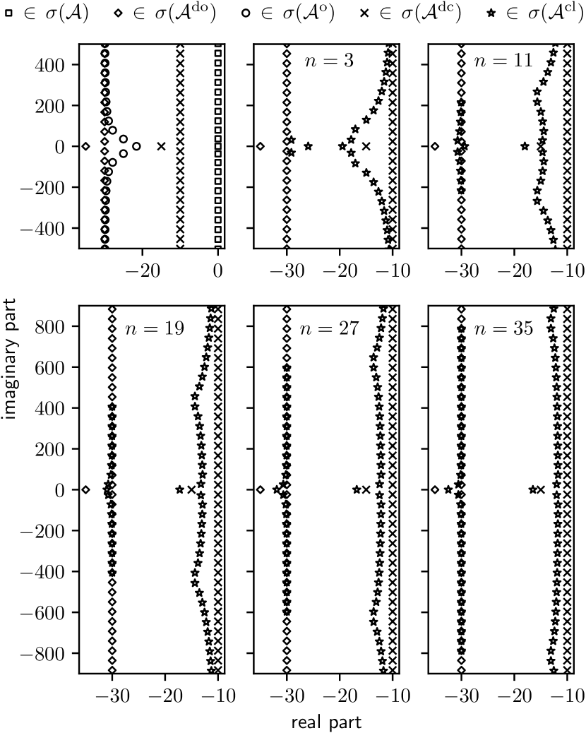
Figure 1: Different spectra for of the example system (7). Upper left: $\sigma(\mathcal{A})$, $\sigma(\mathcal{A}^{\text{\rm{dc}}})$, $\sigma(\mathcal{A}^{\text{\rm{do}}})$, $\sigma(\mathcal{A}^{\text{\rm{o}}})$. Other plots: $\sigma(\mathcal{A}^{\text{\rm{cl}}})$ for different approximation orders, together with desired closed-loop spectra $\sigma(\mathcal{A}^{\text{\rm{dc}}})$, $\sigma(\mathcal{A}^{\text{\rm{do}}})$.

5 Conclusion

An observer approximation scheme is proposed, which avoids possibly existing deviations in the output equation of standard modal approximation schemes. By combining this observer with late-lumping state feedback and late-lumping observer output injection, both described in (Riesmeier and Woittennek, 2022), an approximation scheme for FOSF is established, which can be applied to the considered class of BCS. For the closed-loop system operator, the RS property is proven. Therefore, the spectrum-determined growth condition holds. In contrast to previous results from (Curtain, 1984; Deutscher, 2013; Grüne and Meurer, 2022), the results not only hold for analytic systems but for rather general system operators satisfying the Assumptions 1 and 2. In particular, this includes certain hyperbolic systems.

References

- Bensoussan et al. (2007) Bensoussan, A., da Prato, G.D., Delfour, M.C., and Mitter, S.K. (2007). Representation and control of infinite dimensional systems. Systems Control: Foundations Applications. Birkhäuser, Boston, 2 edition.
- Curtain (1984) Curtain, R.F. (1984). Finite dimensional compensators for parabolic distributed systems with unbounded control and observation. SIAM J. Control Optim., 22, 255–276. 10.1137/0322018.
- Deutscher (2013) Deutscher, J. (2013). Finite-dimensional dual state feedback control of linear boundary control systems. International Journal of Control, 86, 41–53. 10.1080/00207179.2012.717723.
- Dunford and Schwartz (1971) Dunford, N. and Schwartz, J.T. (1971). Linear operators. Part 3: Spectral operators. Wiley. Wiley, New York.
- Fattorini (1968) Fattorini, H. (1968). Boundary control systems. SIAM J. Control, 6. 10.1137/0306025.
- Gehring and Kern (2018) Gehring, N. and Kern, R. (2018). Flatness-based tracking control for a pneumatic system with distributed parameters. In Proc. 9th Vienna Int. Conf. Math. Mod. (MATHMOD), 527–532.
- Grüne and Meurer (2022) Grüne, L. and Meurer, T. (2022). Finite-dimensional output stabilization for a class of linear distributed parameter systems — a small-gain approach. Systems & Control Letters, 164, 105237. https://doi.org/10.1016/j.sysconle.2022.105237.
- Guo and Zwart (2001) Guo, B.Z. and Zwart, H. (2001). Riesz spectral systems. Technical report, University Twente. Memorandum No. 1594.
- Kato (1995) Kato, T. (1995). Perturbation Theory for Linear Operators. Springer Verlag, Berlin Heidelberg, 2nd edition.
- Rebarber (1989) Rebarber, R. (1989). Spectral determination for a cantilever beam. IEEE Transactions on Automatic Control, 34(5), 502–510. 10.1109/9.24202.
- Riesmeier and Woittennek (2022) Riesmeier, M. and Woittennek, F. (2022). Late lumping of transformation-based feedback laws for boundary control systems. 10.48550/ARXIV.2211.01238. URL https://arxiv.org/abs/2211.01238.
- Tucsnak and Weiss (2009) Tucsnak, M. and Weiss, G. (2009). Observation and Control for Operator Semigroups. Birkhäuser Basel. 10.1007/978-3-7643-8994-9.
- Weiss (1994) Weiss, G. (1994). Transfer functions of regular linear systems. part i: Characterizations of regularity. Transactions of the American Mathematical Society, 342, 827–854. 10.2307/2154655.
- Xu and Sallet (1996) Xu, C.Z. and Sallet, G. (1996). On spectrum and Riesz basis assignment of infinite-dimensional linear systems by bounded linear feedbacks. SIAM Journal on Control and Optimization, 2, 1905 – 1910. 10.1109/CDC.1995.480622.