Learning to Play Trajectory Games
Against Opponents with Unknown Objectives

Abstract

Many autonomous agents, such as intelligent vehicles, are inherently required to interact with one another. Game theory provides a natural mathematical tool for robot motion planning in such interactive settings. However, tractable algorithms for such problems usually rely on a strong assumption, namely that the objectives of all players in the scene are known. To make such tools applicable for ego-centric planning with only local information, we propose an adaptive model-predictive game solver, which jointly infers other players’ objectives online and computes a corresponding generalized Nash equilibrium (GNE) strategy. The adaptivity of our approach is enabled by a differentiable trajectory game solver whose gradient signal is used for maximum likelihood estimation (MLE) of opponents’ objectives. This differentiability of our pipeline facilitates direct integration with other differentiable elements, such as neural networks (NNs). Furthermore, in contrast to existing solvers for cost inference in games, our method handles not only partial state observations but also general inequality constraints. In two simulated traffic scenarios, we find superior performance of our approach over both existing game-theoretic methods and non-game-theoretic model-predictive control (MPC) approaches. We also demonstrate our approach’s real-time planning capabilities and robustness in two hardware experiments.

I Introduction

Many robot planning problems, such as robot navigation in a crowded environment, involve rich interactions with other agents. Classic predict-then-plan frameworks neglect the fact that other agents in the scene are responsive to the ego-agent’s actions. This simplification can result in inefficient or even unsafe behavior [1]. Dynamic game theory explicitly models the interactions as coupled trajectory optimization problems from a multi-agent perspective. A noncooperative equilibrium solution of this game-theoretic model then provides strategies for all players that account for the strategic coupling of plans. Beyond that, general constraints between players, such as collision avoidance, can also be handled explicitly. All of these features render game-theoretic reasoning an attractive approach to interactive motion planning.

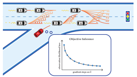
Figure 1: An ego-agent (red) merging onto a busy road populated by six surrounding vehicles whose preferences for travel velocity and lane are initially unknown. Our approach adapts the ego agent’s strategy by inferring opponents’ intention parameters $\tilde{\theta}$ from partial state observations.

In order to apply game-theoretic methods for interactive motion planning from an ego-centric rather than omniscient perspective, such methods must be capable of operating only based on local information. For instance, in driving scenarios as shown in Fig. 1, the red ego-vehicle may only have partial-state observations of the surrounding vehicles and incomplete knowledge of their objectives due to unknown preferences for travel velocity, target lane, or driving style. Since vanilla game-theoretic methods require an objective model of all players [2, 3], this requirement constitutes a key obstacle in applying such techniques for autonomous strategic decision-making.

To address this challenge, we introduce our main contribution: a model-predictive game solver, which adapts to unknown opponents’ objectives and solves for generalized Nash equilibrium (GNE)strategies. The adaptivity of our approach is enabled by a differentiable trajectory game solver whose gradient signal is used for MLE of opponents’ objectives.

We perform thorough experiments in simulation and on hardware to support the following three key claims: our solver (i) outperforms both game-theoretic and non-game-theoretic baselines in highly interactive scenarios, (ii) can be combined with other differentiable components such as NNs, and (iii) is fast and robust enough for real-time planning on a hardware platform.

II Related Work

To put our contribution into context, this section discusses four main bodies of related work. First, we discuss works on trajectory games which assume access to the objectives of all players in the scene. Then, we introduce works on inverse dynamic games that infer unknown objectives from data. Thereafter, we also relate our work to non-game-theoretic interaction-aware planning-techniques. Finally, we survey recent advances in differentiable optimization, which provide the underpinning for our proposed differentiable game solver.

II-A N-Player General-Sum Dynamic Games

Dynamic games are well-studied in the literature [4]. In robotics, a particular focus is on multi-player general-sum games in which players may have differing yet non-adversarial objectives, and states and inputs are continuous.

Various equilibrium concepts exist in dynamic games. The Stackelberg equilibrium concept [5] assumes a leader-follower hierarchy, while the Nash equilibrium problem (NEP) [2, 5] does not presume such a hierarchy. Within the scope of NEP, there exist open-loop NEPs [3] and feedback NEPs [2, 6]. We refer the readers to [4] for more details about the difference between the concepts. When shared constraints exist between players, such as collision avoidance constraints, one player’s feasible set may depend on other players’ decisions. In that case, the problem becomes a generalized Nash equilibrium problem (GNEP) [7]. In this work, we focus on GNEPs under an open-loop information pattern which we solve by converting to an equivalent Mixed Complementarity Problem (MCP) [8].

II-B Inverse Games

There are three main paradigms for solving inverse games: (i) Bayesian inference, (ii) minimization of Karush–Kuhn–Tucker (KKT) residuals, and (iii) equilibrium-constrained maximum-likelihood estimation. In type (i) methods, Le Cleac’h et al. [9] employ an Unscented Kalman Filter (UKF). This sigma-point sampling scheme drastically reduces the sampling complexity compared to vanilla particle filtering. However, a UKF is only applicable for uni-modal distributions, and extra care needs to be taken when uncertainty is multi-modal, e.g., due to multiple Nash equilibria. Type (ii) methods require full demonstration trajectories, i.e., including noise-free states and inputs, to cast the $N$-player inverse game as $N$ independent unconstrained optimization problems [10, 11]. However, they assume full constraint satisfaction at the demonstration and have limited scalability with noisy data [12]. The type (iii) methods use KKT conditions of an open-loop Nash equilibrium (OLNE) as constraints to formulate a constrained optimization problem [12]. This type of method finds the same solution as type (ii) methods in the noise-free cases but can additionally handle partial and noisy state observations. However, encoding the equilibrium constraints is challenging, as it typically yields a non-convex problem, even in relatively simple linear-quadratic game settings. This challenge is even more pronounced when considering inequality constraints of the observed game, as this results in complementarity constraints in the inverse problem.

Our solution approach also matches the observed trajectory data in an MLE framework. In contrast to all methods above, we do so by making a GNE solver differentiable. This approach yields two important benefits over existing methods: (i) general (coupled) inequality constraints can be handled explicitly, and (ii) the entire pipeline supports direct integration with other differentiable elements, such as NNs. This latter benefit is a key motivation for our approach that is not enabled by the formulations in [9] and [12].

Note that Geiger et al. [13] explore a similar differentiable pipeline for inference of game parameters. In contrast to their work, however, our method is not limited to the special class of potential games and applies to general GNEPs.

II-C Non-Game-Theoretic Interaction Models

Besides game-theoretic methods, two categories of interaction-aware decision-making techniques have been studied extensively in the context of collision avoidance and autonomous driving: (i) approaches that learn a navigation policy for the ego-agent directly without explicitly modeling the responses of others [14, 15, 16], and (ii) techniques that explicitly predict the opponents’ actions to inform the ego-agent’s decisions [17, 18, 19, 20, 21]. This latter category may be further split by the granularity of coupling between the ego-agent’s decision-making process and the predictions of others. In the simplest case, prediction depends only upon the current physical state of other agents [22]. More advanced interaction models condition the behavior prediction on additional information such as the interaction history [17], the ego-agent’s goal [19, 20], or even the ego-agent’s future trajectory [18, 21].

Our approach is most closely related to this latter body of work: by solving a trajectory game, our method captures the interdependence of future decisions of all agents; and by additionally inferring the objectives of others, predictions are conditioned on the interaction history. However, a key difference of our method is that it explicitly models others as rational agents unilaterally optimizing their own cost. This assumption provides additional structure and offers a level of interpretability of the inferred behavior.

II-D Differentiable Optimization

Our work is enabled by differentiating through a GNE solver. Several works have explored the idea of propagating gradient information through optimization algorithms [23, 24, 25], enabling more expressive neural architectures. However, these works focus on optimization problems and thus only apply to special cases of games, such as potential games studied by Geiger et al. [13]. By contrast, differentiating through a GNEP involves $N$ coupled optimization problems. We address this challenge in section IV-B.

III Preliminaries

This section introduces two key concepts underpinning our work: forward and inverse dynamic games. In forward games, the objectives of players are known, and the task is to find players’ strategies. By contrast, inverse games take (partial) observations of strategies as inputs to recover initially unknown objectives. In Section IV, we combine these two approaches into an adaptive solver that computes forward game solutions while estimating player objectives.

III-A General-Sum Trajectory Games

Consider an $N$-player discrete-time general-sum trajectory game with horizon of $T$. In this setting, each player $i$ has a control input $u_{t}^{i}\in\mathbb{R}^{m^{i}}$ which they may use to influence the their state $x_{t}^{i}\in\mathbb{R}^{n^{i}}$ at each discrete time $t\in[T]$. In this work, we assume that the evolution of each player’s state is characterized by an individual dynamical system $x_{t+1}^{i}=f^{i}(x_{t}^{i},u_{t}^{i})$. For brevity throughout the remainder of the paper, we shall use boldface to indicate aggregation over players and capitalization for aggregation over time, e.g., $\mathbf{x}_{t}:=(x_{t}^{1},\dots,x_{t}^{N})$, $U^{i}:=(u_{1}^{i},\dots,u_{T}^{i})$, $\mathbf{X}:=(\mathbf{x}_{1},\ldots,\mathbf{x}_{T})$. With a joint trajectory starting at a given initial state $\hat{\mathbf{x}}_{1}~{}:=~{}(\hat{x}_{1}^{1},\dots,\hat{x}_{1}^{N})$, each player seeks to find a control sequence $U^{i}$ to minimize their own cost function $J^{i}(\mathbf{X},U^{i};\theta^{i})$, which depends upon the joint state trajectory $\mathbf{X}$ as well as the player’s control input sequence $U^{i}$ and, additionally, takes in a parameter vector $\theta^{i}$. Each player must additionally consider private inequality constraints ${{}^{p}g^{i}}(X^{i},U^{i})~{}\geq~{}0$ as well as shared constraints ${}^{s}g(\mathbf{X},\mathbf{U})\geq 0$. This latter type of constraint is characterized by the fact that all players have a shared responsibility to satisfy it, with a common example being collision avoidance constraints between players. In summary, this noncooperative trajectory game can be cast as a tuple of $N$ coupled trajectory optimization problems:

$$\forall i\in[N]\left\{\begin{split}\mathop{\min}\limits_{X^{i},U^{i}}\hskip 5.69046pt&{J^{i}(\mathbf{X},U^{i};\theta^{i})}&\\ \text{s.t.}\hskip 5.69046pt&x_{t+1}^{i}=f^{i}(x_{t}^{i},u_{t}^{i}),\forall t\in[T-1]\\ &x_{1}^{i}=\hat{x}_{1}^{i}\\ &{}^{p}g^{i}(X^{i},U^{i})\geq 0&\\ &{}^{s}g(\mathbf{X},\mathbf{U})\geq 0.&\\ \end{split}\right.$$ (1)

Note that each player’s feasible set in this problem may depend upon the decision variables of others, which makes it a GNEP rather than a standard NEP [7].

A solution of this problem is a tuple of GNE strategies $\mathbf{U}^{*}:=(U^{1*},\dots,U^{N*})$ that satisfies the inequalities $J^{i}(\mathbf{X}^{*},U^{i*};\theta^{i})\leq J^{i}((X^{i},\mathbf{X}^{\neg i*}),U^{i};\theta^{i})$ for any feasible deviation $(X^{i},U^{i})$ of any player $i$, with $\mathbf{X}^{\neg i}$ denoting all but player $i$’s states. Since identifying a global GNE is generally intractable, we require these conditions only to hold locally. At a local GNE, then, no player has a unilateral incentive to deviate locally in feasible directions to reduce their cost.

Running example: We introduce a simple running example which we shall use throughout the presentation to concretize the key concepts. Consider a tracking game played between $N=2$ players. Let each agent’s dynamics be characterized by those of a planar double-integrator, where states $x^{i}_{t}=(p_{x,t}^{i},p_{y,t}^{i},v_{x,t}^{i},v_{y,t}^{i})$ are position and velocity, and control inputs $u^{i}_{t}=(a_{x,t}^{i},a_{y,t}^{i})$ are acceleration in horizontal and vertical axes in a Cartesian frame. We define the game’s state as the concatenation of the two players’ individual states $\mathbf{x}_{t}:=(x_{t}^{1},x_{t}^{2})$. Each player’s objective is characterized by an individual cost

$$J^{i}=\sum_{t=1}^{T-1}\|p_{t+1}^{i}-p^{i}_{\text{goal}}\|_{2}^{2}+0.1\|u_{t}^{i}\|_{2}^{2}\\ +50\max(0,d_{\min}-\|p_{t+1}^{i}-p_{t+1}^{-i}\|_{2})^{3},$$ (2)

where we set $p_{\text{goal}}^{1}=p_{t}^{2}$ so that player $1$, the tracking robot, is tasked to track player $2$, the target robot. Player $2$ has a fixed goal point $p_{\text{goal}}^{2}$. Both agents wish to get to their goal position efficiently while avoiding proximity beyond a minimal distance $d_{\text{min}}$. Players also have shared collision avoidance constraints ${{}^{s}g_{t+1}}(\mathbf{x}_{t+1},\mathbf{u}_{t+1})=\|p_{t+1}^{1}-p_{t+1}^{2}\|_{2}-d_{\min}\geq 0,\forall t\in[T-1]$ and private bounds on state and controls  ${}^{p}g^{i}(X^{i},U^{i})$. Agents need to negotiate and find an underlying equilibrium strategy in this noncooperative game, as no one wants to deviate from the direct path to their goal.

III-B Inverse Games

We now switch context to the inverse dynamic game setting. Let $\theta:=(\hat{\mathbf{x}}_{1},\theta^{2},...,\theta^{N})$ denote the aggregated tuple of parameters initially unknown to the ego-agent with index 1. Note that we explicitly infer the initial state of a game $\hat{\mathbf{x}}_{1}$ to account for the potential sensing noise and partial state observations. To model the inference task over these parameters, we assume that the ego-agent observes behavior originating from an unknown Nash game $\Gamma(\theta):=(\hat{\mathbf{x}}_{1},{{}^{s}g},\{f^{i},^{p}g^{i},J^{i}(\cdot;\theta^{i})\}_{i\in[N]})$, with objective functions and constraints parameterized by initially unknown values $\theta^{i}$ and $\hat{\mathbf{x}}_{1}$, respectively.

Similar to the existing method [12], we employ an MLE formulation to allow observations to be partial and noise-corrupted. In contrast to that method, however, we also allow for inequality constraints in the hidden game. That is, we propose to solve

$$\mathop{\max}\limits_{\theta,\mathbf{X},\mathbf{U}} {p(\mathbf{Y}\mid\mathbf{X},\mathbf{U})}$$ (3)

s.t. $$(\mathbf{X},\mathbf{U})\hskip 2.84544pt\text{is a}\hskip 2.84544pt\text{GNE}\hskip 2.84544pt\text{of}\hskip 2.84544pt\Gamma(\theta)$$

where $p(\mathbf{Y}\mid\mathbf{X},\mathbf{U})$ denotes the likelihood of observations $\mathbf{Y}:=(\mathbf{y}_{1},...,\mathbf{y}_{T})$ given the estimated game trajectory $(\mathbf{X},\mathbf{U})$ induced by parameters $\theta$. This formulation yields an mathematical program with equilibrium constraints (MPEC) [26], where the outer problem is an estimation problem while the inner problem involves solving a dynamic game. When the observed game includes inequality constraints, the resulting inverse problem necessarily contains complementarity constraints and only few tools are available to solve the resulting problem. In the next section, we show how to transform Eq. 3 into an unconstrained problem by making the inner game differentiable, which also enables combination with other differentiable components.

Running example: We assign the tracker (player 1) to be the ego-agent and parameterize the game with the goal position of the target robot $\theta^{2}=p_{\text{goal}}^{2}$. That is, the tracker does not know the target agent’s goal and tries to infer this parameter from position observations. To ensure that Eq. 3 remains tractable, the ego-agent maintains only a fixed-length buffer of observed opponent’s positions. Note that solving the inverse game requires solving games rather than optimal control problems at the inner level to account for the noncooperative nature of observed interactions, which is different from inverse optimal control (IOC) even in the $2$-player case. We employ a Gaussian observation model, which we represent with an equivalent negative log-likelihood objective $\|\mathbf{Y}-r(\mathbf{X},\mathbf{U})\|_{2}^{2}$ in Eq. 3, where $r(\mathbf{X},\mathbf{U})$ maps $(\mathbf{X},\mathbf{U})$ to the corresponding sequence of expected positions.

IV Adaptive Model-Predictive Game Play

We wish to solve the problem of model-predictive game play (MPGP) from an ego-centric perspective, i.e., without prior knowledge of other players’ objectives. To this end, we present an adaptive model-predictive game solver that combines the tools of Section III: first, we perform MLE of unknown objectives by solving an inverse game (Section III-B); then, we solve a forward game using this estimate to recover a strategic motion plan (Section III-A).

IV-A Forward Games as MCPs

We first discuss the conversion of the GNEP in Eq. 1 to an equivalent MCP. There are three main advantages of taking this view. First, there exists a wide range of off-the-shelf solvers for this problem class [27]. Furthermore, MCP solvers directly recover strategies for all players simultaneously. Finally, this formulation makes it easier to reason about derivatives of the solution w.r.t. to problem data. As we shall discuss in Section IV-C, this derivative information can be leveraged to solve the inverse game problem of Eq. 3.

In order to solve the GNEP presented in Eq. 1 we derive its first-order necessary conditions. We collect all equality constraints for player $i$ in Eq. 1 into a vector-valued function $h^{i}(X^{i},U^{i};\hat{x}^{i}_{1})$, introduce Lagrange multipliers $\mu^{i}$, ${{}^{p}\lambda^{i}}$ and ${{}^{s}\lambda}$ for constraints $h^{i}(X^{i},U^{i};\hat{x}^{i}_{1})$, ${{}^{p}g^{i}(X^{i},U^{i})}$, and ${{}^{s}g(\mathbf{X},\mathbf{U})}$ and write the Lagrangian for player $i$ as

$$\mathcal{L}^{i}(\mathbf{X},\mathbf{U},\mu^{i},{{}^{p}\lambda^{i}},{{}^{s}\lambda};\theta)=J^{i}(\mathbf{X},\mathbf{U};\theta^{i})$$ (4)

$$+\mu^{i\top}h^{i}(X^{i},U^{i};\hat{x}^{i}_{1})-{{}^{s}\lambda^{\top}}{{}^{s}g(\mathbf{X},\mathbf{U})}-{{}^{p}\lambda^{i\top}}{{}^{p}g^{i}(X^{i},U^{i})}.$$

Note that we share the multipliers associated with shared constraints between the players to encode equal constraint satisfaction responsibility [28]. Under mild regularity conditions, e.g., linear independence constraint qualification (LICQ), a solution of Eq. 1 must satisfy the following joint KKT conditions:

$$\forall i\in[N]\left\{\begin{aligned} \nabla_{(X^{i},U^{i})}\mathcal{L}^{i}(\mathbf{X},\mathbf{U},\mu^{i},{{}^{p}\lambda^{i}},{{}^{s}\lambda};\theta)=0\\ 0\leq{{}^{p}g^{i}(X^{i},U^{i})}\perp{{}^{p}\lambda^{i}}\geq 0\\ \end{aligned}\right.$$ (5)

$$h(\mathbf{X},\mathbf{U};\hat{\mathbf{x}}_{1})=0$$

$$0\leq{{}^{s}g(\mathbf{X},\mathbf{U})}\perp{{}^{s}\lambda}\geq 0,$$

where, for brevity, we denote by $h(\mathbf{X},\mathbf{U};\hat{\mathbf{x}}_{1})$ the aggregation of all equality constraints. If the second directional derivative of the Lagrangian is positive along all feasible directions at a solution of Eq. 5—a condition that can be checked a posteriori—this point is also a solution of the original game. In this work, we solve trajectory games by viewing their KKT conditions through the lens of MCPs [8, Section 1.4.2].

Definition 1

A Mixed Complementarity Problem (MCP)is defined by the following problem data: a function $F(z):\mathbb{R}^{d}\mapsto\mathbb{R}^{d}$, lower bounds $\ell_{j}\in\mathbb{R}\cup\{-\infty\}$ and upper bounds $u_{j}\in\mathbb{R}\cup\{\infty\}$, each for $j\in[d]$. The solution of an MCP is a vector $z^{*}\in\mathbb{R}^{n}$, such that for each element with index $j\in[d]$ one of the following equations holds:

$$z^{*}_{j}=\ell_{j},F_{j}(z^{*})\geq 0$$ (6a)

$$\ell_{j}<z^{*}_{j}<u_{j},F_{j}(z^{*})=0$$ (6b)

$$z^{*}_{j}=u_{j},F_{j}(z^{*})\leq 0.$$ (6c)

The parameterized KKT system of Eq. 5 can be expressed as a parameterized family of MCPs with decision variables corresponding to the primal and dual variables of Eq. 5,

$$z=\left[\mathbf{X}^{\top},\mathbf{U}^{\top},\boldsymbol{\mu}^{\top},{{}^{p}\lambda^{1\top}},\ldots,{{}^{p}\lambda^{N\top}},{{}^{s}\lambda^{\top}}\right]^{\top},$$

and problem data

$$F(z;\theta) =\begin{bmatrix}\nabla_{(X^{1},U^{1})}\mathcal{L}^{i}\\ \vdots\\ \nabla_{(X^{N},U^{N})}\mathcal{L}^{N}\\ h\\ {}^{p}g^{1}\\ \vdots\\ {}^{p}g^{N}\\ {}^{s}g\end{bmatrix}, \ell =\begin{bmatrix}-\infty\\ \vdots\\ -\infty\\ -\infty\\ 0\\ \vdots\\ 0\\ 0\end{bmatrix}, u =\begin{bmatrix}\infty\\ \vdots\\ \infty\\ \infty\\ \infty\\ \vdots\\ \infty\\ \infty\end{bmatrix},$$ (7)

where, by slight abuse of notation, we overload $F$ to be parametrized by $\theta$ via $\mathcal{L}^{i}$ and use $\infty$ to denote elements for which upper or lower bounds are dropped.

IV-B Differentiation of an MCP solver

An MCP solver may be viewed as a function, mapping problem data to a solution vector. Taking this perspective, for a parameterized family of MCPs as in Eq. 7, we wish to compute the function’s derivatives to answer the following question: How does the solution $z^{*}$ respond to local changes of the problem parameters $\theta$?

IV-B1 The Nominal Case

Let $\Psi(\theta):=(F(\cdot;\theta),\ell,u)$ denote an MCP parameterized by $\theta\in\mathbb{R}^{p}$ and let $z^{*}\in\mathbb{R}^{n}$ denote a solution of that MCP, which is implicitly a function of $\theta$. For this nominal case, we consider only solutions at which strict complementarity holds. We shall relax this assumption later. If $F$ is smooth, i.e., $F(\cdot;\theta),F(z^{*};\cdot)\in C^{1}$, we can recover the Jacobian matrix $\nabla_{\theta}z^{*}~{}=~{}\left(\frac{\partial z^{*}_{j}}{\partial\theta_{k}}\right)\in\mathbb{R}^{n\times p}$ by distinguishing two possible cases. For brevity, below, gradients are understood to be evaluated at $z^{*}$ and $\theta$.

Active bounds

Consider first the elements $z^{*}_{j}$ that are either at their lower or upper bound, i.e., $z^{*}_{j}$ satisfies Eq. 6a or Eq. 6c. Since strict complementarity holds at the solution, $F_{j}(z^{*};\theta)$ must be bounded away from zero with a finite margin. Hence, the smoothness of $F$ guarantees that a local perturbation of $\theta$ will retain the sign of $F_{j}(z^{*};\theta)$. As a result, $z^{*}_{j}$ remains at its bound and, locally, is identically zero. Let $\tilde{\mathcal{I}}:=\{k\in[n]\mid z_{k}^{*}=\ell_{k}\lor z_{k}^{*}=u_{k}\}$ denote the index set of all elements matching this condition and $\tilde{z}^{*}:=[z^{*}]_{\tilde{\mathcal{I}}}$ denote the solution vector reduced to that set. Trivially, then, the Jacobian of this vector vanishes, i.e., $\nabla_{\theta}\tilde{z}^{*}=0$.

Inactive bounds

The second case comprises elements that are strictly between the bounds, i.e., $z_{j}^{*}$ satisfying Eq. 6b. In this case, under mild assumptions on $F$, for any local perturbation of $\theta$ there exists a perturbed solution such that $F$ remains at its root. Therefore, the gradient $\nabla_{\theta}z_{j}^{*}$ for these elements is generally non-zero, and we can compute it via the implicit function theorem (IFT). Let $\bar{\mathcal{I}}:=\{k\in[n]\mid F_{k}(z^{*};\theta)=0,\ell_{k}<z^{*}_{k}<u_{k}\}$ be the index set of all elements satisfying case (b) and let

$$\bar{z}^{*} :=[z^{*}]_{\bar{\mathcal{I}}}, \bar{F}(z^{*},\theta) :=[F(z^{*};\theta)]_{\bar{\mathcal{I}}}$$ (8)

denote the solution vector and its complement reduced to said index set. By the IFT, the relationship between parameters $\theta$ and solution $z^{*}(\theta)$ is characterized by the stationarity of $\bar{F}$:

$$0=\nabla_{\theta}\left[\bar{F}(z^{*}(\theta),\theta)\right]=\\ \nabla_{\theta}\bar{F}+(\nabla_{\bar{z}^{*}}\bar{F})(\nabla_{\theta}\bar{z}^{*})+(\nabla_{\tilde{z}^{*}}\bar{F})\underbrace{(\nabla_{\theta}\tilde{z}^{*})}_{\equiv 0}$$ (9)

Note that, as per the discussion in case (a), the last term in this equation is identically zero. Hence, if the Jacobian $\nabla_{\bar{z}^{*}}\bar{F}$ is invertible, we recover the derivatives as the unique solution of the above system of equations,

$$\nabla_{\theta}\bar{z}^{*}=-\left(\nabla_{\bar{z}^{*}}\bar{F}\right)^{-1}(\nabla_{\theta}\bar{F}).$$ (10)

Note that Eq. 9 may not always have a unique solution, in which case Eq. 10 cannot be evaluated. We discuss practical considerations for this special case below.

IV-B2 Remarks on Special Cases and Practical Realization

The above derivation of gradients for the nominal case involves several assumptions on the structure of the problem. We discuss considerations to improve numerical robustness for practical realization of this approach below. We note that both special cases discussed hereafter are rare in practice. In fact, across 100 simulations of the running example with varying initial states and objectives, neither of them occurred.

Weak Complementarity

The nominal case discussed above assumes strict complementarity at the solution. If this assumption does not hold, the derivative of the MCP is not defined. Nevertheless, we can still compute subderivatives at $\theta$. Let the set of all indices for which this condition holds be denoted by $\hat{\mathcal{I}}:=\{k\in[n]\mid F_{k}(z^{*};\theta)=0\land z_{k}^{*}\in\{\ell_{k},u_{k}\}\}$. Then by selecting a subset of $\hat{\mathcal{I}}$ and including it in $\bar{\mathcal{I}}$ for evaluation of Eq. 10, we recover a subderivative.

Invertibility

The evaluation Eq. 10 requires invertibility of $\nabla_{\bar{z}^{*}}\bar{F}$. To this end, we compute the least-squares solution of Eq. 9 rather than explicitly inverting $\nabla_{\bar{z}}\bar{F}$.

IV-C Model-Predictive Game Play with Gradient Descent

Finally, we present our pipeline for adaptive game-play against opponents with unknown objectives. Our adaptive MPGP scheme is summarized in Algorithm 1. At each time step, we first update our estimate of the parameters by approximating the inverse game in Eq. 3 via gradient descent. To obtain an unconstrained optimization problem, we substitute the constraints in Eq. 3 with our differentiable game solver. Following the discussion of Eq. 7, we denote by $z^{*}(\theta)$ the solution of the MCP formulation of the game parameterized by $\theta$. Furthermore, by slight abuse of notation, we overload $\mathbf{X}(z^{*}),\mathbf{U}(z^{*})$ to denote functions that extract the state and input vectors from $z^{*}$. Then, the inverse game of Eq. 3 can be written as unconstrained optimization,

$$\mathop{\max}\limits_{\theta} {p(\mathbf{Y}\mid\mathbf{X}(z^{*}(\theta)),\mathbf{U}(z^{*}(\theta)))}.$$ (11)

Online, we approximate solutions of this problem by taking gradient descent steps on the negative logarithm of this objective, with gradients computed by chain rule,

$$\begin{split}\nabla_{\theta}\left[p(\mathbf{Y}\mid\mathbf{X}(z^{*}(\theta)),\mathbf{U}(z^{*}(\theta))\right]=\\ (\nabla_{\mathbf{X}}p)(\nabla_{z^{*}}\mathbf{X})(\nabla_{\theta}z^{*})+(\nabla_{\mathbf{U}}p)(\nabla_{z^{*}}\mathbf{U})(\nabla_{\theta}z^{*}).\end{split}$$ (12)

Here, the only non-trivial term is $\nabla_{\theta}z^{*}$, whose computation we discussed in Section IV-B. To reduce the computational cost, we warm-start using the estimate of the previous time step and terminate early if a maximum number of steps is reached. Then, we solve a forward game parametrized by the estimated $\tilde{\theta}$ to compute control commands. We execute the first control input for the ego agent and repeat the procedure.

Hyper-parameters: stopping tolerance: $\mathrm{stop\_tol}$, learning rate: $\mathrm{lr}$

Input: initial $\tilde{\theta}$, current observation buffer $\mathbf{Y}$, new observation $\mathbf{y}$

$\mathbf{Y}\leftarrow$ updateBuffer$(\mathbf{Y},\mathbf{y})$

/* inverse game approximation */

while $\mathrm{not~{}stop\_tol~{}and~{}not~{}max\_steps\_reached}$ do

       $(z^{*},\nabla_{\theta}z^{*})\leftarrow\operatorname{solveDiffMCP}(\tilde{\theta})$ $\triangleright$ sec. IV-B

       $\nabla_{\theta}p\leftarrow\operatorname{composeGradient}(z^{*},\nabla_{\theta}z^{*},\mathbf{Y})$ $\triangleright$ eq. (12)

       $\tilde{\theta}\leftarrow\tilde{\theta}-\nabla_{\theta}p\cdot\mathrm{lr}$

      

end while

$z^{*}\leftarrow\operatorname{solveMCP}(\tilde{\theta})$ $\triangleright$ forward game, eq. (7)

$\operatorname{applyFirstEgoInput}(z^{*})$

return $\tilde{\theta},\mathbf{Y}$

Algorithm 1 Adaptive MPGP

V Experiments

To evaluate our method, we compare against two baselines in Monte Carlo studies of simulated interaction. Beyond these quantitative results, we showcase our method deployed on Jackal ground robots in two hardware experiments.

The experiments below are designed to support the key claims that our method (i) outperforms both game-theoretic and non-game-theoretic baselines in highly interactive scenarios, (ii) can be combined with other differentiable components such as NNs, and (iii) is sufficiently fast and robust for real-time planning on a hardware platform. A supplementary video of qualitative results can be found at https://xinjie-liu.github.io/projects/game. Upon publication of this manuscript, the code for our method and experiments will be available at the same link.

V-A Experiment Setup

V-A1 Scenarios

We evaluate our method in two scenarios.

2-player running example

To test the inference accuracy and convergence of our method in an intuitive setting, we first consider the 2-player running example. For evaluation in simulation, we sample the opponent’s intent—i.e., their unknown goal position in Eq. 2— uniformly from the environment. Partial observations comprise the position of each agent.

Ramp merging

To demonstrate the scalability of our approach and support the claim that our solver outperforms the baselines in highly interactive settings, we also test our method on a ramp merging scenario with varying numbers of players. This experiment is inspired by the setup used in [3] and is schematically visualized in Fig. 1. We model each player’s dynamics by a discrete-time kinematic bicycle with the state comprising position, velocity and orientation, i.e., $x_{t}^{i}=(p_{x,t}^{i},p_{y,t}^{i},v_{t}^{i},\psi_{t}^{i})$, and controls comprising acceleration and steering angle, i.e., $u_{t}^{i}=(a_{t}^{i},\phi)$. We capture their individual behavior by a cost function that penalizes deviation from a reference travel velocity and target lane; i.e., $\theta^{i}=(v_{\textrm{ref}}^{i},p_{\textrm{y,lane}}^{i})$. We add constraints for lane boundaries, for limits on speed, steering, and acceleration, for the traffic light, and for collision avoidance. To encourage rich interaction in simulation, we sample each agent’s initial state by sampling their speed and longitudinal positions uniformly at random from the intervals from zero to maximum velocity $v_{\mathrm{max}}$ and four times the vehicle length ${l_{\mathrm{car}}}$, respectively. The ego-agent always starts on the ramp and all agents are initially aligned with their current lane. Finally, we sample each opponent’s intent from the uniform distribution over the two lane centers and the target speed interval $[0.4v_{\mathrm{max}},v_{\mathrm{max}}]$. Partial observations comprise the position and orientation of each agent.

V-A2 Baselines

We consider the following three baselines.

KKT-Constrained Solver

In contrast to our method, the solver by Peters et al. [12] has no support for either private or shared inequality constraints. Consequently, this baseline can be viewed as solving a simplified version of the problem in Eq. 3 where the inequality constraints associated with the inner-level GNEP are dropped. Nonetheless, we still use a cubic penalty term as in Eq. 2 to encode soft collision avoidance. Furthermore, for fair comparison, we only use the baseline to estimate the objectives but compute control commands from a GNEP considering all constraints.

MPC with Constant-Velocity Predictions

This baseline assumes that opponents move with constant velocity as observed at the latest time step. We use this baseline as a representative method for predictive planning approaches that do not explicitly model interaction.

Heuristic Estimation MPGP

To highlight the importance of online intent inference, for the ramp merging evaluation, we also compare against a game-theoretic baseline that assumes a fixed intent for all opponents. This fixed intent is recovered by taking each agent’s initial lane and velocity as a heuristic preference estimate.

To ensure a fair comparison, we use the same MCP backend [29] to solve all GNEP s and optimization problems with a default convergence tolerance of $1e^{-6}$. Furthermore, all planners utilize the same planning horizon and history buffer size of $10$ time steps with a time-discretization of $0.1\text{\,}\mathrm{s}$. For the iterative MLE solve procedure in the $2$-player running example and the ramp merging scenario, we employ a learning rate of $2e^{-2}$ for objective parameters and $1e^{-3}$ for initial states. We terminate maximum likelihood estimation iteration when the norm of the parameter update step is smaller than $1e^{-4}$, or after a maximum of $30$ steps. Finally, opponent behavior is generated by solving a separate ground-truth game whose parameters are hidden from the ego-agent.

V-B Simulation Results

To compare the performance of our method to the baselines described in Section V-A2, we conduct a Monte Carlo study for the two scenarios described in Section V-A1.

V-B1 $2$-Player Running Example

Figure 2: Monte Carlo study for the $2$-player tracking game for $100$ trials. Solid lines and ribbons in (a) and (b) indicate the mean and standard error of the mean. Cost distributions in (c) are normalized by subtracting ground truth costs.

Figure 2 summarizes the results for the 2-player running example. For this evaluation, we filter out any runs for which a solver resulted in a collision. For our solver, the KKT-constrained baseline, and the MPC baseline this amounts to $2,2$ and $13$ out of $100$ episodes, respectively.

Figures 2(a-b) show the prediction error of the goal position and opponent’s trajectory, each of which is measured by $\ell^{2}$-norm. Since the MPC baseline does not explicitly reason about costs of others, we do not report parameter inference error for it in Fig. 2a. As evident from this visualization, both game-theoretic methods give relatively accurate parameter estimates and trajectory predictions. Among these methods, our solver converges more quickly and consistently yields a lower error. By contrast, MPC gives inferior prediction performance with reduced errors only in trivial cases, when the target robot is already at the goal. Figure 2c shows the distribution of costs incurred by the ego-agent for the same set of experiments. Again, game-theoretic methods yield better performance and our method outperforms the baselines with more consistent and robust behaviors, indicated by fewer outliers and lower variance in performance.

V-B2 Ramp Merging

Set.	Method	Ego cost	Opp. cost	Coll.	Inf.	Traj. err. [m]	Param. err.	Time [s]
3 player	Ours	0.64 $\pm$ 0.36	0.06 $\pm$ 0.03	0	0	1.29 $\pm$ 0.05	0.41 $\pm$ 0.03	0.081 $\pm$ 0.002
	KKT-con	1.85 $\pm$ 1.21	0.05 $\pm$ 0.02	0	1	1.32 $\pm$ 0.06	2.39 $\pm$ 0.11	0.060 $\pm$ 0.002
	Heuristic	6.73 $\pm$ 2.40	0.09 $\pm$ 0.07	0	11	7.89 $\pm$ 0.26	3.96 $\pm$ 0.13	0.008 $\pm$ 0.001
	MPC	1.50 $\pm$ 0.45	0.33 $\pm$ 0.07	28	218	2.40 $\pm$ 0.11	n/a	0.009 $\pm$ 0.002
5 player	Ours	0.56 $\pm$ 0.43	0.16 $\pm$ 0.06	0	2	1.66 $\pm$ 0.07	0.47 $\pm$ 0.03	0.29 $\pm$ 0.02
	KKT-con	0.07 $\pm$ 0.32	0.06 $\pm$ 0.02	1	4	1.70 $\pm$ 0.06	2.15 $\pm$ 0.06	0.28 $\pm$ 0.02
	Heuristic	2.06 $\pm$ 0.44	0.35 $\pm$ 0.10	5	25	8.05 $\pm$ 0.19	2.91 $\pm$ 0.07	0.015 $\pm$ 0.001
	MPC	5.73 $\pm$ 2.91	0.42 $\pm$ 0.13	44	552	2.87 $\pm$ 0.13	n/a	0.014 $\pm$ 0.002
7 player	Ours	1.60 $\pm$ 1.19	0.06 $\pm$ 0.02	1	1	1.89 $\pm$ 0.05	0.46 $\pm$ 0.02	0.68 $\pm$ 0.02
	KKT-con	3.11 $\pm$ 1.72	0.09 $\pm$ 0.04	7	22	2.01 $\pm$ 0.06	1.93 $\pm$ 0.03	0.63 $\pm$ 0.06
	Heuristic	6.60 $\pm$ 1.67	0.27 $\pm$ 0.06	8	8	8.18 $\pm$ 0.15	2.44 $\pm$ 0.05	0.031 $\pm$ 0.002
	MPC	8.41 $\pm$ 1.45	0.59 $\pm$ 0.09	43	848	3.07 $\pm$ 0.08	n/a	0.0274 $\pm$ 0.004

TABLE I: Monte Carlo study for the ramp merging scenario depicted in Fig. 1 with $100$ trials for settings with 3, 5, and 7 players. Except for collision and infeasible solve times, all metrics are reported by mean and standard error of the mean.

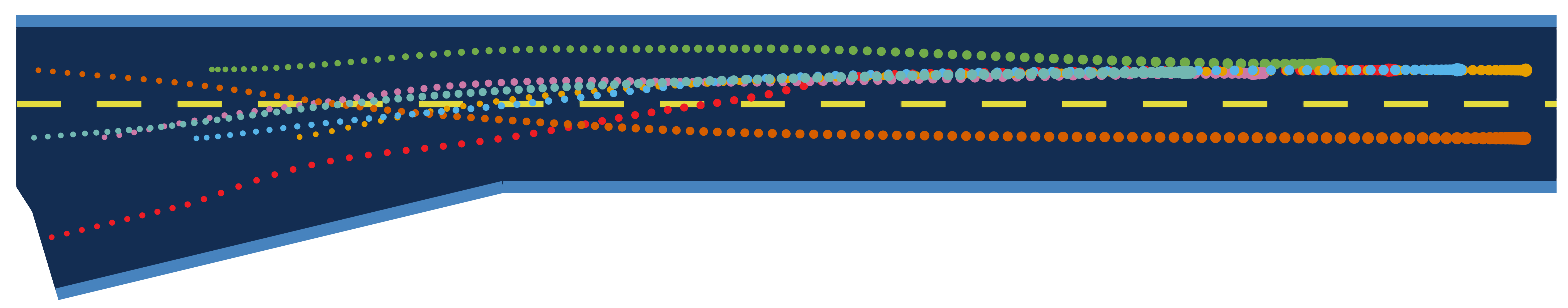
(a) Qualitative performance.

Ego cost	Opp. cost	Coll.	Inf.	Traj. err. [m]	Param. err.	Time [2]
2.19 $\pm$ 1.21	0.17 $\pm$ 0.07	3	5	2.34 $\pm$ 0.08	0.91 $\pm$ 0.08	0.274 $\pm$ 0.01

(b) Quantitative performance.

Figure 3: Performance of our solver in combination with an NN for 100 trials of the 7-player ramp merging scenario.

Table I summarizes the results of for the simulated ramp-merging scenario for 3, 5, and 7 players.

Task Performance

To quantify the task performance, we report costs as an indicator for interaction efficiency, the number of collisions as a measure of safety, number of infeasible solves as an indicator of robustness, and trajectory and parameter error as a measure of inference accuracy. On a high level, we observe that the game-theoretic methods generally outperform the other baselines; especially for the settings with higher traffic density. While MPC achieves high efficiency (ego-cost) in the 3-player case, it collides significantly more often than the other methods across all settings. Among the game-theoretic approaches, we observe that online inference of opponent intents—as performed by our method and the KKT-constrained baseline—yields better performance than a game that uses a heuristic estimate of the intents. Within the inference-based game solvers, a Manning-Whitney U-test reveals that, across all settings, both methods achieve an ego-cost that is significantly lower than all other baselines but not significantly higher than solving the game with ground truth opponent intents. Despite this tie in terms of interaction efficiency, we observe a statistically significant improvement of our method over the KKT-constrained baseline in terms of safety: in the highly interactive 7-player case, the KKT-constrained baseline collides seven times more often than our method. This advantage is enabled by our method’s ability to model inequality constraints within the inverse game.

Computation Time

We also measure the computation time of each approach. The inference-based game solvers have generally a higher runtime than the remaining methods due to the added complexity. Within the inference methods, our method is only marginally slower than the KKT-constrained baseline, despite solving a more complex problem that includes inequality constraints. The average number of MLE updates for our method was $11.0$, $19.2$, and $22.7$ for the 3, 5, and 7-player setting, respectively. While our current implementation achieves real-time planning rates only for up to three players, we note that additional optimizations may further reduce the runtime of our approach. Among such optimizations are low-level changes such as sharing memory between MLE updates as well as algorithmic changes to perform intent inference asynchronously at an update rate lower than the control rate. We briefly explore another algorithmic optimization in the next section.

V-B3 Combination with an NN

To support the claim that our method can be combined with other differentiable modules, we demonstrate the integration with an NN. For this proof of concept, we use a two-layer feed-forward NN, which takes the buffer of recent partial state observations as input and predicts other players’ objectives. Training of this module is enabled by propagating the gradient of the observation likelihood loss of Eq. 11 through the differentiable game solver to the parameters of the NN. Online, we use the network’s prediction as an initial guess to reduce the number gradient steps. As summarized in Fig. 3, this combination reduces the computation time by more than 60% while incurring only a marginal loss in performance.

V-C Hardware Experiments

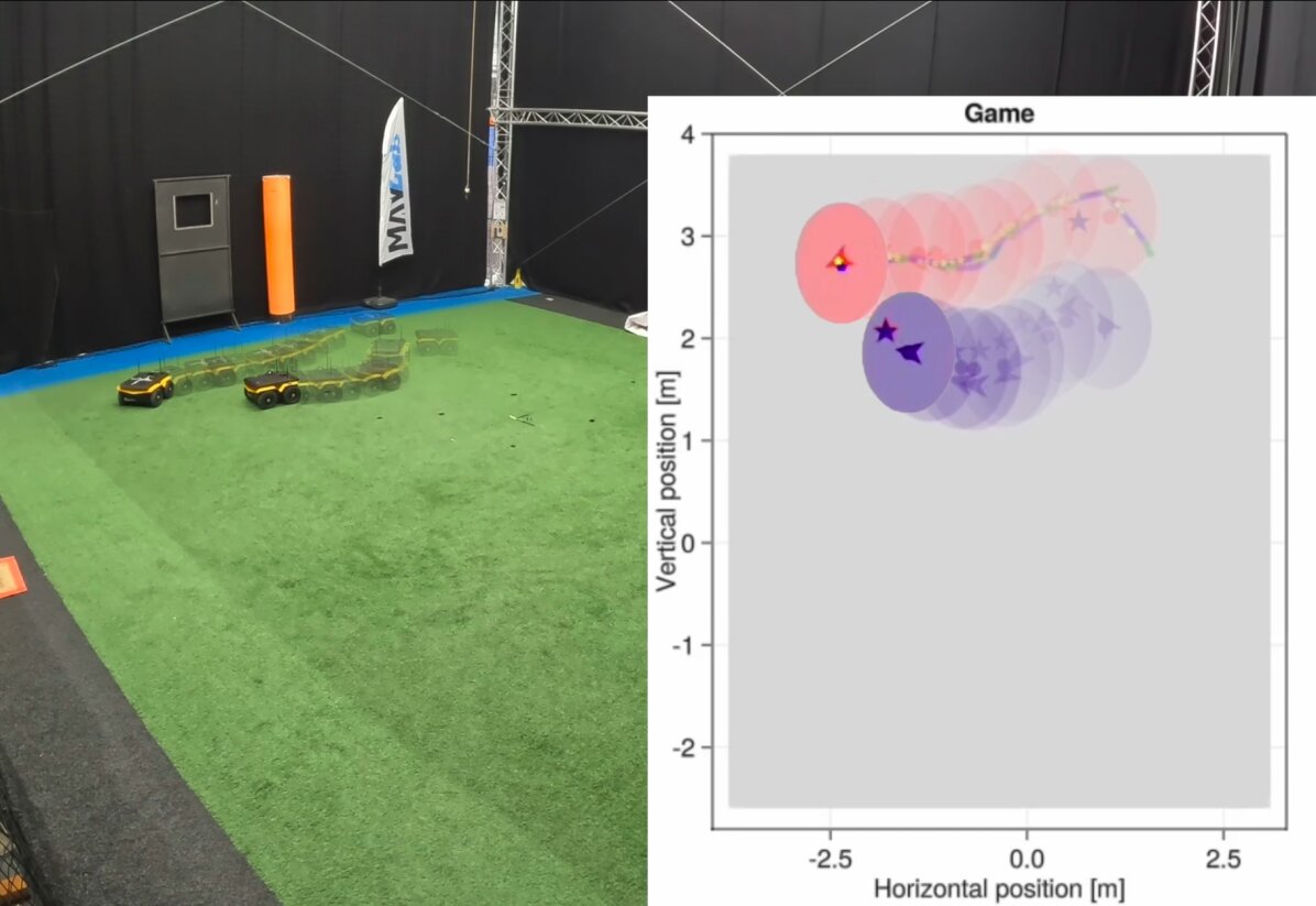
(a)

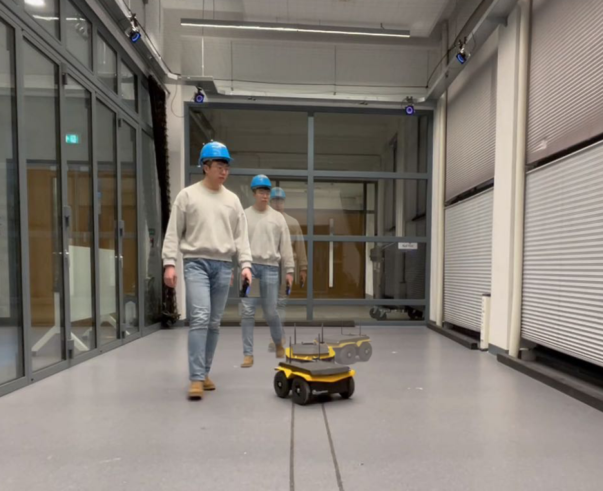
(b)

Figure 4: Time lapse of the running-example in which a Jackal tracks (a) another Jackal and (b) a human. Overlaid in (a) are the position of target robot (red) its true goal (red star), the tracker (blue), and its goal estimate (blue star).

To support the claim that our method is sufficiently fast and robust for hardware deployment, we demonstrate the tracking game in the running example in Section III-A with a Jackal ground robot tracking (i) another Jackal robot (Fig. 4(a)) and (ii) a human player (Fig. 4(b)), each with initially unknown goals. Plans are computed online on a mobile i$7$ CPU. We generate plans using the point mass dynamics with a velocity constraint of $0.8\text{\,}\mathrm{m}\text{\,}{\mathrm{s}}^{-1}$ and realize low-level control via the feedback controller of [30]. A video of these hardware demonstrations is included in the supplementary material. In both experiments, we observe that our adaptive MPGP planner enables the robot to infer the unknown goal position to track the target while avoiding collisions. The average computation time in both experiments was $0.035\text{\,}\mathrm{s}$.

VI Conclusion

In this paper, we presented a model-predictive game solver that adapts strategic motion plans to initially unknown opponents’ objectives. The adaptivity of our approach is enabled by a differentiable trajectory game solver whose gradient signal is used for MLE of unknown game parameters. As a result, our adaptive MPGP planner allows for safe and efficient interaction with other strategic agents without assuming prior knowledge of their objectives or observations of full states. We evaluated our method in two simulated interaction scenarios and demonstrated superior performance over a state-of-the-art game-theoretic planner and a non-interactive MPC baseline. Beyond that, we demonstrated the real-time planning capability and robustness of our approach in two hardware experiments.

In this work, we have limited inference to parameters that appear in the objectives of other players. Since the derivation of the gradient in Section IV-B can also handle other parameterizations of $F$—so long as they are smooth—future work may extend this framework to infer additional parameters of constraints or aspects of the observation model. Furthermore, encouraged by the improved scalability when combining our method with learning modules such as NNs, we seek to extend this learning pipeline in the future. One such extension would be to operate directly on raw sensor data, such as images, to exploit additional visual cues for intent inference. Another extension is to move beyond MLE-based point estimates to inference of potentially multi-modal distributions over opponent intents, which may be achieved by embedding our differentiable method within a variational autoencoder. Finally, our framework could be tested on large-scale datasets of real autonomous-driving behavior.

References

- [1] P. Trautman and A. Krause, “Unfreezing the robot: Navigation in dense, interacting crowds,” in Proc. of the IEEE/RSJ Intl. Conf. on Intelligent Robots and Systems (IROS), 2010.
- [2] D. Fridovich-Keil, E. Ratner, L. Peters, A. D. Dragan, and C. J. Tomlin, “Efficient iterative linear-quadratic approximations for nonlinear multi-player general-sum differential games,” in Proc. of the IEEE Intl. Conf. on Robotics & Automation (ICRA), 2020.
- [3] L. Cleac’h, M. Schwager, and Z. Manchester, “ALGAMES: A fast augmented lagrangian solver for constrained dynamic games,” Autonomous Robots, vol. 46, no. 1, pp. 201–215, 2022.
- [4] T. Başar and G. J. Olsder, Dynamic Noncooperative Game Theory, 2nd ed. Society for Industrial and Applied Mathematics (SIAM), 1999.
- [5] A. Liniger and J. Lygeros, “A noncooperative game approach to autonomous racing,” IEEE Trans. on Control Systems Technology (TCST), vol. 28, no. 3, pp. 884–897, 2019.
- [6] F. Laine, D. Fridovich-Keil, C.-Y. Chiu, and C. Tomlin, “The computation of approximate generalized feedback Nash equilibria,” arXiv preprint arXiv:2101.02900, 2021.
- [7] F. Facchinei and C. Kanzow, “Generalized Nash equilibrium problems,” Annals of Operations Research, vol. 175, no. 1, pp. 177–211, 2010.
- [8] F. Facchinei and J.-S. Pang, Finite-Dimensional Variational Inequalities and Complementarity Problems. Springer Verlag, 2003.
- [9] S. Le Cleac’h, M. Schwager, and Z. Manchester, “LUCIDGames: Online unscented inverse dynamic games for adaptive trajectory prediction and planning,” IEEE Robotics and Automation Letters (RA-L), vol. 6, no. 3, pp. 5485–5492, 2021.
- [10] C. Awasthi and A. Lamperski, “Inverse differential games with mixed inequality constraints,” in Proc. of the IEEE American Control Conference (ACC), 2020.
- [11] S. Rothfuß, J. Inga, F. Köpf, M. Flad, and S. Hohmann, “Inverse optimal control for identification in non-cooperative differential games,” IFAC-PapersOnLine, vol. 50, no. 1, pp. 14 909–14 915, 2017.
- [12] L. Peters, D. Fridovich-Keil, V. R. Royo, C. J. Tomlin, and C. Stachniss, “Inferring objectives in continuous dynamic games from noise-corrupted partial state observations,” in Proc. of Robotics: Science and Systems (RSS), 2021.
- [13] P. Geiger and C.-N. Straehle, “Learning game-theoretic models of multiagent trajectories using implicit layers,” in Proc. of the Conference on Advancements of Artificial Intelligence (AAAI), vol. 35, no. 6, 2021.
- [14] M. Everett, Y. F. Chen, and J. P. How, “Motion planning among dynamic, decision-making agents with deep reinforcement learning,” in Proc. of the IEEE/RSJ Intl. Conf. on Intelligent Robots and Systems (IROS), 2018.
- [15] B. Brito, M. Everett, J. P. How, and J. Alonso-Mora, “Where to go next: Learning a subgoal recommendation policy for navigation in dynamic environments,” IEEE Robotics and Automation Letters (RA-L), vol. 6, no. 3, pp. 4616–4623, 2021.
- [16] V. Tolani, S. Bansal, A. Faust, and C. Tomlin, “Visual navigation among humans with optimal control as a supervisor,” IEEE Robotics and Automation Letters (RA-L), vol. 6, no. 2, pp. 2288–2295, 2021.
- [17] H. Kretzschmar, M. Spies, C. Sprunk, and W. Burgard, “Socially compliant mobile robot navigation via inverse reinforcement learning,” Intl. Journal of Robotics Research (IJRR), vol. 35, no. 11, pp. 1289–1307, 2016.
- [18] E. Schmerling, K. Leung, W. Vollprecht, and M. Pavone, “Multimodal probabilistic model-based planning for human-robot interaction,” in Proc. of the IEEE Intl. Conf. on Robotics & Automation (ICRA), 2018.
- [19] N. Rhinehart, R. McAllister, K. Kitani, and S. Levine, “Precog: Prediction conditioned on goals in visual multi-agent settings,” in Proc. of the IEEE/CVF Intl. Conf. on Computer Vision (ICCV), 2019.
- [20] J. Roh, C. Mavrogiannis, R. Madan, D. Fox, and S. Srinivasa, “Multimodal trajectory prediction via topological invariance for navigation at uncontrolled intersections,” in Proc. of the Conf. on Robot Learning (CoRL), 2021.
- [21] M. Sun, F. Baldini, P. Trautman, and T. Murphey, “Move beyond trajectories: Distribution space coupling for crowd navigation,” Proc. of Robotics: Science and Systems (RSS), 2021.
- [22] C. Schöller, V. Aravantinos, F. Lay, and A. Knoll, “What the constant velocity model can teach us about pedestrian motion prediction,” IEEE Robotics and Automation Letters (RA-L), vol. 5, no. 2, pp. 1696–1703, 2020.
- [23] D. Ralph and S. Dempe, “Directional derivatives of the solution of a parametric nonlinear program,” Mathematical Programming, vol. 70, no. 1, pp. 159–172, 1995.
- [24] B. Amos and J. Z. Kolter, “Optnet: Differentiable optimization as a layer in neural networks,” in Proc. of the Int. Conf. on Machine Learning (ICML). PMLR, 2017.
- [25] A. Agrawal, B. Amos, S. Barratt, S. Boyd, S. Diamond, and J. Z. Kolter, “Differentiable convex optimization layers,” Proc. of the Advances in Neural Information Processing Systems (NIPS), 2019.
- [26] Z.-Q. Luo, J.-S. Pang, and D. Ralph, Mathematical programs with equilibrium constraints. Cambridge University Press, 1996.
- [27] S. C. Billups, S. P. Dirkse, and M. C. Ferris, “A comparison of large scale mixed complementarity problem solvers,” Computational Optimization and Applications, vol. 7, no. 1, pp. 3–25, 1997.
- [28] A. A. Kulkarni and U. V. Shanbhag, “On the variational equilibrium as a refinement of the generalized nash equilibrium,” Automatica, vol. 48, no. 1, pp. 45–55, 2012.
- [29] S. P. Dirkse and M. C. Ferris, “The PATH solver: A nommonotone stabilization scheme for mixed complementarity problems,” Optimization methods and software, vol. 5, no. 2, pp. 123–156, 1995.
- [30] Y. Kanayama, Y. Kimura, F. Miyazaki, and T. Noguchi, “A stable tracking control method for an autonomous mobile robot,” in Proc. of the IEEE Intl. Conf. on Robotics & Automation (ICRA), 1990.