Impact of NOMA on Age of Information:
A Grant-Free Transmission Perspective

Abstract

The aim of this paper is to characterize the impact of non-orthogonal multiple access (NOMA) on the age of information (AoI) of grant-free transmission. In particular, a low-complexity form of NOMA, termed NOMA-assisted random access, is applied to grant-free transmission in order to illustrate the two benefits of NOMA for AoI reduction, namely increasing channel access and reducing user collisions. Closed-form analytical expressions for the AoI achieved by NOMA assisted grant-free transmission are obtained, and asymptotic studies are carried out to demonstrate that the use of the simplest form of NOMA is already sufficient to reduce the AoI of orthogonal multiple access (OMA) by more than $40\%$. In addition, the developed analytical expressions are also shown to be useful for optimizing the users’ transmission attempt probabilities, which are key parameters for grant-free transmission.

I Introduction

Grant-free transmission is an important enabling technique to support the sixth-generation (6G) services, including ultra massive machine type communications (umMTC) and enhanced ultra-reliable low latency communications (euRLLC) [1, 2]. Unlike conventional grant-based transmission, grant-free transmission enables users to avoid multi-step signalling and directly transmit data signals together with access control information, which can reduce the system overhead significantly, particularly for scenarios with massive users requiring short-package transmission. Grant-free transmission can be realized by applying the random access protocols developed for conventional computer networks, such as ALOHA random access [3, 4]. Alternatively, massive multi-input multi-output (MIMO) can also be applied to support grant-free transmission by using the excessive spatial degrees of freedom offered by massive MIMO [5, 6, 7].

Recently, the application of non-orthogonal multiple access (NOMA) to grant-free transmission has received significant attention due to the following two reasons. First, the NOMA principle is highly compatible, and the use of NOMA can significantly improve the reliability and spectral efficiency of random access and massive MIMO based grant-free protocols [8, 9, 10, 11]. Second, more importantly, the use of NOMA alone is sufficient to support grant-free transmission. For example, NOMA-based grant-free transmission has been proposed in [12], where a Bayesian learning based scheme has been designed to ensure successful multi-user detection, even if the number of active grant-free users is unknown. The principle of NOMA can also be used to develop so-called semi-grant-free transmission protocols, where the bandwidth resources which would be solely occupied by grant-based users are released for supporting multiple grant-free users in a distributed manner [13]. In addition, NOMA-based grant-free transmission has also been shown to be robust and efficient in various communication scenarios, such as satellite communication networks, secure Internet of Things (IoT), intelligent reflecting surface (IRS) networks, marine communication systems, etc., see [14, 15, 16, 17].

The aim of this paper is to characterize the impact of NOMA on the performance of grant-free transmission with respect to a recently developed new performance metric, termed the age of information (AoI) [18, 19, 20]. In particular, the AoI describes the freshness of data updates collected in the network, and is an important metric to measure the success of the 6G services, including umMTC and euRLLC. We note that most existing works have focused on the impact of NOMA on grant-based networks [21, 22, 23, 24, 25]. For example, for two-user grant-based networks, the capability of NOMA to reduce the AoI has been shown to be related to the spectral efficiency gain of NOMA over orthogonal multiple access (OMA) [26]. To the authors’ best knowledge, there is only a single existing work which applied NOMA to reduce the AoI of grant-free transmission [27], where the strong assumption that the base station estimates all users’ channel state information (CSI) was made.

In this paper, the impact of NOMA on the AoI of grant-free transmission is investigated from the perspective of performance analysis, which is different from the existing work focusing on resource allocation [28]. In particular, a low-complexity form of NOMA, which was originally termed NOMA-assisted random access [29] and recently also termed ALOHA with successive interference cancellation (SIC) [30, 31], is adopted in order to illustrate the two benefits of NOMA for AoI reduction, namely increasing channel access and reducing user collisions. The key element of the proposed performance analysis is the modelling of the channel competition among the grant-free users as a Markov chain, which is different from the performance analysis for grant-based NOMA networks [26, 21, 22, 23]. The main contributions of this paper are two-fold:

• Analytical expressions for the AoI achieved by NOMA assisted grant-free transmission are obtained, by rigorously characterizing the state transition probabilities of the considered Markov chain. We note that by using NOMA-assisted random access, the base station creates multiple preconfigured receive signal-to-noise ratio (SNR) levels, which makes NOMA-assisted grant-free transmission similar to multi-channel ALOHA. As a result, the calculation of the state transition probabilities for the NOMA case is more challenging than that for the OMA case, which can be viewed as single-channel ALOHA. By exploiting the properties of the considered Markov chain and also the characteristics of SIC, closed-form expressions for the state transition probabilities are developed for NOMA assisted grant-free transmission.

• Valuable insights regarding the relative performance of NOMA and OMA assisted grant-free transmission are also obtained. For example, for the case where users always have updates to deliver, asymptotic expressions are developed to demonstrate that the use of NOMA can almost halve the AoI achieved by OMA, even if the simplest form of NOMA is implemented. In addition, the optimal choices of the users’ transmission probabilities for random access with NOMA and OMA are obtained and compared. This study reveals that NOMA-assisted grant-free transmission is fundamentally different from multi-channel ALOHA due to the use of SIC. Furthermore, simulation results are provided to verify the developed analytical expressions and also demonstrate that the use of NOMA can significantly reduce the AoI compared to OMA, particularly for the case of low transmit SNR and a massive number of grant-free users.

II NOMA Assisted Grant-Free Transmission

Consider a grant-free communication network with $M$ users, denoted by ${\rm U}_{m}$, $1\leq m\leq M$, communicating with the same base station. Assume that each time frame comprises $N$ time slots, each of duration of $T$ seconds, where the $n$-th time slot of the $i$-th frame is denoted by ${\rm TS}_{i}^{n}$, and the starting time of ${\rm TS}_{i}^{n}$ is denoted by $t_{i}^{n}$, $1\leq n\leq N$ and $i\geq 1$, as shown in Fig. 1.

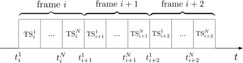
Figure 1: Considered slotted time frame structure.

II-A Data Generation Models

For the considered grant-free transmission scenario, each user tries to deliver one update to the base station in each time frame. When the users’ updates are generated depends on which of the following two data generation models is used [21].

II-A1 Generate-at-request (GAR)

For GAR, the base station requests all users to simultaneously generate their updates at the beginning of each time frame. GAR is applicable to many important IoT applications, such as structural health monitoring and autonomous driving.

II-A2 Generate-at-will (GAW)

For GAW, a user’s update is generated right before its transmit time slot. GAW has been commonly used in the AoI literature, since it ensures that the delivered updates are freshly generated.

In this paper, GAR will be focused on due to the following two reasons. First, the AoI expression for grant-free transmission for GAW can be straightforwardly obtained from that for GAR, as shown in the next section. Second, if there are retransmissions within one time frame, GAW requires a user to repeatedly generate updates, and hence, causes a higher energy consumption than GAR. For grant-based transmission, this increase in energy consumption is not severe since the number of retransmissions in one frame is small [21]. However, in the grant-free case, a user might have to carry out a large number of retransmissions due to potential collisions, which means that GAW can cause a significantly higher energy consumption than GAR.

II-B Channel Access Modes

II-B1 Orthogonal Multiple Access (OMA)

Based on OMA, a user’s transmission can be successful only if it solely occupies the bandwidth resource block, i.e., a time slot. A simple example of OMA based grant-free transmission is slotted ALOHA, as described in the following.

Prior to ${\rm TS}_{i}^{n}$, assume that $j$ users have successfully delivered their updates to the base station. For grant-free transmission, each of the remaining $M-j$ users will independently make a transmission attempt with the same transmit power, denoted by $P$, and the same transmission probability, denoted by $\mathbb{P}_{\rm TX}$. $\mathbb{P}_{\rm TX}$ can be based on a fixed choice, or be state-dependent, i.e., $\mathbb{P}_{j}=\frac{1}{M-j}$ [35]. It is assumed that the base station can inform the users about the outcome of their updates via a dedicated control channel.

There are three possible events which cause an update failure for a user: i) the user does not make a transmission attempt; ii) a collision occurs, i.e., there are more than one concurrent transmissions; iii) an outage occurs due to the user’s weak channel condition, i.e., $\log(1+P|h_{m}^{i,n}|^{2})\leq R$, where $R$ denotes the user’s target data rate, and $h_{m}^{i,n}$ denotes ${\rm U}_{m}$’s channel gain in ${\rm TS}_{i}^{n}$. In this paper, all users are assumed to have the identical target data rates, and their channel gains are assumed to be independent and identically complex Gaussian distributed with zero mean and unit variance.

II-B2 Non-orthogonal Multiple Access (NOMA)

With NOMA, a user can still succeed in its updating, even if multiple users choose the same time slot. Recall that the principle of NOMA can be implemented in different forms. For the purpose of illustration, a particular form of NOMA, termed NOMA-assisted random access, is adopted to reduce the AoI of grant-free transmission [29]. In particular, prior to transmission, the base station configures $K$ receive SNR levels, denoted by $P_{1}\geq\cdots\geq P_{K}$. If ${\rm U}_{m}$ chooses $P_{k}$ during ${\rm TS}_{i}^{n}$, it will scale its transmitted signal by $\sqrt{\frac{P_{k}}{|h_{m}^{i,n}|^{2}}}$. The base station carries out SIC by decoding the signal delivered at SNR level, $P_{k}$, before decoding the one at $P_{k+1}$, $1\leq k\leq K-1$. The SNR levels are preconfigured to guarantee the success of SIC, i.e., the following conditions need to be satisfied:

$$\log\left(1+\frac{P_{k}}{1+(M-1)P_{k+1}}\right)=R,\quad 1\leq k\leq K-1,$$ (1)

and $\log\left(1+P_{K}\right)=R$, which means $P_{K}=2^{R}-1$ and $P_{k}=\left(2^{R}-1\right)\left(1+(M-1)P_{k+1}\right)$, where the noise power is assumed to be normalized to one. We note that the condition in (1) is stricter than the condition $\log\left(1+\frac{P_{k}}{1+\sum_{i=k+1}^{K}P_{i}}\right)=R$, and ensures the success of SIC, even if one user chooses $P_{k}$ and the remaining users choose the SNR level which contributes the most interference, i.e., $P_{k+1}$. We further note that the case in which all $M-1$ remaining users choose $P_{k+1}$ is the worst case, since some users may choose SNR levels other than $P_{k+1}$ or even decide not to transmit at all.

Again assume that there are $j$ users which have successfully sent their updates to the base station prior to ${\rm TS}_{i}^{n}$. Each of the remaining $M-j$ users will first randomly choose an SNR level with equal probability, denoted by $\mathbb{P}_{k}=\frac{1}{K}$, and independently make a transmission attempt with probability $\mathbb{P}_{\rm TX}$. For illustrative purposes, assume that ${\rm U}_{m}$ is among the $M-j$ remaining users, and chooses $P_{k}$. The possible events which cause ${\rm U}_{m}$’s update to fail are listed as follows:

• The user does not make an attempt for transmission;

• The receive SNR level chosen by the user is not feasible due to the user’s transmit power budget, i.e., $P_{k}$ is not feasible for ${\rm U}_{m}$ in ${\rm TS}_{i}^{n}$ if $\frac{P_{k}}{|h_{m}^{i,n}|^{2}}>P$;

• Another user also chooses $P_{k}$, which leads to a collision at $P_{k}$ and hence a failure at the $k$-th stage of SIC;

• Prior to the $k$-th stage of SIC, SIC has already been terminated due to one or more failures in the previous SIC stages.

We note that for both the OMA and NOMA cases, a user keeps re-sending its update to the base station until either the user succeeds or the time frame is finished.

II-C AoI Model

AoI is an important performance metric for quantifying the freshness of the updates delivered to the base station. We note that for the considered grant-free scenario, all the users experience the same AoI. Therefore, without loss of generality, ${\rm U}_{1}$’s instantaneous AoI at time $t$ is focused on and defined as follows [18]:

$$\Delta(t)=t-T(t),$$ (2)

where $T(t)$ denotes the generation time of ${\rm U}_{1}$’s freshest update successfully delivered to the base station. ${\rm U}_{1}$’s average AoI of the considered network is given by

$$\bar{\Delta}=\underset{T_{\Delta}\rightarrow\infty}{\lim}\frac{1}{T_{\Delta}}\int^{T_{\Delta}}_{0}\Delta(t)dt.$$ (3)

The AoI achieved by OMA and NOMA assisted grant-free transmission will be analyzed in the following section.

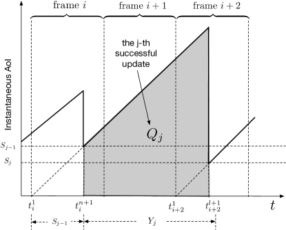
Figure 2: Illustration of AoI evolution with grant-free transmission for GAR.

III AoI of Grant-Free Transmission

As discussed in the previous section, ${\rm U}_{1}$ is treated as the tagged user and its AoI will be focused on in this section, without loss of generality. For the example shown in Fig. 2, ${\rm U}_{1}$ successfully sends its updates to the base station in ${\rm TS}_{n}^{i}$ of frame $i$ and ${\rm TS}_{l}^{i+2}$ of frame $i+2$, but fails in frame $i+1$. For the AoI analysis, the following metrics are required:

• $S_{j}$: The time duration between the generation time and the receive time of the $j$-th successful update. For the example shown in Fig. 2, $S_{j-1}=nT$ and $S_{j}=lT$.

• $Y_{j}$: The time duration between the $(j-1)$-th and the $j$-th successful updates. For the example shown in Fig. 2, $Y_{j}=(N-n)T+NT+lT$.

• $X_{j}$: The number of frames between the $(j-1)$-th and the $j$-th successful updates. An example of $X_{j}=2$ is shown in Fig. 2.

We note that in the literature of random access, $S_{j}$ is termed the service delay and $Y_{j}$ is termed the inter-departure time [35].

By using the aforementioned metrics, for GAR, ${\rm U}_{1}$’s averaged AoI is given by

$$\bar{\Delta}= \underset{J\rightarrow\infty}{\lim}\frac{\sum^{J}_{j=1}Q_{j}}{\sum^{J}_{j=1}Y_{j}}=\underset{J\rightarrow\infty}{\lim}\frac{\sum^{J}_{j=1}\left(S_{j-1}Y_{j}+\frac{1}{2}Y_{j}^{2}\right)}{\sum^{J}_{j=1}Y_{j}}=\frac{\mathcal{E}\{S_{j-1}Y_{j}\}}{\mathcal{E}\{Y_{j}\}}+\frac{\mathcal{E}\{Y_{j}^{2}\}}{2\mathcal{E}\{Y_{j}\}},$$ (4)

where $J$ denotes the total number of successful updates, $Q_{j}$ denotes the area of the shaded region shown in Fig. 2, $\mathcal{E}\{Y_{j}^{2}\}=\underset{J\rightarrow\infty}{\lim}\frac{\sum^{J}_{j=1}Y_{j}^{2}}{J}$, $\mathcal{E}\{Y_{j}\}=\underset{J\rightarrow\infty}{\lim}\frac{\sum^{J}_{j=1}Y_{j}}{J}$, and $\mathcal{E}\{\cdot\}$ denotes the expectation.

Remark 1: We note that the AoI expressions in (4) of this paper and [35, Eq. (3)] are consistent. The reason why there is an extra factor of $\frac{1}{2}$ in [35, Eq. (3)] is that the users’ instantaneous AoI was assumed to be discrete-valued in [35], instead of continuous-valued as in this paper.

Remark 2: For GAW, the user’s averaged AoI is given by

$$\bar{\Delta}^{\rm GAW}= \underset{J\rightarrow\infty}{\lim}\frac{\sum^{J}_{j=1}\left(TY_{j}+\frac{1}{2}Y_{j}^{2}\right)}{\sum^{J}_{j=1}Y_{j}}=T+\frac{\mathcal{E}\{Y_{j}^{2}\}}{2\mathcal{E}\{Y_{j}\}},$$ (5)

which is simpler than the AoI expression in (4). Therefore, the analytical results developed for GAR are straightforwardly applicable to the case for GAW.

III-A Generic Expressions for $\mathcal{E}\{S_{j-1}Y_{j}\}$, $\mathcal{E}\{Y_{j}\}$, and $\mathcal{E}\{Y_{j}^{2}\}$

As shown in (4), the AoI is a function of $\mathcal{E}\{S_{j-1}Y_{j}\}$, $\mathcal{E}\{Y_{j}\}$, and $\mathcal{E}\{Y_{j}^{2}\}$, and generic expressions for these metrics have been derived in [35], and will be briefly introduced in this subsection. In particular, the considered grant-free transmission can be modelled by a Markov chain with $M+1$ states, denoted by $s_{k}$, $0\leq k\leq M$. In particular, $s_{k}$, $0\leq k\leq M-1$, denotes the transient state, where $k$ users, other than ${\rm U}_{1}$, have successfully delivered their updates to the base station. $s_{M}$ means that ${\rm U}_{1}$ has successfully delivered its update to the base station. Define the state transition probability from $s_{j}$ to $s_{i}$ by $P_{j,i}$, $0\leq i,j\leq M$. Build an $M\times M$ matrix, denoted by $\mathbf{P}$, whose element in the $(i+1)$-th column and the $(j+1)$-th row is $P_{j,i}$, $0\leq i,j\leq M-1$. Furthermore, build an $M\times 1$ vector, denoted by $\mathbf{p}$, whose $(j+1)$-th element is $P_{j,M}$. Once $\mathbf{P}$ and $\mathbf{p}$ are available, $\mathcal{E}\{S_{j-1}Y_{j}\}$, $\mathcal{E}\{Y_{j}\}$, and $\mathcal{E}\{Y_{j}^{2}\}$ can be obtained as follows.

Denote by $Z$ the number of time slots required by ${\rm U}_{1}$ to successfully deliver its update to its base station. Then, the probability mass function (pmf) of $Z$ is given by

$$\mathbb{P}\left(Z=n\right)=\mathbf{s}_{0}^{T}\mathbf{P}_{M}^{n-1}\mathbf{p},\quad n=1,2,\cdots,$$ (6)

where $\mathbf{s}_{0}=\begin{bmatrix}1&\mathbf{0}_{1\times(M-1)}\end{bmatrix}^{T}$ denotes the initial probability vector and $\mathbf{0}_{m\times n}$ denotes an all-zero $m\times n$ matrix. Therefore, the probability that ${\rm U}_{1}$ cannot complete an update within one frame is given by $P_{\rm fail}=\mathbb{P}\left(Z>N\right)=\mathbf{s}_{0}^{T}\mathbf{P}_{M}^{N}\mathbf{1}$, where $\mathbf{1}$ denotes an $M\times 1$ all-one vector. Therefore, the pmf of access delay, $S_{j}$, can be written as follows:

$$\mathbb{P}(S_{j}=nT)=\frac{\mathbb{P}\left(Z=n\right)}{1-P_{\rm fail}}=\frac{\mathbf{s}_{0}^{T}\mathbf{P}_{M}^{n-1}\mathbf{p}}{1-\mathbf{s}_{0}^{T}\mathbf{P}_{M}^{N}\mathbf{1}},$$ (7)

for $1\leq n\leq N$, which means $\mathcal{E}\{S_{j}\}=T\sum^{N}_{n=1}n\frac{\mathbf{s}_{0}^{T}\mathbf{P}_{M}^{n-1}\mathbf{p}}{1-\mathbf{s}_{0}^{T}\mathbf{P}_{M}^{N}\mathbf{1}}$ and $\mathcal{E}\{S_{j}^{2}\}=T^{2}\sum^{N}_{n=1}n^{2}\frac{\mathbf{s}_{0}^{T}\mathbf{P}_{M}^{n-1}\mathbf{p}}{1-\mathbf{s}_{0}^{T}\mathbf{P}_{M}^{N}\mathbf{1}}$.

Similarly, the pmf of $X_{j}$ is given by

$$\mathbb{P}(X_{j}=n)=P_{\rm fail}^{n-1}(1-P_{\rm fail}),$$ (8)

which means that $\mathcal{E}\{X_{j}\}=\frac{1}{1-P_{\rm fail}}$ and $\mathcal{E}\{X_{j}^{2}\}=\frac{1+P_{\rm fail}}{\left(1-P_{\rm fail}\right)^{2}}$. The expressions of $\mathcal{E}\{X_{j}\}$ and $\mathcal{E}\{X_{j}^{2}\}$ can be used to evaluate $\mathcal{E}\{Y_{j}\}$ and $\mathcal{E}\{Y_{j}^{2}\}$, since $\mathcal{E}\{Y_{j}\}=TN\mathcal{E}\{X_{j}\}$ and $\mathcal{E}\{Y_{j}^{2}\}=N^{2}T^{2}\mathcal{E}\left\{X_{j}^{2}\right\}+2\mathcal{E}\left\{S_{j}^{2}\right\}-2\mathcal{E}\left\{S_{j}\right\}^{2}$. Furthermore, $\mathcal{E}\{S_{j}\}$, $\mathcal{E}\{S_{j}^{2}\}$, and $\mathcal{E}\{Y_{j}\}$ can be used to evaluate $\mathcal{E}\{S_{j-1}Y_{j}\}$ which can be expressed as follows:

$$\mathcal{E}\{S_{j-1}Y_{j}\}= \mathcal{E}\{S_{j}\}\mathcal{E}\{Y_{j}\}-\mathcal{E}\{S_{j}^{2}\}+\mathcal{E}\{S_{j}\}^{2},$$

where the last step follows by the fact that $S_{j-1}$ and $Y_{j}-(NT-S_{j-1})$ are independent.

As discussed above, the crucial step to evaluate the AoI is to find $\mathbf{P}$ and $\mathbf{p}$, which depends on the used multiple access schemes.

III-B OMA-Based Grant-Free Transmission

The state transition probabilities for the OMA case can be straightforwardly obtained, as shown in the following. With OMA, a single user can be served in each time slot, which means that the number of successful users after one time slot can be increased by one at most. Therefore, most of the state transition probabilities in matrix $\mathbf{P}$ are zero, except for $P_{j,j}$, $P_{j,j+1}$, and $P_{j,M}$, $0\leq j\leq M-1$. In particular, $P_{j,j}$ denotes the probability of the event that no user succeeds, and is given by [35]

$$P_{j,j}=1-(M-j)\mathbb{P}_{\rm TX}e^{-\frac{\epsilon}{P}}\left(1-\mathbb{P}_{\rm TX}\right)^{M-j-1},$$ (9)

where $\epsilon=2^{R}-1$. $P_{j,j+1}$ denotes the probability of the event that a single user, but not ${\rm U}_{1}$, succeeds and is given by

$$P_{j,j+1}=(M-j-1)\mathbb{P}_{\rm TX}e^{-\frac{\epsilon}{P}}\left(1-\mathbb{P}_{\rm TX}\right)^{M-j-1}.$$ (10)

Furthermore, the $j$-th element of $\mathbf{p}$, denoted by $P_{j,M}$, is given by

$$P_{j,M}=\mathbb{P}_{\rm TX}e^{-\frac{\epsilon}{P}}\left(1-\mathbb{P}_{\rm TX}\right)^{M-j-1}.$$ (11)

III-C NOMA-Based Grant-Free Transmission

The benefit of using NOMA is that more users can be admitted simultaneously than for OMA. In particular, with NOMA, the number of successful users after one time slot can be increased by $K$ at most, whereas the number of successful users was no more than $1$ for OMA. This means that the non-zero state transition probabilities in matrix $\mathbf{P}$ include $P_{j,j}$, $P_{j,j+i}$, and $P_{j,M}$, $0\leq j\leq M-1$, $1\leq i\leq K$ and $j+i\leq M-1$.

The analysis of the state transition probabilities for the NOMA case is more challenging than that for the OMA case, mainly due to the application of SIC. For example, a collision at SNR level $P_{k}$ can prevent all those users, which choose SNR level $P_{i}$, $i>k$, from being successful. The following lemma provides a high-SNR approximation for the state transition probabilities.

$\mathbf{Lemma}$ 1.

At high SNR, the state transition probability, $P_{j,j}$, $0\leq j\leq M-1$, can be approximated as follows:

$$P_{j,j}\approx 1-\sum^{M-j}_{m=1}{M-j\choose m}\mathbb{P}_{\rm TX}^{m}(1-\mathbb{P}_{\rm TX})^{M-j-m}$$ (12)

$$\times\sum_{k=1}^{K}m\mathbb{P}_{K}\left(1-k\mathbb{P}_{K}\right)^{m-1},$$

the state transition probability, $P_{j,j+1}$, $0\leq j\leq M-2$, can be approximated as follows:

$$P_{j,j+1}\approx (M-j)\mathbb{P}_{\rm TX}(1-\mathbb{P}_{\rm TX})^{M-j-1}\frac{M-j-1}{M-j}K\mathbb{P}_{K}$$

$$+\sum^{M-j}_{m=2}{M-j\choose m}\mathbb{P}_{\rm TX}^{m}(1-\mathbb{P}_{\rm TX})^{M-j-m}\sum^{K-1}_{k=1}\frac{M-j-1}{M-j}m\mathbb{P}_{K}$$ (13)

$$\left[(1-k\mathbb{P}_{K})^{m-1}-\sum^{K}_{\kappa=k+1}(m-1)\mathbb{P}_{K}(1-\kappa\mathbb{P}_{K})^{m-2}\right],$$

and the state transition probability, $P_{j,j+i}$, $0\leq j\leq M-3$ and $2\leq i\leq\min\{M-1-j,K\}$, can be approximated as follows:

$$P_{j,j+i} \approx{M-j\choose i}\mathbb{P}_{\rm TX}^{i}(1-\mathbb{P}_{\rm TX})^{M-j-i}\sum^{K-i+1}_{k_{1}=1}\sum^{K}_{k_{2}=k_{1}+i-1}\frac{M-j-i}{M-j}\mathbb{P}_{K}^{i}{k_{2}-k_{1}-1\choose i-2}\prod^{i}_{p=1}p$$

$$+\sum^{M-j}_{m=i+1}{M-j\choose m}\mathbb{P}_{\rm TX}^{m}(1-\mathbb{P}_{\rm TX})^{M-j-m}$$

$$\times\sum^{K-i}_{k_{1}=1}\sum^{K-1}_{k_{2}=k_{1}+i-1}\frac{M-j-i}{M-j}\mathbb{P}_{K}^{i}{k_{2}-k_{1}-1\choose i-2}\prod^{i-1}_{p=0}(m-p)$$

$$\times\left[(1-k_{2}\mathbb{P}_{K})^{m-i}-\sum^{K}_{\kappa=k_{2}+1}(m-i)\mathbb{P}_{K}(1-\kappa\mathbb{P}_{K})^{m-i-1}\right].$$ (14)

Proof.

See Appendix A. ∎

Once the transition probability matrix $\mathbf{P}$ is obtained, the elements of $\mathbf{p}$ can be obtained straightforwardly by applying $\mathbf{P}\mathbf{1}+\mathbf{p}=\mathbf{1}$, where recall that $\mathbf{1}$ denotes an $M\times 1$ all-one vector.

The closed-form analytical expressions shown in Lemma 1 allow the evaluation of the impact of NOMA on the AoI without carrying out intensive Monte Carlo simulations. However, the expressions of the state transition probabilities shown in Lemma 1 are quite involved, which makes it difficult to obtain insights about the performance difference between OMA and NOMA. For this reason, the special case of $K=2$ and $N=1$ is focused on in the remainder of this section. $K=2$ means that there are two SNR levels, i.e., the base station needs to carry out two-stage SIC only, which is an important case in practice due to its low system complexity. $N=1$ implies that there is one time slot in each frame, i.e., in each time slot, all users have updates to deliver and hence always participate in contention.

For this case, the following lemma provides the optimal choice for the transmission probability $\mathbb{P}_{\rm TX}$.

$\mathbf{Lemma}$ 2.

For the special case of $K=2$ and $N=1$, the optimal choice for the transmission probability $\mathbb{P}_{\rm TX}$ is given by

$$\mathbb{P}_{\rm TX}^{*}=\frac{\eta}{M},$$ (15)

for $M\rightarrow\infty$ and $P\rightarrow\infty$, where $\eta$ is the root of the following equation: $\left(1-\frac{\eta}{2}\right)e^{-\frac{\eta}{2}}+\left(1-\frac{\eta^{2}}{2}\right)e^{-\eta}=0$.

Proof.

See Appendix B. ∎

Remark 3: Note that $\left(1-\frac{\eta}{2}\right)e^{-\frac{\eta}{2}}+\left(1-\frac{\eta^{2}}{2}\right)e^{-\eta}=0$ is not related to $M$, which means that $\eta$ is not a function of $M$. By applying off-shelf root solvers, the exact value of $\eta$ can be straightforwardly obtained as follows: $\eta\approx 1.6646$.

By using Lemma 2, the AoI performance difference between NOMA and OMA is analyzed in the following proposition.

Proposition 1.

For the special case of $K=2$ and $N=1$, for $M\rightarrow\infty$ and $P\rightarrow\infty$, the ratio between the AoI achieved by NOMA and OMA is given by

$$\frac{\bar{\Delta}^{N}}{\bar{\Delta}^{O}}\approx\frac{2e^{\eta-1}}{\eta\left(e^{\frac{\eta}{2}}+1+\frac{\eta}{2}\right)},$$ (16)

where $\bar{\Delta}^{N}$ and $\bar{\Delta}^{O}$ denote the AoI achieved by NOMA and OMA, respectively.

Proof.

See Appendix C. ∎

Remark 4: Recall that $\eta\approx 1.6646$, which means that the ratio in Proposition 1 is $\frac{\bar{\Delta}^{N}}{\bar{\Delta}^{O}}\approx 0.5653$, i.e., the use of NOMA can almost halve the AoI achieved by OMA. We note that this significant performance gain is achieved by using NOMA with two SNR levels only, i.e., the simplest form of NOMA. By implementing NOMA with more than two SNR levels, the performance gain of NOMA over OMA can be further increased, as shown in the next section.

Remark 5: As shown in the proof for Proposition 1, the optimal choice of $\mathbb{P}_{\rm TX}$ for OMA is $\frac{1}{M}$. This is expected as explained in the following. With $M$ users competing for access in a single channel, the use of a transmission probability of $\frac{1}{M}$ is reasonable. By using the same rationale, one might expect that $\frac{2}{M}$ should be optimal for the NOMA transmission probability with two SNR levels. However, Lemma 2 shows that the optimal value of $\mathbb{P}_{\rm TX}$ is $\frac{1.6646}{M}$, which is a more conservative choice for transmission than $\frac{2}{M}$. The reason for this are potential SIC errors. In particular, although there are two channels (or two SNR levels, $P_{1}$ and $P_{2}$), a collision at $P_{1}$ causes SIC to immediately terminate, which means that $P_{2}$ can no longer be used to serve any users, i.e., the number of the effective channels is less than $2$.

Remark 6: Motivated by the results shown in Lemma 2 and Proposition 1, for the general case of $K>2$, a simple choice of $\mathbb{P}_{\rm TX}=\min\left\{1,\frac{K}{M}\right\}$ can be used for NOMA. In fact, the simulation results presented in the next section show that this choice is sufficient to realize a significant performance gain of NOMA over OMA. We note that this choice of $\mathbb{P}_{\rm TX}$ depends on $M$ only, unlike the the state-dependent choice of $\mathbb{P}_{\rm TX}$ used for OMA, which is $\mathbb{P}_{\rm TX}=\frac{1}{M-j}$ [35]. Therefore, an important direction for future research is to find a more sophisticated state-dependent choice of $\mathbb{P}_{\rm TX}$ for NOMA-assisted grant-free transmission.

Remark 7: Proposition 1 implies that the application of NOMA is particularly beneficial for grant-free transmission, compared to its application to grant-based transmission. Recall that in grant-based networks, one important benefit of using NOMA for AoI reduction is that a user can be scheduled to transmit earlier than with OMA [21]. However, for a user which has already been scheduled to transmit early in OMA, the impact of NOMA on the user’ AoI can be insignificant, particularly at high SNR. Unlike grant-based networks, Proposition 1 shows that in grant-free networks, the use of NOMA can reduce the AoI of OMA by more than $40\%$, and this significant performance gain applies for all users in the network.

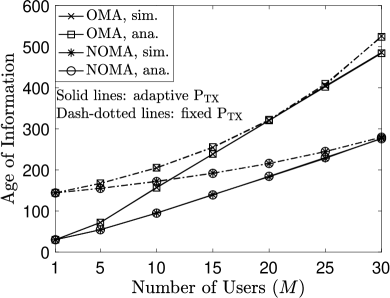
(a) With Two SNR Levels ($K=2$)

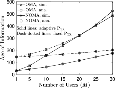
(b) With Four SNR Levels ($K=4$)

Figure 3: Impact of the number of users on the average AoI achieved with OMA and NOMA assisted grant-free transmission for GAR. $T=6$, $P=20$ dB, $R=0.5$ BPCU, and $N=8$. For the fixed choice of $\mathbb{P}_{\rm TX}$, $\mathbb{P}_{\rm TX}=0.05$, and for the adaptive choice of $\mathbb{P}_{\rm TX}$, $\mathbb{P}_{\rm TX}=\min\left\{1,\frac{K}{M}\right\}$ for NOMA, and $\mathbb{P}_{\rm TX}=\frac{1}{M-j}$ for OMA, i.e., a state-dependent choice is used for OMA as discussed in Section II-B.

IV Simulation Results

In this section, simulation results are presented to demonstrate the AoI achieved by the considered grant-free transmission schemes and to also verify the developed analytical results.

In Fig. 3, the impact of the number of users on the average AoI achieved by the considered grant-free transmission schemes is investigated. As can be seen from the figure, the AoI achieved with NOMA is significantly lower than that of OMA. In addition, Fig. 3 demonstrates that the performance gain of NOMA over OMA increases as the number of users, $M$, grows. This observation can be explained by using Proposition 1 which states that, for $K=2$, $N=1$, $M\rightarrow\infty$ and $P\rightarrow\infty$, $\bar{\Delta}^{N}\approx 0.5653\bar{\Delta}^{O}$, or equivalently $\bar{\Delta}^{N}-\bar{\Delta}^{O}\approx 0.4347\bar{\Delta}^{O}$. Because increasing $M$ increases $\bar{\Delta}^{O}$, the performance gain of NOMA over OMA also increases as the number of users grows. Therefore, the use of NOMA is particularly important for grant-free transmission with a massive number of users, an important use case for 6G. Between the two choices of $\mathbb{P}_{\rm TX}$, the adaptive choice yields a better AoI than the fixed choice. For the two subfigures in Fig. 3, different numbers of SNR levels, $K$, are used. By comparing the two subfigures, one can observe that the AoI achieved by the NOMA scheme can be reduced by increasing the number of SNR levels. This is because the use of more SNR levels makes user collisions less likely to happen. Fig. 3 also demonstrates the accuracy of the AoI expressions developed in Lemma 1.

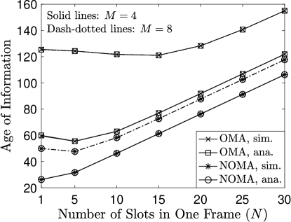
Figure 4: Impact of the number of time slots in each frame on the average AoI achieved by the OMA and NOMA assisted grant-free transmission schemes for GAR. $K=4$, $T=6$, $P=20$ dB, $R=0.5$ BPCU, $M=8$, and the adaptive choices for $\mathbb{P}_{\rm TX}$ are used.

In Fig. 4, the impact of the number of time slots in each frame, $N$, on the average AoI achieved by the two considered grant-free transmission schemes is studied. As can be seen from the figure, the use of NOMA can always realize lower AoI than OMA, regardless of the choices of $N$. An interesting observation from Fig. 4 is that a small increase of $N$, e.g., from $1$ to $5$, can reduce the AoI. This is because the likelihood for users to deliver their updates to the base station is improved if there are more time slots in each frame. However, after $N\geq 10$, further adding more time slots in each frame increases the AoI, which can be explained with the following example. Assume that ${\rm U}_{1}$ can always successfully update its base station in the first time slot of each frame. For this example, ${\rm U}_{1}$’s AoI is simply the length of one time frame, and hence its AoI is increased if there are more time slots in one frame.

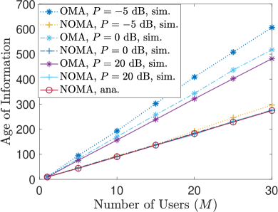
(a) $R=0.1$ BPCU

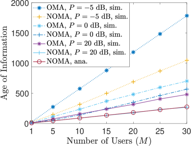
(b) $R=0.5$ BPCU

Figure 5: AoI performance achieved by the two grant-free transmission schemes for the special case with $K=2$ and $N=1$, where $T=6$, and the optimal choices of $\mathbb{P}_{\rm TX}$ are used.

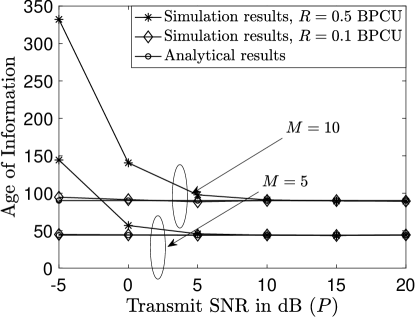
Figure 6: Illustration of the accuracy of the developed high-SNR analytical results. $K=2$, $N=1$, $T=6$, and the optimal choices of $\mathbb{P}_{\rm TX}$ are used.

As discussed in the previous section, the special case with $K=2$ and $N=1$ is important in practice, and hence the AoI realized by the OMA and NOMA assisted grant-free transmission schemes is investigated in Fig. 5. In particular, the figure shows that the performance gain of NOMA over OMA is particularly large at low SNR. This is a valuable property in practice since most AoI sensitive applications, such as IoT and sensor networks, are energy constrained and operate in the low SNR regime. Fig. 5(a) also demonstrates that for the case with small $R$, even if the SNR is low, i.e., $-5$ and $0$ dB, the difference between the analytical and simulation results is negligible. This property of the developed analytical results is particularly important, given the fact that, for many important applications of grant-free transmission, such as IoT and uMTC, the users’ target data rates are indeed small. The aforementioned conclusions are also confirmed by Fig. 6, where the AoI is shown as a function of the transmit SNR. In particular, the developed analytical results provide accurate estimates in the medium-to-high SNR regions regardless of the choices of $R$.

In Fig. 7, the AoI of grant-free transmission is shown as a function of the transmission probability, $\mathbb{P}_{\rm TX}$, and the figure demonstrates that the choices of $\mathbb{P}_{\rm TX}$ are crucial to the AoI performance of grant-free transmission. Furthermore, Fig. 7 shows that NOMA assisted grant-free transmission always yields a smaller AoI than the OMA case, if the same values for the transmission probability are used for both of the schemes. As shown in Lemma 2 and the proof for Proposition 1, $\mathbb{P}_{\rm TX}=\frac{1}{M}$ is optimal for OMA, and $\mathbb{P}_{\rm TX}=\frac{\eta}{M}$ is optimal for NOMA in the case with $K=2$ and $N=1$. Fig. 7 verifies the optimality of these choices of $\mathbb{P}_{\rm TX}$, since the minimal AoIs achieved by the fixed choices of $\mathbb{P}_{\rm TX}$ match perfectly with the AoIs realized by the optimal choices of $\mathbb{P}_{\rm TX}$.

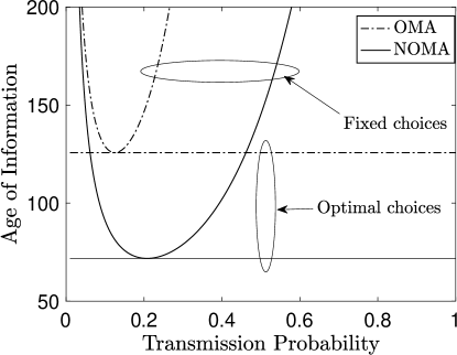
Figure 7: Illustration of the impact of $\mathbb{P}_{\rm TX}$ on the AoI achieved by the considered grant-free schemes for GAR. $T=6$, $P=20$ dB, $R=0.5$ BPCU, $K=2$, $N=1$, and $M=8$.

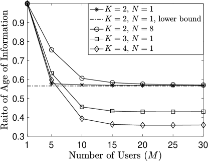
Figure 8: Impact of the number of users on the ratio between the AoI achieved with the NOMA and OMA, i.e., $\frac{\bar{\Delta}^{N}}{\bar{\Delta}^{O}}$, for GAR. $T=6$, $P=20$ dB, $R=0.5$ BPCU, and the optimal choices of $\mathbb{P}_{\rm TX}$ are used.

In Fig. 8, the performance of the considered OMA and NOMA grant-free schemes are compared by using the following AoI ratio, $\frac{\bar{\Delta}^{N}}{\bar{\Delta}^{O}}$. For the special case of $N=1$ and $K=2$, Proposition 1 predicts that this ratio is $0.5653$ for large $M$, which is confirmed by Fig. 8. If $K$ is fixed, i.e., $K=2$, an increase of $N$ does not change the ratio significantly, particularly in the case of large $M$. By introducing more SNR levels, i.e., increasing $K$, the AoI ratio can be further reduced, which means that the performance gain of NOMA over OMA can be increased by introducing more SNR levels. This is expected since increasing $K$ reduces the likelihood of user collisions and ensures that users can update the base station earlier.

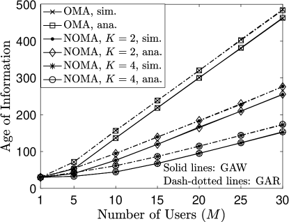
Figure 9: AoI achieved by the considered grant-free transmission schemes for different data generation models. $N=8$, $T=6$, $R=0.5$ BPCU, and the adaptive choices of $\mathbb{P}_{\rm TX}$ are used.

For all the previous simulation results, GAR has been considered, which means that a user’s update is generated at the beginning of a time frame, instead of at the beginning of a time slot as for GAW. In Fig. 9, the AoI achieved by the considered grant-free transmission schemes for the two different data generation models is illustrated. As can be seen from the figure, for both GAR and GAW, NOMA assisted grant-free transmission always outperforms the OMA based scheme. In addition, the figure shows that the AoI realized by the considered schemes for GAW is smaller than that for GAR, because, for GAW, each update is generated right before its delivery time, i.e., there is no service delay $S_{j}$. We also note that the difference between the AoI for GAW and GAR is not significant, but the use of GAW can cause a higher energy consumption than GAR, since GAW requires a user to re-generate an update for each retransmission.

V Conclusions

In this paper, the impact of NOMA on the AoI of grant-free transmission has been investigated by applying a particular form of NOMA, namely NOMA-assisted random access. By modelling grant-free transmission as a Markov chain and accounting for SIC, closed-form analytical expressions for the AoI achieved by NOMA assisted grant-free transmission have been obtained, and asymptotic studies have been carried out to demonstrate that the use of the simplest form of NOMA is already sufficient to reduce the AoI of OMA by more than $40\%$. In addition, the developed analytical results have also been shown useful for optimizing the users’ transmission probabilities, $\mathbb{P}_{\rm TX}$, which is crucial for performance maximization of grant-free transmission.

In this paper, concise and insightful analytical results have been developed for the special case of $N=1$. An important direction for future research is the development of similar insightful results for the general case of $N\geq 1$. We also note that the use of NOMA may reduce a user’s energy consumption by avoiding the possible large number of retransmissions needed for OMA; however, a user that chooses a high receive SNR level, e.g., $P_{1}$, may consume more energy than in OMA. Therefore, another important direction for future research is to study how to realize a balanced tradeoff between energy efficiency and AoI reduction.

VI Acknowledgements

The authors thank Dr. Jinho Choi for his kind suggestions about the implementation of NOMA assisted random access.

Appendix A Proof for Lemma 1

The proof is divided into three parts to evaluate $P_{j,j}$, $P_{j,j+1}$, and $P_{j,j+i}$, $i\geq 2$, respectively. Throughout the proof, the high SNR assumption is made, which ensures that all the SNR levels, $P_{k}$, $1\leq k\leq K$, are feasible for each user, i.e., transmission failures are due to user collisions only. The users’ channel gains in different time slots are assumed to be independent and identically complex Gaussian distributed with zero mean and unit variance.

A-A Evaluating $P_{j,j}$

To find the expression for $P_{j,j}$, assume that $j$ users have successfully delivered their updates to the base station. Therefore, each of the remaining $M-j$ users independently makes an attempt to transmit with the probability, $\mathbb{P}_{\rm TX}$, at a randomly chosen SNR level. $P_{j,j}$ is the probability of the event that none of the $M-j$ users succeeds.

Define $E_{P_{k}|j}$ as the event that given $M-j$ remaining users, a user successfully updates the base station by using the $k$-th SNR level, $P_{k}$, and no user succeeds at $P_{i}$, $i<k$. The reason to include the constraint that no user succeeds at $P_{i}$, $i<k$, in the definition of $E_{P_{k}|j}$ is to ensure that $E_{P_{k}|j}$ and $E_{P_{p}|j}$, $k<p$, are uncorrelated. For example, the event that ${\rm U}_{i}$ succeeds by using $P_{2}$ and ${\rm U}_{j}$ succeeds by using $P_{3}$ belongs to $E_{P_{2}|j}$ only, and is not included in $E_{P_{3}|j}$ .

Therefore, the probability $P_{j,j}$ can be expressed as follows:

$$P_{j,j}= 1-\mathbb{P}\left(E_{P_{1}|j}\cup\cdots\cup E_{P_{K}|j}\right)$$ (17)

$$= 1-\sum^{K}_{k=1}\mathbb{P}\left(E_{P_{k}|j}\right).$$

Further define $E_{m|j}$ as the event that among the $M-j$ remaining users, there are $m$ active users which make the transmission attempts, and define $E_{P_{k}|m}$ as the event that among the $m$ active users, a single user successfully updates the base station by using the $k$-th SNR level, $P_{k}$, and no user chooses $P_{i}$, $i<k$, which means

$$P_{j,j}= 1-\sum^{K}_{k=1}\sum^{M-j}_{m=1}{M-j\choose m}\mathbb{P}\left(E_{m|j}\right)\mathbb{P}\left(E_{P_{k}|m}\right).$$ (18)

By using the transmission attempt probability of $\mathbb{P}_{\rm TX}$, the probability, $E_{m|j}$, can be obtained as follows:

$$\mathbb{P}(E_{m|j})=\mathbb{P}_{\rm TX}^{m}(1-\mathbb{P}_{\rm TX})^{M-j-m}.$$ (19)

Without loss of generality, assume that ${\rm U}_{i}$ is one of the $m$ active users which make transmission attempts. The probability for the event that ${\rm U}_{i}$ chooses $P_{k}$, and no user chooses $P_{i}$, $i<k$, is given by

$$\mathbb{P}_{K}\left(1-k\mathbb{P}_{K}\right)^{m-1},$$ (20)

where $(1-k\mathbb{P}_{K})$ is the probability of the event that a user which is not ${\rm U}_{i}$ cannot choose $P_{p}$, $1\leq p\leq k$. Therefore, $\mathbb{P}\left(E_{P_{k}|j,m}\right)$ can be approximated as follows:

$$\mathbb{P}\left(E_{P_{k}|m}\right)\approx m\mathbb{P}_{K}\left(1-k\mathbb{P}_{K}\right)^{m-1},$$ (21)

since each of the $m$ active users can be the successful user with the equal probability, where the high SNR assumption is used, i.e., all SNR levels are feasible to each user and only the errors caused by user collisions are considered. By combining (18), (19), and (21), $P_{j,j}$ can be expressed as follows:

$$P_{j,j}\approx 1-\sum^{M-j}_{m=1}{M-j\choose m}\mathbb{P}_{\rm TX}^{m}(1-\mathbb{P}_{\rm TX})^{M-j-m}$$ (22)

$$\times\sum_{k=1}^{K}m\mathbb{P}_{K}\left(1-k\mathbb{P}_{K}\right)^{m-1}.$$

A-B Evaluating $P_{j,j+1}$

Recall that $P_{j,j+1}$ is also conditioned on the assumption that $j$ users have successfully updated the base station, and $P_{j,j+1}$ is the probability of the event that there is a single successful update from a user which cannot be ${\rm U}_{1}$.

Define $E^{1}_{P_{k}|j}$ as the event that given $M-j$ remaining users, a single user, other than ${\rm U}_{1}$, successfully updates the base station by using the $k$-th SNR level. At high SNR, the following two conclusions can be made regarding $E^{1}_{P_{k}|j}$. On the one hand, due to the feature of SIC, $E^{1}_{P_{k}|j}$ implies that no user chooses $P_{i}$, $i<k$, which can be shown by contradiction. Assume that ${\rm U}_{p}$ chooses $P_{i}$. If ${\rm U}_{p}$ is the only user choosing $P_{i}$, ${\rm U}_{p}$ becomes an additional successful user, which contradicts the assumption that there is a single successful user. If multiple users choose $P_{i}$, a collision occurs and SIC needs to be terminated at $P_{i}$, which contradicts the assumption that a successful update happens at $P_{k}$. On the other hand, $E^{1}_{P_{k}|j}$ does not exclude the event that an SNR level, $P_{i}$, $i>k$, is chosen by a user; however, $E^{1}_{P_{k}|j}$ does imply that if $P_{i}$, $i>k$, is chosen, a collision must happen at this SNR level, otherwise there will be an additional successful user. We also note that $E^{1}_{P_{k}|j}$ is different from $E_{P_{k}|j}$ for the following two reasons. First, $E_{P_{k}|j}$ does not exclude the event that the successful user is ${\rm U}_{1}$. Second, for $E_{P_{k}|j}$, it is still possible for a user to succeed at SNR levels, $P_{i}$, $i>k$.

By using $E^{1}_{P_{k}|j}$, the probability $P_{j,j+1}$ can be expressed as follows:

$$P_{j,j+1}= \mathbb{P}(E^{1}_{L_{1}|j}\cup\cdots\cup E^{1}_{L_{K}|j})=\sum^{K}_{k=1}\mathbb{P}(E^{1}_{L_{k}|j}),$$ (23)

where the last step follows by the fact that the $E^{1}_{P_{k}|j}$, $1\leq k\leq K$, are uncorrelated.

Similar to $E_{P_{k}|m}$, define $E^{1}_{P_{k}|m}$ as the event that among the $m$ active users, a single user, other than ${\rm U}_{1}$, successfully updates the base station by using the $k$-th SNR level. By using $E_{m|j}$ and $E^{1}_{P_{k}|m}$, $P_{j,j+1}$ can be expressed as follows:

$$P_{j,j+1}= \sum^{K}_{k=1}\sum^{M-j}_{m=1}{M-j\choose m}\mathbb{P}\left(E_{m|j}\right)\mathbb{P}\left(E_{P^{1}_{k}|m}\right).$$ (24)

The analysis of $\mathbb{P}\left(E_{P^{1}_{k}|m}\right)$ is challenging. First, we assume that $m\geq 2$, i.e., there are more than one active users. For illustrative purposes, assume that ${\rm U}_{2}$ is an active user. Denote by $E^{+}_{2k}$ the event that ${\rm U}_{2}$ succeeds by using $P_{k}$, and $\mathbb{P}\left(E^{+}_{2k}\right)$ is given by

$$\mathbb{P}\left(E^{+}_{2k}\right)\approx\mathbb{P}_{K}(1-k\mathbb{P}_{K})^{m-1},$$ (25)

where the high SNR approximation is used, and the reason to have $(1-k\mathbb{P}_{K})^{m-1}$ is that the $k$ highest SNR levels are no longer available to the other $m-1$ active users. Because $m\geq 2$, $k\leq K-1$, i.e., ${\rm U}_{2}$ cannot succeed by using $P_{K}$, which can be explained by using a simple example with ${\rm U}_{2}$ and ${\rm{U}_{3}}$ being the active users ($m=2$). As discussed previously, if ${\rm U}_{2}$ chooses $P_{K}$, ${\rm{U}_{3}}$ has to choose $P_{p}$, $p>K$, which is not possible.

Furthermore, denote by $E^{-}_{2k}$ the event that ${\rm U}_{2}$ succeeds by using $P_{k}$, and there is at least one additional user which succeeds by using $P_{i}$, $i\geq k+1$. $\mathbb{P}\left(E^{-}_{2k}\right)$ is given by

$$\mathbb{P}\left(E^{-}_{2k}\right)\approx\mathbb{P}_{K}\sum^{K}_{\kappa=k+1}(m-1)\mathbb{P}_{K}(1-\kappa\mathbb{P}_{K})^{m-2},$$ (26)

which is obtained in a similar manner as $\mathbb{P}\left(E_{P_{k}|m}\right)$ in (21).

By using $E^{+}_{2k}$ and $E^{-}_{2k}$, the probability for the event that among the $m$ active users, only ${\rm U}_{2}$ succeeds by using $P_{k}$, denoted by $E_{2k}$, is given by

$$\mathbb{P}\left(E_{2k}\right)= \mathbb{P}\left(E^{+}_{2k}\right)-\mathbb{P}\left(E^{-}_{2k}\right)\approx\mathbb{P}_{K}\left[(1-k\mathbb{P}_{K})^{m-1}-\sum^{K}_{\kappa=k+1}(m-1)\mathbb{P}_{K}(1-\kappa\mathbb{P}_{K})^{m-2}\right].$$ (27)

Intuitively, $\mathbb{P}\left(E_{P^{1}_{k}|m}\right)$ should be simply $\mathbb{P}\left(E_{P^{1}_{k}|m}\right)=(m-1)\mathbb{P}\left(E_{2k}\right)$, i.e., including $(m-1)$ cases corresponding to ${\rm U}_{i}$, $2\leq i\leq m$. If ${\rm U}_{1}$ is one of the active users, indeed, $\mathbb{P}\left(E_{P^{1}_{k}|m}\right)=(m-1)\mathbb{P}\left(E_{2k}\right)$. However, if ${\rm U}_{1}$ is not an active user, $\mathbb{P}\left(E_{P^{1}_{k}|m}\right)=m\mathbb{P}\left(E_{2k}\right)$. Therefore, by taking into account the fact that ${\rm U}_{1}$ might not be an active user, $\mathbb{P}\left(E_{P^{1}_{k}|m}\right)$ can be expressed as follows:

$$\mathbb{P}\left(E_{P^{1}_{k}|m}\right)\approx \left[\frac{m}{M-j}(m-1)+\frac{M-j-m}{M-j}(m)\right]\mathbb{P}\left(E_{2k}\right)$$ (28)

$$= \frac{M-j-1}{M-j}m\mathbb{P}_{K}\left[(1-k\mathbb{P}_{K})^{m-1}-\sum^{K}_{\kappa=k+1}(m-1)\mathbb{P}_{K}(1-\kappa\mathbb{P}_{K})^{m-2}\right],$$

for the case $m\geq 2$.

For the case $m=1$, i.e., there is a single active user, $\mathbb{P}\left(E_{P^{1}_{k}|m}\right)$ is simply zero if this user is ${\rm U}_{1}$. Otherwise, $\mathbb{P}\left(E_{P^{1}_{k}|m}\right)=\mathbb{P}_{K}$, i.e., $P_{k}$ is selected by the active user. Therefore, for $m=1$, $\mathbb{P}\left(E_{P^{1}_{k}|m}\right)$ is given by

$$\mathbb{P}\left(E_{P^{1}_{k}|m}\right)\approx\frac{M-j-1}{M-j}\mathbb{P}_{K}.$$ (29)

By combining (24), (28) and (29), the probability, $P_{j,j+1}$, can be obtained as shown in the lemma.

A-C Evaluating $P_{j,j+i}$, $i\geq 2$

We note that for $P_{j,j+1}$, there is a single successful update, and $P_{j,j+1}$ has been analyzed by first specifying which SNR level, i.e., $P_{k}$, is used for this successful update. The same method could be applied to analyze $P_{j,j+i}$, $i\geq 2$; however, the resulting expression can be extremely complicated if the number of the used SNR levels is large.

Instead, the feature of SIC can be used to simplify the analysis of $P_{j,j+i}$. Consider the following example with $i=3$ and $K=8$. Assume that the following three SNR levels, $P_{2}$, $P_{4}$, and $P_{5}$, are used by the successful users. The key observation for simplifying the performance analysis is that those SNR levels prior to $P_{2}$ and between the chosen ones are not selected by any users, e.g., no user chooses $P_{1}$ and $P_{3}$. This observation can be explained by taking $P_{3}$ as an example. If this SNR level has been selected, a collision must happen at this level, otherwise there should be an additional successful user. However, if a collision does happen at $P_{3}$, SIC needs to be terminated in the third SIC stage, and hence no successful update can happen at $P_{4}$, which contradicts to the assumption that $P_{4}$ is used by a successful user. As a result, no one chooses $P_{3}$.

By using this observation, we note that only two SNR levels are significant to the analysis of $P_{j,j+i}$, namely the highest and the lowest SNR levels, which are denoted by $P_{k_{1}}$ and $P_{k_{2}}$, respectively. For the aforementioned example, $P_{k_{1}}=P_{2}$ and $P_{k_{2}}=P_{5}$. Define $E^{i}_{P_{k}|j}$ as the event that given $M-j$ remaining users, $i$ users which are not ${\rm U}_{1}$ successfully update the base station, where $P_{k_{1}}$ and $P_{k_{2}}$ are the highest and lowest used SNR levels. By using $E^{i}_{P_{k}|j}$, the probability $P_{j,j+i}$ can be expressed as follows:

$$P_{j,j+i}= \sum^{K-i+1}_{k_{1}=1}\sum^{K}_{k_{2}=k_{1}+i-1}\mathbb{P}(E^{i}_{L_{k}|j})=\sum^{K-i+1}_{k_{1}=1}\sum^{K}_{k_{2}=k_{1}+i-1}\sum^{M}_{m=1}{M-j\choose m}\mathbb{P}\left(E_{m|j}\right)\mathbb{P}\left(E_{P^{i}_{k}|m}\right),$$ (30)

where $E_{P^{i}_{k}|m}$ is defined similar to $E^{i}_{P_{k}|j}$ with the assumption that there are $m$ active users.

In order to find $\mathbb{P}\left(E_{P^{i}_{k}|m}\right)$, again, we first focus on the case $m\geq i+1$, i.e., there are more than $i$ active user. Define $E_{ik}$ as the probability for the particular event that among the $m$ active users, ${\rm U}_{2}$ succeeds by using $P_{k_{1}}$, ${\rm U}_{j}$ succeeds by using $P_{k_{1}+j-2}$, $3\leq j\leq i$, and ${\rm U}_{i+1}$ succeeds by using $P_{k_{2}}$. Similar to $\mathbb{P}\left(E_{2k}\right)$, $\mathbb{P}\left(E_{ik}\right)$ can be approximated at high SNR as follows:

$$\mathbb{P}\left(E_{ik}\right)\approx\mathbb{P}_{K}^{i}\left[(1-k_{2}\mathbb{P}_{K})^{m-i}-\sum^{K}_{\kappa=k_{2}+1}(m-i)\mathbb{P}_{K}(1-\kappa\mathbb{P}_{K})^{m-i-1}\right],$$ (31)

where the term, $(1-k_{2}\mathbb{P}_{K})^{m-i}$, is due to the fact that the remaining $m-i$ active users can choose $P_{i}$, $i>k_{2}$, only, and the second term in the bracket is obtained similar to $\mathbb{P}\left(E_{P_{k}|m}\right)$ in (21).

Following steps similar to those to obtain $\mathbb{P}\left(E_{P^{1}_{k}|m}\right)$ in (28), $\mathbb{P}\left(E_{P^{i}_{k}|m}\right)$ can be obtained from $\mathbb{P}\left(E_{ik}\right)$ as follows:

$$\mathbb{P}\left(E_{P^{i}_{k}|m}\right)\approx \mathbb{P}\left(E_{ik}\right){k_{2}-k_{1}-1\choose i-2}\underset{\text{repetitions if the tagged user is one of the $m$ active users }}{\underbrace{\left[\frac{m}{M-j}(m-1)(m-2)\cdots(m-i)+\right.}}$$ (32)

$$\underset{\text{repetitions if the tagged user is not one of the $m$ active users}}{\underbrace{\left.\frac{M-j-m}{M-j}m(m-1)\cdots(m-i+1)\right]}}$$

$$= \mathbb{P}\left(E_{ik}\right){k_{2}-k_{1}-1\choose i-2}\frac{M-j-i}{M-j}m\cdots(m-i+1),$$

for the case $m\geq i+1$, where ${k_{2}-k_{1}-1\choose i-2}$ is the number of the possible choices for the $(i-2)$ SNR levels which are between $P_{k_{1}}$ and $P_{k_{2}}$.

The special case $m=i$ means that there are $m$ active users and each of the active users is a successful user. Therefore, the probability in (31), $\mathbb{P}\left(E_{ik}\right)$, is simply $\mathbb{P}_{K}^{i}$, and hence for the case $m=i$, $\mathbb{P}\left(E_{P^{i}_{k}|m}\right)$ can be expressed as follows:

$$\mathbb{P}\left(E_{P^{i}_{k}|m}\right)\approx\mathbb{P}_{K}^{i}{k_{2}-k_{1}-1\choose i-2}\frac{M-j-i}{M-j}i\cdots 1.$$ (33)

By combining (32) and (33), the expression of $P_{j,j+i}$ can be obtained as shown in the lemma. Therefore, the proof for the lemma is complete.

Appendix B Proof for Lemma 2

The proof comprises first simplifying the state transition probabilities, then developing an asymptotic expression of the AoI, and finally finding the optimal choice of $\mathbb{P}_{\rm TX}$.

B-A Simplifying the State Transition Probabilities

For the case of $N=1$ and $K=2$, only the following transition probabilities, $P_{0,0}$, $P_{0,1}$, $P_{0,2}$, need to be focused on.

In particular, the expression of $P_{0,0}$ can be simplified as follows:

$$P_{0,0}\approx 1-\sum^{M}_{m=1}{M\choose m}\mathbb{P}_{\rm TX}^{m}(1-\mathbb{P}_{\rm TX})^{M-m}\sum_{k=1}^{K}m\mathbb{P}_{K}\left(1-k\mathbb{P}_{K}\right)^{m-1}$$

$$\overset{(1)}{=} 1-\sum^{M}_{m=1}{M\choose m}\mathbb{P}_{\rm TX}^{m}(1-\mathbb{P}_{\rm TX})^{M-m}m\mathbb{P}_{K}\left(1-\mathbb{P}_{K}\right)^{m-1}-M\mathbb{P}_{\rm TX}(1-\mathbb{P}_{\rm TX})^{M-1}\mathbb{P}_{K}$$

$$\overset{(b)}{=} 1-\sum^{M}_{m=1}{M\choose m}\mathbb{P}_{\rm TX}^{m}(1-\mathbb{P}_{\rm TX})^{M-m}m\mathbb{P}_{K}^{m}-M\mathbb{P}_{\rm TX}(1-\mathbb{P}_{\rm TX})^{M-1}\mathbb{P}_{K},$$

where step $(a)$ follows by the fact that $(1-K\mathbb{P}_{K})^{m-1}\neq 0$ only if $m=1$, and step $(b)$ follows by $\mathbb{P}_{K}=1-\mathbb{P}_{K}$ for $K=2$. By using the properties of the binomial coefficients, $P_{0,0}$ can be simplified as follows:

$$P_{0,0}\approx 1-M\mathbb{P}_{K}\mathbb{P}_{\rm TX}\sum^{M-1}_{i=0}{M-1\choose i}(\mathbb{P}_{K}\mathbb{P}_{\rm TX})^{i}(1-\mathbb{P}_{\rm TX})^{M-1-i}-M\mathbb{P}_{\rm TX}(1-\mathbb{P}_{\rm TX})^{M-1}\mathbb{P}_{K}$$ (34)

$$= 1-M\mathbb{P}_{K}\mathbb{P}_{\rm TX}(\mathbb{P}_{K}\mathbb{P}_{\rm TX}+1-\mathbb{P}_{\rm TX})^{M-1}-M\mathbb{P}_{\rm TX}(1-\mathbb{P}_{\rm TX})^{M-1}\mathbb{P}_{K}.$$

Similarly, for the case of $K=2$, $P_{0,1}$ can be first written as follows:

$$P_{0,1}\approx M\mathbb{P}_{\rm TX}(1-\mathbb{P}_{\rm TX})^{M-1}\frac{M-1}{M}K\mathbb{P}_{K}+\sum^{M}_{m=2}{M\choose m}\mathbb{P}_{\rm TX}^{m}(1-\mathbb{P}_{\rm TX})^{M-m}\sum^{K-1}_{k=1}\frac{M-1}{M}m\mathbb{P}_{K}$$

$$\left[(1-k\mathbb{P}_{K})^{m-1}-\sum^{K}_{\kappa=k+1}(m-1)\mathbb{P}_{K}(1-\kappa\mathbb{P}_{K})^{m-2}\right].$$ (35)

Define $\tau(m)=\sum^{K-1}_{k=1}\frac{M-1}{M}m\mathbb{P}_{K}[(1-k\mathbb{P}_{K})^{m-1}-\sum^{K}_{\kappa=k+1}(m-1)\mathbb{P}_{K}(1-\kappa\mathbb{P}_{K})^{m-2}]$. Note that in the expression of $\tau(m)$, $k\geq 1$, and hence $\kappa\geq 2$. For the case of $K=2$, $1-2\mathbb{P}_{K}=0$. By using this observation, $\tau(m)$ can be simplified as follows:

$$\tau(m)=\frac{m(M-1)}{M}\mathbb{P}_{K}(1-\mathbb{P}_{K})^{m-1},$$ (36)

for $m>2$, and

$$\tau(2)=\left(\frac{m}{M}(m-1)+\frac{M-m}{M}m\right)\mathbb{P}_{K}\left[(1-\mathbb{P}_{K})-\mathbb{P}_{K}\right]=0.$$ (37)

By using the simplified expression of $\tau(m)$, $P_{0,1}$ can be simplified as follows:

$$P_{0,1}\approx M\mathbb{P}_{\rm TX}(1-\mathbb{P}_{\rm TX})^{M-1}\frac{M-1}{M}K\mathbb{P}_{K}$$ (38)

$$+\sum^{M}_{m=3}{M\choose m}\mathbb{P}_{\rm TX}^{m}(1-\mathbb{P}_{\rm TX})^{M-m}\frac{m(M-1)}{M}\mathbb{P}_{K}(1-\mathbb{P}_{K})^{m-1}$$

$$= (M-1)\mathbb{P}_{\rm TX}(1-\mathbb{P}_{\rm TX})^{M-1}+(M-1)\sum^{M}_{m=3}{M-1\choose m-1}\mathbb{P}_{\rm TX}^{m}(1-\mathbb{P}_{\rm TX})^{M-m}\mathbb{P}_{K}^{m},$$

where the last step follows by the fact that $1-\mathbb{P}_{K}=\mathbb{P}_{K}$.

Finally, $P_{0,2}$ can rewritten as follows:

$$P_{0,2}\approx{M\choose 2}\mathbb{P}_{\rm TX}^{i}(1-\mathbb{P}_{\rm TX})^{M-2}\sum^{K-1}_{k_{1}=1}\sum^{K}_{k_{2}=k_{1}+1}\frac{M-i}{M}\mathbb{P}_{K}^{2}{k_{2}-k_{1}-1\choose 0}\prod^{1}_{p=0}(2-p)$$ (39)

$$+\sum^{M}_{m=3}{M\choose m}\mathbb{P}_{\rm TX}^{m}(1-\mathbb{P}_{\rm TX})^{M-m}\sum^{K-2}_{k_{1}=1}\sum^{K-1}_{k_{2}=k_{1}+1}\frac{M-i}{M}\mathbb{P}_{K}^{2}{k_{2}-k_{1}-1\choose 0}\prod^{1}_{p=0}(m-p)$$

$$\times\left[(1-k_{2}\mathbb{P}_{K})^{m-2}-\sum^{K}_{\kappa=k_{2}+1}(m-2)\mathbb{P}_{K}(1-\kappa\mathbb{P}_{K})^{m-3}\right]$$

$$\overset{(a)}{=}{M\choose 2}\mathbb{P}_{\rm TX}^{2}(1-\mathbb{P}_{\rm TX})^{M-2}2\frac{M-2}{M}\mathbb{P}_{K}^{2}=\frac{(M-1)!}{(M-3)!}\mathbb{P}_{\rm TX}^{2}(1-\mathbb{P}_{\rm TX})^{M-2}\mathbb{P}_{K}^{2},$$

where step $(a)$ follows by employing the properties of the binomial coefficients.

B-B Asymptotic Studies of AoI

By using the above transition probabilities, the probability for the event that ${\rm U}_{1}$ cannot complete an update within one frame, $P_{\rm fail}$, can be simplified as follows:

$$P_{\rm fail}\approx \mathbb{P}\left(Z>N\right)=\mathbf{s}_{0}^{T}\mathbf{P}_{M}^{N}\mathbf{1}=\sum^{2}_{j=0}P_{0,j}$$ (40)

$$= 1-M(x+1-\mathbb{P}_{\rm TX})^{M-1}x-M(1-\mathbb{P}_{\rm TX})^{M-1}x+2(M-1)(1-\mathbb{P}_{\rm TX})^{M-1}x$$

$$+\underset{\tau_{0}}{\underbrace{(M-1)\sum^{M}_{i=2}{M-1\choose i}(1-\mathbb{P}_{\rm TX})^{M-i-1}x^{i+1}}}+\frac{(M-1)!}{(M-3)!}(1-\mathbb{P}_{\rm TX})^{M-2}x^{2},$$

where $x=\mathbb{P}_{\rm TX}\mathbb{P}_{K}$. By using the properties of binomial coefficients, $\tau_{0}$ can be rewritten as follows:

$$\tau_{0}= x(M-1)\sum^{M}_{i=2}{M-1\choose i}(1-\mathbb{P}_{\rm TX})^{M-i-1}x^{i}$$ (41)

$$= (1-\mathbb{P}_{\rm TX}+x)^{M-1}(M-1)x-(1-\mathbb{P}_{\rm TX})^{M-1}(M-1)x$$

$$-(M-1)(1-\mathbb{P}_{\rm TX})^{M-2}(M-1)x^{2}.$$

By using the simplified expression of $\tau_{0}$, $P_{\rm fail}$ can be rewritten as follows:

$$P_{\rm fail}\approx 1-M(x+1-\mathbb{P}_{\rm TX})^{M-1}x-M(1-\mathbb{P}_{\rm TX})^{M-1}x+2(M-1)(1-\mathbb{P}_{\rm TX})^{M-1}x$$

$$+(1-\mathbb{P}_{\rm TX}+x)^{M-1}(M-1)x-(1-\mathbb{P}_{\rm TX})^{M-1}(M-1)x$$

$$-(M-1)(1-\mathbb{P}_{\rm TX})^{M-2}(M-1)x^{2}+(M-1)(M-2)(1-\mathbb{P}_{\rm TX})^{M-2}x^{2}$$

$$= 1-(\mathbb{P}_{\rm TX}\mathbb{P}_{K}+1-\mathbb{P}_{\rm TX})^{M-1}\mathbb{P}_{\rm TX}\mathbb{P}_{K}-(1-\mathbb{P}_{\rm TX}+(M-1)\mathbb{P}_{\rm TX}\mathbb{P}_{K})(1-\mathbb{P}_{\rm TX})^{M-2}\mathbb{P}_{\rm TX}\mathbb{P}_{K}.$$

The simplified expression of $P_{\rm fail}$ can be used to facilitate the asymptotic studies of the AoI. For the case of $N=1$, the pmf of the access delay can be obtained from $P_{\rm fail}$ as follows:

$$\mathbb{P}(S_{j}=T)=\frac{\mathbf{s}_{0}^{T}\mathbf{P}_{M}^{0}\mathbf{p}}{1-\mathbf{s}_{0}^{T}\mathbf{P}_{M}\mathbf{1}}=\frac{p_{0,M}}{p_{0,M}}=1,$$ (42)

where $p_{0,M}$ is the first element of $\mathbf{p}$. As a result, $\mathcal{E}\{S_{j}\}$ and $\mathcal{E}\{S_{j}^{2}\}$ can be obtained as follows:

$$\mathcal{E}\{S_{j}\}=T\sum^{1}_{n=1}n\frac{\mathbf{s}_{0}^{T}\mathbf{P}_{M}^{n-1}\mathbf{p}}{1-\mathbf{s}_{0}^{T}\mathbf{P}_{M}^{N}\mathbf{1}}=T,$$ (43)

and

$$\mathcal{E}\{S_{j}^{2}\}=T^{2}\sum^{1}_{n=1}n^{2}\frac{\mathbf{s}_{0}^{T}\mathbf{P}_{M}^{n-1}\mathbf{p}}{1-\mathbf{s}_{0}^{T}\mathbf{P}_{M}^{N}\mathbf{1}}=T^{2},$$ (44)

which are expected since $S_{j}$ becomes a deterministic parameter for this special case.

Furthermore, recall that the inter-departure time $Y_{j}$ can be rewritten as follows:

$$Y_{j}=\left(NT-S_{j-1}\right)+(X_{j}-1)NT+S_{j}.$$ (45)

Therefore, for the case of $N=1$, the expectation of $Y_{j}$ can be simplified as follows:

$$\mathcal{E}\{Y_{j}\}= \mathcal{E}\{\left(NT-S_{j-1}\right)+(X_{j}-1)NT+S_{j}\}$$ (46)

$$= TN\mathcal{E}\{X_{j}\}=TN\frac{1}{1-P_{\rm fail}},$$

which is obtained by using the fact that $X_{j}$ follows the geometric distribution. Similarly, the expectation of $Y_{j}^{2}$ can be simplified as follows:

$$\mathcal{E}\{Y_{j}^{2}\}= N^{2}T^{2}\mathcal{E}\left\{X_{j}^{2}\right\}+2\mathcal{E}\left\{S_{j}^{2}\right\}-2\mathcal{E}\left\{S_{j}\right\}^{2}=N^{2}T^{2}\frac{1+P_{\rm fail}}{\left(1-P_{\rm fail}\right)^{2}}+2T^{2}-2T^{2}.$$ (47)

Finally, for the case of $N=1$, the averaged AoI can be expressed as follows:

$$\bar{\Delta}^{N}= \frac{\mathcal{E}\{S_{j}\}\mathcal{E}\{Y_{j}\}-\mathcal{E}\{S_{j}^{2}\}+\mathcal{E}\{S_{j}\}^{2}}{\mathcal{E}\{Y_{j}\}}+\frac{\mathcal{E}\{Y_{j}^{2}\}}{2\mathcal{E}\{Y_{j}\}}=\frac{T\mathcal{E}\{Y_{j}\}-T^{2}+T^{2}}{\mathcal{E}\{Y_{j}\}}+\frac{\mathcal{E}\{Y_{j}^{2}\}}{2\mathcal{E}\{Y_{j}\}}$$ (48)

$$= T+\frac{N^{2}T^{2}\frac{1+P_{\rm fail}}{\left(1-P_{\rm fail}\right)^{2}}}{2TN\frac{1}{1-P_{\rm fail}}}\approx T+\frac{NT(2-f(\mathbb{P}_{\rm TX}))}{2f(\mathbb{P}_{\rm TX})},$$

where $f(\mathbb{P}_{\rm TX})=(\mathbb{P}_{\rm TX}\mathbb{P}_{K}+1-\mathbb{P}_{\rm TX})^{M-1}\mathbb{P}_{\rm TX}\mathbb{P}_{K}+(1-\mathbb{P}_{\rm TX}+(M-1)\mathbb{P}_{\rm TX}\mathbb{P}_{K})(1-\mathbb{P}_{\rm TX})^{M-2}\mathbb{P}_{\rm TX}\mathbb{P}_{K}$.

B-C Finding the Optimal Choice of $\mathbb{P}_{\rm TX}$

The considered AoI minimization problem can be expressed as follows: $\underset{0\leq\mathbb{P}_{\rm TX}\leq 1}{\min}\bar{\Delta}^{N}$. It is challenging to show whether $\bar{\Delta}^{N}$ is a convex function of $\mathbb{P}_{\rm TX}$, given the complex expression of $\bar{\Delta}^{N}$. However, it can be shown that $\bar{\Delta}^{N}$ first decreases and then increases as $\mathbb{P}_{\rm TX}$ grows, as shown in the following.

The first order derivative of $\bar{\Delta}^{N}$ with respect to $\mathbb{P}_{\rm TX}$ is given by

$$\left(\bar{\Delta}^{N}\right)^{\prime}\approx \frac{NT}{2}\left(\frac{-f^{\prime}(\mathbb{P}_{\rm TX})}{f(\mathbb{P}_{\rm TX})}-\frac{2f^{\prime}(\mathbb{P}_{\rm TX})^{\prime}-f(\mathbb{P}_{\rm TX})f^{\prime}(\mathbb{P}_{\rm TX})}{f^{2}(\mathbb{P}_{\rm TX})}\right)=-\frac{NT}{2}\frac{2f^{\prime}(\mathbb{P}_{\rm TX})}{f^{2}(\mathbb{P}_{\rm TX})},$$

which shows that the monotonicity of $\bar{\Delta}^{N}$ is decided by the sign of $f^{\prime}(\mathbb{P}_{\rm TX})$ only. In the following, we will first show that $f^{\prime}(\mathbb{P}_{\rm TX})=0$ has a single root for $0\leq\mathbb{P}_{\rm TX}\leq 1$.

With some straightforward algebraic manipulations, $f^{\prime}(\mathbb{P}_{\rm TX})$ can be expressed as follows:

$$f^{\prime}(\mathbb{P}_{\rm TX})= \left[1-M\frac{\mathbb{P}_{\rm TX}}{2}\right]\left(1-\frac{\mathbb{P}_{\rm TX}}{2}\right)^{M-2}+\left[1-2\mathbb{P}_{\rm TX}-M(M-3)\frac{\mathbb{P}_{\rm TX}^{2}}{2}\right]\left(1-\mathbb{P}_{\rm TX}\right)^{M-3}.$$ (49)

Because $0\leq\mathbb{P}_{\rm TX}\leq 1$, both $\left(1-\frac{\mathbb{P}_{\rm TX}}{2}\right)$ and $\left(1-\mathbb{P}_{\rm TX}\right)$ are positive.

On the one hand, if $\mathbb{P}_{\rm TX}\geq\frac{2}{M}$, $1-M\frac{\mathbb{P}_{\rm TX}}{2}\leq 0$, otherwise $1-M\frac{\mathbb{P}_{\rm TX}}{2}\geq 0$. On the other hand, there are two roots for $1-2\mathbb{P}_{\rm TX}-M(M-3)\frac{\mathbb{P}_{\rm TX}^{2}}{2}=0$, namely $\frac{\sqrt{4+2M(M-1)}-4}{M(M-3)}$ and $\frac{-\sqrt{4+2M(M-1)}-4}{M(M-3)}$. When $M\rightarrow\infty$, the two roots can be approximated as follows:

$$\frac{\pm\sqrt{4+2M(M-1)}-4}{M(M-3)} \approx\pm\frac{\sqrt{2}}{M}.$$ (50)

Therefore, $1-2\mathbb{P}_{\rm TX}-M(M-3)\frac{\mathbb{P}_{\rm TX}^{2}}{2}\leq 0$ if $\mathbb{P}_{\rm TX}\geq\frac{\sqrt{2}}{M}$, otherwise $1-2\mathbb{P}_{\rm TX}-M(M-3)\frac{\mathbb{P}_{\rm TX}^{2}}{2}>0$. Denote the root(s) of $f^{\prime}(\mathbb{P}_{\rm TX})=0$ by $\mathbb{P}_{\rm TX}^{*}$, which is bounded as follows:

$$\frac{\sqrt{2}}{M}\leq\mathbb{P}_{\rm TX}^{*}\leq\frac{2}{M}.$$ (51)

A key observation from (51) is that the upper and lower bounds on $\mathbb{P}_{\rm TX}^{*}$ are of the same order of $\frac{1}{M}$. Therefore, $\mathbb{P}_{\rm TX}^{*}$ can be expressed as $\mathbb{P}_{\rm TX}^{*}=\frac{\eta}{M}$, where $\sqrt{2}\leq\eta\leq 2$. By using this expression for $\mathbb{P}_{\rm TX}^{*}$, $f^{\prime}(\mathbb{P}^{*}_{\rm TX})=0$ can be expressed as follows:

$$0= \left(1-\frac{\eta}{2}\right)\left(1-\frac{\eta}{2M}\right)^{M-2}+\left(1-2\frac{\eta}{M}-(M-3)\frac{\eta^{2}}{2M}\right)\left(1-\frac{\eta}{M}\right)^{M-3}.$$ (52)

In order to find an explicit expression of $\mathbb{P}_{\rm TX}^{*}$, we note that $f_{x}(x)=\left(1-\frac{a}{x}\right)^{x}$ can be approximated at $x\rightarrow\infty$ as follows:

$$\ln f_{x}(x)= \underset{x\rightarrow\infty}{\lim}x\ln\left(1-\frac{a}{x}\right)=\underset{z\rightarrow 0}{\lim}\frac{\ln\left(1-az\right)}{z}=-\underset{z\rightarrow 0}{\lim}\frac{a}{1-az}=-a,$$ (53)

which implies $\left(1-\frac{a}{M}\right)^{M}=e^{-a}$ for large $M$.

Therefore, for $M\rightarrow\infty$, (52) can be approximated as follows:

$$0= \left(1-\frac{\eta}{2}\right)e^{-\frac{\eta}{2}}+\left(1-\frac{\eta^{2}}{2}\right)e^{-\eta},$$ (54)

where the value of $\eta$ can be straightforwardly obtained by applying off-the-shelf root solvers. It is important to point out that (54) has a single root, which means that $\mathbb{P}_{\rm TX}^{*}=\frac{\eta}{M}$ is the single root of $f^{\prime}(\mathbb{P}_{\rm TX})=0$. Therefore, $\mathbb{P}_{\rm TX}^{*}=\frac{\eta}{M}$ is the optimal choice of $\mathbb{P}_{\rm TX}$ to minimize $\bar{\Delta}^{N}$, and the proof is complete.

Appendix C Proof for Proposition 1

Based on Lemma 2, the optimal choice for the transmission probability is given by $\mathbb{P}_{\rm TX}^{*}=\frac{\eta}{M}$. By using this optimal choice of $\mathbb{P}_{\rm TX}$, $P_{\rm fail}$ can be expressed as follows:

$$P_{\rm fail}\approx 1-\left(1-\frac{\eta}{2M}\right)^{M-1}\frac{\eta}{2M}-\left(1-\frac{\eta}{M}+(M-1)\frac{\eta}{2M}\right)\left(1-\frac{\eta}{M}\right)^{M-2}\frac{\eta}{2M}.$$ (55)

Again applying the following limit: $\underset{M\rightarrow\infty}{\lim}\left(1-\frac{a}{M}\right)^{M}=e^{-a}$, $P_{\rm fail}$ can be approximated for large $M$ as follows:

$$P_{\rm fail}\approx 1-e^{-\frac{\eta}{2}}\frac{\eta}{2M}-\left(1-\frac{\eta}{M}+(M-1)\frac{\eta}{2M}\right)e^{-\eta}\frac{\eta}{2M}\approx 1-e^{-\frac{\eta}{2}}\frac{\eta}{2M}-\left(1+\frac{\eta}{2}\right)e^{-\eta}\frac{\eta}{2M}.$$ (56)

By using this approximation of $P_{\rm fail}$, the AoI achieved by NOMA can be approximated as follows:

$$\bar{\Delta}^{N}\approx T+\frac{NT}{2}\frac{2-e^{-\frac{\eta}{2}}\frac{\eta}{2M}-\left(1+\frac{\eta}{2}\right)e^{-\eta}\frac{\eta}{2M}}{e^{-\frac{\eta}{2}}\frac{\eta}{2M}+\left(1+\frac{\eta}{2}\right)e^{-\eta}\frac{\eta}{2M}}$$ (57)

$$\approx \eta+\frac{NT}{2}\left(\frac{2}{e^{-\frac{\eta}{2}}\frac{\eta}{2M}+\left(1+\frac{\eta}{2}\right)e^{-\eta}\frac{\eta}{2M}}-1\right)\approx NT\frac{2Me^{\eta}}{\eta\left(e^{\frac{\eta}{2}}+1+\frac{\eta}{2}\right)}.$$

In order to find an explicit expression for the AoI achieved by OMA for the case of $N=1$, the transition probabilities can be expressed as follows:

$$P_{0,0}=1-M\mathbb{P}_{\rm TX}\left(1-\mathbb{P}_{\rm TX}\right)^{M-1},$$ (58)

and

$$P_{0,1}=(M-1)\mathbb{P}_{\rm TX}\left(1-\mathbb{P}_{\rm TX}\right)^{M-1}.$$ (59)

Therefore, for OMA, the failure probability, $P_{\rm fail}$, is given by

$$P_{\rm fail}= P_{0,0}+P_{0,1}=1-\mathbb{P}_{\rm TX}\left(1-\mathbb{P}_{\rm TX}\right)^{M-1}.$$ (60)

By using the expression for $P_{\rm fail}$, the AoI achieved by OMA can be expressed as follows:

$$\bar{\Delta}^{O}= 1+\frac{NT(1+P_{\rm fail})}{2(1-P_{\rm fail})}=1+\frac{NT\left(2-\mathbb{P}_{\rm TX}\left(1-\mathbb{P}_{\rm TX}\right)^{M-1}\right)}{2\mathbb{P}_{\rm TX}\left(1-\mathbb{P}_{\rm TX}\right)^{M-1}}.$$ (61)

Define $f_{O}(\mathbb{P}_{\rm TX})=\mathbb{P}_{\rm TX}\left(1-\mathbb{P}_{\rm TX}\right)^{M-1}$. Similar to the NOMA case, it is straightforward to show that the optimal choice of $\mathbb{P}_{\rm TX}$ for OMA is the root of $f^{\prime}_{O}(\mathbb{P}_{\rm TX})=0$. Note that $f^{\prime}_{O}(\mathbb{P}_{\rm TX})$ can be expressed as follows:

$$f^{\prime}_{O}(\mathbb{P}_{\rm TX})= (1-M\mathbb{P}_{\rm TX})(1-\mathbb{P}_{\rm TX})^{M-2},$$ (62)

which is the reason why $\mathbb{P}_{\rm TX}^{*}=\frac{1}{M}$ is optimal for the OMA case. By using $\mathbb{P}_{\rm TX}^{*}=\frac{1}{M}$, $P_{\rm fail}$ can be expressed as follows: $P_{\rm fail}=1-\frac{1}{M}\left(1-\frac{1}{M}\right)^{M-1}$, and hence the AoI achieved by OMA is given by

$$\bar{\Delta}^{O}= 1+\frac{NT}{2}\frac{2-\mathbb{P}_{\rm TX}\left(1-\mathbb{P}_{\rm TX}\right)^{M-1}}{\mathbb{P}_{\rm TX}\left(1-\mathbb{P}_{\rm TX}\right)^{M-1}}=1+\frac{NT}{2}\left[\frac{2M}{\left(1-\frac{1}{M}\right)^{M-1}}-1\right].$$ (63)

For $M\rightarrow\infty$, the AoI achieved by OMA can be approximated as follows:

$$\bar{\Delta}^{O}\approx \frac{NT}{2}\frac{2M}{\left(1-\frac{1}{M}\right)^{M-1}}\approx NTMe.$$ (64)

Therefore, for $M\rightarrow\infty$, the ratio between the AoI realized by NOMA and OMA is given by

$$\frac{\bar{\Delta}^{N}}{\bar{\Delta}^{O}}\approx\frac{NT\frac{2Me^{\eta}}{\eta\left(e^{\frac{\eta}{2}}+1+\frac{\eta}{2}\right)}}{NTMe}=\frac{2e^{\eta-1}}{\eta\left(e^{\frac{\eta}{2}}+1+\frac{\eta}{2}\right)},$$ (65)

which completes the proof.

References

- [1] A. C. Cirik, N. M. Balasubramanya, L. Lampe, G. Vos, and S. Bennett, “Toward the standardization of grant-free operation and the associated NOMA strategies in 3GPP,” IEEE Commun. Standards Mag., vol. 3, no. 4, pp. 60–66, Dec. 2019.
- [2] X. You, C. Wang, J. Huang et al., “Towards 6G wireless communication networks: Vision, enabling technologies, and new paradigm shifts,” Sci. China Inf. Sci., vol. 64, no. 110301, pp. 1–74, Feb. 2021.
- [3] R. Abbas, M. Shirvanimoghaddam, Y. Li, and B. Vucetic, “Random access for M2M communications with QoS guarantees,” IEEE Trans. Commun., vol. 65, no. 7, pp. 2889–2903, Jul. 2017.
- [4] J. Choi, J. Ding, N.-P. Le, and Z. Ding, “Grant-free random access in machine-type communication: Approaches and challenges,” IEEE Wireless Commun., vol. 29, no. 1, pp. 151–158, Feb. 2022.
- [5] L. Liu and W. Yu, “Massive connectivity with massive MIMO - Part I: Device activity detection and channel estimation,” IEEE Trans. on Signal Process., vol. 66, no. 11, pp. 2933–2946, Jun. 2018.
- [6] L. Liu, E. G. Larsson, W. Yu, P. Popovski, C. Stefanovic, and E. de Carvalho, “Sparse signal processing for grant-free massive connectivity: A future paradigm for random access protocols in the internet of things,” IEEE Signal Process. Mag., vol. 35, no. 5, pp. 88–99, Sept. 2018.
- [7] K. Senel and E. G. Larsson, “Grant-free massive MTC-enabled massive MIMO: A compressive sensing approach,” IEEE Transa. Commun., vol. 66, no. 12, pp. 6164–6175, Dec. 2018.
- [8] R. Abbas, M. Shirvanimoghaddam, Y. Li, and B. Vucetic, “A novel analytical framework for massive grant-free NOMA,” IEEE Trans. Commun., vol. 67, no. 3, pp. 2436–2449, Mar. 2019.
- [9] Y. Ma, G. Ma, N. Wang, Z. Zhong, and B. Ai, “OTFS-TSMA for massive internet of things in high-speed railway,” IEEE Trans. Wireless Commun., vol. 21, no. 1, pp. 519–531, Jan. 2022.
- [10] J. Ding, D. Qu, and J. Choi, “Analysis of non-orthogonal sequences for grant-free RA with massive MIMO,” IEEE Trans. Commun., vol. 68, no. 1, pp. 150–160, Jan. 2020.
- [11] M. Elbayoumi, M. Kamel, W. Hamouda, and A. Youssef, “NOMA-assisted machine-type communications in UDN: State-of-the-art and challenges,” IEEE Commun. Surveys Tuts., vol. 22, no. 2, pp. 1276–1304, 2020.
- [12] X. Zhang, P. Fan, J. Liu, and L. Hao, “Bayesian learning-based multiuser detection for grant-free NOMA systems,” IEEE Trans. Wireless Commun., vol. 21, no. 8, pp. 6317–6328, Aug. 2022.
- [13] Z. Ding, R. Schober, P. Fan, and H. V. Poor, “Simple semi-grant-free transmission strategies assisted by non-orthogonal multiple access,” IEEE Trans. Commun., vol. 67, no. 6, pp. 4464–4478, Jun. 2019.
- [14] Q. Hu, J. Jiao, Y. Wang, S. Wu, R. Lu, and Q. Zhang, “Multi-type services coexistence in uplink NOMA for dual-layer LEO satellite constellation,” IEEE Internet of Things Journal, to appear in 2022.
- [15] K. Cao, H. Ding, B. Wang, L. Lv, J. Tian, Q. Wei, and F. Gong, “Enhancing physical layer security for IoT with non-orthogonal multiple access assisted semi-grant-free transmission,” IEEE Internet of Things Journal, to appear in 2022.
- [16] J. Chen, L. Guo, J. Jia, J. Shang, and X. Wang, “Resource allocation for irs assisted SGF NOMA transmission: A MADRL approach,” IEEE J. Sel. Areas Commun., vol. 40, no. 4, pp. 1302–1316, Apr. 2022.
- [17] Y. Liu, M. Zhao, L. Xiao, and S. Zhou, “Pilot domain NOMA for grant-free massive random access in massive MIMO marine communication system,” China Commun., vol. 17, no. 6, pp. 131–144, Jun. 2020.
- [18] Y. Sun, E. Uysal-Biyikoglu, R. D. Yates, C. E. Koksal, and N. B. Shroff, “Update or wait: How to keep your data fresh,” IEEE Trans. Inform. Theory, vol. 63, no. 11, pp. 7492–7508, Nov. 2017.
- [19] S. Kaul, R. Yates, and M. Gruteser, “Real-time status: How often should one update?” in Proc. IEEE INFOCOM, Orlando, FL, USA, May 2012.
- [20] A. A. Al-Habob, O. A. Dobre, and H. V. Poor, “Age- and correlation-aware information gathering,” IEEE Wireless Commun. Lett., vol. 11, no. 2, pp. 273–277, Feb. 2022.
- [21] Z. Ding, R. Schober, and H. V. Poor, “Age of information: Can CR-NOMA help?” IEEE Trans. Commun., Available on-line at arXiv:2209.09562, 2022.
- [22] H. Pan, J. Liang, S. C. Liew, V. C. M. Leung, and J. Li, “Timely information update with nonorthogonal multiple access,” IEEE Trans. Industrial Informatics, vol. 17, no. 6, pp. 4096–4106, Jun. 2021.
- [23] Q. Ren, T.-T. Chan, J. Liang, and H. Pan, “Age of information in SIC-based non-orthogonal multiple access,” in Proc. IEEE WCNC, Austin, TX, USA, 2022.
- [24] X. Feng, S. Fu, F. Fang, and F. R. Yu, “Optimizing age of information in RIS-assisted NOMA networks: A deep reinforcement learning approach,” IEEE Wireless Commun. Lett., to appear in 2022.
- [25] Z. Gao, A. Liu, C. Han, and X. Liang, “Non-orthogonal multiple access based average age of information minimization in LEO satellite-terrestrial integrated networks,” IEEE Trans. Green Commun. and Net., 2022.
- [26] A. Maatouk, M. Assaad, and A. Ephremides, “Minimizing the age of information: NOMA or OMA?” in Proc. IEEE INFOCOM WKSHPS), Paris, France, 2019.
- [27] J. F. Grybosi, J. L. Rebelatto, and G. L. Moritz, “Age of information of SIC-aided massive IoT networks with random access,” IEEE Internet of Things Journal, vol. 9, no. 1, pp. 662–670, Jan. 2022.
- [28] H. Zhang, Y. Kang, L. Song, Z. Han, and H. V. Poor, “Age of information minimization for grant-free non-orthogonal massive access using mean-field games,” IEEE Trans. Commun., vol. 69, no. 11, pp. 7806–7820, Nov. 2021.
- [29] J. Choi, “NOMA based random access with multichannel ALOHA,” IEEE J. Sel. Areas Commun., vol. 35, no. 12, pp. 2736–2743, Dec. 2017.
- [30] Y. Li and L. Dai, “Maximum sum rate of slotted aloha with successive interference cancellation,” IEEE Trans. Commun., vol. 66, no. 11, pp. 5385–5400, Nov. 2018.
- [31] A. K. Gupta and T. G. Venkatesh, “Design and performance evaluation of successive interference cancellation based slotted aloha MAC protocol,” Physical Commun., vol. 55, no. 12, pp. 101–109, Dec. 2022.
- [32] A. Munari, “Modern random access: An age of information perspective on irregular repetition slotted ALOHA,” IEEE Trans. Commun., vol. 69, no. 6, pp. 3572–3585, Jun. 2021.
- [33] S. Saha, V. B. Sukumaran, and C. R. Murthy, “On the minimum average age of information in IRSA for grant-free mMTC,” IEEE J. Sel. Areas Commun., vol. 39, no. 5, pp. 1441–1455, May 2021.
- [34] O. T. Yavascan and E. Uysal, “Analysis of slotted ALOHA with an age threshold,” IEEE J. Sel. Areas Commun., vol. 39, no. 5, pp. 1456–1470, May 2021.
- [35] Y. H. Bae and J. W. Baek, “Age of information and throughput in random access-based IoT systems with periodic updating,” IEEE Wireless Commun. Lett., vol. 11, no. 4, pp. 821–825, Apr. 2022.