Phase function methods for second order inhomogeneous linear ordinary differential equations

Abstract

It is well known that second order homogeneous linear ordinary differential equations with slowly varying coefficients admit slowly varying phase functions. This observation underlies the Liouville-Green method and many other techniques for the asymptotic approximation of the solutions of such equations. It is also the basis of a recently developed numerical algorithm that, in many cases of interest, runs in time independent of the magnitude of the equation’s coefficients and achieves accuracy on par with that predicted by its condition number. Here we point out that a large class of second order inhomogeneous linear ordinary differential equations can be efficiently and accurately solved by combining phase function methods for second order homogeneous linear ordinary differential equations with a variant of the adaptive Levin method for evaluating oscillatory integrals.

1 Introduction

We say that $\alpha$ is a phase function for the second order homogeneous linear ordinary differential equation

$$y^{\prime\prime}(t)+q(t)y(t)=0,\ \ \ \ \ a<t<b,$$ (1)

provided $\alpha^{\prime}$ is positive on $(a,b)$ and the functions

$$u(t)=\frac{\cos(\alpha(t))}{\sqrt{\alpha^{\prime}(t)}}\ \ \ \mbox{and}\ \ \ v(t)=\frac{\sin(\alpha(t))}{\sqrt{\alpha^{\prime}(t)}}$$ (2)

form a basis in its space of solutions. It is well known that when $q$ is a slowly varying function, (1) admits slowly varying phase functions, and that this is true even when $q$ is of large magnitude and the solutions of (1) are highly oscillatory or behave as combinations of rapidly increasing and decreasing exponential functions. This observation underlies the Liouville-Green method (see, for instance, Chapter 6 of [12] or Chapter 7 of [11]) and many other techniques for the asymptotic approximation of the solutions of such equations (for example, [14, 15, 13]).

It is also the basis of the algorithm of [2], which applies when the coefficient $q$ is positive. In this case, the solutions of (1) are oscillatory and the frequency of their oscillations grows with the magnitude of $q$. Consequently, when they are used in this regime, the running times of standard solvers for ordinary differential equations grow with the magnitude of $q$. By contrast, in many cases of interest, the numerical algorithm of [2] is able to calculate a nonoscillatory phase function for (1) with near machine precision accuracy in time independent of the magnitude of $q$. The companion paper [4] gives a bound on the complexity of the phase function produced by the algorithm of [2] under mild conditions on the coefficient $q$.

In this article, we describe a solver for second order inhomogeneous liner ordinary differential equations of the form

$$y^{\prime\prime}(t)+q(t)y(t)=f(t),\ \ \ \ \ a<t<b,$$ (3)

where $f$ is a slowly varying real-valued function and $q$ is slowly varying and positive. The algorithm of [2] is first used to construct a nonoscillatory phase function $\alpha$ such that the functions $u$ and $v$ defined via (2) form a basis in the space of the corresponding homogeneous problem (1). A particular solution of (3) is then given by the formula

$$z(t)=u(t)\int_{a}^{t}v(s)f(s)\ ds+v(t)\int_{a}^{t}u(s)f(s)\ ds,$$ (4)

and any solution of (3) is of the form

$$y(t)=c_{1}u(t)+c_{2}v(t)+z(t)$$ (5)

with $c_{1}$ and $c_{2}$ constants. We then use an adaptive Levin method, similar to that introduced in [5], to construct a sequence of auxillary functions $p_{1},\ldots,p_{m}$, defined on a partition of $[a,b]$, which allow us to efficiently evaluate the integrals appearing in (4). In many cases of interest, $\alpha$ and the sequence of functions $p_{1},\ldots,p_{m}$ can be constructed in time independent of the magnitude of $q$ and, once this has been done, constants $c_{1}$ and $c_{2}$ such that (5) satisfies essentially any reasonable boundary conditions can be readily computed.

The Levin method, which was introduced in [8], is a classical technique for evaluating integrals of the form

$$\int_{a}^{b}\exp(ig(s))f(s)\ ds$$ (6)

where $f$ is slowly varying and $g$ is real-valued and slowly varying. It was long believed that it suffers from “low-frequency breakdown,” meaning that accuracy is lost when $g^{\prime}$ is of insufficient magnitude. In [5], it is shown that, in fact, the Levin method is applicable regardless of the magnitude of $g^{\prime}$ and this observation is used to develop an adaptive integration scheme for integrals of the form (6). One of the key advantages of the resulting “adaptive Levin method” is its ability to efficiently evaluate oscillatory integrals in the presence of saddle points — that is, locations at which the first $l\geq 1$ derivatives of $g$ vanish.

Although the method of [2] can be extended to the case in which (1) has turning points (this is done in [3]), the algorithm of this paper often encounters numerical difficulties when used in this regime. They stem from the fact that one or both of the functions $u$ and $v$ must be rapidly increasing in regions in which $q$ is negative and of large magnitude, and this makes (5) a numerically unstable representation of the desired solution of (3). Of course, in many cases in which additional information about the desired solution is known a priori— for instance, if it is a linear combination of the particular solution and a solution $u$ of (1) whose magnitude does not become large — a numerically stable formula for representing the desired solution can be devised and (3) can be solved to high accuracy using a slightly modified version of the algorithm presented here.

The remainder of this paper is structured as follows. In Section 2, we discuss phase functions for second order homogeneous linear ordinary differential equations and describe the algorithm of [2] for the numerical calculation of nonoscillatory phase functions. Section 3 discusses the adaptive Levin method for the evaluation of oscillatory integrals and explains how a variant of it can be used to construct the sequence of functions $p_{1},\ldots,p_{m}$ which enable the rapid evaluation of the particular solution (4). In Section 4, we present the results of numerical experiments designed to demonstrate the properties of our approach to solving (3). We close with a few brief remarks in Section 5.

2 Phase functions for second order homogeneous linear ordinary differential equations

2.1 Kummer’s equation

It can be easily verified that if $\alpha$ is a phase function for the second order homogeneous linear ordinary differential equation (1) — so that the functions $u$ and $v$ defined in (2) form a basis in its space of solutions — then $\alpha^{\prime}$ solves

$$q(t)-(\alpha^{\prime}(t))^{2}+\frac{3}{4}\left(\frac{\alpha^{\prime\prime}(t)}{\alpha^{\prime}(t)}\right)^{2}-\frac{1}{2}\frac{\alpha^{\prime\prime\prime}(t)}{\alpha^{\prime}(t)}=0,\ \ \ \ \ a<t<b.$$ (7)

Equation (7) is often referred to as Kummer’s equation, after E. E Kummer who studied it in [7]. Kummer’s equation is strongly related to the better known Riccati equation

$$r^{\prime}(t)+(r(t))^{2}+q(t)=0,\ \ \ \ \ a<t<b,$$ (8)

satisfied by the logarithmic derivatives of the solutions of (1). In particular, if $\alpha$ is a phase function for (1), then

$$r(t)=i\alpha^{\prime}(t)-\frac{1}{2}\frac{\alpha^{\prime\prime}(t)}{\alpha^{\prime}(t)}$$ (9)

is a solution of (8).

When $q$ is positive, almost all solutions of Kummer’s equation are oscillatory. However, it was recognized long ago that there exist some solutions which can be asymptotically approximated by nonoscillatory functions, provided $q$ is slowly varying. This is the basis of many classical asymptotic techniques, including the Liouville-Green method. If $q$ is strictly positive on the interval $[a,b]$, then

$$u_{0}(t)=\frac{\cos\left(\alpha_{0}(t)\right)}{\sqrt{\alpha_{0}^{\prime}(t)}}\ \ \mbox{and}\ \ \ v_{0}(t)=\frac{\sin\left(\alpha_{0}(t)\right)}{\sqrt{\alpha_{0}^{\prime}(t)}},$$ (10)

where $\alpha_{0}$ is defined via

$$\alpha_{0}(t)=\int_{a}^{t}\sqrt{q(s)}\ ds,$$ (11)

are a pair of Liouville-Green approximates for (1). When $q$ is slowly varying, obviously so too is the function defined via (11), and this is the case regardless of the magnitude of $q$. For a careful discussion of the Liouville-Green method, including rigorous error bounds for the approximates (10), we refer the reader to Chapter 6 of [12]. A higher order asymptotic method which operates by iteratively refining the Liouville-Green phase $\alpha_{0}$ is developed in [14, 15, 13].

A theorem showing the existence of a nonoscillatory phase function for (1) in the case in which $q(t)=\lambda^{2}q_{0}(t)$ with $q_{0}$ smooth and strictly positive on $[a,b]$ appears in [4]. It applies when the function $p(x)=\widetilde{p}(t(x))$, where $p(t)$ is defined via

$$\widetilde{p}(t)=\frac{1}{q_{0}(t)}\left(\frac{5}{4}\left(\frac{q_{0}^{\prime}(t)}{q_{0}(t)}\right)^{2}-\frac{q_{0}^{\prime\prime}(t)}{q_{0}(t)}\right)=4\left(q_{0}(t)\right)^{\frac{1}{4}}\frac{d}{dt}\left(\frac{1}{\left(q_{0}(t)\right)^{\frac{1}{4}}}\right)$$ (12)

and $t(x)$ is the inverse function of

$$x(t)=\int_{a}^{t}\sqrt{q_{0}(s)}\ ds,$$ (13)

has a rapidly decaying Fourier transform. More explicitly, the theorem asserts that if the Fourier transform of $p$ satisfies a bound of the form

$$\left|\widehat{p}(\xi)\right|\leq\Gamma\exp\left(-\mu\left|\xi\right|\right),$$ (14)

then there exist functions $\nu$ and $\delta$ such that

$$\left|\nu(t)\right|\leq\frac{\Gamma}{2\mu}\left(1+\frac{4\Gamma}{\lambda}\right)\exp(-\mu\lambda),$$ (15)

$$\left|\widehat{\delta}(\xi)\right|\leq\frac{\Gamma}{\lambda^{2}}\left(1+\frac{2\Gamma}{\lambda}\right)\exp(-\mu|\xi|)$$ (16)

and

$$\alpha(t)=\lambda\sqrt{q_{0}(t)}\int_{a}^{t}\exp\left(\frac{\delta(u)}{2}\right)\ du$$ (17)

is a phase function for

$$y^{\prime\prime}(t)+\lambda^{2}\left(q_{0}(t)+\frac{\nu(t)}{4\lambda^{2}}\right)y(t)=0.$$ (18)

The definition of the function $p(x)$ is ostensibly quite complicated; however, $p(x)$ is, in fact, simply equal to twice the Schwarzian derivative of the inverse function $t(x)$ of (13). This theorem ensures that, even for relatively modest values of $\lambda$, (1) admits a phase function which is nonoscillatory for the purposes of numerical computation. Of course, when $\lambda$ is small, the frequency of oscillation of any phase function for (1) is modest.

Remark 1.

When discussing phase function for second order linear ordinary differential equations it is standard practice to restrict attention to the special form (1). This is because Kummer’s equation and the phase function $\alpha$ are invariant under the standard transformation which takes the more general ODE

$$y^{\prime\prime}(t)+p(t)y^{\prime}(t)+q(t)y(t)=0,\ \ \ \ \ a<t<b,$$ (19)

to the form (1). To see this, we suppose that $\alpha$ is a phase function for (19) so that $\alpha^{\prime}$ is positive on $(a,b)$ and

$$\sqrt{\frac{\omega(t)}{\alpha^{\prime}(t)}}\cos\left(\alpha(t)\right)\ \ \ \mbox{and}\ \ \ \sqrt{\frac{\omega(t)}{\alpha^{\prime}(t)}}\sin\left(\alpha(t)\right),$$ (20)

where

$$\omega(t)=\exp\left(-\int p(t)\ dt\right),$$ (21)

form a basis in its space of solutions. We note that by Abel’s theorem, the Wronskian of any pair of independent solutions of (19) is a constant multiple of $\omega$, and so the factors of $\sqrt{\omega(t)}$ appearing in (20) are necessary. It can be easily shown that $\alpha^{\prime}$ satisfies

$$q(t)-\frac{(p(t))^{2}}{4}-\frac{p^{\prime}(t)}{2}-(\alpha^{\prime}(t))^{2}+\frac{3}{4}\left(\frac{\alpha^{\prime\prime}(t)}{\alpha^{\prime}(t)}\right)^{2}-\frac{1}{2}\frac{\alpha^{\prime\prime\prime}(t)}{\alpha^{\prime}(t)}=0,\ \ \ \ \ a<t<b.$$ (22)

If we let

$$z(t)=\exp\left(-\frac{1}{2}\int p(t)\ dt\right)y(t),$$ (23)

where the choice of antiderivative is immaterial, then $z$ solves the second order linear ordinary differential equation

$$z^{\prime\prime}(t)+\left(q(t)-\frac{(p(t))^{2}}{4}-\frac{p^{\prime}(t)}{2}\right)z(t)=0$$ (24)

and substituting the coefficient in (24) into Kummer’s equation (7) simply yields (22).

2.2 A numerical algorithm for constructing nonoscillatory phase functions

In this subsection, we describe the numerical method of [2] for constructing a nonoscillatory phase function for equations of the form (1) in the event that the coefficient $q$ is slowly varying and positive on the interval $[a,b]$. The principal difficulty in designing such an algorithm is that while there exists a nonoscillatory solution of (7), almost all solutions of Kummer’s equation are oscillatory and some mechanism must be used to identify a nonoscillatory solution. The algorithm of [2] addresses this problem by introducing a “windowed” version of the coefficient $\widetilde{q}$ which is equal to a constant $\nu^{2}$ on the right quarter of the interval $[a,b]$ and nearly equal to the original coefficient $q$ on the left quarter of $[a,b]$. The equation

$$y^{\prime\prime}(t)+\widetilde{q}(t)y(t)=0$$ (25)

admits a nonoscillatory phase function $\widetilde{\alpha}$ which is equal to $i\nu t$ on the left quarter of $[a,b]$ and closely approximates a nonoscillatory phase function for $q$ on the right quarter of $[a,b]$. Accordingly, the algorithm solves an initial value problem for Kummer’s equation to calculate the values of a nonoscillatory phase function for (1) and its first few derivatives at the point $b$. A terminal value problem for Kummer’s equation is then solved to construct the desired phase function over the entire interval $[a,b]$.

We now give a more detailed description of the algorithm of [2]. It takes as inputs the endpoints $a$ and $b$, an external subroutine for evaluating the coefficient $q$, an integer parameter $k$ which determines the order of the piecewise Chebyshev expansions used to represent the outputs and a real-valued parameter $\epsilon$ which specifies the desired precision for the calculation. The outputs of the algorithm comprise three $k^{th}$ order piecewise Chebyshev expansions which represent the phase function $\alpha$ and its first two derivatives $\alpha^{\prime}$ and $\alpha^{\prime\prime}$. To be entirely clear, by an $k^{th}$ order piecewise Chebyshev expansions on the interval $[a,b]$, we mean a sum of the form

$$\sum_{i=1}^{m-1}\chi_{\left[x_{i-1},x_{i}\right)}(t)\sum_{j=0}^{k}c_{ij}\ T_{j}\left(\frac{2}{x_{i}-x_{i-1}}t+\frac{x_{i}+x_{i-1}}{x_{i}-x_{i-1}}\right)$$ (26)

$$+ \chi_{\left[x_{m-1},x_{m}\right]}(t)\sum_{j=0}^{k}c_{mj}\ T_{j}\left(\frac{2}{x_{m}-x_{m-1}}t+\frac{x_{m}+x_{m-1}}{x_{m}-x_{m-1}}\right),$$

where $a=x_{0}<x_{1}<\cdots<x_{m}=b$ is a partition of $[a,b]$, $\chi_{I}$ is the characteristic function on the interval $I$ and $T_{j}$ denotes the Chebyshev polynomial of degree $j$.

We let

$$\nu=\sqrt{q\left(\frac{a+b}{2}\right)}$$ (27)

and define $\widetilde{q}$ via the formula

$$\widetilde{q}(t)=\phi(t)\nu^{2}+(1-\phi(t))q(t),$$ (28)

where $\phi$ is given by

$$\phi(t)=\frac{1+\mbox{erf}\left(\frac{12}{b-a}\left(t-\frac{a+b}{2}\right)\right)}{2}.$$ (29)

The constant in (29) is chosen so that

$$\left|\phi(a)\right|,\ \left|\phi(b)-1\right|<\epsilon_{0},$$ (30)

where $\epsilon_{0}$ denotes IEEE double precision machine zero. We next solve the terminal value problem

$$\left\{\begin{aligned} &\widetilde{q}(t)-(\widetilde{\alpha}^{\prime}(t))^{2}+\frac{3}{4}\left(\frac{\widetilde{\alpha}^{\prime\prime}(t)}{\widetilde{\alpha}^{\prime}(t)}\right)^{2}-\frac{1}{2}\frac{\widetilde{\alpha}^{\prime\prime\prime}(t)}{\widetilde{\alpha}^{\prime}(t)}=0,\ \ \ \ \ a<t<b,\\ &\widetilde{\alpha}^{\prime}(b)=\nu\\ &\widetilde{\alpha}^{\prime\prime}(b)=0\end{aligned}\right.$$ (31)

using the algorithm described in A. We take the precision parameter for that algorithm to be the input parameter $\epsilon$ and the integer parameter specifying the order of the piecewise Chebyshev expansions it outputs to be the input parameter $k$. Although the algorithm produces $k^{th}$ order piecewise Chebyshev expansions representing the functions $\widetilde{\alpha}^{\prime}$ and $\widetilde{\alpha}^{\prime\prime}$, it is only the values of these functions at the point $a$ which concern us.

Next, we use the method of A to solve the initial value problem

$$\left\{\begin{aligned} &q(t)-(\alpha^{\prime}(t))^{2}+\frac{3}{4}\left(\frac{\alpha^{\prime\prime}(t)}{\alpha^{\prime}(t)}\right)^{2}-\frac{1}{2}\frac{\alpha^{\prime\prime\prime}(t)}{\alpha^{\prime}(t)}=0,\ \ \ \ \ a<t<b,\\ &\alpha^{\prime}(a)=\widetilde{\alpha}^{\prime}(a)\\ &\alpha^{\prime\prime}(a)=\widetilde{\alpha}^{\prime\prime}(a).\end{aligned}\right.$$ (32)

Once again, the precision parameter is taken to be $\epsilon$ and the integer parameter is taken to be $k$. The outputs of the procedure consist of $k^{th}$ order piecewise Chebyshev expansions representing $\alpha^{\prime}$ and $\alpha^{\prime\prime}$. A $k^{th}$ order piecewise Chebyshev expansion representing the phase function $\alpha$ itself is constructed via spectral integration; the particular choice of antiderivative is largely irrelevant, and we determine it through the requirement that $\alpha(a)=0$.

3 Levin methods

3.1 The classical Levin method

The classical Levin method [8] is a technique for rapidly evaluating integrals of the form

$$\int_{a}^{b}\exp(ig(t))f(t)\ dt$$ (33)

in the event that $f$ is a slowly varying function, g is a slowly varying real-valued function and $g^{\prime}$ is of large magnitude. It proceeds by constructing a solution to the ordinary differential equation

$$p^{\prime}(t)+ig^{\prime}(t)p(t)=f(t),\ \ \ \ \ a<t<b.$$ (34)

Then

$$\frac{d}{dt}\left(\exp(ig(t))p(t)\right)=\exp(ig(t))f(t)$$ (35)

and the value of (33) is given by

$$p(b)\exp(ig(b))-p(a)\exp(ig(a)).$$ (36)

This procedure is more efficient than standard methods under the above assumptions because, as shown in [8], (34) admits a nonoscillatory solution $p_{0}$ in this case.

The differential equation (34) is typically solved via a spectral collocation method. Although the operator

$$D\left[p\right](t)=p^{\prime}(t)+ig^{\prime}(t)p(t)$$ (37)

appearing on the left-hand side of (34) has a nontrivial nullspace, the resulting discretization of it will be well-conditioned as long an appropriate discretization scheme is used. In particular, it is necessary to chose a collocation grid sufficient to resolve $f$ and $g$ but not the nullspace of the operator $D$, which consists of all multiples of the function

$$\eta(t)=\exp(-ig(t)).$$ (38)

When $g^{\prime}$ is not of sufficiently large magnitude, it is not possible to choose such a grid of collocation points and, in this event, the matrix discretizing (34) will have a small singular value and be ill-conditioned. This phenomenon is known as “low-frequency breakdown” and it has long been viewed as a barrier to applying the Levin method in such cases.

3.2 The adaptive Levin method

The articles [9, 10] present experimental evidence indicating that when a Chebyshev spectral method is used to discretize (34) and the resulting linear system is solved via a truncated singular value decomposition, no low-frequency breakdown seems to occur in practice. In [5], a proof that this is, in fact, the case is presented and it is observed that the lack of low-frequency breakdown makes it possible to use the Levin method as the basis of an adaptive integration scheme. More explicitly, because subdividing the interval $[a,b]$ over which (33) is given has the practical effect of reducing the magnitude of $g^{\prime}$, an adaptive algorithm is only viable if high accuracy can be achieved even when the magnitude of $g^{\prime}$ is small. One of the remarkable features of the adaptive Levin method introduced in [5] is that it is still quite efficient when $g$ has saddle points; i.e., locations where one or more of the derivatives of $g$ vanishes.

The procedure of [5] is quite simple — it is completely analogous to an adaptive Gaussian quadrature scheme, but on each subinterval $[a_{0},b_{0}]$ considered, it uses a Chebyshev spectral method to solve

$$p^{\prime}(t)+ig^{\prime}(t)p(t)=f(t),\ \ \ \ \ a_{0}<t<b_{0},$$ (39)

and estimates the value of

$$\int_{a_{0}}^{b_{0}}\exp(ig(x))f(x)\ dx$$ (40)

via the difference

$$p(b)\exp(ig(b))-p(a)\exp(ig(a))$$ (41)

rather than using a Gaussian quadrature rule to estimate (40) more directly.

3.3 Numerical algorithm

In this subsection, we describe a variant of the adaptive Levin algorithm for efficiently evaluating the particular solution (4). It operates by constructing a collection of functions $p_{1},\ldots,p_{m}$ that allow for the efficient calculation of

$$\int_{a}^{t}\exp(ig(s))\widetilde{f}(s)\ ds,$$ (42)

where

$$g(s)=\alpha(s)$$ (43)

and

$$\widetilde{f}(s)=\frac{f(s)}{\sqrt{\alpha^{\prime}(s)}}.$$ (44)

Since

$$\int_{a}^{t}\exp(ig(s))\widetilde{f}(s)\ ds=\int_{a}^{t}\frac{\exp(i\alpha(s))}{\sqrt{\alpha^{\prime}(s)}}f(s)\ ds=\int_{a}^{t}u(s)f(s)\ ds+i\int_{a}^{t}v(s)f(s)\ ds,$$ (45)

the particular solution defined via (4) can be evaluated at a point $t$ if the values of $u(t)$, $v(t)$ and the integral (42) are known.

The algorithm takes as input a subroutine for evaluating the phase function $\alpha$ and its first derivative as well as the input function $f$, a real-valued parameter $\epsilon$ specifying the desired accuracy for the computations and a positive integer $k$. The output of the algorithm comprises a partition

$$a=a_{0}<a_{1}<\ldots<a_{m}=b$$ (46)

of the interval $[a,b]$ and a collection of $m$ Chebyshev expansions. Each Chebyshev expansion is of order $(k-1)$ and the $j^{th}$ expansion represents the $j^{th}$ output function $p_{j}$, which is defined over the interval $[a_{j-1},a_{j}]$ and closely approximates a solution of the differential equation

$$p^{\prime}(t)+ig^{\prime}(t)p(t)=\widetilde{f}(t),\ \ \ \ \ a_{j-1}<t<a_{j}.$$ (47)

It follows that (42) can be calculated by finding the least positive integer $j$ such that $t\leq a_{j}$ and then computing the sum

$$\biggl{[}p_{j}(t)\exp(ig(t))-p_{j}(a_{j-1})\exp(ig(a_{j-1}))\biggr{]}+\sum_{i=1}^{j-1}\biggl{[}p_{i}(a_{i})\exp(ig(a_{i}))-p_{i}(a_{i-1})\exp(ig(a_{i-1}))\biggr{]}.$$ (48)

The algorithm maintains a list of subintervals of $[a,b]$ which have been processed and a list of “accepted” subintervals of $[a,b]$. Upon completion of the procedure, the list of “accepted subintervals” determines the partition (46). Initially, the list of subintervals to process contains $[a,b]$ and the list of accepted subintervals is empty. The following sequence of operations is performed repeatedly until the list of subintervals to process is empty:

1. Remove a subinterval $[a_{0},b_{0}]$ from the list of subintervals to process.

2. Form the $k$-point extremal Chebyshev grid $x_{1},\ldots,x_{k}$ on the interval $[a_{0},b_{0}]$; that is, let

   $$x_{j}=\frac{b_{0}-a_{0}}{2}\cos\left(\pi\frac{k-j}{k-1}\right)+\frac{b_{0}+a_{0}}{2},\ \ \ \ \ j=1,\ldots,k.$$ (49)

3. Form the $k\times k$ Chebyshev spectral differentiation matrix $B$ which takes the vector

   $$\left(\begin{array}[]{c}h(x_{1})\\ h(x_{2})\\ \vdots\\ h(x_{k})\end{array}\right)$$ (50)

   of values of any expansion of the form

   $$h(t)=\sum_{j=0}^{k-1}c_{j}T_{j}\left(\frac{2}{b_{0}-a_{0}}t+\frac{b_{0}+a_{0}}{b_{0}-a_{0}}\right)$$ (51)

   at the extremal Chebyshev nodes to the vector

   $$\left(\begin{array}[]{c}h^{\prime}(x_{1})\\ h^{\prime}(x_{2})\\ \vdots\\ h^{\prime}(x_{k})\end{array}\right)$$ (52)

   of the values of its derivative at the extremal Chebyshev nodes.

4. Call the external subroutine provided as input to evaluate $g$, $g^{\prime}$ and $f$ at the points $x_{1},\ldots,x_{k}$ and form the $k\times k$ matrix

   $$A=B+i\left(\begin{array}[]{ccccccc}g^{\prime}(x_{1})&&&\\ &g^{\prime}(x_{2})&&\\ &&\ddots\\ &&&&g^{\prime}(x_{k})\end{array}\right)$$ (53)

   which discretizes the restriction of the differential operator $D$ defined in (37) to the interval $[a_{0},b_{0}]$.

5. Solve the linear system

   $$A\left(\begin{array}[]{c}y_{1}\\ y_{2}\\ \vdots\\ y_{k}\end{array}\right)=\left(\begin{array}[]{c}\widetilde{f}(x_{1})\\ \widetilde{f}(x_{2})\\ \vdots\\ \widetilde{f}(x_{k})\end{array}\right),$$ (54)

   where $\widetilde{f}$ is defined in (44), using a truncated singular value decomposition. To do so, first construct the singular value decomposition

   $$A=\left(\begin{array}[]{cccc}U_{1}&U_{2}&\cdots&U_{k}\end{array}\right)\left(\begin{array}[]{ccccc}\sigma_{1}&&&\\ &\sigma_{2}&&\\ &&\ddots&\\ &&&\sigma_{k}\\ \end{array}\right)\left(\begin{array}[]{cccc}V_{1}&V_{2}&\cdots&V_{k}\end{array}\right)^{*}$$ (55)

   of the matrix $A$. Then, find the least integer $1\leq l\leq k$ such that $\sigma_{l}>10\epsilon_{0}\|A\|_{F}$, where $\epsilon_{0}$ is machine zero and $\|A\|_{F}$ is the Frobenius norm of $A$. Finally, let

   $$\left(\begin{array}[]{c}y_{1}\\ y_{2}\\ \vdots\\ y_{k}\end{array}\right)=\left(\begin{array}[]{ccccc}V_{1}&\cdots&V_{l}\end{array}\right)\left(\begin{array}[]{ccccc}\sigma_{1}&&&\\ &\sigma_{2}&&\\ &&\ddots&\\ &&&\sigma_{l}\\ \end{array}\right)^{-1}\left(\begin{array}[]{cccccc}U_{1}&\cdots&U_{l}\end{array}\right)^{*}\left(\begin{array}[]{c}\widetilde{f}(x_{1})\\ \widetilde{f}(x_{2})\\ \vdots\\ \widetilde{f}(x_{k})\end{array}\right).$$ (56)

6. Calculate the coefficients $c_{0},\ldots,c_{k-1}$ such that the Chebyshev expansion defined via

   $$h(t)=\sum_{j=0}^{k-1}c_{j}T_{j}\left(\frac{2}{b_{0}-a_{0}}t+\frac{b_{0}+a_{0}}{b_{0}-a_{0}}\right)$$ (57)

   satisfies

   $$h(x_{1})=y_{1},\ h(x_{2})=y_{2},\ \ldots,\ h(x_{k})=y_{k}.$$ (58)

7. If

   $$\frac{\sum_{j=\lfloor k/2\rfloor}^{k-1}c_{j}^{2}}{\sum_{j=0}^{k-1}c_{j}^{2}}<\epsilon^{2},$$ (59)

   then add the interval $[a_{0},b_{0}]$ to the list of accepted intervals. In this case, the interval $[a_{0},b_{0}]$ becomes one of the subintervals $[a_{j},a_{j+1}]$ in the partition (46) and (57) becomes the output function $p_{j}$. Otherwise, add the intervals $[a_{0},c_{0}]$ and $[c_{0},b_{0}]$, where $c_{0}=(a_{0}+b_{0})/2$, to the list of subintervals to process.

When the spectral discretization on an interval $[a_{0},b_{0}]$ suffices to resolve $f$, $g$ and the nonoscillatory solution $p_{0}$ whose existence is established in [8], the $(k-1)^{st}$ order Chebyshev expansion which agrees with $p_{0}$ at the $k$-point Chebyshev extremal grid on $[a_{0},b_{0}]$ approximates a solution of (54) with high accuracy. If, in addition, (53) is invertible — which is the case when $g^{\prime}$ is of sufficiently large magnitude — it follows that the obtained solution (57) will closely approximate $p_{0}$. So when $g^{\prime}$ is of sufficient magnitude, the functions $p_{1},\ldots,p_{m}$ produced by the procedure just described comprise a piecewise Chebyshev discretization of the Levin solution $p_{0}$ of the equation (34).

However, when $g^{\prime}$ is not of sufficient magnitude, the matrix (53) is noninvertible and the obtained solution (57) is a linear combination of $p_{0}$ and some other function (when the nullspace is fully resolved, that other function is a multiple of (38), but this need not be the case when the discretization fails to fully resolve $\eta$). So when $g^{\prime}$ is of insufficient magnitude, there is no guarantee that the functions $p_{j}$ will approximate $p_{0}$ or even that $p_{j}(a_{j})$ will equal $p_{j+1}(a_{j})$. Nonetheless, Formula (48) remains an accurate and efficient mechanism for evaluating (42). We note, however, that because $p_{j-1}(a_{j})$ need not be equal to $p_{j}(a_{j})$, it is not possible to apply the obvious simplification to (42).

Remark 2.

The truncated singular value decomposition is quite expensive. In our implementation of the method described in this subsection, we used a rank-revealing QR decomposition in lieu of the truncated singular value decomposition to solve the linear system which results from discretizing the Levin equation. This was found to be about 5 times faster and lead to no apparent loss in accuracy.

Figure 1: The results of the first set of experiments of Subsection 4.1. The plot in the first row gives the maximum observed absolute errors in the solutions obtained by the phase function method and the conventional solver as functions of $\lambda$. The plot on the left-hand side of the second row gives the time required by the phase method as a function of $\lambda$, while the plot on the right-hand side of the second row gives the time required by the conventional solver as a function of $\lambda$. The plot on the left-hand side of the third row gives the number of coefficients in the piecewise Chebyshev expansions of the phase function and the Levin solution as functions of $\lambda$, whereas the plot on the right-hand side of the third row gives the number of coefficients in the piecewise Chebyshev expansion of the solution of (60) produced by the conventional solver.

4 Numerical experiments

In this section, we present the results of numerical experiments which were conducted to illustrate the properties of the algorithm of this paper. The code for these experiments was written in Fortran and compiled with version 12.10 of the GNU Fortran compiler. They were performed on a workstation computer equipped with an AMD 3995WX processor and 512GB of memory. No attempt was made to parallelize our code (i.e., only a single processor core was used).

In the course of conducting the experiments for this article we found that, in most cases, our method obtains higher accuracy than the conventional solver described in A. Accordingly, in almost all of the experiments described here, we measured the accuracy of the solutions obtained via our algorithm by comparison with reference solutions calculated by running the conventional solver of A using quadruple precision arithmetic (i.e., using Fortran REAL*16 numbers). These extended precision calculations required a great deal of time and memory, which is the reason that we conducted the experiments on a workstation computer equipped with a large amount of memory. The experiments of Subsection 4.1, which concern a terminal value problem whose solution is explicitly known, are the exceptions.

In all of the experiments discussed here, $15^{th}$ order piecewise Chebyshev expansions were used to represent phase functions as well as the functions $p_{1},\ldots,p_{m}$, and the tolerance parameter $\epsilon$ passed to the algorithms of Subsections 2.2 and 3.3 was taken to be to $10^{-13}$. Whenever the conventional solver was deployed, $15^{th}$ order piecewise Chebyshev expansions were used to represent the obtained solutions.

4.1 A terminal value problem with a known solution

Figure 2: The results of the second set of experiments of Subsection 4.1, which demonstrate the behavior of our algorithm for values of the parameter $\lambda$ between $1$ and $100$. The plots in the first row compare the running time and accuracy of the phase method with a conventional solver. The plot in the lower left give the number of Chebyshev coefficients used to represent the phase function and the Levin solution, while the plot in the lower right gives the number of Chebyshev coefficients used to represent the solution produced by the conventional solver.

In our first set of experiments, we used both the phase function method and the conventional approach described in A to solve the terminal value problem

$$\left\{\begin{aligned} &y^{\prime\prime}(t)-\lambda^{2}ty(t)=\lambda^{2}t^{2},\ \ \ -10<t<0,\\ &y(0)=\frac{1}{3^{\frac{2}{3}}\Gamma\left(\frac{2}{3}\right)}\\ &y^{\prime}(0)=-1-\frac{\lambda^{\frac{2}{3}}\Gamma\left(-\frac{1}{3}\right)}{2\pi\ 3^{\frac{5}{6}}}.\end{aligned}\right.$$ (60)

It can be easily verified that the solution of (60) is

$$y(t)=-t+\mbox{Ai}\left(\lambda^{\frac{2}{3}}t\right),$$ (61)

where Ai denotes the Airy function of the first kind (see, for instance, [12] for a discussion of the Airy functions and a definition of the function Ai).

Because the condition number of the problem (60) and the condition number of evaluation of the function (61) increase with $\lambda$, we took the precision parameter for the conventional solver to be

$$\epsilon_{\mbox{conventional}}=\max\left\{10^{-13},\epsilon_{0}\times\lambda\right\},$$ (62)

where $\epsilon_{0}\approx 2.220446049250313\times^{-16}$ is machine zero for IEEE double precision arithmetic. As in all of the experiments discussed in this paper, we set the parameter specifying the desired precision for the phase function and for the algorithm of Subsection 3.3 to be $\epsilon=10^{-13}$.

Figure 3: The results of the third set of experiments of Subsection 4.1, which demonstrate the behavior of our algorithm for values of the parameter $\lambda$ between $1$ and $10$. The plots in the first row compare the accuracy and running time of the phase method with a conventional solver. The plot in the lower left give the number of Chebyshev coefficients used to represent the phase function and the Levin solution, while the plot in the lower right gives the number of Chebyshev coefficients used to represent the solution produced by the conventional solver.

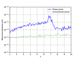
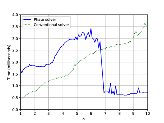
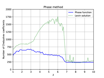
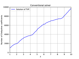
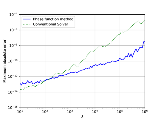
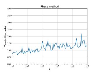
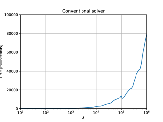
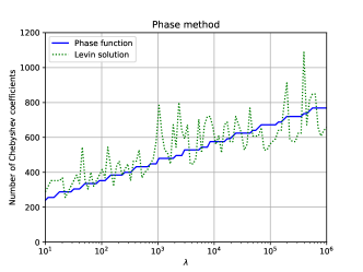
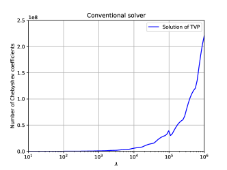
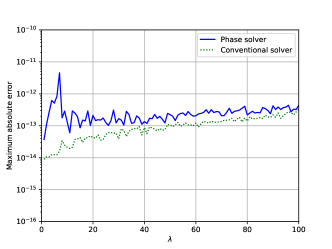
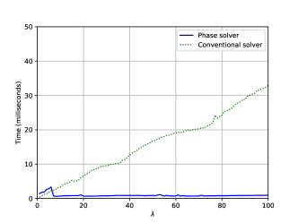
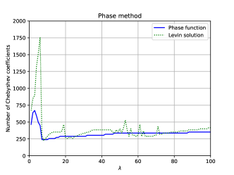
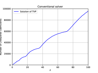
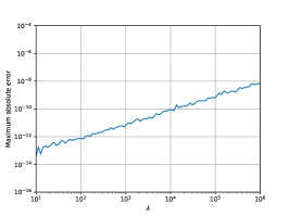
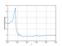
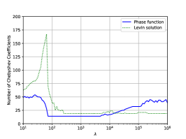
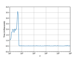
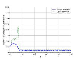
We began our first experiment by sampling $m=100$ equispaced points $x_{1},\ldots,x_{m}$ in the interval $[1,6]$. Then, for each $\lambda=10^{x_{1}},10^{x_{2}},\ldots,10^{x_{m}}$, we solved (60) using both the phase function method and the conventional solver. The wall clock time required by each method was measured, as was the number of coefficients in the piecewise Chebyshev expansion used to represent the phase function and the total number of Chebyshev coefficients in the expansions of the functions $p_{1},\ldots,p_{m}$ produced by the algorithm of Subsection 3.3. In a mild abuse of terminology, we refer to this latter quantity in the rest of this section and in our figures as the number of piecewise Chebyshev coefficients needed to represent the Levin solution. Each of the two obtained solutions was then evaluated at $10,000$ equispaced points in the interval $(-10,0)$ and the largest observed absolute errors recorded. The errors were, of course, measured by comparison with the known solution (61). We measured absolute errors rather than relative errors because (61) is an oscillatory function with many zeros on the interval $(-10,0)$. The results are presented in Figure 1. The plot at the top of that figure gives the maximum observed absolute errors in the solutions obtained by the phase function method and the conventional solver as functions of $\lambda$. The plot on the left-hand side of the second row gives the time required by the phase method as a function of $\lambda$, while the plot on the right-hand side of the second row gives the time required by the conventional solver as a function of $\lambda$. The plot on the left-hand side of the third row gives the number of coefficients in the piecewise Chebyshev expansions of the phase function and the Levin solution. The plot on the right-hand side of the third row gives the number of coefficients in the piecewise Chebyshev expansion of the solution of (60) produced by the conventional solver.

Two more experiments concerning the problem (60) were performed to test the behavior of the algorithm of this paper in the case of small values of $\lambda$. In the first of these experiments, we sampled $m=100$ equispaced points $\lambda_{1},\lambda_{2},\ldots,\lambda_{m}$ in the interval $[1,100]$. For each obtained value of $\lambda$, we repeated the procedure described above. The results are given in Figure 2. In the second of these experiments, we sampled $m=100$ equispaced points $\lambda_{1},\lambda_{2},\ldots,\lambda_{m}$ in the interval $[1,10]$ and repeated the experiments described above for each obtained value of $\lambda$. The results are shown in Figure 3.

4.2 An initial value problem

In our next experiment, we solved the initial value problem

$$\left\{\begin{aligned} &y^{\prime\prime}(t)+\left(\frac{\lambda^{2}}{0.01+t^{2}}\right)y(t)=\lambda^{2}(1+t)\cos(13t^{2}),\ \ \ 0<t<1,\\ &y(0)=y^{\prime}(0)=1.\end{aligned}\right.$$ (63)

for various values of $\lambda$ using the phase function method. More explicitly, we first sampled $m=100$ points $x_{1},x_{2},\ldots,x_{m}$ in the interval $[1,6]$. Then, for each $\lambda=10^{x_{1}},10^{x_{2}},\ldots,10^{x_{m}}$, we used the algorithm of this paper to solve (63). For each $\lambda$, we recorded the wall clock time spent solving the problem and measured the error in the obtained solution at $10,000$ equispaced points in the interval $[0,1]$. The reference solution was obtained by solving (63) using the conventional solver running in quadruple precision (REAL*16) arithmetic. The results are presented in Figure 4.

Figure 4: The results of the experiments of Subsection 4.2. The plot on the left gives the maximum observed absolute error as a function of $\lambda$; the middle plot gives the wall clock time required to solve (63) as a function of $\lambda$; and the plot on the right-hand side gives the number of coefficients in the piecewise Chebyshev expansions of the phase function and the Levin solution as functions of the parameter $\lambda$.

4.3 A boundary value problem

In the experiment described in this subsection, we solved the boundary value problem

$$\left\{\begin{aligned} &y^{\prime\prime}(t)+\left(\frac{\lambda^{3}\left(\frac{3}{2}+\cos\left(\log(\lambda)t\right)\right)}{1+\lambda\exp(t)}\right)y(t)=\frac{\lambda^{2}}{\sqrt{2+t}},\ \ \ -1<t<1,\\ &y(-1)=y(1)=0\end{aligned}\right.$$ (64)

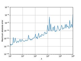
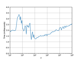
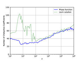
for various values of $\lambda$. More explicitly, we first sampled $m=100$ points $x_{1},x_{2},\ldots,x_{m}$ in the interval $[1,6]$. Then, for each $\lambda=10^{x_{1}},10^{x_{2}},\ldots,10^{x_{m}}$, we used the algorithm of this paper to solve (64). For each $\lambda$, we recorded the wall clock time spent solving the problem and measured the error in the obtained solution at $10,000$ equispaced points in the interval $[-1,1]$. The reference solution was obtained by solving (64) using the conventional solver running in quadruple precision (REAL*16) arithmetic. The results are presented in Figure 5. We note that the coefficient in the differential equation appearing in (64) becomes more oscillatory with $\lambda$, so we expect the running time of our algorithm to grow with $\lambda$. And while this is, in fact, the case, the effect is remarkably mild.

Figure 5: The results of the experiments of Subsection 4.3. The plot on the left gives the maximum observed absolute error as a function of $\lambda$; the middle plot gives the wall clock time required to solve (64) as a function of $\lambda$; and the plot on the right-hand side gives the number of coefficients in the piecewise Chebyshev expansions of the phase function and the Levin solution as functions of the parameter $\lambda$.

4.4 A boundary value problem with more complicated boundary conditions

In a final experiment, we solved the boundary value problem

$$\left\{\begin{aligned} &y^{\prime\prime}(t)+\left(\frac{\lambda^{2}\left(2+t^{2}\cos(\lambda)\right)}{1+t^{2}}\right)y(t)=\lambda^{2}\cos(3t^{2}),\ \ \ -1<t<1,\\ &y(-1)=y(1)\\ &y^{\prime}(-1)=y^{\prime}(1)\end{aligned}\right.$$ (65)

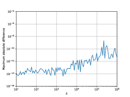
for various values of $\lambda$. We first sampled $m=100$ points $x_{1},x_{2},\ldots,x_{m}$ in the interval $[1,6]$. Then, for each $\lambda=10^{x_{1}},10^{x_{2}},\ldots,10^{x_{m}}$, we used the algorithm of this paper to solve (65). For each $\lambda$, we recorded the wall clock time spent solving the problem and measured the error in the obtained solution at $10,000$ equispaced points in the interval $[-1,1]$. The reference solution was obtained by solving (65) using the conventional solver running in quadruple precision (REAL*16) arithmetic. The results are presented in Figure 6.

Figure 6: The results of the experiments of Subsection 4.4. The plot on the left gives the maximum observed absolute error as a function of $\lambda$; the middle plot gives the wall clock time required to solve (65) as a function of $\lambda$; and the plot on the right-hand side gives the number of coefficients in the piecewise Chebyshev expansions of the phase function and the Levin solution as functions of the parameter $\lambda$.

5 Conclusions

We have introduced a scheme for solving second order inhomogeneous linear ordinary differential equations of the form

$$y^{\prime\prime}(t)+q(t)y(t)=f(t),\ \ \ \ \ a<t<b,$$ (66)

in the case in which $f$ is real-valued and slowly varying and $q$ is positive and slowly varying. Unlike standard solvers, its running time is independent of the magnitude of $q$ and, unlike asymptotic methods, the accuracy it obtains is consistent with the condition number of the problem even when $q$ is of small magnitude.

We chose the approach of this paper over another, more direct, Levin-type method precisely because we wanted an algorithm which achieves high-accuracy regardless of the magnitude of $q$. When $f$ and $q$ are slowly varying and $q$ is of sufficiently large magnitude, the equation (3) admits a nonoscillatory solution and applying an algorithm analogous to that of Subsection 2.2 to it will result in a piecewise Chebyshev expansion representing that solution. However, such an approach will fail when $q$ is of small magnitude for the reasons discussed at the end of Subsection 2.2. Nonetheless, it would be of some interest to determine when this more direct approach is preferable to the algorithm of this paper.

As mentioned in the introduction, the representation (5) of the general form of the solution of (3) is numerically unstable when $q$ is negative and of large magnitude on some or all of the interval $[a,b]$. In the authors’ view, it is unlikely that an algorithm of the type described this paper can be successfully applied to such problems in general. Nonetheless, it is most likely possible to further develop the method of this article so that it applies to important classes of physically relevant problems for which the coefficient $q$ is negative on some or all of the interval $[a,b]$ and this is the subject of ongoing work by the authors.

6 Acknowledgements

KS was supported in part by the NSERC Discovery Grants RGPIN-2020-06022 and DGECR-2020-00356. JB was supported in part by NSERC Discovery grant RGPIN-2021-02613.

Appendix A An adaptive Chebyshev spectral solver for ordinary differential equations

The algorithm of this paper entails solving several ordinary differential equations. We use a fairly standard adaptive Chebyshev spectral solver to do so. We now briefly describe its operation in the case of the initial value problem

$$\left\{\begin{aligned} \bm{y}^{\prime}(t)&=F(t,\bm{y}(t)),\ \ \ a<t<b,\\ \bm{y}(a)&=\bm{v}\end{aligned}\right.$$ (67)

where $F:\mathbb{R}^{n+1}\to\mathbb{R}^{n}$ is smooth and $\bm{v}\in\mathbb{R}^{n}$. The solver can be easily modified to apply to a terminal value problem.

The solver takes as input a positive integer $k$, a tolerance parameter $\epsilon$, an interval $(a,b)$, the vector $\bm{v}$ and a subroutine for evaluating the function $F$. It outputs $n$ piecewise $k^{th}$ order Chebyshev expansions, one for each of the components $y_{i}(t)$ of the solution $\bm{y}$ of (67).

The solver maintains two lists of subintervals of $(a,b)$: one consisting of what we term “accepted subintervals” and the other of subintervals which have yet to processed. A subinterval is accepted if the solution is deemed to be adequately represented by a $k^{th}$ order Chebyhev expansion on that subinterval. Initially, the list of accepted subintervals is empty and the list of subintervals to process contains the single interval $(a,b)$ It then operates as follows until the list of subintervals to process is empty:

1. Find, in the list of subinterval to process, the interval $(c,d)$ such that $c$ is as small as possible and remove this subinterval from the list.

2. Solve the initial value problem

   $$\left\{\begin{aligned} \bm{u}^{\prime}(t)&=F(t,\bm{u}(t)),\ \ \ c<t<d,\\ \bm{u}(c)&=\bm{w}\end{aligned}\right.$$ (68)

   If $(c,d)=(a,b)$, then we take $\bm{w}=\bm{v}$. Otherwise, the value of the solution at the point $c$ has already been approximated, and we use that estimate for $\bm{w}$ in (68).

   If the problem is linear, a straightforward integral equation method (see, for instance, [6]) is used to solve (68). Otherwise, the trapezoidal method (see, for instance, [1]) is first used to produce an initial approximation $\bm{y_{0}}$ of the solution and then Newton’s method is applied to refine it. The linearized problems are solved using an integral equation method.

   In any event, the result is a set of $k^{th}$ order Chebyshev expansions

   $$u_{i}(t)\approx\sum_{j=0}^{k}\lambda_{ij}\ T_{j}\left(\frac{2}{d-c}t+\frac{c+d}{c-d}\right),\ \ \ i=1,\ldots,n,$$ (69)

   approximating the components $u_{1},\ldots,u_{n}$ of the solution of (68).

3. Compute the quantities

   $$\frac{\sqrt{\sum_{j=\lfloor k/2\rfloor+1}^{k}\lambda_{ij}^{2}}}{\sqrt{\sum_{j=0}^{k}\lambda_{ij}^{2}}},\ \ \ i=1,\ldots,n,$$ (70)

   where the $\lambda_{ij}$ are the coefficients in the expansions (69). If any of the resulting values is larger than $\epsilon$, then we split the subinterval into two halves $\left(c,\frac{c+d}{2}\right)$ and $\left(\frac{c+d}{2},d\right)$ and place them on the list of subintervals to process. Otherwise, we place the subinterval $(c,d)$ on the list of accepted subintervals.

At the conclusion of this procedure, we have $k^{th}$ order Chebyshev expansions for each component of the solution, with the list of accepted subintervals determining the partition for each expansion.

References

- [1] Ascher, U. M., and Petzold, L. R. Computer Methods for Ordinary Differential Equations and Differential-Algebraic Equations. Society for Industrial and Applied Mathematics, USA, 1998.
- [2] Bremer, J. On the numerical solution of second order differential equations in the high-frequency regime. Applied and Computational Harmonic Analysis 44 (2018), 312–349.
- [3] Bremer, J. Phase function methods for second order linear ordinary differential equations with turning points. arXiv 2209.14561 (2022).
- [4] Bremer, J., and Rokhlin, V. Improved estimates for nonoscillatory phase functions. Discrete and Continuous Dynamical Systems, Series A 36 (2016), 4101–4131.
- [5] Chen, S., Serkh, K., and Bremer, J. The adaptive Levin method. arXiv ????.????? (2022).
- [6] Greengard, L. Spectral integration and two-point boundary value problems. SIAM Journal of Numerical Analysis 28 (1991), 1071–1080.
- [7] Kummer, E. De generali quadam aequatione differentiali tertti ordinis. Progr. Evang. Köngil. Stadtgymnasium Liegnitz (1834).
- [8] Levin, D. Procedures for computing one- and two-dimensional integrals of functions with rapid irregular oscillations. Mathematics of Computation 38 (1982), 531–5538.
- [9] Li, J., Wang, X., and Wang, T. A universal solution to one-dimensional oscillatory integrals. Science in China Series F: Information Sciences 51 (2008), 1614–1622.
- [10] Li, J., Wang, X., Wang, T., and Xiao, S. An improved Levin quadrature method for highly oscillatory integrals. Applied Numerical Mathematics 60, 8 (2010), 833–842.
- [11] Miller, P. D. Applied Asymptotic Analysis. American Mathematical Society, 2006.
- [12] Olver, F. W. Asymptotics and Special Functions. A.K. Peters, 1997.
- [13] Spigler, R. Asymptotic-numerical approximations for highly oscillatory second-order differential equations by the phase function method. Journal of Mathematical Analysis and Applications 463 (2018), 318–344.
- [14] Spigler, R., and Vianello, M. A numerical method for evaluating the zeros of solutions of second-order linear differential equations. Mathematics of Computation 55 (1990), 591–612.
- [15] Spigler, R., and Vianello, M. The phase function method to solve second-order asymptotically polynomial differential equations. Numerische Mathematik 121 (2012), 565–586.