On Pitfalls of Measuring Occlusion
Robustness through Data Distortion

Abstract

Over the past years, the crucial role of data has largely been shadowed by the field’s focus on architectures and training procedures. We often cause changes to the data without being aware of their wider implications. In this paper we show that distorting images without accounting for the artefacts introduced leads to biased results when establishing occlusion robustness. To ensure models behave as expected in real-world scenarios, we need to rule out the impact added artefacts have on evaluation. We propose a new approach, iOcclusion, as a fairer alternative for applications where the possible occluders are unknown.

1 Introduction

Correctly assessing the ability of a model to perform despite input alterations is crucial for obtaining reliable systems. Despite their incontestable success in a number of visual tasks, deep models are not fully trusted for real-world applications because of their sensitivity to input changes. This is an active area of research and proposed solutions are both at a data (DeVries & Taylor, 2017; Yun et al., 2019) as well as algorithm (Globerson & Roweis, 2006; Kortylewski et al., 2020; Zhu et al., 2019; Xu et al., 2020) level. A widely adopted method for measuring occlusion robustness is through the accuracy obtained after superimposing a rectangular patch on an image (Chun et al., 2020; Yun et al., 2019; Fawzi & Frossard, 2016; Yun et al., 2019; Zhong et al., 2020; Kokhlikyan et al., 2020). In this paper, we refer to this approach as CutOcclusion due to its similarity to the CutOut augmentation (DeVries & Taylor, 2017) and argue it can be misleading, especially in comparative studies and applications where there is no prior knowledge about the exact shape of the possible occluders. Subsequently, to address the unfairness observed, we introduce iOcclusion, a measure that could form the baseline for future robustness studies.

2 Is occlusion robustness measured fairly?

To verify the existence of the aforementioned bias, we need to compare models with different behaviours. To do this in a controlled manner, we make use of data augmentation. We focus on two popular mixed-sample augmentations, MixUp (Zhang et al., 2017b) and CutMix (Yun et al., 2019). MixUp linearly interpolates between two images to obtain a new training example, while CutMix superimposes onto a sample a rectangular region taken from another image. We also use FMix due to its irregularly shaped masks sampled from Fourier space, which will play an important role in our analysis. See Section A of the Supplementary Material for samples obtained with each method. We train PreAct-ResNet18 (He et al., 2016) and VGG (Simonyan & Zisserman, 2014) models on CIFAR-10/100 (Krizhevsky et al., 2009), FashionMNIST (Xiao et al., 2017) with these above augmentations. See Section B for experimental details.

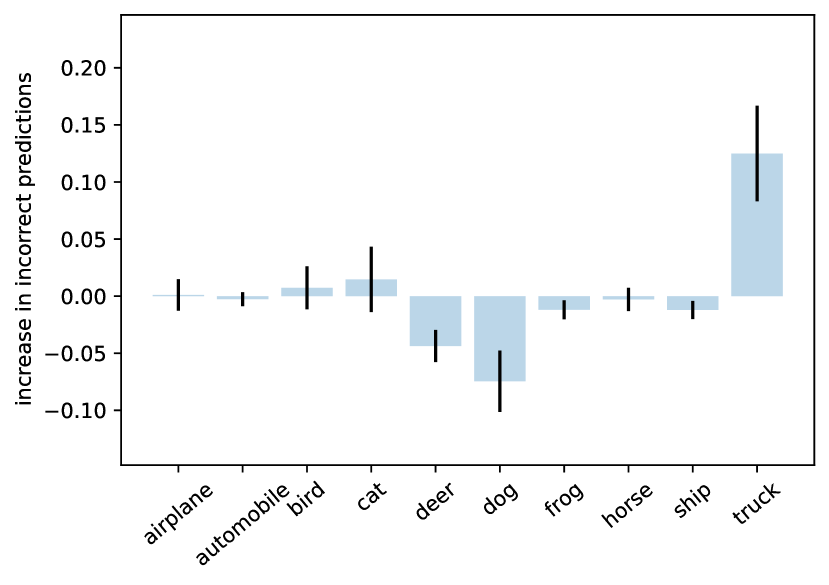
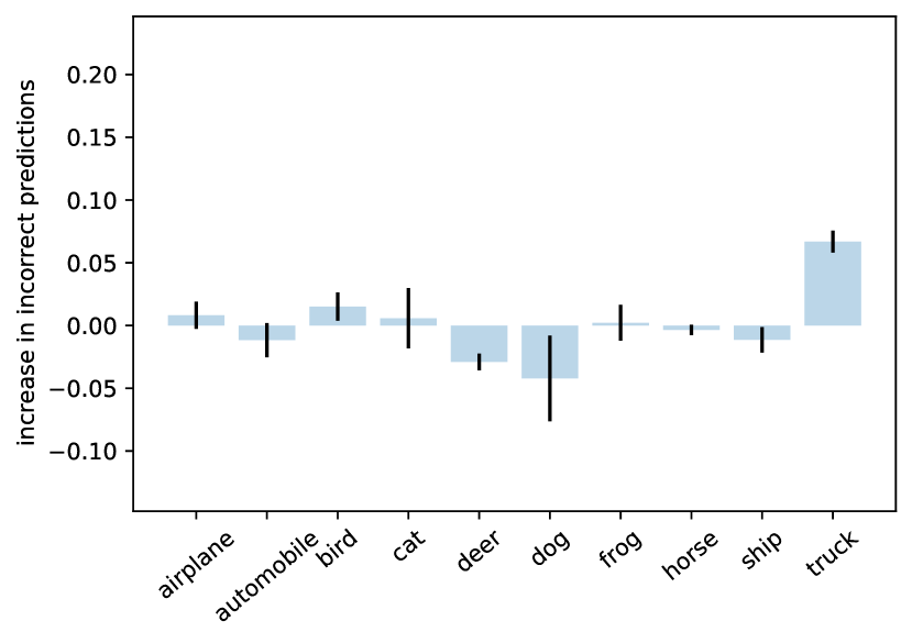
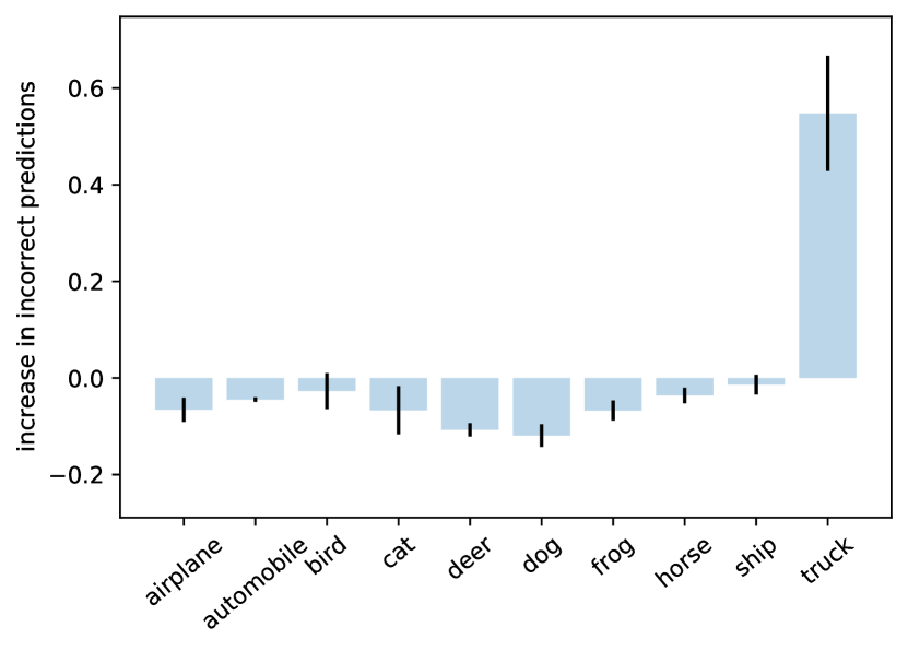
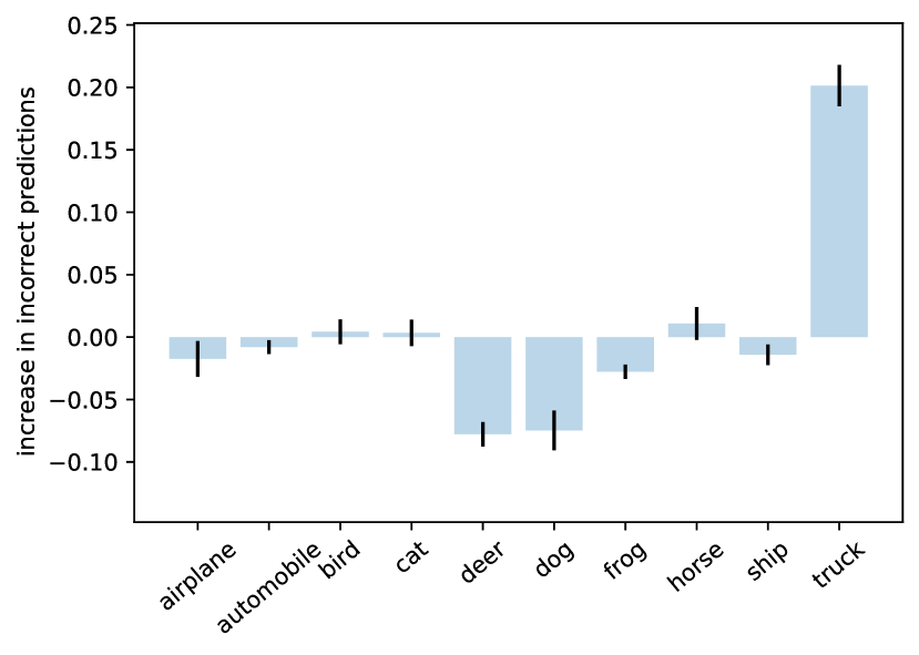
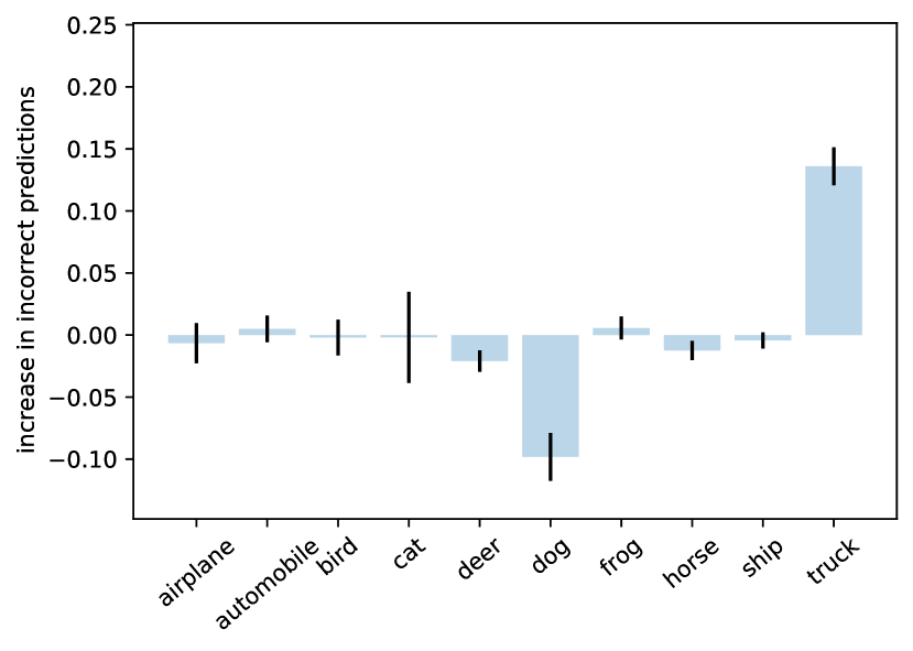
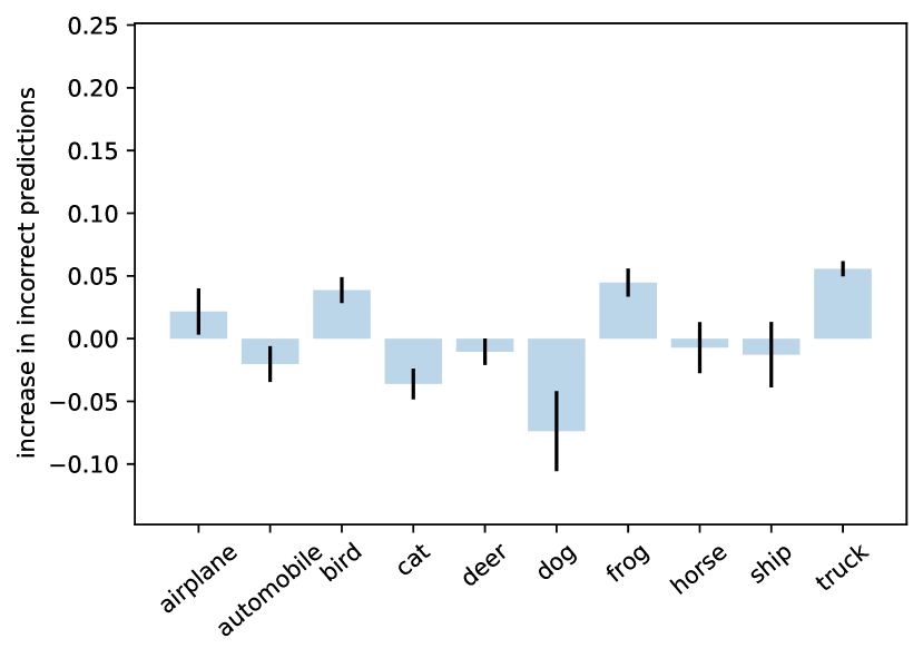
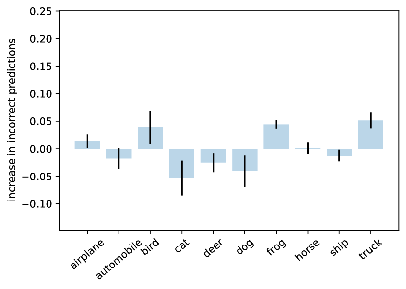
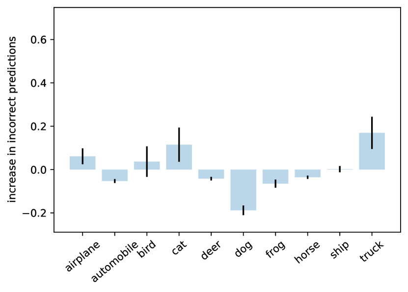
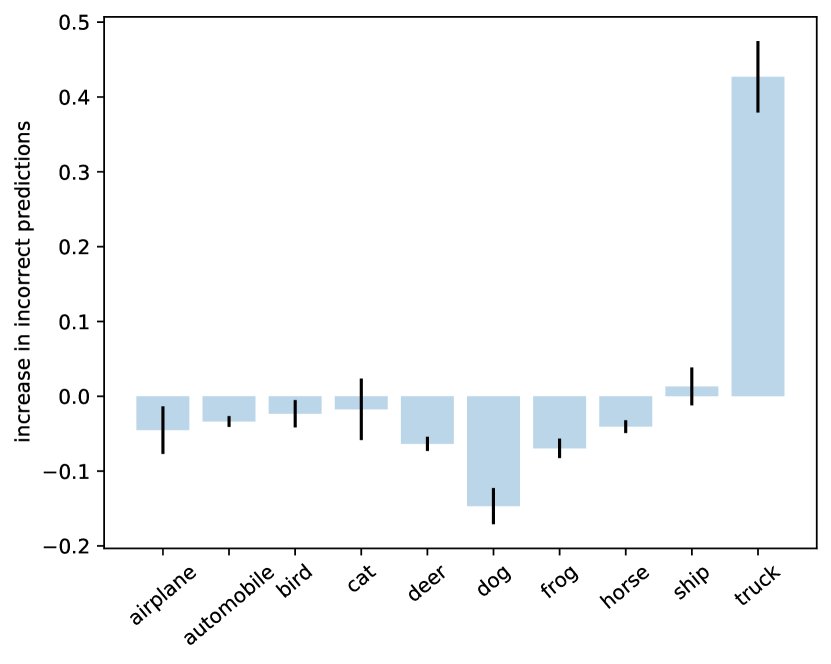
For the four types of models (basic, MixUp, FMix and CutMix) we look at the increase in misclassifications per category, when presented with CutOccluded images. That is, from the number of incorrect predictions of a model evaluated on modified data, we subtract the incorrect predictions when testing on original data. If one of the classes has a significant increase, this indicates that the distortion introduces features the model associates with that class. For all data sets, the basic model tends to wrongly predict a specific class, while between the augmented models at least one is invariant to this distortion. For example, on CIFAR-10, the basic and MixUp models tend to misclassify CutOccluded images as “Truck” (Figure 2). This is not at all surprising, given that the strong horizontal and vertical edges are highly indicative of this class. Section C contains more examples.

Admittedly, this experiment is not meant to provide a rigorous account of the bias and a comparison between the precise extent of the bias identified in various models is not possible at this stage. Nonetheless, it is sufficient to capture the broad phenomenon. Thus, by occluding images using a particularly shaped patch one implicitly measures a model’s affinity to certain features, albeit those features might be discriminative. This deems such a method inappropriate for fairly assessing robustness. Moreover, we identify similar issues in the case of texture bias identification and augmentation analyses. In the interest of space, we omit the results from the current paper, but believe this observation calls for more principled uses of data distortion in model evaluation.

A related observation was made independently of us by Hooker et al. (2019) who note the pitfalls of image manipulation in the context of interpretability methods. They focus on the distributional shift induced when removing image regions to determine feature importance. That is, they point out that when simply superimposing uniform patches over image features, it is difficult to asses how much of the reduction in accuracy is caused by the absence of those features and how much is due to images becoming out of distribution. To address this, the most important features both on train and test data are masked out, closing the gap between the two sets. They then train and respectively evaluate models on the newly generated images. Here we study a similar problem. We are interested in ruling out the overlap between the model’s learned representations and the information that is introduced by the robustness measurement method. Unlike for interpretability methods, the subject of occlusion studies is the model itself and, as such, training with a modified version of the data is not a viable option. In the following section we explore ways of overcoming this bias when measuring occlusion robustness.

2.1 iOcclusion

Figure 1: Difference in incorrect predictions for the basic model on CutOccluded images.

Figure 2: Occlusion robustness for varying fractions of image obstruction as measured with iOcclusion for the four types of models trained on CIFAR-10.

We propose a simple measure that aims to decouple the machine’s edge bias from the occlusion robustness, which we refer to as “invariant Occlusion” (iOcclusion). Invariant Occlusion reflects the change in the interplay between performance on seen and unseen data. Formally,

$$iOcclusion_{i}=\left|\frac{\mathcal{A}{(\mathcal{D}^{i}_{train})}-\mathcal{A}{(\mathcal{D}^{i}_{test})}}{\mathcal{A}{(\mathcal{D}_{train})}-\mathcal{A}{(\mathcal{D}_{test})}}\right|,$$ (1)

where $\mathcal{A}(\mathcal{D})$ denotes the accuracy on a given data set $\mathcal{D}$, and $\mathcal{D}^{i}$ is the data set resulting from removing $i\%$ pixels of each image. The intuition is that on train data robust models are less sensitive to the artefacts of the occlusion policy for small levels of occlusion, resulting in a large difference in accuracy from that on unseen data. The performance of both train and test gets close to random as the percentage of sample occlusion approaches 90% and we expect the gap to fall off quicker for less robust models. This change in interplay is taken with respect to the generalisation gap of the model. Thus, the denominator plays a normalisation role such that the quality of the model fit in itself does not interfere with the robustness measure. In this paper we choose to generate masks using Grad-CAM (Selvaraju et al., 2017), such that the area with most salient i% pixels is covered. It must be noted that this method implicitly assumes there could be multiple occluders. We also experiment with using rectangular or Fourier-sampled masks and conclude that although random masking makes the process noisier, the exact choice of masking method is of secondary importance.

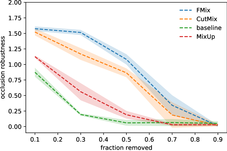
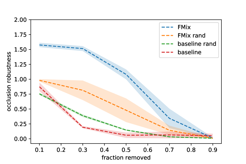
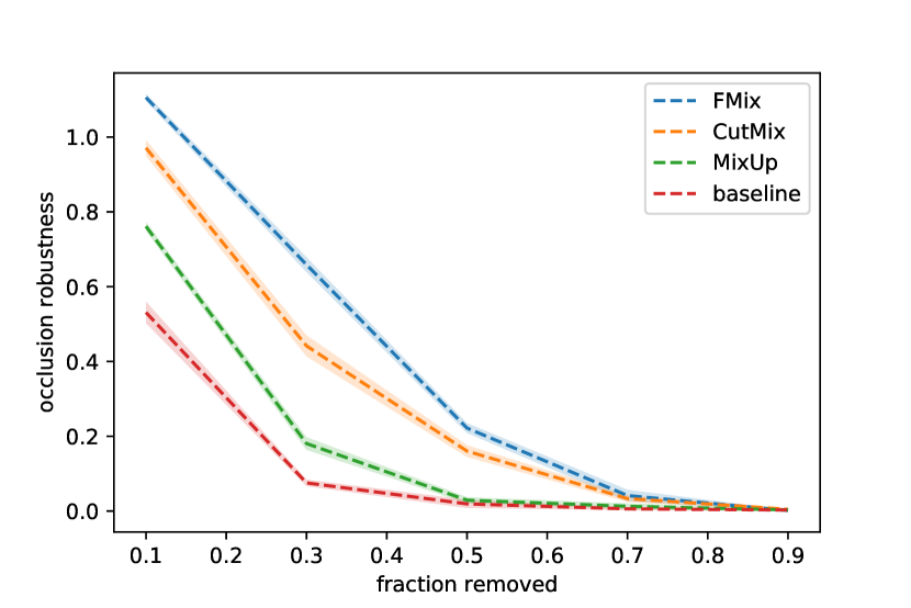
In Figure 2, we evaluate the robusteness using our method. Note that unlike the typical measure, iOcclusion is not necessarily a proper fraction. The higher robustness of FMix over CutMix is justified through the sparsity of FMix masking, as well as the way the two determine the size of the occluding patch. Although they sample the size from the same distribution, in CutMix part of the rectangle can be outside the image, which results in less occluded images overall. Thus, we will generally use the basic and FMix models as reference for least and most robust respectively.

2.2 Evaluation

Table 1: iOcclusion and CutOcclusion at a 30% obstruction level. Note that there is a difference in scale and the two should not be directly compared. We are interested in how the methods situate the models with respect to each other. When measuring the robustness with CutOcclusion, RM3 appears significantly less robust than CutMix due to its sensitivity to patching with rectangles, while iOcclusion highlights the robustness specific to FMix-like masks.

	basic	MixUp	CutMix	FMix	RM	RM3
CutOcclusion	$40.59_{\pm 2.27}$	$52.64_{\pm 1.77}$	$82.43_{\pm 1.60}$	$82.67_{\pm 0.29}$	$53.50_{4.76}$	$66.43_{\pm 6.33}$
iOcclusion	$0.19_{\pm 0.01}$	$0.56_{\pm 0.13}$	$1.16_{\pm 0.09}$	$1.51_{\pm 0.04}$	$0.63_{\pm 0.29}$	$1.45_{\pm 0.19}$

Assessing the correctness of such a measure is difficult in the absence of a basic. For the rest of this section we will build varied experiments to attest the validity of our method. We being by empirically confirming iOcclusion rules out the edge bias in CutOcclusion. We would like to train with an augmentation that has irregularly shaped masks, but at the same time doesn’t have the variation of FMix, which causes it to be insensitive to CutMix’s edges. To this end, we create two variations of FMix with which we train: RM (Random Mask) — where a single mask is sampled for the entire training; and RM3 — where for each batch one of three fixed masks is chosen uniformly at random. As for all our experiments, we do 5 repeats, for each one sampling different fixed masks. As desired, unlike FMix and CutMix, the models trained with the fixed-mask augmentation versions are highly sensitive to the edge artefacts of CutOcclusion (see Section C). Note that to allow a fairer comparison to other methods, for CutOcclusion we do not allow the obstructing patch to lie outside the image such that the fraction removed is exact. The results in Table 1 are obtained for a fraction of 0.3 pixels removed. Our measure reflects the robustness of training with three fixed random masks (RM3), situating it closer to masking methods rather than interpolative. Furthermore, iOcclusion captures the large variance in training with a fixed random mask, which shows they can range from providing almost masking-MSDA robustness to worse than MixUp.

Additionally, since occlusion in real-life scenarios could also be caused by objects that have a texture of their own, an appropriate measure must not be sensitive to the occluder’s pattern. We verify this by superimposing patches from images belonging to a different data set. For this, we perform the same operation on input as mixed-sample masking MSDAs, where the mask is given by Grad-CAM. We choose to mask with images from different data sets to avoid the side-effects of samples belonging to two classes simultaneously. The randomness introduced by the texture is naturally making the the process noisier. Nonetheless, we find again iOcclusion to better rule out the specifics of the occluding patch, whereas CutOcclusion provides significantly different results to its uniform version, pushing everything together (see Section E of the Supplementary Material).

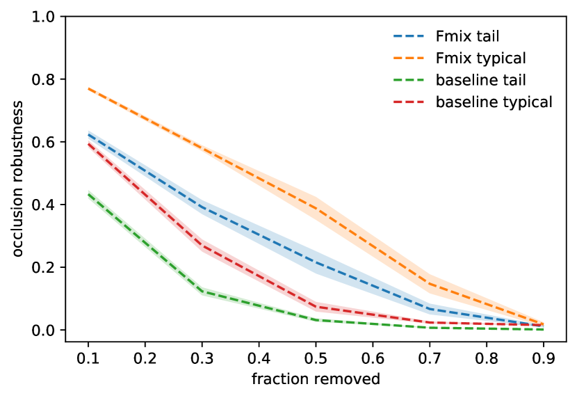
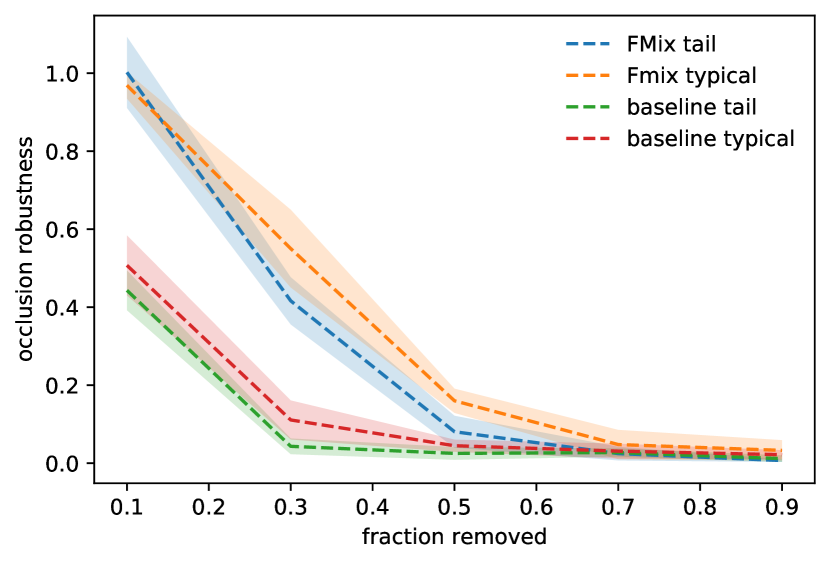
Another problem that occurs when purely looking at post-masking accuracy is weaker models would erroneously appear less robust. We show this by reversing the problem: we evaluate the same model on two subsets of the CIFAR-100 data set: typical and atypical images as categorised by Feldman & Zhang (2020). Each tail example from the train set has a corresponding one in the test set. CutOcclusion would indicate that models are significantly more robust to occluding typical examples (see Figure 3). However, a closer analysis makes us doubt this conclusion. The raw accuracy on both train and test data for tail examples is lower than for the typical ones and the decrease in performance when masking out image regions is the same for the two subsets. By definition, iOcclusion allows a fair comparison of robustness regardless of the overall performance of a model.

Figure 3: CutOcclusion (left) and iOcclusion (right) for the basic and FMix models on two subsets of the same data set, which we refer to as tail and typical. Evaluating the models with iOcclusion on the two types of samples leads robustness levels that do not differ outside the margin of error. However, CutOcclusion finds the models to be less robust on tail data.

Table 2: Robustness to occluding with patches covering $50\%$ of each image (for a full range of percentages, see Section F). The models are trained with and without masking augmentation on data with randomised labels. CutOcclusion makes no difference between regular and augmented training.

	basic random	FMix random	FMix clean
CutOcclusion	$10.24_{\pm 0.27}$	$9.78_{\pm 0.18}$	$63.63_{\pm 4.54}$
iOcclusion	$14.63_{\pm 1.12}$	$47.94_{\pm 19.84}$	$82.36_{\pm 10.06}$

Lastly, we train models on CIFAR-10 with randomly assigned labels as is done in Zhang et al. (2017a) with and without FMix, until examples are memorised. Since all labels are corrupted, the accuracy on the test set before and after occlusion is no greater than random. However, the robustness of the augmentation-trained model can be seen on the training data, as captured by our metric. On the other hand, CutOcclusion makes no distinction between learning with regular and augmented data (Table 2). Despite being such a peculiar case, it shows the comprehensiveness gained by accounting for the degradation on test data in relation to that on train.

Thus, as we evidenced through controlled experiments, there are many cases that CutOcclusion does not properly address. From a model analysis perspective, correctly assessing the occlusion robustness could lead to better understanding and development of models and training procedure. Equally important, it has applicability for real-world deployments where no prior knowledge exists about the possible shapes of the obstructions. The strength of the bias will depend on the data in question. Thus, some applications will be more heavily affected than others. However, we have seen that for natural images as is the case for CIFAR-10 and CIFAR-100 or ImageNet (Russakovsky et al., 2015), this bias does exist. We believe the edge artefacts are very likely to interfere with learned representations since they are such fundamental features. Thus, accounting for the bias is necessary to ensure a correct robustness assessment.

3 Conclusions

Distorting data without investigating its broader effects is particularly problematic when applied in analyses, as is the case of occlusion robustness measurement. We show the typical approach, CutOcclusion, is biased. This deems it inappropriate for evaluating models for real-world applications, where there is a variety of possible occluding objects. We propose iOcclusion as a basic for future robustness studies and design a number of experiments to validate it. In a broader sense, the purpose of our paper is to encourage better practice when dealing with data distortions.

Supplementary Material

Appendix A Augmentation examples

Figure 4 provides examples of new samples obtained with MixUp, CutMix, and FMix. For each pair of images, we sample a mixing coefficient $\lambda\thicksim$ Beta(1, 1) for all three augmentations. For a large value of $\lambda$, as is the case in the first column, it can be seen that CutMix covers less of Image 1 one than FMix. As mentioned in the main body of the paper, this is because CutMix allows the masking patch to lay outside of the image.

Image 1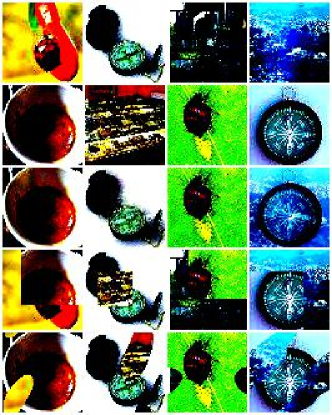
Image 2
MixUp
CutMix
FMix

Figure 4: New samples generated by the mixed-augmentations we use in our analyses.

Appendix B Experimental details

Throughout the paper, we use PreAct-ResNet18 (He et al., 2016) models, trained for 200 epochs with a batch size of 128. For the MSDA parameters we use the same values as Harris et al. (2020). All models are augmented with random crop and horizontal flip and are averaged across 5 runs. We optimise using SGD with 0.9 momentum, learning rate of 0.1 up until epoch 100 and 0.001 for the rest of the training. This is due to an incompatibility with newer versions of the PyTorch library of the official implementation of Harris et al. (2020), which we use as a starting point. However, the difference in learning rate schedule between our work and prior art does not affect our findings since we are not introducing a new method to be applied at training time. In our case, it is sufficient to show that the bias exists in at least one configuration. The models were trained on either one of the following: Titan X Pascal, GeForce GTX 1080ti or Tesla V100. For the analysis, a GeForce GTX 1050 was also used.

Training models

The code for model training is largely based on the open-source official implementation of FMix, which also includes those of MixUp, CutOut, and CutMix. For the experiment where we use the reformulated objective to combine data sets, instead of mixing with a permutation of the batch, as it is done in the original implementation of the mixed-augmentations, we now draw a batch form the desired data set. To ensure a fair comparison, for the basic we also perform inter-batch mixing.

Evaluating robustness

For the CutOcclusion measurement, we modify open-source code to restrict the occluding patch to lie withing the the margins of the image to be occluded. This is to ensure that the mixing factor $\lambda$ matches the true proportion of the occlusion. For iOcclusion, the implementation of Grad-CAM is again adapted from publicly available code. With both methods, we evaluate 5 instances of the same model and average over the results obtained.

The added computation time of iOcclusion over the regular CutOcclusion for a fixed occlusion fraction is that of performing Grad-CAM on train and test data, as well as evaluating on the latter. With a batch size of 128, this takes under half an hour.

Appendix C Analysis of wrong predictions

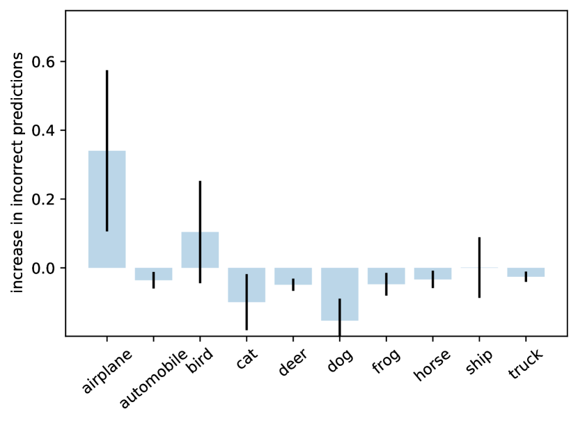
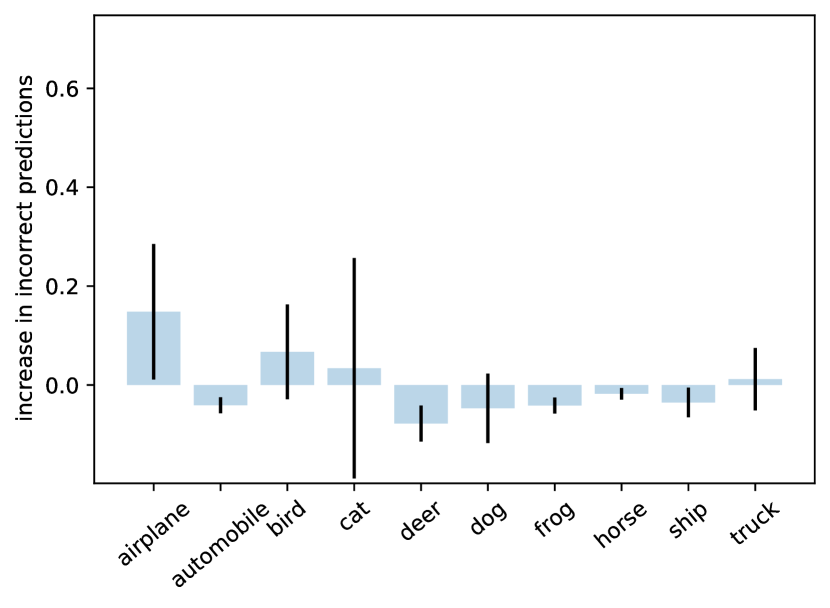
This section provides visual results of the experiments carried out to identify whether CutOcclusion provides biased results. We reintroduce the experiment here. For each class, when presented with regular test data, we count the number of times a sample was incorrectly identified as belonging to that class. We subtract the obtained values from the number of misidentifications on distorted data. Figure 6 shows results for the CIFAR-10 data set when occluding with uniform patches, while Figure 5 show results for the same problem but where occluding is done with patches corresponding to images from the CIFAR-100 data set. We mix with images from a different data set to avoid issues arising from an image belonging to two classes simultaneously. In Section G, we also show results for more data sets and architectures, while Section I contains the increase in wrong predictions obtained for the RM and RM3 models.

(a) basic

(b) MixUp

(c) CutMix

(d) FMix

Figure 5: Difference between wrongly predicted classes when testing on original data versus CutMix images. The evaluated models from left to right, top to bottom are trained on CIFAR-10 with: no mixed-data augmentation (basic), MixUp, CutMix, and FMix.

(a) basic

(b) MixUp

(c) CutMix

(d) FMix

Figure 6: Difference between wrongly predicted classes when testing on original data versus CutOut images. The evaluated models from left to right, top to bottom are trained on CIFAR-10 with: no mixed-data augmentation (basic), MixUp, CutMix, and FMix.

Appendix D Training with fixed random masks

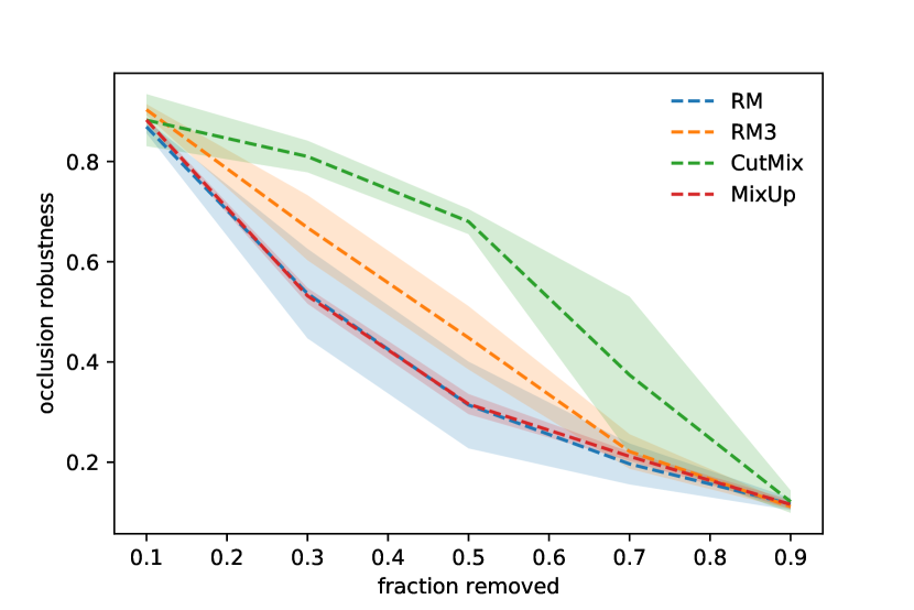
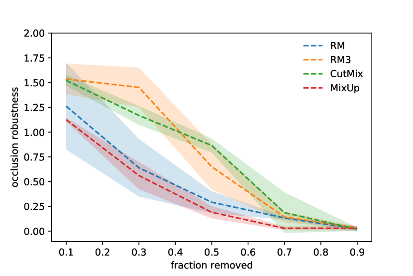
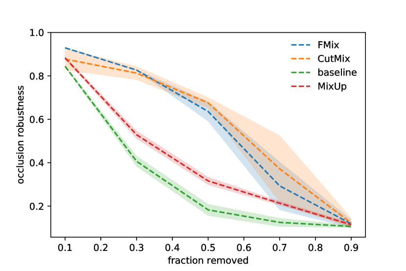
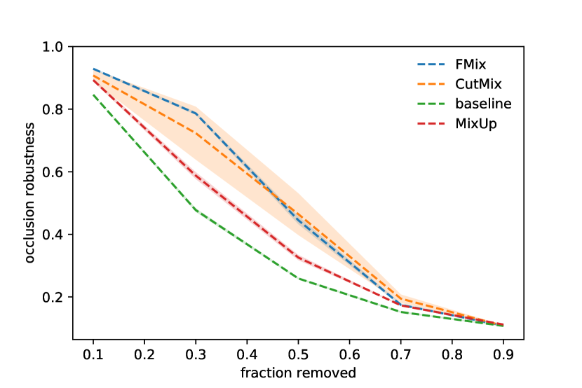
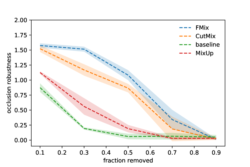
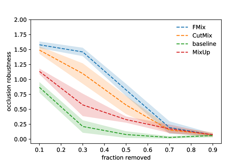
Figure 7 gives the results for CutOcclusion and iOcclusion for training with 1 or 3 random masks sampled from Fourier space. We provide CutMix and MixUp as references and exclude the basic and FMix for visual clarity.

Figure 7: CutOcclusion (left) and iOcclusion (right).

Appendix E Occluding with images from another data set

Since CutOcclusion does not account for the bias introduced by the occluding method, it is expected that changing the patch to a non-uniform one would greatly affect the results. For CIFAR-10 models, Figure 8 presents the results of occluding with CIFAR-100 images.

(a) Regular CutOcclusion

(b) Mixing CutOcclusion

(c) Regular iOcclusion

(d) Mixing iOcclusion

Figure 8: Comparison of metric sensitivity to textured occlusion. Regular occlusion refers to superimposing uniform patches over CIFAR-10 images, while mixing refers to superimposing part of CIFAR-100 samples. Mixing CutOcclusion provides significantly different results to its regular counterpart.

Appendix F Randomising labels

To assess the sensitivity of CutOcclusion and iOcclusion to the overall performance of the model, we also experiment with randomising all the labels of the CIFAR-10 data set. When evaluated on the unaugmented training data, all the basic models achieve 100% accuracy, while the FMix models reach $99.99_{\pm 0.01}$. Figure 9 gives the iOcclusion scores for these models.

Figure 9: iOcclusion results for training with clean and corrupted labels for basic and FMix augmentation.

Appendix G Distribution of wrong predictions for other data sets and architectures

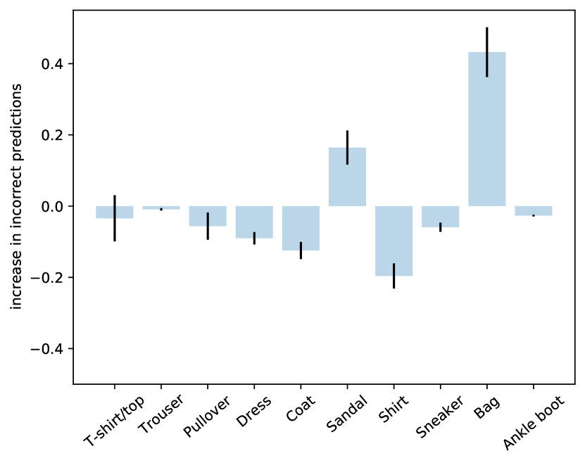
In this section we include examples of identified bias for more data sets and architectures as follows: Figure 10 for CIFAR-100, Figure 11(a) for Fashion MNIST (Xiao et al., 2017) and Figure 11(b) for VGG-16 (Simonyan & Zisserman, 2014) models. In subsequent sections of the paper we also experiment with Tiny ImageNet and ImageNet data sets, as well as BagNet models.

Figure 10: CIFAR-100 results for the basic model for CutOut images.

(a) MixUp results on Fashion MNIST. Note that for this data set, when using uniform patches, only MixUp exhibits a visible bias.

(b) Results for the basic VGG-16 model on CutOut CIFAR-10 images.

Figure 11: PreAct-ResNet18 on Fashion-MNIST (left) and VGG-16 on CIFAR-10 (right) when occluding with black patches.

Appendix H CIFAR-100 results for CutOcclusion and iOcclusion

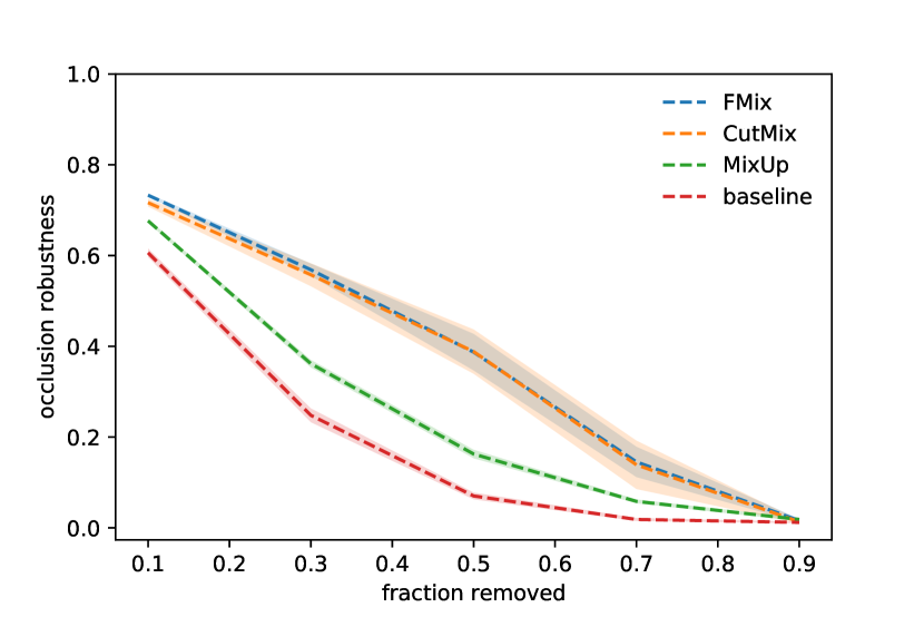
Although, as stated in the main paper, we believe it is difficult to make a direct comparison between CutOcclusion and iOcclusion, Figure 12 gives the scores for the two methods on the CIFAR-100 data set. Again, CutOcclusion only assesses the robustness against contiguous patches, making no difference between CutMix and FMix. More importantly, iOcclusion captures the more rapid fall of the masking methods, which in the case of CutOcclusion appear significantly more robust than basic due to their higher invariance to the artefacts introduced.

Figure 12: CutOcclusion (left) and iOcclusion (right) on the CIFAR-100 data set. Note again that there is a difference in scale and for comparing the two methods we look at how they position the models with respect to each other.

Appendix I Bias of fixed random masks

When training with either one or three fixed random masks sampled from Fourier space, the CIFAR-10-trained models are still predominantly predicting CutMix images as “Truck”, as depicted in Figure13. Again, the superimposed patches are taken from CIFAR-100 images.

Figure 13: Distribution of the increase in wrong predictions when evaluating on CutMix images for the model trained with one random mask (left) and three random masks (right).

References

- Chun et al. (2020) Sanghyuk Chun, Seong Joon Oh, Sangdoo Yun, Dongyoon Han, Junsuk Choe, and Youngjoon Yoo. An empirical evaluation on robustness and uncertainty of regularization methods. arXiv preprint arXiv:2003.03879, 2020.
- DeVries & Taylor (2017) Terrance DeVries and Graham W Taylor. Improved regularization of convolutional neural networks with cutout. arXiv preprint arXiv:1708.04552, 2017.
- Fawzi & Frossard (2016) Alhussein Fawzi and Pascal Frossard. Measuring the effect of nuisance variables on classifiers. In British Machine Vision Conference (BMVC), number CONF, 2016.
- Feldman & Zhang (2020) Vitaly Feldman and Chiyuan Zhang. What neural networks memorize and why: Discovering the long tail via influence estimation. Advances in Neural Information Processing Systems, 33, 2020.
- Globerson & Roweis (2006) Amir Globerson and Sam Roweis. Nightmare at test time: robust learning by feature deletion. In Proceedings of the 23rd international conference on Machine learning, pp. 353–360, 2006.
- Harris et al. (2020) Ethan Harris, Antonia Marcu, Matthew Painter, Mahesan Niranjan, Adam Prügel-Bennett, and Jonathon Hare. Understanding and enhancing mixed sample data augmentation. arXiv preprint arXiv:2002.12047, 2020.
- He et al. (2016) Kaiming He, Xiangyu Zhang, Shaoqing Ren, and Jian Sun. Identity mappings in deep residual networks. In European conference on computer vision, pp. 630–645. Springer, 2016.
- Hooker et al. (2019) Sara Hooker, Dumitru Erhan, Pieter-Jan Kindermans, and Been Kim. A benchmark for interpretability methods in deep neural networks. In Advances in Neural Information Processing Systems, pp. 9737–9748, 2019.
- Kokhlikyan et al. (2020) Narine Kokhlikyan, Vivek Miglani, Miguel Martin, Edward Wang, Bilal Alsallakh, Jonathan Reynolds, Alexander Melnikov, Natalia Kliushkina, Carlos Araya, Siqi Yan, and Orion Reblitz-Richardson. Captum: A unified and generic model interpretability library for pytorch, 2020.
- Kortylewski et al. (2020) Adam Kortylewski, Qing Liu, Angtian Wang, Yihong Sun, and Alan Yuille. Compositional convolutional neural networks: A robust and interpretable model for object recognition under occlusion. International Journal of Computer Vision, pp. 1–25, 2020.
- Krizhevsky et al. (2009) Alex Krizhevsky et al. Learning multiple layers of features from tiny images. 2009.
- Russakovsky et al. (2015) Olga Russakovsky, Jia Deng, Hao Su, Jonathan Krause, Sanjeev Satheesh, Sean Ma, Zhiheng Huang, Andrej Karpathy, Aditya Khosla, Michael Bernstein, et al. Imagenet large scale visual recognition challenge. International journal of computer vision, 115(3):211–252, 2015.
- Selvaraju et al. (2017) Ramprasaath R Selvaraju, Michael Cogswell, Abhishek Das, Ramakrishna Vedantam, Devi Parikh, and Dhruv Batra. Grad-cam: Visual explanations from deep networks via gradient-based localization. In Proceedings of the IEEE international conference on computer vision, pp. 618–626, 2017.
- Simonyan & Zisserman (2014) Karen Simonyan and Andrew Zisserman. Very deep convolutional networks for large-scale image recognition. arXiv preprint arXiv:1409.1556, 2014.
- Xiao et al. (2017) Han Xiao, Kashif Rasul, and Roland Vollgraf. Fashion-mnist: a novel image dataset for benchmarking machine learning algorithms. arXiv preprint arXiv:1708.07747, 2017.
- Xu et al. (2020) Zhenlin Xu, Deyi Liu, Junlin Yang, and Marc Niethammer. Robust and generalizable visual representation learning via random convolutions. arXiv preprint arXiv:2007.13003, 2020.
- Yun et al. (2019) Sangdoo Yun, Dongyoon Han, Seong Joon Oh, Sanghyuk Chun, Junsuk Choe, and Youngjoon Yoo. Cutmix: Regularization strategy to train strong classifiers with localizable features. In Proceedings of the IEEE International Conference on Computer Vision, pp. 6023–6032, 2019.
- Zhang et al. (2017a) Chiyuan Zhang, Samy Bengio, Moritz Hardt, Benjamin Recht, and Oriol Vinyals. Understanding deep learning requires rethinking generalization. In International Conference on Learning Representations, 2017a.
- Zhang et al. (2017b) Hongyi Zhang, Moustapha Cisse, Yann N Dauphin, and David Lopez-Paz. mixup: Beyond empirical risk minimization. arXiv preprint arXiv:1710.09412, 2017b.
- Zhong et al. (2020) Zhun Zhong, Liang Zheng, Guoliang Kang, Shaozi Li, and Yi Yang. Random erasing data augmentation. In AAAI, pp. 13001–13008, 2020.
- Zhu et al. (2019) Hongru Zhu, Peng Tang, Jeongho Park, Soojin Park, and Alan Yuille. Robustness of object recognition under extreme occlusion in humans and computational models. arXiv preprint arXiv:1905.04598, 2019.