Computational multiscale methods for nondivergence-form elliptic partial differential equations

Abstract.

This paper proposes novel computational multiscale methods for linear second-order elliptic partial differential equations in nondivergence-form with heterogeneous coefficients satisfying a Cordes condition. The construction follows the methodology of localized orthogonal decomposition (LOD) and provides operator-adapted coarse spaces by solving localized cell problems on a fine scale in the spirit of numerical homogenization. The degrees of freedom of the coarse spaces are related to nonconforming and mixed finite element methods for homogeneous problems. The rigorous error analysis of one exemplary approach shows that the favorable properties of the LOD methodology known from divergence-form PDEs, i.e., its applicability and accuracy beyond scale separation and periodicity, remain valid for problems in nondivergence-form.

1. Introduction

In this work, we consider linear second-order elliptic partial differential equations of the form

$$A:D^{2}u+b\cdot\nabla u-c\,u\coloneqq\sum_{i,j=1}^{n}a_{ij}\,\partial_{ij}^{2}u+\sum_{k=1}^{n}b_{k}\,\partial_{k}u-c\,u=f\quad\text{in }\Omega,$$ (1.1)

posed on a bounded convex polyhedral domain $\Omega\subset\mathbb{R}^{n}$, $n\geq 2$, with a right-hand side $f\in L^{2}(\Omega)$, subject to the homogeneous Dirichlet boundary condition

$$u=0\quad\text{on }\partial\Omega,$$ (1.2)

where $A=(a_{ij})_{1\leq i,j\leq n}\in L^{\infty}(\Omega;\mathbb{R}^{n\times n}_{\mathrm{sym}})$, $b=(b_{k})_{1\leq k\leq n}\in L^{\infty}(\Omega;\mathbb{R}^{n})$, and $c\in L^{\infty}(\Omega)$ are heterogeneous coefficients such that $A$ is uniformly elliptic, $c\geq 0$ almost everywhere in $\Omega$, and the triple $(A,b,c)$ satisfies a (generalized) Cordes condition. Our main objective in this paper is to propose and rigorously analyze a novel finite element scheme for the accurate numerical approximation of the solution to the multiscale problem 1.1–1.2, a task we will refer to as numerical homogenization, by following the methodology of localized orthogonal decomposition (LOD) [MaP14, MalP20]. It is worth mentioning that we are working in a framework beyond periodicity and separation of scales.

The motivation for investigating 1.1–1.2 stems from engineering, physics, and mathematical areas such as stochastic analysis. Notably, such equations arise in the linearization of Hamilton–Jacobi–Bellman (HJB) equations from stochastic control theory. A distinguishing feature of nondivergence-form problems such as 1.1–1.2 is the absence of a natural variational formulation. However, due to the Cordes condition, there exists a unique strong solution to 1.1–1.2 which can be equivalently characterized as the unique solution to the Lax–Milgram-type problem

$$\text{seek }u\in V\coloneqq H^{2}(\Omega)\cap H^{1}_{0}(\Omega)\text{ such that }a(u,v)=\langle F,v\rangle\text{ for all }v\in V$$ (1.3)

with some suitably defined $F\in V^{\ast}$ and bounded coercive bilinear form $a:V\times V\rightarrow\mathbb{R}$.

In the presence of coefficients that vary on a fine scale, e.g., when $A(x)=\tilde{A}(\frac{x}{\varepsilon})$ with some $(0,1)^{n}$-periodic $\tilde{A}\in L^{\infty}(\mathbb{R}^{n};\mathbb{R}^{n\times n}_{\mathrm{sym}})$ and $\varepsilon>0$ small, classical finite element methods are being outperformed by multiscale finite element methods such as developed in this paper. For periodic coefficients, periodic homogenization has been proposed for linear elliptic equations in nondivergence-form, cf. [AL89, BLP11, GST22, GTY20, JKO94, KL16, Spr23, ST21]. Numerical homogenization of such problems has not been studied extensively so far. A finite element numerical homogenization scheme for the periodic setting has been proposed and analyzed in [CSS20], which is based on an approximation of the solution to the homogenized problem via a finite element approximation of an invariant measure (see also [Spr23]). Further, there has been some previous study on finite difference approaches for such problems in the periodic setting; see [AK18, FO09]. Concerning fully-nonlinear HJB and Isaacs equations, finite element approaches for the numerical homogenization in the periodic setting have been suggested in [GSS21, KS22] and some finite difference schemes have been studied in [CM09, FO18, FOO18].

The case of arbitrarily rough coefficients beyond periodicity and scale separation has not yet been addressed. For divergence-form PDEs, several numerical homogenization methods have been developed in the last decade, which are based on the construction of operator-adapted basis functions and are applicable without such structural assumptions. We highlight the LOD [MaP14, HeP13, KPY18, Mai20], the Generalized Finite Element Method [BaL11, EGH13, Ma22], Rough Polyharmonic Splines and Gamblets [OZB14, Owh17] as well as the recently proposed Super-Localized Orthogonal Decomposition [HP21pre, FHP21, BFP22].

The aim of this paper is to transfer such modern numerical homogenization methods to the case of nondivergence-form problems, and to provide a proof of concept that this framework also applies to this class of equations. The only existing link between numerical homogenization and nondivergence-form problems is the metric-based upscaling proposed in [OZ07] which exploits nondivergence-form problems for a problem-dependent change of metric as part of the numerical homogenization of divergence-form problems. Our construction of a practical finite element method for the nondivergence-form problem 1.1–1.2 in the presence of multiscale data follows the abstract LOD framework for numerical homogenization methods for divergence-form problems presented in [AHP21]. It is based on the problem 1.3 as starting point, $a$-orthogonal decompositions of the solution space $V$ and the test space $V$ into a fine-scale space – defined as the intersection of the kernels of suitably chosen quantities of interest $q_{1},\dots,q_{N}\in V^{\ast}$ – and some coarse scale space, and a localization argument. In our exemplary approach, the choice of quantities of interests is inspired by the degrees of freedom of the nonconforming Morley finite element.

The remainder of this work is organized as follows. In Section 2, we present the problem setting as well as the theoretical foundation including the well-posedness of 1.1–1.2 based on a Cordes condition. In Section 3, we introduce the numerical homogenization scheme for the approximation of the solution to 1.1–1.2 based on LOD theory. The proposed numerical homogenization scheme is rigorously analyzed and error bounds are proved. The numerical implementation is based on a $H^{2}$-conforming Birkhoff–Mansfield element and is introduced in Section 4.1. In Section 4, we illustrate the theoretical findings by several numerical experiments and finally, in LABEL:sec:Alternative_discretization_using_a_mixed_non-symmetric_FEM, we discuss an alternative discretization based on mixed finite element theory.

2. Problem setting and well-posedness

2.1. Framework

For a bounded convex polyhedral domain $\Omega\subset\mathbb{R}^{n}$ in dimension $n\geq 2$, and a right-hand side $f\in L^{2}(\Omega)$, we consider the problem

$$\left\{\begin{aligned} Lu\coloneqq A:D^{2}u+b\cdot\nabla u-c\,u&=f\quad\text{in }\Omega,\\ u&=0\quad\text{on }\partial\Omega,\end{aligned}\right.$$ (2.1)

where we assume that

$$A\in L^{\infty}(\Omega;\mathbb{R}^{n\times n}_{\mathrm{sym}}),\quad b\in L^{\infty}(\Omega;\mathbb{R}^{n}),\quad c\in L^{\infty}(\Omega)\text{ with }c\geq 0\text{ a.e. in }\Omega,$$

that $A$ is uniformly elliptic, i.e., there exist constants $\zeta_{1},\zeta_{2}>0$ such that

$$\forall\xi\in\mathbb{R}^{n}\backslash\{0\}:\quad\zeta_{1}\leq\frac{A\xi\cdot\xi}{\lvert\xi\rvert^{2}}\leq\zeta_{2}\quad\text{a.e. in }\Omega,$$ (2.2)

and that the triple $(A,b,c)$ satisfies the Cordes condition, that is, we make the following assumption:

• If $\lvert b\rvert=c=0$ a.e. in $\Omega$, we assume that there exists a constant $\delta\in(0,1)$ such that

  $$\frac{\lvert A\rvert^{2}}{(\mathrm{tr}(A))^{2}}\leq\frac{1}{n-1+\delta}\quad\text{ a.e. in }\Omega.$$ (2.3)

  Further, in this case we set $\gamma\coloneqq\frac{\mathrm{tr}(A)}{\lvert A\rvert^{2}}$ and $\lambda\coloneqq 0$.

• Otherwise, we assume that there exist constants $\delta\in(0,1)$ and $\lambda\in(0,\infty)$ such that

  $$\frac{\lvert A\rvert^{2}+\frac{1}{2\lambda}\lvert b\rvert^{2}+\frac{1}{\lambda^{2}}c^{2}}{\left(\mathrm{tr}(A)+\frac{1}{\lambda}c\right)^{2}}\leq\frac{1}{n+\delta}\quad\text{ a.e. in }\Omega.$$ (2.4)

  Further, in this case we set $\gamma\coloneqq\frac{\mathrm{tr}(A)+\frac{1}{\lambda}c}{\lvert A\rvert^{2}+\frac{1}{2\lambda}\lvert b\rvert^{2}+\frac{1}{\lambda^{2}}c^{2}}$.

Here, we have used the notation $\lvert M\rvert\coloneqq\sqrt{M:M}$ to denote the Frobenius norm of $M\in\mathbb{R}^{n\times n}$.

Remark 2.1.

When $n=2$, uniform ellipticity 2.2 guarantees that the condition 2.3 is satisfied for some $\delta\in(0,1)$; see e.g., [SS14].

Remark 2.2 (Properties of $\gamma$).

Note that $\gamma\in L^{\infty}(\Omega)$ and that there exist constants $\gamma_{0},\Gamma>0$ depending only on $n,\zeta_{1},\zeta_{2},\lambda,\|b\|_{L^{\infty}(\Omega)},\|c\|_{L^{\infty}(\Omega)}$ such that $\gamma_{0}\leq\gamma\leq\Gamma$ a.e. in $\Omega$.

2.2. Well-posedness

We introduce the Hilbert space $(V,(\cdot,\cdot)_{V})$ by setting

$$V\coloneqq H^{2}(\Omega)\cap H^{1}_{0}(\Omega),\qquad(\cdot,\cdot)_{V}\coloneqq(\cdot,\cdot)_{H^{2}(\Omega)},$$ (2.5)

and we write $\|\cdot\|_{V}\coloneqq\|\cdot\|_{H^{2}(\Omega)}$ and $\|\cdot\|_{V,\omega}\coloneqq\|\cdot\|_{H^{2}(\omega)}$ for any subdomain $\omega\subset\Omega$. Then, introducing the bilinear form

$$a:V\times V\rightarrow\mathbb{R},\qquad a(v_{1},v_{2})\coloneqq\left(\gamma\,Lv_{1},\Delta v_{2}-\lambda v_{2}\right)_{L^{2}(\Omega)},$$

the linear operator

$$\mathcal{A}:V\rightarrow V^{\ast},\qquad v\mapsto\mathcal{A}v\coloneqq a(v,\cdot),$$

and the linear functional

$$F:V\rightarrow\mathbb{R},\qquad v\mapsto\langle F,v\rangle\coloneqq\left(\gamma f,\Delta v-\lambda v\right)_{L^{2}(\Omega)},$$

it is well-known that we have existence and uniqueness of a strong solution to (2.1); see [SS13, SS14]:

Theorem 2.1 (Well-posedness).

The following assertions hold true.

• A function $u\in V$ is a strong solution to 2.1 if, and only if,

  $$a(u,v)=\langle F,v\rangle\quad\text{for all }v\in V.$$ (2.6)

• There exists a unique $u\in V$ such that $\mathcal{A}u=F$ in $V^{\ast}$, i.e., $a(u,v)=\langle F,v\rangle$ for all $v\in V$.

In particular, the problem 2.1 has a unique strong solution $u\in V$.

Note that assertion (i) of 2.1 follows immediately from the fact that for any $g\in L^{2}(\Omega)$ there exists a unique $v\in V$ such that $\Delta v-\lambda v=g$, and the positivity of the renormalization function $\gamma$. Assertion (ii) of 2.1 is shown by a standard Lax–Milgram argument using the properties of $a$ and $F$ listed below.

Lemma 2.1 (Properties of the maps $a$ and $F$).

The following assertions hold true.

• Local boundedness of $a$: There exists a constant $C_{a}>0$ depending only on $n,\zeta_{1},\zeta_{2}$, $\lambda$,$\|b\|_{L^{\infty}(\Omega)}$,$\|c\|_{L^{\infty}(\Omega)}$ such that for any subdomains $\omega_{1},\omega_{2}\subset\Omega$ we have that

  $$\forall v_{1},v_{2}\in V:\quad\mathrm{supp}(v_{1})\subset\omega_{1},\mathrm{supp}(v_{2})\subset\omega_{2}\quad\Longrightarrow\quad\lvert a(v_{1},v_{2})\rvert\leq C_{a}\|v_{1}\|_{V,\omega_{1}\cap\omega_{2}}\|v_{2}\|_{V,\omega_{1}\cap\omega_{2}}.$$

• Coercivity of $a$: There exists a constant $\alpha>0$ depending only on $\mathrm{diam}(\Omega),n,\delta$ such that

  $$a(v,v)\geq(1-\sqrt{1-\delta})\|\Delta v-\lambda v\|_{L^{2}(\Omega)}^{2}\geq\alpha\|v\|_{V}^{2}\qquad\forall v\in V.$$

• $F\in V^{*}$: There exists a constant $\mu>0$ depending only on $n,\zeta_{1},\zeta_{2},\lambda,\|b\|_{L^{\infty}(\Omega)},\|c\|_{L^{\infty}(\Omega)}$ such that

  $$\lvert\langle F,v\rangle\rvert\leq\mu\|f\|_{L^{2}(\Omega)}\|v\|_{V}\qquad\forall v\in V,$$

  or equivalently, $\|F\|_{V^{*}}\leq\mu\|f\|_{L^{2}(\Omega)}$.

The proofs of assertions (i) and (iii) of 2.1 are straightforward. A proof of assertion (ii) of 2.1 can be found in [SS13, SS14], relying on the observation that the Cordes condition implies that for any subdomain $\omega\subset\Omega$ we have that (see Lemma 1 in [SS14])

$$\forall v\in H^{2}(\omega):\qquad\lvert\gamma\,Lv-(\Delta v-\lambda v)\rvert\leq\sqrt{1-\delta}\sqrt{\lvert D^{2}v\rvert^{2}+2\lambda\lvert\nabla v\rvert^{2}+\lambda^{2}v^{2}}\quad\text{a.e. in }\omega,$$

and using the Miranda–Talenti-type estimates (see Theorem 2 in [SS14])

$$\|D^{2}v\|_{L^{2}(\Omega)}^{2}+2\lambda\|\nabla v\|_{L^{2}(\Omega)}^{2}+\lambda^{2}\|v\|_{L^{2}(\Omega)}^{2} \leq\|\Delta v-\lambda v\|_{L^{2}(\Omega)}^{2}\qquad\quad\;\;\;\forall v\in V,$$

$$\|v\|_{V} \leq C_{\mathrm{MT}}\|\Delta v-\lambda v\|_{L^{2}(\Omega)}\qquad\forall v\in V,$$

with a constant $C_{\mathrm{MT}}>0$ depending only on $\mathrm{diam}(\Omega)$ and $n$.

Remark 2.3.

In view of 2.1 and 2.1, the unique strong solution $u\in V$ to 2.1 satisfies the bound

$$\|u\|_{V}\leq\alpha^{-1}\|F\|_{V^{*}}\leq\alpha^{-1}\mu\|f\|_{L^{2}(\Omega)},$$

where $\alpha,\mu>0$ are the constants from 2.1(ii)–(iii).

It is worth emphasizing that in the setting of periodic homogenization, i.e., $A=\tilde{A}(\frac{\cdot}{\varepsilon})$, $b=\tilde{b}(\frac{\cdot}{\varepsilon})$, $c=\tilde{c}(\frac{\cdot}{\varepsilon})$ for some small parameter $\varepsilon>0$ and $(0,1)^{n}$-periodic $\tilde{A},\tilde{b},\tilde{c}\in L^{\infty}(\mathbb{R}^{n})$ satisfying the Cordes condition in $\mathbb{R}^{n}$, we have that the $H^{2}(\Omega)$-norm of the solution to (2.1) is uniformly bounded in $\varepsilon\in(0,1)$, while generically the $H^{2+s}(\Omega)$-norm is unbounded as $\varepsilon\searrow 0$ for any $s>0$. Note that this is different to the usual periodic homogenization setting for divergence-form equations where generically the $H^{2}(\Omega)$-norm is unbounded as $\varepsilon\searrow 0$.

3. Numerical homogenization scheme

For simplicity, we only work in dimension $n=2$ and give some remarks on numerical homogenization in higher dimensions in LABEL:Sec:_ext_and_fw.

3.1. Fine-scale space

We start by introducing a triangulation of the bounded convex polygon $\Omega\subset\mathbb{R}^{2}$. Thereafter, we define a certain closed linear subspace $W$ of $V$ (recall the definition of $V$ from 2.5) which will be referred to as the fine-scale space.

3.1.1. Triangulation

Let $\mathcal{T}_{H}$ be a regular quasi-uniform triangulation of $\Omega$ into closed triangles with mesh-size $H>0$ and shape-regularity parameter $\rho>0$ given by

$$H\coloneqq\max_{T\in\mathcal{T}_{H}}\mathrm{diam}(T),\qquad\rho\coloneqq H^{-1}\min_{T\in\mathcal{T}_{H}}\rho_{T},$$

where $\rho_{T}$ denotes the diameter of the largest ball which can be inscribed in the element $T$. We introduce the piecewise constant mesh-size function $h_{\mathcal{T}_{H}}:\bar{\Omega}\rightarrow\mathbb{R}$ given by $\left.h_{\mathcal{T}_{H}}\right\rvert_{T}\coloneqq H_{T}\coloneqq\lvert T\rvert^{\frac{1}{2}}$ for $T\in\mathcal{T}_{H}$. Let $\mathcal{F}_{H}$ denote the set of edges, $\mathcal{N}_{H}^{\mathrm{int}}$ the set of interior vertices, $\mathcal{N}_{H}^{\partial}$ the set of boundary vertices, and define

$$N_{1}\coloneqq\lvert\mathcal{F}_{H}\rvert,\qquad N_{2}\coloneqq\lvert\mathcal{N}_{H}^{\mathrm{int}}\rvert,\qquad N\coloneqq N_{1}+N_{2}.$$

We label the edges $F_{1},\dots,F_{N_{1}}$ and the interior vertices $z_{1},\dots,z_{N_{2}}$, so that

$$\mathcal{F}_{H}=\{F_{1},F_{2},\dots,F_{N_{1}}\},\qquad\mathcal{N}_{H}^{\mathrm{int}}=\{z_{1},z_{2},\dots,z_{N_{2}}\}.$$

For each edge $F\in\mathcal{F}_{H}$ we associate a fixed choice of unit normal $\nu_{F}$, where we often drop the subscript and only write $\nu$ for simplicity. Finally, for a subset $S\subset\Omega$, we define $N^{0}(S)\coloneqq S$ and $N^{\ell}(S)\coloneqq\bigcup\{T\in\mathcal{T}_{H}:T\cap N^{\ell-1}(S)\neq\emptyset\}$ for $\ell\in\mathbb{N}$.

3.1.2. Quantities of interest and the space of fine-scale functions

First, let us note that $V\subset C(\bar{\Omega})$ by Sobolev embeddings. For $i\in\{1,\dots,N\}$, we define the quantity of interest $q_{i}\in V^{\ast}$ by

$$q_{i}:V\rightarrow\mathbb{R},\qquad v\mapsto\langle q_{i},v\rangle\coloneqq\begin{cases}\mathchoice{{\vbox{\hbox{$\textstyle-$}}\kern-4.86108pt}}{{\vbox{\hbox{$\scriptstyle-$}}\kern-3.25pt}}{{\vbox{\hbox{$\scriptscriptstyle-$}}\kern-2.29166pt}}{{\vbox{\hbox{$\scriptscriptstyle-$}}\kern-1.875pt}}\!\int_{F_{i}}\nabla v\cdot\nu&,\text{ if }1\leq i\leq N_{1},\\ v(z_{i-N_{1}})&,\text{ if }N_{1}+1\leq i\leq N.\end{cases}$$

The quantities of interest $\{q_{1},\dots,q_{N}\}\subset V^{\ast}$ are linearly independent as can be seen from the fact that there exist functions $u_{1},\dots,u_{N}\in V$ such that $\langle q_{i},u_{j}\rangle=\delta_{ij}$ for any $i,j\in\{1,\dots,N\}$; see Section 3.3.1. We define the fine-scale space

$$W\coloneqq\bigcap_{i\in\{1,\dots,N\}}\mathrm{ker}(q_{i})=\{\left.v\in V\,\right\rvert\langle q_{i},v\rangle=0\;\;\forall\,i\in\{1,\dots,N\}\},$$ (3.1)

which is a closed linear subspace of $V$.

3.1.3. Connection to the Morley finite element space

We consider the Morley finite element space

$$V_{H}^{\mathrm{Mor}}\coloneqq\{\left.v\in\mathcal{P}_{2}(\mathcal{T}_{H})\,\right\rvert v\text{ is continuous at }\mathcal{N}_{H}^{\mathrm{int}}\text{ and vanishes at }\mathcal{N}_{H}^{\partial};$$

$$D_{\mathrm{NC}}v\text{ is continuous at the interior edges' midpoints}\},$$

whose local degrees of freedom are the evaluation of the function at each vertex and the evaluation of the normal derivative at the edges’ midpoints. Here, the piecewise action of the differential operator $D$ is indicated by the subscript $\mathrm{NC}$, i.e., we define $\left.(D_{\mathrm{NC}}v)\right\rvert_{T}:=\left.D(v\right\rvert_{T})$ for any $T\in\mathcal{T}_{H}$. Then, letting $\{\phi_{1},\dots,\phi_{N}\}\subset V_{H}^{\mathrm{Mor}}$ denote Morley basis functions satisfying $\langle q_{i},\phi_{j}\rangle=\delta_{ij}$ for all $i,j\in\{1,\dots,N\}$ (note $\langle q_{i},\phi_{j}\rangle$ is well-defined although $\phi_{j}\not\in V$), we have that the Morley interpolation operator is given by

$$\Pi^{\mathrm{Mor}}:V\rightarrow V_{H}^{\mathrm{Mor}},\qquad v\mapsto\Pi^{\mathrm{Mor}}v\coloneqq\sum_{i=1}^{N}\langle q_{i},v\rangle\phi_{i},$$ (3.2)

and we observe that

$$W=\mathrm{ker}(\Pi^{\mathrm{Mor}})=\{\left.v\in V\,\right\rvert\Pi^{\mathrm{Mor}}v=0\}.$$

In particular, using Morley interpolation bounds (see e.g., [WX13]), we have the local estimate

$$\|w\|_{L^{2}(T)}+H_{T}\|\nabla w\|_{L^{2}(T)}\lesssim H_{T}^{2}\|D^{2}w\|_{L^{2}(T)}\qquad\forall T\in\mathcal{T}_{H}\quad\forall w\in W,$$ (3.3)

and the global bound

$$\|w\|_{L^{2}(\Omega)}+H\|\nabla w\|_{L^{2}(\Omega)}\lesssim H^{2}\|D^{2}w\|_{L^{2}(\Omega)}\qquad\forall w\in W.$$ (3.4)

3.1.4. Projectors onto the fine-scale space

We introduce the maps

$$\mathcal{C}:V \rightarrow W,\qquad v\mapsto\mathcal{C}v,$$

$$\mathcal{C}^{\ast}:V \rightarrow W,\qquad v\mapsto\mathcal{C}^{\ast}v,$$

where for $v\in V$ we define $\mathcal{C}v\in W$ to be the unique function in $W$ that satisfies

$$a(\mathcal{C}v,w)=a(v,w)\qquad\forall w\in W,$$

and we define $\mathcal{C}^{\ast}v\in W$ to be the unique function in $W$ that satisfies

$$a(w,\mathcal{C}^{\ast}v)=a(w,v)\qquad\forall w\in W.$$

Remark 3.1.

In view of 2.1, we have by the Lax–Milgram theorem that the maps $\mathcal{C},\mathcal{C}^{\ast}$ are well-defined, and we have the bounds

$$\|\mathcal{C}v\|_{V}\leq\alpha^{-1}C_{a}\|v\|_{V},\qquad\|\mathcal{C}^{\ast}v\|_{V}\leq\alpha^{-1}C_{a}\|v\|_{V}\qquad\forall v\in V.$$

Further, the maps $\mathcal{C},\mathcal{C}^{\ast}$ are surjective and continuous projectors onto $W$, and we have that

$$W=\mathrm{ker}(1-\mathcal{C})=\mathrm{ker}(1-\mathcal{C}^{\ast}).$$

3.2. Ideal numerical homogenization scheme

3.2.1. $a$-orthogonal decompositions of $V$

We define the trial space $\tilde{U}_{H}\subset V$ and the test space $\tilde{V}_{H}\subset V$ by

$$\tilde{U}_{H}\coloneqq(1-\mathcal{C})V,\qquad\tilde{V}_{H}\coloneqq(1-\mathcal{C}^{\ast})V.$$ (3.5)

In view of Remark 3.1, we then have the following decompositions of the space $V$:

$$V=(1-\mathcal{C})V\oplus\mathcal{C}V=\tilde{U}_{H}\oplus W,\qquad V=(1-\mathcal{C}^{\ast})V\oplus\mathcal{C}^{\ast}V=\tilde{V}_{H}\oplus W.$$ (3.6)

We state a few observations below.

Lemma 3.1 (Properties of $\tilde{U}_{H}$ and $\tilde{V}_{H}$).

The following assertions hold true.

• We have that $\dim(\tilde{U}_{H})=\dim(\tilde{V}_{H})=N$.

• The decompositions 3.6 are $a$-orthogonal in the sense that $a(\tilde{U}_{H},W)=0$ and $a(W,\tilde{V}_{H})=0$.

• We can equivalently characterize the spaces $\tilde{U}_{H}$ and $\tilde{V}_{H}$ via

  $$\tilde{U}_{H} =\{\left.v\in V\,\right\rvert a(v,w)=0\;\forall w\in W\},$$

  $$\tilde{V}_{H} =\{\left.v\in V\,\right\rvert a(w,v)=0\;\forall w\in W\}.$$

• We have that $\tilde{U}_{H}=\mathrm{span}(\mathcal{A}^{-1}q_{1},\dots,\mathcal{A}^{-1}q_{N})$.

Proof.

• By the Riesz representation theorem, there exist $\hat{q}_{1},\dots,\hat{q}_{N}\in V$ such that $q_{i}=(\,\cdot\,,\hat{q}_{i})_{V}$ in $V^{\ast}$ for $i\in\{1,\dots,N\}$. Set $S\coloneqq\mathrm{span}(\hat{q}_{1},\dots,\hat{q}_{N})$ and note that $\dim(S)=N$ as the quantities of interest $q_{1},\dots,q_{N}$ are linearly independent. Then, in view of 3.1, we have that $W=S^{\perp}$ and there holds $V=W^{\perp}\oplus W=S\oplus W$. The claim follows.

• This follows immediately from the definition of the spaces $\tilde{U}_{H}$ and $\tilde{V}_{H}$ from 3.5, and the definitions of the projectors $\mathcal{C}$ and $\mathcal{C}^{\ast}$ from Section 3.1.4.

• By the properties of the projectors $\mathcal{C}$ and $\mathcal{C}^{\ast}$ from Section 3.1.4, we have that

  $$\{\left.v\in V\,\right\rvert a(v,w)=0\;\forall w\in W\} =\{\left.v\in V\,\right\rvert\mathcal{C}v=0\}=(1-\mathcal{C})V=\tilde{U}_{H},$$

  $$\{\left.v\in V\,\right\rvert a(w,v)=0\;\forall w\in W\} =\{\left.v\in V\,\right\rvert\mathcal{C}^{\ast}v=0\}=(1-\mathcal{C}^{\ast})V=\tilde{V}_{H}.$$

• First, note that $\dim(\tilde{U}_{H})=N=\dim(\mathrm{span}(\mathcal{A}^{-1}q_{1},\dots,\mathcal{A}^{-1}q_{N}))$. Next, we observe that for $i\in\{1,\dots,N\}$ we have that $a(\mathcal{A}^{-1}q_{i},w)=\langle q_{i},w\rangle=0$ for all $w\in W$, i.e., there holds $\mathcal{A}^{-1}q_{1},\dots,\mathcal{A}^{-1}q_{N}\in\tilde{U}_{H}$. It follows that $\tilde{U}_{H}=\mathrm{span}(\mathcal{A}^{-1}q_{1},\dots,\mathcal{A}^{-1}q_{N})$.

∎

3.2.2. Ideal numerical homogenization

The ideal discrete problem is the following:

$$\text{Find }\tilde{u}_{H}\in\tilde{U}_{H}\text{ such that }\quad a(\tilde{u}_{H},\tilde{v}_{H})=\langle F,\tilde{v}_{H}\rangle\quad\forall\tilde{v}_{H}\in\tilde{V}_{H}.$$ (3.7)

Theorem 3.1 (Analysis of the ideal discrete problem).

There exists a unique solution $\tilde{u}_{H}\in\tilde{U}_{H}$ to the ideal discrete problem 3.7. Further, denoting the unique strong solution to 2.1 by $u\in V$, the following assertions hold true.

• We have the bound

  $$\|\tilde{u}_{H}\|_{V}\leq\alpha^{-2}C_{a}\|F\|_{(\tilde{V}_{H})^{\ast}}\leq\alpha^{-2}\mu\,C_{a}\|f\|_{L^{2}(\Omega)}.$$

• We have that $u-\tilde{u}_{H}=\mathcal{C}u\in W$ and hence,

  $$\langle q_{i},\tilde{u}_{H}\rangle=\langle q_{i},u\rangle\qquad\forall i\in\{1,\dots,N\},$$

  i.e., the quantities of interest are conserved.

• We have the error bound

  $$\|u-\tilde{u}_{H}\|_{L^{2}(\Omega)}+H\|\nabla(u-\tilde{u}_{H})\|_{L^{2}(\Omega)}\lesssim H^{2}\|f\|_{L^{2}(\Omega)}$$

  for the approximation of the true solution $u\in V$ by $\tilde{u}_{H}\in\tilde{U}_{H}$.

Proof.

First, recall the properties of $a$ and $F$ from 2.1. Next, we note that for any $\tilde{u}_{H}\in\tilde{U}_{H}$ we have that

$$\sup_{\tilde{v}_{H}\in\tilde{V}_{H}\backslash\{0\}}\frac{\lvert a(\tilde{u}_{H},\tilde{v}_{H})\rvert}{\|\tilde{v}_{H}\|_{V}}\geq\frac{\lvert a(\tilde{u}_{H},(1-\mathcal{C}^{\ast})\tilde{u}_{H})\rvert}{\|(1-\mathcal{C}^{\ast})\tilde{u}_{H}\|_{V}}\geq\frac{\lvert a(\tilde{u}_{H},\tilde{u}_{H})\rvert}{\alpha^{-1}C_{a}\|\tilde{u}_{H}\|_{V}}\geq\alpha^{2}C_{a}^{-1}\|\tilde{u}_{H}\|_{V},$$

where we have used 3.1(ii), the fact that $\|1-\mathcal{C}^{\ast}\|=\|\mathcal{C}^{\ast}\|$ (see [Szy06]), and that $\|\mathcal{C}^{\ast}\|\leq\alpha^{-1}C_{a}$ by Remark 3.1. Similarly, for any $\tilde{v}_{H}\in\tilde{V}_{H}$ we have that

$$\sup_{\tilde{u}_{H}\in\tilde{U}_{H}\backslash\{0\}}\frac{\lvert a(\tilde{u}_{H},\tilde{v}_{H})\rvert}{\|\tilde{u}_{H}\|_{V}}\geq\frac{\lvert a((1-\mathcal{C})\tilde{v}_{H},\tilde{v}_{H})\rvert}{\|(1-\mathcal{C})\tilde{v}_{H}\|_{V}}\geq\frac{\lvert a(\tilde{v}_{H},\tilde{v}_{H})\rvert}{\alpha^{-1}C_{a}\|\tilde{v}_{H}\|_{V}}\geq\alpha^{2}C_{a}^{-1}\|\tilde{v}_{H}\|_{V}.$$

By the Babuška–Lax–Milgram theorem, there exists a unique solution $\tilde{u}_{H}\in\tilde{U}_{H}$ to the ideal discrete problem 3.7 and we obtain (i). It only remains to show (ii) and (iii).

(ii) We show that $u-\tilde{u}_{H}=\mathcal{C}u\in W$. Observing that we have the Galerkin orthogonality (recall $\tilde{V}_{H}\subset V$)

$$a(u-\tilde{u}_{H},\tilde{v}_{H})=0\qquad\forall\tilde{v}_{H}\in\tilde{V}_{H},$$

we find that $u-\tilde{u}_{H}\in W$ by 3.1(ii) and 3.6. Finally, as $u-\tilde{u}_{H}\in W$, we have that $u-\tilde{u}_{H}=\mathcal{C}(u-\tilde{u}_{H})=\mathcal{C}u-\mathcal{C}\tilde{u}_{H}=\mathcal{C}u$. Here, we have used that $\mathcal{C}\tilde{u}_{H}=0$ by the definition of $\tilde{U}_{H}$ from 3.5 and the properties of $\mathcal{C}$ from Remark 3.1.

(iii) First, we note that by Remarks 3.1 and 2.3 we have the bound

$$\|\mathcal{C}u\|_{V}\leq\alpha^{-1}C_{a}\|u\|_{V}\leq\alpha^{-2}\mu\,C_{a}\|f\|_{L^{2}(\Omega)}.$$

In view of the fact that $u-\tilde{u}_{H}=\mathcal{C}u\in W$ (see (ii)) and using the bound 3.4, we deduce that

$$\|u-\tilde{u}_{H}\|_{L^{2}(\Omega)}+H\|\nabla(u-\tilde{u}_{H})\|_{L^{2}(\Omega)}\lesssim H^{2}\|\mathcal{C}u\|_{V}\lesssim H^{2}\|f\|_{L^{2}(\Omega)},$$

which concludes the proof. ∎

3.3. Construction of a coarse-scale space

3.3.1. Construction of a local basis

We are going to construct functions $u_{1},\dots,u_{N}\in V$ with local support that satisfy $\langle q_{i},u_{j}\rangle=\delta_{ij}$ for any $i,j\in\{1,\dots,N\}$.

To this end, we introduce the Hsieh–Clough–Tocher (HCT) finite element space

$$V_{H}^{\mathrm{HCT}}\coloneqq\{v\in V:\left.v\right\rvert_{T}\in\mathcal{P}_{3}(\mathcal{K}_{H}(T))\;\forall\,T\in\mathcal{T}_{H}\},$$

where $\mathcal{K}_{H}(T)$ denotes the triangulation of the triangle $T$ into three sub-triangles with shared vertex $\mathrm{mid}(T)$, and we make use of the HCT enrichment operator $E_{H}:V_{H}^{\mathrm{Mor}}\rightarrow V_{H}^{\mathrm{HCT}}$ defined in [Gal15, Prop. 2.5]. We then define the operator

$$\tilde{E}_{H}:V_{H}^{\mathrm{Mor}}\rightarrow V,\quad v\mapsto\tilde{E}_{H}v\coloneqq E_{H}v+\sum_{i=1}^{N_{1}}\left[\mathchoice{{\vbox{\hbox{$\textstyle-$}}\kern-4.86108pt}}{{\vbox{\hbox{$\scriptstyle-$}}\kern-3.25pt}}{{\vbox{\hbox{$\scriptscriptstyle-$}}\kern-2.29166pt}}{{\vbox{\hbox{$\scriptscriptstyle-$}}\kern-1.875pt}}\!\int_{F_{i}}\nabla(v-E_{H}v)\cdot\nu\right]\zeta_{F_{i}},$$

where $\zeta_{F_{i}}\in V$ is the function from [Gal15, Proof of Prop. 2.6] which satisfies

$$\mathchoice{{\vbox{\hbox{$\textstyle-$}}\kern-4.86108pt}}{{\vbox{\hbox{$\scriptstyle-$}}\kern-3.25pt}}{{\vbox{\hbox{$\scriptscriptstyle-$}}\kern-2.29166pt}}{{\vbox{\hbox{$\scriptscriptstyle-$}}\kern-1.875pt}}\!\int_{F_{i}}\nabla\zeta_{F_{i}}\cdot\nu=1,\qquad\zeta_{F_{i}}(z)=0\quad\forall z\in\mathcal{N}_{H}^{\mathrm{int}},$$

and $\mathrm{supp}(\zeta_{F_{i}})\subset\bar{\omega}_{F_{i}}$, where $\bar{\omega}_{F_{i}}$ denotes the closure of the union of the two elements that share the edge $F_{i}$. For any $v_{H}^{\mathrm{Mor}}\in V_{H}^{\mathrm{Mor}}$, we have that

$$\begin{split}\mathchoice{{\vbox{\hbox{$\textstyle-$}}\kern-4.86108pt}}{{\vbox{\hbox{$\scriptstyle-$}}\kern-3.25pt}}{{\vbox{\hbox{$\scriptscriptstyle-$}}\kern-2.29166pt}}{{\vbox{\hbox{$\scriptscriptstyle-$}}\kern-1.875pt}}\!\int_{F}\nabla(\tilde{E}_{H}v_{H}^{\mathrm{Mor}})\cdot\nu&=\mathchoice{{\vbox{\hbox{$\textstyle-$}}\kern-4.86108pt}}{{\vbox{\hbox{$\scriptstyle-$}}\kern-3.25pt}}{{\vbox{\hbox{$\scriptscriptstyle-$}}\kern-2.29166pt}}{{\vbox{\hbox{$\scriptscriptstyle-$}}\kern-1.875pt}}\!\int_{F}\nabla v_{H}^{\mathrm{Mor}}\cdot\nu\qquad\forall F\in\mathcal{F}_{H},\\ (\tilde{E}_{H}v_{H}^{\mathrm{Mor}})(z)&=v_{H}^{\mathrm{Mor}}(z)\hskip 48.36958pt\forall z\in\mathcal{N}_{H}^{\mathrm{int}},\end{split}$$ (3.8)

i.e., $\tilde{E}_{H}$ preserves the quantities of interest $q_{1},\dots,q_{N}$. Further, we have the bound

$$\|h_{\mathcal{T}_{H}}^{-2}(v_{H}^{\mathrm{Mor}}-E_{H}v_{H}^{\mathrm{Mor}})\|_{L^{2}(\Omega)}+\|h_{\mathcal{T}_{H}}^{-1}\nabla_{\mathrm{NC}}(v_{H}^{\mathrm{Mor}}-E_{H}v_{H}^{\mathrm{Mor}})\|_{L^{2}(\Omega)}+\|D^{2}_{\mathrm{NC}}(v_{H}^{\mathrm{Mor}}-E_{H}v_{H}^{\mathrm{Mor}})\|_{L^{2}(\Omega)}$$

$$\lesssim\min_{v\in V}\|D^{2}_{\mathrm{NC}}(v_{H}^{\mathrm{Mor}}-v)\|_{L^{2}(\Omega)}\qquad\forall v_{H}^{\mathrm{Mor}}\in V_{H}^{\mathrm{Mor}},$$

where the subscript $\mathrm{NC}$ indicates the piecewise action of a differential operator with respect to the triangulation $\mathcal{T}_{H}$, and we have that

$$\begin{split}&\|h_{\mathcal{T}_{H}}^{-2}(v_{H}^{\mathrm{Mor}}-\tilde{E}_{H}v_{H}^{\mathrm{Mor}})\|_{L^{2}(\Omega)}+\|h_{\mathcal{T}_{H}}^{-1}\nabla_{\mathrm{NC}}(v_{H}^{\mathrm{Mor}}-\tilde{E}_{H}v_{H}^{\mathrm{Mor}})\|_{L^{2}(\Omega)}+\|D^{2}_{\mathrm{NC}}(v_{H}^{\mathrm{Mor}}-\tilde{E}_{H}v_{H}^{\mathrm{Mor}})\|_{L^{2}(\Omega)}\\ &\lesssim\min_{v\in V}\|D^{2}_{\mathrm{NC}}(v_{H}^{\mathrm{Mor}}-v)\|_{L^{2}(\Omega)}\qquad\forall v_{H}^{\mathrm{Mor}}\in V_{H}^{\mathrm{Mor}}.\end{split}$$ (3.9)

The proofs of [Gal15, Prop. 2.5–2.6] furthermore show the quasi-local bound

$$\begin{split}&\|h_{\mathcal{T}_{H}}^{-2}(v_{H}^{\mathrm{Mor}}-\tilde{E}_{H}v_{H}^{\mathrm{Mor}})\|_{L^{2}(T)}+\|h_{\mathcal{T}_{H}}^{-1}\nabla_{\mathrm{NC}}(v_{H}^{\mathrm{Mor}}-\tilde{E}_{H}v_{H}^{\mathrm{Mor}})\|_{L^{2}(T)}+\|D^{2}_{\mathrm{NC}}(v_{H}^{\mathrm{Mor}}-\tilde{E}_{H}v_{H}^{\mathrm{Mor}})\|_{L^{2}(T)}\\ &\lesssim\min_{v\in V}\|D^{2}_{\mathrm{NC}}(v_{H}^{\mathrm{Mor}}-v)\|_{L^{2}(N^{1}(T))}\qquad\forall v_{H}^{\mathrm{Mor}}\in V_{H}^{\mathrm{Mor}}\end{split}$$ (3.10)

for any $T\in\mathcal{T}_{H}$. We define the functions

$$u_{i}\coloneqq\tilde{E}_{H}\phi_{i}\in V,\qquad i\in\{1,\dots,N\},$$ (3.11)

where $\phi_{1},\dots,\phi_{N}\in V_{H}^{\mathrm{Mor}}$ are the Morley basis functions from Section 3.1.3, and we set

$$U_{H}\coloneqq\mathrm{span}(u_{1},\dots,u_{N})\subset V.$$

By 3.8 and the definition of the Morley basis functions there holds

$$\langle q_{i},u_{j}\rangle=\delta_{ij}\qquad\forall i,j\in\{1,\dots,N\}$$ (3.12)

and we have that $\Omega_{i}\coloneqq\mathrm{supp}(u_{i})\subset N^{1}(\mathrm{supp}(\phi_{i}))$ for any $i\in\{1,\dots,N\}$. Further, we have the following result.

Lemma 3.2 (Stability of basis representation).

For any $u_{H}=\sum_{i=1}^{N}c_{i}u_{i}\in U_{H}$ with $c_{i}=\langle q_{i},u_{H}\rangle$ for $i\in\{1,\dots,N\}$ we have that

$$\sum_{i=1}^{N}c_{i}^{2}\|u_{i}\|_{V}^{2}\lesssim H^{-4}\|u_{H}\|_{V}^{2}.$$

Proof.

Let $u_{H}=\sum_{i=1}^{N}c_{i}u_{i}\in U_{H}$ with $c_{i}=\langle q_{i},u_{H}\rangle$ for $i\in\{1,\dots,N\}$. Then, by the definition 3.11 of $u_{i}$, the bound 3.9 for $\tilde{E}_{H}$, and inverse estimates for Morley functions, we have that

$$\sum_{i=1}^{N}c_{i}^{2}\|u_{i}\|_{V}^{2}=\sum_{i=1}^{N}c_{i}^{2}\|\tilde{E}_{H}\phi_{i}\|_{H^{2}(\Omega)}^{2}\lesssim\sum_{i=1}^{N}c_{i}^{2}\|\phi_{i}\|_{H^{2}(\Omega;\mathcal{T}_{H})}^{2}\lesssim H^{-4}\sum_{T\in\mathcal{T}_{H}}\sum_{\begin{subarray}{c}i\in\{1,\dots,N\}\\ \mathrm{supp}(\phi_{i})\cap T\neq\emptyset\end{subarray}}\langle q_{i},u_{H}\rangle^{2}\|\phi_{i}\|_{L^{2}(T)}^{2},$$

where we have used the notation $H^{2}(\Omega;\mathcal{T}_{H}):=\{\phi\in L^{2}(\Omega):\left.\phi\right\rvert_{T}\in H^{2}(T)\;\forall T\in\mathcal{T}_{H}\}$ to denote the broken $H^{2}$-space, and $\|\cdot\|_{H^{2}(\Omega;\mathcal{T}_{H})}:=\sqrt{\sum_{T\in\mathcal{T}_{H}}\|\cdot\|_{H^{2}(T)}^{2}}$ to denote the broken $H^{2}$-norm. We deduce that

$$\sum_{i=1}^{N}c_{i}^{2}\|u_{i}\|_{V}^{2} \lesssim H^{-4}\sum_{T\in\mathcal{T}_{H}}\left\|\sum_{\begin{subarray}{c}i\in\{1,\dots,N\}\\ \mathrm{supp}(\phi_{i})\cap T\neq\emptyset\end{subarray}}\langle q_{i},u_{H}\rangle\phi_{i}\right\|_{L^{2}(T)}^{2}\lesssim H^{-4}\sum_{T\in\mathcal{T}_{H}}\left\|\Pi^{\mathrm{Mor}}u_{H}\right\|_{L^{2}(T)}^{2}\lesssim H^{-4}\|u_{H}\|_{V}^{2}.$$

In the final step, we have used that $\Pi^{\mathrm{Mor}}u_{H}=(\Pi^{\mathrm{Mor}}-1)u_{H}+u_{H}$ and a Morely interpolation estimate; see [WX13]. ∎

3.3.2. Projector onto $U_{H}$

We introduce the projector

$$P_{H}:V\rightarrow U_{H},\qquad v\mapsto P_{H}v\coloneqq\sum_{i=1}^{N}\langle q_{i},v\rangle u_{i}.$$

Remark 3.2.

We can equivalently characterize $P_{H}$ as follows:

• By 3.11 and 3.2, we have that

  $$P_{H}v=\sum_{i=1}^{N}\langle q_{i},v\rangle\tilde{E}_{H}\phi_{i}=\tilde{E}_{H}\left(\sum_{i=1}^{N}\langle q_{i},v\rangle\phi_{i}\right)=\tilde{E}_{H}(\Pi^{\mathrm{Mor}}v)\qquad\forall v\in V,$$

  that is, $P_{H}=\tilde{E}_{H}\circ\Pi^{\mathrm{Mor}}$.

• In view of (i) and introducing $I_{H}\coloneqq E_{H}\circ\Pi^{\mathrm{Mor}}$, we have that

  $$P_{H}v=I_{H}v+\sum_{i=1}^{N_{1}}\langle q_{i},v-I_{H}v\rangle\zeta_{F_{i}}\qquad\forall v\in V.$$

We list some stability properties of the projector $P_{H}$ below.

Lemma 3.3 (Stability of $P_{H}$).

There exist constants $C_{P_{H}},C_{P_{H}}^{\mathrm{loc}}>0$ independent of $H$ such that we have the stability bound

$$\|P_{H}v\|_{V}\leq C_{P_{H}}\|v\|_{V}\qquad\forall v\in V$$

and the local stability bound

$$\|P_{H}v\|_{V,S}\leq C_{P_{H}}^{\mathrm{loc}}\|v\|_{V,N^{1}(S)}\qquad\forall v\in V$$

for any element patch $S$.

Proof.

The global stability bound follows from the fact that $P_{H}=\tilde{E}_{H}\circ\Pi^{\mathrm{Mor}}$ and the estimate 3.9. The local stability bound follows from the decomposition $P_{H}=(\tilde{E}_{H}-1)\circ\Pi^{\mathrm{Mor}}+\Pi^{\mathrm{Mor}}$, the triangle inequality, and the local bound 3.10. ∎

Remark 3.3 (Properties of $P_{H}$).

We make the following observations:

• For any $u_{H}\in U_{H}$ we have that $P_{H}(1-\mathcal{C})u_{H}=P_{H}u_{H}=u_{H}$ and $P_{H}(1-\mathcal{C}^{\ast})u_{H}=u_{H}$.

• There holds $\mathrm{ker}(P_{H})=W$.

• For any $v\in V$ we have that $(1-P_{H})v\in W$ and hence, there holds $(1-\mathcal{C})v=(1-\mathcal{C})P_{H}v$ and $(1-\mathcal{C}^{\ast})v=(1-\mathcal{C}^{\ast})P_{H}v$.

3.3.3. Connection of $\tilde{U}_{H}$ and $\tilde{V}_{H}$ to the space $U_{H}$

First, let us note that in view of 3.12 we have that $\dim(U_{H})=N$ and $U_{H}\cap W=\{0\}$. Recalling that $W=\mathrm{ker}(1-\mathcal{C})=\mathrm{ker}(1-\mathcal{C}^{\ast})$, we see that $\dim((1-\mathcal{C})U_{H})=\dim((1-\mathcal{C}^{\ast})U_{H})=N$, and we deduce that

$$(1-\mathcal{C})U_{H}=\tilde{U}_{H},\qquad(1-\mathcal{C}^{\ast})U_{H}=\tilde{V}_{H}.$$

Note that $\{(1-\mathcal{C})u_{1},\dots,(1-\mathcal{C})u_{N}\}$ is a basis of $\tilde{U}_{H}$ and that $\{(1-\mathcal{C}^{\ast})u_{1},\dots,(1-\mathcal{C}^{\ast})u_{N}\}$ is a basis of $\tilde{V}_{H}$. It can be checked that the function $(1-\mathcal{C})u_{i}$ is independent of the particular choice of $u_{i}$ as indicated below.

Remark 3.4.

Using the arguments presented in [AHP21, Section 3.4], it can be seen that for any $i\in\{1,\dots,N\}$ there exists a unique pair $(\tilde{u}_{i},\tilde{\lambda})\in V\times\mathbb{R}^{N}$ such that

$$\begin{cases}a(\tilde{u}_{i},v)+\sum_{j=1}^{N}\tilde{\lambda}_{j}\langle q_{j},v\rangle&=0\quad\;\,\forall v\in V,\\ \hfill\langle q_{j},\tilde{u}_{i}\rangle&=\delta_{ij}\quad\forall j\in\{1,\dots,N\}.\end{cases}$$

Further, there holds $\tilde{u}_{i}=(1-\mathcal{C})u_{i}$ and $\tilde{\lambda}_{j}=-a((1-\mathcal{C})u_{i},(1-\mathcal{C}^{\ast})u_{j})$ for all $i,j\in\{1,\dots,N\}$.

3.4. Construction of localized correctors

3.4.1. Exponential decay of correctors

The following lemma sets the foundation for the construction of a practical/localized numerical homogenization scheme.

Lemma 3.4 (Exponential decay of correctors).

There exists a constant $\beta>0$ such that for any $v\in V$ and any $\ell\in\mathbb{N}_{0}$ we have

$$\|\mathcal{C}v\|_{V,\Omega\backslash N^{\ell}(\Omega_{v})}\lesssim\mathrm{e}^{-\frac{1}{25}\lvert\log(\beta)\rvert\ell}\,\|\mathcal{C}v\|_{V},$$

where $\Omega_{v}\coloneqq\bigcup\{T\in\mathcal{T}_{H}:T\cap\mathrm{supp}(v)\neq\emptyset\}$.

Proof.

First, let us note that $\mathrm{supp}(P_{H}v)\subset N^{1}(S)$ for any $v\in V$ with $\mathrm{supp}(v)\subset S$, where $S$ is an element-patch in $\mathcal{T}_{H}$. Let $v\in V$ and let $\ell\in\mathbb{N}$ with $\ell\geq 5$.

Let $\eta\in W^{2,\infty}(\Omega)$ be a cut-off function with

$$0\leq\eta\leq 1,\quad\left.\eta\right\rvert_{N^{\ell-1}(\Omega_{v})}\equiv 0,\quad\left.\eta\right\rvert_{\Omega\backslash N^{\ell}(\Omega_{v})}\equiv 1,\quad\|\nabla\eta\|_{L^{\infty}(\Omega)}+H\|D^{2}\eta\|_{L^{\infty}(\Omega)}\lesssim H^{-1},$$

and let $\tilde{\eta}\coloneqq 1-\eta\in W^{2,\infty}(\Omega)$. We introduce

$$w\coloneqq(1-P_{H})[\eta\,\mathcal{C}v],\qquad\tilde{w}\coloneqq(1-P_{H})[\tilde{\eta}\,\mathcal{C}v]$$ (3.13)

and note that $w,\tilde{w}\in W$, there holds $\mathrm{supp}(w)\subset\Omega\backslash N^{\ell-2}(\Omega_{v})$, $\mathrm{supp}(\tilde{w})\subset N^{\ell+1}(\Omega_{v})$, and we have that

$$\|\mathcal{C}v\|_{V,\Omega\backslash N^{\ell+1}(\Omega_{v})}^{2}=\|(1-P_{H})[\mathcal{C}v]\|_{V,\Omega\backslash N^{\ell+1}(\Omega_{v})}^{2}=\|w+\tilde{w}\|_{V,\Omega\backslash N^{\ell+1}(\Omega_{v})}^{2}\leq\|w\|_{V}^{2}\leq\alpha^{-1}a(w,w),$$ (3.14)

where we have successively used that $P_{H}[\mathcal{C}v]=0$ as $\mathrm{ker}(P_{H})=W$, the definition 3.13 of the functions $w$ and $\tilde{w}$, the fact that $\mathrm{supp}(\tilde{w})\subset N^{\ell+1}(\Omega_{v})$, and coercivity of $a$ from 2.1(ii). Next, we observe that

$$a(w,w)+a(\tilde{w},w)=a((1-P_{H})[\mathcal{C}v],w)=a(\mathcal{C}v,w)=a(v,w)=0,$$ (3.15)

where we have used bilinearity of $a$, the fact that $P_{H}[\mathcal{C}v]=0$, the definition of $\mathcal{C}$, and the observation that in view of 2.1(i) there holds $a(v,w)=0$ as $\mathrm{supp}(v)\subset\Omega_{v}$ and $\mathrm{supp}(w)\subset\Omega\backslash N^{\ell-2}(\Omega_{v})$. Combining 3.14 and 3.15, and using 2.1(i), we find that

$$\|\mathcal{C}v\|_{V,\Omega\backslash N^{\ell+1}(\Omega_{v})}^{2}\leq\alpha^{-1}a(w,w)=-\alpha^{-1}a(\tilde{w},w)\leq\alpha^{-1}C_{a}\|\tilde{w}\|_{V,R}\|w\|_{V,R},$$ (3.16)

where $R\coloneqq\mathrm{supp}(\tilde{w})\cap\mathrm{supp}(w)=N^{\ell+1}(\Omega_{v})\backslash N^{\ell-2}(\Omega_{v})$. We proceed by noting that by 3.3 we have that

$$\|w\|_{V,R}\lesssim\|\eta\,\mathcal{C}v\|_{V,N^{1}(R)}\lesssim\|\mathcal{C}v\|_{V,N^{1}(R)}.$$ (3.17)

Here, the final bound in 3.17 follows from the fact that for any $T\in N^{1}(R)$ there holds

$$\|\eta\,\mathcal{C}v\|_{V,T} \lesssim\|\eta\|_{L^{\infty}(\Omega)}\|\mathcal{C}v\|_{L^{2}(T)}+\|\nabla\eta\|_{L^{\infty}(\Omega)}\|\mathcal{C}v\|_{L^{2}(T)}+\|\eta\|_{L^{\infty}(\Omega)}\|\nabla[\mathcal{C}v]\|_{L^{2}(T)}$$

$$\qquad+\|D^{2}\eta\|_{L^{\infty}(\Omega)}\|\mathcal{C}v\|_{L^{2}(T)}+\|\nabla\eta\|_{L^{\infty}(\Omega)}\|\nabla[\mathcal{C}v]\|_{L^{2}(T)}+\|\eta\|_{L^{\infty}(\Omega)}\|D^{2}[\mathcal{C}v]\|_{L^{2}(T)}$$

$$\lesssim\|\mathcal{C}v\|_{V,T},$$

where we have used the properties of the cut-off function $\eta$ and the bound 3.3 for the function $\mathcal{C}v\in W$. Similarly to 3.17, we find that

$$\|\tilde{w}\|_{V,R}\lesssim\|\tilde{\eta}\,\mathcal{C}v\|_{V,N^{1}(R)}\lesssim\|\mathcal{C}v\|_{V,N^{1}(R)}.$$ (3.18)

Combining 3.17–3.18 with 3.16, we obtain that there exists a constant $C>0$ such that

$$\|\mathcal{C}v\|_{V,\Omega\backslash N^{\ell+2}(\Omega_{v})}^{2}\leq\|\mathcal{C}v\|_{V,\Omega\backslash N^{\ell+1}(\Omega_{v})}^{2}\leq C^{2}\|\mathcal{C}v\|_{V,N^{1}(R)}^{2}=C^{2}(\|\mathcal{C}v\|_{V,\Omega\backslash N^{\ell-3}(\Omega_{v})}^{2}-\|\mathcal{C}v\|_{V,\Omega\backslash N^{\ell+2}(\Omega_{v})}^{2})$$

and hence, setting $\beta\coloneqq\frac{C}{\sqrt{1+C^{2}}}\in(0,1)$, we have that

$$\|\mathcal{C}v\|_{V,\Omega\backslash N^{\ell+2}(\Omega_{v})}\leq\beta\|\mathcal{C}v\|_{V,\Omega\backslash N^{\ell-3}(\Omega_{v})}.$$

Setting $k\coloneqq\left\lfloor\frac{\ell}{5}\right\rfloor$ and recalling that $\ell\geq 5$, a repeated application of this bound yields

$$\|\mathcal{C}v\|_{V,\Omega\backslash N^{\ell}(\Omega_{v})}\leq\beta^{k}\|\mathcal{C}v\|_{V}=\mathrm{e}^{-\frac{k}{\ell}\lvert\log(\beta)\rvert\ell}\|\mathcal{C}v\|_{V}\leq\mathrm{e}^{-\frac{\ell-4}{5l}\lvert\log(\beta)\rvert\ell}\|\mathcal{C}v\|_{V}\leq\mathrm{e}^{-\frac{1}{25}\lvert\log(\beta)\rvert\ell}\|\mathcal{C}v\|_{V},$$

proving the claim for the case $\ell\geq 5$. Finally, note that for $\ell\in\mathbb{N}_{0}$ with $\ell<5$ we have

$$\|\mathcal{C}v\|_{V,\Omega\backslash N^{\ell}(\Omega_{v})}\leq\|\mathcal{C}v\|_{V}\leq\mathrm{e}^{\frac{1}{5}\lvert\log(\beta)\rvert}\mathrm{e}^{-\frac{1}{25}\lvert\log(\beta)\rvert\ell}\,\|\mathcal{C}v\|_{V},$$

which concludes the proof. ∎

Using similar arguments, one obtains an analogous exponential decay result for the corrector $\mathcal{C}^{\ast}$.

3.4.2. Localized correctors

Motivated by the fact that for any $u_{H}\in U_{H}$ we have that

$$\mathcal{C}u_{H}=\sum_{i=1}^{N}\langle q_{i},u_{H}\rangle\,\varphi_{i},\qquad\mathcal{C}^{\ast}u_{H}=\sum_{i=1}^{N}\langle q_{i},u_{H}\rangle\,\psi_{i},\qquad\text{where}\quad\varphi_{i}\coloneqq\mathcal{C}u_{i},\quad\psi_{i}\coloneqq\mathcal{C}^{\ast}u_{i},$$

we define for $\ell\in\mathbb{N}_{0}$ the localized correctors

$$\mathcal{C}_{\ell} :U_{H}\rightarrow W,\qquad u_{H}\mapsto\mathcal{C}_{\ell}u_{H}\coloneqq\sum_{i=1}^{N}\langle q_{i},u_{H}\rangle\,\varphi_{i}^{\ell},$$

$$\mathcal{C}_{\ell}^{\ast} :U_{H}\rightarrow W,\qquad u_{H}\mapsto\mathcal{C}_{\ell}^{\ast}u_{H}\coloneqq\sum_{i=1}^{N}\langle q_{i},u_{H}\rangle\,\psi_{i}^{\ell}.$$

Here, for $i\in\{1,\dots,N\}$, the functions $\varphi_{i}^{\ell},\psi_{i}^{\ell}$ are defined as the unique $\varphi_{i}^{\ell},\psi_{i}^{\ell}\in W(N^{\ell}(\Omega_{i}))$ that satisfy

$$a(\varphi_{i}^{\ell},w) =a(u_{i},w)\qquad\forall w\in W(N^{\ell}(\Omega_{i})),$$

$$a(w,\psi_{i}^{\ell}) =a(w,u_{i})\qquad\forall w\in W(N^{\ell}(\Omega_{i})),$$

where we write $W(N^{\ell}(\Omega_{i}))\coloneqq\{w\in W:\mathrm{supp}(w)\subset N^{\ell}(\Omega_{i})\}$. Note that $\mathcal{C}_{\ell}$ and $\mathcal{C}_{\ell}^{\ast}$ are well-defined by the properties of $a$ from 2.1.

3.4.3. Localization error

We can quantify the error committed in approximating the true correctors $\mathcal{C},\mathcal{C}^{\ast}$ by their localized counterparts $\mathcal{C}_{\ell},\mathcal{C}^{\ast}_{\ell}$.

Theorem 3.2 (Localization error for corrector).

There exists a constant $s>0$ such that for any $u_{H}\in U_{H}$ and $\ell\in\mathbb{N}_{0}$ there holds

$$\|(\mathcal{C}-\mathcal{C}_{\ell})u_{H}\|_{V}\lesssim H^{-2}\sqrt{N}\,\mathrm{e}^{-s\ell}\|u_{H}\|_{V}.$$

Proof.

First, suppose $\ell\geq 4$. Note that the functions $\varphi_{i}=\mathcal{C}u_{i}$ and $\varphi_{i}^{\ell}$ are uniquely characterized as solutions to the following problems:

$$\varphi_{i}\in W,\qquad a(\varphi_{i},w) =a(u_{i},w)\quad\forall w\in W,$$

$$\varphi_{i}^{\ell}\in W(N^{\ell}(\Omega_{i})),\qquad a(\varphi_{i}^{\ell},w) =a(u_{i},w)\quad\forall w\in W(N^{\ell}(\Omega_{i})).$$

Therefore, as $W(N^{\ell}(\Omega_{i}))\subset W$, we can use the properties of $a$ from 2.1 and Galerkin-orthogonality to find that

$$\|\varphi_{i}-\varphi_{i}^{\ell}\|_{V}\leq\alpha^{-1}C_{a}\inf_{w\in W(N^{\ell}(\Omega_{i}))}\|\varphi_{i}-w\|_{V}.$$ (3.19)

Let $\eta\in W^{2,\infty}(\Omega)$ be a cut-off function with

$$0\leq\eta\leq 1,\quad\left.\eta\right\rvert_{N^{\ell-2}(\Omega_{i})}\equiv 1,\quad\left.\eta\right\rvert_{\Omega\backslash N^{\ell-1}(\Omega_{i})}\equiv 0,\quad\|\nabla\eta\|_{L^{\infty}(\Omega)}+H\|D^{2}\eta\|_{L^{\infty}(\Omega)}\lesssim H^{-1}.$$

Then, setting $w^{\ell}\coloneqq(1-P_{H})[\eta\varphi_{i}]\in W(N^{\ell}(\Omega_{i}))$, we have that

$$\|\varphi_{i}-\varphi_{i}^{\ell}\|_{V} \leq\alpha^{-1}C_{a}\|\varphi_{i}-w^{\ell}\|_{V}=\alpha^{-1}C_{a}\|(1-P_{H})[(1-\eta)\varphi_{i}]\|_{V,\Omega\backslash N^{\ell-3}(\Omega_{i})}\lesssim\|\varphi_{i}\|_{V,\Omega\backslash N^{\ell-4}(\Omega_{i})},$$

where we have used 3.19, the fact that $\mathrm{ker}(P_{H})=W$, and an argument analogous to 3.18 for the final bound. By the exponential decay property for $\mathcal{C}$ from 3.4, we obtain that

$$\|\varphi_{i}-\varphi_{i}^{\ell}\|_{V}\lesssim\|\mathcal{C}u_{i}\|_{V,\Omega\backslash N^{\ell-4}(\Omega_{i})}\lesssim\mathrm{e}^{-s\ell}\|\mathcal{C}u_{i}\|_{V}\lesssim\mathrm{e}^{-s\ell}\|u_{i}\|_{V}$$ (3.20)

for some constant $s>0$, where we have used Remark 3.1 in the final step. Using the triangle inequality, the bound 3.20, and the Cauchy–Schwarz inequality, we find that

$$\|(\mathcal{C}-\mathcal{C}_{\ell})u_{H}\|_{V}=\left\|\sum_{i=1}^{N}\langle q_{i},u_{H}\rangle(\varphi_{i}-\varphi_{i}^{\ell})\right\|_{V}\lesssim\mathrm{e}^{-s\ell}\sum_{i=1}^{N}\lvert\langle q_{i},u_{H}\rangle\rvert\|u_{i}\|_{V}\lesssim\sqrt{N}\mathrm{e}^{-s\ell}\sqrt{\sum_{i=1}^{N}\lvert\langle q_{i},u_{H}\rangle\rvert^{2}\|u_{i}\|_{V}^{2}}$$

and hence, by 3.2,

$$\|(\mathcal{C}-\mathcal{C}_{\ell})u_{H}\|_{V}\lesssim H^{-2}\sqrt{N}\,\mathrm{e}^{-s\ell}\|u_{H}\|_{V}.$$

Finally, in the case $\ell<4$, we have from 3.19 and 3.1 that

$$\|\varphi_{i}-\varphi_{i}^{\ell}\|_{V}\leq\alpha^{-1}C_{a}\|\mathcal{C}u_{i}\|_{V}\leq\alpha^{-2}C_{a}^{2}\|u_{i}\|_{V}\leq\alpha^{-2}C_{a}^{2}\,\mathrm{e}^{4s}\,\mathrm{e}^{-s\ell}\|u_{i}\|_{V}\lesssim\mathrm{e}^{-s\ell}\|u_{i}\|_{V},$$

and we can conclude as before. ∎

Using similar arguments, one obtains an analogous result for the corrector $\mathcal{C}^{\ast}$ and its localized counterpart $\mathcal{C}^{\ast}_{\ell}$.

3.5. Localized numerical homogenization scheme

We are now in a position to state and analyze the practical numerical homogenization method.

3.5.1. The localized numerical homogenization scheme

We define the $N$-dimensional spaces

$$\tilde{U}_{H}^{\ell}\coloneqq(1-\mathcal{C}_{\ell})U_{H},\qquad\tilde{V}_{H}^{\ell}\coloneqq(1-\mathcal{C}_{\ell}^{\ast})U_{H}.$$

Then, the numerical homogenization scheme reads as follows:

$$\text{Find }\tilde{u}_{H}^{\ell}\in\tilde{U}_{H}^{\ell}\text{ such that }\quad a(\tilde{u}_{H}^{\ell},\tilde{v}_{H}^{\ell})=\langle F,\tilde{v}_{H}^{\ell}\rangle\quad\forall\tilde{v}_{H}^{\ell}\in\tilde{V}_{H}^{\ell}.$$ (3.21)

3.5.2. Analysis of the localized numerical homogenization scheme

The following theorem provides well-posedness of 3.21 as well as error bounds.

Theorem 3.3 (Analysis of the localized numerical homogenization scheme).

For $\ell\gtrsim\log(H^{-2}\sqrt{N})$ sufficiently large, there exists a unique solution $\tilde{u}_{H}^{\ell}\in\tilde{U}_{H}^{\ell}$ to 3.21. Further, denoting the unique strong solution to 2.1 by $u\in V$ and the unique solution to the ideal discrete problem 3.7 by $\tilde{u}_{H}\in\tilde{U}_{H}$, there exists a constant $s>0$ such that the following assertions hold true.

• There holds

  $$\|P_{H}(\tilde{u}_{H}-\tilde{u}_{H}^{\ell})\|_{V}\lesssim H^{-2}\sqrt{N}\mathrm{e}^{-s\ell}\|u\|_{V}.$$

• We have the bound

  $$\lvert\langle q_{i},u-\tilde{u}_{H}^{\ell}\rangle\rvert=\lvert\langle q_{i},\tilde{u}_{H}-\tilde{u}_{H}^{\ell}\rangle\rvert\lesssim H^{-2}\sqrt{N}\mathrm{e}^{-s\ell}\|u\|_{V}\qquad\forall i\in\{1,\dots,N\}$$

  for the error in the quantities of interest.

• We have the error bound

  $$\|u-\tilde{u}_{H}^{\ell}\|_{H^{1}(\Omega)}\lesssim\left(H+H^{-2}\sqrt{N}\mathrm{e}^{-s\ell}\right)\|f\|_{L^{2}(\Omega)}.$$

Proof.

The well-posedness of 3.21 and the bounds from (i)–(ii) can be shown using identical arguments as in [AHP21]. It remains to prove assertion (iii). To this end, we first use the triangle inequality, 3.1, and (i) to find that

$$\begin{split}\|u-\tilde{u}_{H}^{\ell}\|_{H^{1}(\Omega)}&\leq\|u-\tilde{u}_{H}\|_{H^{1}(\Omega)}+\|P_{H}(\tilde{u}_{H}-\tilde{u}_{H}^{\ell})\|_{H^{1}(\Omega)}+\|(1-P_{H})(\tilde{u}_{H}-\tilde{u}_{H}^{\ell})\|_{H^{1}(\Omega)}\\ &\lesssim H\|f\|_{L^{2}(\Omega)}+H^{-2}\sqrt{N}\mathrm{e}^{-s\ell}\|f\|_{L^{2}(\Omega)}+\|(1-P_{H})\tilde{e}_{H}^{\ell}\|_{H^{1}(\Omega)}\end{split}$$ (3.22)

for some constant $s>0$, where $\tilde{e}_{H}^{\ell}\coloneqq\tilde{u}_{H}-\tilde{u}_{H}^{\ell}$. Next, using the triangle inequality, Remark 3.2(i), the bound 3.9, and a Morley interpolation estimate, we obtain that

$$\begin{split}\|(1-P_{H})\tilde{e}_{H}^{\ell}\|_{H^{1}(\Omega)}&\leq\|(1-\tilde{E}_{H})\Pi^{\mathrm{Mor}}\tilde{e}_{H}^{\ell}\|_{H^{1}(\Omega)}+\|(1-\Pi^{\mathrm{Mor}})\tilde{e}_{H}^{\ell}\|_{H^{1}(\Omega)}\\ &\lesssim H\|D^{2}_{\mathrm{NC}}(\Pi^{\mathrm{Mor}}\tilde{e}_{H}^{\ell}-\tilde{e}_{H}^{\ell})\|_{L^{2}(\Omega)}+H\|\tilde{e}_{H}^{\ell}\|_{V}\\ &\lesssim H\|\tilde{e}_{H}^{\ell}\|_{V}.\end{split}$$ (3.23)

Finally, by the triangle inequality, 3.1(ii), Remark 3.1 and quasi-optimality of the Petrov–Galerkin scheme 3.21 and 2.3, we have that

$$\|\tilde{e}_{H}^{\ell}\|_{V}\leq\|u-\tilde{u}_{H}\|_{V}+\|u-\tilde{u}_{H}^{\ell}\|_{V}=\|\mathcal{C}u\|_{V}+\|u-\tilde{u}_{H}^{\ell}\|_{V}\lesssim\|u\|_{V}\lesssim\|f\|_{L^{2}(\Omega)}.$$ (3.24)

Combining 3.22–3.24 yields the desired bound. ∎

4. Numerical experiments

In this section, we numerically investigate the proposed numerical homogenization scheme for nondivergence-form PDEs, which we abbreviate as LOD, due to its origin. We compare it to a conforming Birkhoff–Mansfield finite element method on the respective coarse mesh with mesh size $H$, denoted as FEM in the convergence plots. To simplify the presentation, $H$ and $h$ denote the minimal side lengths of the elements instead of their diameters in the remainder of this section.

4.1. Conforming discretization

The method presented in Section 3 is not yet discrete as it relies on the solution of the localized version of the saddle-point problem presented in Remark 3.4, which is still in continuous form. For a finite element discretization we choose a finite-dimensional subspace $V_{h}\subset V$. Here we choose $V_{h}$ to be the $H^{2}$-conforming reduced Birkhoff–Mansfield element space [BM74, Cia78]. Given a triangle $T$, we define the space $X(T)$ to be the sum of the space of tricubic polynomials over $T$ (the polynomials that are cubic when restricted to any line parallel to one of the triangle’s edges) and the three rational functions $\lambda_{1}^{2}\lambda_{2}/(1-\lambda_{3})$ (with cyclic permutation of the indices $1,2,3$). The local shape function space $\mathrm{BM}(T)$ is then the nine-dimensional subspace of $X(T)$ consisting of those functions whose normal derivative on any of the three edges is affine. The space $V_{h}$ is defined as the subspace of $H^{2}(\Omega)\cap H^{1}_{0}(\Omega)$ of functions that belong to $\mathrm{BM}(T)$ when restricted to any triangle $T$. The nine local degrees of freedom are the point evaluation of the function and of its gradient in the three vertices of any triangle. Fore more details on the method and its variants, we refer to [BM74].

4.2. Implementation

In all our experiments we consider the computational domain

$$\Omega\coloneqq(-1,1)^{2}\subset\mathbb{R}^{2}$$

and use a mesh $\mathcal{T}_{h}$ for the fine-scale discretization that resolves all small oscillations of the coefficients. We evaluate relative errors in the $L^{2}$-norm, the $H^{1}$-seminorm and the $H^{2}$-seminorm with respect to a reference solution originating from the fine mesh $\mathcal{T}_{h}$ with $h=2^{-8}$. For the implementation, we used Matlab and extended the code provided in [MalP20].

For the demonstration of the multiscale method, we consider three choices of heterogeneous coefficients in combination with a right-hand side $f\in\{f^{(1)},f^{(2)},f^{(3)}\}$, where $f^{(2)}:=f^{(1)}$ and the functions $f^{(1)},f^{(3)}$ are given by

$$f^{(1)}(x)\coloneqq(x_{1}+\cos(3\pi x_{1}))x_{2}^{3},\qquad f^{(3)}(x)\coloneqq f^{(1)}(x)+2\,\Theta(x_{1})$$

for $x=(x_{1},x_{2})\in\Omega$, where $\Theta(t):=\mathbbm{1}_{t>0}$ for $t\in\mathbb{R}$. Note that $f^{(3)}\in L^{2}(\Omega)\backslash H^{1}(\Omega)$.

4.3. Periodic coefficient example

We begin by considering a configuration with periodic coefficients. The coefficient $A$ is chosen as $A\coloneqq A^{(1)}$, where $A^{(1)}\coloneqq\left.\tilde{A}^{(1)}\left(\frac{\cdot}{\varepsilon}\right)\right\rvert_{\Omega}$ with $\varepsilon\coloneqq 2^{-6}$ and $\tilde{A}^{(1)}:\mathbb{R}^{2}\rightarrow\mathbb{R}^{2\times 2}_{\mathrm{sym}}$ is defined as

$$\tilde{A}^{(1)}(x)\coloneqq\begin{pmatrix}\frac{11}{4}+\frac{1}{4}\sin(\pi x_{1})\cos(\pi x_{2})&\operatorname{sign}(\sin(\pi x_{1})\sin(\pi x_{2}))\\ \operatorname{sign}(\sin(\pi x_{1})\sin(\pi x_{2}))&\frac{7}{2}+\frac{1}{2}\cos^{2}(\pi x_{1})\\ \end{pmatrix}$$

for $x=(x_{1},x_{2})\in\mathbb{R}^{2}$. We perform two numerical experiments with this periodic coefficient $A=A^{(1)}$. The right-hand side is chosen as $f:=f^{(1)}$.

4.3.1. Experiment 1: Vanishing lower-order terms

Figure 1 shows the corresponding errors for the case of vanishing lower-order terms ($\lvert b\rvert=c=0$ a.e. in $\Omega$). Note that the Cordes condition (2.3) is satisfied by Remark 2.1.

4.3.2. Experiment 2: Non-vanishing lower-order terms

For the case of non-vanishing lower order terms, we choose $b:=b^{(1)}$ and $c:=c^{(1)}$, where $b^{(1)}\coloneqq\left.\tilde{b}^{(1)}\left(\frac{\cdot}{\varepsilon}\right)\right\rvert_{\Omega}$, $c^{(1)}\coloneqq\left.\tilde{c}^{(1)}\left(\frac{\cdot}{\varepsilon}\right)\right\rvert_{\Omega}$ with $\varepsilon=2^{-6}$ and $\tilde{b}^{(1)}:\mathbb{R}^{2}\rightarrow\mathbb{R}^{2}$, $\tilde{c}^{(1)}:\mathbb{R}^{2}\rightarrow\mathbb{R}$ are given by

$$\tilde{b}^{(1)}(x)\coloneqq\begin{pmatrix}\frac{3}{5}\operatorname{sign}(\sin(\pi x_{1})\sin(\pi x_{2}))\\ \arcsin(\sin^{2}(\pi x_{1}))-\frac{4}{5}\end{pmatrix},\qquad\tilde{c}^{(1)}(x)\coloneqq\frac{29}{10}+\frac{1}{10}\operatorname{sign}(\sin(\pi x_{1})\sin(\pi x_{2}))$$

for $x=(x_{1},x_{2})\in\mathbb{R}^{2}$. Note that the Cordes condition (2.4) is satisfied with $\lambda=1$ since

$$\frac{\lvert A^{(1)}\rvert^{2}+\frac{1}{2}\lvert b^{(1)}\rvert^{2}+\left(c^{(1)}\right)^{2}}{\left(\mathrm{tr}(A^{(1)})+c^{(1)}\right)^{2}}\leq\frac{27+\frac{1}{2}+9}{(6+\frac{14}{5})^{2}}=\frac{1}{2+\frac{222}{1825}}\quad\text{a.e. in }\Omega.$$

The corresponding errors are depicted in Figure 2.

Figure 1. Relative errors for the periodic problem with vanishing lower-order terms ($A=A^{(1)}$, $b=0$, $c=0$, $f=f^{(1)}$).

Figure 2. Relative errors for the periodic problem with non-vanishing lower-order terms ($A=A^{(1)}$, $b=b^{(1)}$, $c=c^{(1)}$, $f=f^{(1)}$) and $\lambda=1$.

4.4. Crack coefficient example

Next, we consider an example with $A:=A^{(2)}$, where

$$A^{(2)}\coloneqq\begin{pmatrix}2&a^{(2)}_{12}\\ a^{(2)}_{12}&2\end{pmatrix}$$

and $a^{(2)}_{12}$ is the realization of a background random field taking piecewise constant values on $\mathcal{T}_{2^{-6}}$, which are independent and identically distributed in the interval $[-1,-0.9]$, which is combined with a channel taking values close to $1$ (note $\lvert a^{(2)}_{12}\rvert\leq 1$); see Figure 3(b). We perform two numerical experiments with this “crack coefficient” $A=A^{(2)}$. The right-hand side is chosen as $f:=f^{(2)}$.

4.4.1. Experiment 1: Vanishing lower-order terms

Figure 4 shows the corresponding errors for the case of vanishing lower-order terms ($\lvert b\rvert=c=0$ a.e. in $\Omega$). Note that the Cordes condition (2.3) is satisfied by Remark 2.1.

4.4.2. Experiment 2: Non-vanishing lower-order terms

For the case of non-vanishing lower order terms, we choose $b:=b^{(2)}:=(b^{(2)}_{1},b^{(2)}_{2})$ and $c:=c^{(2)}$ that contain cracks at a different position than $a_{12}^{(2)}$. The function $b^{(2)}_{1}$ consists of a background random field taking values in the interval $[-0.1,0.1]$ with a crack that varies in the interval $[-1,1]$. For $b^{(2)}_{2}$, the random background is identical, whereas the crack varies in $[-0.6,0.6]$. Finally, $c^{(2)}$ consists of a random background taking values in $[3,3.1]$ with a crack varying in $[3,4]$. Figure 3 depicts plots of these coefficients. Note that the Cordes condition (2.4) is satisfied with $\lambda=2$ since

$$\frac{\lvert A^{(2)}\rvert^{2}+\frac{1}{4}\lvert b^{(2)}\rvert^{2}+\frac{1}{4}\left(c^{(2)}\right)^{2}}{\left(\mathrm{tr}(A^{(2)})+\frac{1}{2}c^{(2)}\right)^{2}}\leq\frac{10+\frac{17}{50}+4}{(4+\frac{3}{2})^{2}}=\frac{1}{2+\frac{157}{1434}}\quad\text{a.e. in }\Omega.$$

The corresponding errors are depicted in Figure 5.

(a) $a^{(2)}_{11}$

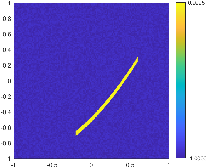
(b) $a^{(2)}_{12}$

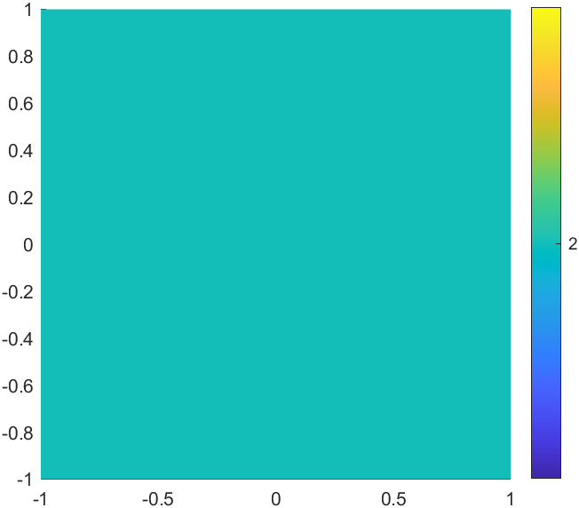
(c) $a^{(2)}_{22}$

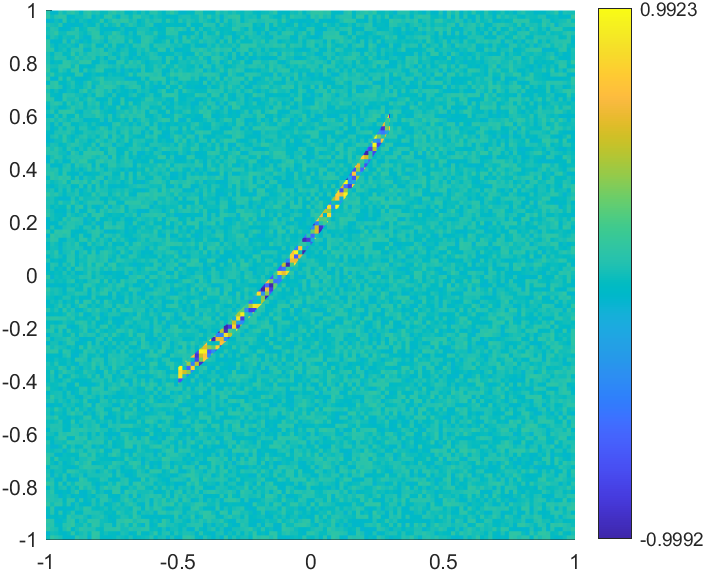
(d) $b^{(2)}_{1}$

(e) $b^{(2)}_{2}$

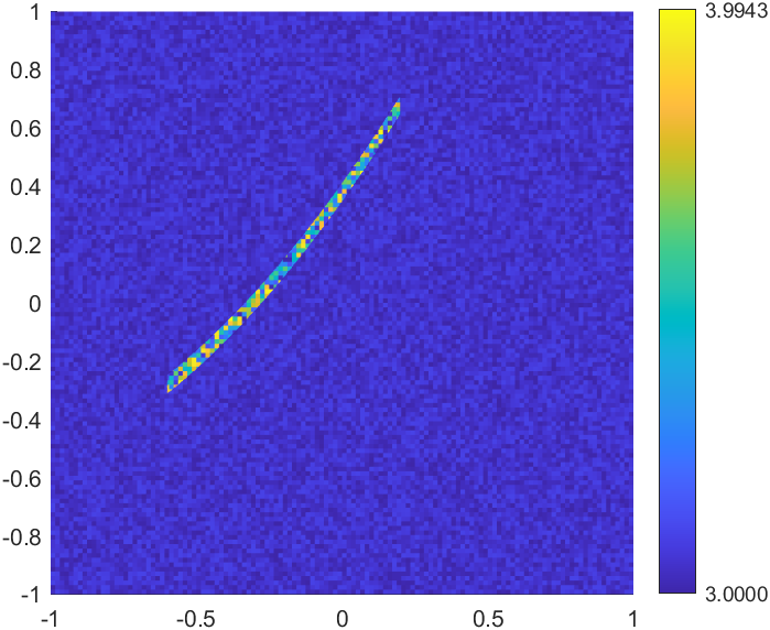
(f) $c^{(2)}$

Figure 3. Illustration of the coefficients chosen in Section 4.4.

Figure 4. Relative errors for the crack problem with vanishing lower-order terms ($A=A^{(2)}$, $b=0$, $c=0$, $f=f^{(2)}$).

Figure 5. Relative errors for the crack problem with non-vanishing lower-order terms ($A=A^{(2)}$, $b=b^{(2)}$, $c=c^{(2)}$, $f=f^{(2)}$) and $\lambda=2$.

4.5. Combined example

The final example combines various types of heterogeneities and the right-hand side is chosen as $f:=f^{(3)}\in L^{2}(\Omega)\backslash H^{1}(\Omega)$. A plot of the chosen coefficients $A:=A^{(3)}$, $b:=b^{(3)}$, and $c:=c^{(3)}$ is given in Figure 6. Note that the Cordes condition (2.4) is satisfied with $\lambda=1$ since

$$\frac{\lvert A^{(3)}\rvert^{2}+\frac{1}{2}\lvert b^{(3)}\rvert^{2}+\left(c^{(3)}\right)^{2}}{\left(\mathrm{tr}(A^{(3)})+c^{(3)}\right)^{2}}\leq\frac{27+\frac{1}{2}+9}{(6+\frac{14}{5})^{2}}=\frac{1}{2+\frac{222}{1825}}\quad\text{a.e. in }\Omega.$$

The corresponding errors are depicted in LABEL:fig:conv_combi_lo.

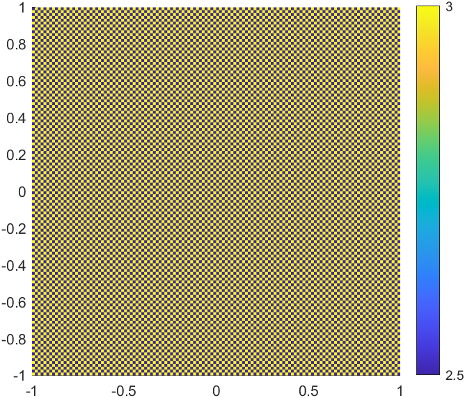
(a) $a^{(3)}_{11}$

(b) $a^{(3)}_{12}$

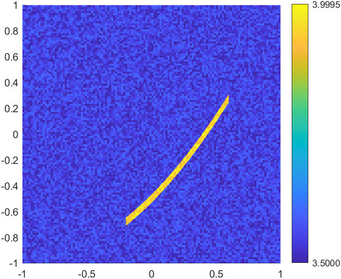
(c) $a^{(3)}_{22}$

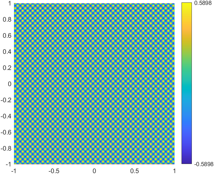
(d) $b^{(3)}_{1}$

(e) $b^{(3)}_{2}$

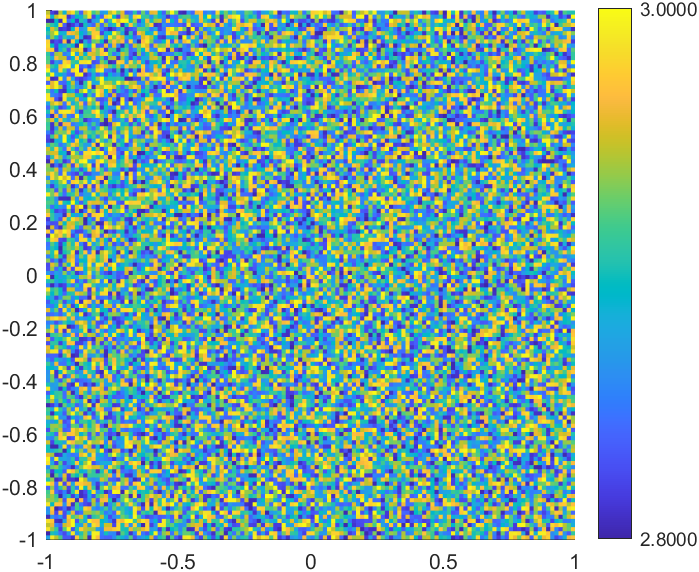
(f) $c^{(3)}$

Figure 6. Illustration of the coefficients chosen in Section 4.5.