beagle-agn I: Simultaneous constraints on the properties of gas in star-forming and AGN narrow-line regions in galaxies

Abstract

We present the addition of nebular emission from the narrow-line regions (NLR) surrounding active galactic nuclei (AGN) to beagle (BayEsian Analysis of GaLaxy sEds). Using a set of idealised spectra, we fit to a set of observables (emission-line ratios and fluxes) and test the retrieval of different physical parameters. We find that fitting to standard diagnostic-line ratios from Baldwin et al. (1981) plus [O ii]$\lambda 3726,\lambda 3729$/[O iii]$\lambda 5007$, H$\beta$/H$\alpha$, [O i]$\lambda 6300$/[O ii]$\lambda 3726,\lambda 3729$ and H$\alpha$ flux, degeneracies remain between dust-to-metal mass ratio ($\xi_{\textnormal{d}}^{\textsc{nlr}}$) and ionisation parameter ($U_{\textnormal{s}}^{\textsc{nlr}}$) in the NLR gas, and between slope of the ionizing radiation ($\alpha_{\textsc{pl}}$, characterising the emission from the accretion disc around the central black hole) and total accretion-disc luminosity ($L_{\textnormal{acc}}$). Since these degeneracies bias the retrieval of other parameters even at maximal signal-to-noise ratio (S/N), without additional observables, we suggest fixing $\alpha_{\textsc{pl}}$ and dust-to-metal mass ratios in both NLR and H ii regions. We explore the S/N in H$\beta$ required for un-biased estimates of physical parameters, finding that S/N$(\hbox{H$\beta$})\sim 10$ is sufficient to identify a NLR contribution, but that higher S/N is required for un-biased parameter retrieval ($\sim 20$ for NLR-dominated systems, $\sim 30$ for objects with approximately-equal H$\beta$ contributions from NLR and H ii regions). We also compare the predictions of our models for different line ratios to previously-published models and data. By adding [He ii]$\lambda 4686$-line measurements to a set of published line fluxes for a sample of 463 AGN NLR, we show that our models with $-4<\hbox{$\log U_{\textsc{s}}^{\textsc{nlr}}$}<-1.5$ can account for the full range of observed AGN properties in the local Universe.

1 Introduction

In searching for obscured (termed type-2) Active Galactic Nuclei (AGNs), astronomers often exploit ‘BPT’ diagrams, which are named after the founding paper by Baldwin et al. (1981). The scheme proposed in Baldwin et al. (1981), which employs ratios between strong emission line fluxes, was later updated by Veilleux & Osterbrock (1987), who settled on three diagnostic diagrams: [O iii]$\lambda 5007$/H$\beta$ versus [S ii]$\lambda 6717,\lambda 6731$/H$\alpha$, [O iii]$\lambda 5007$/H$\beta$ versus [N ii]$\lambda 6584$/H$\alpha$ and [O iii]$\lambda 5007$/H$\beta$ versus [O i]$\lambda 6300$/H$\alpha$. These diagrams provide clear separation of the different ionizing sources powering the line emission. However, at low metallicities, the regions within the diagnostic diagrams occupied by star-formation and AGN-driven line emission increasingly overlap, muddying the classification (Groves et al., 2006; Feltre et al., 2016; Hirschmann et al., 2019). Therefore, at low masses, or higher redshifts, the standard BPT diagrams will be less helpful to distinguish AGN from star-forming activity. It is therefore important to develop new tools to probe the impact of AGNs on galaxy evolution with the new era of large spectroscopic surveys at high redshifts (e.g. with the James Webb Space Telescope).

Beyond simple classification of galaxy-wide star-formation and AGN-driven line emission, there has been significant progress in deriving physical properties of the star-forming regions themselves (e.g. Kewley et al., 2019; Maiolino & Mannucci, 2019, and references therein). However, progress on the side of AGN gas properties is more limited. The first emission-line calibrations to derive oxygen abundances of type-2 AGNs were supplied by Storchi-Bergmann et al. (1998). The subsequent efforts have proceeded along three avenues: further research of observables to derive physical properties (e.g. from rest-frame UV lines, Dors et al. 2014; or the rest-frame optical, Castro et al. 2017); comparison of emission-line ratios with photoionization models, often searching for a minimum $\chi^{2}$ solution (e.g. for rest-frame UV lines, Nagao et al., 2006b; Matsuoka et al., 2009; Matsuoka et al., 2018); and full Bayesian parameter estimation (Pérez-Montero et al., 2019; Thomas et al., 2018b; Mignoli et al., 2019).

Dors et al. (2020a) used a large sample of type-2 AGNs selected from the Sloan Digital Sky Survey (SDSS, York et al., 2000) to provide the first comparison of methods for deriving oxygen abundances of type-2 AGNs. These methods include the calibrations of Storchi-Bergmann et al. (1998), Castro et al. (2017) and the Bayesian-style method employed by the Hii-Chi-mistry code (Pérez-Montero et al., 2019). They find fairly poor agreement between the different methods as well as no significant trend between a galaxy’s stellar mass and the metallicity of the narrow-line region (NLR) surrounding the AGN.

Dors et al. (2020a) also test a ‘direct’ method, that estimates the electron temperature ($T_{\textnormal{e}}$) within the high-ionization zone using the $R_{\mathrm{O}3}=[\mathrm{O}\textsc{iii}]\lambda 4959\AA,\lambda 5007\AA/\lambda 4363\AA$ ratio. They find that their implemented ‘direct’ method significantly under-estimates the derived metallicities compared to the other methods. In Dors et al. (2015), they inferred that the ‘direct’ metallicities were significantly lower than extrapolated radial metallicity gradients derived from gas-phase abundances. Dors et al. (2020b) subsequently identify the cause of the discrepancy between various calibrations and the ‘direct’ method. They update the ‘direct’ method and demonstrate that the previous discrepancies with other calibrations are much reduced. Further to this, Dors (2021) provide the first strong-line calibration against ‘direct’ metallicity estimates for AGNs.

Despite large discrepancies in different oxygen abundance estimates, there have been efforts to characterise the type-2 AGN population by studying line emission. The first studies investigating the statistics of gas metallicity in the narrow-line region of AGNs mostly indicated a lack of evolution with redshift (Matsuoka et al., 2009; Dors et al., 2014), although they did reveal a luminosity-metallicity relation, where less luminous AGNs (characterised by the [He ii]$\lambda 1640$ luminosity in both these studies) display lower metallicities than their bright counterparts. In a later study, Mignoli et al. (2019) investigated the properties of the NLR gas of a sample of Type-2 AGNs selected in a homogeneous way and found significant evolution with redshift. This study employed a wider selection of lines, as well as updated photoionization models, which better reproduce the [N v]$\lambda 1240$ line without resorting to the very high metallicities evoked in previous studies of quasars (e.g., Hamann & Ferland, 1993; Dietrich et al., 2003; Nagao et al., 2006a) and narrow-line Seyfert-I galaxies (Shemmer & Netzer, 2002). Recently, do Nascimento et al. (2022) used strong-line calibrations to study the NLR in type-2 AGNs within the MaNGA survey (Mapping Nearby Galaxies at Apache Point Observatory; Bundy et al., 2015), finding that the central NLR region typically has lower metallicity than the surrounding HII regions. They posit that this may be due to accretion of metal-poor gas at the centre of these galaxies, which is feeding the central black hole.

One limitation of all the methods mentioned thus far is the lack of any accounting for H ii region contribution to the line emission. Thomas et al. (2018b) explicitly investigate the degree of H ii and NLR mixing in the line emission in a sample of SDSS galaxies using their Bayesian code, NebularBayes. They demonstrate that even in regions of the BPT diagram where AGNs are determined to be cleanly selected, the Balmer lines can have a significant contribution from H ii regions ionized by young stars (see also Agostino et al., 2021). Further to this, Thomas et al. (2019) measure the mass-metallicity relation of type-2 AGNs finding a moderate increase in oxygen abundance with increasing stellar mass.

With this paper, we present the incorporation of the Feltre et al. (2016) NLR models into beagle (BayEsian Analysis of GaLaxy sEds), a tool to model and interpret galaxy spectral energy distributions (Chevallard & Charlot, 2016) (Section 2). This addition allows the mixing of line emission from young stellar birth clouds (Section 2.1) with that from the NLR of type-2 AGNs (Section 2.2). beagle also self-consistently includes stellar emission and attenuation by interstellar dust (Section 2.3), which are not explicitly modelled in NebularBayes.

In Section 3, we take a pedagogical approach to defining what parameters of our model can be constrained by fitting a given set of observables (Section 3.2) in idealised spectra (Section 3.1). Using such spectra, we quantify the S/N required to constrain H ii-region and NLR-gas parameters for different NLR contributions to the total H$\beta$ flux of a galaxy (Sections 3.3 and 3.4). With this work, we focus on rest-frame optical observables, though beagle can also be used to study emission lines from the rest-frame UV. Finally, we compare the results of our model with those obtained using previously published methods in Section 4 and expand on the comparison work of Dors et al. (2020a) by explaining how different methods will derive different oxygen abundances (Section 4.1). In particular, in Section 4.2 we compare several emission-line ratios and several free parameters in the models and in a set of type-2 AGN observations. In order to explain different trends for the ionization parameter, in Section 4.3 we present new measurements of the [He ii]$\lambda 4686$ fluxes in a few hundred type-2 AGNs from DR7 SDSS and we compare the measured data to the fluxes predicted by the F16 models. We also show the predictions of the fluxes for sulfur and nitrogen lines in Section 4.4, and end this discussion (Section 4.5) by comparing the Dors (2021) empirical $T_{\textnormal{e}}$-based $12+\log(\textnormal{O}/\textnormal{H})$ calibration to the different model grids. The paper ends in Section 5 with a summary of the main findings of this work. This is the first in a series of three papers, to be followed by a paper on fitting of a sample of type-2 AGNs with beagle, and a study of the extent to which line emission from shocks and post-AGB stars may affect our inferences.

2 Modelling the emission from stars, H ii regions and AGN NLRs in beagle

beagle (Chevallard & Charlot, 2016, hereafter CC16) is a Bayesian SED-fitting code, which allows efficient exploration of a wide grid of physical parameters affecting the light emitted by a galaxy. The code employs MultiNest (a Bayesian analysis tool based on the Nested Sampling algorithm of Skilling et al. 2006; see Feroz et al., 2009) to sample from the posterior probability distributions of physical parameters. We refer the reader to CC16 for more details.

A main feature of beagle is the incorporation of physically consistent stellar continuum and nebular emission models, which trace the production of starlight and its transmission through the interstellar medium self-consistently. This paper is concerned with the extension of beagle to allow for the interpretation of mixed emission-line signatures of AGNs and stars. In Section 2.1 below, we briefly review the modelling of the emission from stars and H ii regions in beagle, while in Section 2.2, we describe our incorporation of the emission from AGN narrow-line regions.

2.1 Emission from stars and H ii regions

beagle employs the latest version of the Bruzual & Charlot (2003) stellar population synthesis models (as described in Vidal-García et al., 2017) to compute the emission from stars.

The line and continuum emission of H ii regions ionized by stars younger than 10 Myr is computed following the prescription of Gutkin et al. (2016, see also ) for a grid of gas parameters: the metallicity of the H ii-region gas, $\hbox{$\textnormal{Z}$}_{\textnormal{gas}}^{\textsc{hii}}$ (noted $\hbox{$\textnormal{Z}$}_{\textsc{ism}}$ in Gutkin et al. 2016); the ionization parameter, $\log U_{\textsc{s}}$; and the dust-to-metal mass ratio within the H ii regions, $\xi_{\textnormal{d}}$. Nitrogen abundances are scaled to oxygen abundances according to the formula:

$${\rm N/H}\simeq 0.41\,{\rm O/H}\left[10^{-1.6}+10^{(2.33+\log\rm O/H)}\right]\,,$$ (1)

which well matches the relation between N/O and $12+\log(\textnormal{O}/\textnormal{H})$ in observed H ii regions (see equation 11 and figure 1 of Gutkin et al., 2016).

For simplicity, we fix here the carbon-to-oxygen ratio of the H ii regions to solar, $\hbox{(C/O)${}_{\odot}$}=0.44$, and the hydrogen density to $\hbox{$n_{\textsc{h}}$}=100\,$cm^-3. In the stellar population models, we fix the upper limit of the stellar initial mass function (IMF) to 100 $\rm\thinspace M_{\odot}$. An important feature of this grid is the coupling of stellar light to its transmission through the interstellar medium (ISM), via not only the nebular emission, but also the attenuation by dust in the H ii regions themselves (see Section 2.3).

2.2 Emission from AGN narrow-line regions

We appeal to the Feltre et al. (2016, hereafter F16) models of AGN-NLR emission to introduce simultaneous fitting of the physical properties of NLR and H ii regions with beagle. The F16 NLR models were produced with cloudy c13.03 (Ferland et al., 2013, the same version as used by Gutkin et al. 2016 to produce the H ii-region models). Three important aspects must be considered to incorporate the treatment of NLR emission into beagle: the shape of the AGN ionizing continuum; the properties of the NLR gas itself; and the integration of the F16 model grid with the H ii-region model grid within beagle. In the next paragraphs, we summarise the salient features of our approach to achieve these goals.

In the F16 model, the radiation illuminating the NLR gas is the thermal emission from the accretion disc surrounding the central black hole. For simplicity, this emission is described by a broken power law, as shown in Fig. 1 (see also equation 5 of F16). The strengths of emission lines emerging from the NLR, as well as the ratios between them, are primarily sensitive to the slope, $\alpha_{\textsc{pl}}$, of the power law at high frequencies (short wavelengths). F16 allow this parameter to vary in the range $-1.2<\hbox{$\alpha_{\textsc{pl}}$}<-2.0$, which are generally used as “standard” values for the power-law slope (e.g. Groves et al., 2004).

Figure 1: The incident radiation used to compute different NLR emission models. The models of F16 are used in this work, and allow a range of slope ($\alpha_{\textsc{pl}}$) of the ionizing portion of the spectrum. The F16 models use a simplified parametric form which describes the thermal emission from the accretion disc surrounding the central black hole. We use a model grid that includes a range of spectral indices, $\alpha_{\textsc{pl}}$, in the rest-frame UV to soft X-ray [$\log(\nu/\textnormal{Hz})\gtrsim 15$], as indicated. The shape is described in Schartmann et al. (2005) and Feltre et al. (2012). We also plot the incident radiation used in a number of different works for comparison, as specified in the legend. We compare the emission line ratios of these different models to observations in Section 4.

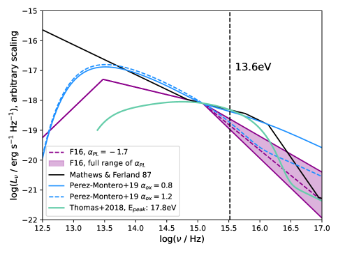
This simplified description of the purely thermal emission from the accretion disc does not attempt to model the hard X-ray component thought to arise from the Comptonization of photons scattered in the hot corona surrounding the disc (Haardt & Maraschi, 1991). A soft X-ray component is also often observed in AGNs, the exact nature of which is still debated (e.g., disc reflection, Crummy et al. 2006; or optically-thick Comptonized disc emission, which can explain the soft X-ray excess in narrow-line Seyfert-Is, Done et al. 2012). In practice, the flexibility in $\alpha_{\textsc{pl}}$ allows the exploration of different contributions of soft X-rays to the incident ionizing radiation.

Once the spectrum of the accretion-disc radiation reaching the NLR is defined, cloudy can be used to model the transfer of this radiation through the NLR gas. The F16 NLR grid employs the option of ‘open geometry’, suitable for gas with low covering fraction. The models are computed for a typical accretion luminosity (i.e., the integral of the broken power law in Fig. 1) of $\hbox{$L_{\textnormal{acc}}$}=10^{45}\,\hbox{$\textrm{erg}\,\textrm{s}^{-1}\,\textrm{cm}^{-2}$}$ (denoted $L_{\textnormal{AGN}}$ in F16). The version of the F16 model incorporated into beagle includes further updates by Mignoli et al. (2019) which better account for the observed [N v]$\lambda 1240$/[He ii]$\lambda 1640$ emission-line ratios in a sample of high-redshift type-2 AGNs. Specifically, the inner radius of the gas is set to $r_{\textnormal{in}}\approx 90\,\textrm{pc}$, and the internal micro-turbulence velocity to $v_{\textnormal{micr}}=100\,\textrm{km}\,\textrm{s}^{-1}$.

To incorporate nebular emission from AGN NLR into beagle, we use a grid of F16 models covering full ranges in $\alpha_{\textsc{pl}}$ and other NLR-gas parameters: the metallicity, noted $\hbox{$\textnormal{Z}$}_{\textnormal{gas}}^{\textsc{nlr}}$; the ionization parameter, $\log U_{\textsc{s}}^{\textsc{nlr}}$; and the dust-to-metal mass ratio, $\xi_{\textnormal{d}}^{\textsc{nlr}}$. In this work, we fix the hydrogen density in the NLR to $\hbox{$n_{\textsc{h}}^{\textsc{nlr}}$}=1000$ cm^-3, as typically measured from optical line doublets (Osterbrock & Ferland, 2006). Furthermore, as for the H ii regions (Section 2.1), we fix the C/O abundance ratio in the NLR gas to solar and use equation (1) to describe the dependence of N/H on O/H. Table 1 lists the full set of physical parameters pertaining to the H ii and NLR regions in our models.

Table 1: List of physical parameters used in this work to simulate and fit to (active and inactive) galaxy spectra.

Parameter	Description
$\hbox{$\textnormal{M}_{\textnormal{tot}}$}/\hbox{$\rm\thinspace M_{\odot}$}$	Integrated SFH.
M/$\rm\thinspace M_{\odot}$	Stellar mass, including stellar remnants.
$\hbox{${\psi}$}/\hbox{$\rm\thinspace M_{\odot}$}\mathrm{yr}^{-1}$	Current star formation rate.
$\hbox{$\hbox{$\textnormal{Z}$}_{\textnormal{gas}}^{\textsc{hii}}$}/\hbox{$\hbox{$\textnormal{Z}$}_{\odot}$}$, $\hbox{$\hbox{$\textnormal{Z}$}_{\textnormal{gas}}^{\textsc{nlr}}$}/\hbox{$\hbox{$\textnormal{Z}$}_{\odot}$}$	Metallicity of gas in H ii regions and the NLR, respectively.
$\hat{\tau}_{\textsc{v}}$	Total $V$-band attenuation optical depth in the ISM.
$\mu$	Fraction of $\hat{\tau}_{\textsc{v}}$ arising from dust in the diffuse ISM, fixed to 0.4.
$\log U_{\textsc{s}}$, $\log U_{\textsc{s}}^{\textsc{nlr}}$	Effective gas ionization parameter in H ii regions and the NLR, respectively.
$\xi_{\textnormal{d}}$, $\xi_{\textnormal{d}}^{\textsc{nlr}}$	Dust-to-metal mass ratio in H ii regions and the NLR, respectively.
$\hbox{$n_{\textsc{h}}$}/\mathrm{cm}^{-3}$, $\hbox{$n_{\textsc{h}}^{\textsc{nlr}}$}/\mathrm{cm}^{-3}$	Hydrogen gas density in H ii regions (fixed to 100) and the NLR (fixed to 1000), respectively.
(C/O)/(C/O)⊙	Carbon-to-oxygen abundance ratio in units of (C/O)${}_{\odot}=0.44$, fixed to unity.
$m_{\mathrm{up}}/\hbox{$\rm\thinspace M_{\odot}$}$	Upper mass cutoff of the IMF, fixed to 100.
$t$/Gyr	Age of the oldest stars.
$\alpha_{\textsc{pl}}$	Slope of the ionizing radiation from thermal emission of the accretion disc around the central black hole.
$L_{\textnormal{acc}}$	Integrated thermal emission from the accretion disc.

In combining the H ii-region and NLR model grids in beagle, we allow for the normalisation of the NLR models to change. In practice, we achieve this by changing the parameter $L_{\textnormal{acc}}$, which controls the absolute luminosities of NLR emission lines (Table 1). We note that this is compatible with the adoption of a fixed $\hbox{$L_{\textnormal{acc}}$}=10^{45}\,\hbox{$\textrm{erg}\,\textrm{s}^{-1}\,\textrm{cm}^{-2}$}$ in the photoionization calculations of F16. Indeed, we find that, at fixed other parameters, the emission-line luminosities computed with cloudy for values of $L_{\textnormal{acc}}$ in the range from $10^{42}$ to $10^{48}\,\hbox{$\textrm{erg}\,\textrm{s}^{-1}\,\textrm{cm}^{-2}$}$ differ by only 0.1 to 6 per cent (depending on the considered line) from those obtained by simply scaling the luminosities of a model with $\hbox{$L_{\textnormal{acc}}$}=10^{45}\,\hbox{$\textrm{erg}\,\textrm{s}^{-1}\,\textrm{cm}^{-2}$}$. This is because we assume a fixed scaling relation between the inner radius of the ionized gas ($r_{\rm in}$) and $L_{\textnormal{acc}}$, given by $L_{\textnormal{acc}}$$/(4\pi r_{\rm in}^{2})\simeq 10^{2}\,\hbox{$\textrm{erg}\,\textrm{s}^{-1}\,\textrm{cm}^{-2}$}$ (Feltre et al., 2016). We must also account for the inhomogeneous distribution of the narrow-line emitting gas around the central AGN. This can be achieved by multiplying $L_{\textnormal{acc}}$ by a gas covering fraction, whose recovery from observables will however be degenerate with $L_{\textnormal{acc}}$. To avoid introducing this extra degeneracy when fitting to data with beagle, we fix the covering fraction of NLR gas to 10 per cent, which is within the range of values (2-20$\%$) obtained for the covering fraction of the NLR gas of the Palomar-Green quasar sample (Baskin & Laor, 2005).

Since we are modelling type-2 AGNs, we are focused on modelling the narrow line-emitting region. Continuum emission from the accretion disc itself is assumed to be completely obscured by the dust surrounding the AGN centre, often referred to as the AGN torus. Any non-ionizing continuum light (of the form in Fig. 1) that is reflected from the NLR is included in the models, however, its contribution to most SEDs is negligible relative to the stellar continuum in practice. For simplicity, we assume that the radiation by the accretion disc and surrounding NLR gas are spherically symmetric. This is a reasonable assumption when teamed with the covering fraction, but does not take account of scattering or absorption of the accretion disc radiation by the dust in the torus, nor of the anisotropic nature of the emission from the accretion disc itself.

2.3 Attenuation by dust

In this work, we adopt the Charlot & Fall (2000, hereafter CF00) two-component dust model. This model accounts for the enhanced dust content in stellar birth clouds compared to the diffuse ISM. The dust within birth clouds is split between the inner H ii and outer H i regions, with the dust in H ii regions being self-consistently accounted for in the nebular emission grid of Gutkin et al. (2016). As of beagle v0.27.1, this dust component is accounted for self-consistently within the implementation of the CF00 model, as described in Curtis-Lake et al. (2021).

When combining NLR emission with the emission from stars we account for the dust both within the NLR and the diffuse ISM. As for the H ii region models, dust is included in the F16 cloudy models of the NLR. Hence, within beagle, in the framework of the CF00 dust model, light emitted from the NLR is subject only to further attenuation by dust in the diffuse ISM.

3 Retrieval of parameters from idealised models

3.1 Idealised models of active galaxies

Table 2: Properties of the idealised models of active galaxies at $z=0$ and $z=2$ used to test parameter retrieval with beagle.

Parameter	$z=0$	$z=2$
$\log(\hbox{$\textnormal{M}$}/\hbox{$\rm\thinspace M_{\odot}$})$	10.5	10.5
$\hbox{${\psi}$}/\hbox{$\rm\thinspace M_{\odot}$}\mathrm{yr}^{-1}$	0.4	1.3
$\hbox{$\textnormal{Z}$}_{\textnormal{gas}}^{\textsc{hii}}$	0.014	0.007
$\log U_{\textsc{s}}$	$-3.6$	$-3.0$
$\hbox{$n_{\textsc{h}}$}/\textnormal{cm}^{-3}$	100	100
$\xi_{\textnormal{d}}$	0.3	0.3
$t$/Gyr	10	1
$\hbox{$\textnormal{Z}$}_{\textnormal{gas}}^{\textsc{nlr}}$	0.030	0.012
$\log U_{\textsc{s}}^{\textsc{nlr}}$	$-3.5$	$-2.75$
$\hbox{$n_{\textsc{h}}^{\textsc{nlr}}$}/\textnormal{cm}^{-3}$	1000	1000
$\xi_{\textnormal{d}}^{\textsc{nlr}}$	0.3	0.3
$\hat{\tau}_{\textsc{v}}$	0.3	0.3
$\mu$	0.4	0.4
$\alpha_{\textsc{pl}}$	$-1.7$	$-1.7$

Figure 2: Histograms of the physical parameter space covered by galaxies in IllustrisTNG-100 at z=0 (top row) and z=2 (bottom row). Dashed vertical lines indicate the mean value of each quantity, while the solid black lines indicate the values used.

Figure 3: The [N ii]$\lambda 6584$, [S ii]$\lambda 6717,\lambda 6731$ and [O i]$\lambda 6300$ BPT diagrams showing the coverage of galaxies within SDSS as grey filled contours. Violet symbols show pure NLR models chosen to represent typical AGNs at $z=0$ (circles) and $z=2$ (stars), while orange symbols show the models chosen to represent typical star-forming galaxies at the same redshifts. The parameters chosen to represent these galaxies are motivated by the IllustrisTNG-100 simulation (see text for details). The points spanning between the two extremes show different contributions of NLR model to the corresponding star-forming model, parametrized by the fractional contribution of NLR to the H$\beta$ flux (as described in the legend).

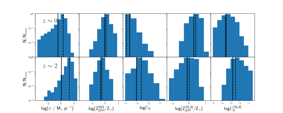
To investigate how well we can identify type-2 AGNs and constrain their NLR properties at different redshifts, we choose to model two ‘typical’ star-forming galaxies at $z=0$ and $z=2$, to which we add various levels of AGN contribution. We select the input parameters of these models by appealing to the IllustrisTNG-100 cosmological, magneto-hydrodynamic simulation of galaxy formation (Springel et al., 2018; Pillepich et al., 2018; Naiman et al., 2018; Nelson et al., 2018; Marinacci et al., 2018). See Hirschmann et al. in prep. for the details of how these parameters have been retrieved (see also Hirschmann et al., 2017; Hirschmann et al., 2019). Fig. 2 shows histograms of selected physical properties of galaxies with stellar masses at least $3\times 10^{9}$$\rm\thinspace M_{\odot}$ extracted from this simulation.

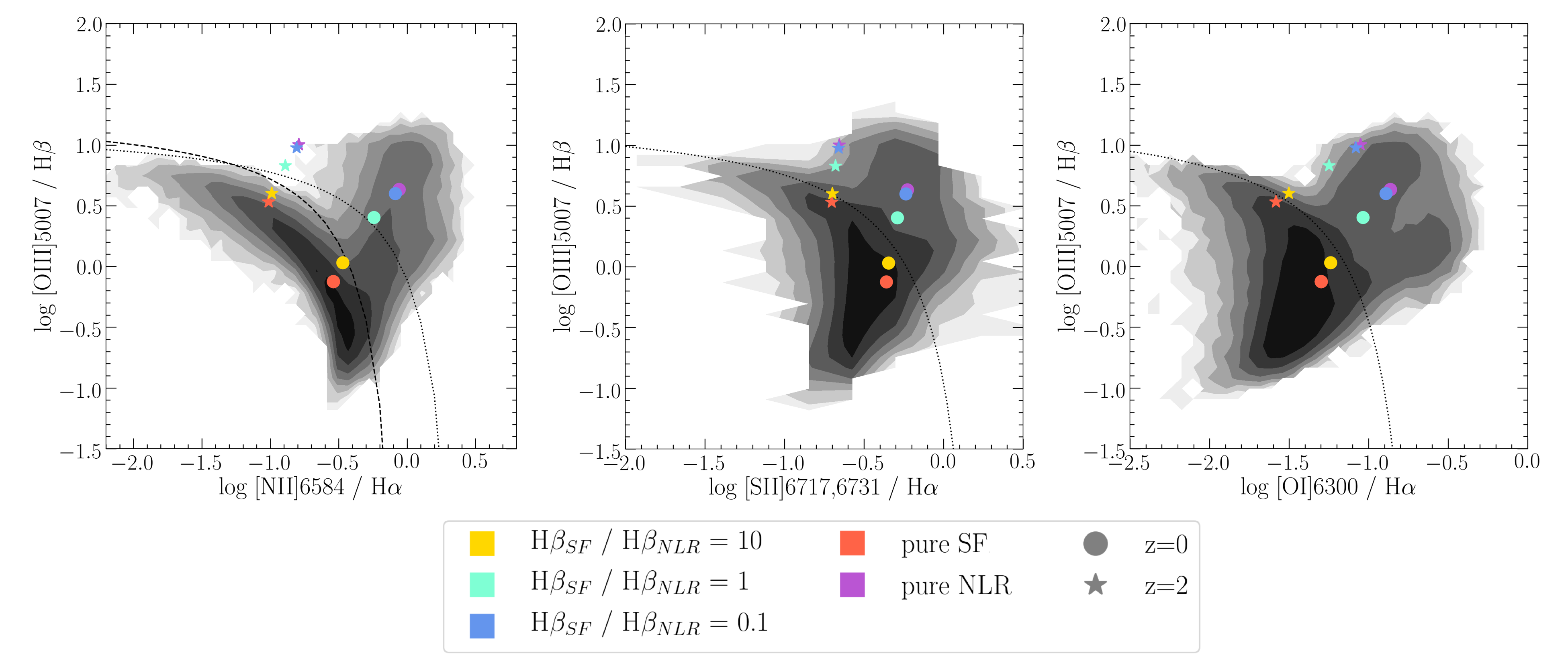
We fix the stellar masses of both $z=0$ and $z=2$ galaxies to $\log(\hbox{$\textnormal{M}$}/\hbox{$\rm\thinspace M_{\odot}$})=10.5$, corresponding to just below the turnover of the stellar mass function of star-forming galaxies measured over this redshift range (e.g. Tomczak et al., 2014). Setting the ages of the oldest stars to 10 Gyr at $z=0$ and 1 Gyr at $z=2$ ensures that the objects are younger than the Universe. The star formation history is parametrized as constant, with an ongoing uncoupled 10-Myr burst of star formation. We take the current star formation rates of the $z=0$ and 2 galaxies to correspond to the mean values from the Illustris simulation at these redshifts, i.e., $\hbox{${\psi}$}\approx 0.4$ and $1.3\hbox{$\rm\thinspace M_{\odot}$}$ yr^-1, respectively. The distributions of $\hbox{$\textnormal{Z}$}_{\textnormal{gas}}^{\textsc{hii}}$ and $\log U_{\textsc{s}}$ for star-forming galaxies at $z\sim 0$ and 2 in the Illustris simulation are fairly broad and allow for some freedom in choosing typical values. We adopt values of $\hbox{$\textnormal{Z}$}_{\textnormal{gas}}^{\textsc{hii}}$ and $\log U_{\textsc{s}}$ such that the purely star-forming models lie on the sequence of SDSS star-forming galaxies in the classical [N ii]$\lambda 6584$/H$\alpha$ BPT diagram (see Fig. 3). For the AGN component, we adopt the mean $\hbox{$\textnormal{Z}$}_{\textnormal{gas}}^{\textsc{nlr}}$ from Illustris at each redshift and tweak $\log U_{\textsc{s}}^{\textsc{nlr}}$ to ensure that the models sample the AGN portion of the [O i]$\lambda 6300$/H$\alpha$ BPT (rather than the LINER/shock region at lower [O ii]$\lambda 3726,\lambda 3729$/H$\beta$ and higher [O i]$\lambda 6300$/H$\alpha$).

Among the other parameters remaining to be specified, the C/O abundance ratio is fixed to solar, the hydrogen densities in the H ii-region and NLR gas to $\log(\hbox{$n_{\textsc{h}}$}/\textrm{cm}^{-3})=2$ and 3, respectively, and the upper mass cutoff of the IMF to 100$\rm\thinspace M_{\odot}$ (see Sections 2.1 and 2.2). We further fix the dust-to-metal mass ratio to $\hbox{$\xi_{\textnormal{d}}$}=\hbox{$\xi_{\textnormal{d}}^{\textsc{nlr}}$}=0.3$, the V-band attenuation optical depth and its fraction arising from the dust in the ambient ISM to $\hbox{$\hat{\tau}_{\textsc{v}}$}=0.3$ and $\mu=0.4$ respectively. Finally, we set the power-law slope of the accretion-disc emission model to $\hbox{$\alpha_{\textsc{pl}}$}=-1.7$, in the middle of the range probed by the AGN-NLR model (Section 2.2). Table 2 summarises the parameters of these idealised models.

When combining the H ii-region and NLR models, we consider three types of galaxies at each redshift: one for which line emission is dominated by star formation, one for which it is dominated by the NLR, and one with equal contribution. We set the ratio of H$\beta$ luminosities from H ii regions and the NLR be $\hbox{H$\beta$}^{\textnormal{HII}}/\hbox{H$\beta$}^{\textnormal{NLR}}=0.1$, 1 and 10. This ensures that our models bridge the space between the regions dominated by star-forming galaxies and AGNs in the BPT. We ensure the highest value of $L_{\textnormal{acc}}$ (obtained for $\hbox{H$\beta$}^{\textnormal{HII}}/\hbox{H$\beta$}^{\textnormal{NLR}}=0.1$) is lower than the Eddington luminosity,

$$L_{\mathrm{Edd}}=\dfrac{4\pi Gcm_{\mathrm{p}}}{\sigma_{\mathrm{e}}}\hbox{$M_{\textsc{bh}}$}\approx 1.26\times 10^{38}(\hbox{$M_{\textsc{bh}}$}/\hbox{$\rm\thinspace M_{\odot}$})\,\mathrm{erg\,s}^{-1}\,,$$ (2)

where $M_{\textsc{bh}}$ is the black-hole mass, $c$ the speed of light, $m_{\mathrm{p}}$ the proton mass and $\sigma_{\mathrm{e}}$ the Thomson-scattering cross-section for electrons. In the local Universe, the mass of the central black hole in active galaxies tends to scale with total stellar mass as $\hbox{$M_{\textsc{bh}}$}\sim 0.025\hbox{$M_{\star}$}$ (e.g. Reines & Volonteri, 2015). Hence, the condition $\hbox{$L_{\textnormal{acc}}$}<L_{\textnormal{Edd}}$ requires the galaxy stellar mass to be at least $\sim 40$ times the corresponding black-hole mass in equation (2), which is the case in our models at both redshifts.

Finally, we also add flat noise to the synthetic spectra, which we parametrize in terms of the observed H$\beta$ signal-to-noise ratio, S/N(H$\beta$). The standard deviation of the noise per pixel, $\sigma_{\mathrm{N}}$, is linked to S/N(H$\beta$) through the formula (e.g. Hagen et al., 2007)

$$\sigma_{\mathrm{N}}=\sqrt{\dfrac{2w_{\beta}\delta\sqrt{\pi}A_{\beta}^{2}}{3\mathrm{[S/N(\hbox{H$\beta$})]}^{2}}}\,,$$ (3)

where $w_{\beta}$ is the H$\beta$ line width, $\delta$ the pixel width and $A_{\beta}$ the amplitude of the line. Throughout this work, we investigate the effect of S/N(H$\beta$) on derived properties.

At low $\textrm{S/N(H}\beta)$, the perturbed line fluxes for weak lines can fluctuate significantly. To mitigate this effect, we produce 10 spectra for each $\textrm{S/N(H}\beta)$ threshold and average the results after having fitted to the spectra with beagle.

3.2 Fitting with beagle

Our aims when fitting with beagle are two-fold. First we hope to distinguish objects with an obscured-AGN component contributing to the emission-line fluxes. Additionally we wish to constrain the gas properties of the NLR and star-forming regions. Our base set of observables are the lines used to make the three emission-line diagnostic diagrams identified by Baldwin et al. (1981) for distinguishing the dominant ionizing source, namely [O iii]$\lambda 5007$, [O i]$\lambda 6300$, H$\alpha$, H$\beta$, [N ii]$\lambda 6584$ and [S ii]$\lambda 6717,\lambda 6731$. We add the [O ii]$\lambda 3726,\lambda 3729$ emission line doublet to gain constraints on the ionization state of the gas (most directly together with [O iii]$\lambda 5007$ for constraints on $\log U_{\textsc{s}}$ and $\log U_{\textsc{s}}^{\textsc{nlr}}$). We measure these line fluxes and associated uncertainties from the noisy spectra described in section 3.1 using PySpecLines. Specifically, we fit Gaussian profiles to each of the lines, simultaneously fitting multiple lines that are close or overlapping in the spectrum. We employ the mcmc option in PySpecLines for the line fitting to ensure realistic uncertainty estimates.

From a first analysis we found that fitting to individual line fluxes produces biased estimates of AGN parameters, and so we construct the likelihood using line ratios particularly sensitive to the estimated physical parameters. In particular, we use: the BPT line ratios [O i]$\lambda 6300$/H$\alpha$, [N ii]$\lambda 6584$/H$\alpha$, [S ii]$\lambda 6717,\lambda 6731$/H$\alpha$ and [O iii]$\lambda 5007$/H$\beta$; H$\beta$/H$\alpha$ to provide constraints on dust attenuation; [O i]$\lambda 6300$/[O ii]$\lambda 3726,\lambda 3729$ and [O ii]$\lambda 3726,\lambda 3729$/[O iii]$\lambda 5007$ to provide constraints on the ionization parameters. To constrain the absolute normalisation of the line fluxes, we also include the comparison of H$\alpha$ flux in the likelihood calculations. The above line ratios produce improved estimates of various parameters thanks to the higher weighting of lines in the partially ionized zone ([N ii]$\lambda 6584$, [S ii]$\lambda 6717,\lambda 6731$, [O i]$\lambda 6300$) to the likelihood evaluation. When these lines are faint and not fitted as line-ratios but rather individually, the information in the likelihood is dominated by stronger lines which contain less information about the NLR properties (H$\alpha$, H$\beta$, [O ii]$\lambda 3726,\lambda 3729$). We make the simplifying assumption that the line ratios are independent. The method of using line ratios in this way is similar to that adopted by other works, such as Pérez-Montero et al. (2019).

Within the likelihood determination, we assume that the measurement of the ratio is Gaussian-distributed, with $\mu$ the mean and $\sigma$ the standard deviation of the distribution. The ratio between two Gaussian-distributed variables, $Z=X/Y$ [where $X\sim\mathcal{N}(\mu_{x},\sigma^{2}_{x})$ and $Y\sim\mathcal{N}(\mu_{y},\sigma^{2}_{y})$], is strictly described by a Cauchy distribution when the mean of each distribution is zero. However, the distribution of the ratio of two independent normal random variables can be approximated as a Gaussian with variance:

$$\sigma^{2}_{z}=\frac{\mu_{x}^{2}}{\mu_{y}^{2}}\left(\frac{\sigma_{x}^{2}}{\mu_{x}^{2}}+\frac{\sigma_{y}^{2}}{\mu^{2}_{y}}\right)$$ (4)

when $0<\sigma_{x}/\mu_{x}<\lambda\leq 1$ and $0<\sigma_{y}/\mu_{y}\leq\sqrt{\lambda^{2}-\sigma_{x}^{2}/\mu_{x}^{2}}<\lambda$, where $\lambda$ is a constant between zero and one (Díaz-Francés & Rubio, 2013), and $\sigma/\mu$ is equal to the inverse of the S/N on the given parameter. We always choose ratios with the lower S/N line as the numerator, which safely respects the condition on $\sigma_{x}/\mu_{x}$. Re-writing the central part of the second condition using $\sigma_{y}/\mu_{y}=\frac{1}{N}\sigma_{x}/\mu_{x}$ (which is equivalent to saying the signal-to-noise on $y$ is a multiple of $N$ times higher than the signal-to-noise on $x$), we have $\sqrt{(N^{2}+1)}\sigma_{x}/\mu_{x}<N\lambda$, which is trivially true if $N>1$ and $\sigma_{x}/\mu_{x}<\lambda$. Therefore, we are generally within the regime where we can safely model the distribution of the line ratios as a Gaussian. In practice, the lines on the numerator do not always satisfy $\sigma_{x}/\mu_{x}<1$. However, when they have very low S/N (high $\sigma_{x}/\mu_{x}$), their weighting within the likelihood is much lower and so this should not significantly affect the results.

Table 3: Uniform prior limits and fixed values applied to the three different fits for different parameters in beagle.

Parameter	Fit $\alpha_{\textsc{pl}}$	Fit $\xi_{\textnormal{d}}^{\textsc{nlr}}$	Fixed $\alpha_{\textsc{pl}}$and $\xi_{\textnormal{d}}^{\textsc{nlr}}$
$\hbox{$\hbox{$\textnormal{M}$}_{\textnormal{tot}}$}=\log(\hbox{$\textnormal{M}_{\textnormal{tot}}$}/\hbox{$\rm\thinspace M_{\odot}$})$	Uniform $\in[7,13]$	$\in[7,13]$	$\in[7,13]$
$\hbox{${\Psi}$}=\log(\hbox{${\psi}$}/\hbox{$\rm\thinspace M_{\odot}$}\hbox{$\textnormal{yr}$}^{-1})$	Uniform $\in[-4.,4.]$	Uniform $\in[-4.,4.]$	Uniform $\in[-4.,4.]$
$\log(\hbox{$\hbox{$\textnormal{Z}$}_{\textnormal{gas}}^{\textsc{hii}}$}/\hbox{$\hbox{$\textnormal{Z}$}_{\odot}$})$	Uniform $\in[-2.2,0.24]$	Uniform $\in[-2.2,0.24]$	Uniform $\in[-2.2,0.24]$
$\log(\hbox{$t$}/\hbox{$\textnormal{yr}$})$	Uniform $\in[6,11]$	Uniform $\in[6,11]$	Uniform $\in[6,11]$
$\log U_{\textsc{s}}$	Uniform $\in[-4,-1]$	Uniform $\in[-4,-1]$	Uniform $\in[-4,-1]$
$\xi_{\textnormal{d}}$	Fixed to 0.3	Fixed to 0.3	Fixed to 0.3
$\hat{\tau}_{\textsc{v}}$	Uniform $\in[0,2]$	Uniform $\in[0,2]$	Uniform $\in[0,2]$
$\mu$	Uniform $\in[0,1]$	Uniform $\in[0,1]$	Uniform $\in[0,1]$
$\log(\hbox{$L_{\textnormal{acc}}$}\/\hbox{\,${\rm L}_{\odot}$})$	Uniform $\in[40,48]$	Uniform $\in[40,48]$	Uniform $\in[40,48]$
$\xi_{\textnormal{d}}^{\textsc{nlr}}$	Fixed to 0.3	Uniform $\in[0.1,0.5]$	Fixed to 0.3
$\log U_{\textsc{s}}^{\textsc{nlr}}$	Uniform $\in[-4,-1.5]$	Uniform $\in[-4,-1.5]$	Uniform $\in[-4,-1.5]$
$\log(\hbox{$\hbox{$\textnormal{Z}$}_{\textnormal{gas}}^{\textsc{nlr}}$}/\hbox{$\hbox{$\textnormal{Z}$}_{\odot}$})$	Uniform $\in[-2.2,0.24]$	Uniform $\in[-2.2,0.24]$	Uniform $\in[-2.2,0.24]$
$\alpha_{\textsc{pl}}$	Uniform $\in[-2.0,-1.2]$	Fixed to -1.7	Fixed to -1.7

3.3 High-quality spectra with S/N(H$\beta$)=100

3.3.1 AGN versus star-formation dominated spectra

(a) $z=0$

(b) $z=2$

Figure 4: Triangle plots of the parameter retrieval for the $z=0$ (left) and $z=2$ (right) NLR-dominated galaxies with S/N$\sim 100$ in H$\beta$. Only NLR parameters are displayed even though SF parameters are also included in the fits. The triangle plots display the average parameter constraints relative to the input values from fits to 10 realisations of noisy spectrum. The crosses show the average bias for each parameter pair, while the ovals show the $1\sigma$ contour of the bi-variate Gaussian fitted to the joint posteriors (see text for details about how this plot is made). These show an approximate representation of the biases and degeneracies between different parameters. We display the results for different combinations of fixed or fitted $\xi_{\textnormal{d}}^{\textsc{nlr}}$ and $\alpha_{\textsc{pl}}$, as specified in the legend.

(a) $z=0$

(b) $z=2$

Figure 5: As in fig. 4, but showing triangle plots of the parameter retrieval for the $z=0$ (left) and $z=2$ (right) star-formation dominated galaxies. We display only SF parameters, though NLR parameters were also included in the fits. Results when $\xi_{\textnormal{d}}$ is both fixed and fitted are displayed according to the legend.

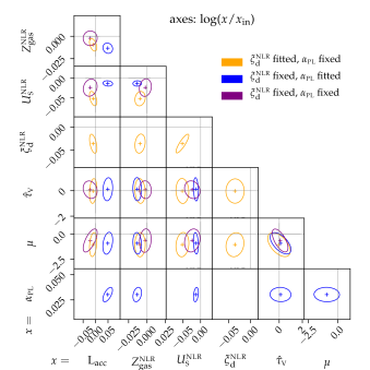
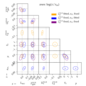
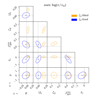
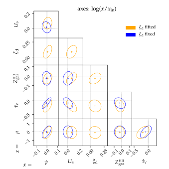
We start by investigating the idealised scenario of high-S/N spectra with full coverage of the lines of interest. From our grid of models, we test the retrieval of physical parameters for the AGN and star-formation dominated cases ($\hbox{H$\beta$}_{\textsc{sf}}/\hbox{H$\beta$}_{\textsc{nlr}}=0.1$ and 0.9, respectively) with high S/N spectra [S/N(H$\beta$)=100]. At this S/N in H$\beta$  we reach $\textrm{S/N}>10$ in all lines used in the analysis. We fit all components (H ii, stellar continuum and NLR) to each spectrum to ensure that the parameters of the dominant component are not biased by the expanded parameter space including the rest of the components.

Fig. 4 summarises the joint posterior probability distributions derived from beagle fits to the $z=0$ and $z=2$ AGN-dominated spectra. We display only parameters that affect the NLR emission in the model, even though H ii and stellar parameters were fitted. The plot is an effective average of the posteriors derived for each of the 10 realisations at each grid point (where we take the same input spectrum and produce 10 realisations with random noise). For each noisy spectrum, we take samples from the posterior probability (derived using beagle) for each fitted parameter before computing the logarithm of the ratio to the corresponding input value. We then fit a bi-variate Gaussian to the joint distribution of logarithmic ratios for each parameter pair. The mean of the 10 bi-variate Gaussian centres are plotted as crosses. The ovals show the average of the bi-variate Gaussian distributions of the fits to the 10 noisy spectra (specifically, the covariance matrices were constructed using the mean of the corresponding entries in the individual-fit covariance matrices).

The results are displayed for three different parameter configurations; varying $\alpha_{\textsc{pl}}$ while fixing $\xi_{\textnormal{d}}^{\textsc{nlr}}$(yellow), varying $\xi_{\textnormal{d}}^{\textsc{nlr}}$ while fixing $\alpha_{\textsc{pl}}$(blue), and fixing both of these parameters (red). We find that varying $\xi_{\textnormal{d}}^{\textsc{nlr}}$ leads to $\log U_{\textsc{s}}^{\textsc{nlr}}$ and $\hbox{$\textnormal{Z}$}_{\textnormal{gas}}^{\textsc{nlr}}$ being under-estimated for both the $z=0$ and $z=2$ objects. $\xi_{\textnormal{d}}^{\textsc{nlr}}$ is clearly poorly constrained and there are degeneracies between $\xi_{\textnormal{d}}^{\textsc{nlr}}$ and $\log U_{\textsc{s}}^{\textsc{nlr}}$. The depletion onto dust grains can, in principle, be constrained using observables from elements with different refractory properties. For example, Oxygen is depleted onto dust grains, but Nitrogen is not. A standard line ratio used for determining gas-phase N/O ratio is [N ii]$\lambda 6584$/[O ii]$\lambda 3726,\lambda 3729$, because both ions have similar ionization energies. We tried explicitly including this ratio in the fits with little effect on the results. This is because, in the presence of ionizing radiation from an accretion disc, the [N ii]$\lambda 6584$/[O ii]$\lambda 3726,\lambda 3729$ ratio is heavily affected by the hardness of the incident radiation, and the residual dependence on gas-phase N/O abundance is insufficient to constrain $\xi_{\textnormal{d}}^{\textsc{nlr}}$.

Allowing $\alpha_{\textsc{pl}}$ to vary leads to over-estimated $L_{\textnormal{acc}}$ while still under-estimating $\hbox{$\textnormal{Z}$}_{\textnormal{gas}}^{\textsc{nlr}}$. There are no clear degeneracies that would lead to such a biased $\hbox{$\textnormal{Z}$}_{\textnormal{gas}}^{\textsc{nlr}}$ estimate. There is a clear degeneracy between $\alpha_{\textsc{pl}}$ and $L_{\textnormal{acc}}$, resulting from the definition of $L_{\textnormal{acc}}$, the integration of the thermal accretion disc model (Fig. 1). Increasing $\alpha_{\textsc{pl}}$ while keeping everything else constant will increase $L_{\textnormal{acc}}$. We find the best recovery of $L_{\textnormal{acc}}$, $\hbox{$\textnormal{Z}$}_{\textnormal{gas}}^{\textsc{nlr}}$ and $\log U_{\textsc{s}}^{\textsc{nlr}}$ when fixing both $\xi_{\textnormal{d}}^{\textsc{nlr}}$ and $\alpha_{\textsc{pl}}$. Feltre et al. (2016) show that increasing $\alpha_{\textsc{pl}}$ pushes the models to higher values of [O iii]$\lambda 5007$/H$\beta$ in the [N ii]$\lambda 6584$/H$\alpha$ BPT diagram (see their figure 2), so it may be appropriate to vary $\alpha_{\textsc{pl}}$ for objects with more extreme measured line ratios. See paper II for a further analysis of how the variation of $\alpha_{\textsc{pl}}$ affects line ratios in the models and the fitting to real data.

The fraction of the V-band attenuation optical depth arising from the dust in the ambient ISM, $\mu$, is not well constrained by this set of observables for the $z=0$ galaxy nor for the $z=2$ one.

Fig. 5 displays the stellar and H ii region parameters for the star-formation dominated $z=0$ and $z=2$ galaxies. We show results when nebular $\xi_{\textnormal{d}}$ is fixed and fitted. We find that $\xi_{\textnormal{d}}$ is poorly constrained, leading to over-estimated $\log U_{\textsc{s}}$ and $\hbox{$\textnormal{Z}$}_{\textnormal{gas}}^{\textsc{hii}}$, as well as tighter constraints on the biased estimates. The results are somewhat less biased for the $z=2$ galaxy. Finally, we note that for the star-forming dominated case, both in the $z=0$ and the $z=2$ cases, $\mu$ is well constrained.

3.3.2 Equal contributions by AGN and star formation

Figure 6: As in fig. 4 but now showing the triangle plots of the parameter retrieval for the $z=0$ galaxy with equal contribution from SF and NLR to H$\beta$ flux. We display the results for all fitted parameters, with a range of different configurations for fixing or fitting to $\xi_{\textnormal{d}}^{\textsc{nlr}}$, $\alpha_{\textsc{pl}}$.

Figure 7: As in fig. 4 but now showing the triangle plots of the parameter retrieval for the $z=2$ galaxy with equal contribution from SF and NLR to H$\beta$ flux.

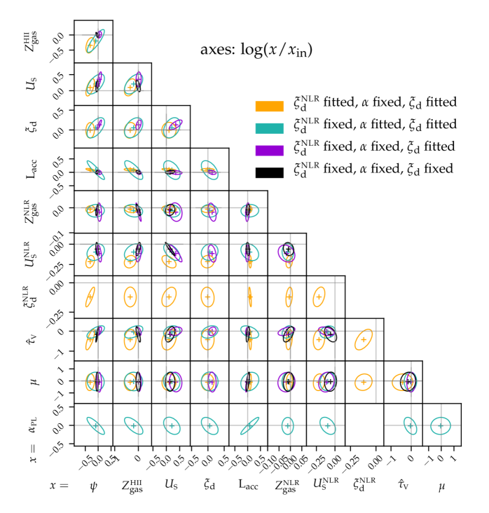
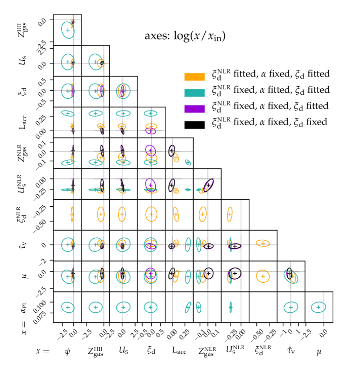
We proceed with the most challenging case of equal contributions of NLR and H ii regions to the H$\beta$ flux. Figs. 6 and 7 show the average joint posteriors for all fitted parameters for the $z=0$ and $z=2$ galaxy, respectively. We display the constraints for different configurations of fitted parameters, as indicated in the legend. Notably, the constraints are quite different for the two different objects. For instance, $\alpha_{\textsc{pl}}$ is well recovered for the $z=0$ object, but is significantly biased for the $z=2$ object. The biased estimates of $\alpha_{\textsc{pl}}$ for the $z=2$ object consequently lead to significantly biased estimates of $\log U_{\textsc{s}}^{\textsc{nlr}}$, $\hbox{$\textnormal{Z}$}_{\textnormal{gas}}^{\textsc{nlr}}$ and $L_{\textnormal{acc}}$. We therefore learn that the accuracy of the $\alpha_{\textsc{pl}}$ estimates depends heavily on the region of the observable parameter space that is being probed. In other words, $\alpha_{\textsc{pl}}$ can be well retrieved for objects in certain regions of the [N ii]$\lambda 6584$ BPT diagram, probably dependent on the sampling of the parameter space by the models and the degeneracies present in that particular region. We therefore suggest that $\alpha_{\textsc{pl}}$ should be fixed as standard when using this set of observables, unless reaching an acceptable fit requires this parameter to be varied.

A parameter which was found to be problematic in the AGN-dominated fits is $\xi_{\textnormal{d}}^{\textsc{nlr}}$(Section 3.3.1), which again is poorly constrained in case of equal contributions by NLR and H ii regions. $\xi_{\textnormal{d}}^{\textsc{nlr}}$ is degenerate with ${\Psi}$, $L_{\textnormal{acc}}$ and $\log U_{\textsc{s}}^{\textsc{nlr}}$, meaning that when $\xi_{\textnormal{d}}^{\textsc{nlr}}$ is un-constrained, the recovery of these parameters will also be biased. Fixing $\xi_{\textnormal{d}}^{\textsc{nlr}}$ somewhat improves the retrieval of the NLR parameters, but for the $z=0$ galaxy, $\xi_{\textnormal{d}}$ is still poorly constrained. This parameter is degenerate with $\log U_{\textsc{s}}$  which is, in turn, degenerate with $\log U_{\textsc{s}}^{\textsc{nlr}}$. Therefore fixing both $\xi_{\textnormal{d}}^{\textsc{nlr}}$ and $\xi_{\textnormal{d}}$ provide less biased estimates of the ionization parameters of the NLR and H ii region emission. We therefore obtain best constraints for both objects when $\xi_{\textnormal{d}}$ and $\xi_{\textnormal{d}}^{\textsc{nlr}}$ are both fixed.

Finally, $\mu$ is well constrained for the $z=0$ object for the different configurations of the fitted and fixed parameters but it is not so well constrained for the same configurations for the $z=2$ object. In order not to be biased by the incertitude on the retrieval of this parameter, we fix the value of $\mu$ in the following sections.

3.4 Influence of S/N on parameter retrieval

Figure 8: Triangle plots of the NLR parameter retrieval for the $z=0$ AGN-dominated objects. Different colors represent different S/N in emission lines. For a given parameter, the axes show the logarithmic fraction of the output by the input value.

Figure 9: Same as Fig. 8 but for the parameter retrieval of the H ii region for SF-dominated objects at $z=0$.

Figure 10: Same as Fig. 8 but for the parameter retrieval of the H ii region and the NLR for objects at $z=0$ with an equal contribution of both regions to H$\beta$.

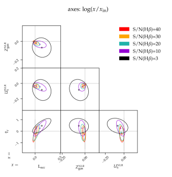
We investigate the S/N in emission lines required to derive un-biased parameter estimates. Based on the results for the $\textrm{S/N(H}\beta)\sim 100$ fits, we fix $\xi_{\textnormal{d}}$, $\xi_{\textnormal{d}}^{\textsc{nlr}}$, $\alpha_{\textsc{pl}}$ and $\mu$. For the AGN-dominated galaxies, the $z=0$ object constraints degrade with S/N more noticeably than for the $z=2$ object, so to be conservative, we only show the $z=0$ results in Fig. 8. These results suggest that the AGN parameters are well-constrained at $\textrm{S/N(H}\beta)\gtrsim 20$. With decreasing S/N, degeneracies between $L_{\textnormal{acc}}$ and $\hat{\tau}_{\textsc{v}}$, as well as $L_{\textnormal{acc}}$ and $\log U_{\textsc{s}}^{\textsc{nlr}}$ become more problematic, causing increasingly biased estimates of the NLR properties. The specific behaviour with low S/N will be different for each object as our results in Section 3 show how dependent parameter retrieval is on the point in parameter space occupied by the object, because of the very non-linear and irregular coverage of the models in observable space.

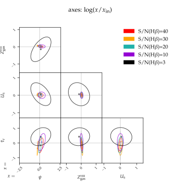
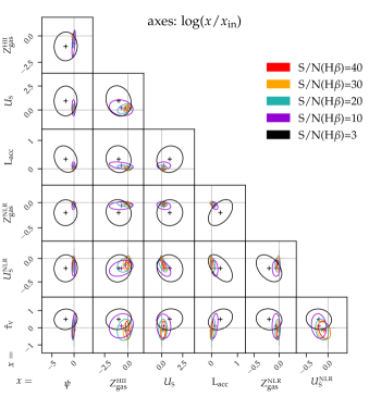
The H ii region properties for the star-formation dominated objects are well constrained and un-biased down to $\textrm{S/N(H}\beta)\sim 10$, as displayed in Fig. 9. Disentangling the contributions from star-forming and NLR components requires higher S/N, however, as illustrated by Fig. 10, which shows the parameter retrieval for the case with equal contributions by SF and NLR to H$\beta$. Parameter retrieval starts to become biased and poorly constrained for $\textrm{S/N(H}\beta)\lesssim 30$.

3.5 NLR contribution to the spectrum

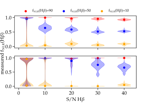
beagle can be used to identify the potential contribution by an AGN to the emission-line luminosities of a galaxy. To test how well beagle can detect the presence of an AGN, we show the retrieved fractional NLR contribution to H$\beta$ flux as a function of the S/N on H$\beta$ in Fig. 11. If we wish only to identify objects with a significant contribution from the NLR to H$\beta$, a S/N of 3 in H$\beta$ is sufficient for our adopted properties of a typical $z=0$ galaxy. However, this S/N is insufficient to reliably estimate the fractional contribution to H$\beta$, which is over-estimated if stars and the AGN contribute in equal amounts to the line flux.

For our $z=2$ galaxy, the fractional contribution of the NLR to H$\beta$ is completely unconstrained at S/N$(\hbox{H$\beta$})=3$. For S/N$(\hbox{H$\beta$})\sim 10$, the NLR contribution is over-estimated for the mixed case. However, only a small probability of a high NLR contribution to the star-formation dominated spectrum (seen from the low fractional area of the yellow curve above 0.5) means that even at this reasonably low S/N, a fairly clean sample of objects with significant contribution of NLR to H$\beta$ flux can selected. Being more conservative, S/N$\sim 20-30$ is required to firmly identify objects with possible NLR contribution, as well as constraining that contribution. It is harder to distinguish NLR contribution in the $z=2$ case because the metallicity is lower, and so key line fluxes such as [O iii]$\lambda 5007$, [O ii]$\lambda 3726,\lambda 3729$ or [O i]$\lambda 6300$ are also much fainter with respect to H$\beta$. This leads to much more overlap between the star-forming and NLR models in this region of the BPT diagram (see Fig. 3), making separation of the NLR and star-forming contributions more challenging. The addition of other line ratios may improve the ability of finding NLR contribution at low metallicity.

Figure 11: Retrieved fractional contribution of the NLR to the total H$\beta$ flux for each object in our simulated grid. The upper (lower) panel shows the retrieval for the typical $z=0$ ($z=2$) objects with different input fractional NLR contribution to H$\beta$ as displayed in the legend.

4 Discussion

Other works have investigated the derivation of NLR physical parameters from emission lines. Throughout the discussion, we compare the modelling assumptions we make to those of other works, with the aim of outlining when and why different models will provide different (or similar) properties for the same data sets. The works we compare to are: the strong-line calibrations of Storchi-Bergmann et al. (1998) and Dors (2021), and the Bayesian approaches of Pérez-Montero et al. (2019) and Thomas et al. (2018b). Before making comparisons, we summarise the different approaches in more detail here.

4.1 Different approaches to deriving NLR physical properties

4.1.1 Storchi-Bergmann et al. 1998

The first calibration of oxygen abundances based on strong optical line emission from NLRs was provided by Storchi-Bergmann et al. (1998). They used cloudy to produce a grid of emission line fluxes for an incident radiation field described by the segmented power-law of Mathews & Ferland (1987) (which is shown in comparison to that used in the F16 models in Fig. 1). The grid covers a range of oxygen abundances and ionization parameters. Although not explicitly stated, the ionization parameter is likely that at the inner edge of the cloud (rather than at the radius of the Strömgrem sphere as for the F16 model grid). They account for both primary and secondary nitrogen, i.e. dependent on the oxygen abundance, following $\log(\textrm{N/O})=0.96[\hbox{$12+\log(\textnormal{O}/\textnormal{H})$}]-9.29$. They also account for depletion of refractory elements from the gas phase onto dust grains following the values of the observed abundance of the interstellar medium from Cowie & Songaila (1986). The following equations describe the two calibrations for the gas-phase oxygen abundance derived by Storchi-Bergmann et al. (1998):

$$\begin{array}[]{l@{}l@{}l}\rm(O/H)_{SB98,1}&=&8.34+(0.212\,x)-(0.012\,x^{2})-(0.002\,y)\\ &+&(0.007\,xy)-(0.002\,x^{2}y)+(6.52\times 10^{-4}\,y^{2})\\ &+&(2.27\times 10^{-4}\,xy^{2})+(8.87\times 10^{-5}\,x^{2}y^{2}),\\ \end{array}$$ (8)

where $x$ = [N ii]$\lambda 6548,\lambda 6584$/H$\alpha$ and $y$ = [O iii]$\lambda 4959,\lambda 5007$/H$\beta$ and

$$\begin{array}[]{lll}(\rm{O/H})_{{\rm SB98,2}}&=&8.643-(0.275\,u)+(0.164\,u^{2})\\ &+&(0.655\,v)-(0.154\,uv)-(0.021\,u^{2}v)\\ &+&(0.288v^{2})+(0.162uv^{2})+(0.0353u^{2}v^{2}),\\ \end{array}$$ (12)

where $u$ = log([O ii]$\lambda 3726,\lambda 3729$/[O iii]$\lambda 4959,\lambda 5007$) and $v$ = log([N ii]$\lambda 6548,\lambda 6584$/H$\alpha$). The term (O/H) above corresponds to 12+log(O/H). Both calibrations are valid for $\rm 8.4\>\leq\>12+log(O/H)\>\leq\>9.4$.

The calibrations are appropriate for $\hbox{$n_{\textsc{h}}$}=300\,\textrm{cm}^{-3}$, but they also provide a correction factor for different densities:

$$(\textrm{O/H})_{final}=(\textrm{O/H})-0.1\,\log(\hbox{$n_{\textsc{h}}$}/300)$$ (13)

4.1.2 Dors 2021

The first strong-line calibration based on gas-phase oxygen abundance estimates derived from the $T_{\textnormal{e}}$ method (or electron temperature method) for NLRs was presented in Dors (2021). From the $T_{\textnormal{e}}$-derived gas-phase oxygen abundances of a sample of AGNs, Dors (2021) provide a 2D surface fitted to the objects within a 3D space defined by $12+\log(\textnormal{O}/\textnormal{H})$, $R_{23}$ and $P$ (defined below):

$$R_{23}=\dfrac{\hbox{[O\,{\sc ii}]$\lambda 3726,\lambda 3729$}+\hbox{[O\,{\sc iii}]$\lambda 4959,\lambda 5007$}}{H\beta}$$ (14)

$$P=\frac{\hbox{[O\,{\sc iii}]$\lambda 4959,\lambda 5007$}/\hbox{H$\beta$}}{R_{23}}$$ (15)

The $R_{23}$ ratio is often used as an oxygen abundance indicator but is known to be dependent on ionization parameter, as well as the hardness of the ionizing radiation (Pilyugin, 2000), while $P$ is sensitive to radiation hardness (Pilyugin, 2001). The resulting calibration is defined as:

$$\hbox{$\hbox{$\textnormal{Z}$}_{\textnormal{gas}}^{\textsc{nlr}}$}=(-1.00\pm 0.09)P+(0.036\pm 0.003)R_{23}+(8.80\pm 0.06)$$ (16)

where $\hbox{$\hbox{$\textnormal{Z}$}_{\textnormal{gas}}^{\textsc{nlr}}$}=12+\log(\rm O/H)$.

The oxygen abundances used to derive the above calibration do still rely on photoionization models, though indirectly. In particular, when only one auroral line is detected (in the case of Dors 2021, the [Oiii]$\lambda 4363$ line), the temperature for part of the nebula is measured, and abundance estimates of the ionization species found within that region is well determined. Yet, to derive the total oxygen abundance, one needs to account for all ionization species that exist in regions with different effective temperatures. The temperature of these other regions must, therefore, be inferred using other methods. Dors et al. (2020b) created a grid of photoionization models to derive the relationship between the temperature of the high ionization region, $t_{3}$ (where oxygen is doubly ionized, traced by [O iii]$\lambda 4959,\lambda 5007$ and [Oiii]$\lambda 4363$), and the low ionization region, $t_{2}$ (where oxygen is singly ionized). To derive a relation between $t_{2}$ and $t_{3}$ suitable for the NLR, Dors et al. (2020b) created a grid of models using ionizing spectra with power-law slopes of $\hbox{$\alpha_{\textsc{pl}}$}=-0.8,-1.1,-1.4$, ionization parameters over the range $-3.5$ to $-0.5$ (again, defined at the inner radius of the ionized cloud), and metallicities over the range $0.2<\hbox{$\hbox{$\textnormal{Z}$}_{\textnormal{gas}}^{\textsc{nlr}}$}/\hbox{$\hbox{$\textnormal{Z}$}_{\odot}$}<2.0$, and for a range of different electron densities from 100 to 3000 cm^-3. In this work, they follow the relation $\log(\textrm{N/O})=1.29[\hbox{$12+\log(\textnormal{O}/\textnormal{H})$}]-11.84$ to assign a given nitrogen abundance. They also fit a relation between $t_{2}$ and $t_{3}$ for the whole grid, as well as for different electron densities. This relation may therefore be reasonable for ‘typical’ NLRs (if the grid presented in Dors et al. (2020b) is appropriate for ‘typical’ NLRs), but individual galaxies will have very different $t_{2}/t_{3}$ values, as demonstrated by the wide spread in $t_{2}/t_{3}$ for their fiducial grid (their figure 5). Treatment of depletion onto dust grains is not referred to in their publications.

4.1.3 Pérez-Montero et al. 2019

Pérez-Montero et al. (2019) extended the Bayesian-like Hii-Chi-mistry code (Pérez-Montero, 2014) to include characterization of the NLR gas using a grid of photoionization models produced with cloudy v.17.01. The incident ionizing radiation consists of two components: that characterizing the ‘big blue bump’ [the curved component peaking at $\log(\nu/\textnormal{Hz})\sim 13.5$ in Fig. 1], and a power-law slope between 2keV (6Å) and 5eV (2500Å) of $\alpha_{\textnormal{ox}}=-0.8$ (they also compare to a model with $\alpha_{\textnormal{ox}}=-1.2$); power-law emission with $\alpha_{x}=-1$ representing the non-thermal X-ray emission. We show the incident radiation in Fig. 1. Pérez-Montero et al. (2019) add dust within the NLR and model the gas as homogeneously-distributed with filling factor 0.1 and hydrogen density, $\hbox{$n_{\textsc{h}}$}=500\,\textrm{cm}^{-3}$. All element abundances are assumed to scale to solar, except for nitrogen, which is an additional free parameter.

Hii-Chi-mistry uses standard line ratios to derive physical parameters, and works by first constraining N/O using the ratios between [N ii]$\lambda 6584$ and [O ii]$\lambda 3726,\lambda 3729$ and between [N ii]$\lambda 6584$ and [S ii]$\lambda 6717,\lambda 6731$, before constraining metallicity and ionization parameter. The chemical composition of the gas is characterized by the total oxygen abundance, which covers the range $6.9<\hbox{$12+\log(\textnormal{O}/\textnormal{H})$}<9.1$, $-2<\log(\textrm{N/O})<0$ and the released version of the code covers $-2.5<\hbox{$\log U_{\textsc{s}}^{\textsc{nlr}}$}<-0.5$. The ionization parameter in these models is defined the same way as for beagle (following description in section 3.1 of Pérez-Montero 2014). The models consider default grain properties and relative abundances, and all elements but Nitrogen are scaled to the solar values given by Asplund et al. (2009) considering the cloudy default depletion factors. Finally, we note that the code is not able to disentangle the contributions of star formation and NLR to the lines.

4.1.4 Thomas et al. 2018

NebularBayes, presented in Thomas et al. (2018a), is the only code, other than beagle, which simultaneously fits the star-forming and NLR contributions to nebular emission. The NLR models are based on physically motivated prescriptions for the incident radiation produced by the accretion disc (Thomas et al., 2016). The accretion disc model has three parameters: the energy of the peak of the accretion disc emission, E_peak; the photon index of the inverse Compton scattered power-law tail, $\Gamma$ (non-thermal X-ray radiation); and the proportion of the total flux that goes into the non-thermal tail, p_NT. The last two parameters are fixed to the fiducial values of $\Gamma=2.0$ and p${}_{NT}=0.15$.

The NLR grid included in NebularBayes is calculated for constant pressure models using mappings v5.1 (Sutherland & Dopita, 2017). This is different from the constant density models produced for the other works. Groves et al. (2004) demonstrated the large difference in coverage of the BPT plane that dusty isobaric models introduce. In particular, for the optical line ratios explored in this paper, their isobaric dusty model curves also better sample the parameter space covered by the data than their dust-free, constant density models. This is due to the absorption of ionizing photons by dust, which increases the radiation pressure (and hence density), especially at high values of the ionization parameter. The four parameters of the NLR that can be derived using NebularBayes are: oxygen abundance of the gas; ionization parameter, $\log U_{\textnormal{in}}^{\textsc{nlr}}$, defined at the inner edge of the ionized gas; peak of the ionizing radiation, $\textnormal{E}_{\textnormal{peak}}$; and pressure.

Thomas et al. (2018b) demonstrates $\textnormal{E}_{\textnormal{peak}}$ cannot be constrained when fitting to [O ii]$\lambda 3726,\lambda 3729$  [N iii]$\lambda 3869$  H$\beta$  [Oiii]$\lambda 4363$  [O iii]$\lambda 4959,\lambda 5007$  [O i]$\lambda 6300$  He i$\lambda 5876$  H$\alpha$  [N ii]$\lambda 6584$  and [S ii]$\lambda 6717,\lambda 6731$ (those available in the SDSS DR7 MPA JHU measured line fluxes), but find that values in the range 40–50 eV give reasonable fractions of NLR contribution, and so fix this parameter to $\hbox{$\textnormal{E}_{\textnormal{peak}}$}=45$ eV.

The grid of models includes 12 oxygen abundances in the range $\rm-1.7\>\leq\>log(O/H)\>\leq\>0.54$, using the oxygen abundance scaling from Nicholls et al. (2017). Depletion onto dust grains is considered based on iron being $97.8\%$ depleted. The ionization parameter at the inner edge of the nebula can take 11 uniformly spaced values in the range $-4.2\leq\hbox{$\log U_{\textnormal{in}}^{\textsc{nlr}}$}\leq-0.2$. The initial gas pressure samples 12 values in the range $4.2\leq\log P/k(\rm cm^{-3}K)\leq 8.6$ and values of $\textnormal{E}_{\textnormal{peak}}$ sample six values in the range $-2.0\leq\log\hbox{$\textnormal{E}_{\textnormal{peak}}$}(\rm keV)\leq-0.75$.

4.2 Comparison to other works and data

Figure 12: Gas-phase oxygen abundance ($12+\log(\textnormal{O}/\textnormal{H})$) versus different emission line ratios, log(R23) (defined in equation 14) and log([O ii]$\lambda 3726,\lambda 3729$/[O iii]$\lambda 4959,\lambda 5007$). In these figures we show the coverage of different NLR emission line models via lines and symbols with a range of metallicity and ionization parameters. The symbols and lines range from fainter to darker colours from lower to higher $\log U_{\textsc{s}}^{\textsc{nlr}}$ or $\log U_{\textnormal{in}}^{\textsc{nlr}}$ respectively, as indicated in the legend. The black, grey and open circles show the measured emission line ratios and inferred NLR $12+\log(\textnormal{O}/\textnormal{H})$ values for a set of type-2 AGNs collated in Dors et al. (2017). Black circles display the $12+\log(\textnormal{O}/\textnormal{H})$ estimates from Dors et al. (2017), while the grey and open circles display the $12+\log(\textnormal{O}/\textnormal{H})$ estimates calculated with the two Storchi-Bergmann et al. (1998) NLR calibrations, defined in equations 8 and 12.

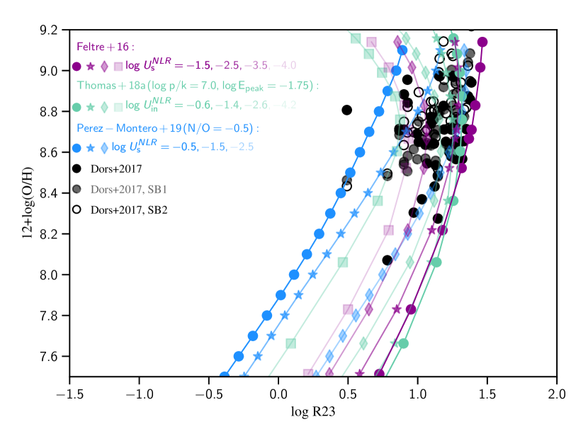
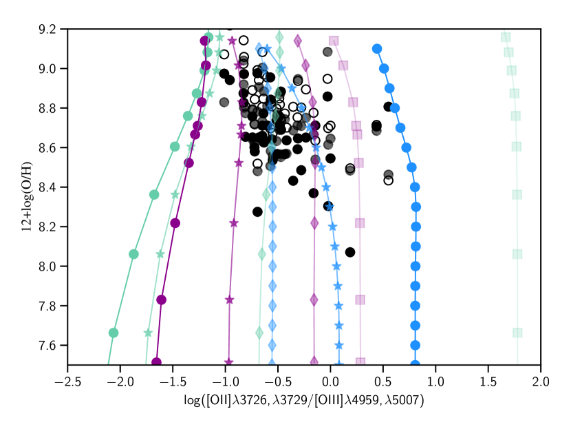
We start by comparing our NLR-emission models (F16) to those of Thomas et al. (2018a) and Pérez-Montero et al. (2019), as well as observed line ratios of 44 observed Seyfert II galaxies collated by Dors et al. (2017). Fig. 12 shows gas-phase $12+\log(\textnormal{O}/\textnormal{H})$ against two different emission line ratios: R₂₃ (defined in equation 14) and $\log(\hbox{[O\,{\sc ii}]$\lambda 3726,\lambda 3729$}/\hbox{[O\,{\sc iii}]$\lambda 4959,\lambda 5007$})$. The lines and matching coloured symbols show the coverage of different models in these plots, while the black and grey symbols show measured line ratios and estimated abundances for the observed galaxies. For each of the observed galaxies, we show three different abundance estimates: those from Dors et al. (2017) (filled black circles) which were estimated by comparing directly to cloudy photoionization models; and those derived with each of the Storchi-Bergmann et al. (1998) calibrations, with filled grey (open black symbols) showing the measurements obtained with the calibration in equation 8 (12). As noted by Storchi-Bergmann et al. (1998), the second calibration (equation 12) leads to systematically higher oxygen abundance estimates than the other two methods.

The models in Fig. 12 span a range of ionization parameters ranging from high to low values with dark-to-faint symbols. For the F16 models, we set $\hbox{$\alpha_{\textsc{pl}}$}=-1.7$. Thomas et al. (2018b) fix E_peak to 45 eV, which is somewhat higher than the peak incident radiation within our models. We investigated values in the range $8<\hbox{$\textnormal{E}_{\textnormal{peak}}$}/\textnormal{eV}<56$ but in order not to crowd the plot too much, we show the results for a central value within this range of $\sim 17.8$ eV. We also explored the full pressure range $4.2<\log(\textnormal{P/k})<8.6$, but plot those with the central value of $\log(\textrm{P/k})=7$. Then, since the Pérez-Montero et al. (2019) model grid encompasses a wide range of N/O abundances, we fix to a value of log(N/O)=$-0.5$ (the same considered as the ‘standard’ one by Pérez-Montero et al. (2019)), although the diagrams in Fig. 12 are not very sensitive to the value chosen.

Fig. 12 (a) shows the oxygen abundance versus R23, which is defined in equation 14. The F16 models cover the full range of the observations, with the exception of a few objects with the lowest values of R23. The Pérez-Montero et al. (2019) models provide good coverage of the observations with low values of R23, but provide only marginal coverage of the highest R23 values. We display the Thomas et al. (2018b) models with a single value of $\textnormal{E}_{\textnormal{peak}}$, although have tested a range from 8 to 56 eV, finding that the models cover the full range of observed values, except for those few observations with the lowest R23. It is important to note that the abundance estimates of the observed objects plotted are not objectively more secure than other abundance estimates presented in this work. They are subject to their own modelling assumptions, so we focus mostly on the coverage of the plotted models over the emission line ratio space.

Fig. 12 (b) shows the gas-phase oxygen abundance for the same models and data as in Fig. 12 (a), but plotted against $\hbox{[O\,{\sc ii}]$\lambda 3726,\lambda 3729$}/\hbox{[O\,{\sc iii}]$\lambda 4959,\lambda 5007$}$. The Thomas et al. (2018a) and Pérez-Montero et al. (2019) models do not include [Oiii]$\lambda 4959$, which we assume to have 1/3 the flux of [O iii]$\lambda 5007$. We see that for the range of ionization parameters plotted, our models cover the parameter space spanned by the observations for all but the highest $\hbox{[O\,{\sc ii}]$\lambda 3726,\lambda 3729$}/\hbox{[O\,{\sc iii}]$\lambda 4959,\lambda 5007$}$ ratios. The Pérez-Montero et al. (2019) models cover the highest $\hbox{[O\,{\sc ii}]$\lambda 3726,\lambda 3729$}/\hbox{[O\,{\sc iii}]$\lambda 4959,\lambda 5007$}$ values, but observations with $\hbox{[O\,{\sc ii}]$\lambda 3726,\lambda 3729$}/\hbox{[O\,{\sc iii}]$\lambda 4959,\lambda 5007$}\lesssim-0.5$ are not covered. The Thomas et al. (2018a) models cover the full range of $\hbox{[O\,{\sc ii}]$\lambda 3726,\lambda 3729$}/\hbox{[O\,{\sc iii}]$\lambda 4959,\lambda 5007$}$ ($\lesssim$-0.5) from the observations.

Both panels of Fig. 12 show that the Pérez-Montero et al. (2019) models give the opposite dependence of R23 and [O ii]$\lambda 3726,\lambda 3729$/[O iii]$\lambda 4959,\lambda 5007$ on $\log U_{\textsc{s}}^{\textsc{nlr}}$ to those of F16 and Thomas et al. (2018a). To understand this, we plot $\log U_{\textsc{s}}^{\textsc{nlr}}$ as a function of [O ii]$\lambda 3726,\lambda 3729$/[O iii]$\lambda 4959,\lambda 5007$ in Fig. 13. Pérez-Montero et al. (2019) chose to publish only the highest $\log U_{\textsc{s}}^{\textsc{nlr}}$ models, as the behaviour between $\log U_{\textsc{s}}^{\textsc{nlr}}$ and [O ii]$\lambda 3726,\lambda 3729$/[O iii]$\lambda 5007$ is double-valued in their models. We do not see the same behaviour in the F16 models with $\hbox{$\alpha_{\textsc{pl}}$}=-1.7$, but when we plot our models with shallower $\hbox{$\alpha_{\textsc{pl}}$}=-1.2$, we start to see a similar behaviour at the highest $\log U_{\textsc{s}}^{\textsc{nlr}}$ and $12+\log(\textnormal{O}/\textnormal{H})$ values (red symbols). The strong increase in [O ii]$\lambda 3726,\lambda 3729$/[O iii]$\lambda 5007$ with $\log U_{\textsc{s}}^{\textsc{nlr}}$ of the Pérez-Montero et al. (2019) models is therefore presumably due to the choice of a hard incident ionizing spectrum (Fig. 1). This is also likely the reason for the moderate offset to higher [O ii]$\lambda 3726,\lambda 3729$/[O iii]$\lambda 5007$ values at given $\log U_{\textsc{s}}^{\textsc{nlr}}$ compared to the F16 models (given that the partially ionized zone will be more extensive).

Figure 13: $\log U_{\textsc{s}}^{\textsc{nlr}}$ or $\log U_{\textnormal{in}}^{\textsc{nlr}}$ versus [O ii]$\lambda 3726,\lambda 3729$/[O iii]$\lambda 4959,\lambda 5007$ for the F16 and Pérez-Montero et al. (2019) models for a range of different $12+\log(\textnormal{O}/\textnormal{H})$ values. We show the F16 models with two values of $\alpha_{\textsc{pl}}$: -1.2 (red) and -1.7 (violet), as indicated in the legend.

Figure 14: The ion fractions of $\rm{H}^{+}$ (black), $\rm{He}^{2+}$ (orange), $\rm{O}^{+}$ (turquoise), $\rm{O}^{2+}$ (sky blue), $\rm{O}^{3+}$ (dark blue) and $\rm{O}^{4+}$ (purple) as a function of the total hydrogen column density. The NLR models have $\hbox{$\hbox{$\textnormal{Z}$}_{\textnormal{gas}}^{\textsc{nlr}}$}=0.030$, $\hbox{$\alpha_{\textsc{pl}}$}=-1.2$ and $\hbox{$\log U_{\textsc{s}}^{\textsc{nlr}}$}=-1.5$ (left) and -2.5 (right).

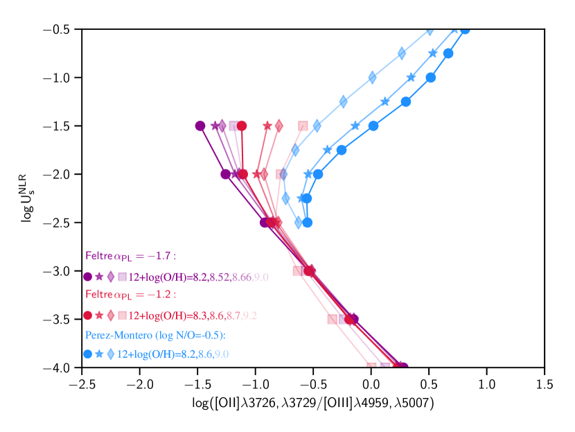
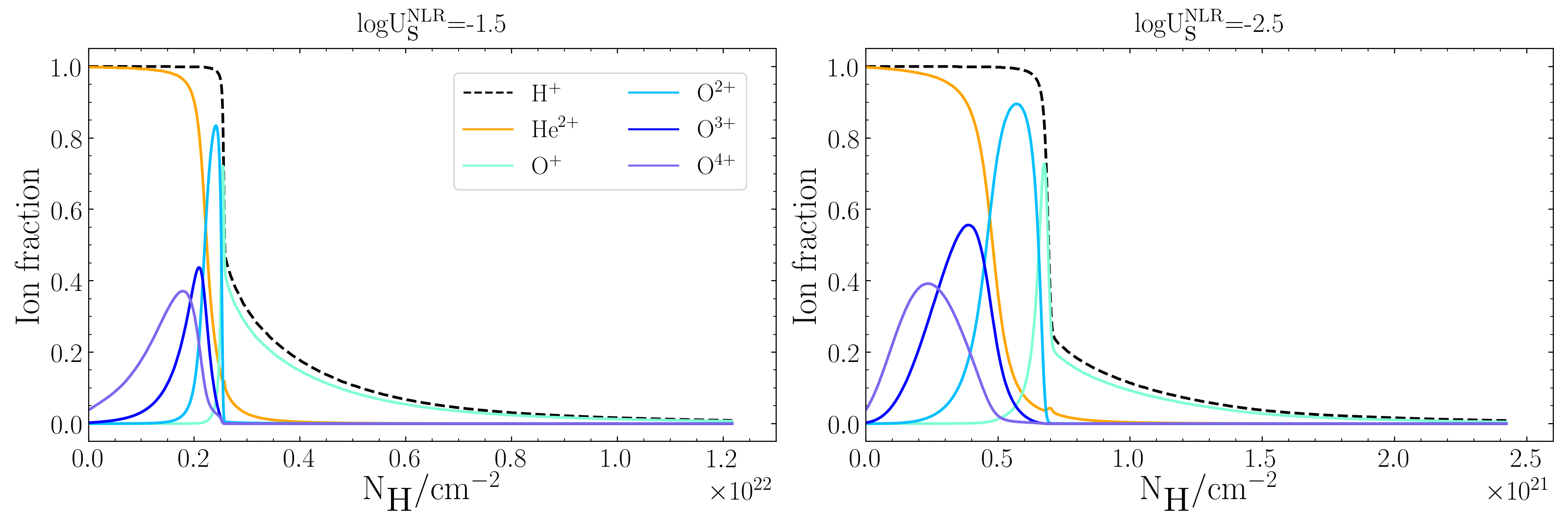
Including only the higher part of the $\log U_{\textsc{s}}^{\textsc{nlr}}$ fork, the Pérez-Montero et al. (2019) models will measure an opposite $12+\log(\textnormal{O}/\textnormal{H})$ versus $\log U_{\textsc{s}}^{\textsc{nlr}}$ to that measured with the Thomas et al. (2018b) or F16 models, which will in turn provide systematically different oxygen abundances. The data used in the Pérez-Montero et al. (2019) fitting could not distinguish which branch of $\log U_{\textsc{s}}^{\textsc{nlr}}$ versus [O ii]$\lambda 3726,\lambda 3729$/[O iii]$\lambda 4959,\lambda 5007$ the data inhabit. It would clearly be beneficial to better constrain the ionization state of NLRs in observed type-2 AGN to motivate the range of $\log U_{\textsc{s}}^{\textsc{nlr}}$ the models must span. Fig. 14 displays the ion fraction for a number of different species (hydrogen, helium and oxygen) from the F16 models with $\hbox{$\alpha_{\textsc{pl}}$}=-1.2$. The ion fraction are shown as a function of the total hydrogen column density, $\rm{N}_{\rm{H}}(R)=\hbox{$n_{\textsc{h}}^{\textsc{nlr}}$}\epsilon R$. The high energy photons from hard ionising radiation of the accretion disc penetrates further through the gas than lower energy photons, creating a partially ionized region. We might expect [O ii]$\lambda 3726,\lambda 3729$/[O iii]$\lambda 5007$ to decrease with increasing $\log U_{\textsc{s}}^{\textsc{nlr}}$. However, as explained in Pérez-Montero et al. (2019), and shown clearly in Fig. 14, for high ionization parameters and hard ionizing radiation, this is not the case as at small radii within the Strömgrem radius, [O iii]$\lambda 5007$ is lost to higher ionization states of oxygen such as $\rm{O}^{3+}$ and $\rm{O}^{4+}$, while $\rm{O}^{+}$ is still present in the partially ionized zone. There are no visible emission lines from these higher ionization states in the wavelength range of SDSS. However, He ii has a similar ionization energy to Oiv (54.4eV versus 54.9eV), and the SDSS spectra provide coverage of the [He ii]$\lambda 4686$ recombination line.

4.3 Nebular [He ii]$\lambda 4686$ fluxes to constrain the ionization state of the NLR in type-2 AGNs within SDSS

We measure the nebular [He ii]$\lambda 4686$ fluxes for 463 confirmed type-2 AGNs presented in Dors et al. (2020a) from DR7 SDSS spectra (Abazajian et al., 2009). [He ii]$\lambda 4686$ is not delivered in the MPA-JHU group distribution of measured line fluxes used in Dors et al. (2020a), since measurements of this line can be complicated by stellar wind features and broadening. We measured [He ii]$\lambda 4686$ using the python package emcee (Foreman-Mackey et al., 2013). Since we wish to gain constraints on the nebular (narrow-line) contribution to the [He ii]$\lambda 4686$ line, we tie the width of the line to the width of [O iii]$\lambda 5007$ in the same spectra, by simultaneously fitting to the two lines. This effectively uses information from the higher S/N [O iii]$\lambda 5007$ line to provide a strong prior on the shape of [He ii]$\lambda 4686$ if it is to arise in the same physical region. We define continuum regions on either side of the two lines and subtract a linear fit to the continuum before performing the line fits. In the case where no obvious nebular [He ii]$\lambda 4686$ emission is present, the tied fitting will provide firm constraints on the limits on the [He ii]$\lambda 4686$ flux with the delivered uncertainties. We report the measured line fluxes and line widths in Table 4.

Table 4: [He ii]$\lambda 4686$ line fluxes measured for the sample of type-2 AGNs presented by Dors et al. (2020a). Full sample will be available online.

MJD-PLATE-FIBER	[He ii]$\lambda 4686$ flux	width
	(/10${}^{-}16$ erg s-1 cm-2)	(/Å)
51882-0442-061	$0.826\pm 0.270$	$2.36\pm 0.04$
52056-0603-545	$0.209\pm 0.145$	$2.03\pm 0.23$
51691-0340-153	$0.258\pm 0.192$	$4.19\pm 0.86$
52079-0631-387	$0.231\pm 0.152$	$1.95\pm 0.05$
52017-0516-232	$1.01\pm 0.26$	$3.03\pm 0.12$
51915-0453-002	$1.17\pm 0.30$	$3.61\pm 0.08$
52049-0618-535	$0.261\pm 0.184$	$3.31\pm 0.23$
52000-0335-428	$0.135\pm 0.116$	$1.83\pm 0.33$

Figure 15: Assessing the ionization state of the gas within the type-2 AGN sample from Dors et al. (2020a). With our measurements of the [He ii]$\lambda 4686$ line from the SDSS spectra of these objects (see text for details), we compare log([O ii]$\lambda 3726,\lambda 3729$/[O iii]$\lambda 4959,\lambda 5007$) versus log([He ii]$\lambda 4686$/[O ii]$\lambda 3726,\lambda 3729$) [log([He ii]$\lambda 4686$/[O iii]$\lambda 4959,\lambda 5007$)] to the F16 models with $\alpha_{\textsc{pl}}$=-1.7 in the left [right] panels. The highest $\log U_{\textsc{s}}^{\textsc{nlr}}$ models have low [O ii]$\lambda 3726,\lambda 3729$/[O iii]$\lambda 4959,\lambda 5007$ ratios. The data shows a clear trend of decreasing [O ii]$\lambda 3726,\lambda 3729$/[O iii]$\lambda 4959,\lambda 5007$ with increasing [He ii]$\lambda 4686$/[O ii]$\lambda 3726,\lambda 3729$ or decreasing [He ii]$\lambda 4686$/[O iii]$\lambda 4959,\lambda 5007$, as shown by the F16 models.

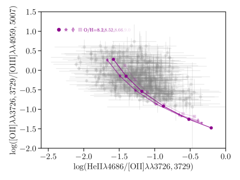
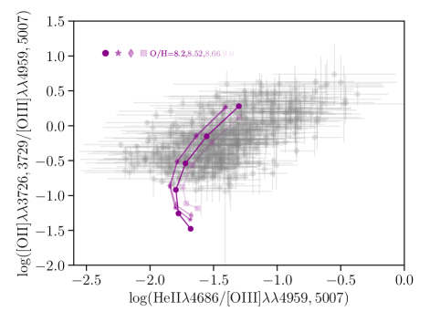
We show [O ii]$\lambda 3726,\lambda 3729$/[O iii]$\lambda 4959,\lambda 5007$ against [He ii]$\lambda 4686$/[O ii]$\lambda 3726,\lambda 3729$ (left) and [He ii]$\lambda 4686$/[O iii]$\lambda 4959,\lambda 5007$ (right) in Fig. 15, with the F16 models for comparison. For this figure, we used the MPA-JHU line fluxes for [O ii]$\lambda 3726,\lambda 3729$ and [O iii]$\lambda 4959,\lambda 5007$. The sample of type-2 AGNs clearly follow the general trend of the F16 models. Unfortunately the models of Pérez-Montero et al. (2019) do not include [He ii]$\lambda 4686$, so we cannot compare to their predicted ratios directly. If [O ii]$\lambda 3726,\lambda 3729$/[O iii]$\lambda 4959,\lambda 5007$ were increasing with $\log U_{\textsc{s}}^{\textsc{nlr}}$ (as for the Pérez-Montero et al. 2019 models in Fig. 13), we would expect [He ii]$\lambda 4686$/[O ii]$\lambda 3726,\lambda 3729$ to increase with [O ii]$\lambda 3726,\lambda 3729$/[O iii]$\lambda 4959,\lambda 5007$, as well as much higher values of [He ii]$\lambda 4686$/[O ii]$\lambda 3726,\lambda 3729$ for the observed galaxies. The observations show low values of [He ii]$\lambda 4686$/[O ii]$\lambda 3726,\lambda 3729$ and a negative trend between [O ii]$\lambda 3726,\lambda 3729$/[O iii]$\lambda 4959,\lambda 5007$ and [He ii]$\lambda 4686$/[O ii]$\lambda 3726,\lambda 3729$ (Fig. 15, a), suggesting that the set of observed type-2 AGNs have significantly lower ionization parameter than covered by the Pérez-Montero et al. (2019) models.

4.4 Comparison of the nitrogen and sulfur emission lines

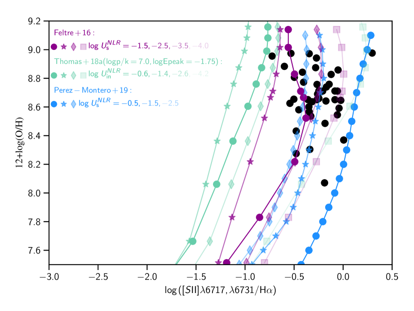
Because the [S ii]$\lambda 6717,\lambda 6731$ doublet is routinely used to derive the gas density in photoionized regions, we have also compared the predictions for this doublet from the different NLR models and data presented in the previous sections. In particular, we show in Fig. 16 the gas-phase oxygen abundance as a function of the ratio [S ii]$\lambda 6717,\lambda 6731$/H$\alpha$. In this case, we only show the data with the predictions for $12+\log(\textnormal{O}/\textnormal{H})$ from Dors et al. 2017 in order to not crowd the figure too much. The Pérez-Montero et al. 2019 models reproduce the data except for the points with the highest oxygen abundances and lowest [S ii]$\lambda 6717,\lambda 6731$/H$\alpha$ ratios. The coverage of the F16 and Thomas et al. 2018a is very similar and almost complete except for three objects with high [S ii]$\lambda 6717,\lambda 6731$/H$\alpha$ ratios. We have noted (not shown here) than for lower values of $\alpha_{\textsc{pl}}$ F16 models cover better this region of the parameter space.

Abundance studies of galactic and extragalactic H ii regions find that nitrogen has a primary origin for the low-metallicity regime ($12+\log(\textnormal{O}/\textnormal{H})$$\lesssim 8.2$) and a secondary one for the high-metallicity regime (e.g. Mouhcine & Contini, 2002; Pérez-Montero & Contini, 2009). Groves et al. 2004 find that the nitrogen abundance from the primary and secondary origin can be related to that of oxygen using an equation of the form Equation 1. To capture the richness of the variation of the N abundance as a function of O, we have expanded the grid of NLR models. The fiducial grid has a N/O dependence on the oxygen abundance following:

$$\rm{log}(\rm{N/O})_{\rm{tot}}\approx\rm{log}\{10^{-1.732}+10^{[\rm{log(O/H)_{\rm{tot}}}+2.19]}\}+C$$ (17)

with $\rm C=-0.25$. Now we are parametrizing N/O in terms of the total abundances, $\rm{(N/O)}_{\rm{tot}}$ (i.e. gas + dust) and its dependence on the total oxygen abundance, $\rm{(O/H)}_{\rm{tot}}$ (gas + dust). In expanding the grid we add two new values of the normalisation, $C$, with $\rm C=0$ (the Nicholls et al. 2017 relation) and $\rm C=0.5$ (the upper limit). See Plat et al. (in prep.) for the details of how these models have been computed.

We test the nitrogen abundance in the different grid of models using the N2 and O3N2 line ratios, defined as follows:

$${\rm N2}=\log\left(\dfrac{\hbox{[N\,{\sc ii}]$\lambda 6584$}}{\hbox{H$\alpha$}}\right)$$ (18)

$${\rm O3N2}=\log\left(\frac{\hbox{[O\,{\sc iii}]$\lambda 5007$}}{\hbox{H$\beta$}}\frac{\hbox{H$\alpha$}}{\hbox{[N\,{\sc ii}]$\lambda 6584$}}\right)$$ (19)

Figure 16: Gas-phase oxygen abundance ($12+\log(\textnormal{O}/\textnormal{H})$) as a function of [S ii]$\lambda 6717,\lambda 6731$/H$\alpha$ for the same models as in Fig. 12.

Figure 17: Gas-phase oxygen abundance ($12+\log(\textnormal{O}/\textnormal{H})$) as a function of N2 (a, see equation 18) and O3N2 (b, see equation 19) for the same models as in Fig. 12 and different variations of the N/O relation: the Gutkin et al. 2016 relation ($\rm C=-0.25$) and the upper limit from eq. 17 ($\rm C=0.5$) for the F16 models and the highest and lowest values for nitrogen abundance of Pérez-Montero et al. 2019 grid. The data points are from Dors et al. 2017.

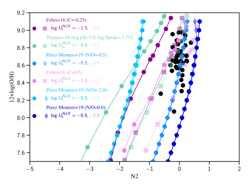
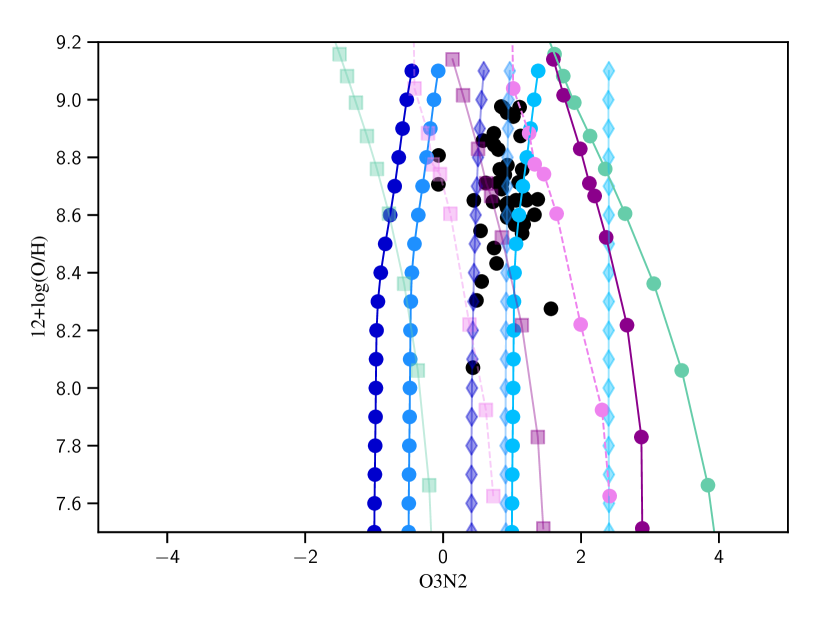
We show in Fig. 17 the gas phase oxygen abundance as a function of these line ratios. For completeness, we show F16 and Pérez-Montero et al. 2019 models with different N/O values. In particular, for the Pérez-Montero et al. 2019 models, we add the ones with the lowest and highest value of N/O (cyan and dark blue points) and for the F16 models, the ones with the highest ($\rm C=0.5$, pink points with dashed lines) and lowest ($\rm C=-0.25$ that of equation 1) scaling factor of the N/O relations explored. We recall that nitrogen abundance is not a free parameter in the Thomas et al. 2018a grid. Most likely due to the fact that nitrogen abundances is fixed, we see in Fig. 17a how Thomas et al. 2018a models are not able to sample the data points with the highest nitrogen abundances. However, increasing the N/O value allows for a full and almost full coverage of the data for Pérez-Montero et al. 2019 and F16 models respectively. In Fig. 17b the three grids of models sample well the space of the diagram where the data lie. We note however, that in the case of Thomas et al. 2018a models, for data points with low O3N2 values, the $\log U_{\textsc{s}}^{\textsc{nlr}}$ parameter might be underestimated. This might be due to the lack of higher Nitrogen abundances that will tend to be compensated in the O3N2 ratio with weaker [O iii]$\lambda 5007$ lines, and therefore, lower $\log U_{\textsc{s}}^{\textsc{nlr}}$ values.

beagle does not yet allow for sampling over N/O, though this comparison to observations shows that it is vital to adequately explain measured line ratios including Nitrogen. It is beyond the scope of this paper to implement and test retrieval of parameters including the new N/O grid with our pedagogical approach, but this functionality will be implemented for future work.

4.5 Comparing to the Dors 2021 $T_{\mathrm{e}}$-based empirical emission-line calibration

Figure 18: Dors (2021) empirical $T_{\textrm{e}}$-based $12+\log(\textnormal{O}/\textnormal{H})$ calibration, shown as the grey surface in $12+\log(\textnormal{O}/\textnormal{H})$–P–R23 space (where P and R23 are defined in Eqs. 15 and 14, respectively). Both panels show a sample of observed AGNs with $12+\log(\textnormal{O}/\textnormal{H})$ estimated from the $T_{\textrm{e}}$ method by Dors (2021) (black points). The F16 models are shown in panel (a) for two values of $\alpha_{\textsc{pl}}$, and for a range of ionization parameters spanning $-4<\hbox{$\log U_{\textsc{s}}^{\textsc{nlr}}$}<-1.5$ with dark-to-light colours spanning high-to-low $\log U_{\textsc{s}}^{\textsc{nlr}}$ values. Panel (b) includes the Thomas et al. (2018a) and Pérez-Montero et al. (2019) models (see text for details). The 3D version of these figures can be found at https://chart-studio.plotly.com/~AlbaVidalGarcia/15/#/.

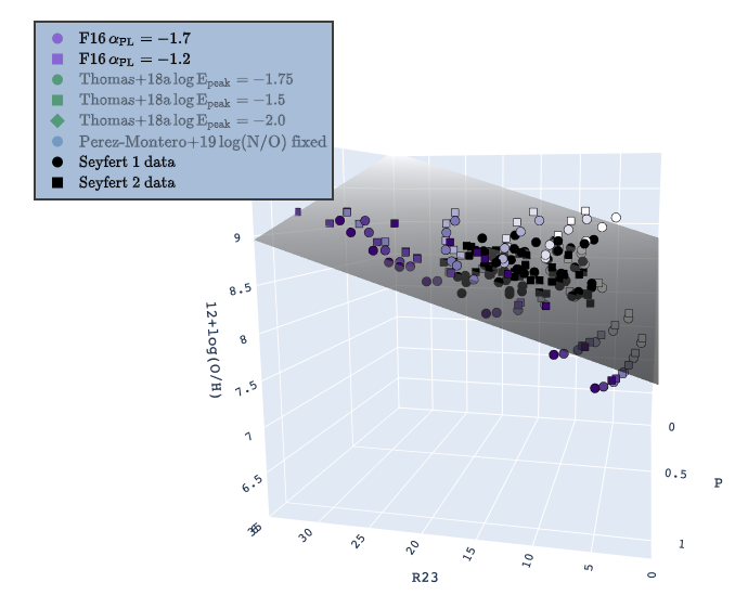
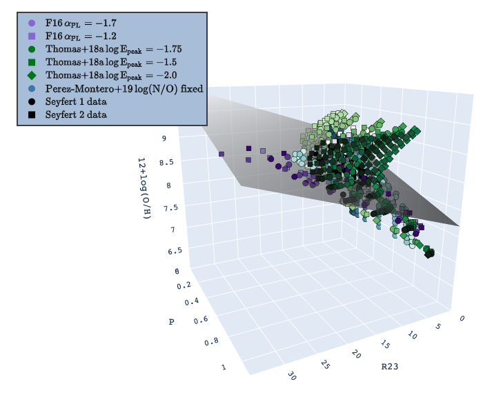
We plot the different theoretical models against the Dors (2021) empirical emission-line calibration in Fig. 18. The calibration describes a surface in $12+\log(\textnormal{O}/\textnormal{H})$–P–R23 space (as described in Eqs. 14 and 15 in Section 4.1.2). This provides a quick comparison of the models to $T_{\mathrm{e}}$-based NLR oxygen-abundance estimates without running full fits with beagle. We will present full beagle fits to SDSS type-2 AGNs in a future paper in this series. The black symbols display the $T_{\mathrm{e}}$-based gas-phase oxygen abundance measurements for the set of AGNs used to produce this empirical calibration, while the grey plane shows the empirical calibration.

Fig. 18 (a) shows the F16 models plotted for a range of $\log U_{\textsc{s}}^{\textsc{nlr}}$, $12+\log(\textnormal{O}/\textnormal{H})$, and two values of $\alpha_{\textsc{pl}}$ ($-1.2$ and $-1.7$). For a given $\alpha_{\textsc{pl}}$ and $12+\log(\textnormal{O}/\textnormal{H})$, different colours represent different $\log U_{\textsc{s}}^{\textsc{nlr}}$ values, with dark-to-light colours spanning high-to-low values. We see that at very low metallicities our models sit below the plane describing the Dors (2021) empirical relation. Within the region occupied by the observed galaxies, the models agree well with the empirical relation until high metallicities, where the models curve up from the empirical plane. The observations also preferentially scatter above the relation. The behaviour of the models suggests this scatter to higher oxygen abundances is real, not simply intrinsic scatter about the empirical plane. Therefore, objects above the relation have higher oxygen abundances than can be explained by their position in the P-R23 plane, while the models can capture this behaviour. This behaviour is also observed in the Thomas et al. (2018a) models (constant pressure models). The curvature from the plane is reminiscent to the effect of the addition of dust in NLR in Groves et al. (2004) as the change from constant density to constant-pressure models. However, our constant density models show a similar behaviour, indicating that the observed curvature might be due to the presence of dust, self consistently modelled in cloudy.

The $\hbox{$\alpha_{\textsc{pl}}$}=-1.7$ models do not cover all the observed data points in Fig. 18 (this might be best appreciated by viewing the interactive plot online, where different models can be removed from the plot for clarity https://chart-studio.plotly.com/~AlbaVidalGarcia/15/#/). A range of $\alpha_{\textsc{pl}}$ appears to be required to fully cover the data. $\hbox{$\alpha_{\textsc{pl}}$}=-1.2$ covers the data well. With our idealized grid exploration in Section 3, we found that the lines chosen for that analysis could not fully constrain $\alpha_{\textsc{pl}}$, and that we recommend the user to set it to $\hbox{$\alpha_{\textsc{pl}}$}=-1.7$ unless there is a significant improvement in the goodness of fit when $\alpha_{\textsc{pl}}$ is allowed to vary. We defer the search of other lines that can constrain better this parameter to a later paper.

Panel (b) of Fig. 18 shows the same models, observations and empirical relation as shown in panel (a), but we include also the Thomas et al. (2018a) and Pérez-Montero et al. (2019) models. In particular, for the Thomas et al. (2018a), we plot a range of $-4.2<\hbox{$\log U_{\textnormal{in}}^{\textsc{nlr}}$}<-0.2$, with dark-to-light colours representing high-to-low values, and for three values of $\textnormal{E}_{\textnormal{peak}}$, as indicated in the legend. In particular, we show the one taken as standard throughout this paper, -1.75 (green points) and a lower and a higher one, -2.0 (green diamonds) and -1.5 (green squares) respectively. For the Pérez-Montero et al. (2019) models, we plot a range of $-2.5<\hbox{$\log U_{\textsc{s}}^{\textsc{nlr}}$}<-0.5$ but we do not vary the N/O values because this variation has a negligible impact on the P and R23 values. This figure shows that all models curve off the empirical relation to high metallicities.

This comparison to the Dors (2021) empirical metallicity calibration shows the limitations of both the empirical diagnostic itself and our models. The empirical diagnostic cannot capture the variation with metallicity above the plane. Our models require a range of $\alpha_{\textsc{pl}}$ to account for the data, a parameter we cannot constrain from the set of line ratios we tested. Our tests in Section 3 further demonstrate how biased other NLR gas parameters become when allowing $\alpha_{\textsc{pl}}$ to vary. However, below the empirical relation (lower metallicities), a region of the parameter space we expect to find at higher redshifts with missions such as JWST, the difference between the two values of $\alpha_{\textsc{pl}}$ is less significant for the F16 models. It is beneficial to use Te-based O abundance estimates, empirical diagnostics, and these types of sophisticated radiative transfer models together to tease out the limitations of each approach. Until $T_{\textrm{e}}$ measurements are possible for large samples of type-2 AGNs at high redshift, the radiative transfer models can capture the evolution in the population more effectively than an empirical calibration based on objects in a small range of metallicities.

5 Summary

In this paper we present the incorporation of the Feltre et al. (2016) NLR models into beagle. This addition allows the mixing of emission from H ii regions with that from the NLR of type-2 AGNs. Dust attenuation is applied self-consistently taking into account the dust within the NLR, H ii regions and the diffuse ISM.

We take a pedagogical approach to defining which parameters of our model (from both H ii and NLR regions) can be constrained by fitting a given set of observables in the optical range. To determine this we work with idealised $z\sim 0$ and $z\sim 2$ galaxy spectra with varying contribution of the NLR to H$\beta$ flux. We fit to a set of line ratios ([O i]$\lambda 6300$/H$\alpha$, [N ii]$\lambda 6584$/H$\alpha$, [S ii]$\lambda 6717,\lambda 6731$/H$\alpha$, [O iii]$\lambda 5007$/H$\beta$, H$\beta$/H$\alpha$, [O i]$\lambda 6300$/[O ii]$\lambda 3726,\lambda 3729$ and [O ii]$\lambda 3726,\lambda 3729$/[O iii]$\lambda 5007$) as well as the H$\alpha$ line flux. We then quantify the S/N required to constrain the parameters of our model for different NLR contributions. Finally, we compare the results of our model with those obtained using previously published methods. The main results are the following:

• With the set of observables used, the retrieval of physical parameters for the AGN dominated spectra with high S/N shows degeneracies between $\xi_{\textnormal{d}}^{\textsc{nlr}}$ and $\log U_{\textsc{s}}^{\textsc{nlr}}$ that lead to an underestimation of $\log U_{\textsc{s}}^{\textsc{nlr}}$ and $\hbox{$\textnormal{Z}$}_{\textnormal{gas}}^{\textsc{nlr}}$ if $\xi_{\textnormal{d}}^{\textsc{nlr}}$ is left as a free parameter. We obtain similar results when adding to the observables a ratio sensitive to the N/O abundance. Allowing $\alpha_{\textsc{pl}}$ to vary leads to an over-estimated retrieval of $L_{\textnormal{acc}}$ while still under-estimating $\hbox{$\textnormal{Z}$}_{\textnormal{gas}}^{\textsc{nlr}}$. We find the best recovery of $L_{\textnormal{acc}}$, $\hbox{$\textnormal{Z}$}_{\textnormal{gas}}^{\textsc{nlr}}$and $\log U_{\textsc{s}}^{\textsc{nlr}}$ when fixing both $\xi_{\textnormal{d}}^{\textsc{nlr}}$ and $\alpha_{\textsc{pl}}$.

• The retrieval of physical parameters for the star-formation dominated spectra is also biased by the nebular $\xi_{\textnormal{d}}$. We find that $\xi_{\textnormal{d}}$ is poorly constrained and when left free leads to an over-estimation of the $\log U_{\textsc{s}}$ and $\hbox{$\textnormal{Z}$}_{\textnormal{gas}}^{\textsc{hii}}$, as well as tighter constraints on the biased estimates.

• We also test the case of equal-contributions of NLR and H ii regions to the H$\beta$ flux. In this case, the accuracy of the $\alpha_{\textsc{pl}}$ parameter depends heavily on the region of the observable parameter space that is being probed, so we suggest that it should be fixed, unless varying it is required to reach an acceptable fit. Both $\xi_{\textnormal{d}}$ and $\xi_{\textnormal{d}}^{\textsc{nlr}}$ are degenerate with several parameters when left free, biasing the recovery of these parameters. We obtain the best constraints for the objects when both $\xi_{\textnormal{d}}$ and $\xi_{\textnormal{d}}^{\textsc{nlr}}$ are fixed.

• We have investigated the S/N in H$\beta$ required to derive un-biased parameter estimates (while fixing $\xi_{\textnormal{d}}$, $\xi_{\textnormal{d}}^{\textsc{nlr}}$ and $\alpha_{\textsc{pl}}$). AGN parameters are well constrained with a $\textrm{S/N(H}\beta)\sim 20$ for the AGN-dominated galaxies. H ii region parameters are well constrained with $\textrm{S/N(H}\beta)\sim 10$ for star-formation dominated galaxies. However, we need a higher $\textrm{S/N(H}\beta)\sim 30$ to disentangle the contributions from star-forming and NLR components when they have similar contributions to H$\beta$ flux.

• We test how well beagle can detect the presence of an AGN by retrieving the fractional contribution of the NLR to the total H$\beta$ flux of a galaxy. For the $z=0$ object, we find that a S/N$\sim$10 already allows for identification of objects that have a significant contribution to the flux, even for the most challenging case of equal contributions to the flux from NLR and H ii regions. For the $z=2$ object, a NLR contribution is detected but overestimated at S/N$\sim$10, though we suggest this is still a reasonable limit for which to find objects with a significant NLR contribution.

• We have compared the predictions of our model to those from different sets of models and data compiled in the literature. These include the models from Thomas et al. (2018a) and Pérez-Montero et al. 2019 and the calibrations to derive gas-phase oxygen abundance from Storchi-Bergmann et al. 1998 and Dors 2021 for the data compiled by these last authors. We find that in general, all the models have a good coverage of the parameter space where the data lie. However, we find an opposite dependence of the Pérez-Montero et al. 2019 models of R23 and [O ii]$\lambda 3726,\lambda 3729$/[O iii]$\lambda 4959,\lambda 5007$ on $\log U_{\textsc{s}}^{\textsc{nlr}}$ with respect to those of F16 and Thomas et al. 2018a. This is presumably due to the choice made in Pérez-Montero et al. 2019 to publish only the highest $\log U_{\textsc{s}}$ models, as the behaviour between $\log U_{\textsc{s}}$ and [O ii]$\lambda 3726,\lambda 3729$/[O iii]$\lambda 4959,\lambda 5007$ is double-valued in their models.

• To constrain the ionization state of NLRs in observed type-2 AGN we measure the [He ii]$\lambda 4686$ recombination line that has a similar ionization energy to Oiv, in 463 confirmed type-2 AGNs from DR7 SDSS spectra. From the comparison to the data we see how the data follow the trend of the F16 models and they suggest that these data have a siginificantly lower ionization parameter values than those covered by the Pérez-Montero et al. 2019 models.

• To better capture the dispersion of the N/H-O/H relation in the data, we create a grid of different scaling factors of this relation that we compare to the data and the same set of models from the literature. Whereas F16 and Pérez-Montero et al. 2019 models sample well the region of the parameter space where the data lies, the fact that Thomas et al. 2018a models fix the Nitrogen abundance might lead to an underestimation of the $\log U_{\textsc{s}}^{\textsc{nlr}}$ parameter when fitting to nitrogen emission lines, because models with extremely low $\log U_{\textsc{s}}^{\textsc{nlr}}$ values are needed to sample the data.

• We also compare the models to the empirical emission-line calibration from Dors 2021. Within the region sampled by observations, the models agree well with the empirical calibration. However, at high metallicities, the models curve up from the plane that the empirical calibration draws in the $12+\log(\textnormal{O}/\textnormal{H})$–P–R23 space. The observations are also scattered preferentially above the plane in the region covered by the models. Therefore, it is likely the models can capture the behavior of the observations that also scatter above the plane. At lower metallicities, the models lie below the Dors 2021 calibration. Additionally, the difference between models with different $\alpha_{\textsc{pl}}$ values is less significant, which will help constraining the gas parameters in galaxies at high redshifts, such as those expected to find with missions such as the JWST. In general, the radiative transfer models can capture the behaviour of objects with different oxygen abundances more effectively than an empirical calibration based on objects with a limited range of metallicities.

This is the first in a series of three papers, that will be followed by a paper on fitting of a sample of type-2 AGNs with beagle, and a study of the extent to which emission from shocks and post-AGB stars may affect our inferences.

Data Availability

The astrophysical data used in this publication is supplied within the paper and the online supplementary materials. The idealised spectra analysed in Section 3 will be shared with reasonable request to the corresponding authors.

Statement of contributions by authors

This is a highly collaborative project led by ECL where every author has had an important contribution. In particular for this paper, AF and ECL incorporated the models into BEAGLE. AVG and AP defined and fitted to the idealised models in Section 3 from the parameters that MH provided from the simulations. AVG worked on the discussion comparing to other models which led to ECL measuring HeII line fluxes in SDSS data and also the need of creating a new N/O grid done by AP and AF. The writing has been done by ECL with the help of AVG, and editing by SC. SC, MH and JC have contributed to the scientific discussions and followed the project from the beginning. If the field of astronomy had the mechanism for assigning multiple first authors (as is done in other fields), AVG, AP and ECL would have been assigned as lead authors. We reflect this with the fact that they are assigned as corresponding authors.

References

- Abazajian et al. (2009) Abazajian K. N., et al., 2009, ApJS, 182, 543
- Agostino et al. (2021) Agostino C. J., et al., 2021, ApJ, 922, 156
- Asplund et al. (2009) Asplund M., Grevesse N., Sauval A. J., Scott P., 2009, ARA&A, 47, 481
- Baldwin et al. (1981) Baldwin J. A., Phillips M. M., Terlevich R., 1981, PASP, 93, 5
- Baskin & Laor (2005) Baskin A., Laor A., 2005, MNRAS, 358, 1043
- Bruzual & Charlot (2003) Bruzual G., Charlot S., 2003, MNRAS, 344, 1000
- Bundy et al. (2015) Bundy K., et al., 2015, ApJ, 798, 7
- Castro et al. (2017) Castro C. S., Dors O. L., Cardaci M. V., Hägele G. F., 2017, MNRAS, 467, 1507
- Charlot & Fall (2000) Charlot S., Fall S. M., 2000, ApJ, 539, 718
- Charlot & Longhetti (2001) Charlot S., Longhetti M., 2001, MNRAS, 323, 887
- Chevallard & Charlot (2016) Chevallard J., Charlot S., 2016, MNRAS, 462, 1415
- Cowie & Songaila (1986) Cowie L. L., Songaila A., 1986, ARA&A, 24, 499
- Crummy et al. (2006) Crummy J., Fabian A. C., Gallo L., Ross R. R., 2006, MNRAS, 365, 1067
- Curtis-Lake et al. (2021) Curtis-Lake E., Chevallard J., Charlot S., Sandles L., 2021, MNRAS, 503, 4855
- Díaz-Francés & Rubio (2013) Díaz-Francés E., Rubio F. J., 2013, Statistical Papers, 54, 309
- Dietrich et al. (2003) Dietrich M., Hamann F., Shields J. C., Constantin A., Heidt J., Jäger K., Vestergaard M., Wagner S. J., 2003, ApJ, 589, 722
- Done et al. (2012) Done C., Davis S. W., Jin C., Blaes O., Ward M., 2012, MNRAS, 420, 1848
- Dors (2021) Dors O. L., 2021, MNRAS, 507, 466
- Dors et al. (2014) Dors O. L., Cardaci M. V., Hägele G. F., Krabbe Â. C., 2014, MNRAS, 443, 1291
- Dors et al. (2015) Dors O. L., Cardaci M. V., Hägele G. F., Rodrigues I., Grebel E. K., Pilyugin L. S., Freitas-Lemes P., Krabbe A. C., 2015, MNRAS, 453, 4102
- Dors et al. (2017) Dors O. L. J., Arellano-Córdova K. Z., Cardaci M. V., Hägele G. F., 2017, MNRAS, 468, L113
- Dors et al. (2020a) Dors O. L., et al., 2020a, MNRAS, 492, 468
- Dors et al. (2020b) Dors O. L., Maiolino R., Cardaci M. V., Hägele G. F., Krabbe A. C., Pérez-Montero E., Armah M., 2020b, MNRAS, 496, 3209
- Feltre et al. (2012) Feltre A., Hatziminaoglou E., Fritz J., Franceschini A., 2012, MNRAS, 426, 120
- Feltre et al. (2016) Feltre A., Charlot S., Gutkin J., 2016, MNRAS, 456, 3354
- Ferland et al. (2013) Ferland G. J., et al., 2013, Rev. Mex. Astron. Astrofis., 49, 137
- Feroz et al. (2009) Feroz F., Hobson M. P., Bridges M., 2009, MNRAS, 398, 1601
- Foreman-Mackey et al. (2013) Foreman-Mackey D., Hogg D. W., Lang D., Goodman J., 2013, PASP, 125, 306
- Groves et al. (2004) Groves B. A., Dopita M. A., Sutherland R. S., 2004, ApJS, 153, 75
- Groves et al. (2006) Groves B., Heckman T., Kauffmann G., 2006, MNRAS, 371, 1559
- Gutkin et al. (2016) Gutkin J., Charlot S., Bruzual G., 2016, MNRAS, 462, 1757
- Haardt & Maraschi (1991) Haardt F., Maraschi L., 1991, ApJ, 380, L51
- Hagen et al. (2007) Hagen N., Kupinski M., Dereniak E. L., 2007, Appl. Opt., 46, 5374
- Hamann & Ferland (1993) Hamann F., Ferland G., 1993, ApJ, 418, 11
- Hirschmann et al. (2017) Hirschmann M., Charlot S., Feltre A., Naab T., Choi E., Ostriker J. P., Somerville R. S., 2017, MNRAS, 472, 2468
- Hirschmann et al. (2019) Hirschmann M., Charlot S., Feltre A., Naab T., Somerville R. S., Choi E., 2019, MNRAS, 487, 333
- Kewley et al. (2019) Kewley L. J., Nicholls D. C., Sutherland R. S., 2019, ARA&A, 57, 511
- Maiolino & Mannucci (2019) Maiolino R., Mannucci F., 2019, A&ARv, 27, 3
- Marinacci et al. (2018) Marinacci F., et al., 2018, MNRAS, 480, 5113
- Mathews & Ferland (1987) Mathews W. G., Ferland G. J., 1987, ApJ, 323, 456
- Matsuoka et al. (2009) Matsuoka K., Nagao T., Maiolino R., Marconi A., Taniguchi Y., 2009, A&A, 503, 721
- Matsuoka et al. (2018) Matsuoka K., Nagao T., Marconi A., Maiolino R., Mannucci F., Cresci G., Terao K., Ikeda H., 2018, A&A, 616, L4
- Mignoli et al. (2019) Mignoli M., et al., 2019, A&A, 626, A9
- Mouhcine & Contini (2002) Mouhcine M., Contini T., 2002, A&A, 389, 106
- Nagao et al. (2006a) Nagao T., Marconi A., Maiolino R., 2006a, A&A, 447, 157
- Nagao et al. (2006b) Nagao T., Maiolino R., Marconi A., 2006b, A&A, 447, 863
- Naiman et al. (2018) Naiman J. P., et al., 2018, MNRAS, 477, 1206
- Nelson et al. (2018) Nelson D., et al., 2018, MNRAS, 475, 624
- Nicholls et al. (2017) Nicholls D. C., Sutherland R. S., Dopita M. A., Kewley L. J., Groves B. A., 2017, MNRAS, 466, 4403
- Osterbrock & Ferland (2006) Osterbrock D. E., Ferland G. J., 2006, Astrophysics of gaseous nebulae and active galactic nuclei
- Pérez-Montero (2014) Pérez-Montero E., 2014, MNRAS, 441, 2663
- Pérez-Montero & Contini (2009) Pérez-Montero E., Contini T., 2009, MNRAS, 398, 949
- Pérez-Montero et al. (2019) Pérez-Montero E., Dors O. L., Vílchez J. M., García-Benito R., Cardaci M. V., Hägele G. F., 2019, MNRAS, 489, 2652
- Pillepich et al. (2018) Pillepich A., et al., 2018, MNRAS, 475, 648
- Pilyugin (2000) Pilyugin L. S., 2000, A&A, 362, 325
- Pilyugin (2001) Pilyugin L. S., 2001, A&A, 369, 594
- Reines & Volonteri (2015) Reines A. E., Volonteri M., 2015, ApJ, 813, 82
- Schartmann et al. (2005) Schartmann M., Meisenheimer K., Camenzind M., Wolf S., Henning T., 2005, A&A, 437, 861
- Shemmer & Netzer (2002) Shemmer O., Netzer H., 2002, ApJ, 567, L19
- Skilling et al. (2006) Skilling J., et al., 2006, Bayesian Analysis, 1, 833
- Springel et al. (2018) Springel V., et al., 2018, MNRAS, 475, 676
- Storchi-Bergmann et al. (1998) Storchi-Bergmann T., Schmitt H. R., Calzetti D., Kinney A. L., 1998, AJ, 115, 909
- Sutherland & Dopita (2017) Sutherland R. S., Dopita M. A., 2017, ApJS, 229, 34
- Thomas et al. (2016) Thomas A. D., Groves B. A., Sutherland R. S., Dopita M. A., Kewley L. J., Jin C., 2016, ApJ, 833, 266
- Thomas et al. (2018a) Thomas A. D., Dopita M. A., Kewley L. J., Groves B. A., Sutherland R. S., Hopkins A. M., Blanc G. A., 2018a, ApJ, 856, 89
- Thomas et al. (2018b) Thomas A. D., Kewley L. J., Dopita M. A., Groves B. A., Hopkins A. M., Sutherland R. S., 2018b, ApJ, 861, L2
- Thomas et al. (2019) Thomas A. D., Kewley L. J., Dopita M. A., Groves B. A., Hopkins A. M., Sutherland R. S., 2019, ApJ, 874, 100
- Tomczak et al. (2014) Tomczak A. R., et al., 2014, ApJ, 783, 85
- Veilleux & Osterbrock (1987) Veilleux S., Osterbrock D. E., 1987, ApJS, 63, 295
- Vidal-García et al. (2017) Vidal-García A., Charlot S., Bruzual G., Hubeny I., 2017, MNRAS, 470, 3532
- York et al. (2000) York D. G., et al., 2000, AJ, 120, 1579
- do Nascimento et al. (2022) do Nascimento J. C., et al., 2022, arXiv e-prints, p. arXiv:2203.08602