Computational Study of p$K_{\rm a}$ shift of Aspartate residue in Thioredoxin: Role of Configurational Sampling and Solvent Model

Abstract

Alchemical free energy calculations are widely used in predicting p$K_{\rm a}$ , and binding free energy calculations in biomolecular systems. These calculations are carried out using either Free Energy Perturbation (FEP) or Thermodynamic Integration (TI). Numerous efforts have been made to improve the accuracy and efficiency of such calculations, especially by boosting conformational sampling. In this paper, we use a technique that enhances the conformational sampling by temperature acceleration of collective variables for alchemical transformations and applies it to the prediction of p$K_{\rm a}$ of the buried Asp₂₆ residue in thioredoxin protein. We discuss the importance of enhanced sampling in the p$K_{\rm a}$ calculations. The effect of the solvent models in the computed p$K_{\rm a}$ values is also presented.

FEP, TI, TI-dAFED, GB

1 Introduction

Molecular dynamics (MD) is widely employed in calculating free energy differences between different molecular conformational states and free energy changes along physio-chemical processes in the condensed phase.^{1, 2, 3, 4, 5} Free energy calculations based on Thermodynamic Integration (TI)⁶ and Free Energy Perturbation (FEP)⁷ have been applied to a wide spectrum of problems in chemistry, and biology^{8, 9, 10, 11}, like drug discovery,^{12, 13, 14, 15, 16} ligand binding in proteins^{17, 18, 19, 20}, identifying protonation states of ionizable residues through pK_a calculations,^{21, 22} conformational free energy differences,^{23, 24, 25} and computing solvation free energies.^{26, 27, 28}. In these methods, free energy differences are calculated by introducing some non-physical intermediate states between two physically relevant states. When applied to condensed matter systems, the predictive power of these methods is affected by the slow convergence in the free energy estimates, mainly due to the drastic environmental changes while moving from one state to the other. Systems get trapped in high-energy metastable states during the simulation resulting in poor conformational sampling.

This issue is addressed by combining the alchemical methods with enhanced sampling MD techniques. Along these lines, FEP/TI combined with umbrella sampling,^{29, 30, 31} TI-driven Adiabatic Free Energy Dynamics (dAFED),^{32, 33} FEP combined with Hamiltonian Replica Exchange Molecular Dynamics,³⁴ FEP combined with solute tempering replica exchange and other global tempering methods^{35, 36, 37, 38}, simulated scaling method for localized enhanced sampling,³⁹ and thermodynamic integration with enhanced sampling (TIES)⁴⁰ were proposed by various authors.

Amongst them, the TI-driven Adiabatic Free Energy Dynamics method is particularly interesting. In this method, TI is done along with an enhanced sampling of collective variables (CVs) in the framework of dAFED in which a set of adiabatically decoupled auxiliary variables are coupled with the CVs. A high temperature of the auxiliary variables is used to enhance the sampling of the CV space. Auxiliary variables are harmonically coupled to the CVs, and for maintaining adiabatic decoupling, auxiliary variables are assigned high masses. The dAFED-based sampling can be further enhanced by biasing all or a subset of collective variables.^{41, 42}

An alternative approach for TI/FEP is the $\lambda$-dynamics method, where the perturbation parameter $\lambda$ is treated as a dynamic variable⁴³. The original version has applied umbrella sampling⁴⁴ on the order parameter $\lambda$. This method is further improved by combining it with enhanced sampling methods like metadynamics⁴⁵, named as $\lambda-$metadynamics⁴⁶. The original $\lambda$-dynamics methodology was implemented for modeling multiple substituents at a single site on a common ligand framework. This technique has been combined with other CV-based biasing techniques, such as Local Elevation Umbrella Sampling.^{47, 48, 49} The improved version of this method, named multi-site $\lambda$-dynamics,^{50, 51, 52} enables multiple substituents at multiple sites on a common ligand core. $\lambda$-dynamics approach has various applications in studying relative protein stability and ligand binding⁵³. In recent years, with the advances in machine learning approaches, active learning protocols have been combined with alchemical methods to screen novel drug candidates.⁵⁴ Single-step FEP techniques like Enveloping Distribution Sampling and variants are also gaining attention.^{55, 56, 57}

The protonation state of ionizable amino acid residues is dictated by their interactions with the rest of the protein environment and the surrounding solvent.⁵⁸ The protonation state of the side chains can influence the structure of the proteins and their functions.⁵⁹ p$K_{\rm a}$ measurements provide valuable information about the protonation states of residues within the protein. Ionizable amino acids buried in the interior of proteins can have a substantial shift in its p$K_{\rm a}$ relative to that in solution. Determining the protonation states of the active site residues is critical for predicting the mechanism of enzymatic reactions. Escherichia coli thioredoxin, a soluble protein with 108 amino acids, is involved in various redox and regulatory activities.⁶⁰ In the active site of the thioredoxin, Asp₂₆ is buried in the hydrophobic core close to the redox-active disulfide residue and is known to play a critical role in the function of thioredoxin. Several computational studies have already reported the values of $\Delta$p$K_{\rm a}$ of Asp₂₆ of the protein and experimental measurement of $\Delta$p$K_{\rm a}$ is available.^{61, 34, 62, 21, 63, 64} A large shift in p$K_{\rm a}$ is reported for this system.^{63, 64} Thus this has been considered to be an ideal system for testing alchemical methods for p$K_{\rm a}$ calculations. Simonson et. al. ²¹ reported a $\Delta\Delta F$, which is the relative protonation free energy of Asp₂₆ residue in protein compared to the isolated Asp residue in water, to be 9.1 $\pm$ 4.1 kcal mol^-1. Later, Meng et. al. ³⁴ used Hamiltonian Replica Exchange Molecular Dynamics combined with free energy perturbation. The authors find that the replica exchange simulations boosted the conformational sampling, and the computed free energy change is in excellent agreement with the experimental data. Ji et. al. ⁶² used polarized protein-specific charges (PPCs) to successfully reproduce the experimental p$K_{\rm a}$ of thioredoxin in explicit solvent TI calculations. Martinez et. al.⁶⁵ have shown that considering different protein conformations and polarization is critical for predicting the experimental p$K_{\rm a}$ shift.

In this paper, the TI-dAFED method is used to compute the p$K_{\rm a}$ shift of Asp₂₆ in Escherichia coli thioredoxin. We aim to probe the effect of boosting the conformational sampling in the p$K_{\rm a}$ shift of Asp₂₆, mainly considering that the residue is located within a hydrophobic core of the thioredoxin protein. Further, solvent molecules can directly interact with the Asp₂₆ residue, making the p$K_{\rm a}$ calculations challenging. Explicit and implicit solvent simulations were performed to validate the results in the different solvent environments.

2 Theory and Method

2.1 Thermodynamic Integration (TI)

In the TI method, potential energy is defined as,

$$U(\mathbf{R},\lambda)=f(\lambda)U_{\rm A}(\mathbf{R})+g(\lambda)U_{\rm B}(\mathbf{R})$$ (1)

where $U_{\rm A}$ and $U_{\rm B}$ are the potential energy functions of the states A and B, respectively, ${\bf R}$ is the set of all atomic coordinates, and $\lambda$ is a parameter such that $\lambda\in[0,1]$. Here, $f(\lambda)$ and $g(\lambda)$ are some functions of $\lambda$ such that $\lambda=0$ corresponds to state A, i.e., $U\equiv U_{\rm A}$, and $\lambda=1$ corresponds to state B. Any value of $\lambda$ between 0 and 1 corresponds to an intermediate state. The free energy derivative with respect to $\lambda$ has the form

$$\left(\frac{\partial F}{\partial\lambda}\right)_{N,V,T}=\left\langle\frac{\partial U}{\partial\lambda}\right\rangle\,$$ (2)

which can then be integrated to compute $\Delta F$:

$$\Delta F=F_{\rm B}-F_{\rm A}=\int_{0}^{1}d\lambda\left\langle\frac{\partial U}{\partial\lambda}\right\rangle_{\lambda}\enspace.$$ (3)

In the above, the brackets $\left<...\right>$ represent ensemble average in the canonical ensemble using the potential $U(\lambda)$. When $f(\lambda)=(1-\lambda)$ and $g(\lambda)=\lambda$, then,

$$\left\langle\frac{\partial U}{\partial\lambda}\right\rangle_{\lambda}=\left\langle U_{B}-U_{A}\right\rangle_{\lambda}\enspace.$$ (4)

In our calculations, only the electrostatic potential is changed while going from Asp₂₆-H to Asp${}_{26}^{-}$ with the change of $\lambda$ from 0 to 1.

2.2 Thermodynamic Integration Driven-Adiabatic Free Energy Dynamics (TI-dAFED)

In Temperature Accelerated Molecular Dynamics (TAMD)⁶⁶ and in d-AFED³², an extended Lagrangian is used:^{1, 67}

$$\mathcal{L}_{\rm TAMD/d-AFED}(\mathbf{R},\dot{\mathbf{R}},\mathbf{z},\dot{\mathbf{z}})=\mathcal{L}_{0}(\mathbf{R},\dot{\mathbf{R}})+\sum_{\alpha=1}^{n}\frac{1}{2}\mu_{\alpha}\dot{\mathbf{z}}_{\alpha}^{2}-\sum_{\alpha=1}^{n}\frac{k_{\alpha}}{2}(q_{\alpha}(\mathbf{R})-z_{\alpha})^{2}\enspace$$

where $\mathcal{L}_{0}(\mathbf{R},\dot{\mathbf{R}})$ is the original Lagrangian of the system, $n$ is the number of CVs, $\mu_{\alpha}$ is the mass of the auxiliary degrees of variables $\left\{z_{\alpha}\right\}$, and $k_{\alpha}$ is the coupling constant which determines the strength of the coupling between $\left\{z_{\alpha}\right\}$ and the CVs $\left\{q_{\alpha}\right\}$. The temperature of the auxiliary variables is kept much higher than the physical degrees of freedom. This is achieved by coupling two different thermostats to these degrees of freedom. The masses, $\left\{\mu_{\alpha}\right\}$, are taken much higher than the atomic masses to maintain an adiabatic decoupling between the auxiliary and the physical degrees of freedom. The high temperature of the auxiliary variables boosts the sampling of the CVs, which in turn helps the system to explore the phase space efficiently.

In TI-dAFED simulations,³³ the Lagrangian $\mathcal{L}_{0}$ is composed of the potential energy $U(\mathbf{R},\lambda)$ as given in Eqn. 1. This allows us to enhance the exploration of the CV space while performing the TI simulations. Appropriate reweighting factors are required to recover the free energy differences, as shown below:

$$\Delta F=\int_{0}^{1}d\lambda\,\int d\mathbf{z}\,\,\left<\frac{\partial U}{\partial\lambda}\right>(\mathbf{z};\lambda)\,\,A_{\lambda}(\mathbf{z})\enspace,$$ (5)

where

$$A_{\lambda}(\mathbf{z})=\frac{\exp\left[-\beta{\phi}(\mathbf{z})\right]}{\int d\mathbf{z}\exp\left[-\beta{\phi}(\mathbf{z})\right]}\enspace,$$ (6)

and

$$\phi(\mathbf{z})=-\frac{1}{\beta_{z}}\ln P(\mathbf{z})\enspace.$$ (7)

Here, $P(\mathbf{z})$ is the probability distribution of auxiliary variables at temperature $T_{z}$. The temperature of the auxiliary variables $T_{z}$ is much higher than the physical temperature $T$, and $\beta_{z}=(k_{\rm B}T_{z})^{-1}$ and $\beta=(k_{\rm B}T)^{-1}$, where $k_{\rm B}$ is the Boltzmann constant. The reweighting factors $A_{\lambda}(\mathbf{z})$ are computed by a post-processing script on the bins created within the CV space. In Eqn. 5, we require $\left<\frac{\partial U}{\partial\lambda}\right>(\mathbf{z})$ on the same CV-bins, which in turn is computed by binning the $\left(\frac{\partial U}{\partial\lambda}\right)(t)$ from the simulations, followed by local averaging on every bin.

2.3 pK_a Shift Calculations

Figure 1: Alchemical transformations involved in the calculation of p$K_{\rm a}$ shifts ($\Delta$p$K_{\rm a}$ ) of Asp in thioredoxin are given. The first transformation shows the deprotonation of Asp residue in the protein environment, while the second transformation shows the deprotonation of Asp in water. $\Delta F$ values computed for these two alchemical transformations are used to compute the shift in $\Delta F$, i.e., $\Delta\Delta F$, which in turn is used to compute $\Delta$p$K_{\rm a}$ .

p$K_{\rm a}$ shift of aspartic acid (Asp) residue in the oxidized form of thioredoxin is computed using $\Delta\Delta F$, which is the difference in free energy change for converting Protein-AspH to Protein-Asp$-$ ($\Delta F_{\rm prot}$) and free energy change for converting AspH to Asp$-$ ($\Delta F_{\rm model}$) in solution (Figure 1):

$$\Delta\mathrm{p}K_{\rm a} = \mathrm{p}K_{\rm a}\,(\mathrm{prot})-\mathrm{p}K_{\rm a}\,(\mathrm{model})$$ (8)

$$= \frac{1}{2.303\,k_{B}T}\left[\Delta F_{\mathrm{prot}}-\Delta F_{\mathrm{model}}\right]$$

$$= \frac{1}{2.303\,k_{B}T}\Delta\Delta F$$

Conversion of protonated Asp to deprotonated Asp is an alchemical change, as the proton disappears during this transformation. Such transformations are performed in solvated protein and ligand systems using TI and TI-dAFED methods.

2.4 Computational Setup

Asp model system was constructed using 2N-acetyl-1N-methyl-aspartic acid-1-amide. The protein structure was constructed from the PDB ID:2TRX.⁶⁸ Protonation states of the residues except for Asp₂₆ of the protein were set for pH=7.5. N_δ and N_ϵ of His₆ is taken in the protonated state. All calculations are done in the CUDA-enabled AMBER-18 PMEMD software ^{69, 70, 71, 72} patched with PLUMED 2.6.1.⁷³ The AMBER ff99SB force-field ⁷⁴ is used for all the simulations. The SHAKE algorithm⁷⁵ is used to constrain the covalent bonds with H-atoms. The Langevin thermostat, as available in AMBER-18, was used to control the temperature of the system at 300 K.

We have considered $\lambda=0$ as Asp₂₆-H (protonated) state and $\lambda=1$ as Asp${}_{26}^{-}$ (deprotonated) state. Partial charges for protonated and deprotonated states are taken from the earlier work. ²¹ As $g(\lambda)$ and $f(\lambda)$ are linear functions of $\lambda$, intermediate states are obtained by linearly interpolating the potential energy function. We took 12 $\lambda$ points from 0.0 to 1.0, with a gap of 0.1 and an extra point at 0.05.

We performed implicit and explicit solvent MD simulations. Explicit water simulations are performed with TIP3P⁷⁶ and TIP4P⁷⁷ water models. The initial box size for the explicit solvent simulations was 55$\times$60$\times$62ų and 32$\times$34$\times$29ų while simulating the solvated protein and the solvated model systems, respectively. The protein and the model systems contained 4783 (4697) and 670 (662) water molecules, respectively, while using the TIP3P (TIP4P) force field. The Onufriev, Bashford, and Case generalized Born implicit solvent approach ⁷⁸ was used for the implicit solvent simulations. No counter-charges were present while doing the implicit solvent calculations.

For the case of explicit solvent simulations, we ran 2 ns of $NPT$ ensemble simulations until the density of the system was equilibrated. We performed 20 ns of $NVT$ equilibration for both implicit and explicit solvent models and all the $\lambda$ windows. Starting structure for all other $\lambda$ values was taken from the equilibrated structure of the preceding $\lambda$ simulation. The production runs were for 100 ns for all the $\lambda$ windows. Particle Mesh Ewald method ⁷⁹ is used for calculating long-range interactions in all the explicit solvent simulations. The frictional coefficient for the Langevin thermostat was taken to be 1 $\mathrm{ps}^{-1}$, and a time-step of 1 fs was used. In the case of implicit solvent, the frictional coefficient for Langevin dynamics was taken as 5 $\mathrm{ps}^{-1}$, and 2 fs time-step was used. Berendsen barostat was used for the $NPT$ simulations⁸⁰. The trapezoidal method was used for the numerical integrations concerning TI calculations.

Figure 2: Snapshots showing two conformational states of Asp₂₆ in the protein. The CV $\chi_{2}$ is labeled, and the two distances used as CVs are indicated by dotted lines. Atom colors: C (black), O (red), N (blue), H (white).

Three collective variables were used to enhance various orientations of Asp₂₆ in protein at different values of $\lambda$ (see Figure 2): (1) $\chi_{2}$ dihedral of Asp₂₆, (2) $d[\mathrm{Asp}_{26}\,\mathrm{O}_{\delta 1}-\mathrm{Lys}_{57}\,\mathrm{N}_{\zeta}]$, and (3) $d[\mathrm{Asp}_{26}\,\mathrm{O}_{\delta 2}-\mathrm{Lys}_{57}\,\mathrm{N}_{\zeta}]$. While the first CV enhances the rotation about the dihedral $\chi_{2}$, the second, as well as the third CVs, boost formation and breakage of hydrogen-bonding interactions with Lys₅₇. Real collective variables were coupled with extended CVs by a restraining potential with a spring constant of $1.2\times 10^{3}$ kcal mol^-1 rad^-2 for $\chi_{2}$ dihedral CV, $2.4\times 10^{3}$ kcal mol^-1nm^-2 for the other two CVs. The masses for the three auxiliary variables were 50 a.m.u. Å² $\rm rad^{-2}$, 266 a.m.u., and 266 a.m.u., respectively. The auxiliary variables coupled to the CVs were thermostatted to 1200 K using a Langevin thermostat. It was found that the above parameters were sufficient to obtain a slow diffusion of the auxiliary variables $\{z_{\alpha}\}$ with respect to real-coordinates $\{q_{\alpha}\}$, and that $\{q_{\alpha}\}$ follows $\{z_{\alpha}\}$. The average temperature of the auxiliary variables and the physical variables remained close to the target temperature.

3 Results and Discussions

3.1 Implicit Solvent Simulation

Table 1: Computed $\Delta F_{\rm prot}$, $\Delta F_{\rm model}$, and $\Delta\Delta F$ using various methods and literature data are listed. The free energy values are in kcal/mol. All simulations were carried out for 100 ns per window.

Method	$\Delta F_{\rm prot}$	$\Delta F_{\rm model}$	$\Delta\Delta F=\Delta F_{\rm prot}-\Delta F_{\rm model}$
TI/Implicit	-56.7 $\pm$ 0.9	-62.0 $\pm$ 0.3	5.3 $\pm$ 0.9
TI-dAFED/Implicit	-56.7 $\pm$ 1.0	-62.2 $\pm$ 0.5	5.5 $\pm$ 1.1
TI/TIP3P	-66.9 $\pm$ 2.8	-75.1 $\pm$ 2.8	8.2 $\pm$ 4.0
TI-dAFED/TIP3P	-66.2 $\pm$ 3.1	-74.5 $\pm$ 2.9	8.3 $\pm$ 4.2
TI/TIP4P	-70.9 $\pm$ 2.7	-81.3 $\pm$ 2.9	10.4 $\pm$ 4.0
TI-dAFED/TIP4P	-70.7 $\pm$ 3.2	-80.6 $\pm$ 3.0	9.9 $\pm$ 4.4
Literature data: Ref.21a	-66.0 $\pm$ 3.9	-75.1 $\pm$ 1.1	9.1 $\pm$ 4.1
Literature data: Ref.34b	-54.27 $\pm$ 0.22	-59.68 $\pm$ 0.08	5.41 $\pm$ 0.23
Experiment63			4.8

^a Conventional TI/Explicit: Ref. ^21
b FEP+H-REMD/Implicit: Ref. ³⁴

At first, we are presenting the data of TI calculations using the implicit solvent model. The free energy differences $\Delta F$ were calculated for protein and model as discussed in Section 2 of the manuscript. To check the convergence of the free energy estimate, we monitored $\Delta F$ as a function of simulation time (Figure 3). In the case of the model and the protein, $\Delta F$ has converged within 100 ns per $\lambda$ window. Table 1 has the converged values of $\Delta F_{\rm prot}$, $\Delta F_{\rm model}$, and $\Delta\Delta F$. The same set of calculations was repeated using the TI-dAFED. The results of both conventional TI and TI-dAFED are in excellent agreement with the experimental⁶³ value and the previous simulation data using an implicit solvent.³⁴ From Figure 3, one may conclude that TI-dAFED has better convergence than TI; however, these differences were not substantial considering the error in the estimates. For conventional TI calculations, $\Delta F_{\rm prot}$ converges at about 30 ns/window, whereas TI-dAFED runs give converged $\Delta F_{\rm prot}$ estimate in 5 ns/window itself. It is noted in passing that, TI-dAFED has no additional computational cost compared to a conventional TI simulation.

The convergence is examined in a more detailed manner by calculating the convergence of the derivative of free energy with respect to $\lambda$. Figure 4 shows that the derivative of free energy is also well converged using both methods after 100 ns/window. However, it is clear that TI-dAFED converges faster than TI for protein.

Since we are using linear functions of $\lambda$ for $g(\lambda)$ and $f(\lambda)$, and that the electrostatic potential energy terms of Asp₂₆ is only varied with $\lambda$, $\left<\partial U/\partial\lambda\right>$ has contributions only due to the electrostatic potential arising from the Asp₂₆. Thus $\left<\partial U/\partial\lambda\right>$ is ideally expected to decrease linearly with the increase in $\lambda$ from 0 to 1.^{81, 21} Interestingly, a linear behavior of $\left<dU/d\lambda\right>$ was not found in the case of TI for both protein and model systems, while they are nearly linear in the case of TI-dAFED simulations (Figure 5).

Figure 3: Convergence of $\Delta F$ in simulations using the implicit sol model for the (A) protein and the (B) model system. Results of TI-dAFED (blue) and TI (red) are presented. Error bars are also shown.

Figure 4: Convergence of $\left<\partial U/\partial\lambda\right>$ as a function of $\lambda$ for (A) protein using TI-dAFED method, (B) protein using TI method, (C) model using TI-dAFED method and, (D) model using TI method.

Figure 5: $\left<\partial U/\partial\lambda\right>$ as a function of $\lambda$ for (A) protein and (B) model. The TI-dAFED results are in blue and while the TI results are in red. Error bars are shown as transparent thick lines.

Figure 6: Scatter plot along $\chi_{2}$ and $\emph{d}\,[\mathrm{Asp}_{26}\,\mathrm{O}_{\delta 1}-\mathrm{Lys}_{57}\,\mathrm{N}_{\zeta}$] (A) and $\chi_{2}$ and $\emph{d}\,[\mathrm{Asp}_{26}\,\mathrm{O}_{\delta 2}-\mathrm{Lys}_{57}\,\mathrm{N}_{\zeta}$] (B) with implicit solvent for $\lambda$ equals 0.0, 0.5, and 1.0. The red and the blue colors show the TI and the TI-dAFED results, respectively.

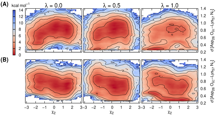
Figure 7: Free energy surface computed along $\chi_{2}$ and $\emph{d}\,[\mathrm{Asp}_{26}\,\mathrm{O}_{\delta 1}-\mathrm{Lys}_{57}\,\mathrm{N}_{\zeta}$] (A) and $\chi_{2}$ and $\emph{d}\,[\mathrm{Asp}_{26}\,\mathrm{O}_{\delta 2}-\mathrm{Lys}_{57}\,\mathrm{N}_{\zeta}$] (B) from TI-dAFED simulations with implicit solvent for $\lambda$ values of 0.0, 0.5, and 1.0. Contours are drawn at 2 kcal mol^-1.

To understand these differences, we compare the conformational sampling achieved in TI and TI-dAFED simulations. Scatter plots of the CV values in Figure 6 are illustrative in this respect. Projected energy surface along the CVs for a few values of $\lambda$ are also presented in Figure 7. Clearly, stable basins on the free energy surfaces are visited in TI and TI-dAFED simulations. However, within the simulation time of 100 ns, TI-dAFED simulations sample a much broader CV space than TI for all the $\lambda$ values.

3.2 Explicit Solvent Simulations

The $\Delta\Delta F$ values were also computed for explicit water using TIP3P water model. The results for the free energy differences are summarized in Table 1. The $\Delta\Delta F$ for TI-dAFED agrees with TI results. However, it is 2.8 kcal mol^-1 higher than that computed using the implicit solvent model and 3.5 kcal mol^-1 higher than the experimental result. Of great interest, an earlier simulation using explicit solvent by Simonson et. al. ²¹ also reported a higher $\Delta\Delta F$ compared to the experimental value.

The convergence of $\Delta F$ and $\left<\partial U/\partial\lambda\right>$ is shown in Figure 8 and Figure 10. Both the quantities are well converged within the error bars in both TI and TI-dAFED simulations. The $\left<\partial U/\partial\lambda\right>$ values for TI and TI-dAFED are also comparable with each other and show a linear trend with the change of $\lambda$ (see Figure 9).

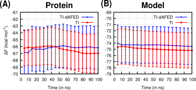
Figure 8: Convergence of $\Delta F$ in simulations using the TIP3P water model for the (A) protein and the (B) model system. Results of TI-dAFED (blue) and TI (red) are presented. Error bars are also shown.

Figure 9: $\left<\partial U/\partial\lambda\right>$ as a function of $\lambda$ for (A) protein and (B) model. The TI-dAFED results are in blue and while the TI results are in red. Error bars are shown as transparent thick lines.

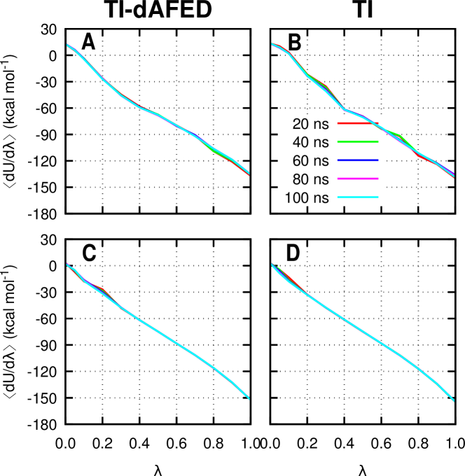
Figure 10: Convergence of $\left<\partial U/\partial\lambda\right>$ as a function of $\lambda$ for (A) protein using TI-dAFED method, (B) protein using TI method, (C) model using TI-dAFED method and, (D) model using TI method. In these simulations, the TIP3P water model was used.

Like in the case of implicit solvent, we find that the conformational sampling in TI-dAFED simulation is significantly higher than TI (Figure 11 and 12), although all the minima are still sampled in TI.

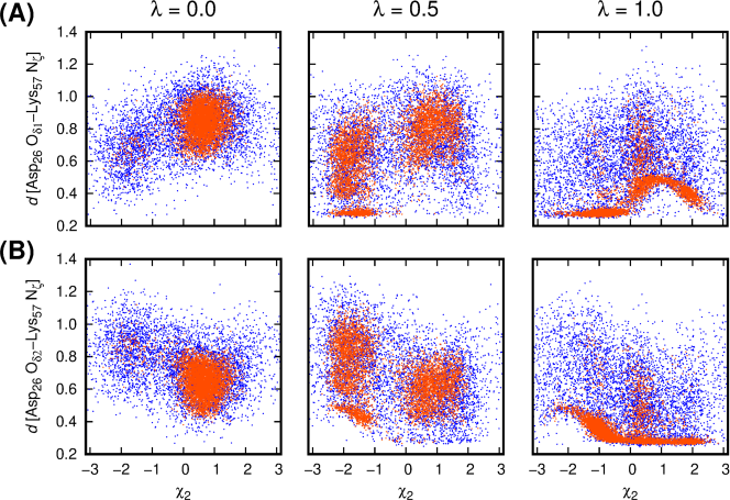
Figure 11: Scatter plot along $\chi_{2}$ and $\emph{d}\,[\mathrm{Asp}_{26}\,\mathrm{O}_{\delta 1}-\mathrm{Lys}_{57}\,\mathrm{N}_{\zeta}$] (A) and $\chi_{2}$ and $\emph{d}\,[\mathrm{Asp}_{26}\,\mathrm{O}_{\delta 2}-\mathrm{Lys}_{57}\,\mathrm{N}_{\zeta}$] coordinates (B) with TIP3P water model for $\lambda$ equals 0.0, 0.5, and 1.0. The red and the blue colors show the TI and the TI-dAFED results, respectively.

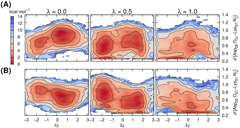
Figure 12: Free energy surface computed along $\chi_{2}$ and $\emph{d}\,[\mathrm{Asp}_{26}\,\mathrm{O}_{\delta 1}-\mathrm{Lys}_{57}\,\mathrm{N}_{\zeta}$] (A) and $\chi_{2}$ and $\emph{d}\,[\mathrm{Asp}_{26}\,\mathrm{O}_{\delta 2}-\mathrm{Lys}_{57}\,\mathrm{N}_{\zeta}$] (B) from TI-dAFED simulations with TIP3P water model, for $\lambda$ equals 0.0, 0.5, and 1.0. Contours are drawn at 2 kcal mol^-1.

To probe the reason for higher $\Delta\Delta F$ while using TIP3P solvent, we have repeated these calculations using the TIP4P water model. The results for the free energy differences are summarized in Table 1. We found that $\Delta\Delta F$ for TI-dAFED is only 0.5 kcal mol^-1 lesser than TI results; see also SI Figures 1-5.

Thus we conclude that the water model is affecting $\Delta\Delta F$ estimate. This could be because non-polarizable TIP3P and TIP4P models may not be able to mimic the correct behavior of water molecules in the hydrophobic pocket in the vicinity of Asp₂₆. As pointed out in the earlier works^{62, 82} a polarized force field might be necessary.

4 Conclusion

TI calculations were performed to compute $\Delta$p$K_{\rm a}$ of Aps₂₆ in thioredoxin protein. We reported the performance of TI-dAFED method for computing $\Delta$p$K_{\rm a}$ . It has been found that TI-dAFED can sample the conformational space exhaustively compared to conventional TI simulations. This aids in quick convergence of $\left<\partial U/\partial\lambda\right>$ and $\Delta F$.

The predicted value of $\Delta\Delta F$ of Aps₂₆ in thioredoxin protein is in excellent agreement with the experimental data when a continuum solvent is used. Contrarily, TIP3P and TIP4P water models are unable to provide a good quantitative prediction of $\Delta\Delta F$, although the direction of the shift is correctly reproduced. The differences in the $\Delta\Delta F$ between TIP3P explicit solvent simulations and the experimental data are within the error. We have found that the quantitative difference in the results is not due to the poor sampling of conformational space when an explicit solvent is taken. Our results point out that a polarized water model may be required to capture the response of the changing electrostatic field around Asp₂₆ along with the change in $\lambda$, in agreement with the earlier findings.^{62, 82}

The authors thank Prof. M. E. Tuckerman (New York University), Adrian E. Roitberg (The University of Florida), Dr. Michel A. Cuendet (Lausanne University Hospital), and Dr. Suman Chakrabarty (S. N. Bose National Centre for Basic Sciences) for fruitful discussions. The support of the Science and Engineering Research Board (India) under the Core Research Grant (Project No: CRG/2019/001276) is gratefully acknowledged. A part of the computational resources was provided by the PARAM Sanganak supercomputing facility under the National Supercomputing Mission at IIT Kanpur. SV thank INSPIRE (Department of Science and Technology) and IIT Kanpur for her Ph.D. fellowship.

The Supporting Information is available free of charge at https://pubs.acs.org/doi/xxx. Various plots from the protein and the model-ligand simulations using TIP4P water model are shown: (i) convergence of $\Delta F$, (ii) $\left<\partial U/\partial\lambda\right>$ as a function of $\lambda$, (iii) convergence of $\left<\partial U/\partial\lambda\right>$ as a function of simulation length, (iv) scatter plot of CVs for different values of $\lambda$, and (v) free energy surfaces along the CV space for different $\lambda$ values.

References

- ME. 2010 ME., T. Statistical mechanics: Theory and molecular simulation; 1st ed. Oxford: Oxford University Press, 2010
- Straatsma and McCammon 1992 Straatsma, T. P.; McCammon, J. A. Computational Alchemy. Annu. Rev. Phys. Chem 1992, 43, 407–435
- Hansen and van Gunsteren 2014 Hansen, N.; van Gunsteren, W. F. Practical Aspects of Free-Energy Calculations: A Review. J. Chem. Theory Comput. 2014, 10, 2632–2647
- Beveridge and DiCapua 1989 Beveridge, D. L.; DiCapua, F. M. Free Energy Via Molecular Simulation: Applications to Chemical and Biomolecular Systems. Ann. Rev. Biophys. Biophys. Chem. 1989, 18, 431–492
- Frenkel and Smit 2002 Frenkel, D.; Smit, B. Understanding Molecular Simulation: From Algorithm to Application, 2nd ed.; Academic Press: San Diego, California, 2002
- Kirkwood 1935 Kirkwood, J. G. Statistical Mechanics of Fluid Mixtures. J. Chem. Phys. 1935, 3, 300–313
- Zwanzig 1954 Zwanzig, R. W. High‐Temperature Equation of State by a Perturbation Method. I. Nonpolar Gases. J. Chem. Phys. 1954, 22, 1420–1426
- Kollman 1993 Kollman, P. Free energy calculations: Applications to chemical and biochemical phenomena. Chem. Rev. 1993, 93, 2395–2417
- Chipot and Pohorille 2007 Chipot, C.; Pohorille, A. Free Energy Calculations: Theory and Applications in Chemistry and Biology; Springer Series in Chemical Physics; Springer Berlin Heidelberg, 2007
- Christ et al. 2010 Christ, C. D.; Mark, A. E.; van Gunsteren, W. F. Basic ingredients of free energy calculations: A review. J. Comput. Chem. 2010, 31, 1569–1582
- Hage et al. 2018 Hage, K. E.; Mondal, P.; Meuwly, M. Free energy simulations for protein ligand binding and stability. Molecular Simulation 2018, 44, 1044–1061
- Abel et al. 2017 Abel, R.; Wang, L.; Harder, E. D.; Berne, B. J.; Friesner, R. A. Advancing Drug Discovery through Enhanced Free Energy Calculations. Acc. Chem. Res. 2017, 50, 1625–1632
- Cournia et al. 2017 Cournia, Z.; Allen, B.; Sherman, W. Relative Binding Free Energy Calculations in Drug Discovery: Recent Advances and Practical Considerations. J. Chem. Inf. Model. 2017, 57, 2911–2937
- Mobley and Klimovich 2012 Mobley, D. L.; Klimovich, P. V. Perspective: Alchemical free energy calculations for drug discovery. J. Chem. Phys. 2012, 137, 230901
- Chodera et al. 2011 Chodera, J. D.; D. L. Mobley, M. R. S.; Dixon, R. W.; Branson, K.; Pande, V. S. Alchemical free energy methods for drug discovery: progress and challenges. Curr. Opin. Struct. Biol. 2011, 21, 150 – 160
- Song and Merz 2020 Song, L. F.; Merz, K. M. Evolution of Alchemical Free Energy Methods in Drug Discovery. J. Chem. Inf. Model. 2020, 60, 5308–5318
- Simonson et al. 2002 Simonson, T.; Archontis, G.; Karplus, M. Free Energy Simulations Come of Age: Protein-Ligand Recognition. Acc. Chem. Res. 2002, 35, 430–437
- Gumbart et al. 2013 Gumbart, J. C.; Roux, B.; Chipot, C. Standard Binding Free Energies from Computer Simulations: What Is the Best Strategy? J. Chem. Theory Comput. 2013, 9, 794–802
- Mobley and Gilson 2017 Mobley, D. L.; Gilson, M. K. Predicting Binding Free Energies: Frontiers and Benchmarks. Annu. Rev. Biophys. 2017, 46, 531–558
- Panday and Ghosh 2019 Panday, S. K.; Ghosh, I. Challenges and Advances in Computational Chemistry and Physics; Springer International Publishing, 2019; pp 109–175
- Simonson et al. 2004 Simonson, T.; Carlsson, J.; Case, D. A. Proton Binding to Proteins: pKa Calculations with Explicit and Implicit Solvent Models. J. Am. Chem. Soc. 2004, 126, 4167–4180
- Jorgensen and Thomas 2008 Jorgensen, W.; Thomas, L. Perspective on Free-Energy Perturbation Calculations for Chemical Equilibria. J. Chem. Theory Comput. 2008, 4, 869–876
- Straatsma and McCammon 1989 Straatsma, T. P.; McCammon, J. A. Treatment of rotational isomers in free energy evaluations. Analysis of the evaluation of free energy differences by molecular dynamics simulations of systems with rotational isomeric states. J. Chem. Phys. 1989, 90, 3300–3304
- Cuendet et al. 2018 Cuendet, M. A.; Margul, D. T.; Schneider, E.; Vogt-Maranto, L.; Tuckerman, M. E. Endpoint-restricted adiabatic free energy dynamics approach for the exploration of biomolecular conformational equilibria. J. Chem. Phys. 2018, 149, 072316
- He et al. 2018 He, P.; Zhang, B. W.; Arasteh, S.; Wang, L.; Abel, R.; Levy, R. M. Conformational Free Energy Changes via an Alchemical Path without Reaction Coordinates. J. Phys. Chem. Lett. 2018, 9, 4428–4435
- Klimovich and Mobley 2010 Klimovich, P. V.; Mobley, D. L. Predicting hydration free energies using all-atom molecular dynamics simulations and multiple starting conformations. J. Comput. Aided Mol. Des. 2010, 24, 307–16
- Procacci 2019 Procacci, P. Solvation free energies via alchemical simulations: let’s get honest about sampling, once more. Phys. Chem. Chem. Phys. 2019, 21, 13826–13834
- Deng et al. 2015 Deng, N.; Zhang, B. W.; Levy, R. M. Connecting Free Energy Surfaces in Implicit and Explicit Solvent: An Efficient Method To Compute Conformational and Solvation Free Energies. J. Chem. Theory Comput. 2015, 11, 2868–2878
- Souaille and Roux 2001 Souaille, M.; Roux, B. Extension to the weighted histogram analysis method: combining umbrella sampling with free energy calculations. Comput. Phys. Commun. 2001, 135, 40–57
- Ngo 2021 Ngo, S. T. Estimating the ligand-binding affinity via -dependent umbrella sampling simulations. J. Comput. Chem. 2021, 42, 117–123
- Leitgeb et al. 2005 Leitgeb, M.; Schröder, C.; Boresch, S. Alchemical free energy calculations and multiple conformational substates. J. Chem. Phys. 2005, 122, 084109
- Abrams and Tuckerman 2008 Abrams, J. B.; Tuckerman, M. E. Efficient and Direct Generation of Multidimensional Free Energy Surfaces via Adiabatic Dynamics without Coordinate Transformations. J. Phys. Chem. B 2008, 112, 15742–15757
- Cuendet and Tuckerman 2012 Cuendet, M. A.; Tuckerman, M. E. Alchemical Free Energy Differences in Flexible Molecules from Thermodynamic Integration or Free Energy Perturbation Combined with Driven Adiabatic Dynamics. J. Chem. Theory Comput. 2012, 8, 3504–3512
- Meng et al. 2011 Meng, Y.; Sabri Dashti, D.; Roitberg, A. E. Computing Alchemical Free Energy Differences with Hamiltonian Replica Exchange Molecular Dynamics (H-REMD) Simulations. J. Chem. Theory Comput. 2011, 7, 2721–2727
- Khavrutskii and Wallqvist 2010 Khavrutskii, I. V.; Wallqvist, A. Computing Relative Free Energies of Solvation Using Single Reference Thermodynamic Integration Augmented with Hamiltonian Replica Exchange. J. Chem. Theory Comput. 2010, 6, 3427–3441
- Wang et al. 2015 Wang, L. et al. Accurate and Reliable Prediction of Relative Ligand Binding Potency in Prospective Drug Discovery by Way of a Modern Free-Energy Calculation Protocol and Force Field. J. Am. Chem. Soc. 2015, 137, 2695–2703
- Jiang et al. 2018 Jiang, W.; Thirman, J.; Jo, S.; Roux, B. Reduced Free Energy Perturbation/Hamiltonian Replica Exchange Molecular Dynamics Method with Unbiased Alchemical Thermodynamic Axis. J. Phys. Chem. B 2018, 122, 9435–9442
- Wang et al. 2019 Wang, L.; Chambers, J.; Abel, R. Methods in Molecular Biology; Springer New York, 2019; pp 201–232
- Li et al. 2007 Li, H.; Fajer, M.; Yang, W. Simulated scaling method for localized enhanced sampling and simultaneous “alchemical” free energy simulations: A general method for molecular mechanical, quantum mechanical, and quantum mechanical/molecular mechanical simulations. J. Chem. Phys. 2007, 126, 024106
- Bhati et al. 2017 Bhati, A. P.; Wan, S.; Wright, D. W.; Coveney, P. V. Rapid, Accurate, Precise, and Reliable Relative Free Energy Prediction Using Ensemble Based Thermodynamic Integration. J. Chem. Theory Comput. 2017, 13, 210–222
- Chen et al. 2012 Chen, M.; Cuendet, M. A.; Tuckerman, M. E. Heating and flooding: A unified approach for rapid generation of free energy surfaces. J. Chem. Phys. 2012, 137, 024102
- Awasthi and Nair 2017 Awasthi, S.; Nair, N. N. Exploring high dimensional free energy landscapes: Temperature accelerated sliced sampling. J. Chem. Phys. 2017, 146, 094108
- Kong and Brooks 1996 Kong, X.; Brooks, C. L. ‐dynamics: A new approach to free energy calculations. J. Chem. Phys. 1996, 105, 2414–2423
- Torrie 1974 Torrie, J. P., Glenn M.; Valleau Monte Carlo free energy estimates using non-Boltzmann sampling: Application to the sub-critical Lennard-Jones fluid. Chem. Phys. Lett. 1974, 28, 578–581
- Laio and Parrinello 2002 Laio, A.; Parrinello, M. Escaping free-energy minima. Proc. Natl. Acad. Sci. 2002, 99, 12562–12566
- Wu et al. 2011 Wu, P.; Hu, X.; Yang, W. -Metadynamics Approach To Compute Absolute Solvation Free Energy. J. Phys. Chem. Lett. 2011, 2, 2099–2103
- Bieler et al. 2014 Bieler, N. S.; Häuselmann, R.; Hünenberger, P. H. Local Elevation Umbrella Sampling Applied to the Calculation of Alchemical Free-Energy Changes via -Dynamics: The -LEUS Scheme. J. Chem. Theory Comput. 2014, 10, 3006–3022
- Bieler and Hünenberger 2015 Bieler, N. S.; Hünenberger, P. H. Orthogonal sampling in free-energy calculations of residue mutations in a tripeptide: TI versus -LEUS. J. Comput. Chem. 2015, 36, 1686–1697
- Hahn et al. 2020 Hahn, D. F.; König, G.; Hünenberger, P. H. Overcoming Orthogonal Barriers in Alchemical Free Energy Calculations: On the Relative Merits of -Variations, -Extrapolations, and Biasing. J. Chem. Theory Comput. 2020, 16, 1630–1645
- Knight and Brooks 2011 Knight, J. L.; Brooks, C. L. I. Multisite Dynamics for Simulated Structure–Activity Relationship Studies. J. Chem. Theory Comput. 2011, 7, 2728–2739
- Hayes et al. 2017 Hayes, R. L.; Armacost, K. A.; Vilseck, J. Z.; Brooks, C. L. Adaptive Landscape Flattening Accelerates Sampling of Alchemical Space in Multisite Dynamics. J. Phys. Chem. B 2017, 121, 3626–3635
- Hayes et al. 2022 Hayes, R. L.; Vilseck, J. Z.; Brooks, C. L. I. Addressing Intersite Coupling Unlocks Large Combinatorial Chemical Spaces for Alchemical Free Energy Methods. J. Chem. Theory Comput. 2022, 18, 2114–2123
- Knight and Brooks III 2009 Knight, J. L.; Brooks III, C. L. -Dynamics free energy simulation methods. J. Comput. Chem. 2009, 30, 1692–1700
- Khalak et al. 2022 Khalak, Y.; Tresadern, G.; Hahn, D. F.; de Groot, B. L.; Gapsys, V. Chemical Space Exploration with Active Learning and Alchemical Free Energies. J. Chem. Theory Comput. 2022, 18, 6259–6270
- Han 1992 Han, K.-K. A new Monte Carlo method for estimating free energy and chemical potential. Phys. Lett. A 1992, 165, 28–32
- Perthold et al. 2020 Perthold, J. W.; Petrov, D.; Oostenbrink, C. Toward Automated Free Energy Calculation with Accelerated Enveloping Distribution Sampling (A-EDS). J. Chem. Inf. Model. 2020, 60, 5395–5406
- König et al. 2021 König, G.; Ries, B.; Hünenberger, P. H.; Riniker, S. Efficient Alchemical Intermediate States in Free Energy Calculations Using -Enveloping Distribution Sampling. J. Chem. Theory Comput. 2021, 17, 5805–5815
- Isom et al. 2010 Isom, D. G.; Castañeda, C. A.; Cannon, B. R.; Velu, P. D.; E., B. G.-M. Charges in the hydrophobic interior of proteins. Proc. Natl. Acad. Sci. 2010, 107, 16096–16100
- Aghera et al. 2012 Aghera, N.; Dasgupta, I.; Udgaonkar, J. B. A Buried Ionizable Residue Destabilizes the Native State and the Transition State in the Folding of Monellin. Biochemistry 2012, 51, 9058–9066
- Holmgren et al. 1975 Holmgren, A.; Söderberg, B. O.; Eklund, H.; Brändén, C. I. Three-dimensional structure of Escherichia coli thioredoxin-S2 to 2.8 A resolution. Proc. Natl. Acad. Sci. 1975, 72, 2305–2309
- Sun et al. 2017 Sun, Z.; Wang, X.; Song, J. Extensive Assessment of Various Computational Methods for Aspartate’s p Shift. J. Chem. Inf. Model. 2017, 57, 1621–1639
- Ji et al. 2008 Ji, C.; Mei, Y.; Zhang, J. Z. Developing Polarized Protein-Specific Charges for Protein Dynamics: MD Free Energy Calculation of pKa Shifts for Asp26/Asp20 in Thioredoxin. Biopys. J. 2008, 95, 1080–1088
- Langsetmo et al. 1991 Langsetmo, K.; Fuchs, J. A.; Woodward, C. The conserved, buried aspartic acid in oxidized Escherichia coli thioredoxin has a pKa of 7.5. Its titration produces a related shift in global stability. Biochemistry 1991, 30, 7603–7609
- Dyson et al. 1991 Dyson, H. J.; Tennant, L. L.; Holmgren, A. Proton-transfer effects in the active-site region of Escherichia coli thioredoxin using two-dimensional proton NMR. Biochemistry 1991, 30, 4262–4268
- Gomez and Vöhringer-Martinez 2019 Gomez, A.; Vöhringer-Martinez, E. Conformational sampling and polarization of Asp26 in pKa calculations of thioredoxin. Proteins: Struct., Funct., Genet. 2019, 87, 467–477
- Maragliano and Vanden-Eijnden 2006 Maragliano, L.; Vanden-Eijnden, E. A temperature accelerated method for sampling free energy and determining reaction pathways in rare events simulations. Chem. Phys. Lett. 2006, 426, 168 – 175
- Awasthi and Nair 2018 Awasthi, S.; Nair, N. N. Exploring high-dimensional free energy landscapes of chemical reactions. WIREs Computational Molecular Science 2018, 9
- Katti et al. 1990 Katti, S. K.; LeMaster, D. M.; Eklund, H. Crystal structure of thioredoxin from Escherichia coli at 1.68 Å resolution. J. Mol. Biol. 1990, 212, 167–184
- Case et al. 2018 Case, D. A. et al. AMBER 18; University of California, San Francisco, 2018
- Salomon-Ferrer et al. 2013 Salomon-Ferrer, R.; Götz, A. W.; Poole, D.; Le Grand, S.; Walker, R. C. Routine Microsecond Molecular Dynamics Simulations with AMBER on GPUs. 2. Explicit Solvent Particle Mesh Ewald. J. Chem. Theory Comput. 2013, 9, 3878–3888
- Mermelstein et al. 2018 Mermelstein, D. J.; Lin, C.; Nelson, G.; Kretsch, R.; McCammon, J. A.; Walker, R. C. Fast and flexible gpu accelerated binding free energy calculations within the amber molecular dynamics package. J. Comput. Chem. 2018, 39, 1354–1358
- Lee et al. 2017 Lee, T.-S.; Hu, Y.; Sherborne, B.; Guo, Z.; York, D. M. Toward Fast and Accurate Binding Affinity Prediction with pmemdGTI: An Efficient Implementation of GPU-Accelerated Thermodynamic Integration. J. Chem. Theory Comput. 2017, 13, 3077–3084
- Tribello et al. 2014 Tribello, G. A.; Bonomi, M.; Branduardi, D.; Camilloni, C.; Bussi, G. PLUMED 2: New feathers for an old bird. Comput. Phys. Commun. 2014, 185, 604 – 613
- Hornak et al. 2006 Hornak, V.; Abel, R.; Okur, A.; Strockbine, B.; Roitberg, A.; Simmerling, C. Comparison of multiple Amber force fields and development of improved protein backbone parameters. Proteins: Struct., Funct., Genet. 2006, 65, 712–725
- Ryckaert et al. 1977 Ryckaert, J.-P.; Ciccotti, G.; Berendsen, H. J. Numerical integration of the cartesian equations of motion of a system with constraints: molecular dynamics of n-alkanes. J. Comput. Phys. 1977, 23, 327–341
- MacKerell et al. 1998 MacKerell, A. D. et al. All-Atom Empirical Potential for Molecular Modeling and Dynamics Studies of Proteins. J. Phys. Chem. B 1998, 102, 3586–3616
- Jorgensen et al. 1983 Jorgensen, W. L.; Chandrasekhar, J.; Madura, J. D.; Impey, R. W.; Klein, M. L. Comparison of simple potential functions for simulating liquid water. J. Chem. Phys. 1983, 79, 926–935
- Onufriev et al. 2002 Onufriev, A.; Case, D. A.; Bashford, D. Effective Born radii in the generalized Born approximation: The importance of being perfect. J. Comput. Chem. 2002, 23, 1297–1304
- Sagui and Darden 1999 Sagui, C.; Darden, T. A. MOLECULAR DYNAMICS SIMULATIONS OF BIOMOLECULES: Long-Range Electrostatic Effects. Annu. Rev. Biophys. Biomol. Struct. 1999, 28, 155–179
- Berendsen et al. 1984 Berendsen, H. J. C.; Postma, J. P. M.; van Gunsteren, W. F.; DiNola, A.; Haak, J. R. Molecular dynamics with coupling to an external bath. J. Chem. Phys. 1984, 81, 3684–3690
- Simonson 2002 Simonson, T. Gaussian fluctuations and linear response in an electron transfer protein. Proc. Natl. Acad. Sci. 2002, 99, 6544–6549
- Burger et al. 2013 Burger, S. K.; Schofield, J.; Ayers, P. W. Quantum Mechanics/Molecular Mechanics Restrained Electrostatic Potential Fitting. J. Phys. Chem. B 2013, 117, 14960–14966