Joint modeling of wind speed and wind direction through a conditional approach

Abstract

Atmospheric near surface wind speed and wind direction play an important role in many applications, ranging from air quality modeling, building design, wind turbine placement to climate change research. It is therefore crucial to accurately estimate the joint probability distribution of wind speed and direction. In this work we develop a conditional approach to model these two variables, where the joint distribution is decomposed into the product of the marginal distribution of wind direction and the conditional distribution of wind speed given wind direction. To accommodate the circular nature of wind direction a von Mises mixture model is used; the conditional wind speed distribution is modeled as a directional dependent Weibull distribution via a two-stage estimation procedure, consisting of a directional binned Weibull parameter estimation, followed by a harmonic regression to estimate the dependence of the Weibull parameters on wind direction. A Monte Carlo simulation study indicates that our method outperforms an alternative method that uses periodic spline quantile regression in terms of estimation efficiency. We illustrate our method by using the output from a regional climate model to investigate how the joint distribution of wind speed and direction may change under some future climate scenarios. Our method indicates significant changes in the variation of wind speed with respect to some directions.

Keywords— Wind speed and direction, conditional approach, Weibull, von Mises, periodic quantile regression

1 Introduction

The atmospheric wind vector plays a significant role in many fields: air-quality monitoring (Zannetti, 2013); wind building engineering (Chen, 2006; Mendis et al., 2007; Holmes and Bekele, 2013); wildfires (Westerling et al., 2004), just to name a few. In clean energy production, wind speed and wind direction play an important role in designing the layout of the wind farm such that the power the wind farm produces is optimal (Carta et al., 2008; Hering and Genton, 2010; Stanley et al., 2020). Consequently, accurate modeling of the probability distribution of wind vector is critical in characterizing its variation.

Wind vector can be represented in either the Cartesian coordinates $(u,v)$ (also known as zonal and meridional velocities) or the polar coordinates $(r,\phi)$, i.e. wind speed and wind direction. Transforming from the Cartesian coordinates to polar coordinates (or vice versa) is achieved using the formula: $(u,v)=(r\sin\phi,\,r\cos\phi)$ (or $(r,\phi)=(\sqrt{u^{2}+v^{2}},\arctan\left(\frac{u}{v}\right))$; due to meteorological convention, the $\arctan$ function is often replaced by the $\text{atan}2$ function). Fig. 1 depicts these two representations of the wind vector using 10-minute wind data measured at 10 meters above ground at the Cabauw Experimental Site for Atmospheric Research (CESAR) tower (KNMI, 2013) over the course of one year during the month of January.

An approach for the empirical modeling of the wind vector is through the joint distribution of $(u,v)$, denoted by brackets $[U,V]$ (Smith, 1971; McWilliams and Sprevak, 1979; Weber, 1997; Reich and Fuentes, 2007; Bessac et al., 2016), where, for example, a bivariate normal distribution can be used (Smith, 1971; McWilliams and Sprevak, 1979; Weber, 1997). However, as indicated in Fig. 1(a), modeling $[V]$ (and $[U]$) using a normal distribution may not be appropriate. Copula approach (Joe, 1997; Nelsen, 2006), while providing a flexible alternative for modeling the marginal and dependence structures separately, can still be challenging to accommodate potentially complicated dependence structure via either parametric or non-parametric copula models. Mixture modeling approach (Titterington et al., 1985; Lindsay, 1995a; McLachlan et al., 2019) can also be employed to model $[U,V]$, such as mixture of bivariate distributions. Nevertheless, one needs to decide on the number of components needed and the distribution to be used, to account for outliers, and to have enough data in each cluster to adequately estimate the covariance.

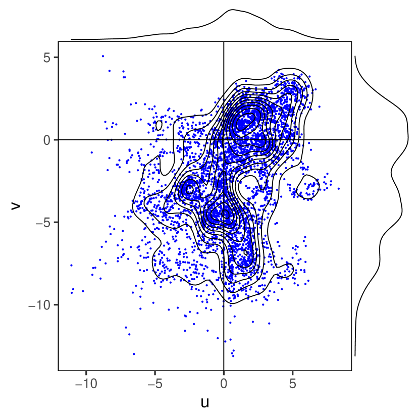
(a) $(u,v)$ representation

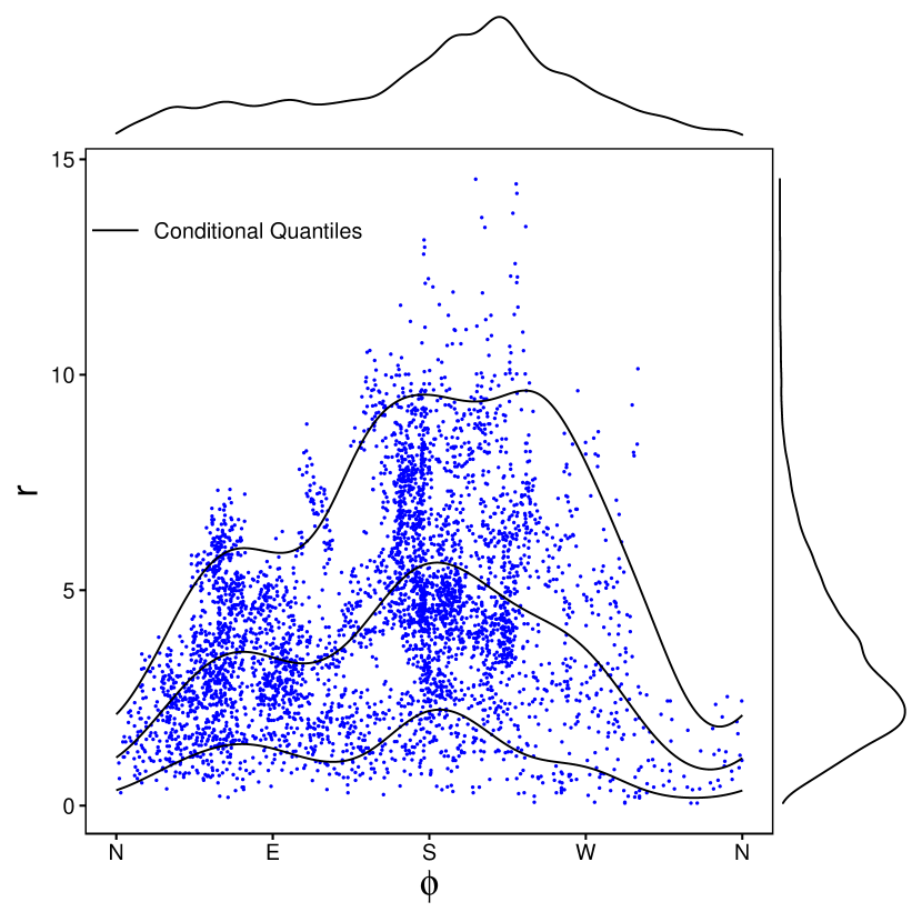
(b) $(r,\phi)$ representation

Figure 1: Representation of the wind vector in terms of Cartesian components with the corresponding marginal distributions and probability density contour curves (Left (a)) and polar coordinates with corresponding marginal distributions and $0.05$, $0.5$ and $0.95$ conditional quantile curves (Right (b)).

Under polar coordinates different statistical methods have been employed to model wind vector variations. Most existing works only consider the wind speed component of the wind vector, where there is a need to preserve the non-negativity and skewness properties. For a comprehensive review of commonly used distributions for modeling wind speed we refer the reader to (Carta et al., 2009).

Wind direction has received less attention in the literature because of its circular nature (Breckling, 1989), however, it can be important in many applications (e.g. coastal wind direction (Irish et al., 2013), animal behavior (Moen, 1982), fire spread (Abatzoglou et al., 2020)). A commonly used distribution for modeling wind direction is the von Mises distribution, or mixtures of von Mises distributions (Mardia, 1975). Wind direction can also be included in the modeling of the wind speed as a regime switching guidance (Hering and Genton, 2010; Ailliot et al., 2015; Ding, 2020) in which case the regime-switching can be represented as an observed or latent variable requiring the presence of a prevalent wind direction and a clear boundary for when to switch to a new regime. To eliminate the regime identification Hering and Genton (2010) propose that wind direction is used as a covariate in the modeling of the mean of the wind speed’s distribution. Specifically, the authors assume that the hourly wind speed follow a truncated normal distribution $N^{+}(\mu,\sigma^{2})$ and use sine and cosine functions to incorporate wind direction in modeling the mean, $\mu$.

Wind speed and wind direction typically exhibit an interdependent behavior: Fig. 1(b) shows that the (estimated) conditional quantile curves are directional dependent. Therefore, jointly modeling the distribution of wind speed and wind direction is needed. Copula approach can also be used here with a consideration that wind direction is a circular variable (Farlie, 1960; Plackett, 1965; Johnson and Wehrly, 1978). Under copula modeling framework, the joint distribution of wind speed and wind direction is separated into the marginal distributions of wind speed and wind direction, and a copula function that encodes the dependence structure of wind speed and wind direction under uniform marginals. Due to the circular nature of wind direction, there are fewer copula families that can be applied, which can be limited in modeling the wide various dependence structures of wind speed and wind direction.

In this work, we take an alternative approach to jointly modeling wind speed and wind direction by decomposing their joint distribution into the product of the marginal distribution of wind direction and the conditional distribution of wind speed given wind direction, i.e. $[R,\Phi]=[\Phi]\cdot[R|\Phi]$ (e.g., Coles and Walshaw, 1994; Solari and Losada, 2016; Wu et al., 2022). These aforementioned works model the conditional distribution by binning the data by wind direction to estimate the parameters of the chosen wind speed distribution separately, then use a set number of pairs of Fourier series to model the dependence of the wind speed distribution parameters on wind direction. While proving a useful modeling framework, to the best of our knowledge, there is no systematic study on various modeling choices; furthermore, no comparison study has been done to compare with some alternative methods in terms of estimation performance. Motivated by our recent work (Wu et al., 2022), this study aims to fill the gap by investigating these aspects.

In particular, we present an estimation and inference procedure, originally proposed in (Wu et al., 2022), to achieve flexible modeling of wind speed and wind direction that preserves the intrinsic characteristics of the two variables, namely non-negativity and circularity. This is done by using a mixture of von Mises distributions to perform the marginal modeling of wind direction, and the Weibull distribution for the conditional modelling of wind speed, where the parameters of the Weibull distribution are modeled by means of periodic functions on wind directions, which are fitted by a two-stage estimation procedure, where their estimation uncertainties are quantified via a version of block bootstrap (Kunsch, 1989a; Politis and Romano, 1991).

A simulation study is conducted to assess the performance of estimating the conditional distribution of wind speed using the proposed method and to compare it to a version of non-parametric quantile regression (QR) (Koenker, 2005) where the quantile curves are represented by a periodic B-spline as function of wind direction. Our results suggest that the proposed method in general outperforms the non-parametric QR we used. We illustrate our proposed method in a climate application where changes in the present and future wind speed and wind direction distributions are estimated using the output of a regional climate model. An advantage of the proposed methodology is that it allows for the detection of changes in the distribution of wind speed with respect to some wind directions giving us additional understanding about the distribution of wind speed.

The paper is structured as follows: Section 2 describes the proposed model and methods for estimation and inference. A simulation study investigating finite sample properties is described and the results are reported in Section 3. The proposed method is applied to a regional climate model data in Section 4 to study potential change of wind vector distribution under a future climate scenario. The paper concludes with a discussion and outlines of some future extensions in Section 5.

2 Joint Modeling of Wind Speed and Wind Direction

In this section we first present the models for estimating the wind direction distribution $[\Phi]$ and the conditional distribution of wind speed $[R|\Phi=\phi]$, respectively, which together determine the joint distribution $[R,\Phi]$. The model fitting procedure for each component will then be described with more emphasize on the estimation of $[R|\Phi=\phi]$, the main contribution of this work. We make use of a block bootstrap procedure, which is capable to preserve some aspect of the temporal dependence structure without explicitly modeling it, to quantify the estimation uncertainty. The non-parametric periodic spline QR, the benchmark method for estimating $[R|\Phi=\phi]$ in this study, will also be introduced.

2.1 Models

The joint distribution of wind speed and wind direction, $[R,\Phi]$, is decomposed into a product of the marginal distribution of the conditioning variable and the corresponding conditional distribution, i.e.

$$\left[R,\Phi\right]=\left[\Phi\right]\left[R|\Phi\right],$$ (1)

where $[\Phi]$ denotes the distribution of wind direction and $[R|\Phi]$ denotes the conditional distribution of wind speed given wind direction.

Such a decomposition allows to estimate the joint distribution using the “divide and conquer” strategy, where each one-dimensional estimation problem in the right-hand side can be modeled separately and flexibly via mixture modeling (Titterington et al., 1985; Lindsay, 1995b; McLachlan et al., 2019) and distributional regression (Fahrmeir et al., 2021) while avoiding the direct modeling of the potentially complex bivariate distribution in one step. This conditional decomposition approach is illustrated in Fig. 2, where flexible (yet relatively simple) models for $[\Phi]$ (second column) and $[R|\Phi]$ (third column) can produce quite complicated models for $[R,\Phi]$ and hence $[U,V]$ (fourth column).

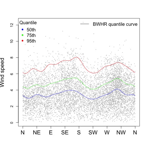
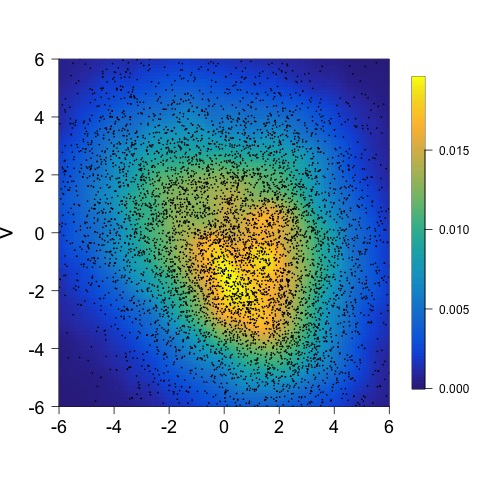
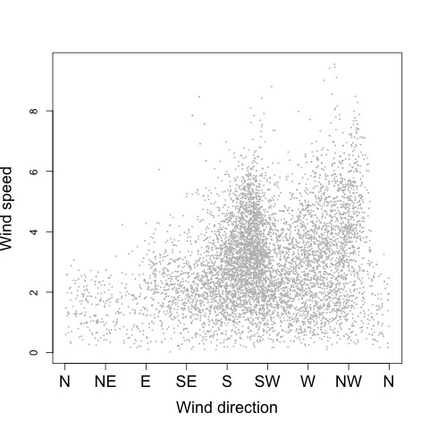
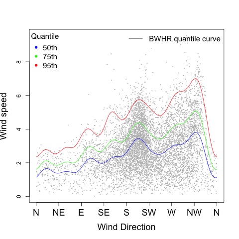
Figure 2: The wind data (first column) and the estimates of $[\Phi]$ (second column), $[R|\Phi=\phi]$ (third column), and the implied estimates of $[U,V]$ (fourth column) from a Texas great plain model grid cell (TX_GP, (top)), a North Dakota great plain grid cell (ND_GP, (middle)), and a North Carolina mountain grid cell (NC_mtn, (bottom)). More information regarding these data can be found in Section 4. To estimate the density of $[U,V]$ we simulated a large data set of wind directions from the $[\Phi]$ distribution and for each wind direction we simulated wind speeds from the $[R|\Phi=\phi]$ distribution. We transformed this data to the $(u,v)$ components and a two-dimensional kernel density estimation is applied to the simulated data.

We note that the decomposition can be done in the other way, where the conditioning variable is wind speed, i.e. in terms of $[R]$ and $[\Phi|R]$. However, it is arguably more natural to consider the conditional distribution of wind speed given wind direction than the conditional distribution of wind direction given wind speed. Furthermore, it is our view that it is easier to perform a distributional regression with a typical scalar response than a circular response. Finally, it is worth pointing out that the conditional distribution of wind direction given wind speed can be obtained by applying Bayes’ theorem, i.e., $[\Phi|R]=\frac{[\Phi][R|\Phi]}{[R]}$.

To model wind direction distribution $[\Phi]$, a mixture of $N_{\Phi}$ von Mises distributions (Mardia, 1972; Banerjee et al., 2005) is used. The von Mises distribution is a distribution commonly used for modeling circular data and has the following probability density function (pdf):

$$f_{vM}(\phi|\mu,\kappa)=\frac{1}{2\pi I_{0}(\kappa)}\exp\left[\kappa\cos(\phi-\mu)\right],$$ (2)

where $\mu\in[0,2\pi)$ and $\kappa\geq 0$ are the parameters of the distribution representing the directional mean and concentration of the distribution, respectively, and $I_{0}(\kappa)$ is the modified Bessel function of the first kind and order zero (Hill, 1977). However, the von Mises distribution is unimodal and therefore, may not produce a satisfactory fitting for wind direction data that is multimodal such as shown in the middle column of Fig. 2. Hence, our choice of using a finite mixture of von Mises distribution. Here, the density of the wind direction is modeled as follows:

$$f_{\Phi}(\phi|\mathbf{\mu,}\mathbf{\kappa},\mathbf{\omega})=\sum_{j=1}^{N_{\Phi}}\omega_{j}f_{vM}(\phi;\mu_{j},\kappa_{j}),$$ (3)

where $\omega_{j}$, $j=1,\ldots,N_{\Phi}$, are weights such that $\sum_{j=1}^{N_{\Phi}}\omega_{j}=1$.

To model $[R|\Phi]$, the conditional distribution of wind speed given wind direction (directional wind speed distribution hereafter), a parametric conditional distribution is assumed while allowing the parameters of the distribution be smooth yet flexible periodic functions of the wind direction. To this end, a Weibull distribution (Brown and R.W. Katz, 1984; Monahan, 2014) is considered where the parameters are modeled via Fourier series. The resulting pdf is given as follows:

$$f_{R|\Phi}(r|\phi,\alpha,\beta) = \left(\frac{\alpha(\phi)}{\beta(\phi)}\right)\left(\frac{r}{\beta(\phi)}\right)^{\alpha(\phi)-1}\exp\left[\left(-\frac{r}{\beta(\phi)}\right)^{\alpha(\phi)}\right],$$ (4)

$$\alpha(\phi) = b_{\alpha,0}+\sum_{k=1}^{K_{\alpha}}\Big{[}a_{\alpha,k}\cos(k\phi)+b_{\alpha,k}\sin(k\phi)\Big{]},$$ (5)

$$\beta(\phi) = b_{\beta,0}+\sum_{k=1}^{K_{\beta}}\Big{[}a_{\beta,k}\cos(k\phi)+b_{\beta,k}\sin(k\phi)\Big{]}.$$ (6)

2.2 Estimation Procedure

The parameters pertaining to the von Mises mixture distribution, $\mu_{j},\,\kappa_{j},\,\omega_{j}$, $j=1\ldots N_{\Phi}$, are estimated using the Expectation Maximization (EM) algorithm (Dempster et al., 1977; Banerjee et al., 2005). The number of von Mises components ($N_{\Phi}$) can be determined using the Bayesian information criterion (BIC) (McLachlan and Peel (2000), Chapter 6). Estimating the directional wind speed distribution $[R|\Phi=\phi]$ involves a pair of harmonic regression where the number of the harmonic terms is needed to be determined. Ideally, one could perform a likelihood-based estimation by fitting the directional dependent Weibull distribution to wind speed and direction data $\{r_{i},\phi_{i}\}_{i=1}^{n}$ with given $K_{\alpha}$ and $K_{\beta}$. However, it is our experience that doing so tends to be numerically unstable (see supplementary materials Sec. SM 1) and may lead to spurious fitted curves. The approach we take is a two-step procedure where the data points $\{r_{i},\phi_{i}\}_{i=1}^{n}$ are divided into $N$ bins in the direction domain, a Weibull distribution is fitted to wind speeds within each bin via maximum likelihood (ML) method. In the second step a pair of harmonic regression are conducted (equations (5) and (6) in the previous section, respectively) where the ML estimates across all bins (i.e., $\{\hat{\alpha}_{j}\}_{j=1}^{N}$, $\{\hat{\beta}_{j}\}_{j=1}^{N}$) are treated as the “responses”, where $N$ is the number of direction bins in the first step. Additionally, the estimated standard errors $\{\hat{\text{se}}(\hat{\alpha}_{j})\}_{j=1}^{N}$ and $\{\hat{\text{se}}(\hat{\beta}_{j})\}_{j=1}^{N}$ are incorporated to enable a weighted version of harmonic regression to be performed to estimate the parameters in equations (5) and (6).

Our estimation procedure involves several “tunning” parameters, namely, $N$ (number of bins), $K_{\alpha}$ and $K_{\beta}$ (number of pairs of trigonometric functions). We make the following suggestions for determining these values:

• The first suggestion pertains to binning the wind direction data using equal width or equal frequency (i.e., each bin contains the same number of data points) bins. Note that equal frequency binning approach leads to unequal bin sizes due to variation of wind direction distribution, hence resulting in an “uneven” modeling of $\alpha(\phi)$ and $\beta(\phi)$ in that of very little variation in the directions with sparse data while potentially too much variation in the directions that the data are dense. Therefore, we recommend using equal width directional bins, which in general gives better overall estimation performance (see supplementary material Sec. SM 2).

• Next, regarding the choice of the number of bins, $N$. Our sensitivity analysis (see supplementary material Sec. SM 2) suggests that choosing $N=36$ bins is enough to get a good estimation of the directional wind speed distribution as long as the size of the data set is sufficiently large (e.g., $n>3000$); additionally, there is no clear need to let $N$ grow with $n$ where $n$ is “large” because the “support” of $\Phi$ is fixed regardless of the sample size.

• In determining the number of pairs of Fourier series , i.e., $K_{\alpha}$ and $K_{\beta}$, one must have that $N\geq 2K+2$ to avoid having more parameters than the sample size ($N$ in this case) when fitting the harmonic regression in Step 2. For a chosen value of $N$, $K_{\alpha}$ and $K_{\beta}$ can be determined using BIC. However, we find that this strategy often gives to a “saturated” model, i.e., $N\approx 2K+2$ which leads to overfitting. Therefore, we suggest to use $K_{\alpha}=K_{\beta}=8$. This choice is compared to the choice of BIC and resulted in a smaller integrated mean relative error (MIRE, see its definition in Section 3.3) as shown in the supplementary material (Sec. SM 3).

We name the estimation method for $[R|\Phi=\phi]$ the Binned Weibull Harmonic Regression, BWHR hereafter, and we summarize it in Algorithm 1 below.

Algorithm 1 Binned Weibull - Harmonic Regression

Input: $\{r_{i},\phi_{i}\}_{i=1}^{n}$
First step: bin the wind data to estimate the parameters of the Weibull distribution and to compute a summary statistics of wind direction (e.g. medians) as follows:

• Bin the data by dividing the wind direction into $N$ bins, i.e. choose equal sized bins such that each bin has on average sufficient number of data points (e.g., 200 points).

• In each bin, represent wind direction data by a summary statistic, $\{\tilde{\phi}_{i}\}_{j=1}^{N}$, and fit a two parameter Weibull distribution to the wind speed data. The parameters of each of the Weibull distributions are estimated using Maximum Likelihood Estimation (MLE) method to obtain the estimates $\{\hat{\alpha}_{j},\hat{\beta}_{j}\}_{j=1}^{N}$ and their corresponding standard errors $\{\hat{\text{se}}(\hat{\alpha}_{j}),\hat{\text{se}}(\hat{\beta}_{i})\}_{j=1}^{N}$.

Second step: estimate the directional dependent function of Weibull parameters, $\alpha(\phi)$ and $\beta(\phi)$, using harmonic regression via WLS as follows:

• Use the direction summary statistic and the MLEs of each of the Weibull distributions as data points, i.e. $\{\tilde{\phi}_{j},\hat{\alpha}_{j}\}_{j=1}^{N}$ and $\{\tilde{\phi}_{j},\hat{\beta}_{j}\}_{j=1}^{N}$ , to regress the MLEs on the direction using periodic functions (e.g. a fixed $K$ pairs of harmonic functions): $\hat{\alpha}(\phi)=b_{\alpha,0}+\sum_{k=1}^{K}\Big{[}a_{\alpha,k}\cos(k\tilde{\phi})+b_{\alpha,k}\sin(k\tilde{\phi})\Big{]}$, $\hat{\beta}(\phi)=b_{\beta,0}+\sum_{k=1}^{K}\Big{[}a_{\beta,k}\cos(k\tilde{\phi})+b_{\beta,k}\sin(k\tilde{\phi})\Big{]}$. The weights (of WLS) are the squares of the inverses of the standard errors (SE) of the MLEs such that MLEs with lower SE receive higher weights than those with higher SE.

Output: $\alpha(\phi)$ and $\beta(\phi)$

Simulation-based approach can be used to obtain the implied joint distribution of $\widehat{[R,\Phi]}$ based on $[\hat{{\Phi}}]$ and $\widehat{[R|\Phi]}$. Specifically, one can simulate a large number of random variates, $\{\phi_{\text{sim},i}\}_{i=1}^{\ell}$ from $\hat{[\Phi]}$, and for each random variate $\phi_{\text{sim},i}$, simulate a paired random variate $r_{\text{sim},i}$, from $\widehat{[R|\Phi=\phi_{\text{sim},i}]}$. Transforming the simulated data $(\phi_{\text{sim},i},r_{\text{sim},i})_{i=1}^{m}$ using the transformation formulas presented in Section 1 we can approximate the distribution of $\widehat{[U,V]}$ up to a Monte Carlo sampling error, which is negligible with a large $\ell$.

2.3 Periodic Quantile Regression

Quantile regression (QR) is a general method for estimating conditional quantiles of the response variable $Y$. Rather than modeling the conditional mean of the response, i.e. $E[Y]$, as a function of the covariates $x$’s as commonly done in regression analysis, QR models the conditional quantile, i.e. $Q_{Y}(\tau|X)=\inf\{y:F(y|X)\geq\tau\}$, for quantile level $\tau\in(0,1)$ (Koenker and Bassett Jr, 1978). One can approximate the underlying conditional distribution $[Y|X]$ by estimating a set of conditional quantile levels (i.e. $Q_{Y}(\tau_{k}|X=x),\tau_{k}\in[0,1],k=1,\ldots,K,x\in\mathbb{R}$) (Mosteller and Tukey, 1977).

In this study, we model the $\tau$-quantile of the directional wind speed distribution ($[R|\Phi]$) using QR with periodic B-splines. The estimator of $Q_{R|\Phi}(\tau|\phi)$ takes the following form:

$$\hat{Q}_{R|\Phi}(\tau|\phi)=B(\phi)^{T}\hat{\beta}(\tau).$$ (7)

The vector $B(\phi)$ is a periodic B-spline with degree of freedom $df$. The periodic B-spline is used to preserve the circular property of the directional wind speed distribution while providing modeling flexibility in terms of quantile functions. We select the degree of freedom ($df=18$) by conducting a sensitivity study (supplementary material Sec. SM 4) and conclude that this choice leads to a reasonable compromise regarding bias and variance trade-off. The coefficient vector $\beta(\tau)$ is estimated as follows:

$$\hat{\beta}(\tau)=\arg\min_{\beta}\sum_{i=1}^{n}\rho_{\tau}(r_{i}-B(\phi_{i})^{T}\beta(\tau)),$$ (8)

where $\rho_{\tau}(y)=y(\tau-\mathbbm{1}_{(y<0)})$ is the quantile loss function. We call this periodic B-spline quantile regression model and its estimation procedure BPQR hereafter.

2.4 Estimation Uncertainty

To quantify the uncertainty associated with the parameter estimation we use a version of block bootstrap (Kunsch, 1989b) for both BWHR and BPQR. The block bootstrap is used in order to preserve the interannual temporal dependence presented in the climate application. Specifically, we draw 500 block bootstrap samples, where a block represents one year (Lahiri, 2003). In particular, since our data $\{r_{i},\phi_{i}\}_{i=1}^{n}$ represent wind speed and wind direction measured during one season we can arrange them into blocks, where each block represents a year. The $100\times(1-\alpha)\%$ bootstrap percentile interval is constructed using the $\frac{\alpha}{2}$ upper and lower percentiles. Fig. 3 shows these intervals for Texas Great Plain (TX_GP), North Dakota Great Plain (ND_GP) and North Carolina mountains (NC_mtn) location along with the computed $95\%$ quantile curve and empirical quantile estimates.

Figure 3: Top row: $95\%$ bootstrapped percentile confidence intervals of the $95\%$ quantile curve (black curve) using BWHR (red ) and BPQR (blue). The solid dots represent the (binned) empirical $95\%$ quantile estimates. Bottom row: Estimated wind direction distribution at three different locations.

3 Simulation Study

The purposes of this simulation study are fourfold: (i). to demonstrate how we implement the BWHR method, (ii). to assess the estimation performance of wind direction distribution, $[\Phi]$, by a von Mises mixture distribution, (iii). to compare the BWHR method to the BPQR in terms of $[R|\Phi=\phi]$, and (iv). to investigate the performance of the BWHR method in estimating the changes in the joint distribution of wind speed and direction.

3.1 Design

In this simulation study we mimic the joint distribution of wind speed and direction at three different locations presented in Section 4. Specifically, at each location the true data generating mechanism is estimated using the output from a regional climate model (see Section  4 for more details) by the followings:

1. Fit a bivariate Normal mixture distribution to $\{(u_{i},v_{i})\}_{i=1}^{n}$ of the model output. We purposely specify the data generating mechanism under the Cartesian coordinates to assess the flexibility of our conditional approach specified under the polar coordinates. The bivariate normal mixture fitting is done using the mclust() function from the mclust package (Scrucca et al., 2016) in R (R Core Team, 2021).

2. Transform the fitted bivariate normal mixture distribution to $[R,\Phi]$ distribution and compute the distribution of wind direction $[\Phi]$ and the conditional distribution $[R|\Phi]$.

For each location we generate 500 replicates, each having a sample size of 7360 wind speed and wind direction data points, corresponding to 3-hourly wind data of one season (assuming 92 days per season) over the course of 10 years. To evaluate the performance in estimating changes in the directional wind speed distribution, we apply the above steps to the model output for both historical and future scenario (see Section 4 for further details) to compute their differences. BWHR and PBQR are fitted to these simulated data and the estimated quantiles are subtracted to assess the estimation performance (see Section 3.3).

3.2 Illustration of BWHR

We use a simulated data series (see Fig. 4) to illustrate the BWHR and PBQR as described in Section 2. To estimate wind direction we use the movMF() function from the movMF (Hornik and Grün, 2014) package in R. The number of components of the von Mises mixture distribution is determined using BIC.

For the BWHR method we choose the number of bins to be $N=36$, so that there are, on average, about 200 data points across these bins, and we set $K_{\alpha}=K_{\beta}=8$. These choices were made following the suggestions from Section 2.2. A sensitivity analysis is included in the supplementary materials (Sec. SM 2 and SM 3). After determining $N$, $K_{\alpha}$, and $K_{\beta}$, Algorithm 1 can be applied to estimate $\alpha(\phi)$ and $\beta(\phi)$. The estimation performance of $[R|\Phi=\phi]$ is evaluated by examining a few selected quantile curves ($.5,.75$ and $.95$, see Fig.  4 for an example).

Figure 4: An illustration of applying the von Mises mixture distribution along with the BWHR and BPQR methods to a simulated data set. (Left) Wind direction distribution is estimated using a 4 component von Mises mixture distribution. (Right) We bin wind direction into $N=36$ equally spaced bins and we use $K_{\alpha}=K_{\beta}=8$ pairs of Fourier series to obtain the BWHR quantiles (solid lines); the BPQR (dashed lines) are computed using 18 degrees of freedom.

In implementing the BPQR method, we model each selected quantile of the directional wind speed distribution separately where a periodic B-spline is used to represent the directional quantile curve. We use the quantreg (Koenker, 2019) and pbs (Wang, 2013) packages in R (R Core Team, 2021) to carry out the estimation. In generating the periodic B-spline we need to determine the degrees of freedom ($df$). Based on a sensitivity analysis we choose $df=18$ to balance bias and variance.

3.3 Estimator Performance

It is important to incorporate wind direction distribution when quantifying the estimation performance. Therefore, we define the mean integrated relative error (MIRE) with respect to wind direction density, $f(\phi)$, specifically,

$$\mathrm{MIRE}=\int_{0}^{2\pi}\left\lvert\frac{\hat{g}(\phi)-g(\phi)}{g(\phi)}\right\rvert f(\phi)d\phi\,,$$ (9)

where $g(\phi)$ is the estimand (the quantity of interest) as a function of direction (e.g., directional $\tau$ - quantile of wind speed ($q_{\tau}(\phi)$), wind direction probability density function ($f(\phi)$), or quantile difference ($q_{\tau,\text{diff}}(\phi)$)). This metric is computed by discretizing the wind direction domain using a set of evenly spaced grid points $\{0<\phi_{1}<\phi_{2}<\ldots<\phi_{m}<2\pi\}$ with a sufficiently large $m$ (we use $m=629$ here) and using the following formula:

$$\mathrm{MIRE}\approx\frac{\sum_{i=1}^{m}f(\phi_{i})\left\lvert\frac{\hat{g}(\phi_{i})-g(\phi_{i})}{g(\phi_{i})}\right\rvert}{\sum_{i=1}^{m}f(\phi_{i})}.$$ (10)

We summarize the results of the simulation study in Table  1(c) - Table 1(c). In general, the wind direction distribution estimation performs reasonably well by using a mixture of von Mises distributions. At NC_mtn location, however, we note that the mixture of von Mises distributions is not able to capture well the distribution of wind direction, compared to the other locations, likely due to the fact that this is a mountainous region with a more complex wind direction distribution that is not well modeled by a von Mises mixture distribution. In the case of estimating the directional wind speed distribution, the BWHR method outperforms BPQR method at all three locations. Finally, when estimating changes in the directional wind speed distribution we conclude that the BWHR method is at least as good as BPQR in estimating changes in the directional wind speed distribution.

We close this section by exploring the conditions under one approach, BWHR method or the BPQR, works better than the other. As noted above, overall, the Weibull distributional regression is more accurate in estimating the directional wind speed distribution in terms of the MIRE. However, in the case of wind directions that have significantly lower occurrence probabilities (compared to other directions) BPQR performs slightly better. Moreover, representing the directional wind speed distribution using the BWHR allows for a data generating mechanism and, thus, we can use a simulation-based approach to examine the joint distribution of $[R,\Phi]$ (hence $[U,V]$ ) and their changes. We see this property as an advantage of BWHR over BPQR since QR method by itself does not completely determine the conditional distribution and hence the joint distribution.

Table 1: Boxplots of MIRE values of wind direction(top section), BWHR method, BPQR method (middle section), quantile differences (bottom section). The tables contain the MIRE values averaged over the 500 replicates along with the standard deviation values of MIRE of wind direction(top section), BWHR method, BPQR method (middle section), quantile differences(bottom section).

(a) Wind direction

TX_GP ND_GP NC_mtn (m/s) MvM MvM MvM MIREf(ϕ) 0.045 (0.008) 0.027 ( 0.008) 0.166 (0.019)

(b) Directional wind speed

	TX_GP		ND_GP		NC_mtn
(m/s)	PBQR	BWHR	PBQR	BWHR	PBQR	BWHR
MIRE${}_{q_{\tau=0.95}}$	0.022 (0.004)	0.017 (0.003)	0.028 (0.005)	0.021 (0.004)	0.093 (0.009)	0.074 (0.010)
MIRE${}_{q_{\tau=0.75}}$	0.017 (0.003)	0.014 (0.003)	0.024 (0.004)	0.020 (0.003)	0.093 (0.009)	0.070 (0.009)
MIRE${}_{q_{\tau=0.50}}$	0.020 (0.003)	0.019 (0.003)	0.029 (0.005)	0.023 (0.004)	0.088 (0.010)	0.075 (0.011)

(c) Directional quantile differences

	TX_GP		ND_GP		NC_mtn
(m/s)	PBQR	BWHR	PBQR	BWHR	PBQR	BWHR
MIRE${}_{q_{\tau=0.95}}$	0.258 (0.413)	0.215 (0.220)	0.467 (0.267)	0.371 (0.223)	0.426 (0.336)	0.401 (0.330)
MIRE${}_{q_{\tau=0.75}}$	0.166 (0.272 )	0.142 (0.163)	0.260 (0.139)	0.238 (0.146)	0.273 (0.214)	0.239 (0.197)
MIRE${}_{q_{\tau=0.50}}$	0.140 (0.267)	0.119 (0.148)	0.211 (0.143)	0.194 (0.114)	0.179 (0.136)	0.180 (0.131)

4 Application

The aim of this application is to estimate how the joint distribution of wind speed and direction may change from present to a possible future climate condition. According to the 2021 climate change report published by the Intergovernmental Panel on Climate Change (IPCC) (IPCC, 2021), research on the possible impact of climate change on wind patterns is warranted as it is a resource for clean energy. However, compared to temperature and precipitation, it is still uncertain how wind speed and direction distribution might change under future climate scenarios. For example, S.C.Pryor et al. (2009) found that observational data exhibit a decreasing trend in the annual mean wind speeds while reanalysis data show an increasing trend in the annual mean wind speeds. Furthermore, Wohland et al. (2019) show that reanalysis data from different Climate models show inconsistent trends in wind speed distribution. We aim to supplement these findings by examining any changes in the distribution of wind speed with respect to wind direction using our method BWHR.

4.1 Data Analysis

In this study we use 3-hourly output from 12km Weather Research and Forecasting (WRF) (Skamarock et al., 2008) regional climate simulations driven by the Community Climate System Model 4 (CCSM4) (Gent et al., 2011) under 10-year historical (1995-2004) and a future time-period (2085-2094) under a representative concentration pathway (RCP) 8.5 during the summer season (June, July, August) and winter season (December, January, February). More details on these simulations can be found in (Wang and Kotamarthi, 2015; Zobel et al., 2018a, b). To provide some spatial diversity of wind speed and wind direction distributions we use the output from three locations: Texas Great Plain (TX_GP), North Dakota Great Plain (ND_GP) and North Carolina mountains (NC_mtn) (see Fig.  5). Rose diagrams at these locations for summer and winter seasons are shown in Fig. 5. The distributions of wind speed and wind direction at these locations are depicted in the top row of Fig. 8 - 9, and Fig. 6, respectively. The wind direction distributions were chosen to feature different scenarios, in particular, ranging from a distribution concentrated around one direction to a distribution that is “evenly” distributed along all directions.

Figure 5: (Left) studied locations: Texas Great Plain (TX_GP), North Dakota Great Plain (ND_GP), North Carolina mountain (NC_mtn). We use the “+” symbol to denote the center of these grid cells. The map is colored by the ratio change in 10-year mean 95th-percentile of wind speed distribution projected by WRF driven by Community Climate System Model 4 (CCSM4), see data description in Section  4. (Right): Windrose diagrams for TX_GP (left column), ND_GP (middle column), and NC_mtn (right column) for summer (top row) and winter (bottom row).

4.2 Change in the Wind Direction Distribution

To investigate the changes in the wind direction we fit a von Mises mixture distribution to wind direction data at each location, where the number of components was chosen using the BIC. To quantify for the estimation uncertainty in wind direction we use the block boostrap procedure explained in Section 2. Fig. 6 illustrates that the estimated wind direction distribution at TX_GP remains relatively stable throughout both winter and summer seasons, showing minimal or negligible changes. Conversely, at ND_GP, there are indications of variations in wind direction, particularly towards northerly and southerly directions during the summer season. Similarly, at NC_mtn, changes in wind direction are observed specifically concerning westerly direction.

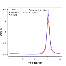
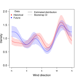
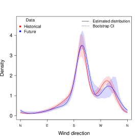
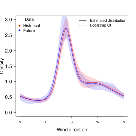
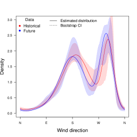
Figure 6: Bootstrap confidence intervals of historical (red color) and future (blue color) wind direction distributions during summer (top) and winter (bottom) seasons. Each column represents a different location.

4.3 Change in the Directional Wind Speed Distribution

To study the change in the directional wind speed distribution, we apply the BWHR method to $\{r_{i},\phi_{i}\}_{i=1}^{n}$ following the procedure described in Section 2. Fig. 7 presents the estimates of the $50\%$, $75\%$ and $95\%$ quantile curves at each of the locations.

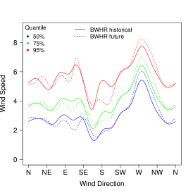
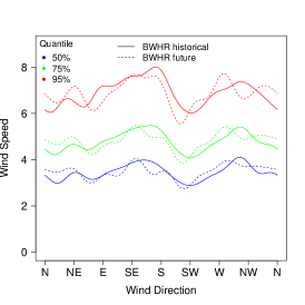
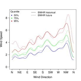
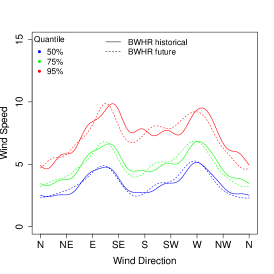
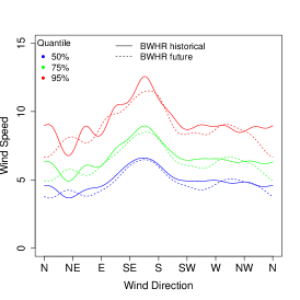
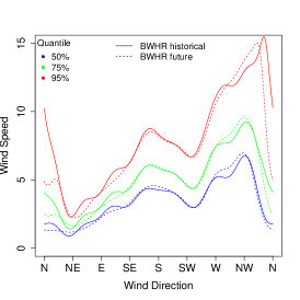
Figure 7: $50\%$ (blue), $75\%$ (green) and $95\%$ (red) conditional quantiles curves computed using the BWHR method of historical (solid lines) and future (dashed lines) summer (top row) and winter (bottom row) directional wind speed data. Each column represents a different location.

In order to assess any potential changes between the future and present directional wind speed distributions, we calculate the differences between the estimated future and present directional quantiles. To evaluate the added insights provided by our method in comparison to changes in wind speed distribution, we also calculate the estimated differences for the respective wind speed quantiles averaged across directions. We present the differences in the $95\%$ and $50\%$ of directional quantiles and wind speed quantiles along with their $95\%$ bootstrap confidence interval in Fig. 8 and Fig. 9. For the TX_GP location, our method reveals potentially greater changes in the $95\%$ directional quantile, particularly towards the South wind direction during summer and the Southeast wind direction during winter. These changes appear more pronounced than the $95\%$ quantile of the wind speed distribution. Similarly, in the case of ND_GP and NC_mtn, our method suggests considerably greater changes in the $95\%$ quantiles of the Northerly wind speeds than the $95\%$ quantile of wind speed.

We conclude this section by stating that the BWHR method allows for identifying changes in the wind speed distribution with respect to wind direction. If we had solely analyzed the differences in the quantiles of the wind speed distribution, we would have overlooked these differences.

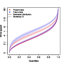
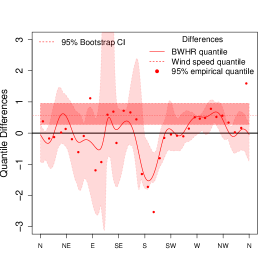
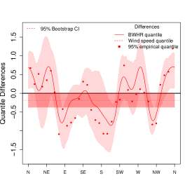
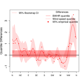
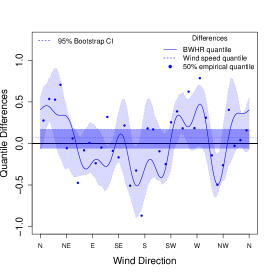
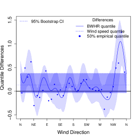
Figure 8: Summer wind data: Present (red) and future (blue) wind speed quantile curve (top row); Present and future quantile differences of the $95\%$ (middle row) and $50\%$ (bottom row) quantiles with the $95\%$ bootstrap confidence interval (shaded polygon); dotted horizontal lines in middle and bottom row, represent the quantile differences of present and future wind speed data and the darker shaded polygons represent the corresponding $95\%$ bootstrap confidence interval.

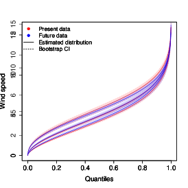
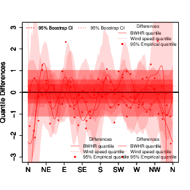
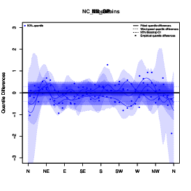
Figure 9: As in Fig. 8 but for winter season.

5 Summary and Discussion

In this work we develop a methodology for estimating the joint distribution of wind speed and wind direction through a conditional framework. The estimation is carried out by decomposing the bivariate distribution into the product of the marginal distribution of wind direction and the directional wind speed distribution, for which each component can be handle independently. For the marginal modeling of wind direction a von Mises mixture model is used, whereas for the modeling of the directional wind speed distribution we develop the BWHR method to estimate the directional dependent Weibull parameters, which can accommodate fairly flexible conditional distribution while maintaining the circular constraint.

A Monte Carlo simulation study is conducted to compare the model performance of the BWHR method to a periodic B-spline QR, BPQR. The results indicate that, for the three locations considered, BWHR performs better than BPQR in terms of the directional density weighted integrated mean relative error (MIRE). We illustrate this framework by applying the BWHR to estimate changes in the joint distribution of wind vector from present to future climate scenarios using the output from a regional climate model. Relative to the locations under consideration, our proposed methodology enables the detection of potential changes in wind speed given wind direction, in particular in the higher quantiles. Moreover, by taking into account the wind direction, our approach enables us to capture changes in wind speed that may have been overlooked if the wind direction was not taken into account. The proposed BWHR method is constructed using equally spaced bins. Nevertheless, one can also choose to bin wind direction that each bin includes the same amount of data points. We observe, however, that in this case, the model fails to appropriately capture the conditional quantile curves of the BWHR method when the wind direction data is sparse. This issue relates back to the conclusions made in Section 2.2 regarding the tuning parameter selection, that is, the bins are too large and estimating the wind speed distribution by Weibull distribution might be inappropriate. Furthermore, the BWHR method uses Fourier series to model the dependence structure between the Weibull parameters and wind direction. This dependence can also be modeled using periodic B-splines. In this case the degrees of freedom have to be determined. We find that this change gives a higher MIRE value compared to the method using Fourier series (see supplementary materials).

The method proposed in this study offers a procedure for modeling wind speed and direction measured at one location during one season. However, wind speed and wind direction exhibit a coherent spatial and temporal structure. Therefore, our intention is to extend this model to a spatio-temporal framework, considering the dependence on both space and time. To achieve this, we can incorporate spatio-temporal methods when modeling the parameters of the Weibull distribution, as suggested in previous studies (Rychlik, 2015; Mao and Rychlik, 2016). In the case of wind direction, it is necessary to account for both space and time in addition to allowing for spatial and temporal variation in the marginal distribution, This can be achieved by building upon the methodologies discussed in Wang et al. (2015); Mastrantonio et al. (2016), and Lagona (2022).

Supplementary information
Additional supplementary information can be found here.

References

- Abatzoglou et al. (2020) J. T. Abatzoglou, B. J. Hatchett, P. Fox-Hughes, A. Gershunov, and N. J. Nauslar. Global climatology of synoptically-forced downslope winds. International Journal of Climatology, 2020.
- Ailliot et al. (2015) P. Ailliot, J. Bessac, V. Monbet, and F. Pene. Non-homogeneous hidden Markov-switching models for wind time series. Journal of Statistical Planning and Inference, pages 75–88, 2015. doi: 10.1016/j.jspi.2014.12.005.
- Banerjee et al. (2005) A. Banerjee, I. Dhillon, J. Ghosh, and S. Sra. Clustering on the unit hypersphere using von Mises-Fisher distributions. Journal of Machine Learning Research, 6, 2005.
- Bessac et al. (2016) J. Bessac, P. Ailliot, J. Cattiaux, and V. Monbet. Comparison of hidden and observed regime-switching autoregressive models for ()-components of wind fields in the northeastern atlantic. Advances in Statistical Climatology, Meteorology and Oceanography, 2(1):1–16, 2016. doi: 10.5194/ascmo-2-1-2016. URL https://ascmo.copernicus.org/articles/2/1/2016/.
- Breckling (1989) J. Breckling. The analysis of directional time series: applications to wind speed and direction, volume 61. Springer Science & Business Media, 1989.
- Brown and R.W. Katz (1984) B. Brown and A. M. R.W. Katz. Time series models to simulate and forecast wind speed and wind power. Journal of Applied Meteorology and Climatology, 23, 1984.
- Carta et al. (2009) J. Carta, P. Ramírez, and S. Velázquez. A review of wind speed distributions used in wind energy analysis: Case studies in the Canary Islands. Renewable and Sustainable Energy Reviews, 13, 2009.
- Carta et al. (2008) J. A. Carta, P. Ramírez, and C. Bueno. A joint probability density function of wind speed and direction for wind energy analysis. Energy Conversion and Management, 49, 2008.
- Chen (2006) Q. Chen. Chapter 6: Wind in building environment design, Sustainable Urban Housing in China. Springer, 2006.
- Coles and Walshaw (1994) S. G. Coles and D. Walshaw. Directional modeling of extreme wind speeds. Journal of the Royal Statistical Society. Series C (Applied Statistics), 43, 1994.
- Dempster et al. (1977) A. Dempster, N. Laird, and D.B.Rubin. Maximum likelihood for incomplete data via the em algorithm. Journal of the Royal Statistical Society. Series B (Methodological), 39, 1977.
- Ding (2020) Y. Ding. Data Science for Wind Energy. Taylor & Francis Group, LLC, 2020.
- Fahrmeir et al. (2021) L. Fahrmeir, T. Kneib, S. Lang, and B. D. Marx. Distributional regression models. Springer Berlin Heidelberg, 2021.
- Farlie (1960) D. J. G. Farlie. The performance of some correlation coefficients for a general bivariate distribution. Biometrika, 47, 1960.
- Gent et al. (2011) R. Gent, G. Danabasoglu, L. Donner, M. Holland, E. Hunke, S. Jayne, D. Lawrence, R. Neale, P. Rasch, M. Vertenstein, and et.al. The community climate system model version 4. Journal of climate, 24(19): 4973-4991, 2011.
- Hering and Genton (2010) A. S. Hering and M. G. Genton. Powering up with space-time wind forecasting. Journal of the American Statistical Association, 105, 2010.
- Hill (1977) G. Hill. Algorithm 518: Incomplete bessel function . The von Misses distribution [S14]. ACM Transition of Mathematical Software, 3, 1977.
- Holmes and Bekele (2013) J. D. Holmes and S. Bekele. Wind Loading of Structures. Springer Science & Business Media, 2013.
- Hornik and Grün (2014) K. Hornik and B. Grün. movMF: An R package for fitting mixtures of von Mises-Fisher distributions. Journal of Statistical Software, 58(10):1–31, 2014. doi: 10.18637/jss.v058.i10.
- IPCC (2021) IPCC. Climate Change 2021: The physical science basis. Contribution of working group I to the Sixth Assessment Report of the Intergovernmental Panel on Climate Change. Cambridge University Press, Cambridge, United Kingdom and New York, NY, USA, In Press, 2021. doi: 10.1017/9781009157896.
- Irish et al. (2013) J. Irish, D. Resion, and J. Ratcliff. The influence of storm size on hurricane surge. Journal of Physical Oceanography, 38(9), 2013.
- Joe (1997) H. Joe. Multivariate models and dependence concepts. Chapman and Hall/CRC, 1997.
- Johnson and Wehrly (1978) R. A. Johnson and T. E. Wehrly. Some angular-linear distributions and related regression models. Journal of the American Statistical Association, 73, 1978.
- KNMI (2013) KNMI. Cesar database. Royal Netherlands Meteorological Institute (KNMI, the Netherlands), available at: http://www. cesar-database.nl/, 2013.
- Koenker (2005) R. Koenker. Quantile Regression. Cambridge University Press, 2005.
- Koenker (2019) R. Koenker. quantreg: Quantile regression, 2019. URL https://CRAN.R-project.org/package=quantreg. R package version 5.54.
- Koenker and Bassett Jr (1978) R. Koenker and G. Bassett Jr. Regression quantiles. Econometrica: journal of the Econometrics Society, pages 33-50, 1978.
- Kunsch (1989a) H. R. Kunsch. The jackknife and the bootstrap for general stationary observations. The Annals of Statistics, 17(3):1217–1241, 1989a.
- Kunsch (1989b) H. R. Kunsch. The jackknife and the bootstrap for general stationary observations. The annals of Statistics, pages 1217–1241, 1989b.
- Lagona (2022) F. Lagona. Spatial Autoregressive Models for Circular Data, pages 297–313. Springer Nature Singapore, Singapore, 2022. doi: 10.1007/978-981-19-1044-9_16. URL https://doi.org/10.1007/978-981-19-1044-9_16.
- Lahiri (2003) S. Lahiri. Resampling methods for dependent data. Springer - Verlag, 2003.
- Lindsay (1995a) B. G. Lindsay. Mixture models: theory, geometry, and applications. Ims, 1995a.
- Lindsay (1995b) B. G. Lindsay. Mixture models: theory, geometry and applications. NSF-CBMS Regional Conference Series in Probability and Statistics, 5:i–163, 1995b.
- Mao and Rychlik (2016) W. Mao and I. Rychlik. Estimation of weibull distribution for wind speeds along ship routes. Proceedings of the Institution of Mechanical Engineers, Part M: Journal of Engineering for the Maritime Environment, 231, 07 2016. doi: 10.1177/1475090216653495.
- Mardia (1972) K. V. Mardia. Statistics of directional data. Academic Press, 1972.
- Mardia (1975) K. V. Mardia. Statistics of directional data. Journal of the Royal Statistical Society. Series B (Methodological), 37, 1975.
- Mastrantonio et al. (2016) G. Mastrantonio, G. Jona Lasinio, and A. E. Gelfand. Spatio-temporal circular models with non-separable covariance structure. TEST, 25(3):331–350, 2016. doi: 10.1007/s11749-015-0458-y.
- McLachlan and Peel (2000) G. McLachlan and D. Peel. Finite mixture models. John Wiley and Sons, 2000.
- McLachlan et al. (2019) G. J. McLachlan, S. X. Lee, and S. I. Rathnayake. Finite mixture models. Annual review of statistics and its application, 6:355–378, 2019.
- McWilliams and Sprevak (1979) B. McWilliams and D. Sprevak. The probability distribution of wind velocity and direction. Wind Engineering, 3, No 4, 1979.
- Mendis et al. (2007) P. Mendis, T. Ngo, N. Haritos, and J. Samali, B.and Cheung. Wind loading on tall buildings. Electronic Journal of Structural Engineering, 7:41-54, 2007.
- Moen (1982) A. N. Moen. The biology and management of wild ruminants, Chapter Fourteen. CornerBrook Press, 1982.
- Monahan (2014) A. Monahan. Wind Speed Probability distribution, Encyclopedia of Natural Resources - Water and Air, volume 2. CRC Press, 2014.
- Mosteller and Tukey (1977) F. Mosteller and J. Tukey. Data analysis and regression: A Second Course in Statistics. Addison-Wesley Publishing Company, 1977.
- Nelsen (2006) R. B. Nelsen. An introduction to Copulas. Springer, 2006.
- Plackett (1965) R. L. Plackett. A class of bivariate distributions. Journal of the American Statistical Association, 60(310):516–522, 1965.
- Politis and Romano (1991) D. Politis and J. Romano. A circular block-resampling procedure for stationary data. Technical Report No. 370, tanford University, 1991.
- R Core Team (2021) R Core Team. R: A Language and environment for statistical computing. R Foundation for Statistical Computing, Vienna, Austria, 2021. URL https://www.R-project.org/.
- Reich and Fuentes (2007) B. Reich and M. Fuentes. A multivariate semiparametric Bayesian spatial modeling framework for hurricane surface wind fields. The Annals of Applied Statistics, 1, 2007.
- Rychlik (2015) I. Rychlik. Spatio-temporal model for wind speed variability. Annales de l’ISUP, 59(1-2):25–56, 2015. URL https://hal.archives-ouvertes.fr/ffhal-03604750f.
- S.C.Pryor et al. (2009) S.C.Pryor, R. Barthelmie, D. Young, E. Takle, R. Arritt, D.Flory, W. G. Jr., A. Nunes, and J.Roads. Wind speed trends over the contiguous United States. Journal of Geophysical Research, 114, 2009.
- Scrucca et al. (2016) L. Scrucca, M. Fop, T. B. Murphy, and A. E. Raftery. mclust 5: clustering, classification and density estimation using Gaussian finite mixture models. The R Journal, 8(1):289–317, 2016. URL https://doi.org/10.32614/RJ-2016-021.
- Skamarock et al. (2008) W. C. Skamarock, J. B. Klemp, D. O. Dudhia, J.and Gill, D. Barker, and J. G. Duda, M. G. … Powers. A description of the advanced research wrf version 3. ncar tech. note ncar/tn-475+str, 2008.
- Smith (1971) O. Smith. An application of distributions derived from the bivariate normal density function. Bulletin of the American Meteorological Society, 52, No. 3, 1971.
- Solari and Losada (2016) S. Solari and M. A. Losada. Simulation of non-stationary wind speed and direction time series. Wind Energy and Industrial Aerodynamics, 149, 2016.
- Stanley et al. (2020) A. P. J. Stanley, J. King, and A. Ning. Wind farm layout optimization with loads considerations. Journal of Physics: Conference Series, 1452, 2020.
- Titterington et al. (1985) D. M. Titterington, S. Afm, A. F. Smith, U. Makov, et al. Statistical analysis of finite mixture distributions, volume 198. John Wiley & Sons Incorporated, 1985.
- Wang et al. (2015) F. Wang, A. E. Gelfand, and G. Jona-Lasinio. Joint spatio-temporal analysis of a linear and a directional variable: Space-time modeling of wave heights and wave directions in the adriatic sea. Statistica Sinica, 25(1):25–39, 2015. URL http://www.jstor.org/stable/24311002.
- Wang and Kotamarthi (2015) J. Wang and V. R. Kotamarthi. High-resolution dynamically downscaled projections of precipitation in the mid and late 21st century over North America. Earth’s Future, 3(7):268–288, 2015.
- Wang (2013) S. Wang. pbs: Periodic B splines, 2013. URL https://CRAN.R-project.org/package=pbs. R package version 1.1.
- Weber (1997) R. O. Weber. Estimators for the standard deviation of horizontal wind direction. Journal of Applied Meteorology and Climatology, 36, 1997.
- Westerling et al. (2004) A. L. Westerling, D. R. Cayan, T. J. Brown, B. L. Hall, and L. G. Riddle. Climate, Santa Ana winds and autumn wildfires in Southern California. Eos, Transactions American Geophysical Union, 85(31):289–296, 2004.
- Wohland et al. (2019) J. Wohland, N. Omrani, D. Witthaut, and N. Keenlyside. Inconsistent wind speed trends in current twentieth century reanalyses. Journal of Geophysical Research: Atmosphere, 124, 2019.
- Wu et al. (2022) Q. Wu, J. Bessac, W. Huang, J. Wang, and R. Kotamarthi. A conditional approach for joint estimation of wind speed and direction under future climates. Advances in Statistical Climatology, Meteorology and Oceanography, 2022.
- Zannetti (2013) P. Zannetti. Air pollution modeling: theories, computational methods and available software. Springer Science & Business Media., 2013.
- Zobel et al. (2018a) Z. Zobel, J. Wang, D. J. Wuebbles, and V. R. Kotamarthi. Analyses for high-resolution projections through the end of the 21st century for precipitation extremes over the United States. Earth’s Future, 6(10):1471–1490, 2018a.
- Zobel et al. (2018b) Z. Zobel, J. Wang, D. J. Wuebbles, and V. R. Kotamarthi. Evaluations of high-resolution dynamically downscaled ensembles over the contiguous United States. Climate Dynamics, 50(3):863–884, 2018b.