Cross-Sectional Dynamics Under Network Structure: Theory and Macroeconomic Applications

Abstract

Many environments in economics feature a cross-section of units linked by bilateral ties. I develop a framework for studying dynamics of cross-sectional variables that exploits this network structure. It is a vector autoregression in which innovations transmit cross-sectionally via bilateral links and which can accommodate rich patterns of how network effects of higher order accumulate over time. The model can be used to estimate dynamic network effects, with the network given or inferred from dynamic cross-correlations in the data. It also offers a dimensionality-reduction technique for modeling high-dimensional (cross-sectional) processes, owing to networks’ ability to summarize complex relations among variables (units) by relatively few non-zero bilateral links. In a first application, I estimate how sectoral productivity shocks transmit along supply chain links and affect dynamics of sectoral prices in the US economy. The analysis suggests that network positions can rationalize not only the strength of a sector’s impact on aggregates, but also its timing. In a second application, I model industrial production growth across 44 countries by assuming global business cycles are driven by bilateral links, which I estimate. This reduces out-of-sample mean squared errors by up to 23% relative to a principal components factor model.

JEL codes: C32, E32, E37.

Key words: Vector Autoregression, Spatial Autoregression, Dynamic Network Effects, High-Dimensional Time Series, Sparse Factors, Input-Output Economy, Price Dynamics, Global Business Cycles.

1 Introduction

Numerous economic environments feature a cross-section of units connected by a network of bilateral ties. For example, countries are connected via flows of trade and capital, industries are linked through supply chains, and individuals in a society form a network by virtue of being acquainted to one another. As demonstrated theoretically and documented empirically, networks can rationalize comovement in variables measured at the cross-sectional level; GDP across countries varies depending on demand and supply by trade partners, firms adjust their prices in response to price increases by suppliers, individuals receive information and form opinions by interacting with their social network.

What is less well understood, however, is how network-induced comovements play out over time. With regard to the timing of network effects, the literature considers two restrictive cases. The first assumes that innovations transmit via bilateral links contemporaneously (e.g. Acemoglu et al. (2012); Elliott et al. (2014)). This leads to a static framework and implies that connections of all order play out (simultaneously). For example, an individual talks to all their friends, who in turn talk to all their respective friends, etc., so that at each point in time everyone’s opinion incorporates those of all members of society and within the same period fully adjusts to any new information gathered by even its most distant member. This assumption is useful for steady state comparisons, i.e. for stduying long-term effects of permanent shocks. The second case posits that network effects materialize exactly one link per period (e.g. Long and Plosser (1983); Golub and Jackson (2010)). This assumption is tenable in theoretical contributions, but in empirical studies a period is defined by data and it remains an empirical question how far a shock travels through the network in one observational period.

I build an econometric framework to study the dynamics of cross-sectional variables when units are connected through a network. It is a vector autoregression (VAR), parameterized such that innovations transmit cross-sectionally only via bilateral links. Transmission is assumed to be uni-directional and links fixed over time. The framework can accommodate rich patterns on how innovations travel along bilateral links over time, and, consequently, how network connections of higher order accumulate as time progresses. The interdependence of observations $y_{it}$ and $y_{j,t-h}$ arises as the interplay of temporal distance between periods $t$ and $t-h$ and cross-sectional distance between units $i$ and $j$ encoded by the network. Correspondingly, stationarity can be characterized in terms of eigenvalues of the network adjacency matrix and roots of an AR process defined by the timing of innovation transmission along a single link. This timing is fundamentally related to the frequency of network interactions relative to the frequency of observation.

The Network-VAR (NVAR) is useful in two rather distinct lines of empirical work with cross-sectional time series. On the one hand, it can be used to estimate dynamic network effects, i.e. to quantify how innovations transmit along bilateral links over time and come to shape cross-sectional dynamics. Thereby, the network can be taken as given or inferred from dynamic cross-correlations in the data, possibly aided by shrinking towards observed links. With both the network and effect-timing estimated, the NVAR is also applicable as a dimensionality-reduction technique for modeling high-dimensional processes. It assumes that dynamics are generated by innovation transmission along a (small) set of bilateral links among variables. Given the network, inference on the timing of network effects boils down to a linear regression with covariates that summarize lagged observations using bilateral links. Joint inference is implemented easily by iteration on analytically available conditional estimators, with Bayesian as well as frequentist interpretations. I illustrate each of these two model uses with a respective application.

In the first application, I estimate how sectoral productivity shocks propagate through the supply chain network and shape the monthly dynamics of Producer Price Indices (PPI) in the US economy. I show that the NVAR approximates the process of sectoral prices in a Real Business Cycle (RBC) input-output economy with time lags between the production of goods and their subsequent use as intermediaries in producing other goods. In turn, I estimate the timing of input-output conversion and its frequency relative to the monthly frequency of price observations. This allows me to determine the contribution of lagged input-output conversion in driving aggregate price dynamics and the impact of sectoral positions in the supply chain network on the timing at which sectoral price movements affect aggregate prices.

Preliminary results suggest that network positions have implications not only for the strength of sectoral shocks’ effects on aggregates – as documented in existing literature – but also for its timing, with no clear relationship between the two. How quickly a shock in a sector affects aggregate PPI is determined by the sector’s importance as an immediate – as opposed to further upstream – supplier to relevant sectors in the economy. Owing to their position at the top of supply chains, the response to price increases in energy-related sectors is estimated as particularly slow to unravel.

In the second application, I model industrial production growth across 44 countries by estimating an underlying network as relevant for dynamics. This provides a novel perspective on global business cycles by assuming that the dynamic comovement in economic activity across countries is the result of innovation transmission along bilateral links. The NVAR yields a sparse, yet flexible way of approximating (cross-sectional) processes even in high dimensions. Sparsity is obtained because dynamics are driven by bilateral links and because variables (units) can be connected even in absence of a direct link between them. As a result, the dynamic comovement of the whole, potentially high-dimensional time series can be modeled with relatively few non-zero bilateral links. This is reminiscent of the assumption that longer-term dynamics are driven by a set of shorter-term dynamics, which is upheld by the general class of VARMA($p,q$) models. Flexibility is owed to the fact that the network is estimated and that the model can accommodate general patterns of how network effects of higher order accrue over time.

An equivalence result suggests that the NVAR is preferred to a factor model whenever cross-sectional dynamics are composed of many micro links rather than driven by a few influential units. This corresponds to the case of numerous sparse factors with differing sets of non-zero loadings across units, or, equivalently, a sparse, yet high-rank network adjacency matrix. In my application, the NVAR – with the network estimated by shrinking links to zero – leads to reductions in out-of-sample mean squared errors of up to 23% relative to a principal components factor model, in particular for horizons up to six months.

Related Literature

This paper adds to the growing literature on networks in econometrics. In particular, there is a large literature on spatial autoregressive models. It is mostly concerned with identifying network effects (and effects of other covariates) in a static framework of contemporaneous dependencies (e.g. Manski (1993); Lee (2007); Bramoullé et al. (2009)). In contrast, I analyze lagged network effects. Relative to other studies in this category (e.g. Knight et al. (2016); Yang and Lee (2019)), Zhu et al. (2017) cast them in an explicit time series model, generalizing the lag length and discussing stationarity and large $T$-inference. I show that dynamics in this model – as evidenced by Granger causality at different horizons $h$ – are driven by innovation transmission along network connections of different order. In turn, I further generalize this mapping between network connections and dynamics, I discuss inference on both the timing of innovation transmission as well as on the network itself, and I illustrate the model’s merits as a dimensionality-reduction technique.

At a fundamental level, my work relates to Diebold and Yilmaz (2009, 2014), who map variance decompositions of VARs into networks with the goal of understanding dynamic connectedness. In contrast, I map networks into VARs. In particular, I use a network to model the conditional mean function, restricting innovations to transmit via bilateral links. This leads to rich patterns of multi-step causality, connecting my work to Dufour and Renault (1998). Relative to other studies restricting time series models using networks (e.g. Pesaran et al. (2004); Barigozzi et al. (2022); Mehl et al. (2023); Caporin et al. (2023)), I focus on a simple case of one variable per cross-sectional unit and one type of connection among units and I entertain this assumption of innovation transmission along bilateral links. This leads to a clear relation between the model’s time series properties on the one hand and the network and timing of network effects on the other. It also generates intuitive, analytical expressions for the estimators and allows me to examine the relation to factor models. Approaches for achieving shock identification using networks are discussed in Hipp (2020) and Dahlhaus et al. (2021). Bykhovskaya (2021) builds a time series model for the evolution of the network itself.

With my first application, I address the macroeconomic literature on production networks. It mostly assumes contemporaneous input-output conversion to show that networks amplify idiosyncratic shocks and generate cross-sectional comovement at a given point in time (Horvath, 2000; Foerster et al., 2011; Acemoglu et al., 2012; Bouakez et al., 2014; Giovanni et al., 2018; Giroud and Mueller, 2019). This framework is silent on how networks drive aggregate and cross-sectional dynamics. Exceptions are Long and Plosser (1983) and Carvalho and Reischer (2021), who study a Real Business Cycle (RBC) economy with input-output conversion lagged by one period. The former show that lagged input-output conversion leads to endogenous business cycles, while the latter characterize aggregate persistence in this theoretical model and show that it matches well empirical measures of persistence. Building on their work, I allow for more general lags in input-output conversion, which leads to sectoral prices (and output) in the model following an NVAR. In turn, I estimate the extent to which input-output conversion is spread out over several periods and its frequency relative to the monthly frequency of price observations. This allows me to determine the contribution of lagged input-output conversion in driving dynamics of aggregate prices.

With the second application of the NVAR, this paper addresses the vast literature on dimensionality-reduction techniques for time series modeling. By reducing the number of parameters and using shrinkage priors (regularization), the proposed approach applies both of the two ways of addressing the large parameter problem in the Wold representation (see Geweke (1984)). Compared to reduced rank regression and factor models (Velu et al., 1986; Stock and Watson, 2002), it finds the linear combination that effectively summarizes the information in lagged values by relying on bilateral links among variables (cross-sectional units). As a result, it naturally incorporates sparse factors as locally important nodes in the network, and it can improve upon the poor forecasting performance of factor models in settings with a high dispersion in factor loadings across series (see e.g. Boivin and Ng (2006)), such in this paper’s application. Compared to shrinkage methods like Lasso (Tibshirani, 1996) or Ridge regression, it applies shrinkage to links – which in turn summarize the information in predictors – rather than to predictors themselves. This leads to additional parsimony as the same links are used to summarize information at all lags, though possibly using different orders of connection.

The remainder of this paper is structured as follows. The model and its properties are discussed in Section 2. Section 3 treats inference. In Section 4, I study how input-output connections shape the dynamics of sectoral prices in the US economy, taking the network as given. In Section 5, I illustrate the merits of the NVAR as a dimensionality-reduction technique for modeling high-dimensional processes, and I apply it for forecasting cross-country industrial production. Section 6 concludes.

2 Lagged Network Effects & Cross-Sectional Dynamics

After providing some basic background on networks in Section 2.1, I present the NVAR in Section 2.2, building on a simple example. I explicitly examine the relation between the frequencies of network interaction and observation, and I discuss stationarity and the relation to contemporaneous network interactions. Estimation is deferred to Section 3.

2.1 Bilateral Connections in Networks

A network is represented by an $n\times n$ adjacency matrix $A$ with elements $a_{ij}$. I consider a directed, weighted and possibly signed network, which means that $a_{ij}\in[-1,1]$ shows the sign and strength of the link from cross-sectional unit $i$ to unit $j$, with $a_{ij}\neq a_{ji}$ possibly. If $a_{ij}=0$, I say unit $i$ is not connected to unit $j$. Self-links $a_{ii}\neq 0$ are permitted. The set of bilateral links $\{a_{ij}\}_{i,j=1:n}$ give rise to a plethora of higher-order connections among units, referred to as walks.

Definition 1 (Walk).

A walk from $i$ to $j$ of length $K$ is the product of a sequence of $K$ links $a_{i_{k},i_{k+1}}$ between units $i_{1},i_{2},...,i_{K-1}$ such that $a_{i_{k},i_{k+1}}\neq 0$ for $k=1:K-2$, with $i_{1}=i$, $i_{K-1}=j$:

$$a_{i,i_{2},...,i_{K-2},j}\equiv\prod_{k=1}^{K-2}a_{i_{k},i_{k+1}}\;.$$

Put simply, a walk is the product of bilateral links $a_{ij}$ that lead from unit $i$ to unit $j$ over some intermediary units, all of which are sequentially connected. Just as element $(i,j)$ in the matrix $A$ shows the walk from $i$ to $j$ of length one (direct link), simple matrix algebra reveals that $(A^{K})_{ij}$ contains the sum of walks from $i$ to $j$ of length $K$. I refer to this quantity as the $K$th-order connection from $i$ to $j$.

Consider the following example:

$$A=\begin{bmatrix}0&0&.8\\ .7&0&.6\\ 0&.8&0\\ \end{bmatrix}\;,\;\;A^{2}=\begin{bmatrix}0&.64&0\\ 0&.48&.56\\ .56&0&.48\\ \end{bmatrix}\;,\;\;A^{3}=\begin{bmatrix}.448&0&.384\\ .336&.448&.288\\ 0&.384&.448\\ \end{bmatrix}\;.$$

Even though unit $3$ is not directly connected to unit $1$ ($a_{31}=0$), there exists a second-order connection via unit $2$ ($a_{32}a_{21}\neq 0$). For example, in a production network, unit $1$ could be a supplier to unit $2$, who in turn is a supplier to unit $3$.

2.2 Lagged Innovation Transmission via Bilateral Links

The core assumption that underlies the proposed NVAR is that innovations $u_{it}$ to a process $y_{it}$ transmit cross-sectionally only via bilateral links. I assume links to be fixed and this transmission to operate only in one direction through the network. Specifically, the direct link from $i$ to $j$, $a_{ij}$, is a vehicle for innovation transmission from $j$ to $i$. Innovations can be cross-sectionally correlated. To simplify the exposition, I assume $\mathbb{E}[y_{it}]=0\;\forall\;i,t$.

2.2.1 Simple Example: NVAR(1,1)

Let $y_{t}=(y_{1t},...,y_{nt})^{\prime}$ and $u_{t}=(u_{1t},...,u_{nt})^{\prime}$, and consider the following VAR(1):

$$y_{t}=\Phi y_{t-1}+u_{t}\;,\quad u_{t}\sim WN(0,\Sigma)\;,\quad\quad\text{with}\quad\Phi=\alpha A\;,\quad\alpha\in\mathbb{R}\;,$$ (1)

Taking $\Phi$ to be proportional to the adjacency matrix $A$ of a network that connects the cross-sectional units, one obtains a process that relates the dynamics of the cross-sectional time series $y_{t}$ to the bilateral links among cross-sectional units. Long and Plosser (1983) derive such a process for sectoral output and prices in an RBC production economy with a one period delay in converting inputs into output. Golub and Jackson (2010) posit it to study societal opinion formation through friendship ties.

Under this process, the one period-ahead expectation of $y_{it}$ is proportional to a weighted sum of one period-lagged values of $y_{jt}$ for all units $j$ to which $i$ is directly linked, with weights given by the strength of direct links $a_{ij}$: $\mathbb{E}_{t-1}[y_{it}]=\alpha\sum_{j=1}^{n}a_{ij}y_{j,t-1}$. In the example from Long and Plosser (1983), the price charged tomorrow by firms in sector $i$ is expected to be a weighted average of prices charged by their suppliers today. Dynamics of $y_{t}$, as summarized by Granger-causality at horizons $h=1,2,...$, are shaped by $h$th order connections encoded in $A$:

$$GC_{ij}^{h}\equiv\frac{\partial y_{i,t+h}}{\partial y_{jt}}=\frac{\partial y_{i,t+h}}{\partial u_{jt}}=[\alpha^{h}A^{h}]_{ij}\;.$$

As a result, given all other variables $y_{k}\;,k\neq j$, $y_{j}$ is useful in forecasting $y_{i}$ at horizon $h$ iff there is an $h$th order connection from $i$ to $j$. The strength of this relationship is determined by the strength of this connection, i.e. by the sum of all walks from $i$ to $j$ of length $h$. Note that $GC_{ij}^{h}$ is also referred to as the Generalized Impulse Response Function (GIRF). It is generalized because it is not concerned with identification, but the derivative is taken with respect to (potentially correlated) reduced form errors in $u_{t}$.

Fig. 1 provides an example. It depicts the Granger-causality pattern for the process in Eq. 1 and the network from Section 2.1. Each panel $(i,j)$ shows the network connection from $i$ to $j$ at different orders $h$, $(A^{h})_{i,j}$, in blue, the decaying series $\alpha^{h}$ for $\alpha=0.9$ in red, and their product, the GIRF, in purple. By definition, the contemporaneous responses to all but a series’ own innovation are zero. From horizon $h=1$ onwards, the GIRF for every pair $(i,j)$ is proportional to the network connections from $i$ to $j$ of relevant order.

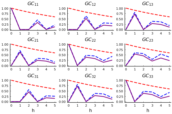
Figure 1: Example Generalized Impulse Responses: NVAR($1,1$)
Notes: Panel $(i,j)$ shows $(A^{h})_{ij}$ in blue, $\alpha^{h}$ in red and $GC^{h}_{ij}=(\alpha^{h}A^{h})_{ij}$ in purple.

Two points are worth highlighting. First, the relation between the shocked and responding unit in the network shapes not only the strength of the impulse-response, but also its timing. For example, while unit 2 is directly linked to unit 1 and therefore experiences the latter’s innovation with a lag of one period, unit 3 only has an indirect, second-order connection to unit 1 and is therefore impacted by its innovation only after two periods. Second, lagged network interactions can be a source of persistence, at the individual and aggregate level. Even without self-links – $a_{ii}=0$ – and autocorrelation in disturbances $u_{it}$, $y_{it}$ still persistently reacts to changes in $\{u_{jt}\}_{j\neq i}$ and $u_{it}$ because of lagged spillover and spillback effects. For example, unit 3 is linked to 2, which itself is linked to unit 3. Therefore, after an initial adjustment to its own disturbance, unit 3 experiences further rounds of adjustments because its initial response led to a response of unit 2. This is behind the endogenous business cycles in Long and Plosser (1983).

These results relate to the discussion in Dufour and Renault (1998), who point out that Granger-causality can take the form of chains. Specifically, even if a series $x_{t}$ does not Granger-cause a series $y_{t}$ at horizon 1, under the presence of a third series $z_{t}$, $x_{t}$ might Granger-cause $y_{t}$ at higher horizons as the causality could run from $x_{t}$ to $z_{t}$ to $y_{t}$. They examine conditions under which noncausality at a given horizon implies noncausality at higher horizons. If innovations transmit only via bilateral links, these generally non-trivial conditions boil down to the existence of network connections of relevant order between the concerned variables (units under cross-sectional time series).

While useful for theoretical work such as Long and Plosser (1983) and Golub and Jackson (2010), the process in Eq. 1 is of limited use empirically as it entertains a very restrictive mapping between network connections and observed dynamics in $y_{t}$. First, it presumes innovations travel through the network at the speed of one link per period, i.e. that the frequencies of network interactions and observation are equal. For instance, this implies that firms in sector $i$ do not adjust their price in response to price increases by suppliers situated two positions upstream of $i$ (suppliers of suppliers) earlier than with a lag of two periods. Second, it assumes complete transmission at a single lag. For example, after a price increase by a supplier-sector $j$, firms in sector $i$ fully adjust their own price after one period. Subsequent adjustments occur only to the extent that $j$ is also a supplier to other suppliers of $i$, whose adjustments to $j$ induce further adjustments of $i$. In the following, I extend the simple process above along both of these dimensions.

2.2.2 General Model: NVAR($p,q$)

Let the cross-sectional time series $\tilde{y}_{\tau}$ evolve according to

$$\tilde{y}_{\tau}=\alpha_{1}A\tilde{y}_{\tau-1}+...+\alpha_{p}A\tilde{y}_{\tau-p}+\tilde{u}_{\tau}\;,\quad\tilde{u}_{\tau}\sim WN(0,\Sigma)\;,$$ (2)

with $\alpha=(\alpha_{1},...,\alpha_{p})^{\prime}\in\mathbb{R}^{p}$. This is a particular version of the network-autoregressive process in Zhu et al. (2017). I dub this process NVAR($p,1$). Compared to Eq. 1, setting $p>1$ allows connections of order lower than $h$ to affect dynamics at horizon $h$.

Proposition 1 (Granger-Causality in NVAR($p,1$)).

Let $\tilde{y}_{\tau}$ evolve as in Eq. 2. Assuming $\alpha_{l}\neq 0\;\forall\;l$, $\tilde{y}_{j}$ Granger-causes $\tilde{y}_{i}$ at horizon $h$ iff there exists a connection from $i$ to $j$ of at least one order $k\in\{\underline{k},\underline{k}+1,...,h\}$, where $\underline{k}=ceil(h/p)$.

The proof in Appendix A establishes that the GIRF is of the form

$$\frac{\partial\tilde{y}_{i,\tau+h}}{\partial\tilde{u}_{j,\tau}}=c^{h}_{\underline{k}}(\alpha)\left[{A^{\underline{k}}}\right]_{ij}+...+c^{h}_{h}(\alpha)\left[{A^{h}}\right]_{ij}\;.$$ (3)

The coefficients $\{c^{h}_{k}(\alpha)\}_{k=\underline{k}:h}$ are polynomials of $\{\alpha_{l}\}_{l=1:p}$. They show the importance of different connection-orders for the impulse response at a given horizon $h$. Eq. 2 specifies that $\tilde{y}_{\tau}$ is shaped by lagged network interactions, whereby innovation transmission along a bilateral link takes $p$ periods to fully materialize. As elaborated on below, $\sum_{l=1}^{p}\alpha_{l}$ can be thought of as the overall strength of innovation transmission, while the individual elements in $\alpha$ show the time profile of this transmission. Note that it is assumed to be the same for all unit pairs $(i,j)$.

The process $\tilde{y}_{\tau}$ evolves at frequency $\tau$, which I shall call the network interaction frequency. It might not coincide with the frequency of observation. In particular, if data is observed at a lower frequency than network interactions occur – as is likely the case for macroeconomic series –, then dynamics at horizon $h$ can be driven by connections of order higher than $h$, as several rounds of transmission can happen in one period of observation. In addition, this leads to network-induced cross-sectional correlation in observed innovations even in absence of correlation in $\tilde{u}_{\tau}$. In the following, I formalize this idea, first for stock, then for flow variables. Let the observed data be $\{y_{t}\}_{t=1:T}$ and assume $\tilde{u}_{\tau}\sim N(0,\Sigma)$.

Time-Aggregation of Lagged Transmission Patterns

If $y_{t}$ is a stock variable, we can write $\{y_{t}\}_{t=1:T}=\{\tilde{y}_{tq}\}_{t=1:T}$ for some $q\in\mathbb{Q}_{++}$, i.e. we observe a snapshot of $\tilde{y}_{\tau}$ every $q$ periods. The dynamics of $y_{t}$ are represented by the state space system

$$\tilde{y}_{\tau} =\alpha_{1}A\tilde{y}_{\tau-1}+...+\alpha_{p}A\tilde{y}_{\tau-p}+\tilde{u}_{\tau}\;,\quad\tau=1:T_{\tau}\;,$$ (4)

$$y_{\tau/q} =\tilde{y}_{\tau}\quad\text{if}\;\tau/q\in\mathbb{N}\;.$$

I dub this process NVAR($p,q$) (for stock variables).

If $q^{-1}\in\mathbb{N}$, observational frequency either coincides with network interaction frequency ($q=1$) or is an integer-multiple thereof, which means that all $\tilde{y}_{\tau}$ are observed. Under Normality of $\tilde{u}_{\tau}$, dynamics of $y_{t}$ are represented by an NVAR($p/q,1$), with $p^{*}=p/q\in\mathbb{N}$:

$$y_{t}=\gamma_{1}Ay_{t-1}+...+\gamma_{p^{*}}Ay_{t-p^{*}}+u_{t}\;,\quad\gamma_{l}=\begin{cases}\alpha_{lq}\;\quad&\text{if $l$ is multiple of $q^{-1}$}\\ 0\;\quad&\text{otherwise}\end{cases}\;,\quad u_{t}\sim\tilde{u}_{\tau}\;,$$

For example, if network interactions occur at quarterly frequency, but observations are monthly, we have $q=1/3$, and the observed monthly series depends on its value three months ago, six months ago, etc., up to $3p$ months ago.

If $q\in\mathbb{N}\backslash\{1\}$, network interaction frequency is an integer-multiple of observational frequency such that we observe $\tilde{y}_{\tau}$ every $q$ periods. If $\tilde{y}_{\tau}$ is stationary, dynamics of $y_{t}$ can be approximated arbitrarily well by the following restricted VARMA process:

$$y_{t}\approx\sum_{l=1}^{p^{*}}\Phi_{l}y_{t-l}+u_{t}\;,\quad u_{t}=\sum_{l=0}^{p^{*}-1}\Theta_{l}\eta_{t-l}\;,\quad\Phi_{l}=\sum_{g=1}^{q^{*}}\gamma_{lg}A^{g}\;,$$ (5)

for $p^{*}$ large and $q^{*}=p^{*}q$. The coefficients $\gamma_{lg}$ are polynomials of $\{\alpha_{l}\}_{l=1:p}$ (or zero), and $\eta_{t}=(\tilde{u}_{\tau}^{\prime},...,\tilde{u}_{\tau-q+1}^{\prime})^{\prime}$ stacks all high-frequency innovations in-between the periods of observation $t-1$ and $t$. The $n\times nq$ matrices $\{\Theta_{l}\}_{l=0}^{p^{*}-1}$ are made up of $n \times n$ blocks, all of which are polynomials in $A$ of the form of $\Phi_{l}$. Section A.2 illustrates for the case of $p=3$ and $q=2$. For other cases with $q\in\mathbb{Q}_{++}$, the same result obtains as under $q\in\mathbb{N}\backslash\{1\}$.

The time-aggregation of lagged transmission patterns has interesting implications for the mapping from network connectedness to dynamics. Consider $q\in\mathbb{N}$. For $h=1,2,...$,

$$\frac{\partial y_{t+h}}{\partial y_{t}}=\frac{\partial\tilde{y}_{(t+h)q}}{\partial\tilde{u}_{tq}}=\frac{\partial\tilde{y}_{\tau+hq}}{\partial\tilde{u}_{\tau}}$$

is composed of network-connections of order $k\in\{ceil(hq/p),...,hq\}$. Because $\tilde{y}_{\tau}$ is observed every $q$ periods, up to $q$ rounds of transmission can occur in one period of observation, and connections of order up to $hq$ can matter at horizon $h$. Regarding the innovations to the observed process, $\eta_{t}=(\tilde{u}_{tq}^{\prime},...,\tilde{u}_{tq-q+1}^{\prime})^{\prime}$, we obtain that $\partial y_{t}/\partial\eta_{t}$ can be composed of connections of order $k\leq q-1$, depending on which of the high-frequency innovations $\tilde{u}_{tq},...,\tilde{u}_{tq-q+1}$ is behind the change in $\eta_{t}$. As a result, even if $\tilde{u}_{\tau}$ is not cross-sectionally correlated, there can be cross-sectional correlation in observed innovations $u_{t}$ if network interactions materialize at a higher frequency than data is observed.

If $y_{t}$ is a flow variable, we can write $y_{t}=\tilde{y}_{\tau}+...+\tilde{y}_{\tau-q+1}$ for $\tau=tq$ provided that $q\in\mathbb{N}$, i.e. the network interaction frequency either coincides with the observational frequency ($q=1$) or is an integer-multiple thereof. Dynamics of $y_{t}$ are are represented by the state space system

$$\tilde{y}_{\tau} =\alpha_{1}A\tilde{y}_{\tau-1}+...+\alpha_{p}A\tilde{y}_{\tau-p}+\tilde{u}_{\tau}\;,\quad\tau=1:T_{\tau}\;,$$ (6)

$$y_{\tau/q} =\tilde{y}_{\tau}+...+\tilde{y}_{\tau-q+1}\quad\text{if}\;\tau/q\in\mathbb{N}\;.$$

This is the NVAR($p,q$) for flow variables. Analogous conclusions about the dynamics of $y_{t}$ can be drawn as in the case of stock variables. For $q\notin\mathbb{N}$, no state space representation can be found for $y_{t}$ without assumptions that allow us to convert a flow variable from lower to higher frequency.

Contemporaneous Innovation Transmission Via Bilateral Links

The NVAR abstracts from contemporaneous network interactions, which feature prominently in the econometric literature on Spatial Autoregressive (SAR) models and the macroeconomic literature on production networks. In that case, the implicit assumption is that connections of all order materialize in any given period of observation:

$$x=Ax+\varepsilon=(I-A)^{-1}\varepsilon=(A+A^{2}+A^{3}+...)\varepsilon\;.$$

Contemporaneous interactions rationalize the cross-sectional comovement among $\{x_{i}\}_{i=1}^{n}$ as the network-induced amplification of cross-sectionally uncorrelated, idiosyncratic shocks $\{\varepsilon_{i}\}_{i=1}^{n}$. Ultimately, contemporaneous interactions concern shock identification, which is not the focus of this paper. Instead, the interest lies in how networks shape innovation transmission over time, regardless of the origin of these innovations.

Contemporaneous links are useful for quantifying overall connectedness via networks, but they are silent on how networks drive dynamics. Nevertheless, models with contemporaneous and lagged network interactions are related. By Proposition 8 in Section A.4, the (contemporaneous) response of $x_{i}$ to a (transitory or persistent) innovation to $x_{j}$ under contemporaneous interactions is equal to the long-run response of $y_{it}$ to a persistent innovation to $y_{jt}$ under lagged interactions in a corresponding NVAR($p,1$). Specifically, for

$$y_{t}=\alpha_{1}Ay_{t-1}+...+\alpha_{p}Ay_{t-p}+u_{t}\quad\quad\text{and}\quad\quad x=aAx+\varepsilon\;,\;\;a=\sum_{l=1}^{p}\alpha_{l}\;,$$

we have

$$lim_{h\rightarrow\infty}\left[{\frac{\partial y_{t+h}}{\partial u_{t}}+\frac{\partial y_{t+h}}{\partial u_{t+1}}+...+\frac{\partial y_{t+h}}{\partial u_{t+h}}}\right]=\frac{\partial x}{\partial\varepsilon}=(I-aA)^{-1}\;,$$

provided $y_{t}$ is stationary. Both responses are given by element $(i,j)$ of the Leontief inverse $(I-aA)^{-1}$, which is a sufficient statistic for the long-term (or overall, static) cross-sectional comovement of interest. The difference between the two specifications is that, by taking a stance on the time profile of network interactions, $y_{t}$ contains information on how any such long-term effect materializes over time. In contrast, the timing of interactions is irrelevant if the interest lies only in steady state comparisons rather than transition dynamics. As shown in Section A.4, the same result applies even if only a snapshot or an average of realizations from such an NVAR($p,1$) is observed every $q$ periods, $q\in\mathbb{N}\backslash\{1\}$.

Note that the timing of the long-term response to a permanent shock provides evidence on the timing of this impulse-response more generally, regardless of the nature of the shock. This is because for any VAR, the response to a permanent shock is equal to the cumulative response to a temporary shock (to the same variable). Therefore, the fraction of the long-term response which materialized until horizon $h$ is equal to the area under the IRF to a temporary shock until horizon $h$ as a fraction of the total area. As a result, a slow long-term response to a permanent shock implies a persistent response to a temporary shock.

3 Inference

The NVAR can be used to estimate dynamic peer effects or model high-dimensional (cross-sectional) processes more generally, say for forecasting purposes. In either case, one might have data on the network $A$ and be willing to condition on it, or one might prefer to infer it from the data. In Section 3.1, I discuss the estimation of the time profile of network effects $\alpha$, conditioning on $A$. In Section 3.2, I discuss joint inference on $(\alpha,A)$, with $A$ identified from dynamic cross-sectional correlations in the data, possibly aided by shrinking towards observed network links.

3.1 Timing of Network Effects

The first part of this section is devoted to the estimation of $\alpha$ in the NVAR($p,1$). The second part deals with the case when data is observed at a higher frequency than network interactions take place, i.e. stock variables in the NVAR($p,q$) with $q>1,q\in\mathbb{Q}$ and flow variables in the NVAR($p,q$) with $q>1,q\in\mathbb{N}$. Details are in Section B.1.

NVAR($p,1$)

The NVAR($p,1$) from Eq. 2,

$$y_{t}=\alpha_{1}Ay_{t-1}+...+\alpha_{p}Ay_{t-p}+u_{t}\;,\quad\alpha=(\alpha_{1},...,\alpha_{p})^{\prime}\in\mathbb{R}^{p}\;,$$

can be written as a linear regression:

$$y_{t}=X_{t}\alpha+u_{t}\;,\quad\text{or}\quad y_{it}=x_{it}^{\prime}\alpha+u_{it}\;,$$ (7)

where the $n\times p$ matrix $X_{t}$ summarizes the information in lags $1:p$ of $y_{t}$ using first-order network connections:

$$X_{t}=\begin{bmatrix}x_{1t}^{\prime}\\ ...\\ x_{nt}^{\prime}\end{bmatrix}=\big{[}Ay_{t-1},Ay_{t-2},...,Ay_{t-p}\big{]}\;.$$ (8)

Because the network $A$ is taken as given, the dependence of $X_{t}$ on it is suppressed.

Defining $\Sigma=\mathbb{V}[u_{t}]$, we obtain the following Least Squares (LS) estimator for $\alpha$:

$$\hat{\alpha}|\Sigma=\left[{\sum_{t=1}^{T}X_{t}^{\prime}\Sigma^{-1}X_{t}}\right]^{-1}\left[{\sum_{t=1}^{T}X_{t}^{\prime}\Sigma^{-1}y_{t}}\right]\;.$$ (9)

As usual, it is also the Maximum Likelihood (ML) estimator under Normality of $u_{t}$ and the posterior mean and mode under a Uniform prior for $\alpha|\Sigma$. Under $\Sigma=I$, it yields the Ordinary LS (OLS) estimator, which takes the form of a pooled OLS estimator:

$$\hat{\alpha}_{OLS}=\left[{\sum_{t=1}^{T}X_{t}^{\prime}X_{t}}\right]^{-1}\left[{\sum_{t=1}^{T}X_{t}^{\prime}y_{t}}\right]=\left[{\sum_{i=1}^{n}\sum_{t=1}^{T}x_{it}x_{it}^{\prime}}\right]^{-1}\left[{\sum_{i=1}^{n}\sum_{t=1}^{T}x_{it}y_{it}}\right]\;.$$

Section B.1 establishes consistency and asymptotic Normality of $\hat{\alpha}_{OLS}$ under large $T$, large $n$ and large $(n,T)$ asymptotics. The derivations under large $n$ assume that the observed network adjacency matrix $A_{n}$ converges to some limit $A$ so that, for example, $\frac{1}{n}\sum_{i=1}^{n}\left({A_{n,i\cdot}y_{t-l}}\right)^{\prime}u_{it}\overset{p}{\rightarrow}\mathbb{E}\left[{\left({A_{i\cdot}y_{t-l}}\right)^{\prime}u_{it}}\right]$.

NVAR($p,q$) with $q>1$

As discussed in Section 2.2.2, if $\tilde{y}_{\tau}$ follows an NVAR($p,1$) and a snapshot of $\tilde{y}_{\tau}$ is observed every $q$ periods, i.e. $\{y_{t}\}_{t=1}^{T}=\{\tilde{y}_{tq}\}_{t=1}^{T}$ for $q>1,q\in\mathbb{Q}$, the dynamics of $y_{t}$ are represented by the state space system from Eq. 4:

$$\tilde{y}_{\tau} =\alpha_{1}A\tilde{y}_{\tau-1}+...+\alpha_{p}A\tilde{y}_{\tau-p}+\tilde{u}_{\tau}\;,\quad\tau=1:T_{\tau}\;,$$

$$y_{\tau/q} =\tilde{y}_{\tau}\quad\text{if}\;\tau/q\in\mathbb{N}\;,$$

and similarly if $\tilde{y}_{\tau}$ and $y_{t}$ are flow variables and $\{y_{t}\}_{t=1}^{T}=\{\tilde{y}_{tq}+...+\tilde{y}_{(t-1)q+1}\}_{t=1}^{T}$ for $q>1,q\in\mathbb{N}$ is observed (see Eq. 6).

In principle, an estimator for $\alpha$ could be obtained by data augmentation. However, point identification is not guaranteed. For example, under $q=2$ and $p=1$, the observed process follows

$$y_{t}=\alpha_{1}^{2}A^{2}y_{t-1}+\eta_{t}\;,\quad\text{with}\;\;\eta_{t}=\tilde{u}_{2t}+\alpha_{1}A\tilde{u}_{2t-1}\;,$$

which suggests that $\alpha_{1}$ is identified only up to sign. The identification problem is akin to estimating an AR($p$) observed every $q$ periods, discussed in Palm and Nijman (1984), or estimating continuous time models using discrete time data (see e.g. Phillips (1973)). As in these cases, the mapping between the parameters $\alpha$ in the high-frequency process $\tilde{y}_{\tau}$ and the parameters in the observed process $y_{t}$ is not bijective.

As a remedy, Palm and Nijman (1984) suggest adding prior information. Recall that $\{\alpha_{l}\}_{l=1:p}$ is the GIRF for units $i$ and $j$ that only share a first-order connection (see Section 2.2.2). The following prior induces smoothness in this GIRF by shrinking $\{\alpha_{l}\}_{l=1:p}$ to a quadratic functional form:

$$\alpha_{l}\sim N\left({\mu_{l},\lambda_{\alpha}^{-1}}\right)\;,\quad\mu_{l}=w^{\alpha\prime}_{l}\beta_{\alpha}\;,\quad w^{\alpha}_{l}=(1,l,l^{2})^{\prime}\;.$$

This leads to the full-sample posterior

$$\alpha_{l}|\tilde{Y}_{1:T_{\tau}}\sim N\left({\bar{\alpha},\bar{V}_{\alpha}}\right)\;,\quad\bar{V}_{\alpha}=\left[{\sum_{\tau=1}^{T_{\tau}}\tilde{X}_{\tau}^{\prime}\tilde{\Sigma}^{-1}\tilde{X}_{\tau}+\lambda_{\alpha}I_{p}}\right]^{-1}\;,\quad\bar{\alpha}=\bar{V}_{\alpha}\left[{\sum_{\tau=1}^{T_{\tau}}\tilde{X}_{\tau}^{\prime}\tilde{\Sigma}^{-1}\tilde{y}_{\tau}+\lambda_{\alpha}I_{p}\mu}\right]\;,$$

where $\mu=W^{\alpha}\beta_{\alpha}$, $\tilde{\Sigma}=\mathbb{V}[\tilde{u}_{\tau}]$ and $\tilde{X}_{\tau}$ is the analogue of $X_{t}$ for $\tilde{y}_{\tau}$.

Conditioning on $\tilde{\Sigma}$, $\beta_{\alpha}$ and $\lambda_{\alpha}$, the posterior $p(\alpha|Y_{1:T})$ can be obtained by treating the unobserved data in $\tilde{Y}_{1:T_{\tau}}$ as parameters and finding first the joint posterior $p(\alpha,\tilde{Y}_{1:T_{\tau}}|Y_{1:T})$. This is implemented numerically using the Gibbs sampler of Carter and Kohn (1994), by iteratively drawing from $p(\tilde{Y}_{1:T_{\tau}}|\alpha,Y_{1:T})$ and $p(\alpha|\tilde{Y}_{1:T_{\tau}})$. As $\lambda_{\alpha}\rightarrow 0$, the resulting posterior mode of $\alpha$ converges to the ML estimator obtained using the Expectation-Maximization (EM) algorithm. Due to the identification problem, this mode may not be unique. For $\lambda_{\alpha}\rightarrow 0$, the suggested Bayesian approach traces out all the modes and shows the extent of the identification problem. For $\lambda_{\alpha}>0$, it remedies the identification problem as the posterior mean weighs these modes by shrinking $\{\alpha_{l}\}_{l=1:p}$ to the quadratic function $\{(1,l,l^{2})\beta_{\alpha}\}_{l=1:p}$.

Using a hierarchical Bayes approach, the exact function to which $\alpha$ is shrunk and the optimal amount of shrinkage can be inferred from the data by specifying uniform hyperpriors for $\beta_{\alpha}$ and $\lambda_{\alpha}$. As discussed in Giannone et al. (2015), under uniform hyperpriors, the shape of the posterior of hyperparameters coincides with that of the marginal likelihood, a measure of model fit and out-of-sample predictive ability. This leads to Normal and Gamma conditional posteriors:

$$\beta_{\alpha}|\alpha,\lambda_{\alpha} \sim N\left({\bar{\beta}_{\alpha},\bar{V}_{\beta_{\alpha}}}\right)\;,\quad\text{with}\quad\bar{V}_{\beta_{\alpha}}=\left[{\lambda_{\alpha}W^{\alpha\prime}W^{\alpha}}\right]^{-1}\;,\quad\bar{\beta}_{\alpha}=\bar{V}_{\beta_{\alpha}}\left[{\lambda_{\alpha}W^{\alpha\prime}\alpha}\right]\;,$$

$$\lambda_{\alpha}|\alpha,\beta_{\alpha} \sim G\left({\frac{p}{2}+1\;,\;\frac{1}{2}(\alpha-W^{\alpha}\beta_{\alpha})^{\prime}(\alpha-W^{\alpha}\beta_{\alpha})}\right)\;,$$

where $W^{\alpha}$ stacks $w^{\alpha}_{l}=(1,l,l^{2})^{\prime}$ along rows. The joint posterior $p(\alpha,\beta_{\alpha},\lambda_{\alpha},\tilde{Y}_{1:T_{\tau}}|Y_{1:T})$ is then obtained by augmenting the above Gibbs sampler with two additional iteration steps, drawing from $p(\beta_{\alpha}|\alpha,\lambda_{\alpha})$ and $p(\lambda_{\alpha}|\alpha,\beta_{\alpha})$. Fixing $\lambda_{\alpha}\rightarrow\infty$, we impose $\alpha_{l}=(1,l,l^{2})\beta_{\alpha}$, and the posterior mode of $\beta_{\alpha}$ converges to the ML estimator for $\beta_{\alpha}$ from the EM algorithm.

To estimate $\tilde{\Sigma}$, an additional step is added to the Gibbs sampler. Using a uniform prior, we get an Inverse-Wishart conditional posterior:

$$\Sigma|\alpha,\tilde{Y}_{1:T_{\tau}}\sim IW(\tilde{U}^{\prime}\tilde{U},T_{\tau})\;,$$

where the $T_{\tau}\times n$ matrix $\tilde{U}$ stacks $\tilde{u}_{\tau}=\tilde{y}_{\tau}-\tilde{X}_{\tau}\alpha$ along rows. Its mode is $\frac{1}{T_{\tau}}\sum_{\tau=1}^{T_{\tau}}\tilde{u}_{\tau}\tilde{u}_{\tau}^{\prime}$.

3.2 Joint Estimation: Network & Effect-Timing

No matter whether one is interested in estimating dynamic peer effects or approximating dynamics of cross-sectional processes, in many cases network data might be missing or it appears restrictive to condition on the available data. This section discusses joint estimation of $(\alpha,A)$. Again the first part deals with the estimation of an NVAR($p,1$), while the second part discusses the case of an NVAR($p,q$) with $q>1$.

NVAR($p,1$)

To facilitate the estimation of $A$, the NVAR($p,1$) from Eq. 2,

$$y_{t}=\alpha_{1}Ay_{t-1}+...+\alpha_{p}Ay_{t-p}+u_{t}\;,\quad\alpha=(\alpha_{1},...,\alpha_{p})^{\prime}\in\mathbb{R}^{p}\;,$$

can also be written as the linear regression

$$y_{t}=Az_{t}+u_{t}\;,\quad\text{or}\;\;Y=ZA^{\prime}+U\;,$$ (10)

whereby $z_{t}=\sum_{l=1}^{p}\alpha_{l}y_{t-l}=\big{[}y_{t-1},y_{t-2},...,y_{t-p}\big{]}\alpha$, and the $T\times n$ matrices $Y$, $Z$ and $U$ stack $y_{t}$, $z_{t}$ and $u_{t}$ along rows, respectively. To simplifty notation, I suppress the dependence of $z_{t}$ on $\alpha$ and that of $X_{t}$ on $A$.

To render $(\alpha,A)$ jointly identified, I normalize $||\alpha||_{1}=1$. Alternatively, one could fix one $\alpha_{l}$ to some value, with appropriate redefinitions of $\alpha$ as well as $y_{t}$, $z_{t}$ and $X_{t}$. As elaborated on below, the former normalization is easier to implement. The latter facilitates asymptotic analysis, but requires $\alpha_{l}\neq 0$ in the true data generating process.

Suppose data on a network $B$ with elements $b_{ij}$ is available. Under independent priors $a_{ij}\sim N(b_{ij},\lambda_{a}^{-1})$, we obtain a matrix-variate Normal conditional posterior for $A$:

$$A|Y,\alpha,\Sigma,B,\lambda_{a}\sim MN\left({\bar{A}^{\prime},\Sigma,\bar{U}_{A}}\right)\;,\quad\text{with}\;\;\bar{U}_{A}=\left[{Z^{\prime}Z+\lambda\Sigma}\right]^{-1}\;,\;\;\bar{A}=\bar{U}_{A}\left[{Z^{\prime}Y+\lambda B^{\prime}\Sigma}\right]\;.$$

Its mean and mode, $\bar{A}^{\prime}$, is equal to the conditional optimizer for $A$ under a LS objective function with a Ridge-penalty:

$$\bar{A}^{\prime}=\arg\underset{A}{min}\; \frac{1}{nT}\sum_{t=1}^{T}\left({y_{t}-Az_{t}}\right)^{\prime}\Sigma^{-1}\left({y_{t}-Az_{t}}\right)+\frac{1}{nT}\lambda_{a}\sum_{i,j=1}^{n}(a_{ij}-b_{ij})^{2}\;.$$ (11)

As $\lambda_{a}\rightarrow\infty$, the conditional posterior converges to a pointmass at $B$. As $\lambda_{a}\rightarrow 0$, $A$ is inferred from the data alone. No domain restrictions on $A$ are imposed because any parameter value $(\alpha,A)$ can be rescaled to yield $a_{ij}\in[-1,1]\;\forall\;i,j$, so that $A$ can be interpreted as a network. A Normal rather than Laplace prior (i.e. a Ridge rather than Lasso penalty) is chosen for analytical convenience.

Conditioning on $\lambda_{a},\lambda_{\alpha},\beta_{\alpha}$, the joint posterior $p(\alpha,A,\Sigma|Y)$ is again obtained by Gibbs sampling, iterating on the conditional posterior $p(A|Y,\alpha,\Sigma,B,\lambda_{a})$ from above as well as $p(\alpha|Y,A,\Sigma,\beta_{\alpha},\lambda_{\alpha})$ and $p(\Sigma|\alpha,A,Y)$ from Section 3.1. To impose the normalization $||\alpha||_{1}=1$, draws from $p(\alpha|Y,A,\Sigma,\beta_{\alpha},\lambda_{\alpha})$ are appropriately rescaled in every iteration. Setting $\lambda_{\alpha}\rightarrow 0$, the posterior mode is equal to the GLS estimator ($\hat{\alpha},\hat{A},\hat{\Sigma})$, obtained by iterating on $\hat{\Sigma}|(\alpha,\Sigma)=\frac{1}{T}\sum_{t=1}^{T}u_{t}(\alpha,A)u_{t}(\alpha,A)^{\prime}$ and the conditional optimizers $\hat{\alpha}|(A,\Sigma)$ and $\hat{A}|(\alpha,\Sigma)$ of the objective function in Eq. 11 above. Fixing in addition $\Sigma=I$, we obtain the OLS estimator $\hat{\theta}_{OLS}$ of $\theta=(\alpha,A)$, for which consistency and asymptotic Normality under $T\rightarrow\infty$ are established in Section B.2.

Analogously as done for $\lambda_{\alpha}$ and $\beta_{\alpha}$, under hierarchical modeling and a uniform or improper prior for $\lambda_{a}$, we obtain

$$\lambda_{a}|A,B \sim G\left({\frac{n^{2}}{2}+1\;,\;\frac{1}{2}\sum_{i,j=1}^{n}(a_{ij}-b_{ij})^{2}}\right)\;.$$

The joint posterior $p(\alpha,A,\Sigma,\lambda_{a},\lambda_{\alpha},\beta_{\alpha}|Y)$ is obtained by iterating on the six conditional posteriors. As $\lambda_{a}\rightarrow\infty$, we condition on the network $B$, just as done in Section 3.1 above.

The network $B$ can be constructed as a combination of multiple link-types. Collecting the latter in the vector $w^{b}_{ij}$, we can set $b_{ij}=w_{ij}^{b\prime}\beta_{b}$. To infer the network that best rationalizes the data, augment this specification with hyperpriors $\beta_{b}\sim N(0,\lambda_{b}^{-1}I)$ and $p(\lambda_{b})\propto c$. This results in conditional posteriors

$$\beta_{b}|A,\lambda_{a},\lambda_{b} \sim N\left({\bar{\beta}_{a},\bar{V}_{\beta_{b}}}\right)\;,\quad\text{with}\quad\bar{V}_{\beta_{b}}=\left[{\lambda_{a}W^{a\prime}W^{b}+\lambda_{b}I}\right]^{-1}\;,\quad\bar{\beta}_{a}=\bar{V}_{\beta_{b}}\left[{\lambda_{a}W^{a\prime}vec(A)}\right]\;,$$

$$\lambda_{b}|\beta_{b} \sim G\left({\frac{dim(\beta_{b})}{2}+1\;,\;\frac{1}{2}\beta_{b}^{\prime}\beta_{b}}\right)\;,$$

where $W^{b}$ is s.t. $W^{b}\beta_{b}=vec(B)$. As $\lambda_{b}\rightarrow\infty$, the conditional posterior of $\beta_{b}$ converges to a pointmass at zero and links $a_{ij}$ are shrunk to zero. As $\lambda_{b}\rightarrow 0$, the conditional posterior of $\beta_{b}$ is centered at the OLS estimator from a regression of $b_{ij}$ on $w_{ij}^{b}$.

NVAR(p,q) with $q>1$

As in the estimation of $\alpha|A$, under an NVAR($p,q$) with $q>1$, joint inference on $(\alpha,A)$ can be conducted relying on data augmentation. The joint posterior is obtained using the Gibbs sampler of Carter and Kohn (1994). As before, identification from data alone is not guaranteed, but the problem is ameliorated by shrinking $\alpha$ to a known functional form and $A$ to a known or sparsely parameterized network $B$. Note that the identification problem is irrelevant if only properties of the process at observational frequency are of interest.

4 Input-Output Links & Sectoral Price Dynamics

How do price innovations propagate across sectors in an economy? Given an observed price increase in, say, energy-related sectors, what is the expected path of aggregate prices? With sectors linked by an input-output network, the answers depend on the positions of the shocked (and responding) sector in the network as well as on the velocity at which a shock travels through the network.

The literature so far mostly assumed contemporaneous input-output conversion to show that the supply chain network amplifies idiosyncratic sectoral shocks – with stronger amplification for more central sectors – and that input-output linkages can rationalize the comovement of sectoral prices at a given point in time. Exceptions are Long and Plosser (1983) and Carvalho and Reischer (2021), who assume one-period-lagged input-output conversion. The former show that this leads to endogenous business cycles, while the latter characterize aggregate persistence in this theoretical model and show that it matches well empirical measures of persistence. In the following, I allow for more general lags in input-output conversion and estimate to what extent it can account for persistence in aggregate prices and, hence, whether input-output linkages can rationalize also the dynamic comovement of sectoral prices over time.

Consistent the literature, I consider the propagation of relative price changes induced by supply-side TFP shocks, as motivated by an input-output economy in the Real Business Cycle (RBC) tradition. Assuming that firms’ production in each sector requires the inputs produced in other sectors in the past $p$ periods, sectoral prices and output in this economy evolve at some model-frequency according to an NVAR($p,1$). The network $A$ is the input-output matrix, while $\{\alpha_{l}\}_{l=1:p}$ show how input-sourcing is spread out over the $p$ periods. By estimating $\alpha$ as well as the frequency of input-output conversion relative to my monthly frequency of observation, I determine the role of lagged input-output conversion in driving the observed dynamics of sectoral prices.

After theoretically motivating the analysis in Section 4.1, I discuss the data in Section 4.2 and the estimation procedure in Section 4.3. Results are presented in Section 4.4.

4.1 Theory

This section extends a benchmark input-output economy by introducing time lags in input-output conversion. The analysis is based on Carvalho and Tahbaz-Salehi (2019), who discuss a static economy. Details are provided in Section C.1.

Assume there are $n$ sectors, in each of which a representative firm produces a differentiated good $i$ by combining labor services $l_{it}$ and goods produced by other sectors $j$, $\{x_{ijt}\}_{j=1}^{n}$, using a Cobb-Douglas production function. Firms maximize profits, taking prices as given. The profits of firm $i$ in period $t$ are

$$\Pi_{it}=p_{it}y_{it}-w_{t}l_{it}-\sum_{j=1}^{n}p_{jt}x^{ij}_{t}\;,\quad\text{with}\;\;y_{it}=z_{it}l_{it}^{b_{i}}\prod_{j=1}^{n}x_{ijt}^{a_{ij}}\;,$$

where $b_{i}>0$, $a_{ij}\geq 0$ and $b_{i}+\sum_{j=1}^{n}a_{ij}=1$. $z_{it}$ denotes TFP in sector $i$ and $w_{t}$ the price of labor. $x_{ijt}$ is the amount of good $j$ used in the production at time $t$. As discussed below, it can differ from the amount of good $j$ purchased in period $t$, $x^{ij}_{t}$. $a_{ij}$ shows the importance of good $j$ in the production of good $i$. Under perfect competition and constant returns to scale (CRS) Cobb-Douglas production functions, prices are entirely determined by supply. Nevertheless, to show that the following results hold in general equilibrium and to obtain results for output dynamics, in Section C.1 I assume a representative household which supplies one unit of labor inelastically and exhibits log-preferences over the $n$ goods.

Different assumptions on the timing of input-output conversion lead to different dynamics of sectoral prices and output in this economy. Let $x^{ij}_{t,t-h}$ denote the use of good $j$ purchased at time $t-h$ in the production of good $i$ at time $t$. Most of the literature assumes that inputs are converted into outputs in the same period when they are produced and purchased, i.e. $x_{ijt}=x_{t,t}^{ij}=x^{ij}_{t}$. This leads to a static economy with contemporaneous network effects. Dropping time-subscripts, we obtain the following equation for sectoral prices $p=(p_{1},...,p_{n})^{\prime}$ as a function of sectoral productivities $z=(z_{1},...,z_{n})^{\prime}$ and input-output relations summarized by the input-output matrix $A$:

$$\tilde{p}=k^{p}+A\tilde{p}+\varepsilon\;,$$

where $\tilde{p}=ln(p/w)$, $\varepsilon=-ln(z)$ and $k^{p}$ is a vector of constants. This equation fully characterizes prices in this economy, whereby wages are taken as the numéraire.

To analyze dynamics under lagged input-output conversion, I assume perfect foresight. If, as in Long and Plosser (1983) and Carvalho and Reischer (2021), it takes one period to convert purchased inputs into output, then $x_{ijt}=x^{ij}_{t,t-1}=x^{ij}_{t-1}$ and sectoral prices approximately follow an NVAR(1,1):

$$\tilde{p}_{t}=k^{p1}_{t}+A\tilde{p}_{t-1}+\varepsilon_{t}\;,$$

where $k^{p1}_{t}=k^{p1}-(\iota-b)ln\left({G^{w}_{t}}\right)$. $k^{p1}$ is a vector of constants, $\iota$ is a vector of ones, $b=(b_{1},...,b_{n})^{\prime}$ contains sectoral labor shares and $G^{w}_{t}=w_{t}/w_{t-1}$ is wage growth in period $t$. This process only deviates from an NVAR($1,1$) to the extent that the numéraire $w_{t}$ changes in value. This result can trivially be extended to input-output conversion at single lags of arbitrary length; if it takes $p$ periods to convert inputs into output, $\tilde{p}_{t}$ approximately follows an NVAR($p,1$) with coefficients in front of all but the $p$th lag equal to zero.

Differences between the steady states in this economy and the above economy with contemporaneous interactions vanish as firms’ discount factor $\beta\longrightarrow 1$. However, while the latter is always in steady state, this economy is dynamic and after a disturbance to $\varepsilon_{t}$ only asymptotically converges to steady state. For empirical analyses one has to take a stance on what a period in this model signifies relative to an observational period in the data.

Dynamics are driven by several lags if firms in their production at time $t$ use inputs produced in several past periods. To model this case, I assume that $x_{ijt}$ aggregates quantities of input $j$ purchased at different periods in the past using a Constant Elasticity of Substitution (CES) aggregator. This shortcut stands for frictions like stochastic or time-varying input delivery time and storage capacity constraints. To keep the exposition tractable, let $x_{ijt}$ include amounts of good $j$ bought at $t-1$ and $t-2$, $x^{ij}_{t,t-1}$ and $x^{ij}_{t,t-2}$:

$$x_{ijt} =\left[{\eta_{1}(x^{ij}_{t,t-1})^{r}+\eta_{2}(x^{ij}_{t,t-2})^{r}}\right]^{1/r}\;,$$

with $\eta_{1},\eta_{2}\geq 0$, $\eta_{1}+\eta_{2}=1$ and $r>0$. An extension to general lengths $p$ is straightforward. The homogeneity of parameters $\eta_{1}, \eta_{2}$ implies that the time profile of input-sourcing is constant over time and across input-output pairs $(i,j)$.

In the Cobb-Douglas case $r\rightarrow 0$, sectoral prices approximately follow an NVAR(2,1):

$$\tilde{p}_{t}=k^{p2}_{t}+\eta_{1}A\tilde{p}_{t-1}+\eta_{2}A\tilde{p}_{t-2}+\varepsilon_{t}\;,$$

where $k^{p2}_{t}=k^{p2}-(\iota-b)\left[{\eta_{1}ln\left({G^{w}_{t}}\right)+\eta_{2}ln\left({G^{w}_{t}G^{w}_{t-1}}\right)}\right]$. Again, this relation is only approximate to the extent that the numéraire changes in value. Under a more general elasticity of substitution, excluding the case of perfect substitutability ($r=1$), a similar result is obtained by log-linearizing around the steady state. Let a hat denote percentage deviation from steady state. We obtain

$$\hat{\tilde{p}}_{t}=\hat{k}^{p3}_{t}+\chi_{1}\check{A}\hat{\tilde{p}}_{t-1}+\chi_{2}\check{A}\hat{\tilde{p}}_{t-2}+\hat{\varepsilon}_{t}\;,\quad\chi_{1},\chi_{2}\geq 0\;,\;\;\chi_{1}+\chi_{2}=1\;.$$

The elements of $\check{A}$ are scaled bilateral links $a_{ij}/(1+b_{i}(1-r))$, while $\hat{\varepsilon}_{t}$ contains scaled TFP deviations $\hat{\varepsilon}_{it}=-\hat{z}_{it}/\phi_{i}$, with $\phi_{i}=(1+b_{i}(1-r))/(2-r)$. These scalings vanish under perfect substitutability, $r\rightarrow 1$. The vector $\hat{k}^{p3}_{t}$ is composed of elements $\hat{k}^{p3}_{it}=(1-\phi_{i})/\phi_{i}\hat{y}_{it}+(1-b_{i}/\phi_{i})\left[{\chi_{1}\hat{G}^{w}_{t}+\chi_{2}(\hat{G}^{w}_{t}+\hat{G}^{w}_{t-1})}\right]$. Hence, for general elasticities of substitution $r$, the process of sectoral prices differs from an NVAR(2,1) not only to the extent that the numéraire changes, but also as sectoral output changes. The output-term vanishes as $r\rightarrow 1$.

To sum up, under general lags in input-output conversion, the log of sectoral prices, now denoted by $\tilde{y}_{\tau}$, evolves at some model-frequency approximately as an NVAR($p,1$):

$$\tilde{y}_{\tau}\approx\alpha_{1}A\tilde{y}_{\tau-1}+...+\alpha_{p}A\tilde{y}_{\tau-p}+\tilde{u}_{\tau}\;,$$

with $\alpha_{l}\geq 0\;\forall\;l$ and $\sum_{l=1}^{p}\alpha_{l}=1$, where $\tilde{u}_{\tau}$ is proportional to the vector of TFP shocks, and where $A$ contains input shares $a_{ij}$, with $\sum_{j}a_{ij}<1\;\forall\;i$. These restrictions render the process stationary.

Several assumptions are crucial for this result. First, perfect competition implies that prices equal marginal costs and prevents strategic price setting. Second, Cobb-Douglas production functions imply constant input shares regardless of prices and prevent upstream propagation of TFP shocks. This makes clear that the rows of $A$ contain the production recipes for firms in each sector, which firms adhere to in every period. Third, input-sourcing is constant over time and across input-output pairs $(i,j)$, which leads to a homogeneous $\alpha$.

4.2 Data

To construct $A$, I use annual data on input-output matrices provided by the Bureau of Economic Analysis (BEA). Due to availability of PPI data, I consider the level of 64 mostly three- and four-digit sectors rather than the finer level of around 400 six-digit commodities (NAICS classification). The analysis is restricted to non-farm and non-governmental sectors. I take the input-output matrix for 2010, roughly the midpoint of the sample of sectoral Producer Price Indices (PPI) (see below). Following Acemoglu et al. (2016), links $a_{ij}$ are calibrated as

$$a_{ij}=\frac{sales_{j\longrightarrow i}}{sales_{i}}\;,$$

where $sales_{j\longrightarrow i}$ is the total value of goods and services purchased by sector $i$ from sector $j$ as determined by the corresponding entry in the BEA’s “use” table. The value of $a_{ij}$ shows how many dollars worth of output of sector $j$ sector $i$ needs to purchase in order to produce one dollar’s worth of its own output. This calibration of $a_{ij}$ assumes that firms’ input shares reported for the course of a year are equal to the unobserved input shares at higher frequency intervals.

Monthly data for the corresponding sector-level PPIs is obtained from the Bureau of Labor Statistics (BLS). Data availability narrows the analysis to 51 sectors and the time frame January 2005 - August 2022. This includes the Great Recession as well as the COVID-19 recession. More details on the matching of PPI and input-output data are provided in Section C.2.

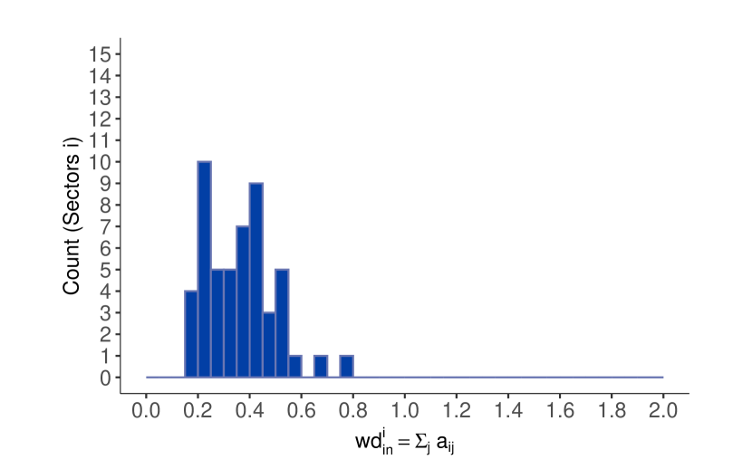
(a) Weighted In-Degrees

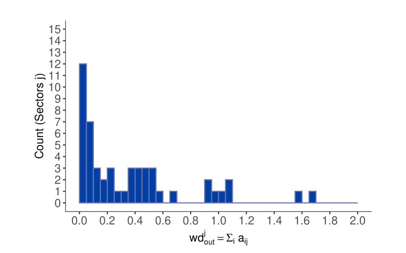
(b) Weighted Out-Degrees

Figure 2: Weighted In-Degrees & Out-Degrees
Notes: The left panel plots weighted in-degrees, equal to the column-wise sums of $A$, which show the differing reliance on intermediate inputs across sectors. The right panel plots weighted out-degrees, equal to the row-wise sums of $A$, which show the differing importance of a sector as a supplier to other sectors in the economy.

The majority of links in the network are weak. Even though the fraction of non-zero links is 73.55%, only 16.88% are above 0.01. Nevertheless, and as expected at this level of aggregation, this network density is much higher than the 3% reported for the finer level of 417 sectors in Carvalho (2014). As illustrated in the left panel of Fig. 2, weighted in-degrees, $wd^{in}_{i}\equiv\sum_{j}a_{ij}$, lie below 1 for all sectors, as posited by theory. The heterogeneity in this statistic across sectors shows that they rely to different extent on intermediary inputs in production. The right panel shows the weighted out-degrees, $wd^{out}_{j}\equiv\sum_{i}a_{ij}$, and illustrates that most sectors are specialized input-suppliers, while there are also a few general-purpose suppliers. The average distance in the network is 2.41. This means that each sector is on average 1.4 in-between suppliers away from other sectors. The longest distance, or diameter of the network, is 7, which means that it takes at most 6 in-between suppliers for a sector to reach another sector. Section C.2 contains more details on input-output data.

The left panel in Fig. 3 depicts the raw PPI series for a few sectors. It provides evidence of considerable heterogeneity in price dynamics across sectors, even disregarding the highly volatile energy-sectors. The right panel of Fig. 3 shows that an output-weighted average of sectoral PPIs included in the analysis replicates the actual aggregate PPI fairly well, despite the fact that some sectors are excluded due to data limitations. Aggregate PPI shows a clear upward trend, with a smaller spike around the Great Recession as well as a very pronounced spike in the aftermath of the COVID-19 recession. To render the PPI series stationary, I estimate and subtract a linear trend and a seasonality component for each sector $i$. In the theoretical model, any time trends in sectoral prices are due to idiosyncratic trends in sectoral TFP levels amplified by the network. However, for these trends the timing of network effects is irrelevant, just as it is irrelevant for the steady state. Therefore, given the goal of the present analysis, no information is lost by subtracting time trends.

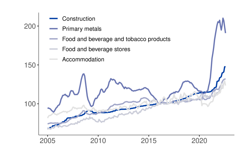
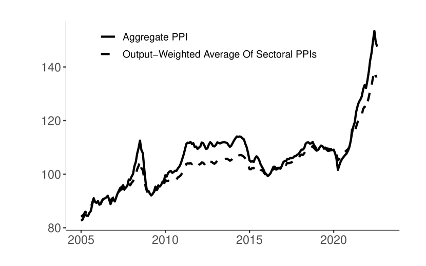
Figure 3: Sectoral and Aggregate PPI
Notes: The left panel shows the raw PPI series for a few selected sectors. The right panel compares the aggregate PPI from the FRED Database and the output-weighted average of PPIs of sectors included in the analysis.

Suggestive evidence that network proximity does not only have implications for the contemporaneous cross-sectional correlation of price changes across sectors, but also for dynamic correlations is provided in Fig. 4. The lightest-blue line plots the contemporaneous correlation of prices in two sectors against their distance(s). It reproduces for prices the finding in Carvalho (2014) that sectoral comovement decreases with the distance between sectors, although this relationship is much less pronounced at the higher level of disaggregation analyzed here. However, it is not only the contemporaneous comovement between sectors that decreases with distance, but also the comovement of sector $i$’s inflation with lagged values of sector $j$’s inflation is declining with the distance from sector $i$ to sector $j$. This is illustrated by the remaining lines in Fig. 4, which show this correlation for lags ranging from one to twelve months in darker shades of blue. In fact, the downward slope is more pronounced for higher lags.

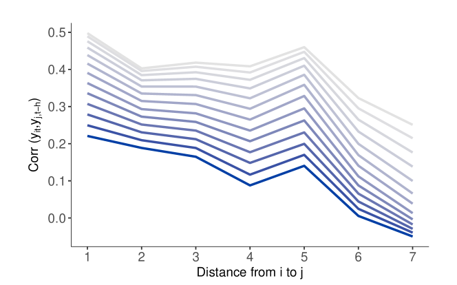
Figure 4: Network Distance and the Correlation of Sectoral Inflation
Notes: The figure plots the average correlation of sectoral prices for different distances between them. The lightest blue line refers to contemporaneous correlations. Darker lines show the average correlation of a sector $i$ with lagged values of a sector $j$ as a function of the distance from $i$ to $j$. Lags range from 0 to 12 months. The series refer to de-trended and de-seasonalized log PPIs.

4.3 Estimation

The theoretical analysis in Section 4.1 suggests that sectoral prices at some model-frequency evolve (approximately) as an NVAR($p,1$):

$$\tilde{y}_{\tau}=\alpha_{1}A\tilde{y}_{\tau-1}+...+\alpha_{p}A\tilde{y}_{\tau-p}+\tilde{u}_{\tau}\;.$$

Relative to the unconstrained estimation of $\alpha$ discussed in Section 3.1, the model from Section 4.1 restricts $\alpha_{l}\geq 0\;\forall\;l$ and $\sum_{l=1}^{p}\alpha_{l}=1$. To accommodate these restrictions, I drop $\alpha_{p}$ from $\alpha$ and impose the domain restrictions $\alpha_{l}\in[0,1]$ for $l=1:p-1$ and $\sum_{l=1}^{p-1}\alpha_{l}\leq 1$. For now, I assume that $\tilde{u}_{i\tau}$ is uncorrelated across $i$ and $\tau$ with $\tilde{u}_{i\tau}\sim N(0,\sigma_{i}^{2})$.

I consider Bayesian estimation of $\theta=(\alpha,\sigma)$ under Uniform priors for $\alpha=(\alpha_{1},..,\alpha_{p-1})$ and $\sigma=(\sigma_{1},...,\sigma_{n})$. As a result, the posterior mode is equal to the Maximum Likelihood Estimator. The prior for $\{\alpha_{l}\}_{l=1:p-1}\in[0,1]^{p-1}$ is truncated to satisfy the additional domain restriction $\sum_{l=1}^{p-1}\alpha_{l}\leq 1$. The posterior is obtained numerically using the Sequential Monte Carlo (SMC) algorithm. Details are in Section C.3.

I allow the frequency of network interactions to differ from the frequency of observation and infer their relation from the data by model selection criteria. As in Section 2.2.2, let $\{y_{t}\}_{t=1}^{T}=\{\tilde{y}_{qt}\}_{t=1}^{T}$ denote the observed series. I consider $q\in\{\frac{1}{3},\frac{1}{2},1,2,4\}$, which under monthly observations corresponds to quarterly, bi-monthly, monthly, bi-weekly and weekly network interactions, respectively. Also, I allow for lags up to 6 months to matter for dynamics.

4.4 Results

Table 1 reports the Marginal Data Density (MDD) for different specifications of the NVAR. The most preferred specification features monthly network interactions and lags up to six months. Model selection according to the Bayesian or Akaike Information Criteria lead to the same conclusion (see Table A-2). The subsequent analysis is based on this preferred NVAR($6,1$).

Table 1: Model Selection: Log MDD

		$p$
		$1q$	$2q$	$3q$	$4q$	$5q$	$6q$
	1/3			19079			19044
	1/2		19384		18768		18690
$q$	1	20153	20056	19675	19879	18899	20218
	2	17546	19570	19248	20142	18662	19636
	4	18517	19808	19754	19655	18904	19301
Notes: The table shows values for the natural logarithm of the Marginal Data Density (MDD) across model specifications. The values for $q$ (from top to bottom) refer to quarterly, bi-monthly, monthly, bi-weekly and weekly network interactions, respectively, while $p=mq$ implies that the last $m$ months matter for dynamics.

Table 2 reports the estimation results for $\alpha$. The first column shows the posterior mode or MLE, approximated by the Maximum A-Posteriori (MAP) estimator, i.e. the posterior draw (particle in the SMC algorithm) with the highest likelihood and posterior. It is very close to the posterior mean, reported in the second column. The tight 95% Highest Posterior Density (HPD) intervals – shown in columns three and four – together with the peaked marginal posteriors – shown in Fig. A-4 – illustrate that $\alpha$ is estimated very precisely. This is not surprising as there are $nT=51\cdot 206=10,506$ observations and only $n+p-1=56$ parameters.

Table 2: Estimation Results: $\alpha$

	MAP	Mean	Low	High
$\alpha_{1}$	0.1550	0.1557	0.1370	0.1745
$\alpha_{2}$	0.3460	0.3382	0.3168	0.3605
$\alpha_{3}$	0.2816	0.2865	0.2644	0.3129
$\alpha_{4}$	0.0915	0.0991	0.0785	0.1174
$\alpha_{5}$	0.1045	0.0975	0.0837	0.1135
Notes: The first column shows the Maximum Likelihood or Maximum A-Posteriori (MAP) Estimator, the second refers to the posterior mean, and Low and High report the bounds of the 95% Bayesian HPD credible sets.

The dynamics of $y_{t}$ can be summarized by impulse response functions (IRF). By Section 2.2, under an NVAR($6,1$), the impulse response of $y_{t}$ at horizon $h$ comprises supply chain connections of order $k\in\underline{k}:h$, with $\underline{k}=ceil(h/6)$:

$$\frac{\partial y_{i,t+h}}{\partial u_{j,t}}=\left[{\frac{\partial y_{t+h}}{\partial u_{t}}}\right]_{ij}=c^{h}_{\underline{k}}(\alpha)\left[{A^{\underline{k}}}\right]_{ij}+...+c^{h}_{h}(\alpha)\left[{A^{h}}\right]_{ij}\;.$$ (12)

The coefficients $\{c^{h}_{k}(\alpha)\}_{k=\underline{k}:h}$ are functions of $\alpha$ and show the importance of (upstream) supply chain connections of different order for the response of sectoral prices at any one horizon $h$. As the analysis abstracts from hetereogeneity in $\alpha$, these coefficients are constant across time and sector-pairs.

Fig. 5 illustrates this composition of impulse responses. The dots in the top left panel depict the coefficients $\{c^{h}_{k}\}_{k=\underline{k}:h}$ with horizons $h$ on the x-axis and connection-orders $k$ on the y-axis. Higher values are represented by larger and darker dots. As stated above, under $\alpha_{l}>0$ for $l=1:6$, orders $\underline{k}:h$ matter for propagation at horizon $h$. Hence, there are $h-\underline{k}+1$ dots aligned vertically at horizon $h$. As time passes, a shock spreads through the network and reaches more distant nodes. The estimated $\{\hat{\alpha}\}_{l=1:6}$ determine the exact width and speed of this propagation, illustrated by the differing sizes and colors of the dots.

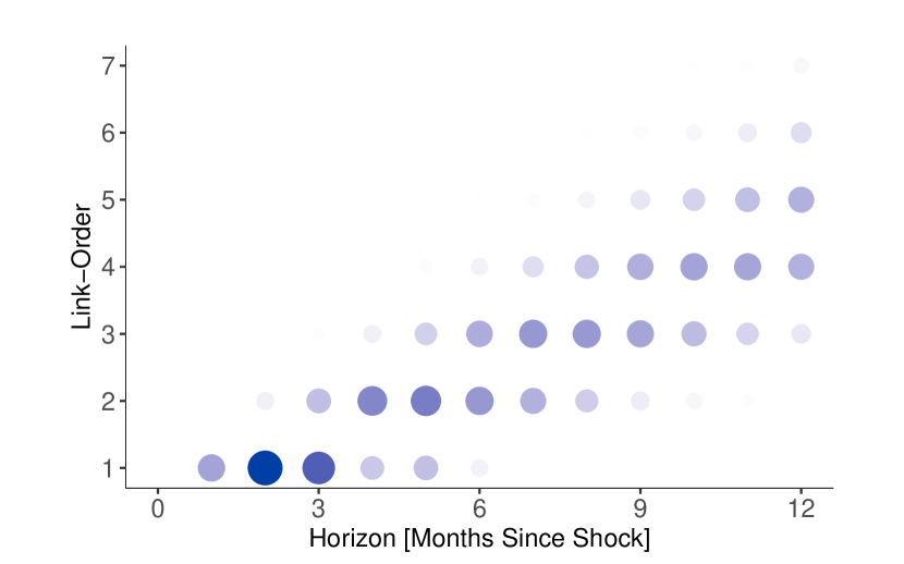
(a) Relevance of Link-Orders Across Horizons

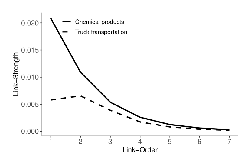
(b) Input-Output Links to Utilities Sector

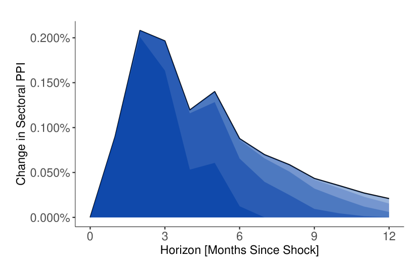
(c) IRF of Chemical Products to Utilities

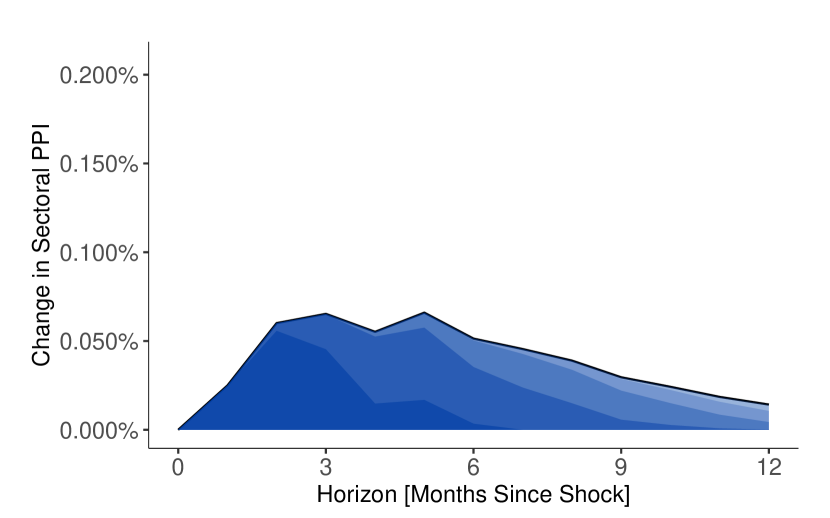
(d) IRF of Truck Transportation to Utilities

Figure 5: Impulse Responses: Transmission of Price Shocks via Supply-Chain Links
Notes: The top left panel shows the importance of different connection-orders for shock transmission as a function of the time elapsed since a shock took place. The top right panel shows the supply chain connections of different order from the sectors “Chemical Products” and “Truck Transportation” to the utilities sector, and the bottom panels show their resulting IRFs to an increase in the price of utilities by one standard deviation.

The top right panel in Fig. 5 shows the strength of network connections of different order from the sectors “Chemical Products” and “Truck Transportation” to the sector “Utilities”, respectively. The former sector is more dependent on utilities as a supplier than the latter, as evidenced by stronger network connections, in particular of first and second order. As Eq. 12 above makes clear, such network-connections are the second building block of impulse responses in the NVAR.

The lower panels of Fig. 5 illustrate the resulting impulse responses. The different shades of blue depict the individual terms $c^{h}_{k}(\alpha)\left[{A^{k}}\right]_{ij}$, which show the contribution of network-connections of order $k$ to the impulse-response of $i$ to $j$ at horizon $h$. Darker shades refer to network connections of lower order. As a result of its stronger network-connections to the utilities sector, the price of chemical products reacts more strongly to a one-standard deviation increase in the price of utilities than does the price of truck transportation. The price of chemicals rises quickly and peaks after two months. In contrast, the price of truck transportation increases slowly and remains slightly elevated without a noticeable peak. It is in particular the direct and second-order supply-chain connections that make up the difference between the two responses, in line with the top right panel. Longer-term responses are driven by higher-order connections and after nine months they are of similar size for the two sectors as they share similarly strong higher-order connections to the utilities sector.

Existing literature uses a static framework of contemporaneous input-output conversion which shows that the effects of sectoral TFP shocks on aggregate prices are stronger for sectors with more central positions in the supply chain network. As discussed in Section 2.2, because $\sum_{l=1}^{p}=1$, the effects under that framework are equal to the long-term responses of prices to permanent shocks in the present NVAR. As opposed to the static framework, the NVAR provides information on how the effects of a sectoral TFP shock on prices unfold over time. In the following, I focus on the responses of aggregate PPI, but the same analysis could be conducted for sector-pairs $(i,j)$.

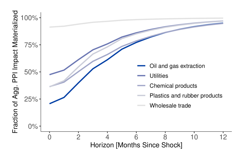
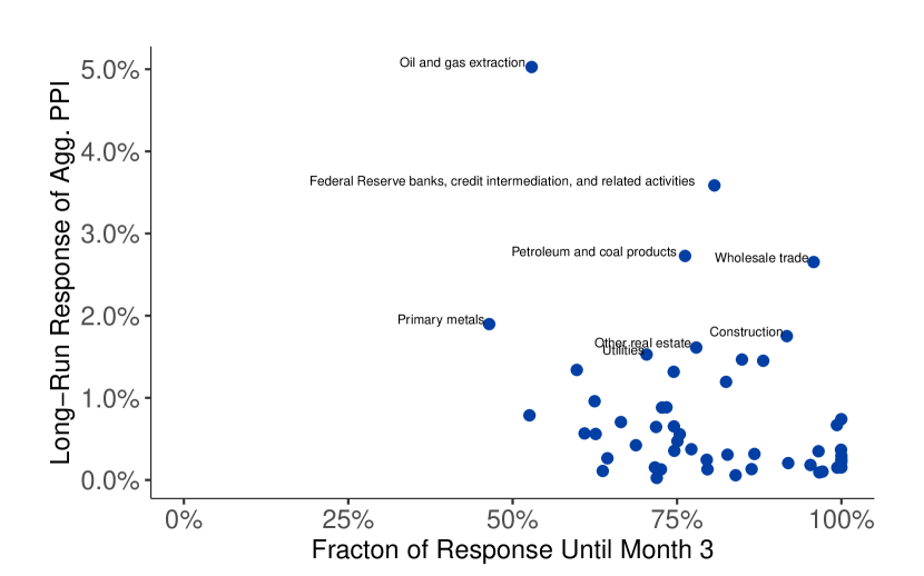
Figure 6: Size and Timing of Aggregate PPI Response to Sectoral Shocks
Notes: The left panel shows the time profile of the effect of sectoral price disturbances on aggregate PPI for a few selected sectors. The right panel relates the strength of the effect on aggregate PPI to its timing. The shock sizes are equal to one standard deviation of the respective sectoral disturbance.

The left panel of Fig. 6 shows the time profiles of aggregate PPI responses to price increases in different sectors. It suggests that sectors differ in the speed at which they impact aggregate PPI. For example, the response of aggregate PPI to a shock to wholesale trade prices materializes rather quickly, while its response to an increase in the price of oil and gas extraction takes time. As revealed by the IRF discussion above, this is because wholesale trade connects to other sectors mostly as a direct or lower-order supplier, while the oil and gas extraction sector sits further upstream in its supply-chain relationships. In case of the aggregate PPI, the relevant counterpart is a weighted average of customer-sectors, with weights given by their contribution to aggregate output.

The right panel of Fig. 6 plots the strength of aggregate PPI responses against the fractions which materialize during the first quarter after the shock. Although stronger effects tend to take more time to realize, there is no clear relationship between the strength and timing of responses. For example, the construction and primary metals sectors have similar long-term effects on aggregate prices because other sectors (or the output-weighted average of them) have similar “overall” connections to both, as judged by the sum of connections of all order in the Leontief inverse. Yet the impact of price increases in the construction sector materializes much more quickly since this sector is more relevant as an immediate supplier to relevant sectors in the economy compared to the primary metals sector.

In sum, the present analysis confirms the result from the existing literature that the stronger the connections from sector $i$ to sector $j$, the more pronounced is the response of sector $i$’s PPI to a price shock in sector $j$. In addition, the analysis suggests that how fast sector $i$ responds depends on the importance of sector $j$ as a more immediate – rather than further upstream – supplier to sector $i$. The exact mapping from network-connections to impulse responses is determined by the extent to which connections of different order matter at different horizons. This is true not only for prices in a sector $i$, but also for a weighted average of sectoral prices, such as the aggregate PPI.

5 Forecasting Global Industrial Production Growth

How does economic activity co-move across countries? Given an expansion in one country, how do we expect economic activity in other countries to react? The international economics literature has long been interested in spillover and spillback effects across countries and the transmission of US shocks in particular. In this section, I shed light on global business cycles from a novel perspective, by assuming that the dynamic comovement in economic activity across countries is the result of bilateral connections, which I estimate. This is in starkest contrast with factor models, which in this context posit that it is the result of exposure to a few influential economies.

The previous section examined a case where an observed cross-sectional time series is arguably driven by one particular network of bilateral links for which data is available, and the interest lies in quantifying how network effects materialize over time. In this section, I consider the case where no network data is available, yet the assumption of an underlying network structure that shapes (cross-sectional) dynamics appears reasonable. I first provide some intuition on the merits of the NVAR as a tool for approximating cross-sectional time series in Section 5.1 and discuss the relation to alternative methods. The application to cross-country industrial production growth is set up in Section 5.2, with results presented in Section 5.3.

5.1 Modeling Cross-Sectional Processes by Sparse Networks

Consider the problem of approximating dynamics of a cross-sectional time series $y_{t}$. Even for intermediate sizes of the cross-section, an unrestricted VAR($p$) is not feasible. Modeling the series as an NVAR($p,q$) process and estimating $(\alpha,A)$ gives a sparse, yet flexible and interpretable alternative.

Sparsity is obtained by the assumption that innovations transmit cross-sectionally only via bilateral links. As a result, the information in the high-dimensional vector of potential covariates – the lagged values of $y_{t}$ – is compressed into a low-dimensional vector of regressors $X_{t}$ that summarizes this information using network connections:

$$y_{t}=X_{t}\alpha+u_{t}\;,\quad X_{t}=[Ay_{t-1},...,Ay_{t-l}]\;.$$

Furthermore, because two units can be connected even in absence of a direct link between them, the dynamic, cross-sectional comovement may potentially be captured by relatively few non-zero bilateral links. In other words, $A$ can be sparse, leading to additional parsimony. Assuming that dynamic relations across all unit-pairs $(i,j)$ are driven by a relatively small set of bilateral links is akin to the assumption that longer-term dynamics are driven by a set of shorter-term dynamics, which is upheld by the general class of VARMA($p,q$) models.

Flexibility is obtained because the connections in $A$ are estimated and because the NVAR($p,q$) can capture rather general patterns of which connection-orders matter at which horizons, in particular for $q>1$. The VARMA process in Eq. 5, which approximates the dynamics of $y_{t}$ under an NVAR($p,q$) with $q>1$, brings to mind functional approximation of the linear projection of $y_{t}$ on the information set at $t-1$ using a polynomial expansion in $A$. Thereby, adding a term $\gamma_{lk}A^{k}$ to the equation satisfies the two main requirements on basis functions, orthogonality and locality: the term i) adds new, orthogonal information to that captured by lower powers of $A$, ii) adds different information across node-pairs $(i,j)$, and iii) adds this information only at lag $l$.

Comparison to Alternatives

There is a vast literature on modeling high-dimensional time series. The methods by which parsimony is induced can be roughly split into three categories. Variable selection methods like Lasso or boosting aim at finding the most important predictors by excluding less relevant ones. Instead of imposing outright exclusion restrictions, shrinkage methods such as Ridge regression or Minnesota-type priors do that by downweighting less relevant ones. Finally, factor models and reduced rank regression models reduce dimensionality by summarizing a large set of predictors by a few linear combinations of them.

The NVAR combines insights from factor models and shrinkage methods. Compared to factor models, it offers a particular way of finding the linear combination that effectively summarizes the information in the high-dimensional set of predictors $y_{t-1}^{\prime},y_{t-2}^{\prime},...$, namely by the set of bilateral links among cross-sectional units. Compared to shrinkage methods, the NVAR applies regularization to bilateral links $a_{ij}$, which in turn summarize the information in the predictors at all lags. As a result, it entertains the additional sparsity assumption that, for any variable $i$, the same linear combinations of predictor-variables $j$ matter at all lags $l=1:p$. Nevertheless, dynamics at different horizons $h$ are driven by different linear combinations, i.e. different sets of connection-orders, even more so if the network interaction frequency is allowed to be higher than the frequency of observation (see Proposition 1 and discussion in Section 2.2.2). This additional restriction can become important in higher dimensions.

The rank of the network adjacency matrix $A$ in the NVAR($p,1$) is related to the number of factors in a factor model, arguably the most popular method for modeling high dimensional time series in macroeconomics. It is easy to see that an NVAR($p,1$) permits a factor structure, with the number of factors given by the number of non-redundant columns in $A$. The equivalence result in Section D.1 establishes in addition that, for large $n$, a factor model can be cast as an NVAR($p,1$) – with the number of factors again equal to the rank of $A$ – provided that the factors themselves evolve according to an NVAR($p,1$). Note that for $p=1$, the latter condition just requires the factors to evolve according to a VAR($1$), while in case of a single factor, it requires the factor to follow an AR($p$).

Based on these insights, the NVAR is expected to better capture cross-sectional dynamics when these are composed of many (seemingly neglibile) links rather than driven by a few influential units. And indeed, in many cases, we expect $A$ to be sparse, yet of close-to-full rank. For example, most countries trade only with a subset of other countries, but act as a significant trading partner to at least one other country. Similarly, most sectors supply only a small subset of other sectors in the economy, yet for most sectors we can find at least one other sector whose output or price-setting behavior critically depends on that of the sector in question. In principle, the same can apply not only for units in cross-sectional time series, but for variables in multivariate time series more generally.

Regardless of the rank of $A$, the NVAR is expected to better capture the dynamics of $y_{it}$ for units $i$ with a dependence structure in $A_{i\cdot}$ (or factor loadings) that differs considerably from that of other units. As pointed out in Boivin and Ng (2006), the more dispersion there is in the factor loadings across series, the worse will be the forecasting performance of a factor model. This dispersion notably includes the case of weak factors, as captured by a sparse loading matrix (or a sparse adjacency matrix $A$ in the case of an NVAR). The NVAR naturally incorporates weak factors as locally important units in the network. Moreover, under the NVAR, sparsity of $A$ leads not only to cross-sectional differences in the strength of exposure to some given unit, but also to differences in the timing of this exposure. Therefore, the NVAR is further preferred to factor models whenever some notion of cross-sectional distance is expected to be relevant for the timing of impulse responses.

Even in case the NVAR offers no advantage to factor models in terms of modeling and forecasting cross-sectional dynamics, it may be preferred for other reasons. First, it estimates a network as relevant for dynamics and, relatedly, offers an interpretable way of approximating the dynamics in $y_{t}$. Second, it facilitates the analysis of spillover and spillback effects as it estimates the whole set of bilateral Granger-causality patterns. Third, the estimated network offers a possible method for shock identification in high dimensions, the assumption being that the same bilateral links that rationalize lagged innovation transmission are also behind contemporaneous shock transmission.

5.2 Forecasting Setup

I use the NVAR to model the dynamics of monthly industrial production (IP) growth across countries. IP data is obtained from the IMF and OECD databases. Based on the raw data, I compute growth rates relative to the same month a year ago. Data availability narrows the sample to 44 countries and the time frame January 2001 to July 2022. In all of the following, I limit the analysis to pre-COVID-19. The data is summarized in Table A-3 in Section D.2.

To assess forecasting performance, I first estimate an NVAR($p,1$) as well as a factor model based on data from January 2001 to December 2017 and consider out-of-sample forecasting performance for horizons up to 24 months ahead. The sample is iteratively increased by one month and the analysis is repeated until the sample end date reaches December 2019. Forecasts for periods after January 2020 are excluded from the assessment.

I estimate the NVAR($p,1$) enforcing $a_{ij}\geq 0$ and using a Lasso-penalty to shrink links in $A$ to zero (see Section 3.2). I select the optimal degree of sparsity in $A$ based on BIC by counting the number of non-zero elements in $\hat{A}(\lambda)$, as suggested in Zou et al. (2007). Once the NVAR is estimated, forecasts are obtained in the same way as for any VAR($p$) model. The factor model is estimated using principal components. I select the number of factors based on the information criterion developed in Bai and Ng (2002). To construct forecasts, I fit a VAR($p$) for the factors.

5.3 Results

The results of the forecasting exercise are shown in Fig. 7. It reports the average out-of-sample Mean Squared Error (MSE) across countries under the estimated NVAR($4,1$) relative to those obtained under the factor model. The NVAR($4,1$) yields a substantial reduction in MSE compared to the factor model. This holds in particular for forecasts up to six months ahead. The results for alternative choices of $p$ are similar (see Fig. A-6).

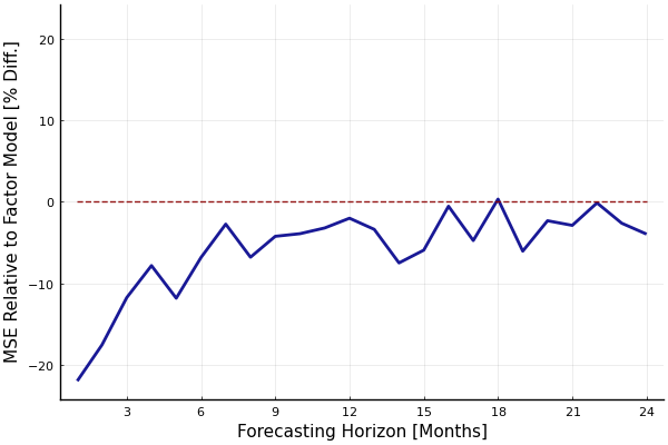
Figure 7: Out-of-Sample Forecasting Performance: NVAR($4,1$) vs. Factor Model
Notes: The plot depicts the percentage difference between the out-of-sample Mean Squared Errors generated by the NVAR($1,1$) to those generated by the Principal Components Factor Model.

On top of the good forecasting performance, the NVAR estimates the network as relevant for IP dynamics and the full set of Granger-causality patterns among units. The following discussion is based on the estimated network using data from January 2001 to December 2017 and setting $\lambda=0$. Note that even in this case, the estimated $A$ is sparse as $a_{ij}\in\mathbb{R}_{+}$ is enforced. In the network, 22% of the links are non-zero. Excluding links below 0.05, the network density drops to 11%. Nevertheless, $\hat{A}$ has rank 38 and is therefore close to full-rank. For higher values of $\lambda$, selected as optimal by BIC and used to construct the forecasts in Fig. 7, this number is lower, but always stays at levels that exceed the factor dimensions commonly selected in applications.

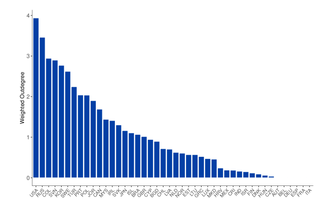
Figure 8: Weighted Out-degrees in the Estimated Network
Notes: The plot depicts the weighted outdegrees in the estimated network as relevant for monthly industrial production dynamics across countries.

Fig. 8 shows weighted out-degrees, $\hat{wd}^{j}_{out}=\sum_{i}\hat{a}_{ij}$, a measure of country $j$’s influence on IP dynamics of other countries in the sample. Without any information beyond the IP series across countries, the NVAR estimates the most influential country to be the United States, in line with expectations. The second most influential country is Russia, another large economy and major energy-exporter. The ordering of countries according to this measure does also show some surprises. In particular, Germany, France and Italy are estimated to not influence any other country in the sample. This is presumably due to high (contemporaneous) correlation of economic activity among countries in the Euro Area and EU. As a result, the model likely attributes innovations coming from these three major European economies to Slovenia, Sweden, Portugal and Poland, all of which are estimated to be among the most influential countries. Such results can be avoided by including prior information. For example, one could shrink links to some measure of bilateral connection from the data, such as capital or trade flows.

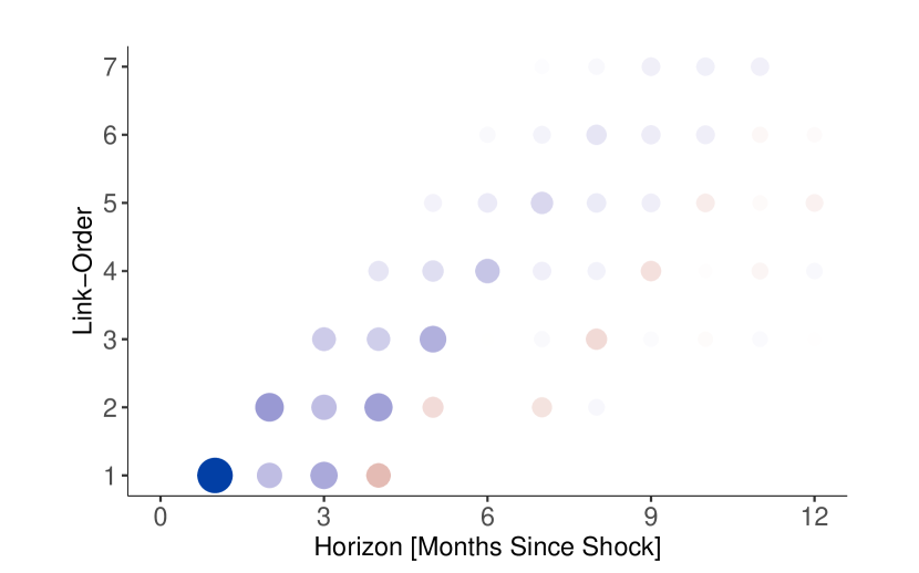
(a) Relevance of Link-Orders Across Horizons

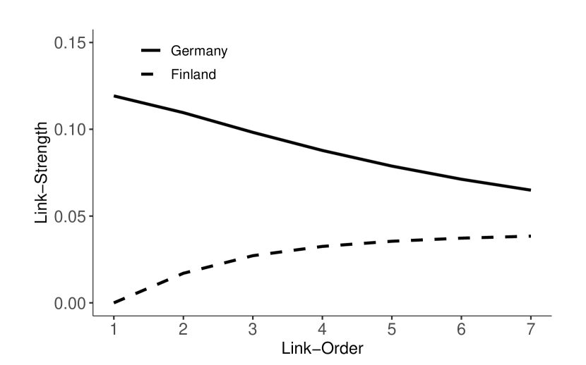
(b) Links to United States

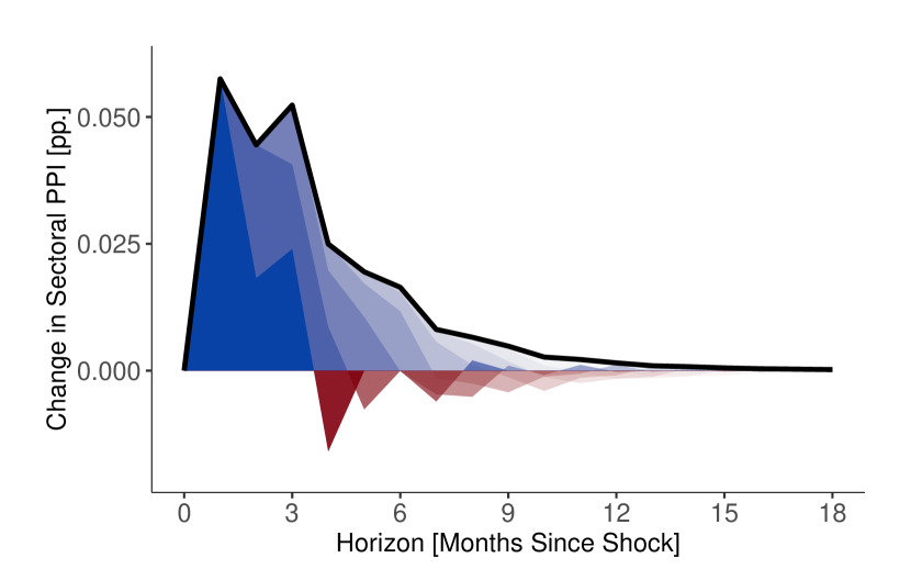
(c) IRF of Germany to United States

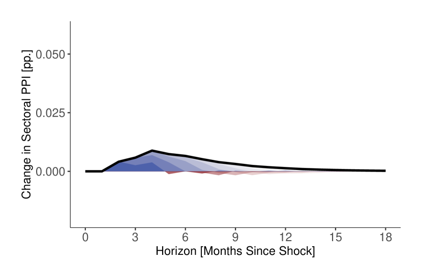
(d) IRF of Finland to United States

Figure 9: Impulse Responses: Network-Induced Transmission of Economic Activity
Notes: The top left panel shows the importance of different connection-orders for transmission as a function of the time elapsed since an innovation took place. The top right panel shows the connections of all order from Germany and Finland to the United States, and the bottom panels show their resulting IRFs to a one standard deviation increase in US industrial production.

In the top left panel of Fig. 9, I illustrate the propagation pattern of innovations to IP growth through the network as captured by $\hat{\alpha}$. As in Fig. 5 in Section 4, the dots show which connection orders matter for innovation propagation at which horizon, with the strength reflected by the dots’ size and shading. In contrast to Fig. 5, however, the coefficients in $\alpha$ are not restricted to be positive in this application. To distinguish positive from negative transmission, I show the former in blue and the latter in red. The plot suggests that following an incrase in a country’s IP growth, other countries’ response features an initial overshooting and subsequent correction. The exact magnitudes of these forces depend on network connections of different order between any given pair $(i,j)$. The top right panel of Fig. 9 reports these connections from Germany and Finland, respectively, to the United States. While Germany is estimated to have a strong direct link to the US, the dependence of Finnish IP on that of the US comes only from higher-order connections and is weaker overall. As a result, the lower panels of Fig. 9 show that IP in Germany responds much faster and stronger to an increase in US IP growth. In contrast, it takes time for this increase to travel through the network and affect economic activity in Finland. Both impulse responses show a sinusoidal pattern of innovation transmission via any one given order of network connections, reflecting the initial overshooting and subsequent correction. This is depicted by different shading for different link-orders.

6 Conclusion

In this paper, I develop an econometric framework that explicitly relates the dynamics of cross-sectional variables to the bilateral links among cross-sectional units. In a first application, I use it to estimate how supply chain linkages affect the dynamics of sectoral prices in the US economy. In a second application, I apply it as a dimensionality-reduction technique for modeling cross-country industrial production growth.

As discussed in the introduction, most existing studies in macroeconomics establish relations between network statistics and cross-sectional properties in static environments. The proposed NVAR can be used to examine the relation between network properties and cross-sectional dynamics, avoiding the simplifying assumption of contemporaneous network interactions. Thereby, the model could be augmented to accommodate heterogeneous propagation patterns across units or over time. By adding covariates, it could assess to what extent dynamics are driven by a particular network as opposed to other forces.

The NVAR presented in this chapter assumes that innovation transmission occurs along bilateral links which are fixed over time. An important methodological step forward would be to develop a tractable framework that links such network effects to network formation. In many cases, units can adjust their network position in reaction of innovations transmitted through the network.

A further promising direction for future research is the use of networks - estimated or not - for shock identification. This possibly offers a solution to the challenge of finding a convincing identification strategy for cross-sectional time series, in particular under high dimensions.

Appendix A NVAR Model

A.1 Granger-Causality

Proposition 2 (Granger-Causality in NVAR($p,1$)).

Let $y_{t}$ follow an NVAR(p,1):

$$y_{t}=\sum_{l=1}^{p}\Phi_{l}y_{t-l}+u_{t}\;,\quad\Phi_{l}=\alpha_{l}A\;,\quad\alpha_{l}\in\mathbb{R}\;,$$

and assume $\alpha_{l}\neq 0$ for $l=1:p,$. Then $\frac{\partial y_{i,t+h}}{\partial y_{j,t}}>0\Leftrightarrow(A^{k})_{ij}>0$ for at least one $k\in\underline{k}:h$, $\underline{k}=ceil(h/p)$, i.e. $y_{j}$ Granger-causes $y_{i}$ at horizon $h$ if and only if there exists a walk from $i$ to $j$ of at least one length $k\in\underline{k}:h$.

Proof: Using the companion form of this process, we have

$$\frac{\partial y_{t+h}}{\partial y_{t}} =[I_{n},0_{n\times n(p-1)}]F^{h}[I_{n},0_{n\times n(p-1)}]^{\prime}=(F^{h})_{11}\;,$$

$$F =\begin{bmatrix}\Phi_{1}&\Phi_{2}&...&\Phi_{p-1}&\Phi_{p}\\ I_{n}&0_{n}&...&0_{n}&0_{n}\\ 0_{n}&I_{n}&...&0_{n}&0_{n}\\ \vdots&&\ddots&&\vdots\\ 0_{n}&0_{n}&...&I_{n}&0_{n}\end{bmatrix}\;,\quad\Phi_{l}=\alpha_{l}A\;.$$

I will prove the following claim by induction: $(F^{h})_{1l}$, the $n\times n$ matrix in position $(1,l)$ of the $np\times np$ matrix F, has powers of $A$ in the set $ceil(\frac{h+l-1}{p}):h$. Note that the claim is true for $h=1$. Assume it is true for $h$. For $h+1$ we have

$$F^{h+1} =\begin{bmatrix}(F^{h})_{11}&(F^{h})_{12}&...&(F^{h})_{1p}\\ (F^{h})_{21}&(F^{h})_{22}&...&(F^{h})_{2p}\\ \vdots&&\ddots&\vdots\\ (F^{h})_{p1}&(F^{h})_{p2}&...&(F^{h})_{pp}\end{bmatrix}\begin{bmatrix}\Phi_{1}&\Phi_{2}&...&\Phi_{p-1}&\Phi_{p}\\ I_{n}&0_{n}&...&0_{n}&0_{n}\\ 0_{n}&I_{n}&...&0_{n}&0_{n}\\ \vdots&&\ddots&&\vdots\\ 0_{n}&0_{n}&...&I_{n}&0_{n}\end{bmatrix}$$

$$=\begin{bmatrix}(F^{h})_{11}\Phi_{1}+(F^{h})_{12}&(F^{h})_{11}\Phi_{2}+(F^{h})_{13}&...&(F^{h})_{11}\Phi_{p-1}+(F^{h})_{1p}&(F^{h})_{11}\Phi_{p}\\ \vdots&\vdots&\ddots&\vdots&\vdots\end{bmatrix}\;,$$

where I only show the first row of blocks in $F^{h+1}$ as only they are relevant to the argument.

Let $h+m$ for some $m\in 1:p-1$ be a multiple of $p$ such that $ceil(\frac{h+l-1}{p})=\frac{h+m}{p}$ for $l=1:m+1$, while $ceil(\frac{h+l-1}{p})=\frac{h+m}{p}+1$ for $l=m+2:p$. This means that $(F^{h})_{1l}$ for $l=1:m+1$ have powers of $A$ in $\frac{h+m}{p}:h$, while $(F^{h})_{1l}$ for $l=m+2:p$ have powers in $\frac{h+m}{p}+1:h$. Then, using the equation above, $(F^{h+1})_{1l}$ for $l=1:m$ have powers of $A$ in $\frac{h+m}{p}:h+1=ceil(\frac{h+1+l-1}{p}):h+1$, while $(F^{h+1})_{1l}$ for $l=1:m$ have powers in $\frac{h+m}{p}+1:h+1=ceil(\frac{h+1+l-1}{p}):h+1$. Note that these sets are independent of $m$ and therefore the claim holds for $h+1$ in all possible cases. $\blacksquare$

A.2 Time-Aggregation of Lagged Transmission Patterns

In this section, I show that the state space representations in Eq. 4 and Eq. 6 for $q\in\mathbb{N}\backslash\{1\}$ lead to a VARMA process for the observed series $\{y_{t}\}_{t=1}^{T}$ of the type of Eq. 5. For illustration purposes, let $\tilde{y}_{\tau}$ follow an NVAR($3,1$).

Suppose $\tilde{y}_{\tau}$ is a stock variable observed every $q=2$ periods. Under monthly observations, this means that network interactions happen bi-weekly. Suppose the particular realization at period $\tau$, $\tilde{y}_{\tau}$, is observed. Inserting sequentially for the non-observed $\tilde{y}_{\tau-1}$ and $\tilde{y}_{\tau-3}$, we get

$$\tilde{y}_{\tau} =\left[{\alpha_{2}A+\alpha_{1}^{2}A^{2}}\right]\tilde{y}_{\tau-2}+\left[{(\alpha_{1}\alpha_{2}+2\alpha_{1}\alpha_{3})A^{2}}\right]\tilde{y}_{\tau-4}$$

$$\quad+\tilde{u}_{\tau}+\alpha_{1}A\tilde{u}_{\tau-1}+(\alpha_{3}A+\alpha_{1}\alpha_{2}A^{2})\tilde{u}_{\tau-3}+\text{terms in }\tilde{y}_{\tau-6},\tilde{y}_{\tau-7}\;.$$

This can be written (for a generic observational period $t$) as

$$y_{t}=\Phi_{1}y_{t-1}+\Phi_{2}y_{t-2}+\Theta_{0}\eta_{t}+\Theta_{1}\eta_{t-1}+\text{terms in }\tilde{y}_{\tau-6},\tilde{y}_{\tau-7}\;,$$

where $y_{t-l}=\tilde{y}_{\tau-2l}$ for $l=0,1,2$, $\eta_{t}=[\tilde{u}_{\tau}^{\prime},\tilde{u}_{\tau-1}^{\prime}]^{\prime}$, $\eta_{t-1}=[\tilde{u}_{\tau-2}^{\prime},\tilde{u}_{\tau-3}^{\prime}]^{\prime}$, and

$$\Phi_{1}=\alpha_{2}A+\alpha_{1}^{2}A^{2}\;,\quad\Phi_{2}=(\alpha_{1}\alpha_{2}+2\alpha_{1}\alpha_{3})A^{2}\;,\quad\Theta_{0}=\left[{I_{n},\alpha_{1}A}\right]\;,\quad\Theta_{1}=\left[{0_{n},\alpha_{3}A+\alpha_{1}\alpha_{2}A^{2}}\right]\;.$$

The exact process $\{y_{t}\}_{t=1}^{T}=\{\tilde{y}_{qt}\}_{t=1}^{T}$ contains infinitely many lags with ever higher powers of $A$ at higher lags. However, if $\tilde{y}_{\tau}$ is stationary, then so is $y_{t}$ and the latter can be approximated with some finite number of lags $p^{*}$.

Suppose instead that $\tilde{y}_{\tau}$ is a flow variable and we observe $y_{\tau/2}=\tilde{y}_{\tau}+\tilde{y}_{\tau-1}$ for $\tau/2\in\mathbb{N}$. Starting from $y_{t}=\tilde{y}_{\tau}+\tilde{y}_{\tau-1}$, iteratively inserting for $\tilde{y}_{\tau}$ and $\tilde{y}_{\tau-1}$ and adding and subtracting an $\tilde{y}_{\tau-3}$-term so as to align the coefficients in front of $\tilde{y}_{\tau-2}$ and $\tilde{y}_{\tau-3}$, we obtain

$$y_{t} =\tilde{y}_{\tau}+\tilde{y}_{\tau-1}$$

$$=[(\alpha_{1}+\alpha_{2})A+\alpha_{1}^{2}A^{2}](\tilde{y}_{\tau-2}+\tilde{y}_{\tau-3})+\tilde{u}_{\tau}+[I+\alpha_{1}A]\tilde{u}_{\tau-1}$$

$$\quad+[(\alpha_{3}-\alpha_{1})A+\alpha_{1}(\alpha_{2}-\alpha_{1})A^{2}]\tilde{y}_{\tau-3}+[\alpha_{3}A+\alpha_{1}\alpha_{3}A^{2}]\tilde{y}_{\tau-4}\;.$$

Inserting for the terms in the second row and adding and subtracting a $\tilde{y}_{\tau-5}$-term, we get

$$y_{t} =\tilde{y}_{\tau}+\tilde{y}_{\tau-1}$$

$$=[(\alpha_{1}+\alpha_{2})A+\alpha_{1}^{2}A^{2}](\tilde{y}_{\tau-2}+\tilde{y}_{\tau-3})+\tilde{u}_{\tau}+[I+\alpha_{1}A]\tilde{u}_{\tau-1}+[(\alpha_{3}-\alpha_{1})A+\alpha_{1}(\alpha_{2}-\alpha_{1})A^{2}]\tilde{u}_{\tau-3}$$

$$\quad+[\alpha_{3}A+\alpha_{1}(2\alpha_{3}-\alpha_{1})A^{2}+\alpha_{1}^{2}(\alpha_{2}-\alpha_{1})A^{3}](\tilde{y}_{\tau-4}+\tilde{y}_{\tau-5})+\text{terms in }\tilde{y}_{\tau-5},\tilde{y}_{\tau-6}\;,$$

which can be written as

$$y_{t}=\Phi_{1}y_{t-1}+\Phi_{2}y_{t-2}+\Theta_{0}\eta_{t}+\Theta_{1}\eta_{t-1}+\text{terms in }\tilde{y}_{\tau-5},\tilde{y}_{\tau-6}\;,$$

where $y_{t-l}=\tilde{y}_{\tau-2l}+\tilde{y}_{\tau-2l-1}$ for $l=0,1,2$, $\eta_{t}=[\tilde{u}_{\tau}^{\prime},\tilde{u}_{\tau-1}^{\prime}]^{\prime}$, $\eta_{t-1}=[\tilde{u}_{\tau-2}^{\prime},\tilde{u}_{\tau-3}^{\prime}]^{\prime}$, and

$$\Phi_{1} =(\alpha_{1}+\alpha_{2})A+\alpha_{1}^{2}A^{2}\;,\quad\Phi_{2}=\alpha_{3}A+\alpha_{1}(2\alpha_{3}-\alpha_{1})A^{2}+\alpha_{1}^{2}(\alpha_{2}-\alpha_{1})A^{3}\;,$$

$$\Theta_{0} =\left[{I_{n},I+\alpha_{1}A}\right]\;,\quad\Theta_{1}=\left[{0_{n},(\alpha_{3}-\alpha_{1})A+\alpha_{1}(\alpha_{2}-\alpha_{1})A^{2}}\right]\;.$$

As in the case of stock variables, the exact process $\{y_{t}\}_{t=1}^{T}$ contains infinitely many lags with ever higher powers of $A$ at higher lags. However, if $\tilde{y}_{\tau}$ is stationary, then so is $y_{t}$ and the latter can be approximated well with a finite number of lags.

Both for stock and flow variables, the procedure of finding the coefficient matrices $\{\Phi_{l}\}_{l=1}^{p}$ and $\{\Theta_{l}\}_{l=0}^{p-1}$ in the approximating VARMA-representation can be formalized as an algorithm for general $p$ and $q$. However, this does not offer any benefits in terms of estimation or model analysis relative to the state space representations in Eq. 4 and Eq. 6.

In Eq. 5, $q^{*}$ is claimed to be equal to $p^{*}q$. This is because the largest power of $A$ in any $\Phi_{l}$ cannot exceed $p^{*}q$ (and the coefficients $\gamma_{lg}$ can be zero). To see this, note that starting from the equation for $\tilde{y}_{\tau}$ and iteratively inserting for all $\tilde{y}_{\tau-j},j=1:h-1$, one would obtain $\partial\tilde{y}_{\tau+h}/\partial\tilde{y}_{\tau}$ as the coefficient-matrix in front of $\tilde{y}_{\tau-h}$, which we know consists of powers of $A$ in the set $k\leq h$. However, when performing the time-aggregation for stock variables, every $q$th $\tilde{y}_{\tau}$ is not inserted for, which means that powers accumulate slower. As a result, the coefficient-matrix in front of $y_{t-l}=\tilde{y}_{(t-l)q}$ contains powers not higher than $lq$. This is maximized for $l=p^{*}$. The same result applies also to flow variables.

The main text discusses the relation between network connections and impulse responses in the observed process for stock variables. For flow variables – $y_{t}=\tilde{y}_{\tau}+...+\tilde{y}_{\tau-q+1}$ for $\tau=tq$ with $q\in\mathbb{N}\backslash\{1\}$ – we get that $\partial y_{t+h}/\partial y_{t}$ can be composed of network-connections of order $k\in\{ceil((q(h-1)+1)/p),...,hq\}$, depending on which of the terms in $y_{t}=\tilde{y}_{tq}+...+\tilde{y}_{q(t-1)+1}$ is responsible for the change in $y_{t}$. If it is the first term, we get

$$\frac{\partial y_{t+h}}{\partial\tilde{y}_{tq}}=\frac{\partial(\tilde{y}_{(t+h)q}+...+\tilde{y}_{(t+h)q-q+1})}{\partial\tilde{y}_{tq}}=\frac{\partial\tilde{y}_{\tau+hq}}{\partial\tilde{y}_{\tau}}+...+\frac{\partial\tilde{y}_{\tau+hq-q+1}}{\partial\tilde{y}_{\tau}}$$

and so connection-orders $k\in\{ceil((q(h-1)+1)/p),...,hq\}$ matter. Analogous calculations show that if it is the last term, connection-orders $k\in\{ceil(hq/p),...,hq+q-1\}$ matter. For the response to contemporaneous innovations, $\partial y_{t}/\partial\eta_{t}$, connections of order $k\leq q-1$ can matter, depending on which of the terms $\tilde{u}_{tq},...,\tilde{u}_{tq-q+1}$ is behind the change in $\eta_{t}$.This is like for stock variables, but with the following subtle change. If it is the first term, then network-connections do not matter: $k\in\emptyset$. If it is the second term, then only first-order connections matter: $k\in\{ceil(1/p),...,1\}\cup\emptyset=\{1\}$. If it is the third term, then connections of order $k\in\{ceil(2/p),...,2\}\cup\{ceil(1/p),...,1\}\cup\emptyset=\{1,2\}$ matter. If it is the last term, then connections of order $k\in\{1,...,q-1\}$ matter.

A.3 Stationarity

Proposition 3 (Stationarity of NVAR($1,1$)).

Let $y_{t}$ follow an NVAR(1,1):

$$y_{t}=aAy_{t-1}+u_{t}\;,\quad a\in\mathbb{R}\;,$$

with $u_{t}\sim WN$ and assume $a\neq 0$. Then $y_{t}$ is weakly stationary iff for all eigenvalues $\lambda_{i}$ of $A$ it holds that $|\lambda_{i}|<1/|a|$.

Proof: This follows directly from the fact that $\lambda_{i}$ is an eigenvalue of $A$ iff $a\lambda_{i}$ is an eigenvalue of $aA$. Formally, let

$$\mathcal{L}_{A} =\left\{{\lambda_{i}:|\lambda_{i}I-A|=0}\right\}\;,$$

$$\mathcal{L} =\left\{{l_{i}:|l_{i}I-aA|=0}\right\}\;.$$

We have

$$y_{t}\;\text{weakly stationary}\quad\Leftrightarrow\quad \forall\;l_{i}\in\mathcal{L}\;,\quad|l_{i}|<1$$

$$\Leftrightarrow\quad \forall\;l_{i}\in\mathcal{L}\;,\quad|l_{i}/a|=|l_{i}|/|a|<1/|a|$$

$$\Leftrightarrow\quad \forall\;\lambda_{i}\in\mathcal{L}_{A}\;,\quad|\lambda_{i}|<1/|a|\;,$$

where the last equivalence follows from

$$|l_{i}I-aA|=|a(l_{i}/aI-A)|=a^{n}|l_{i}/aI-A|=0\Leftrightarrow|l_{i}/aI-A|=0\;.\quad\blacksquare$$

Proposition 4.

Let $y_{t}$ follow an NVAR($p,1$):

$$y_{t}=\alpha_{1}Ay_{t-1}+...+\alpha_{p}Ay_{t-p}+u_{t}\;,$$

with $u_{t}\sim WN$, and assume $\alpha_{l}\neq 0$ for at least one $l$. Define $a=\sum_{l=1}^{p}|\alpha_{l}|$, and let

$$y^{*}_{t}=aAy^{*}_{t-1}+u^{*}_{t}\;.$$

Then, $y_{t}$ is weakly stationary if $y^{*}_{t}$ is weakly stationary.

Proof: Let

$$\mathcal{Z} =\left\{{z_{i}:|I-\alpha_{1}Az_{i}-...-\alpha_{p}Az_{i}^{p}|=|I-(\alpha_{1}z_{i}+...+\alpha_{p}z_{i}^{p})A|=0}\right\}\;,$$

$$\mathcal{Z}^{*} =\left\{{z^{*}_{i}:|I-z^{*}_{i}aA|=0}\right\}\;.$$

The proof shall show

$$\forall\;z^{*}_{i}\in\mathcal{Z}^{*},\quad|z^{*}_{i}|>1\quad\Rightarrow\quad\forall\;z_{i}\in\mathcal{Z},\quad|z_{i}|>1\;.$$

We have

$$\forall\;z^{*}_{i}\in\mathcal{Z}^{*}\;,\quad|z^{*}_{i}|>1$$

$$\Leftrightarrow\quad \forall\;z^{*}_{i}\in\mathcal{Z}^{*},\quad|az^{*}_{i}|=a|z^{*}_{i}|>a$$

$$\Leftrightarrow\quad \forall\;z_{i}\in\mathcal{Z}\;,\quad|\alpha_{1}z_{i}+...+\alpha_{p}z_{i}^{p}|>a$$

$$\Rightarrow\quad \forall\;z_{i}\in\mathcal{Z}\;,\quad|z_{i}|>1\;.$$

To show the last implication, suppose first that the statement on the second-last line is true, but the statement on the last line is not. Then $\exists z_{i}\in\mathcal{Z}$ s.t. $|z_{i}|\leq 1$. In turn,

$$|\alpha_{1}z_{i}+...+\alpha_{p}z_{i}^{p}|\leq|\alpha_{1}z_{i}|+...+|\alpha_{p}z_{i}^{p}|\leq|\alpha_{1}z_{i}|+...+|\alpha_{p}z_{i}|\leq(|\alpha_{1}|+...+|\alpha_{p}|)|z_{i}|=a|z_{i}|\leq a\;,$$

a contradiction. $\blacksquare$

Proposition 5.

Let $y_{t}$ follow an NVAR($p,1$):

$$y_{t}=\alpha_{1}Ay_{t-1}+...+\alpha_{p}Ay_{t-p}+u_{t}\;,$$

with $u_{t}\sim WN$, and assume $\alpha_{l}\geq 0$ for $l=1:p$ and $\alpha_{l}>0$ for at least one $l$. Define $a=\sum_{l=1}^{p}\alpha_{l}$, and let

$$y^{*}_{t}=aAy^{*}_{t-1}+u^{*}_{t}\;.$$

Then, $y_{t}$ is weakly stationary iff $y^{*}_{t}$ is weakly stationary.

Proof: The proof is equivalent to that of Proposition 4, except that if $\alpha_{l}\geq 0\;\forall\;l$, the last implication is both-sided:

$$\forall\;z_{i}\in\mathcal{Z}\;,\quad|z_{i}|>1$$

$$\Rightarrow\quad \forall\;z_{i}\in\mathcal{Z}\;,\quad|\alpha_{1}z_{i}+...+\alpha_{p}z_{i}^{p}|>|(\alpha_{1}+...+\alpha_{p})z_{i}|=|az_{i}|=a|z_{i}|>a\;.\quad\blacksquare$$

Corollary 1 (Stationarity of NVAR($p,1$) I).

Let $y_{t}$ follow an NVAR($p,1$):

$$y_{t}=\alpha_{1}Ay_{t-1}+...+\alpha_{p}Ay_{t-p}+u_{t}\;,$$

with $u_{t}\sim WN$, and assume $\alpha_{l}\neq 0$ for at least one $l$. Define $a=\sum_{l=1}^{p}|\alpha_{l}|$.

Then $y_{t}$ is weakly stationary if for all eigenvalues $\lambda_{i}$ of $A$ it holds that $|\lambda_{i}|<1/a$.

If in addition $\alpha_{l}\geq 0\;\forall\;l$, then this condition is both necessary and sufficient.

Proposition 6 (Stationarity of NVAR($p,1$) II).

Let $y_{t}$ follow an NVAR($p,1$):

$$y_{t}=\alpha_{1}Ay_{t-1}+...+\alpha_{p}Ay_{t-p}+u_{t}\;,$$

with $u_{t}\sim WN$ and $\alpha_{l}\neq 0$ for at least one $l$.

Then, $y_{t}$ is weakly stationary iff the univariate AR(p) process

$$x_{t}=\lambda_{i}\alpha_{1}x_{t-1}+...+\lambda_{i}\alpha_{p}x_{t-p}+v_{t}$$

is weakly stationary for all eigenvalues $\lambda_{i}$ of $A$.

Proof: Stationarity of $y_{t}$ is equivalent to the statement that for all eigenvalues $l_{i}$ of

$$F =\begin{bmatrix}\alpha_{1}A&\alpha_{2}A&...&\alpha_{p-1}A&\alpha_{p}A\\ I_{n}&0_{n}&...&0_{n}&0_{n}\\ 0_{n}&I_{n}&...&0_{n}&0_{n}\\ \vdots&&\ddots&&\vdots\\ 0_{n}&0_{n}&...&I_{n}&0_{n}\end{bmatrix}$$

it holds that $|l_{i}|<1$. We have

$$|l_{i}I-F|=0$$

$$\Leftrightarrow\quad \bigg{|}l_{i}^{p}I-l_{i}^{p-1}\alpha_{1}A-...-l_{i}\alpha_{p-1}A-\alpha_{p}A\bigg{|}=0$$

$$\Leftrightarrow\quad l_{i}^{n(p-1)}\bigg{|}l_{i}I-\left({\alpha_{1}+\alpha_{2}/l_{i}+...+\alpha_{p}/l_{i}^{p-1}}\right)A\bigg{|}=0$$

$$\Leftrightarrow\quad \left({l_{i}^{p-1}\left({\alpha_{1}+\alpha_{2}/l_{i}+...+\alpha_{p}/l_{i}^{p-1}}\right)}\right)^{n}\bigg{|}\frac{l_{i}}{\alpha_{1}+\alpha_{2}/l_{i}+...+\alpha_{p}/l_{i}^{p-1}}I-A\bigg{|}=0$$

$$\Leftrightarrow\quad \bigg{|}\frac{l_{i}}{\alpha_{1}+\alpha_{2}/l_{i}+...+\alpha_{p}/l_{i}^{p-1}}I-A\bigg{|}=0\;.$$

This establishes a relation between the eigenvalues $l_{i}$ of $F$ and the eigenvalues $\lambda_{i}$ of $A$. Given an eigenvalue $l_{i}$ of $F$, we know $l_{i}/\left({\alpha_{1}+\alpha_{2}/l_{i}+...+\alpha_{p}/l_{i}^{p-1}}\right)$ is an eigenvalue of $A$. Conversely, given an eigenvalue $\lambda_{i}$ of $A$, all eigenvalues $l_{i}$ that solve

$$l_{i}^{p}-l_{i}^{p-1}\lambda_{i}\alpha_{1}-...-l_{i}\lambda_{i}\alpha_{p-1}-\lambda_{i}\alpha_{p}=0$$

are eigenvalues of $F$. This equation is the characteristic polynomial for stationarity of the AR($p$) process $x_{t}$ defined above. $\blacksquare$

Proposition 7 (Stationarity Preservation Under Time-Aggregation).

Let $\tilde{y}_{\tau}$ follow an NVAR($p,1$)

$$\tilde{y}_{\tau}=\alpha_{1}A\tilde{y}_{\tau-1}+...+\alpha_{p}A\tilde{y}_{\tau-p}+\tilde{u}_{\tau}\;,$$

with $\tilde{u}_{\tau}\sim WN$. Let $q\in\mathbb{N}\backslash\{1\}$ and consider the time series $y_{t}$ defined by $\{y_{t}\}_{t=1}^{T}=\{\tilde{y}_{tq}\}_{t=1}^{T}$ and $z_{t}$ defined by $\{z_{t}\}_{t=1}^{T}=\{\tilde{y}_{tq}+...+\tilde{y}_{(t-1)q+1}\}_{t=1}^{T}$. Then if $\tilde{y}_{\tau}$ is weakly stationary, so are $y_{t}$ and $z_{t}$.

Proof: Weak stationarity of $\tilde{y}_{\tau}$ is defined by the two conditions

1. $\mathbb{E}[\tilde{y}_{\tau}]=\mathbb{E}[\tilde{y}_{\tau-l}]\;\forall\;l$

2. $Cov(\tilde{y}_{\tau},\tilde{y}_{\tau-h})=Cov(\tilde{y}_{\tau-l},\tilde{y}_{\tau-l-h})\;\forall\;l,h$

They imply that

1. $\mathbb{E}[y_{t}]=\mathbb{E}[\tilde{y}_{tq}]=\mathbb{E}[\tilde{y}_{(t-l)q}]=\mathbb{E}[y_{t-l}]\;\forall\;l$

2. $Cov(y_{t},y_{t-h})=Cov(\tilde{y}_{tq},\tilde{y}_{(t-h)q})=Cov(\tilde{y}_{(t-l)q},\tilde{y}_{(t-l-h)q})=Cov(y_{t-l},y_{t-l-h})\;\forall\;l,h\;,$

which in turn is the definition of stationarity for $y_{t}$. Similarly, they imply that

1. $\mathbb{E}[z_{t}]=\mathbb{E}[\tilde{y}_{tq}+...+\tilde{y}_{(t-1)q+1}]=\mathbb{E}[\tilde{y}_{(t-l)q}+...+\tilde{y}_{(t-l-1)q+1}]=\mathbb{E}[y_{t-l}]\;\forall\;l$

2. $Cov(z_{t},z_{t-h})=Cov(\tilde{y}_{tq}+...+\tilde{y}_{(t-1)q+1}\;,\;\tilde{y}_{(t-h)q}+...+\tilde{y}_{(t-h-1)q+1})$
   ${\color[rgb]{1,1,1}{Cov(z_{t},z_{t-h})}}=Cov(\tilde{y}_{(t-l)q}+...+\tilde{y}_{(t-l-1)q+1}\;,\;\tilde{y}_{(t-l-h)q}+...+\tilde{y}_{(t-l-h-1)q+1})$
   ${\color[rgb]{1,1,1}{Cov(z_{t},z_{t-h})}}=Cov(z_{t-l},z_{t-l-h})\;\forall\;l,h\;,$

which is the definition of stationarity for $z_{t}$. $\blacksquare$

A.4 Impulse-Responses

Proposition 8 (Long-Term Response in NVAR($p,1$)).

Let $y_{t}$ follow an NVAR($p,1$):

$$y_{t}=\alpha_{1}Ay_{t-1}+...+\alpha_{p}Ay_{t-p}+u_{t}\;.$$

Define $a=\sum_{l=1}^{p}\alpha_{l}$, and let

$$x=aAx+\varepsilon\;.$$

Assume $y_{t}$ is stationary. Then, the long-term response of $y_{t}$ to a permanent increase in $u_{t}$ is equivalent to the (contemporaneous) response of $x$ to a disturbance in $\varepsilon$, $\partial x/\partial\varepsilon$, i.e.

$$R\equiv lim_{h\rightarrow\infty}\left[{\frac{\partial y_{t+h}}{\partial u_{t}}+\frac{\partial y_{t+h}}{\partial u_{t+1}}+...+\frac{\partial y_{t+h}}{\partial u_{t+h}}}\right]=\frac{\partial x}{\partial\varepsilon}\;.$$

Proof: First, note that

$$x=(I-aA)^{-1}\varepsilon\;,$$

and therefore $\partial x/\partial\varepsilon=(I-aA)^{-1}$.

Turning to $y_{t}$, note that under stationarity

$$R=\lim_{h\rightarrow\infty}\sum_{j=0}^{h+1}\frac{\partial y_{t+h}}{\partial u_{t+h-j}}=\lim_{h\rightarrow\infty}\sum_{j=0}^{h+1}\frac{\partial y_{t+j}}{\partial u_{t}}=\sum_{j=0}^{\infty}\frac{\partial y_{t+j}}{\partial u_{t}}\;.$$

To find the impulse response function for $y_{t}$, write it in companion form as

$$z_{t}=Fz_{t-1}+e_{t}\;,$$

where $z_{t}=[y_{t}^{\prime},y_{t-1}^{\prime},...,y_{t-p+1}^{\prime}]^{\prime}$ and $e_{t}=[u_{t}^{\prime},0^{\prime},...,0^{\prime}]^{\prime}$ are $np$-dimensional vectors, and the $n\times n$ matrix $F$ is defined as

$$F=\begin{bmatrix}\alpha_{1}A&\alpha_{2}A&...&\alpha_{p-1}A&\alpha_{p}A\\ I_{n}&0_{n}&...&0_{n}&0_{n}\\ 0_{n}&I_{n}&...&0_{n}&0_{n}\\ \vdots&&\ddots&&\vdots\\ 0_{n}&0_{n}&...&I_{n}&0_{n}\end{bmatrix}\;.$$

The impulse response of $y_{t}$ to a disturbance in $u_{t}$ is then given by $n\times n$ upper left block in $F^{h}$, denoted by $(F^{h})_{11}$:

$$\frac{\partial y_{t+h}}{\partial u_{t}}=\frac{\partial y_{t+h}}{\partial z_{t+h}}\frac{\partial z_{t+h}}{\partial e_{t}}\frac{\partial e_{t}}{\partial u_{t}}=[I_{n},0_{n},...,0_{n}]\frac{\partial z_{t+h}}{\partial e_{t}}[I_{n},0_{n},...,0_{n}]^{\prime}=(F^{h})_{11}\;.$$

Note that

$$\sum_{j=0}^{\infty}\frac{\partial z_{t+j}}{\partial e_{t}}=\sum_{j=0}^{\infty}F^{j}=(I-F)^{-1}\;.$$

Therefore,

$$R=\sum_{j=0}^{\infty}\frac{\partial y_{t+j}}{\partial u_{t}}=\sum_{j=0}^{\infty}[I_{n},0_{n},...,0_{n}](I-F)^{-1}[I_{n},0_{n},...,0_{n}]^{\prime}=\left({(I-F)^{-1}}\right)_{11}\;.$$

Let $M$ be the inverse of $(I-F)$ and partition it into $p^{2}$ blocks of dimension $n\times n$, denoted by $\{M_{lm}\}_{l,m=1:p}$. We have

$$I =M(I-F)$$

$$=\begin{bmatrix}M_{11}&M_{12}&M_{13}&...&M_{1,p-1}&M_{1p}\\ M_{21}&M_{22}&M_{23}&...&M_{2,p-1}&M_{2p}\\ \vdots&\vdots&\vdots&\ddots&\vdots&\vdots\\ M_{p1}&M_{p2}&M_{p3}&...&M_{p,p-1}&M_{pp}\end{bmatrix}\begin{bmatrix}I-\alpha_{1}A&-\alpha_{2}A&-\alpha_{3}A&...&-\alpha_{p-1}A&-\alpha_{p}A\\ -I_{n}&I_{n}&0_{n}&...&0_{n}&0_{n}\\ 0_{n}&-I_{n}&I_{n}&...&0_{n}&0_{n}\\ \vdots&&\ddots&\ddots&&\vdots\\ 0_{n}&0_{n}&...&-I_{n}&I_{n}&0_{n}\\ 0_{n}&0_{n}&...&0_{n}&-I_{n}&I_{n}\end{bmatrix}$$

As it turns out, the first row of this product is sufficient to solve for the object of interest, $M_{11}=\left({(I-F)^{-1}}\right)_{11}$. Comparing the left- and right-hand sides for the last element, block $(1,p)$, we get

$$0_{n}=-M_{11}\alpha_{p}A+M_{1p}\;,$$

which implies $M_{1p}=M_{11}\alpha_{p}A$. For elements $l=2,...,p-1$ we get

$$0_{n}=-M_{11}\alpha_{l}A+M_{1l}-M_{1,l+1}\;,$$

which implies

$$M_{12}=M_{11}\alpha_{2}A+M_{13}=M_{11}\alpha_{2}A+M_{11}\alpha_{3}A+M_{14}=...=M_{11}(\alpha_{2}+...+\alpha_{p})A\;.$$

The first element gives

$$I_{n}=M_{11}(I-\alpha_{1}A)-M_{12}=M_{11}\left({I-(\alpha_{1}+\alpha_{2}+...+\alpha_{p})A}\right)=M_{11}(I-aA)\;,$$

which implies $M_{11}=\left({(I-F)^{-1}}\right)_{11}=(I-aA)^{-1}$. $\blacksquare$

Note that a process not being observed in every period does not change its long-term response to a permanent increase in the underlying high-frequency innovation. Specifically, if $\tilde{y}_{\tau}$ follows an NVAR($p,1$) with disturbances $\tilde{u}_{\tau}$, and if $\{y_{t}\}_{t=1}^{T}=\{\tilde{y}_{tq}\}_{t=1}^{T}$ for some $q\in \mathbb{N}\backslash\{1\}$, we have

$$lim_{h\rightarrow\infty}\left[{\frac{\partial y_{t+h}}{\partial\tilde{u}_{tq}}+\frac{\partial y_{t+h}}{\partial\tilde{u}_{tq+1}}+...+\frac{\partial y_{t+h}}{\partial\tilde{u}_{(t+h)q}}}\right] =lim_{h\rightarrow\infty}\sum_{j=0}^{hq}\frac{\partial y_{t+h}}{\partial\tilde{u}_{tq+j}}$$

$$=lim_{h\rightarrow\infty}\sum_{j=0}^{hq}\frac{\partial\tilde{y}_{(t+h)q}}{\partial\tilde{u}_{tq+j}}$$

$$=lim_{h\rightarrow\infty}\sum_{j=0}^{hq}\frac{\partial\tilde{y}_{\tau+hq}}{\partial\tilde{u}_{\tau+j}}$$

$$=lim_{h\rightarrow\infty}\sum_{j=0}^{h}\frac{\partial\tilde{y}_{\tau+h}}{\partial\tilde{u}_{\tau+j}}$$

$$=(I-aA)^{-1}\;.$$

Instead, if $\{y_{t}\}_{t=1}^{T}=\{\tilde{y}_{tq}+...+\tilde{y}_{(t-1)q+1}\}_{t=1}^{T}$ for some $q\in \mathbb{N}\backslash\{1\}$, we have

$$lim_{h\rightarrow\infty}\sum_{j=0}^{hq}\frac{\partial y_{t+h}}{\partial\tilde{u}_{tq+j}} =lim_{h\rightarrow\infty}\sum_{j=0}^{hq}\sum_{k=0}^{q-1}\frac{\partial\tilde{y}_{(t+h)q-k}}{\partial\tilde{u}_{tq+j}}\mathbf{1}\left\{{j\leq hq-k}\right\}$$

$$=lim_{h\rightarrow\infty}\sum_{k=0}^{q-1}\sum_{j=0}^{hq-k}\frac{\partial\tilde{y}_{(t+h)q-k}}{\partial\tilde{u}_{tq+j}}$$

$$=q\;lim_{h\rightarrow\infty}\sum_{j=0}^{hq-k}\frac{\partial\tilde{y}_{(t+h)q-k}}{\partial\tilde{u}_{tq+j}}$$

$$=q\;lim_{h\rightarrow\infty}\sum_{j=0}^{h}\frac{\partial\tilde{y}_{\tau+h}}{\partial\tilde{u}_{\tau+j}}$$

$$=q(I-aA)^{-1}\;.$$

Note that if $y_{t}$ is obtained by averaging instead of summing up, $q$ cancels and we obtain the same long-run response to a permanent disturbance as that of the underlying high-frequency process $\tilde{y}_{\tau}$.

Appendix B Estimation

B.1 Timing of Network Effects

NVAR($p,1$): Asymptotic Properties of $\hat{\alpha}_{OLS}$

The OLS estimator for $\alpha$ from Section 3.1 is given by

$$\hat{\alpha}_{OLS}=\left[{\sum_{t=1}^{T}X_{n,t}^{\prime}X_{n,t}}\right]^{-1}\left[{\sum_{t=1}^{T}X_{n,t}^{\prime}y_{t}}\right]=\left[{\sum_{i=1}^{n}\sum_{t=1}^{T}x_{n,it}x_{n,it}^{\prime}}\right]^{-1}\left[{\sum_{i=1}^{n}\sum_{t=1}^{T}x_{n,it}y_{it}}\right]\;.$$

Proposition 9 (Large $n$ Consistency & Asymptotic Normality of $\hat{\alpha}_{OLS}$).

Suppose

1. Model is specified correctly: $y_{it}=x_{n,it}^{\prime}\alpha_{0}+u_{it}$.

2. $\mathbb{E}_{t-1}[u_{it}]=0$.

3. The observed network adjacency matrix $A_{n}$ converges to some limit $A$ in the sense that $\forall\;t$ and $l,k=1:p$, as $n\rightarrow\infty$,

   1. $\frac{1}{n}\sum_{i=1}^{n}\left({A_{n,i\cdot}y_{t-l}}\right)^{\prime}\left({A_{n,i\cdot}y_{t-k}}\right)\overset{p}{\rightarrow}\mathbb{E}\left[{\left({A_{i\cdot}y_{t-l}}\right)^{\prime}\left({A_{i\cdot}y_{t-k}}\right)}\right]$; and

   2. $\frac{1}{n}\sum_{i=1}^{n}\left({A_{n,i\cdot}y_{t-l}}\right)^{\prime}u_{it}\overset{p}{\rightarrow}\mathbb{E}\left[{\left({A_{i\cdot}y_{t-l}}\right)^{\prime}u_{it}}\right]$.

4. $\mathbb{E}_{t-1}[u_{it}u_{is}]=\sigma^{2}$ if $t=s$ and zero otherwise.

5. $\forall\;t$ and $l,k=1:p$, as $n\rightarrow\infty$,

   $$\frac{1}{\sqrt{n}}\sum_{i=1}^{n}\left({A_{n,i\cdot}y_{t-l}}\right)^{\prime}u_{it}\overset{d}{\rightarrow}N\left({\mathbb{E}\left[{\left({A_{i\cdot}y_{t-l}}\right)^{\prime}u_{it}}\right],\mathbb{V}\left[{\left({A_{i\cdot}y_{t-l}}\right)^{\prime}u_{it}}\right]}\right)\;.$$

Under conditions 1 - 3, $\hat{\alpha}_{OLS}\overset{p}{\rightarrow}\alpha_{0}$ as $n\rightarrow\infty$. Under conditions 1 - 5,

$$\sqrt{n}(\hat{\alpha}_{OLS}-\alpha_{0})\overset{d}{\rightarrow}N\left({0,\frac{\sigma^{2}}{T}\mathbb{E}[x_{it}x_{it}^{\prime}]^{-1}}\right)\;.$$

By condition 1,

$$\hat{\alpha}_{OLS}=\left[{\frac{1}{n}\frac{1}{T}\sum_{i=1}^{n}\sum_{t=1}^{T}x_{n,it}x_{n,it}^{\prime}}\right]^{-1}\left[{\frac{1}{n}\frac{1}{T}\sum_{i=1}^{n}\sum_{t=1}^{T}x_{n,it}x_{n,it}^{\prime}\alpha_{0}+\frac{1}{n}\frac{1}{T}\sum_{i=1}^{n}\sum_{t=1}^{T}x_{n,it}u_{it}}\right]\;.$$

Condition 3 ensures that

$$\frac{1}{n}\frac{1}{T}\sum_{i=1}^{n}\sum_{t=1}^{T}x_{n,it}x_{n,it}^{\prime} \overset{p}{\rightarrow}\frac{1}{T}\sum_{t=1}^{T}\mathbb{E}[x_{it}x_{it}^{\prime}]\;,$$

$$\frac{1}{n}\frac{1}{T}\sum_{i=1}^{n}\sum_{t=1}^{T}x_{n,it}u_{it} \overset{p}{\rightarrow}\frac{1}{T}\sum_{t=1}^{T}\mathbb{E}[x_{it}u_{it}]$$

are defined. By condition 2 and the Law of Iterated Expectations (LIE), $\mathbb{E}[x_{it}u_{it}]=0$. As usual, assembling these pieces by Slutsky’s theorem yields consistency.

To establish asymptotic Normality, write

$$\sqrt{n}(\hat{\alpha}_{OLS}-\alpha_{0})=\left[{\frac{1}{n}\frac{1}{T}\sum_{i=1}^{n}\sum_{t=1}^{T}x_{n,it}x_{n,it}^{\prime}}\right]^{-1}\left[{\frac{1}{\sqrt{n}}\frac{1}{T}\sum_{i=1}^{n}\sum_{t=1}^{T}x_{n,it}u_{it}}\right]\;.$$

Condition 5 and Slutsky’s theorem ensure that

$$\frac{1}{\sqrt{n}}\frac{1}{T}\sum_{i=1}^{n}\sum_{t=1}^{T}x_{n,it}u_{it}\overset{d}{\rightarrow}N\left({0,\mathbb{V}\left[{\frac{1}{T}\sum_{t=1}^{T}x_{it}u_{it}}\right]}\right)\;,$$

as $\mathbb{E}\left[{\frac{1}{T}\sum_{t=1}^{T}x_{it}u_{it}}\right]=0$. By condition 4 and LIE,

$$\mathbb{V}\left[{\frac{1}{T}\sum_{t=1}^{T}x_{it}u_{it}}\right]=\mathbb{E}\left[{\left({\frac{1}{T}\sum_{t=1}^{T}x_{it}u_{it}}\right)\left({\frac{1}{T}\sum_{s=1}^{T}x_{is}u_{is}}\right)^{\prime}}\right]=\frac{1}{T^{2}}\sum_{t=1}^{T}\sum_{s=1}^{T}\mathbb{E}[x_{it}x_{is}^{\prime}u_{it}u_{is}]=\frac{\sigma^{2}}{T}\mathbb{E}[x_{it}x_{it}^{\prime}]\;.$$

Slutsky’s theorem then yields asymptotic Normality with mean zero and variance $\frac{\sigma^{2}}{T}\mathbb{E}[x_{it}x_{it}^{\prime}]^{-1}$.

Proposition 10 (Large $T$ Consistency & Asymptotic Normality of $\hat{\alpha}_{OLS}$).

Suppose

1. Model is specified correctly: $y_{t}=X_{t}\alpha_{0}+u_{t}$.

2. $\mathbb{E}_{t-1}[u_{t}]=0$.

3. $y_{t}$ is ergodic and strictly stationary (SS).

4. $\mathbb{E}_{t-1}[u_{t}u_{t}^{\prime}]=\Sigma$.

Under conditions 1 - 3, $\hat{\alpha}_{OLS}\overset{p}{\rightarrow}\alpha_{0}$ as $T\rightarrow\infty$. Under conditions 1 - 4,

$$\sqrt{T}(\hat{\alpha}_{OLS}-\alpha_{0})\overset{d}{\rightarrow}N\left({0\;,\;\mathbb{E}[X_{t}^{\prime}X_{t}]^{-1}\mathbb{E}[X_{t}^{\prime}\Sigma X_{t}]\mathbb{E}[X_{t}^{\prime}X_{t}]^{-1^{\prime}}}\right)\;.$$

By condition 1,

$$\hat{\alpha}_{OLS}=\left[{\frac{1}{T}\sum_{t=1}^{T}X_{t}^{\prime}X_{t}}\right]^{-1}\left[{\frac{1}{T}\sum_{t=1}^{T}X_{t}^{\prime}X_{t}\alpha+\frac{1}{T}\sum_{t=1}^{T}X_{t}^{\prime}u_{t}}\right]\;.$$

By the Weak Law of Large Numbers (WLLN) for ergodic and SS time series (condition 3),

$$\frac{1}{T}\sum_{t=1}^{T}\left({A_{n}y_{t-l}}\right)^{\prime}\left({A_{n}y_{t-k}}\right)\overset{p}{\rightarrow}\mathbb{E}\left[{\left({A_{n}y_{t-l}}\right)^{\prime}\left({A_{n}y_{t-k}}\right)}\right]$$

so that $\frac{1}{T}\sum_{t=1}^{T}X_{t}^{\prime}X_{t}\overset{p}{\rightarrow}\mathbb{E}[X_{t}^{\prime}X_{t}]$. By the same condition and condition 2, $\frac{1}{T}\sum_{t=1}^{T}X_{t}^{\prime}u_{t}\overset{p}{\rightarrow}0$. This establishes consistency.

To establish asymptotic Normality, write

$$\sqrt{T}(\hat{\alpha}_{OLS}-\alpha_{0})=\left[{\frac{1}{T}\sum_{t=1}^{T}X_{t}^{\prime}X_{t}}\right]^{-1}\left[{\frac{1}{\sqrt{T}}\sum_{t=1}^{T}X_{t}^{\prime}u_{t}}\right]\;.$$

By the Central Limit Theorem (CLT) for ergodic and SS time series, $\frac{1}{\sqrt{T}}\sum_{t=1}^{T}X_{t}^{\prime}u_{t}\overset{d}{\rightarrow}N\left({0,\mathbb{V}[X_{t}^{\prime}u_{t}]}\right)$, as $\mathbb{E}[X_{t}^{\prime}u_{t}]=0$. Thereby, $\mathbb{V}[X_{t}^{\prime}u_{t}]=\mathbb{E}[X_{t}^{\prime}u_{t}u_{t}^{\prime}X_{t}]=\mathbb{E}[X_{t}^{\prime}\Sigma X_{t}]$ by LIE and conditions 2 and 4. Slutsky’s theorem then yields asymptotic Normality with mean zero and variance $\mathbb{E}[X_{t}^{\prime}X_{t}]^{-1}\mathbb{E}[X_{t}^{\prime}\Sigma X_{t}]\mathbb{E}[X_{t}^{\prime}X_{t}]^{-1^{\prime}}$. If $\Sigma=\sigma^{2}I$, the latter boils down to $\sigma^{2}\mathbb{E}[\sum_{i=1}^{n}x_{it}x_{it}^{\prime}]^{-1}$. If in addition we can write $\mathbb{E}[\sum_{i=1}^{n}x_{it}x_{it}^{\prime}]=n\mathbb{E}[x_{it}x_{it}^{\prime}]$, it becomes $\frac{\sigma^{2}}{n}\mathbb{E}[x_{it}x_{it}^{\prime}]^{-1}$.

Proposition 11 (Large $(n,T)$ Consistency & Asymptotic Normality of $\hat{\alpha}_{OLS}$).

Suppose either i) the conditions in Proposition 9 hold, or ii) the conditions in Proposition 10 as well as the following two conditions hold:

1. $\Sigma=\sigma^{2}I$

2. $\mathbb{E}[\sum_{i=1}^{n}x_{n,it}x_{n,it}^{\prime}]=n\mathbb{E}[x_{it}x_{it}^{\prime}]$

Then, $\sqrt{nT}(\hat{\alpha}_{OLS}-\alpha_{0})\overset{d}{\rightarrow}N\left({0,\sigma^{2}\mathbb{E}[x_{it}x_{it}^{\prime}]^{-1}}\right)$ as $(n,T)\rightarrow\infty$.

NVAR($p,q$), $q>1$: Identification

With $A$ given, the problem of identifying $\alpha$ under $\tilde{y}_{\tau}\sim$ NVAR($p,1$) and $\{y_{t}\}_{t=1}^{T}=\{\tilde{y}_{tq}\}_{t=1}^{T}$ for $q>1$ is akin to identifying $\alpha$ in the AR(p) $\check{y}_{\tau}=\alpha_{1}\check{y}_{\tau-1}+...+\alpha_{p}\check{y}_{\tau-p}+\check{u}_{\tau}$ when $\check{y}_{\tau}$ is observed every $q$ periods: $\{y_{t}\}_{t=1}^{T}=\{\check{y}_{tq}\}_{t=1}^{T}$, with slight abuse of notation. For example, under $p=1$ and $q=2$, we get

$$y_{t}=\alpha_{1}^{2}A^{2}y_{t-1}+\eta_{t}\;,\quad\text{and}\quad y_{t}=\alpha_{1}^{2}y_{t-1}+\eta_{t}\;,$$

respectively, and in both cases $\alpha_{1}$ is identified only up to sign. While characterization of the identified set remains elusive for the former case for all but $(p=1,q=2)$, the latter case provides insights for $q=2$ and general $p$.

Let $\gamma_{h}=\mathbb{E}[\check{y}_{t}\check{y}_{t-h}]=\gamma_{-h}$, which can be estimated by the analogy principle as $\hat{\gamma}_{h}=\frac{1}{T-h}\sum_{t=h+1}^{T}\check{y}_{t}\check{y}_{t-h}$. Under $q=2$, $\hat{\gamma}_{h}$ is observed only for $h$ even (and zero). The Yule-Walker equations for an AR($p$) lead to the system

$$\begin{bmatrix}\gamma_{0}-\sigma^{2}&\gamma_{1}&...&\gamma_{m}\end{bmatrix}=\begin{bmatrix}\alpha_{1}&\alpha_{2}&...&\alpha_{p}\end{bmatrix}\begin{bmatrix}\gamma_{1}&\gamma_{0}&\ldots&&&&\gamma_{m-1}\\ \gamma_{2}&\gamma_{1}&\ddots&&&&\vdots\\ \vdots&\vdots&\ddots&&&&\\ \gamma_{p}&\gamma_{p-1}&\ldots&\gamma_{1}&\gamma_{0}&\ldots&\\ \end{bmatrix}\;,$$

for $m\geq p-1$. In principle, this system of (nonlinear) equations could be solved for the unknowns $\{\alpha_{l}\}_{l=1:p}$ and $\{\gamma_{h}\}_{h=1,3,...}$. However, the following analysis suggests that $\{\alpha_{l}\}_{l=1,3,...}$ and $\{\gamma_{h}\}_{h=1,3,...}$ are identified only up to sign.

Let $\underline{m}$ be the largest odd number in $1:m$ and $\overline{m}$ the largest even one. We can write

$$\begin{bmatrix}\gamma_{1}&\gamma_{3}&...&\gamma_{\underline{m}}\end{bmatrix}=\begin{bmatrix}\alpha_{1}&\alpha_{2}&...&\alpha_{p}\end{bmatrix}\begin{bmatrix}\gamma_{0}&\gamma_{2}&\gamma_{4}&\ldots&\gamma_{\underline{m}-1}\\ \gamma_{1}&\gamma_{1}&\gamma_{3}&&\\ \vdots&\vdots&\vdots&&\\ \gamma_{p-1}&\gamma_{p-3}&&&\\ \end{bmatrix}\;,$$

and therefore

$$\begin{bmatrix}\gamma_{1}\\ \gamma_{3}\\ ...\\ \gamma_{\underline{m}}\end{bmatrix}=\overline{A}\begin{bmatrix}\gamma_{1}\\ \gamma_{3}\\ ...\\ \gamma_{\underline{m}}\end{bmatrix}+\underline{A}\begin{bmatrix}\gamma_{0}\\ \gamma_{2}\\ ...\\ \gamma_{\overline{m}}\end{bmatrix}=(I-\overline{A})^{-1}\underline{A}\begin{bmatrix}\gamma_{0}\\ \gamma_{2}\\ ...\\ \gamma_{\overline{m}}\end{bmatrix}\;,$$ (A.1)

where only $\alpha_{l}$ for $l$ even appear in $\overline{A}$ (and its elements are linear in $\alpha$), and only $\alpha_{l}$ for $l$ odd appear in $\underline{A}$. The remaining equations give

$$\begin{bmatrix}\gamma_{0}-\sigma^{2}&\gamma_{2}&...&\gamma_{\overline{m}}\end{bmatrix}=\begin{bmatrix}\alpha_{1}&\alpha_{2}&...&\alpha_{p}\end{bmatrix}\begin{bmatrix}\gamma_{1}&\gamma_{1}&\gamma_{3}&\ldots&\gamma_{\overline{m}-1}\\ \gamma_{2}&\gamma_{0}&\gamma_{2}&&\\ \vdots&\vdots&\vdots&&\\ \gamma_{p}&\gamma_{p-2}&&&\\ \end{bmatrix}\;,$$

and therefore

$$\begin{bmatrix}\gamma_{0}-\sigma^{2}\\ \gamma_{2}\\ ...\\ \gamma_{\overline{m}}\end{bmatrix}=\underline{B}\begin{bmatrix}\gamma_{1}\\ \gamma_{3}\\ ...\\ \gamma_{\underline{m}}\end{bmatrix}+\overline{B}\begin{bmatrix}\gamma_{0}\\ \gamma_{2}\\ ...\\ \gamma_{\overline{m}}\end{bmatrix}\;,$$ (A.2)

where again only $\alpha_{l}$ for $l$ even appear in $\overline{B}$, and only $\alpha_{l}$ for $l$ odd appear in $\underline{B}$. Eq. A.1 and Eq. A.2 illustrate that multiplying $(\alpha_{1},\alpha_{3},...)$ as well as $(\gamma_{1},\gamma_{3},...)$ by $(-1)$ does not change the system of equations.

Posterior Derivations: $(\alpha,\Sigma)$

This section derives the conditional (full-sample) posteriors $p(\alpha|\tilde{Y}_{1:T_{\tau}},\beta_{\alpha},\lambda_{\alpha},\tilde{\Sigma})$, $p(\tilde{\Sigma}|\tilde{Y}_{1:T_{\tau}},\alpha)$, $p(\beta_{\alpha}|\alpha,\lambda_{\alpha})$ and $p(\lambda_{\alpha}^{-1}|\alpha,\beta_{\alpha})$. To simplify notation, I ignore the data augmentation requirement and write $Y_{1:T}$, $X_{t}$, $u_{t}$ and $\Sigma$ for $\tilde{Y}_{1:T_{\tau}}$ $\tilde{X}_{\tau}$, $\tilde{u}_{\tau}$ and $\tilde{\Sigma}$.

Under $u_{t}\sim N(0,\Sigma)$, the (conditional) likelihood associated with the NVAR($p,1$) is

$$p(Y_{1:n,1:T}|\alpha,\Sigma,Y_{1:n,-p+1:0}) =\prod_{t=1}^{T}p(y_{t}|\theta,y_{t-p:t-1})$$

$$=\prod_{t=1}^{T}(2\pi)^{-n/2}|\Sigma|^{-1/2}exp\left\{{-\frac{1}{2}u_{t}(\alpha)^{\prime}\Sigma^{-1}u_{t}(\alpha)}\right\}$$

$$=(2\pi)^{-nT/2}|\Sigma|^{-T/2}exp\left\{{-\frac{1}{2}\sum_{t=1}^{T}u_{t}(\alpha)^{\prime}\Sigma^{-1}u_{t}(\alpha)}\right\}\;,$$

where $u_{t}(\alpha)=y_{t}-\sum_{l=1}^{p}\alpha_{l}Ay_{t-l}=y_{t}-X_{t}\alpha$. I write this likelihood in short as $p(Y|\alpha,\Sigma)$.

Under the prior $\alpha\sim N\left({W^{\alpha}\beta_{\alpha},\lambda_{\alpha}^{-1}I_{p}}\right)$ with $W^{\alpha}$ stacking $w^{\alpha}_{l}=(1,l,l^{2})^{\prime}$ along rows, we get

$$p(\alpha|Y,\beta_{\alpha},\lambda_{\alpha},\Sigma) \propto p(Y|\alpha,\Sigma)p(\alpha|\beta_{\alpha},\lambda_{\alpha})$$

$$\propto exp\left\{{-\frac{1}{2}\left\{{\alpha^{\prime}\left[{\sum_{t=1}^{T}X_{t}^{\prime}\Sigma^{-1}X_{t}}\right]\alpha-2\alpha^{\prime}\left[{\sum_{t=1}^{T}X_{t}^{\prime}\Sigma^{-1}y_{t}}\right]}\right\}}\right\}$$

$$\quad\;\cdot exp\left\{{-\frac{1}{2}\lambda_{\alpha}\left[{\alpha^{\prime}\alpha-2\alpha^{\prime}W^{\alpha}\beta_{\alpha}}\right]}\right\}\;,$$

which shows that

$$\alpha|Y,\beta_{\alpha},\lambda_{\alpha},\Sigma\sim N\left({\bar{\alpha},\bar{V}_{\alpha}}\right)\;,\quad\bar{V}_{\alpha}=\left[{\sum_{t=1}^{T}X_{t}^{\prime}\Sigma^{-1}X_{t}+\lambda_{\alpha}I_{p}}\right]^{-1}\;,\quad\bar{\alpha}=\bar{V}_{\alpha}\left[{\sum_{t=1}^{T}X_{t}^{\prime}\Sigma^{-1}y_{t}+\lambda_{\alpha}W^{\alpha}\beta_{\alpha}}\right]\;.$$

As $\lambda_{\alpha}\rightarrow 0$, the prior for $\alpha$ converges to a Uniform distribution, and the posterior mode converges to $\hat{\alpha}|\Sigma=\left[{\sum_{t=1}^{T}X_{t}^{\prime}\Sigma^{-1}X_{t}}\right]^{-1}\left[{\sum_{t=1}^{T}X_{t}^{\prime}\Sigma^{-1}y_{t}}\right]$.

Under an improper or uniform prior for $\Sigma$, $p(\Sigma)\propto c$ and we get

$$p(\Sigma|Y,\alpha) \propto p(Y|\alpha,\Sigma)$$

$$\propto|\Sigma|^{-T/2}exp\left\{{-\frac{1}{2}\sum_{t=1}^{T}u_{t}^{\prime}\Sigma^{-1}u_{t}}\right\}$$

$$=|\Sigma|^{-T/2}exp\left\{{-\frac{1}{2}tr\left[{\Sigma^{-1}U^{\prime}U}\right]}\right\}\;,$$

where $U$ is $T\times n$ and stacks $u_{t}$ along rows. This shows that

$$\Sigma|Y,\alpha\sim IW(\bar{S},\bar{v})\;,\quad\bar{S}=U^{\prime}U\;,\quad\bar{v}=T\;.$$

As $\lambda_{\alpha}\rightarrow 0$, the mode of $p(\alpha,\Sigma|Y)$ is equal to the Generalized LS estimator $(\hat{\alpha},\hat{\Sigma})$, obtained by iterating on the conditional estimators $\hat{\alpha}|\Sigma=\left[{\sum_{t=1}^{T}X_{t}^{\prime}\Sigma^{-1}X_{t}}\right]^{-1}\left[{\sum_{t=1}^{T}X_{t}^{\prime}\Sigma^{-1}y_{t}}\right]$ and $\hat{\Sigma}|\alpha=\frac{1}{T}\sum_{t=1}^{T}u_{t}(\alpha)u_{t}(\alpha)^{\prime}$ until convergence.

Under improper or uniform priors for $\beta_{\alpha}$ and $\lambda_{\alpha}$, we get

$$p(\beta_{\alpha}|\alpha,\lambda_{\alpha}) \propto p(\alpha|\beta_{\alpha},\lambda_{\alpha})$$

$$\propto exp\left\{{-\frac{1}{2}\lambda_{\alpha}\left[{\beta_{\alpha}^{\prime}W^{\alpha\prime}W^{\alpha}\beta_{\alpha}-2\beta_{\alpha}^{\prime}W^{\alpha\prime}\alpha}\right]}\right\}\;,$$

which shows that

$$\beta_{\alpha}|\alpha,\lambda_{\alpha}\sim N\left({\bar{\beta}_{\alpha},\bar{V}_{\beta_{\alpha}}}\right)\;,\quad\text{with}\quad\bar{V}_{\beta_{\alpha}}=\left[{\lambda_{\alpha}W^{\alpha\prime}W^{\alpha}}\right]^{-1}\;,\quad\bar{\beta}_{\alpha}=\bar{V}_{\beta_{\alpha}}\left[{\lambda_{\alpha}W^{\alpha\prime}\alpha}\right]\;.$$

Also, we get

$$p(\lambda_{\alpha}|\alpha,\beta_{\alpha}) \propto p(\alpha|\beta_{\alpha},\lambda_{\alpha})$$

$$\propto\lambda_{\alpha}^{p/2}exp\left\{{-\frac{1}{2}\lambda_{\alpha}\left({\alpha-W^{\alpha}\beta_{\alpha}}\right)^{\prime}\left({\alpha-W^{\alpha}\beta_{\alpha}}\right)}\right\}\;,$$

which shows that

$$\lambda_{\alpha}|\alpha,\beta_{\alpha}\sim G\left({\frac{p}{2}+1\;,\;\frac{1}{2}(\alpha-W^{\alpha}\beta_{\alpha})^{\prime}(\alpha-W^{\alpha}\beta_{\alpha})}\right)\;.$$

B.2 Joint Inference: Network & Timing $(\alpha,A)$

NVAR($p,1$): Derivation of $(\hat{\alpha}_{LS},\hat{A}_{LS})$ as Posterior Modes

Consider the priors $a_{ij}\sim N(b_{ij},\lambda_{a}^{-1})$ and $p(\alpha)\propto c$. With $\alpha\sim N(\mu,\lambda_{\alpha}^{-1}I)$, as in the main text, the latter is obtained under $\lambda_{\alpha}\rightarrow 0$. For the joint posterior of $(\alpha,A)$, conditioning on $\Sigma$, we then get

$$p(\alpha,A|Y,\Sigma) \propto p(Y|\alpha,A,\Sigma)p(\alpha)p(A)$$

$$\propto|\Sigma|^{-T/2}exp\left\{{-\frac{1}{2}\sum_{t=1}^{T}u_{t}^{\prime}\Sigma^{-1}u_{t}}\right\}exp\left\{{-\frac{1}{2}\lambda_{a}\sum_{i,j=1}^{n}(a_{ij}-b_{ij})^{2}}\right\}\;,$$

where $u_{t}(\alpha,A)=y_{t}-\sum_{l=1}^{p}\alpha_{l}Ay_{t-l}$ and $(B,\lambda_{a})$ are dropped from conditioning sets for simplicity. The negative of the logarithm of this posterior is proportional to the LS objective function with a Ridge-penalty in Eq. 11. Therefore, the (joint) minimzer of the objective function in Eq. 11, $(\hat{\alpha}_{LS},\hat{A}_{LS})|\Sigma$, is equal to the mode of the joint posterior $p(\alpha,A|Y,\Sigma)$, while the mode of the conditional posterior $p(A|Y,\alpha,\Sigma)$ is equal to $\hat{A}_{LS}|\alpha,\Sigma$ and the mode of $p(\alpha|Y,A,\Sigma)$ is equal to $\hat{\alpha}_{LS}|A,\Sigma$. The OLS estimator $(\hat{\alpha}_{OLS},\hat{A}_{OLS})$ is the mode of $p(\alpha,A|Y)$, where $u_{t}\sim N(0,\Sigma)$ with $\Sigma=I$ is assumed in the likelihood.

Posterior Derivations: $A$

Normal Prior

Under the above prior for $a_{ij}$, the conditional posterior of $A|\alpha,\Sigma,B,\lambda_{a}$ is

$$p(A|Y,\alpha,\Sigma) \propto p(Y|\alpha,A,\Sigma)p(A)$$

$$\propto exp\left\{{-\frac{1}{2}\sum_{t=1}^{T}\left({y_{t}-Az_{t}}\right)^{\prime}\Sigma^{-1}\left({y_{t}-Az_{t}}\right)}\right\}exp\left\{{-\frac{1}{2}\lambda_{a}\sum_{i,j=1}^{n}(a_{ij}-b_{ij})^{2}}\right\}$$

$$=exp\left\{{-\frac{1}{2}tr\left[{\Sigma^{-1}\left({Y-ZA^{\prime}}\right)^{\prime}\left({Y-ZA^{\prime}}\right)}\right]}\right\}exp\left\{{-\frac{1}{2}\lambda_{a}tr[(A-B)^{\prime}(A-B)]}\right\}\;,$$

$$\propto exp\left\{{-\frac{1}{2}tr\left[{\Sigma^{-1}\left[{A(Z^{\prime}Z+\lambda_{a}\Sigma)A^{\prime}-2A(Z^{\prime}Y+\lambda_{a}B^{\prime}\Sigma)}\right]}\right]}\right\}\;,$$

which lets us deduce that

$$A^{\prime}|Y,\alpha,\Sigma\sim MN\left({\bar{A},\bar{U}_{A},\bar{V}_{A}}\right)\;,\quad\text{with}\;\;\bar{U}_{A}=\left[{Z^{\prime}Z+\lambda\Sigma}\right]^{-1}\;,\;\;\bar{A}=\bar{U}_{A}\left[{Z^{\prime}Y+\lambda B^{\prime}\Sigma}\right]\;,\;\;\bar{V}_{A}=\Sigma\;,$$

and therefore

$$A|Y,\alpha,\Sigma\sim MN\left({\bar{A}^{\prime},\bar{V}_{A},\bar{U}_{A}}\right)\;.$$

Exponential Prior

Consider the the alternative prior $a_{ij}\sim\text{Exponential}(\lambda_{a})$. As is easily verified, $ln\;p(\alpha,A,|Y,\Sigma)$ is inversely proportional to a LS objective function analogous to the one in Eq. 11, but imposing restrictions $a_{ij}\geq 0$ and using a Lasso-penalty $\frac{1}{nT}\lambda_{a}\sum_{i,j=1}^{n}|a_{ij}|=\frac{1}{nT}\lambda_{a}\sum_{i,j=1}^{n}a_{ij}$, inducing shrinkage of $A$ to zero. We get the conditional posterior

$$p(A|Y,\alpha,\Sigma,\lambda_{a}) \propto exp\left\{{-\frac{1}{2}\sum_{t=1}^{T}\left({y_{t}-Az_{t}}\right)^{\prime}\Sigma^{-1}\left({y_{t}-Az_{t}}\right)}\right\}exp\left\{{-\lambda_{a}\iota^{\prime}A\iota}\right\}$$

$$=exp\left\{{-\frac{1}{2}tr\left[{\Sigma^{-1}\left({Y-ZA^{\prime}}\right)^{\prime}\left({Y-ZA^{\prime}}\right)}\right]}\right\}exp\left\{{-\lambda_{a}\iota^{\prime}A\iota}\right\}$$

$$\propto exp\left\{{-\frac{1}{2}tr\left[{\Sigma^{-1}\left[{AZ^{\prime}ZA^{\prime}-2A\left({Z^{\prime}Y-\lambda_{a}\iota\iota^{\prime}\Sigma}\right)}\right]}\right]}\right\}\;,$$

where $\iota$ is an $n$-dimensional vector of ones. This leads to

$$A^{\prime}|Y,\alpha,\Sigma\sim MN\left({\bar{A},\bar{U}_{A},\bar{V}_{A}}\right)\;,\quad\text{truncated to }\;\mathbb{R}_{+}^{n^{2}}\;,$$

with $\bar{U}_{A}=\left({Z^{\prime}Z}\right)^{-1}$, $\bar{A}=\bar{U}_{A}\left[{Z^{\prime}Y-\lambda_{a}\iota\iota^{\prime}\Sigma}\right]$ and $\bar{V}_{A}=\Sigma$. Alternatively, this can be written as

$$vec(A^{\prime})|Y,\alpha,\Sigma\sim MN\left({vec(\bar{A}),\Sigma\otimes(Z^{\prime}Z)^{-1}}\right)\;,\quad\text{truncated to}\;\mathbb{R}_{+}^{n^{2}}\;.$$

Under $\Sigma=I$, $a_{ij}|(Y,\alpha,\Sigma,\lambda_{a})$ is independent across $i$ and the mode of $p(A|Y,\alpha,\Sigma,\lambda_{a})$ – equal to the conditional OLS estimator of $A$ – can be obtained by iterating on analytical expressions for the columns $A_{\cdot j}|(A_{i,-j},\alpha,\Sigma,\lambda_{a})$ that consist of elements

$$a_{ij}|(A_{i,-j},\alpha,\Sigma,\lambda_{a}) =max\{0,\check{a}_{ij}\} \;,\quad\check{a}_{ij}=\frac{\sum_{t=1}^{T}(y_{it}-A_{i,-j}z_{-j,t})z_{jt}-\lambda_{a}}{\sum_{t=1}^{T}z_{jt}^{2}}\;.$$

Hyperparameters

Under a hierarchical Bayes approach, specifying a uniform or improper prior for $\lambda_{a}$, we obtain

$$p(\lambda_{a}|A,B) \propto p(A|B,\lambda_{a})$$

$$\propto\lambda_{a}^{n^{2}/2}exp\left\{{-\frac{1}{2}\lambda_{a}\sum_{i,j=1}^{n}(a_{ij}-b_{ij})^{2}}\right\}\;,$$

which shows that

$$\lambda_{a}|A,B\sim G\left({\frac{n^{2}}{2}+1\;,\;\frac{1}{2}\sum_{i,j=1}^{n}(a_{ij}-b_{ij})^{2}}\right)\;.$$

Parameterizing $B$ by $b_{ij}=w_{ij}^{b\prime}\beta_{b}$ with hyperpriors $\beta_{b}\sim N(0,\lambda_{b}^{-1}I)$ and $p(\lambda_{b})\propto c$, we get also

$$p(\beta_{b}|A,\lambda_{a},\lambda_{b}) \propto p(A|\beta_{b},\lambda_{a})p(\beta_{b}|\lambda_{b})$$

$$\propto exp\left\{{-\frac{1}{2}\lambda_{a}\left({vec(A)-W^{b}\beta_{b}}\right)^{\prime}\left({vec(A)-W^{b}\beta_{b}}\right)}\right\}exp\left\{{-\frac{1}{2}\lambda_{b}\beta_{b}^{\prime}\beta_{b}}\right\}$$

$$\propto exp\left\{{-\frac{1}{2}\left[{\beta_{b}^{\prime}\left({\lambda_{a}W^{b\prime}W^{b}+\lambda_{b}I}\right)\beta_{b}-2\beta_{b}^{\prime}\left({\lambda_{a}W^{b\prime}vec(A)}\right)}\right]}\right\}\;,$$

where $W^{b}$ is s.t. $W^{b}\beta_{b}=vec(B)$. This shows that

$$\beta_{b}|A,\lambda_{a},\lambda_{b}\sim N\left({\bar{\beta}_{a},\bar{V}_{\beta_{b}}}\right)\;,\quad\text{with}\quad\bar{V}_{\beta_{b}}=\left[{\lambda_{a}W^{b\prime}W^{b}+\lambda_{b}I}\right]^{-1}\;,\quad\bar{\beta}_{a}=\bar{V}_{\beta_{b}}\left[{\lambda_{a}W^{b\prime}vec(A)}\right]\;.$$

Finally,

$$p(\lambda_{b}|\beta_{b}) \propto p(\beta_{b}|\lambda_{b})$$

$$\propto\lambda_{b}^{dim(\beta_{b})/2}exp\left\{{-\frac{1}{2}\lambda_{b}\beta_{b}^{\prime}\beta_{b}}\right\}\;,$$

which shows that

$$\lambda_{a}|\beta_{b}\sim G\left({\frac{dim(\beta_{b})}{2}+1\;,\;\frac{1}{2}\beta_{b}^{\prime}\beta_{b}}\right)\;.$$

NVAR($p,1$): Asymptotic Properties of $(\hat{\alpha}_{OLS},\hat{A}_{OLS})$

Let $\theta=(\alpha,A)$. As elaborated on above, the OLS estimator solves

$$\hat{\theta} =\arg\underset{\theta\in\Theta}{min}\;Q_{n,T}(\theta;Y)\;,$$

$$\text{with}\;\;Q(\theta;Y) =\frac{1}{nT}\sum_{t=1}^{T}u_{t}(\theta)^{\prime}u_{t}(\theta)+\tilde{\lambda}\sum_{i,j=1}^{n}(a_{ij}-b_{ij})^{2}\;,$$

with $u_{t}(\theta)=y_{t}-Az_{t}=y_{t}-X_{t}\alpha$ and $\tilde{\lambda}=\frac{1}{nT}\lambda_{a}$. To render $(\alpha,A)$ identified, fix $\alpha_{l}$ for some $l$ and drop it from $\alpha$, with appropriate redefinitions of $y_{t}$, $z_{t}$ and $X_{t}$. Under the alternative normalization $||\alpha||_{1}=1$, the following consistency results would go through, but the interior-requirement for asymptotic Normality would be violated.

Proposition 12 (Large $T$ Consistency & Asymptotic Normality of $\hat{\theta}=(\hat{\alpha},\hat{A})$).

Take $\Theta=[-c,c]^{p-1+n^{2}}$ for $c>0$ large such that $\Theta\subset\mathbb{R}^{p-1+n^{2}}$ is compact, and suppose

1. $\tilde{\lambda}_{n,T}=o(T^{-\frac{1}{2}})$.

2. $y_{t}$ is ergodic and strictly stationary (SS).

3. $\mathbb{E}[X_{t}^{\prime}X_{t}]$ and $\mathbb{E}[z_{t}z_{t}^{\prime}]$ are of full rank.

4. Model is specified correctly: $y_{t}=A\tilde{X}_{t}\alpha+u_{t}$.

5. $\mathbb{E}_{t-1}[u_{t}]=0$.

6. $\mathbb{E}_{t-1}[u_{t}u_{t}^{\prime}]=\Sigma$.

Under conditions 1 - 3, $\hat{\theta}=(\hat{\alpha},\hat{A})\overset{p}{\rightarrow}\theta_{0}$ as $T\rightarrow\infty$. Under conditions 1 - 5,

$$\sqrt{T}(\hat{\theta}_{LS}-\theta_{0})\overset{d}{\rightarrow}N(0,H^{-1}MH^{-1})\;,$$

with $H$ and $M$ defined below.

By conditions 1 and 2, $Q_{n,T}(\theta;Y)$ converges uniformly in probability to the limit objective function $Q(\theta)=\frac{1}{n}\mathbb{E}\left[{u_{t}(\theta)^{\prime}u_{t}(\theta)}\right]$, which is continuous on $\Theta$:

$$\underset{\theta\in\Theta}{sup}\;\big{|}\frac{1}{nT}\sum_{t=1}^{T}u_{t}(\theta)^{\prime}u_{t}(\theta)-\frac{1}{n}\mathbb{E}\left[{u_{t}(\theta)^{\prime}u_{t}(\theta)}\right]+\tilde{\lambda}_{n,T}\sum_{i,j=1}^{n}(a_{ij}-b_{ij})^{2}\big{|}$$

$$\leq \frac{1}{n}\underset{\theta\in\Theta}{sup}\;\big{|}\frac{1}{T}\sum_{t=1}^{T}u_{t}(\theta)^{\prime}u_{t}(\theta)-\mathbb{E}\left[{u_{t}(\theta)^{\prime}u_{t}(\theta)}\right]\big{|}+\underset{\theta\in\Theta}{sup}\;\big{|}\tilde{\lambda}_{n,T}\sum_{i,j=1}^{n}(a_{ij}-b_{ij})^{2}\big{|}$$

converges in probability to zero because, under condition 1,

$$\underset{\theta\in\Theta}{sup}\;\big{|}\tilde{\lambda}_{n,T}\sum_{i,j=1}^{n}(a_{ij}-b_{ij})^{2}\big{|}=\tilde{\lambda}_{n,T}\sum_{i,j=1}^{n}(c+b_{ij})^{2}\leq\tilde{\lambda}_{n,T}\sum_{i,j=1}^{n}\tilde{c}=\tilde{\lambda}_{n,T}n^{2}\tilde{c}\rightarrow 0\;,$$

where $\tilde{c}=\max_{i,j}(c+b_{ij})^{2}$, while under condition 2, $\frac{1}{T}\sum_{t=1}^{T}u_{t}(\theta)^{\prime}u_{t}(\theta)\overset{p}{\rightarrow}\mathbb{E}\left[{u_{t}(\theta)^{\prime}u_{t}(\theta)}\right]$ by WLLN for ergodic and SS time series. Finally, under condition 3, $Q(\theta)$ is uniquely minimized by $\theta_{0}=(\alpha_{0},A_{0})$ defined by the first-order conditions (FOC)

$$\alpha_{0}|A_{0}=\mathbb{E}[X_{t}(A_{0})^{\prime}X_{t}(A_{0})]^{-1}\mathbb{E}[X_{t}(A_{0})^{\prime}y_{t}]\;,\quad A_{0}|\alpha_{0}=\mathbb{E}[y_{t}z_{t}(\alpha_{0})^{\prime}]\mathbb{E}[z_{t}(\alpha_{0})z_{t}(\alpha_{0})^{\prime}]^{-1}\;.$$

Note that for $c$ large enough, we necessarily get a solution $\theta_{0}\in int(\Theta)$. Without the imposed normalization, $\theta_{0}$ would not be unique, as for any $(\alpha_{0},A_{0})$ that solves the above, $(k\alpha_{0},k^{-1}A_{0})$ for any $k\in\mathbb{R}$ does, too, because $X_{t}(k^{-1}A_{0})=k^{-1}X_{t}(A_{0})$ and $z_{t}(k\alpha_{0})=kz_{t}(\alpha_{0})$.

Write $\overset{\longrightarrow}{A}$ for $vec\;(A)$. Note that $\sqrt{T}\tilde{\lambda}\rightarrow 0$ by condition 1. By condition 2 and the CLT for ergodic and SS time series,

$$\sqrt{T}Q^{(1)}_{n,T}(\theta_{0};Y) =\sqrt{T}\begin{bmatrix}\frac{\partial Q_{n,T}(\theta;Y)}{\partial\alpha}\\ \frac{\partial Q_{n,T}(\theta;Y)}{\partial\overset{\longrightarrow}{A}}\\ \end{bmatrix}\Bigg{|}_{\theta=\theta_{0}}$$

$$=-2\begin{bmatrix}\frac{1}{n}\frac{1}{\sqrt{T}}\sum_{t=1}^{T}X_{t}^{\prime}(y_{t}-X_{t}\alpha_{0})\\ \frac{1}{n}\frac{1}{\sqrt{T}}\sum_{t=1}^{T}\overset{\longrightarrow}{\left[{(y_{t}-A_{0}z_{t})z_{t}^{\prime}}\right]}-\sqrt{T}\tilde{\lambda}\overset{\longrightarrow}{\left[{A_{0}-B}\right]}\\ \end{bmatrix}\overset{d}{\rightarrow}N(0,M)\;,$$

because

$$-\frac{2}{n}\begin{bmatrix}\mathbb{E}\left[{X_{t}^{\prime}(y_{t}-X_{t}\alpha_{0})}\right]\\ \mathbb{E}\overset{\longrightarrow}{\left[{(y_{t}-A_{0}z_{t})z_{t}^{\prime}}\right]}\end{bmatrix}=-\frac{2}{n}\begin{bmatrix}\mathbb{E}\left[{X_{t}^{\prime}u_{t}}\right]\\ \mathbb{E}\overset{\longrightarrow}{\left[{u_{t}z_{t}^{\prime}}\right]}\end{bmatrix}=0$$

by conditions 3 and 4. Using conditions 4, 5 and 6 as well as LIE,

$$M=\frac{4}{n^{2}}\begin{bmatrix}\mathbb{E}\left[{X_{t}^{\prime}u_{t}u_{t}^{\prime}X_{t}}\right]&\cdot\\ \mathbb{E}\left[{\overset{\longrightarrow}{\left[{u_{t}z_{t}^{\prime}}\right]}u_{t}^{\prime}X_{t}}\right]&\mathbb{E}\left[{\overset{\longrightarrow}{\left[{u_{t}z_{t}^{\prime}}\right]}\overset{\longrightarrow}{\left[{u_{t}z_{t}^{\prime}}\right]}^{\prime}}\right]\\ \end{bmatrix}=\frac{4}{n^{2}}\begin{bmatrix}\mathbb{E}\left[{X_{t}^{\prime}\Sigma X_{t}}\right]&\cdot\\ \mathbb{E}\left[{z_{t}\otimes\Sigma X_{t}}\right]&\mathbb{E}\left[{z_{t}z_{t}^{\prime}}\right]\otimes\Sigma\\ \end{bmatrix}\;.$$

Furthermore, using again the WLLN for ergodic and SS time series as well as conditions 4 and 5,

$$Q_{n,t}^{(2)}(\theta_{0};Y)=\begin{bmatrix}\frac{\partial Q_{n,T}(\theta;Y)}{\partial\alpha\partial\alpha^{\prime}}&\frac{\partial Q_{n,T}(\theta;Y)}{\partial\alpha\partial\overset{\longrightarrow}{A}^{\prime}}\\ \frac{\partial Q_{n,T}(\theta;Y)}{\partial\overset{\longrightarrow}{A}\partial\alpha^{\prime}}&\frac{\partial Q_{n,T}(\theta;Y)}{\partial\overset{\longrightarrow}{A}\partial\overset{\longrightarrow}{A}^{\prime}}\\ \end{bmatrix}\overset{p}{\rightarrow}\begin{bmatrix}H_{11}&H_{21}^{\prime}\\ H_{21}&H_{22}\\ \end{bmatrix}\equiv H\quad\forall\;\theta\overset{p}{\rightarrow}\theta_{0}\;,$$

with

$$\frac{\partial Q_{n,T}(\theta;Y)}{\partial\alpha\partial\alpha^{\prime}} =\frac{2}{nT}\sum_{t=1}^{T}X_{t}^{\prime}X_{t}\overset{p}{\rightarrow}\frac{2}{n}\mathbb{E}[X_{t}^{\prime}X_{t}]\equiv H_{11}\;,$$

$$\frac{\partial Q_{n,T}(\theta;Y)}{\partial\overset{\longrightarrow}{A}\partial\alpha^{\prime}} =-\frac{2}{nT}\sum_{t=1}^{T}\begin{bmatrix}(y_{t}-X\tilde{X}_{t}\alpha)\tilde{X}_{t,1\cdot}-z_{1t}A\tilde{X}_{t}\\ \vdots\\ (y_{t}-X\tilde{X}_{t}\alpha)\tilde{X}_{t,n\cdot}-z_{nt}A\tilde{X}_{t}\\ \end{bmatrix}\overset{p}{\rightarrow}\frac{2}{n}\begin{bmatrix}A\mathbb{E}[z_{1t}\tilde{X}_{t}]\\ \vdots\\ A\mathbb{E}[z_{nt}\tilde{X}_{t}]\\ \end{bmatrix}\equiv H_{21}\;,$$

$$\frac{\partial Q_{n,T}(\theta;Y)}{\partial\overset{\longrightarrow}{A}\partial\overset{\longrightarrow}{A}^{\prime}} =\frac{2}{nT}\sum_{t=1}^{T}\begin{bmatrix}z_{t}^{\prime}\otimes z_{1t}I_{n}\\ \vdots\\ z_{t}^{\prime}\otimes z_{nt}I_{n}\\ \end{bmatrix}\overset{p}{\rightarrow}\frac{2}{n}\begin{bmatrix}\mathbb{E}[z_{t}^{\prime}\otimes z_{1t}I_{n}]\\ \vdots\\ \mathbb{E}[z_{t}^{\prime}\otimes z_{nt}I_{n}]\\ \end{bmatrix}\equiv H_{22}\;.$$

Consistency and asymptotic Normality also apply under a Lasso-penalty for $A$, although no analytical expression for the conditional estimator can be found in that case. Under $a_{ij}\geq 0$, only consistency goes through as $A_{0}$ is (likely) not interior.

Appendix C Input-Output Links & Sectoral Price Dynamics

C.1 Structural Model Details

Contemporaneous Input-Output Conversion

In this case, the amount of good $j$ purchased at $t$ and used in the production at $t$ coincide: $x_{ijt}=x^{ij}_{t,t}=x_{t}^{ij}$. I will write $x^{ij}$ for this quantity. Because the environment is static, I drop time subscripts for notational simplicity. Firm $i$ solves the problem

$$\underset{l_{i},\{x^{ij}\}_{j=1}^{n}}{max}\;p_{i}z_{i}l_{i}^{b_{i}}\prod_{j=1}^{n}\left({x^{ij}}\right)^{a_{ij}}-wl_{i}-\sum_{j=1}^{n}p_{j}x^{ij}\;.$$

The first-order conditions (FOCs) w.r.t. $l_{i}$ and $x^{ij}$ give

$$l_{i}=b_{i}\frac{p_{i}y_{i}}{w}\;,\quad x^{ij}=a_{ij}\frac{p_{i}y_{i}}{p_{j}}\;.$$

The latter FOC provides an interpretation of $a_{ij}=(p_{j}x^{ij})/(p_{i}y_{i})$ as the amount of good $j$ purchased by sector $i$ divided by the total output of sector $i$. Plugging these expressions into the production function and taking logs yields

$$ln\left({p_{i}/w}\right)=k^{p}_{i}+\sum_{j=1}^{n}a_{ij}ln\left({p_{j}/w}\right)+\varepsilon_{i}\;,$$

where $\varepsilon_{i}=-ln(z_{i})$ and the constant $k^{p}_{i}=-\left[{b_{i}ln(b_{i})+\sum_{j=1}^{n}a_{ij}ln(a_{ij})}\right]$ reflects differences in the reliance on different production factors across sectors $i$. Stacking this expression for all sectors $i$ yields the equation for sectoral prices in the main text.

The representative household’s problem is

$$\underset{\{c_{i}\}_{i=1}^{n}}{max}\;\sum_{i=1}^{n}\gamma_{i}\;ln(c_{i}/\gamma_{i})\;,\quad\text{s.t.}\;\sum_{i=1}^{n}p_{i}c_{i}=w\;.$$

The FOC yields $c_{i}=\gamma_{i}\frac{w}{p_{i}}$. Hence, $\gamma_{i}$ is the share of good $i$ in households’ expenditures.

The market clearing condition for good $j$ reads $y_{j}=c_{j}+\sum_{i=1}^{n}x^{ij}$. Plugging in the expressions for $c_{j}$ and $x^{ij}$ and multiplying by $p_{j}/w$ yields the following expression for the Domar weight of sector $j$, $\lambda_{j}$:

$$\lambda_{j}\equiv\frac{y_{j}p_{j}}{w}=\gamma_{j}+\sum_{i=1}^{n}a_{ij}\lambda_{i}\;.$$

As a result, the vector of sectoral Domar weights is $\lambda=(I-A^{\prime})^{-1}\gamma$. The Domar weight of sector $i$ reflects its importance as a supplier to relevant sectors in the economy, with relevance given by households’ expenditure share: $\lambda_{i}=\sum_{j=1}^{n}\gamma_{j}l_{ji}$. In this expression, $l_{ij}$ is element $(i,j)$ of the Leontief-inverse $(I-A)^{-1}$. It sums up connections of all order from a sector $i$ to a sector $j$ and therefore shows how important sector $j$ is in $i$’s supply chain. This relation holds regardless of TFP levels in $\varepsilon$. Using the definition of $\lambda_{i}$, we get the following expression for output:

$$ln\left({y}\right)=ln\left({\lambda}\right)-ln\left({\frac{p}{w}}\right)=k^{y}+Aln\left({y}\right)-\varepsilon\;,$$

with $k^{y}=(I-A)ln\left({\lambda}\right)-k^{p}$. The labor market clearing condition reads $\sum_{i=1}^{n}l_{it}=1$ and gives $w_{t}=\sum_{i=1}^{n}p_{it}y_{it}$, but it can be ignored by Walras’ law.

In the unperturbed state $\varepsilon=0$, we get

$$ln\left({p/w}\right)=(I-A)^{-1}k^{p}\;,$$

and $ln\left({y_{i}}\right)=ln\left({\lambda_{i}}\right)-ln\left({p_{i}/w}\right)$.

Single-Lag Input-Output Conversion

Assume good $j$ used in production at time $t$ is purchased at time $t-1$: $x_{ijt}=x^{ij}_{t,t-1}=x^{ij}_{t-1}$. I will write $x^{ij}_{t-1}$ for this quantity. An extension to general lags $p\geq 1$ is straightforward. Firm $i$’s problem is then

$$\underset{\begin{subarray}{c}\{l_{it},\{x^{ij}_{t},x^{ij}_{t,t-1}\}_{j=1}^{n}\}_{t=0}^{\infty}\end{subarray}}{max} \;\sum_{t=0}^{\infty}\beta^{t}\left[{p_{it}z_{it}l_{it}^{b_{i}}\prod_{j=1}^{n}\left({x^{ij}_{t-1}}\right)^{a_{ij}}-wl_{it}-\sum_{j=1}^{n}p_{jt}x^{ij}_{t-1}}\right]\;.$$

This leads to the following value function:

$$V_{i}\left({\left\{{x^{ij}_{t-1}}\right\}_{j=1}^{n}}\right)=\underset{l_{it},\{x^{ij}_{t}\}_{j=1}^{n}}{max}\;p_{it}z_{it}l_{it}^{b_{i}}\prod_{j=1}^{n}\left({x_{t-1}^{ij}}\right)^{a_{ij}}-w_{t}l_{it}-\sum_{j=1}^{n}p_{jt}x^{ij}_{t-1}+\beta V_{i}\left({\left\{{x^{ij}_{t}}\right\}_{j=1}^{n}}\right)\;.$$

The FOC w.r.t. $l_{it}$ and $x^{ij}_{t}$ give

$$l_{it}=b_{i}\frac{p_{it}y_{it}}{w_{t}} \;,\quad x^{ij}_{t}=\beta a_{ij}\frac{p_{i,t+1}y_{i,t+1}}{p_{jt}}\;.$$

Note that in steady state, the latter expression yields $a_{ij}=\beta^{-1}(p_{j}x^{ij})/(p_{i}y_{i})$, which means that the meaning of $a_{ij}$ changes slightly compared to the case of contemporaneous input usage before. Plugging these expressions into the production function and taking logs gives

$$ln\left({\frac{p_{it}}{w_{t}}}\right)=k^{p1}_{it}+\sum_{j=1}^{n}a_{ij}ln\left({\frac{p_{j,t-1}}{w_{t-1}}}\right)+\varepsilon_{it}\;,$$

where again $\varepsilon_{it}=-ln(z_{it})$ and $k^{p1}_{it}=-\left[{b_{i}ln(b_{i})+\sum_{j=1}^{n}a_{ij}ln(\beta a_{ij})+(1-b_{i})ln(G^{w}_{t})}\right]$ with $G^{w}_{t}=w_{t}/w_{t-1}$. Stacking this expression for all sectors $i$ gives the equation in the main text.

Provided that in every period $t$ households spend all their period $t$ income, $w_{t}$, we again get $c_{it}=\gamma_{i}w_{t}/p_{it}$. Even if they are endowed with a storage technology, market clearing ensures that the whole output is consumed in period $t$. For example, with a bond that costs one unit of the numéraire and repays $(1+r_{t})$ next period, market clearing implies $r_{t}=\rho$, where $\rho$ is the households’ discount rate.

By market clearing of good $j$,

$$y_{jt}=c_{jt}+\sum_{i=1}^{n}x_{t}^{ij}=\gamma_{j}\frac{w_{t}}{p_{jt}}+\sum_{i=1}^{n}\beta a_{ij}\frac{p_{i,t+1}y_{i,t+1}}{p_{jt}}\;.$$

Multiplying again by $p_{jt}$ and dividing by $w_{t}$ gives

$$\lambda_{jt}\equiv\frac{y_{jt}p_{jt}}{w_{t}}=\gamma_{j}+\sum_{i=1}^{n}\beta a_{ij}\frac{w_{t}}{w_{t-1}}\lambda_{i,t+1}\;.$$

Stacking this equation for all $i$ and solving forward shows that, compared to before, Domar weights are adjusted by future changes in the value of the numéraire:

$$\lambda_{t}=\sum_{h=0}^{\infty}\beta^{h}\frac{w_{t+h}}{w_{t}}(A^{\prime})^{h}\gamma\;.$$

For output, we obtain

$$ln(y_{t})=k_{t}^{y1}+Aln(y_{t-1})-\varepsilon_{t}\;,$$

where $k^{y1}_{t}=ln(\lambda_{t})-Aln(\lambda_{t-1})-k^{p1}_{t}$.

In the steady state with $\varepsilon_{t}=0\;\forall\;t$ we get

$$\lambda=(I-\beta A^{\prime})^{-1}\gamma\;,\quad\quad ln\left({p/w}\right)=(I-A)^{-1}k^{p1}\;,$$

where $k^{p1}$ contains elements $k^{p1}_{i}=-\left[{b_{i}ln(b_{i})+\sum_{j=1}^{n}a_{ij}ln(\beta a_{ij})}\right]$. For output we have, as before, $ln\left({y_{i}}\right)=ln\left({\lambda_{i}}\right)-ln\left({p_{i}/w}\right)$. Taking into account the slightly altered meaning of $A$ in this economy, the steady state value for $\lambda$ is unaltered compared to the above economy with contemporaneous input-output conversion. Specifically, while in the latter $a_{ij}=(p_{j}x^{ij})/(p_{i}y_{i})$, here $a_{ij}=\beta^{-1}(p_{j}x^{ij})/(p_{i}y_{i})$. The steady state value for $ln(p/w)$ nevertheless changes sligthly. The difference vanishes as $\beta\longrightarrow 1$.

Multiple-Lags Input-Output Conversion

I start with the general CES case. Firm $i$’s problem is then

$$\underset{\begin{subarray}{c}\{l_{it},\{x^{ij}_{t},x^{ij}_{t,t-1},\\ x^{ij}_{t,t-2}\}_{j=1}^{n}\}_{t=0}^{\infty}\end{subarray}}{max} \;\sum_{t=0}^{\infty}\beta^{t}\left[{p_{it}z_{it}l_{it}^{b_{i}}\prod_{j=1}^{n}\left[{\eta_{1}\left({x^{ij}_{t,t-1}}\right)^{r}+\eta_{2}\left({x^{ij}_{t,t-2}}\right)^{r}}\right]^{\frac{a_{ij}}{r}}-w_{t}l_{it}-\sum_{j=1}^{n}p_{jt}x^{ij}_{t}}\right]$$

$$\text{s.t.}\quad x^{ij}_{t}=x^{ij}_{t,t}+x^{ij}_{t+1,t}+x^{ij}_{t+2,t}\;\forall\;t,i,j\;.$$

For each input $j$, the firm chooses how much to buy in period t, $x^{ij}_{t}$, and how to distribute the bought amount for production over periods $t+1,t+2$. Because I abstract from the case of perfect substitutability, I ignore the boundary constraints $l_{it},x^{ij}_{t+1,t},x^{ij}_{t+2,t}\geq 0\;\forall\;t,i,j$.

Let $\check{x}_{t+h,t}^{ij}$ be the amount of good $j$ purchased at $t$ and not used up in production up to (but not including) period $t+h$. We obtain the following value function:

$$V_{i}\left({\{\check{x}_{t,t-2}^{ij}\}_{j},\{\check{x}_{t,t-1}^{ij}\}_{j}}\right)=\underset{\begin{subarray}{c}l_{it},\{x^{ij}_{t},\\ x^{ij}_{t,t-1},x^{ij}_{t,t-2}\}_{j}\end{subarray}}{max} \left[p_{it}z_{it}l_{it}^{b_{i}}\prod_{j=1}^{n}\left[{\eta_{1}\left({x^{ij}_{t,t-1}}\right)^{r}+\eta_{2}\left({x^{ij}_{t,t-2}}\right)^{r}}\right]^{\frac{a_{ij}}{r}}\right.$$

$$\quad\left.-w_{t}l_{it}-\sum_{j=1}^{n}p_{jt}x^{ij}_{t}\right]+\beta V_{i}\left({\{\check{x}_{t+1,t-1}^{ij}\}_{j},\{\check{x}_{t+1,t}^{ij}\}_{j}}\right)$$

$$\hskip 130.08731pt\text{s.t.}\quad\quad\check{x}_{t+1,t}^{ij} =x^{ij}_{t}\;,$$

$$\check{x}_{t,t-1}^{ij} =x^{ij}_{t,t-1}+x^{ij}_{t+1,t-1}\;,$$

$$\check{x}_{t,t-2}^{ij} =x^{ij}_{t,t-2}\;.$$

The problem can be written more compactly as

$$V_{i}\left({\{x_{t,t-2}^{ij}\}_{j},\{\check{x}_{t,t-1}^{ij}\}_{j}}\right)=\underset{\begin{subarray}{c}l_{it},\{x^{ij}_{t},\\ x^{ij}_{t+1,t-1}\}_{j}\end{subarray}}{max}\; \left[p_{it}z_{it}l_{it}^{b_{i}}\prod_{j=1}^{n}\left[{\eta_{1}\left({\check{x}_{t,t-1}^{ij}-x^{ij}_{t+1,t-1}}\right)^{r}+\eta_{2}\left({x^{ij}_{t,t-2}}\right)^{r}}\right]^{\frac{a_{ij}}{r}}\right.$$

$$\quad\left.-wl_{it}-\sum_{j=1}^{n}p_{jt}x^{ij}_{t}\right]+\beta V\left({\{x_{t+1,t-1}^{ij}\}_{j},\{x^{ij}_{t}\}_{j}}\right)$$

This means that in each period $t$, and for each input $j$, a firm essentially only chooses how how much to buy for production in $t+1$ and $t+2$ and how much of the leftover amount purchased at $t-1$ to use at $t$ as opposed to leaving it for $t+1$.

Cobb-Douglas Aggregation of Past-Purchased Inputs

Under $r\longrightarrow 0$, we have $x_{ijt}=\left({x^{ij}_{t,t-1}}\right)^{\eta_{1}}\left({x^{ij}_{t,t-2}}\right)^{\eta_{2}}$ and the optimality conditions yield

$$l_{it}=b_{i}\frac{p_{it}y_{it}}{w}\;,\quad x^{ij}_{t,t-1}=\beta\eta_{1}a_{ij}\frac{p_{it}y_{it}}{p_{j,t-1}}\;,\quad x^{ij}_{t,t-2}=\beta\eta_{2}a_{ij}\frac{p_{it}y_{it}}{p_{j,t-2}}\;.$$

Inserting these expressions into the production function, leads after a little algebra to

$$ln\left({\frac{p_{it}}{w_{t}}}\right)=k^{p2}_{t}+\sum_{j=1}^{n}a_{ij}\left[{\eta_{1}ln\left({\frac{p_{j,t-1}}{w_{t-1}}}\right)+\eta_{2}ln\left({\frac{p_{j,t-2}}{w_{t-2}}}\right)}\right]+\varepsilon_{t}\;,$$

where

$$k^{p2}_{it}=k^{p2}_{i}-(1-b_{i})\left[{\eta_{1}ln\left({\frac{w_{t}}{w_{t-1}}}\right)+\eta_{2}ln\left({\frac{w_{t}}{w_{t-2}}}\right)}\right]\;,$$

and $k^{p2}_{i}=-b_{i}ln(b_{i})-\sum_{j=1}^{n}a_{ij}\left[{\eta_{1}ln(\beta a_{ij})+\eta_{2}ln(\beta^{2}a_{ij})}\right]$. Stacking this equation for all $i$ gives the expression in the main text.

The market clearing condition for good $j$ is now

$$y_{jt}=c_{jt}+\sum_{i=1}^{n}x^{ij}_{t}=c_{jt}+\sum_{i=1}^{n}x^{ij}_{t+1,t}+x^{ij}_{t+2,t}\;.$$

Plugging in the optimality conditions and multiplying by $p_{jt}/w_{t}$ to solve for $\lambda_{jt}$ gives

$$\lambda_{jt}=\gamma_{j}+\beta\eta_{1}\frac{w_{t}}{w_{t-1}}\sum_{i=1}^{n}a_{ij}\lambda_{i,t+1}+\beta^{2}\eta_{2}\frac{w_{t}}{w_{t-2}}\sum_{i=1}^{n}a_{ij}\lambda_{i,t+2}\;.$$

When stacked for all $i$, one could solve forward to obtain $\lambda_{t}$. Its value is independent of TFP levels $\varepsilon_{t}$. For output we get then

$$ln(y_{t})=k^{y2}_{t}+\eta_{1}Aln(y_{t-1})+\eta_{2}Aln(y_{t-2})-\varepsilon_{t}\;,$$

where $k^{y2}_{t}=ln(\lambda_{t})-\eta_{1}Aln(\lambda_{t-1})-\eta_{2}Aln(\lambda_{t-2})-k^{p2}_{t}$.

In the steady state with $\varepsilon_{t}=0\;\forall\;t$ we get

$$\lambda=(I-(\beta\eta_{1}+\beta^{2}\eta_{2})A^{\prime})^{-1}\gamma\;,\quad\quad ln\left({p/w}\right)=(I-A)^{-1}k^{p2}\;.$$

For output we have, as before, $ln\left({y_{i}}\right)=ln\left({\lambda_{i}}\right)-ln\left({p_{i}/w}\right)$. Taking into account the slightly altered meaning of $A$ in this economy, the steady state value for $\lambda$ is again unaltered compared to the above two economies. In this economy, we have

$$a_{ij}=\left[{\beta\eta_{1}+\beta^{2}\eta_{2}}\right]^{-1}(p_{j}x^{ij})/(p_{i}y_{i})$$

in steady state. The steady state value for $ln(p/w)$ nevertheless changes sligthly. Again the difference vanishes as $\beta\longrightarrow 1$.

General CES-Aggregation of Past-Purchased Inputs

For general $r$, the optimality conditions yield

$$l_{it}=b_{i}\frac{y_{it}p_{it}}{w_{t}}\;,\quad x^{ij}_{t,t-1}=\left[{a_{ij}\eta_{1}\beta\frac{y_{it}p_{it}/x_{ijt}}{p_{jt-1}}}\right]^{\frac{1}{1-r}}\;,\quad x^{ij}_{t,t-2}=\left[{a_{ij}\eta_{2}\beta^{2}\frac{y_{it}p_{it}/x_{ijt}}{p_{jt-2}}}\right]^{\frac{1}{1-r}}\;,$$

Inserting the resulting expressions into the equation for $x_{ijt}$ gives

$$x_{ijt}=\left({p_{it}y_{it}}\right)^{\frac{1}{2-r}}\Lambda_{ijt}^{\frac{1-r}{2-r}}\;,\quad\Lambda_{ijt}=\left[{\eta_{1}(\eta_{1}a_{ij}\beta)^{\frac{r}{1-r}}\left({p_{j,t-1}}\right)^{-\frac{r}{1-r}}+\eta_{2}(\eta_{2}a_{ij}\beta^{2})^{\frac{r}{1-r}}\left({p_{j,t-2}}\right)^{-\frac{r}{1-r}}}\right]^{1/r}\;.$$

In turn, inserting this equation for $x_{ijt}$ into the production function and linearizing around a steady state yields

$$\hat{p}_{it}=\hat{k}^{p3}_{it}+\sum_{j=1}^{n}\frac{1}{\phi_{i}}\frac{a_{ij}}{2-r}\left[{\chi_{1}\hat{p}_{j,t-1}+\chi_{2}\hat{p}_{j,t-2}}\right]+\frac{1}{\phi_{i}}\hat{\epsilon}_{it}\;,$$

where

$$\hat{k}^{p3}_{it}=\frac{1-\phi_{i}}{\phi_{i}}\hat{y}_{it}-(1-b_{i}/\phi_{i})\left[{\chi_{1}(\hat{w}_{t}-\hat{w}_{t-1})+\chi_{2}(\hat{w}_{t}-\hat{w}_{t-2})}\right]\;,$$

and

$$\chi_{1}=\frac{(\eta_{1}\beta^{r})^{\frac{1}{1-r}}}{(\eta_{1}\beta^{r})^{\frac{1}{1-r}}+(\eta_{2}\beta^{2}r)^{\frac{1}{1-r}}}\;,\quad\chi_{2}=1-\chi_{1}\;.$$

C.2 Data

The sectors in the PPI and input-output data were matched as follows. Excluding governmental and farming sectors, the BEA input-output data contains 64 sectors. For each of these, I find the corresponding PPI sector. For 13 BEA-sectors, no PPI data is available. Out of the remaining 51, 39 can be matched perfectly, although sometimes the BEA data uses other codes than those of the NAICS classification, which are used in the PPI data. For 12 BEA-sectors, PPI data for only a subset of subsectors which make up these sectors is available. In case data for only one subsector is available, I take this series as an approximation of the sectoral PPI. If multiple subsectors are available, I take an output-weighted average of these subsectors to construct the sectoral PPI. In some cases, some subsectors are excluded because there is no output data available or because the PPI series for this subsector starts late in the sample. Data on sectoral outputs at the fine level of 405 sectors is obtained from the BEA’s detailed input-output table for 2010 (also available in 2007). Many of the relevant sectoral and subsectoral PPI series start in December 2003, so that no earlier starting date is possible. I move the starting date of the sample a bit further to January 2005 because this adds two more sectors to the analysis.

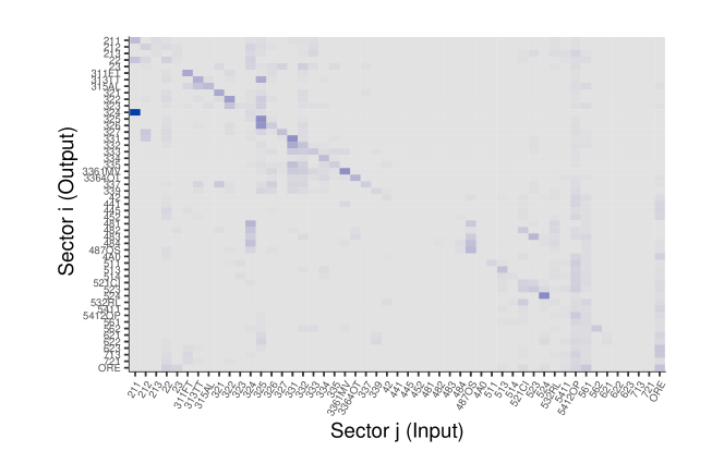
Figure A-1: Tabular Representation of the Input-Output Matrix
Notes: The figure shows the input-output matrix $A$, with darker shades of blue indicating stronger links $a_{ij}$.

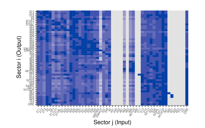
Figure A-2: Tabular Representation of Shortest Paths
Notes: The figure shows the matrix of shortest paths or distances from a sector $i$ to any other sector $j$, with darker shades of blue indicating longer distances.

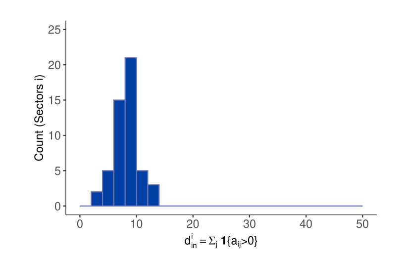
(a) In-Degrees

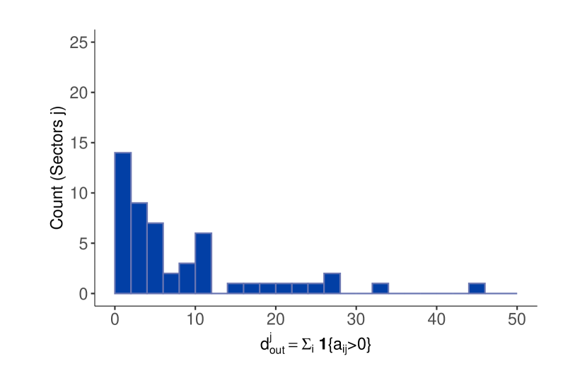
(b) Out-Degrees

Figure A-3: In-Degrees and Out-Degrees
Notes: The left panel plots in-degrees, equal to the number of non-zero entries by columns of $A$, which show the number of input-suppliers across sectors. The right panel plots out-degrees, equal to the number of non-zero entries by rows of $A$, which show the number of customers supplied across sectors.

Table A-1: Output Shares, Inflation Statistics and Network Statistics Across Sectors

Code	Name	Output [%]	Mean $\pi_{it}$	StdD $\pi_{it}$	Min $\pi_{it}$	Max $\pi_{it}$	$d^{in}_{i}$	$wd^{in}_{i}$	$d^{out}_{i}$	$wd^{out}_{i}$
211	Oil and gas extraction	$1.66$	$0.72$	$9.61$	$-32.68$	$34.30$	$10$	$0.30$	$3$	$0.97$
212	Mining, except oil and gas	$0.62$	$0.48$	$1.65$	$-5.11$	$9.81$	$11$	$0.30$	$6$	$0.34$
213	Support activities for mining	$0.46$	$0.23$	$1.29$	$-4.07$	$7.04$	$12$	$0.32$	$3$	$0.06$
22	Utilities	$2.61$	$0.62$	$8.19$	$-47.50$	$103.11$	$9$	$0.39$	$25$	$0.69$
23	Construction	$5.70$	$0.37$	$0.77$	$-1.61$	$5.84$	$12$	$0.41$	$5$	$0.13$
321	Wood products	$0.40$	$0.33$	$2.06$	$-10.02$	$10.04$	$7$	$0.37$	$5$	$0.42$
327	Nonmetallic mineral products	$0.52$	$0.29$	$0.42$	$-0.46$	$2.61$	$10$	$0.44$	$5$	$0.24$
331	Primary metals	$1.32$	$0.36$	$2.12$	$-7.15$	$9.33$	$10$	$0.56$	$11$	$1.07$
332	Fabricated metal products	$1.66$	$0.30$	$0.50$	$-0.85$	$2.61$	$9$	$0.47$	$24$	$0.92$
333	Machinery	$1.79$	$0.23$	$0.29$	$-0.17$	$2.05$	$11$	$0.47$	$11$	$0.37$
334	Computer and electronic products	$2.01$	$-0.01$	$0.25$	$-0.93$	$1.52$	$6$	$0.22$	$12$	$0.40$
335	Electrical equipment, appliances, and components	$0.61$	$0.28$	$0.49$	$-1.62$	$1.94$	$10$	$0.43$	$7$	$0.20$
3361MV	Motor vehicles, bodies and trailers, and parts	$2.44$	$0.11$	$0.61$	$-2.22$	$4.01$	$9$	$0.68$	$6$	$0.46$
3364OT	Other transportation equipment	$1.40$	$0.19$	$0.23$	$-0.57$	$1.07$	$12$	$0.43$	$3$	$0.25$
337	Furniture and related products	$0.32$	$0.25$	$0.35$	$-0.45$	$2.14$	$13$	$0.53$	$3$	$0.11$
339	Miscellaneous manufacturing	$0.90$	$0.15$	$0.27$	$-0.50$	$2.11$	$13$	$0.35$	$4$	$0.12$
311FT	Food and beverage and tobacco products	$4.34$	$0.28$	$0.89$	$-4.65$	$6.07$	$7$	$0.35$	$7$	$0.41$
313TT	Textile mills and textile product mills	$0.28$	$0.23$	$0.44$	$-0.76$	$1.70$	$9$	$0.53$	$9$	$0.46$
315AL	Apparel and leather and allied products	$0.13$	$0.12$	$0.25$	$-0.53$	$1.12$	$7$	$0.42$	$3$	$0.20$
322	Paper products	$0.95$	$0.26$	$0.52$	$-1.12$	$2.22$	$10$	$0.52$	$11$	$0.56$
323	Printing and related support activities	$0.47$	$0.19$	$0.44$	$-0.54$	$3.31$	$13$	$0.44$	$3$	$0.08$
324	Petroleum and coal products	$3.41$	$0.78$	$7.42$	$-33.28$	$22.76$	$3$	$0.76$	$21$	$1.00$
325	Chemical products	$4.01$	$0.33$	$0.70$	$-2.05$	$2.63$	$6$	$0.43$	$27$	$1.56$
326	Plastics and rubber products	$1.05$	$0.29$	$0.57$	$-1.14$	$2.54$	$7$	$0.52$	$16$	$0.46$
42	Wholesale trade	$6.73$	$0.32$	$0.88$	$-1.90$	$3.88$	$10$	$0.22$	$5$	$0.09$
441	Motor vehicle and parts dealers	$0.94$	$0.33$	$0.93$	$-2.72$	$5.20$	$6$	$0.19$	$0$	$0.00$
445	Food and beverage stores	$1.01$	$0.31$	$1.39$	$-2.99$	$4.06$	$7$	$0.20$	$0$	$0.00$
452	General merchandise stores	$1.01$	$0.23$	$3.29$	$-11.76$	$10.90$	$8$	$0.20$	$0$	$0.00$
4A0	Other retail	$3.43$	$0.25$	$1.61$	$-5.99$	$5.11$	$6$	$0.21$	$0$	$0.00$
481	Air transportation	$0.85$	$0.29$	$3.08$	$-9.89$	$13.25$	$5$	$0.36$	$0$	$0.00$
482	Rail transportation	$0.38$	$0.32$	$0.83$	$-2.72$	$2.77$	$10$	$0.40$	$1$	$0.01$
483	Water transportation	$0.27$	$0.32$	$1.42$	$-4.37$	$8.96$	$9$	$0.54$	$0$	$0.00$
484	Truck transportation	$1.41$	$0.30$	$0.80$	$-2.25$	$4.04$	$9$	$0.41$	$3$	$0.06$
487OS	Other transportation and support activities	$0.93$	$0.28$	$0.69$	$-1.40$	$4.31$	$9$	$0.33$	$6$	$0.51$
511	Publishing industries, except internet (includes software)	$1.62$	$0.08$	$0.47$	$-1.90$	$1.76$	$9$	$0.24$	$1$	$0.05$
513	Broadcasting and telecommunications	$3.70$	$0.05$	$0.45$	$-1.24$	$1.59$	$7$	$0.29$	$9$	$0.25$
514	Data processing, internet publishing, and other information services	$0.91$	$0.02$	$0.52$	$-2.23$	$2.07$	$9$	$0.24$	$3$	$0.05$
521CI	Federal Reserve banks, credit intermediation, and related activities	$3.88$	$0.07$	$2.59$	$-9.21$	$8.19$	$8$	$0.28$	$17$	$0.53$
523	Securities, commodity contracts, and investments	$2.54$	$0.35$	$1.63$	$-10.59$	$6.20$	$9$	$0.40$	$10$	$0.43$
524	Insurance carriers and related activities	$3.61$	$0.17$	$0.25$	$-0.14$	$1.71$	$3$	$0.39$	$11$	$0.55$
ORE	Other real estate	$4.51$	$0.15$	$0.40$	$-1.19$	$1.96$	$9$	$0.50$	$28$	$1.10$
532RL	Rental and leasing services and lessors of intangible assets	$1.46$	$0.18$	$1.82$	$-6.50$	$5.86$	$8$	$0.28$	$20$	$0.37$
5411	Legal services	$1.56$	$0.30$	$0.59$	$-0.72$	$3.27$	$7$	$0.17$	$12$	$0.17$
5412OP	Miscellaneous professional, scientific, and technical services	$5.74$	$0.16$	$0.51$	$-0.81$	$6.28$	$7$	$0.21$	$46$	$1.68$
561	Administrative and support services	$3.29$	$0.14$	$0.27$	$-0.69$	$1.17$	$7$	$0.15$	$34$	$0.94$
562	Waste management and remediation services	$0.46$	$0.24$	$0.53$	$-1.77$	$2.12$	$10$	$0.28$	$1$	$0.10$
621	Ambulatory health care services	$4.50$	$0.09$	$0.30$	$-1.10$	$2.80$	$7$	$0.21$	$2$	$0.03$
622	Hospitals	$3.57$	$0.21$	$0.34$	$-0.75$	$1.96$	$9$	$0.30$	$0$	$0.00$
623	Nursing and residential care facilities	$1.09$	$0.24$	$0.31$	$-0.83$	$1.52$	$8$	$0.25$	$0$	$0.00$
713	Amusements, gambling, and recreation industries	$0.60$	$0.11$	$0.65$	$-2.00$	$2.20$	$9$	$0.30$	$0$	$0.00$
721	Accommodation	$0.95$	$0.22$	$2.04$	$-8.85$	$9.23$	$8$	$0.21$	$0$	$0.00$
	Mean	$1.96$	$0.26$	$1.35$	$-5.03$	$7.14$	$8.61$	$0.36$	$8.61$	$0.36$
	StdD	$1.65$	$0.15$	$1.94$	$8.99$	$14.85$	$2.25$	$0.13$	$10.03$	$0.41$
	Min	$0.13$	$-0.01$	$0.23$	$-47.50$	$1.07$	$3.00$	$0.15$	$0.00$	$0.00$
	Max	$6.73$	$0.78$	$9.61$	$-0.14$	$103.11$	$13.00$	$0.76$	$46.00$	$1.68$

C.3 Estimation

Consistent with the restrictions implies by theory, for $\alpha$ I use a Uniform distribution on $[0,1]^{p-1}$ truncated to the region where $\sum_{l=1}^{p-1}\alpha_{l}\leq 1$:

$$\alpha_{1},...,\alpha_{p-1}\sim\prod_{l=1}^{p-1}\mathcal{U}(0,1)\;\mathbf{1}\left\{{\sum_{l=1}^{p-1}\alpha_{l}\leq 1}\right\}\;.$$

This leads to

$$p(\alpha_{1},...,\alpha_{p-1}) =p(\alpha_{1}|\alpha_{2},...,\alpha_{p-1})p(\alpha_{2}|\alpha_{3},...,\alpha_{p-1})...p(\alpha_{p-2}|\alpha_{p-1})p(\alpha_{p-1})$$

$$=\begin{cases}(p-1)!\quad&\text{if}\;\sum_{l=1}^{p-1}\alpha_{l}\leq 1\\ 0\quad&\text{otherwise}\end{cases}\;,$$

where for $l=1:p-2$,

$$p(\alpha_{l}|\alpha_{l+1},...,\alpha_{p-1})=\begin{cases}l\frac{\left({1-\sum_{m=l}^{p-1}\alpha_{m}}\right)^{l-1}}{\left({1-\sum_{m=l+1}^{p-1}\alpha_{m}}\right)^{l-1}}\quad&\text{if}\;\alpha_{l}\in\left[{0,1-\sum_{m=l+1}^{p-1}\alpha_{m}}\right]\\ 0\quad&\text{otherwise}\end{cases}\;,$$

and

$$p(\alpha_{p-1})=\begin{cases}(p-1)\left({1-\alpha_{p-1}}\right)^{p-2}\quad&\text{if}\;\alpha_{p-1}\in\left[{0,1}\right]\\ 0\quad&\text{otherwise}\end{cases}\;.$$

To draw from $p(\alpha_{1},...,\alpha_{p-1})$, I draw $\alpha_{p-1}$ from its marginal distribution and iteratively draw $\alpha_{p-2},...,\alpha_{1}$ from the conditionals. In each of these steps, efficient drawing from these non-standard distributions is implemented using the inverse-cdf method: to draw $y_{i}\sim f(y)$, I draw $x_{i}\sim\mathcal{U}(0,1)$ and find $y_{i}$ so that $\int_{-\infty}^{y_{i}}f(y)dy=x_{i}$. In the present case, this yields

$$\alpha_{l}|(\alpha_{l+1},...,\alpha_{p-1})=\left({1-\sum_{m=l+1}^{p-1}\alpha_{m}}\right)\left[{1-(1-x_{l})^{1/l}}\right]\;,\quad x_{l}\sim\mathcal{U}(0,1)\;,$$

for $l=1:{p-2}$, and $\alpha_{p-1}=1-(1-x_{p-1})^{1/(p-1)}$, $x_{p-1}\sim\mathcal{U}(0,1)$.

For the parameters in $\sigma$, only the lower bound of the prior distribution is determined by the domain restriction $\sigma_{i}>0$. The choice of the upper bound may appear non-trivial. If it is too low, it might restrict the posterior mode, if it is too large, posterior sampling will be inefficient. However, one can choose a lower bound low enough to ensure efficient computation and still allow the SMC sampler to go beyond the upper bound in the search for $\sigma_{i}$ associated with high likelihood values in case it is needed by not enforcing the upper bound as a domain restriction. In case the posterior contains draws that do not obey the boundary of the prior, the resulting marginal data density (MDD) will be wrong, but can be adjusted easily ex-post. Let $\bar{s}_{i}$ be the upper bound in the prior draws for $\sigma_{i}$, and take any $\bar{d}_{i}$. We have

$$p(Y) =\int p(Y|\theta)p(\theta)d\theta$$

$$=\int p(Y|\alpha,\sigma)p(\alpha)p(\sigma)d(\alpha,\sigma)$$

$$=(p-1)!\prod_{i=1}^{n}\frac{1}{\bar{s}_{i}}\int p(Y|\alpha,\sigma)d(\alpha,\sigma)\;,$$

so that the (estimated) $ln\;p(Y)$ returned by the SMC sampler,

$$ln\;p(Y)=ln\;(p-1)!-\sum_{i=1}^{n}ln\;\bar{s}_{i}+ln\;\int p(Y|\alpha,\sigma)d(\alpha,\sigma)\;,$$

can be adjusted to reflect an effective uniform prior for $\sigma_{i}$ with an upper bound different than the one used to initialize the sampler. For example, to go from $\mathcal{U}(0,\bar{s}_{i})$ to $\mathcal{U}(0,\bar{d}_{i})$, one adds $ln\;\bar{s}_{i}-ln\;\bar{d}_{i}$. To be able to use MDD as a model selection device, the prior for $\sigma$ and hence the effective prior upper bounds $\{\bar{d}_{i}\}_{i=1:n}$ should be the same for all different models indexed by $(q,p)$. I choose $\bar{s}_{i}=5\mathbb{V}[y_{it}]$ and abstract from the re-scaling of the MDD because its exact value is not of importance in the present analysis, only the relative values for different models.

In absence of more precise prior information (and in particular due to the wide priors for $\sigma_{i}$), the SMC algorithm would take a long time to converge if the proposal distribution is taken to be the prior (likelihood tempering). To ameliorate this issue, I use the model tempering variant of the SMC from Mlikota and Schorfheide (2022) and implement a mock model to construct a proposal distribution that tilts the prior draws for $\sigma$ towards values that are more compatible with high likelihood values conditional on the prior draws for $\alpha$. To do so, I obtain a consistent estimator for $\sigma|\alpha$ using the method of moments applied to the variance of the high-frequency process $\tilde{y}_{\tau}$. We know that $\mathbb{V}[y_{t}]=\mathbb{V}[\tilde{y}_{tq}]$. The latter can be computed as a function of $\Sigma$:

$$\mathbb{V}[\tilde{y}_{\tau}]=\Phi_{1}\mathbb{V}[\tilde{y}_{\tau}]\Phi_{1}^{\prime}+...+\Phi_{p}\mathbb{V}[\tilde{y}_{\tau}]\Phi_{p}^{\prime}+\Sigma\;,$$

which in turn implies

$$vec(\mathbb{V}[\tilde{y}_{\tau}]) =\left({\sum_{l=1}^{p}\Phi_{l}\otimes\Phi_{l}}\right)vec(\mathbb{V}[\tilde{y}_{\tau}])+vec(\Sigma)$$

$$=\left({\sum_{l=1}^{p}\alpha_{l}^{2}}\right)\left({A\otimes A}\right)vec(\mathbb{V}[\tilde{y}_{\tau}])+vec(\Sigma)\;.$$

Overall, we get

$$vec(\hat{\Sigma}_{MM}|\alpha)=\left[{I-\left({\sum_{l=1}^{p}\alpha_{l}^{2}}\right)\left({A\otimes A}\right)}\right]vec(\hat{\mathbb{V}}_{MM}[\tilde{y}_{\tau}])\;,\quad\hat{\mathbb{V}}_{MM}[\tilde{y}_{\tau}]=\hat{\mathbb{V}}_{MM}[y_{t}]=\frac{1}{T}\sum_{t=1}^{T}y_{t}y_{t}^{\prime}\;.$$

I then construct the likelihood for the mock model as the density of independent Inverse Gamma distributions for $\sigma_{i}$ with a mode at $\hat{\sigma}_{i,MM}|\alpha=(\hat{\Sigma}_{MM}|\alpha)_{ii}$. This means that the proposal distribution is the product of the prior for $\alpha$ and Inverse Gamma distributions for $\sigma_{i}|\alpha$.

I also use the adaptive tempering method proposed by Cai et al. (2021), which ensures a precise estimation of the posterior in the present case in which the distance between the proposal and posterior distributions is difficult to assess. Finally, to implement the algorithm under the presence of the tight domain restrictions for $\alpha$, I consider a transformation of the parameters in the mutation step of the SMC algorithm. Define the function $g$ s.t. $\check{\theta}=g^{-1}(\theta)$ is generated by taking logs of $\sigma_{i}$ and computing $\gamma_{l}=ln\;\alpha_{l}/\alpha_{p}$ for $\alpha_{1},...,\alpha_{p-1}$. Note that both are one-to-one mappings and ensure that the transformed parameters can fall everywhere on the real line. As a result, no draws in the mutation step are rejected because of domain violations. I use a Random Walk Metropolis Hastings (RWMH) algorithm in the mutation step. Even though the proposal density for the transformed draws is symmetric, for the original parameters it is not. The mutation step needs to be adjusted to reflect this. Overall, the mutation of particle $i$ in iteration $n$ of the SMC algorithm is performed as follows:

Algorithm 1 (Particle Mutation in SMC Algorithm).

1. Given particle $\theta^{i}_{n-1}$, set $\theta^{i,0}_{n}=\theta^{i}_{n-1}$.

2. For $m=1:N_{MH}$:

   • Compute $\check{\theta}^{i,m-1}_{n}=g^{-1}(\theta^{i,m-1}_{n})$ and draw

     $$\check{v}|\theta^{i,m-1}_{n}\sim\check{q}(\check{v}|\theta^{i,m-1}_{n})=N(\check{\theta}^{i,m-1}_{n},c_{n}^{2}\Sigma_{n})=N(g^{-1}(\theta^{i,m-1}_{n}),c_{n}^{2}\Sigma_{n})\;.$$

   • Set

     $$\theta^{i,m}_{n}=\begin{cases}v=g(\check{v})\;\quad&\text{w.p.}\quad\alpha(v|\theta^{i,m-1}_{n})\\ \theta^{i,m-1}_{n}\;\quad&\text{otherwise}\end{cases}\;,$$

     where

     $$\alpha(v|\theta^{i,m-1}_{n}) =min\;\left\{{1,\frac{p(Y|v)p(v)/q(v|\theta^{i,m-1}_{n})}{p(Y|\theta^{i,m-1}_{n})p(\theta^{i,m-1}_{n})/q(\theta^{i,m-1}_{n}|v)}}\right\}\;.$$

     The densities $q(v|\theta^{i,m-1}_{n})$ and $q(\theta^{i,m-1}_{n}|v)$ are obtained using analogous density transformations starting from $q(\check{v}|\theta^{i,m-1}_{n})$ and $q(\check{\theta}^{i,m-1}_{n}|v)$, respectively;

     $$q(v|\theta^{i,m-1}_{n})=\check{q}(g^{-1}(v)|\theta^{i,m-1}_{n})|J(v)|\;,$$

     where the Jacobian matrix $J(\theta)$ is block diagonal with

     $$J_{11}(\theta)=\begin{bmatrix}\alpha_{1}^{-1}&&0\\ &\ddots&\\ 0&&\alpha^{-1}_{p-1}\end{bmatrix}+\alpha_{p}^{-1}\iota\iota^{\prime}\;,\quad J_{22}(\theta)=\begin{bmatrix}\sigma_{1}^{-1}&&0\\ &\ddots&\\ 0&&\sigma_{N}^{-1}\end{bmatrix}\;.$$

3. Set $\theta^{i}_{n}=\theta^{i,N_{MH}}_{n}$.

Note that because $\check{q}(g^{-1}(v)|\theta^{i,m-1}_{n})=\check{q}(g^{-1}(\theta^{i,m-1}_{n})|v)$ is symmetric, we obtain

$$\alpha(v|\theta^{i,m-1}_{n})=min\;\left\{{1,\frac{p(Y|v)p(v)}{p(Y|\theta^{i,m-1}_{n})p(\theta^{i,m-1}_{n})}\frac{|J(\theta^{i,m-1}_{n})|}{|J(v)|}}\right\}\;,$$

and one can show that

$$ln\;\frac{|J(\theta^{i,m-1}_{n})|}{|J(v)|}=\sum_{j=1}^{N}\left[{ln\;\sigma_{j}-ln\;\sigma_{j,n}^{i,m-1}}\right]+ln\;|J_{11}(\theta^{i,m-1}_{n})|-ln\;|J_{11}(v)|\;.$$

C.4 Results

Table A-2: Model Selection

Log MDD
		$p$
		$1q$	$2q$	$3q$	$4q$	$5q$	$6q$
	1/3			19079			19044
	1/2		19384		18768		18690
$q$	1	20153	20056	19675	19879	18899	20218
	2	17546	19570	19248	20142	18662	19636
	4	18517	19808	19754	19655	18904	19301
BIC
		$p$
		$1q$	$2q$	$3q$	$4q$	$5q$	$6q$
	1/3			-38568			-38487
	1/2		-38849		-38194		-38089
$q$	1	-40964	-40799	-39650	-39944	-38060	-41060
	2	-36597	-39556	-39073	-40832	-37206	-39420
	4	-38096	-39883	-39648	-39274	-37806	-38659
AIC
		$p$
		$1q$	$2q$	$3q$	$4q$	$5q$	$6q$
	1/3			-38939			-38865
	1/2		-39220		-38572		-38474
$q$	1	-41335	-41177	-40036	-40336	-38460	-41467
	2	-36975	-39948	-39480	-41253	-37640	-39868
	4	-38488	-40304	-40098	-39753	-38313	-39194
Notes: The values for $q$ (from top to bottom) refer to quarterly, bi-monthly, monthly, bi-weekly and weekly network interactions, respectively, while $p=mq$ implies that the last $m$ months matter for dynamics.

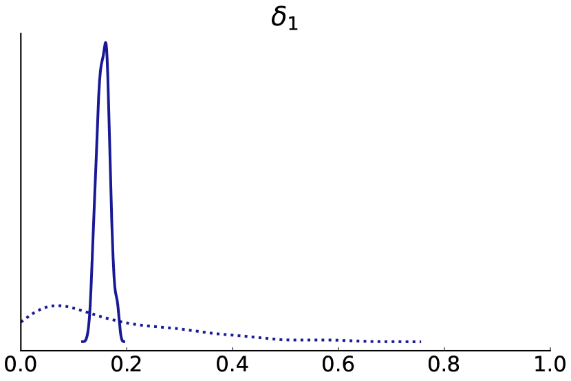
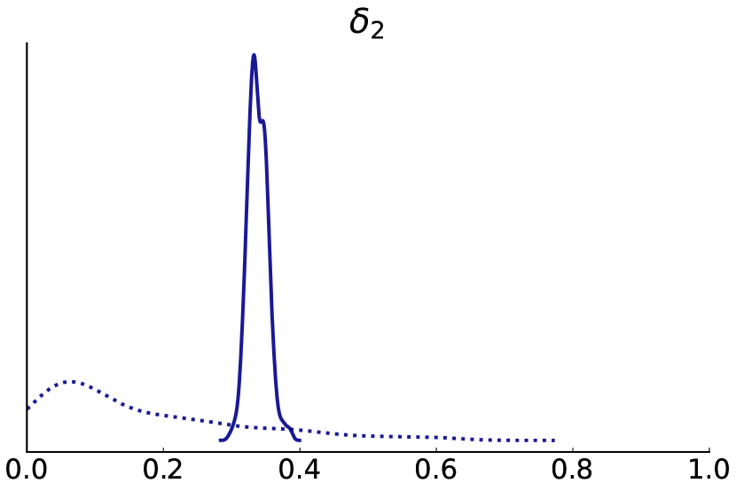
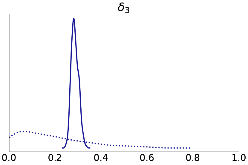
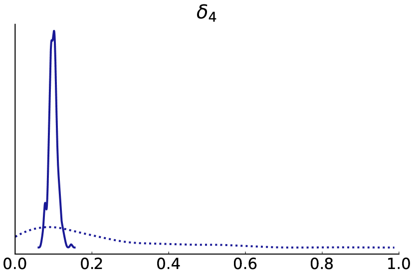
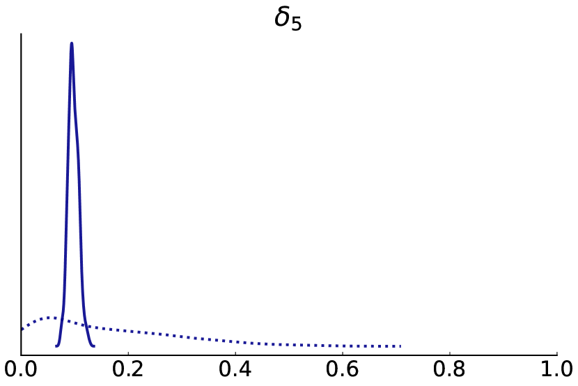
Figure A-4: Marginal Priors and Posteriors For $\alpha$
Notes: The solid line shows the posterior, the dotted line the prior.

Appendix D Forecasting Global Industrial Production Growth

D.1 NVAR($p,1$) & Factor Model: Equivalence Result

For expositional simplicity, the equivalence result is shown for an NVAR($2,1$). The extension to general $p$ is straightforward. The NVAR($2,1$) can be written as

$$y_{t}=A[\alpha_{1}y_{t-1}+\alpha_{2}y_{t-2}]+u_{t}\;.$$

Let $r$ denote the rank of $A$. We can find $n\times r$ and $r\times n$ matrices $B$ and $C$, both of full rank, such that $A=BC$. In turn, the NVAR($2,1$) can be represented as a factor model with $r$ factors:

$$y_{t}=BC[\alpha_{1}y_{t-1}+\alpha_{2}y_{t-2}]+u_{t}=\Lambda f_{t}+u_{t}\;.$$

The $n\times r$ matrix of loadings $\Lambda$ is given by $B$, while factor $k$ is given by $f_{kt}=\alpha_{1}C_{k\cdot}y_{t-1}+\alpha_{2}C_{k\cdot}y_{t-2}$, where $C_{k\cdot}$ denotes the $k$th row of $C$. Note that this factor representation is not unique, as an observationally equivalent process is obtained by writing $A=BC=BQQ^{-1}C=\tilde{B}\tilde{C}$ for any $r\times r$ full-rank matrix $Q$.

Conversely, let $y_{t}$ permit a factor structure, with $r$ factors evolving dynamically according to a VAR($2$):

$$y_{t}=\Lambda f_{t}+\xi_{t}\;,\quad f_{t}=\Phi_{1}f_{t-1}+\Phi_{2}f_{t-2}+\eta_{t}\;.$$

Using an argument similar to the one in Cesa-Bianchi and Ferrero (2021), take $r$ distinct vectors of weights $w^{k}=(w_{1}^{k},...,w_{n}^{k})$, $k=1:r$, and consider weighted averages of $\{y_{it}\}_{i=1}^{n}$ of the form

$$\sum_{i=1}^{n}w_{i}^{k}y_{it}=\sum_{i=1}^{n}w_{i}^{k}\Lambda_{i\cdot}f_{t}+\sum_{i=1}^{n}w^{k}_{i}\xi_{it}\;.$$

For $n$ large enough, $\bar{\xi}^{k}_{t}\equiv\sum_{i=1}^{n}w^{k}_{i}\xi_{it}\sim O_{p}(n^{-1/2})$ is negligible and we can write

$$Wy_{t}=W\Lambda f_{t}\;,$$

where the $r\times n$ matrix $W$ stacks $w^{k\prime}$ along rows. In turn, we can solve for $f_{t}=(W\Lambda)^{-1}Wy_{t}$. As this equation holds for all $t$, we can re-write the process for $y_{t}$ as

$$y_{t} =\Lambda\left({\Phi_{1}f_{t-1}+\Phi_{2}f_{t-2}+\eta_{t}}\right)+\xi_{t}$$

$$=\Lambda\Phi_{1}(W\Lambda)^{-1}Wy_{t-1}+\Lambda\Phi_{2}(W\Lambda)^{-1}Wy_{t-2}+u_{t}\;,$$

with $u_{t}=\Lambda\eta_{t}+\xi_{t}$. If the dynamic evolution of the $r$ factors is restricted to an NVAR($2,1$), then $\Phi_{1}=\phi_{1}\Phi$ and $\Phi_{2}=\phi_{2}\Phi$ for some $\phi_{1},\phi_{2},\Phi$, and the above equation simplifies to

$$y_{t}=\Lambda\Phi(W\Lambda)^{-1}W[\phi_{1}y_{t-1}+\phi_{2}y_{t-2}]+u_{t}\;.$$

This equation implies that $y_{t}$ follows an NVAR($2,1$) with adjacency matrix $A=\Lambda\Phi(W\Lambda)^{-1}W$. $A$ has rank $r$ and can be written as $A=BC$ with $B=\Lambda Q$, $C=Q^{-1}\Phi(W\Lambda)^{-1}W$ for any $r\times r$ orthogonal matrix $Q$. Note that we can re-scale $A$ and $(\phi_{1},\phi_{2})$ in case an element in $A$ exceeds unity (see Section 3.2).

D.2 Application Details

Table A-3: Descriptive Data Statistics and Estimated Outdegrees

Code	Name	Mean $y_{it}$	StdD $y_{it}$	Min $y_{it}$	Max $y_{it}$	$\hat{wd}^{out}_{i}$
AUT	Austria	$-0.14$	$7.11$	$-25.92$	$32.05$	$0.00$
BGD	Bangladesh	$2.09$	$8.51$	$-33.49$	$65.66$	$0.90$
BEL	Belgium	$0.62$	$7.53$	$-22.55$	$36.17$	$0.00$
BRA	Brazil	$-0.74$	$7.09$	$-29.14$	$33.29$	$1.07$
CAN	Canada	$0.07$	$5.58$	$-20.86$	$15.40$	$1.69$
CHL	Chile	$0.12$	$4.40$	$-13.09$	$12.39$	$0.72$
COL	Colombia	$0.45$	$7.88$	$-36.73$	$58.73$	$2.94$
CRI	Costa Rica	$-0.60$	$3.93$	$-14.67$	$12.74$	$0.19$
CYP	Cyprus	$-0.35$	$8.40$	$-37.58$	$58.53$	$0.95$
CZE	Czech Republic	$0.58$	$8.37$	$-37.33$	$51.70$	$0.04$
DEU	Germany	$-0.21$	$7.84$	$-31.27$	$35.07$	$0.00$
DNK	Denmark	$0.19$	$6.77$	$-21.50$	$22.43$	$0.09$
EST	Estonia	$-0.09$	$10.79$	$-40.17$	$31.80$	$0.57$
ESP	Spain	$-1.24$	$7.85$	$-35.60$	$51.00$	$0.00$
FIN	Finland	$-1.30$	$6.71$	$-27.86$	$21.42$	$0.12$
FRA	France	$-0.71$	$6.50$	$-35.64$	$43.58$	$0.00$
GBR	United Kingdom	$-0.78$	$5.81$	$-26.57$	$28.56$	$1.02$
GRC	Greece	$-0.18$	$8.52$	$-25.33$	$21.84$	$0.52$
HRV	Croatia	$-0.17$	$5.42$	$-16.18$	$15.68$	$0.24$
HUN	Hungary	$1.11$	$9.20$	$-39.83$	$56.31$	$0.06$
IRL	Ireland	$-1.52$	$16.10$	$-38.83$	$59.64$	$1.41$
ISR	Israel	$0.08$	$8.12$	$-22.43$	$31.42$	$0.15$
IND	India	$-2.13$	$11.35$	$-58.94$	$127.82$	$0.16$
ISL	Iceland	$0.29$	$13.65$	$-25.78$	$50.08$	$1.11$
ITA	Italy	$-0.56$	$9.52$	$-29.31$	$78.25$	$0.00$
JOR	Jordan	$-0.14$	$7.86$	$-25.26$	$26.30$	$1.90$
JPN	Japan	$-1.28$	$8.40$	$-37.18$	$26.70$	$1.16$
KOR	Korea, Republic of	$-3.03$	$7.10$	$-32.63$	$31.36$	$2.77$
LTU	Lithuania	$0.48$	$9.28$	$-31.29$	$33.41$	$0.57$
LUX	Luxembourg	$-1.01$	$8.64$	$-34.17$	$42.01$	$0.47$
LVA	Latvia	$-0.10$	$7.95$	$-31.12$	$20.58$	$0.70$
MKD	North Macedonia, Republic of	$1.11$	$9.34$	$-22.59$	$32.46$	$0.46$
MEX	Mexico	$-1.01$	$5.63$	$-31.73$	$34.86$	$0.19$
MYS	Malaysia	$-1.54$	$5.45$	$-22.03$	$13.90$	$1.44$
NLD	Netherlands	$-0.36$	$5.78$	$-21.61$	$20.80$	$0.63$
NOR	Norway	$-2.38$	$5.32$	$-15.40$	$10.80$	$0.61$
POL	Poland	$1.24$	$6.59$	$-29.50$	$40.54$	$2.04$
PRT	Portugal	$-1.99$	$6.04$	$-30.68$	$36.22$	$2.04$
RUS	Russian Federation	$1.74$	$4.95$	$-18.98$	$11.01$	$3.46$
SWE	Sweden	$-1.00$	$6.49$	$-24.47$	$20.95$	$2.62$
SVN	Slovenia	$0.10$	$7.06$	$-27.74$	$32.12$	$2.90$
SVK	Slovakia	$1.97$	$10.31$	$-45.26$	$65.41$	$1.30$
TUR	Turkey	$0.58$	$9.19$	$-35.66$	$59.56$	$2.24$
USA	United States	$-1.24$	$4.65$	$-18.84$	$14.73$	$3.94$

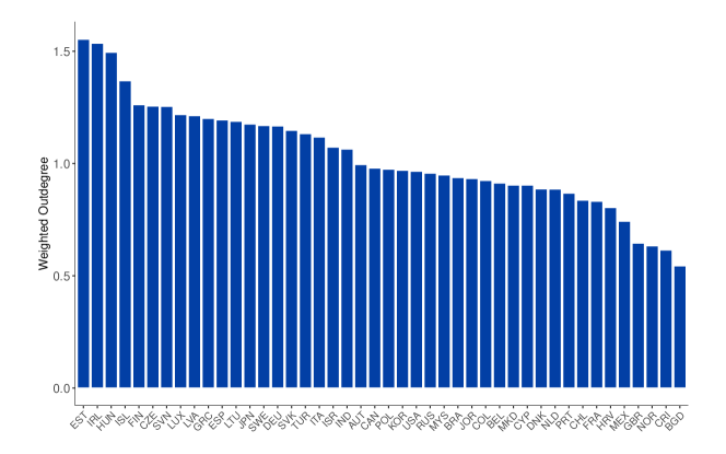
Figure A-5: Weighted Indegrees in the Estimated Network
Notes: The plot depicts the weighted indegrees in the estimated network as relevant for monthly industrial production dynamics across countries.

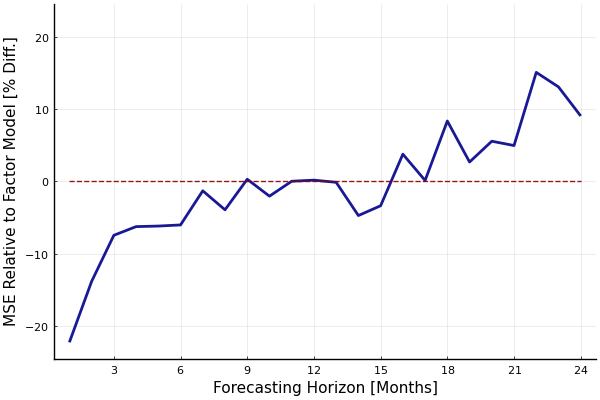
(a) $p=1$

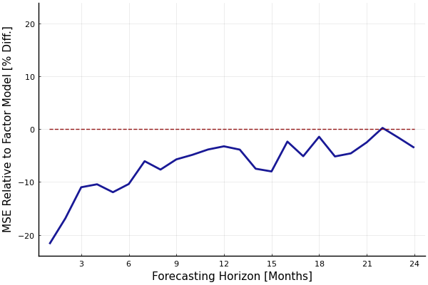
(b) $p=2$

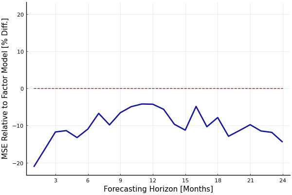
(c) $p=3$

(d) $p=4$

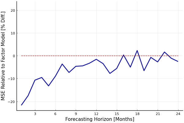
(e) $p=5$

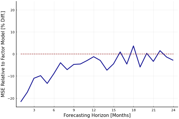
(f) $p=6$

Figure A-6: Out-of-Sample Forecasting Performance: NVAR($p,1$) vs. Factor Model
Notes: The plot depicts the percentage difference between the out-of-sample Mean Squared Errors generated by the NVAR($p,1$) to those generated by the Principal Components Factor Model for different choices of $p$.

References

- Acemoglu et al. (2016) Acemoglu, D., U. Akcigit, and W. Kerr (2016): “Networks and the macroeconomy: an empirical exploration,” NBER Macroeconomics Annual, 30, 273–335.
- Acemoglu et al. (2012) Acemoglu, D., V. M. Carvalho, A. Ozdaglar, and A. Tahbaz-Salehi (2012): “The Network Origins of Aggregate Fluctuations,” Econometrica, 80, 1977–2016.
- Bai and Ng (2002) Bai, J. and S. Ng (2002): “Determining The Number Of Factors In Approximate Factor Models,” Econometrica, 70, 191–221.
- Barigozzi and Brownlees (2018) Barigozzi, M. and C. Brownlees (2018): “NETS: Network Estimation for Time Series,” Journal of Applied Econometrics, 34, 347–364.
- Barigozzi et al. (2022) Barigozzi, M., G. Cavaliere, and G. Moramarco (2022): “Factor Network Autoregressions,” Manuscript, University of Bologna.
- Berman and Plemmons (1979) Berman, A. and R. J. Plemmons (1979): Nonnegative Matrices in the Mathematical Sciences.
- Boivin and Ng (2006) Boivin, J. and S. Ng (2006): “Are more data always better for factor analysis?” Journal of Econometrics, 132, 169–194.
- Bouakez et al. (2014) Bouakez, H., E. Cardia, and F. Ruge-Murcia (2014): “Sectoral price rigidity and aggregate dynamics,” European Economic Review, 65, 1–22.
- Bramoullé et al. (2009) Bramoullé, Y., H. Djebbari, and B. Fortin (2009): “Identification of peer effects through social networks,” Journal of Econometrics, 150, 41–55.
- Bramoullé et al. (2016) Bramoullé, Y., A. Galeotti, and B. W. Rogers (2016): The Oxford Handbook of the Economics of Networks.
- Bykhovskaya (2021) Bykhovskaya, A. (2021): “Time Series Approach to the Evolution of Networks: Prediction and Estimation,” Journal of Business & Economic Statistics, forthcoming.
- Cai et al. (2021) Cai, M., M. D. Negro, E. Herbst, E. Matlin, R. Sarfati, and F. Schorfheide (2021): “Online estimation of DSGE models,” Econometrics Journal, 24, C33–C58.
- Camehl (2022) Camehl, A. (2022): “Penalized estimation of panel vector autoregressive models: A panel LASSO approach,” International Journal of Forecasting, forthcoming.
- Caporin et al. (2023) Caporin, M., D. Erdemlioglu, and S. Nasini (2023): “Estimating Financial Networks by Realized Interdependencies: A Restricted Vector Autoregressive Approach,” Manuscript, University of Padova.
- Carriero et al. (2011) Carriero, A., G. Kapetanios, and M. Marcellino (2011): “Forecasting large datasets with Bayesian reduced rank multivariate models,” Journal of Applied Econometrics, 26, 735–761.
- Carter and Kohn (1994) Carter, C. K. and R. Kohn (1994): “On Gibbs Sampling for State Space Models,” Biometrika, 81, 541–553.
- Carvalho (2014) Carvalho, V. M. (2014): “From Micro to Macro via Production Networks,” Journal of Economic Perspectives, 28, 23–48.
- Carvalho and Reischer (2021) Carvalho, V. M. and M. Reischer (2021): “Pathways to Persistence,” Manuscript, University of Cambridge.
- Carvalho and Tahbaz-Salehi (2019) Carvalho, V. M. and A. Tahbaz-Salehi (2019): “Production Networks: A Primer,” Annual Review of Economics, 11, 635–663.
- Cesa-Bianchi and Ferrero (2021) Cesa-Bianchi, A. and A. Ferrero (2021): “The Transmission of Keynesian Supply Shocks,” Manuscript, Bank of England.
- Dahlhaus et al. (2021) Dahlhaus, T., J. Schaumburg, and T. Sekhposyan (2021): “Networking the yield curve: implications for monetary policy,” ECB Working Paper Series.
- Diebold and Yilmaz (2009) Diebold, F. X. and K. Yilmaz (2009): “Measuring Financial Asset Return and Volatility Spillovers, With Application to Global Equity Markets,” The Economic Journal, 119, 158–171.
- Diebold and Yilmaz (2014) ——— (2014): “On the network topology of variance decompositions: Measuring the connectedness of financial firms,” Journal of Econometrics, 182, 119–134.
- Dufour and Renault (1998) Dufour, J.-M. and E. Renault (1998): “Short Run and Long Run Causality in Time Series: Theory,” Econometrica, 66, 1099–1125.
- Elliott et al. (2014) Elliott, M., B. Golub, and M. O. Jackson (2014): “Financial networks and contagion,” American Economic Review, 104, 3115–3153.
- Fan et al. (2023) Fan, J., S. Hong, and F. Parro (2023): “Learning and Expectations in Dynamic Spatial Economies,” NBER Working Paper Series, No. 31504.
- Fan et al. (2021) Fan, J., R. Masini, and M. C. Medeiros (2021): “Bridging factor and sparse models,” Manuscript, Princeton University.
- Foerster et al. (2011) Foerster, A. T., P.-D. G. Sarte, and M. W. Watson (2011): “Sectoral versus Aggregate Shocks: A Structural Factor Analysis of Industrial Production,” Journal of Political Economy, 119.
- Freyaldenhoven (2022) Freyaldenhoven, S. (2022): “Identification Through Sparsity in Factor Models: the L1-rotation criterion,” Manuscript, Federal Reserve Bank of Philadelphia.
- Geweke (1984) Geweke, J. (1984): “Inference and Causality in Economic Time Series Models,” Handbook of Econometrics, 11, 1101–1144.
- Giannone et al. (2015) Giannone, D., M. Lenza, and G. E. Primiceri (2015): “Prior selection for vector autoregressions,” Review of Economics and Statistics, 97, 436–451.
- Giovanni et al. (2018) Giovanni, J. D., A. A. Levchenko, and I. Mejean (2018): “The micro origins of international business-cycle comovement,” American Economic Review, 108, 82–108.
- Giroud and Mueller (2019) Giroud, X. and H. M. Mueller (2019): “Firms’ internal networks and local economic shocks,” American Economic Review, 109, 3617–3649.
- Golub and Jackson (2010) Golub, B. and M. O. Jackson (2010): “Naïve Learning in Social Networks and the Wisdom of Crowds,” American Economic Journal: Microeconomics, 2, 112–149.
- Graham (2020) Graham, B. S. (2020): “Network data,” Handbook of Econometrics.
- Hipp (2020) Hipp, R. (2020): “On Causal Networks of Financial Firms: Structural Identification via Non-Parametric Heteroskedasticity,” Staff Working Paper, Bank of Canada.
- Horvath (2000) Horvath, M. (2000): “Sectoral Shocks and Aggregate Fluctuations,” Journal of Monetary Economics, 45, 69–106.
- Hsu et al. (2008) Hsu, N. J., H. L. Hung, and Y. M. Chang (2008): “Subset selection for vector autoregressive processes using Lasso,” Computational Statistics and Data Analysis, 52, 3645–3657.
- Knight et al. (2016) Knight, M. I., M. A. Nunes, and G. P. Nason (2016): “Modelling, Detrending and Decorrelation of Network Time Series,” Manuscript, University of Bristol.
- Lee (2007) Lee, L. F. (2007): “Identification and estimation of econometric models with group interactions, contextual factors and fixed effects,” Journal of Econometrics, 140, 333–374.
- Long and Plosser (1983) Long, J. B. J. and C. I. Plosser (1983): “Real Business Cycles,” Journal of Political Economy, 93, 36–69.
- Manski (1993) Manski, C. F. (1993): “Identification of Endogenous Social Effects: The Reflection Problem,” Review of Economic Studies, 60, 531–542.
- Mehl et al. (2023) Mehl, A., M. Mlikota, and I. V. Robays (2023): “How Does a Dominant Currency Replace Another? Evidence from European Trade,” Manuscript, European Central Bank.
- Mlikota and Schorfheide (2022) Mlikota, M. and F. Schorfheide (2022): “Sequential Monte Carlo With Model Tempering,” Manuscript, University of Pennsylvania.
- Onatski (2012) Onatski, A. (2012): “Asymptotics of the principal components estimator of large factor models with weakly influential factors,” Journal of Econometrics, 168, 244–258.
- Palm and Nijman (1984) Palm, F. C. and T. E. Nijman (1984): “Missing Observations in the Dynamic Regression Model,” Econometrica, 52, 1415–1435.
- Pesaran et al. (2004) Pesaran, M. H., T. Schuermann, and S. M. Weiner (2004): “Modeling Regional Interdependences Using a Global Error-Correcting Macroeconometric Model,” Journal of Business and Economic Statistics, 22, 129–162.
- Phillips (1973) Phillips, P. C. B. (1973): “The Problem of Identification in Finite Parameter Continuous Time Models,” Journal of Econometrics, 1, 351–362.
- Stock and Watson (2002) Stock, J. H. and M. W. Watson (2002): “Forecasting using principal components from a large number of predictors,” Journal of the American Statistical Association, 97, 1167–1179.
- Tibshirani (1996) Tibshirani, R. (1996): “Regression Shrinkage and Selection Via the Lasso,” Journal of the Royal Statistical Society: Series B (Methodological), 58, 267–288.
- Velu et al. (1986) Velu, R. P., G. C. Reinsel, and D. W. Wichern (1986): “Reduced Rank Models for Multiple Time Series,” Biometrika, 73, 105–118.
- Yang and Lee (2019) Yang, K. and L. F. Lee (2019): “Identification and estimation of spatial dynamic panel simultaneous equations models,” Regional Science and Urban Economics, 76, 32–46.
- Zhu et al. (2017) Zhu, X., R. Pan, G. Li, Y. Liu, and H. Wang (2017): “Network vector autoregression,” Annals of Statistics, 45, 1096–1123.
- Zou et al. (2007) Zou, H., T. Hastie, and R. Tibshirani (2007): “On the ”degrees of freedom” of the lasso,” Annals of Statistics, 35, 2173–2192.