Inference of cosmological models with principal component analysis

Abstract

Determination of cosmological parameters is a major goal in cosmology at present. Availability of improved data sets necessitates development of novel statistical tools to interpret the inference from a cosmological model. In this paper, we combine the Principal Component Analysis (PCA) and Markov Chain Monte Carlo (MCMC) method to infer the parameters of cosmological models. We use the No U-Turn Sampler (NUTS) to run the MCMC chains in the model parameter space. After determining the observable by PCA, we replace the observational and the error part of the likelihood analysis with the PCA reconstructed observable and find out the most preferred model parameter set. After testing our methodology with simulated data, we apply the same to the observed data sets, the Hubble parameter data and Supernova Type Ia data. We assume a polynomial expansion as the parameterization of the dark energy equation of state. We show that this method is effective in constraining cosmological parameters from data, including sparse data sets.

organization=Indian Institue of Science Education and Research, addressline=Knowledge City, Manauli, Punjab, city=Mohali, postcode=140306, state=Punjab, country=India

1 Introduction

Observational evidence of the acceleration of the Universe marked the beginning of a new era in Cosmology. It is well established that the current expansion of the Universe is accelerating and an explanation for the current acceleration is by way of introducing Dark Energy(DE) term in the Einstein equation. Dark energy is described by its equation of state parameter (EoS) $w=-P^{\prime}/\rho^{\prime}$, where $\rho^{\prime}$ is the energy density and $P^{\prime}$ is its pressure contribution. It is still unknown whether dark energy is a cosmological constant (Carroll et al., 1992; Carroll, 2001; Turner and White, 1997; Padmanabhan, 2003) or a time-evolving entity (Peebles and Ratra, 2003; Copeland et al., 2006). The $\Lambda CDM$ (cosmological constant and cold dark matter) model corresponds to dark energy equation of state value $w=-1$, whereas in the case of time-evolving dark energy, the dark energy equation of state parameter varies with time and can assume different values of $w$ (Padmanabhan, 2003; Peebles and Ratra, 2003; Carroll et al., 1992; Weinberg, 1989; Coble et al., 1997; Caldwell et al., 1998; Sahni and Starobinsky, 2000; Ellis, 2003; Linder, 2008; Frieman et al., 2008; Albrecht et al., 2006; Stern et al., 2010; Arjona and Nesseris, 2020). Various models based on scalar, canonical and non-canonical fields have been proposed to overcome different problems of $\Lambda CDM$ model (Ratra and Peebles, 1988; Linder, 2006; Caldwell and Linder, 2005; Linder, 2008; Huterer and Peiris, 2007; Zlatev et al., 1999; Copeland et al., 1998; Padmanabhan, 2002; Singh et al., 2019; Bagla et al., 2003; Tsujikawa, 2013; Rajvanshi and Bagla, 2019; Chevallier and Polarski, 2001). The discrepancies in $H_{0}$ measurements and its implication in cosmological model selection is discussed in Banerjee et al. (2021); Lee et al. (2022). The last two decades have also marked the era of precision Cosmology, cosmological parameters are measured to high precision with the availability of new data-sets (Planck Collaboration et al., 2018; Chevallier and Polarski, 2001; Sangwan et al., 2018).

Maximum Likelihood Estimation analysis(MLE) is the most commonly used technique in cosmological parameter estimation(Singh et al., 2019; Jassal, 2009; Nesseris and Perivolaropoulos, 2004, 2005, 2007; Sangwan et al., 2018). The increasing availability of the observational data-set has tightened the constraints on the parameters of theoretical models (Chevallier and Polarski, 2001; Linder, 2003; Jassal et al., 2005; Gong and Wang, 2007; Mukherjee, 2016; Vagnozzi et al., 2018; Di Valentino et al., 2017; Bellomo et al., 2020; Bernal et al., 2020; Verde et al., 2013). Though it is crucial to determine the theory parameters, we have the observational data dependencies in the core of these methods, and new data sets reject or accept a particular model with quantified precision. Methods like the Principal Component Analysis (PCA) enable us to determine the the functional form of the observable a data-set in a model independent, non-parametric manner (Huterer and Starkman, 2003; Huterer and Cooray, 2005; Zheng and Li, 2017; Ishida and de Souza, 2011; Crittenden et al., 2009; Clarkson and Zunckel, 2010; Miranda and Dvorkin, 2018; Sharma et al., 2020; Hart and Chluba, 2019; Nesseris and García-Bellido, 2013; Nair and Jhingan, 2013; Hojjati et al., 2012; Hart and Chluba, 2022). PCA is a multivariate analysis and it gives the form of cosmological quantities as a function of redshift (Huterer and Starkman, 2003; Clarkson and Zunckel, 2010; Huterer and Cooray, 2005; Zheng and Li, 2017; Sharma et al., 2020). In our previous work Sharma et al. (2020) we combine PCA and Correlation Coefficient Calculation to give the analytical functional form of the observable quantity when observational data-sets are given as input. The method is efficient in fitting the observable, the caveat is that the cosmological parameters like the dark energy equation of state parameter cannot be directly determined. The problem is due to the non-linear dependency of the dark energy parameter to the observational quantity at hand, for instance, the Hubble parameter and the distance modulus. To circumvent this problem, we incorporate the Markov Chain Monte Carlo method to derive the equation of state parameters for dark energy and other cosmological parameters. The equation of state parameter is derived by searching for the model which best describes the functional form of the observable determined by the observational data. For the Monte Carlo method, we use the No U-Turn Sampler. We show that the constraints on the dark energy equation of state parameters are consistent with the constraints obtained from other methods.

This paper is structured as follows. In section 2, after a brief review of background cosmology, we describe the reconstruction algorithm along with the No U-turn sampling, followed by section 3, where we describe the results of our algorithm. In section 4, we conclude by summarising the main results of this paper.

2 Reconstruction

In this section, we first discuss the methodology of the Principal Component Analysis reconstruction (Sharma et al. (2020)) and the modification to the algorithm.

2.1 Reconstruction of the functional form of Hubble parameter and distance modulus in terms of redshift

For a spatially flat Universe, composed of dark energy and non-relativistic matter, the Hubble parameter is given by,

$$H(z)=H_{0}\left[\Omega_{m}(1+z)^{3}+\Omega_{DE}e^{3\int^{z}_{0}\frac{1+w(z^{\prime})}{1+z^{\prime}}dz^{\prime}}\right]^{1/2}.$$ (1)

The dark energy equation of state parameter $w(z)=P/\rho$ can be written as

$$w(z)=\sum_{i=1}^{m}\alpha_{i}\mathcal{F}(z)^{(i-1)},\hskip 14.22636pt\mathcal{F}(z)=\frac{z}{(1+z)}.$$ (2)

where $H_{0}$ denotes the present-day value of the Hubble parameter and $\Omega_{m}$, $\Omega_{DE}$ are the density parameters for matter and dark energy respectively. In eqn(2), $m=2$ corresponds to the Chevallier-Polarski-Linder(CPL) parameterization (Chevallier and Polarski, 2001; Linder, 2003) given by, $w(z)=w_{0}+w^{\prime}\frac{z}{1+z}$, $w_{0}$ and $w^{\prime}$ being the present day values of the equation state parameter and its derivative respectively. The equation gives the Taylor series expression of the dark energy equation of state parameter in terms of $(1-a)$, where $a$ is the scale factor.

From the functional form of the Hubble parameter, we can reconstruct the dark energy equation of state parameter $w(z)$. Differentiating eqn (1) we get,

$$w(z)=\frac{3h^{2}-2(1+z)hh^{\prime}}{3h_{0}^{2}(1+z)^{3}\Omega_{m}-3h^{2}},$$ (3)

where $h$ is the reduced Hubble parameter given by $H(z)=100h~{}kms^{-1}Mpc^{-1}$.

The luminosity distance $d_{L}(z)$ is given by,

$$d_{L}(z)=\frac{c}{H_{0}}(1+z)\int_{0}^{z}d_{H}(z^{\prime})dz^{\prime}$$ (4)

where $d_{H}$, from eq(1) is,

$$d_{H}(z)=\left(\Omega_{m}(1+z)^{3}+\Omega_{x}e^{{3\int_{0}^{z}\frac{(1+w(z^{\prime}))dz^{\prime}}{(1+z^{\prime})}}}\right)^{-1/2}$$ (5)

and is related to the distance modulus as

$$\mu(z)=5\log{\left(\frac{d_{L}}{1Mpc}\right)}+25$$ (6)

We use the same expression of eqn(2) for EoS to express $\mu(z)$.

Since $D(z)=(H_{0}/c)(1+z)^{-1}d_{L}(z)$, the equation of state parameter is given by

$$w(z)=\frac{2(1+z)D^{\prime\prime}+3D^{\prime}}{3D^{\prime 3}\Omega_{m}(1+z)^{3}-3D^{\prime}}$$ (7)

In our earlier work Sharma et al. (2020), we combined correlation coefficient calculation with PCA to quantitatively reconstruct the best fit cosmological model. We start by calculating the functional form of the reduced Hubble parameter $h(z)$ and distance modulus $\mu(z)$ directly from the data-set, using Principal Component Analysis (Sharma et al., 2020).

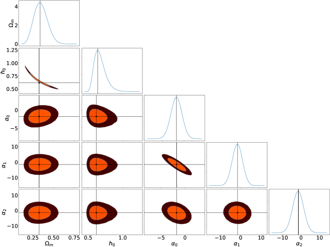
Figure 1: The plot show the $1\sigma$ and $2\sigma$ contours for all the parameters along with their marginal probability density plots for the case of simulated data-set.

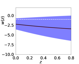
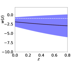
Figure 2: In this figure, we show the $68\%$ confident level range for the equation of state parameter $w(z)$. The figure on the left is for the simulated Hubble parameter data set, and the right one is for the real data set. The value of observational points $n_{d}$ and sample points $M_{s}$ are 600 and 800000, respectively. The black and red curves are the median and mean of the posterior density function. The cosmological constant model is consistent with the data and is denoted by the dashed line. The black and red solid lines represent the mean and median of the posterior density function. For both the plots these two lines overlap and this represents the best fit model.

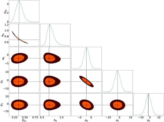
Figure 3: The plot show the $1\sigma$ and $2\sigma$ contours for all the parameters along with their marginal probability density plots for the case of real data-set (Zhang et al., 2014; Simon et al., 2005; Moresco et al., 2012; Ratsimbazafy et al., 2017; Moresco, 2015).

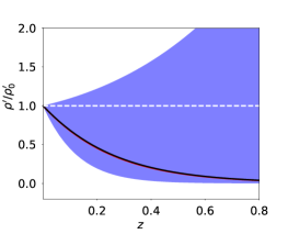
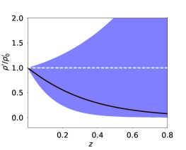
Figure 4: In this figure, we show the $68\%$ confident level range for the dark energy energy density evolution $\frac{\rho^{\prime}}{\rho^{\prime}_{0}}$. Here, $\rho^{\prime}$ and $\rho^{\prime}_{0}$ are the dark energy density at redshift $z$ and at present time respectively. Similar to the figure 2, the left figure is for the simulated Hubble parameter data set, and the right is for the real data set. The value of observational points $n_{d}$ and sample points $M_{s}$ are 600 and 800000, respectively. The black and red curves are the median and mean of the posterior density function. The cosmological constant model is consistent with the data and is denoted by the dashed white line. The black and red solid lines represent the mean and median of the posterior density function. For both the plots these two lines overlap and this represents the best fit model.

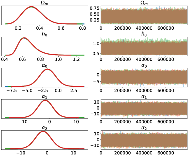
Figure 5: The column on the left consists of a smoothed histogram, using kernel density estimation of the marginal posteriors of each stochastic random variable. From top to bottom, the random variables are density parameters for matter $\Omega_{m}$, reduced Hubble constant $h_{0}$, and the parameters of the equation of state of dark energy $\alpha_{i}$, where we plot only the first three. The right column contains the samples of the Markov chain plotted in sequential order. There are four MCMC chains that are plotted in different colors. These pots are created with $(n_{d},M_{s})=(600,800000)$ and all are for simulated Hubble parameter data-set. We use the same values of $n_{d}$ and $M_{s}$ in subsequent plots.

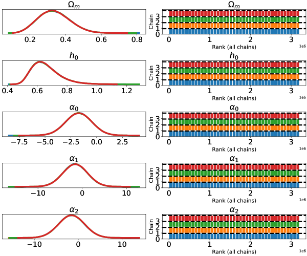
Figure 6: Smoothed histogram using kernel density estimation of the marginal posteriors of each stochastic random variable. From the top to bottom, the random variables are density parameters for matter $\Omega_{m}$, reduced Hubble constant $h_{0}$, and the parameters of the equation of state of dark energy $\alpha_{i}$. The right column shows the number of successful draws from the parameter space, which depends upon the sample size chosen as well as the prior theory. The four MCMC chains are plotted in different colors and all are independent of each other.

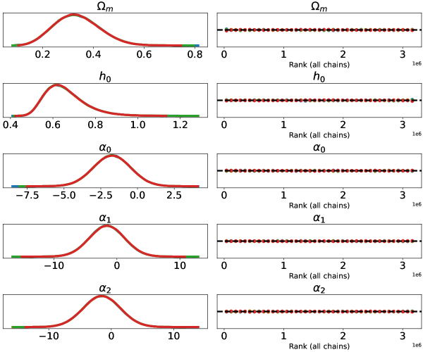
Figure 7: In this figure, the left column consists of a smoothed histogram, using kernel density estimation of the marginal posteriors of each stochastic random variable. The right-hand column gives the auto-correlation for all the random variables for all four independent chains, which are depicted with vertical lines.

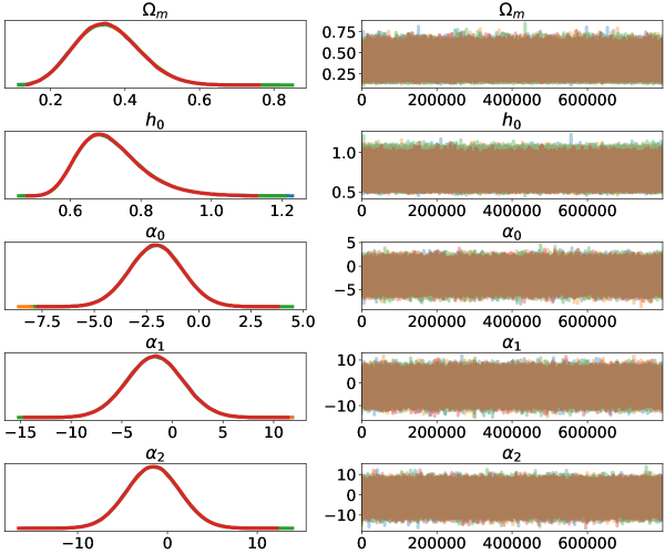
Figure 8: In this figure, the left column consists of a smoothed histogram, using kernel density estimation of the marginal posteriors of each stochastic random variable. The parameters are same as those in fig(5). The right column contains the samples of the Markov chain plotted in sequential order. These plots are also created with $(n_{d},M_{s})=(600,800000)$ and all the plots are for observed Hubble parameter data-set.

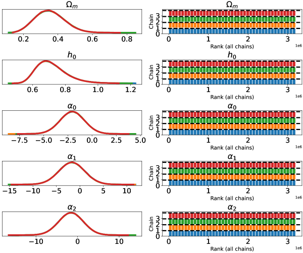
Figure 9: The random variables plotted here are the same as in the previous figures and in the same order. The right column shows the number of successful draws from the parameter space, which depends upon the sample size chosen as well as the prior theory. The four MCMC chains are plotted in different colors and the chains all are independent of each other.

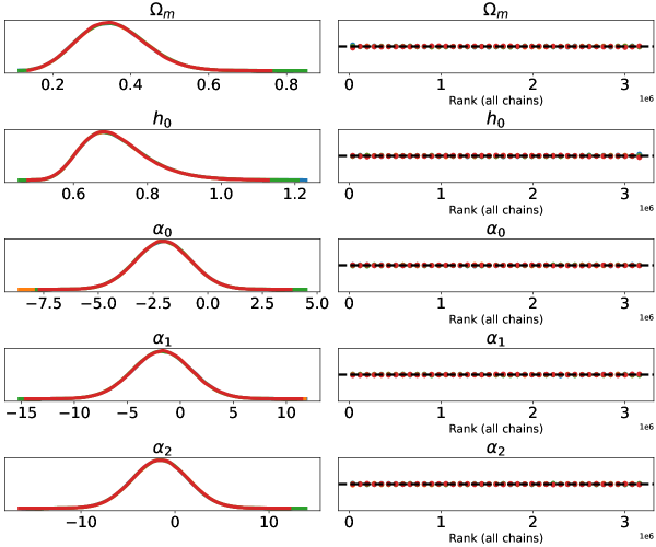
Figure 10: In this figure, the real Hubble parameter data-set is used to generate the plots. As in fig(5)m the left column consists of a smoothed histogram, using kernel density estimation of the marginal posteriors of each stochastic random variable. The right-hand column gives the auto-correlation for all the random variables for all the four independent chains, which are depicted with vertical lines.

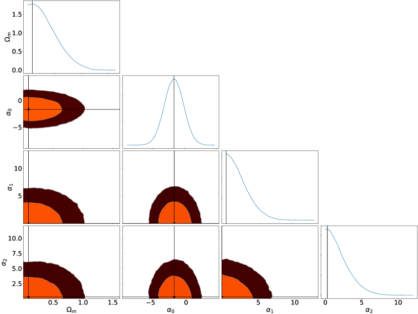
Figure 11: The plot shows the $1\sigma$ and $2\sigma$ contours for all the parameters along with their marginal probability density plots for the case of Pantheon data-set (Scolnic et al., 2022). For the plot we consider $[n_{d},M_{s}]=[200,100000]$. The models considered here are the $w_{CDM}$ model and the model described in eqn(1, 2).

The observable of the data-set is expressed as a polynomial over an initial basis function, which creates a coefficient space. The dimension of the coefficient space is the same as the number of initial basis functions. We select different patches in the coefficient space and do a $\chi^{2}$ calculation on each patch. For each patch, we get a minimum value of $\chi^{2}$. These minimum $\chi^{2}$ values for each patch give us the PCA data-matrix($\mathcal{D}$). We then calculate covariance matrix $\mathcal{C}$ of $\mathcal{D}$, from which the eigenvector matrix $\mathcal{E}$ is calculated. $\mathcal{E}$ is used to diagonalize $\mathcal{C}$ and omit the linear correlation of the data matrix. It also creates a new set of basis functions. The observable are then expressed in terms of the final basis function. With the help of these new basis functions, we create the new data-matrix $\mathcal{D}^{\prime}$. To select the value of the final basis number $M$, we compare the correlation matrix of $\mathcal{D}$ and $\mathcal{D^{\prime}}$. Comparison of correlation matrix also helps us to choose the better initial basis variable.

If the initial basis function is given by

$$G=(f_{1}(z),f_{2}(z),....,f_{N}(z)),$$

with $f_{i}(z)=f(z)^{(i-1)}$, the initial expression of the observable $\xi$ in terms of the independent variable $z$ is given by,

$$\xi_{ini}(z)=\sum_{i=1}^{N}b_{i}f(z)^{(i-1)}$$ (8)

The value of $N$ is the number of terms in the polynomial expression of $\xi_{ini}(z)$; it is also the dimension of coefficient space $\vec{b}$. The value of $N$ is determined by the correlation coefficient calculation (Kendall, 1938; Sharma et al., 2020). This value has to be large enough such that the function can capture most of the features from the observed data-set. To select the value of $N$, we calculate Pearson, Spearman, and Kendall correlation coefficients for the data-matrix $\mathcal{D}$ (Kendall, 1938; Kreyszig et al., 2011). The Pearson correlation coefficient gives the linear correlation that exists in the data-set. On the other hand, Spearman and Kendall correlation coefficients give the non-linear correlations of the data-set. For the Spearman correlation coefficient, we calculate the rank of the data-set. We arrange the ranks according to the numerical value, that is, we give rank 1 to the highest numerical value of the PCA data-set, rank 2 to the second highest, and so on. The Spearman correlation coefficient is the Pearson correlation coefficient of the rank variable of the data-set. Spearman correlation gives information about whether the dependent and independent variables are monotonically increasing or decreasing. For the Kendall correlation coefficient we find the concordant and disconcordant pairs. It gives the ordinal association between the variables (Kreyszig et al., 2011; Kendall, 1938).

We choose the smallest value of $N$ from the set of which the PCA data matrix gives us a higher value of Pearson Correlation coefficient compared to the Spearman and Kendall correlation coefficients. Only if the expression of the observable $\xi(z)$ in terms of the polynomial is exact, there would no correlation between the coefficients of the polynomial expression. Our motive is to break the correlation of the coefficient and obtain the polynomial expression of $\xi_{ini}(z)$ as closely as possible to the actual $\xi(z)$. After the reduction of the higher order Principal Component(PC)s the number of the terms in the polynomial of $\xi_{ini}(z)$ is $M$. The final functional form of the observable is,

$$\xi_{pca}(z)=\sum_{i=1}^{M}\kappa_{i}u_{i}(z)$$

where, $(u_{1}(z),u_{2}(z),....,u_{M}(z))$ and $U=G\mathcal{E}$. After the application of PCA, the dimension of the coefficient space $\vec{\kappa}$ is $M$.

In the earlier work we showed that a derived approach where the observable is obtained by the Principal Component Analysis and then reconstruction of dark energy equation of state parameter is an efficient method to reconstruct dark energy model than directly attempting to reconstruct it. For instance, while we can reconstruct the Hubble parameter $h(z)$ very well with PCA, the presence of a differentiation term in the equation given by eqn (3) which relates the EoS with $h(z)$ increases the errors in the reconstruction.

We address this problem by suggesting a modified approach to bypass the differentiation in the process of calculating EoS from the PCA reconstructed Hubble parameter and distance modulus function. This has been done by combining PCA with the Maximum Likelihood Estimation technique (MLE), using Markov Chain Monte Carlo (MCMC) to search for the best fit dark energy model to the PCA reconstructed Hubble parameter and distance modulus data-sets. We replace the observational part of the MLE calculation with best fit curve $h(z)$ and $\mu(z)$ as a function of redshift obtained via PCA. This method omits the dependencies on the number of observational data points. This analysis gives us the machinery to produce the most probable value of model parameters by constraining the theory with reconstructed PCA data. On the reconstructed curve of the observable, we perform the standard $\chi^{2}$ test. The errors are the error-functions, created from the co-variance matrix of PCA data-matrix (Huterer and Starkman, 2003; Sharma et al., 2020; Clarkson and Zunckel, 2010). The error is composed by the eigenvalues and eigenfunctions of the covariance matrix (Huterer and Starkman, 2003; Sharma et al., 2020; Clarkson and Zunckel, 2010). The eignevalues of the covariance matrix quantifies the error in the reconstruction of the observable $\xi(z)$. If $\lambda_{i}$ are the eigenvalues of the covariance matrix $\mathcal{C}$, then the error associated with each of the components is $\sigma(\alpha_{i})=\lambda_{i}^{1/2}$. For $M$ number of final terms we have the final error as,

$$\sigma(\xi(z_{a}))=\left[\sum_{i=1}^{M}\sigma^{2}(\alpha_{i})e^{2}_{i}(z_{a})\right]^{1/2}$$ (9)

Eqn(9) gives the error function for a particular reconstructed curve and we have the error as a function of redshift.

2.2 No-U-Turn sampler

To implement the MCMC search, we use the No-U-Turn sampler (NUTS) which is very effective in choosing the best parameter region. The No-U-Turn sampler is a modification of the Hamiltonian Monte Carlo(HMC), where the algorithm intrinsically selects the Leapfrog steps (Salvatier et al., 2016; Gelman and Rubin, 1992; Hoffman and Gelman, 2011). The selection of leapfrog steps is crucial in solving the Hamiltonian differential equations of the HMC.

To assess the MCMC methods, we have to measure how good the MCMC estimates are, which could be done using autocorrelation time, or by the variance of the estimate or the effective sample size. The autocorrelation of a variable measures the relationship between its present value and any past values we can access. If instead of one value, we compare the current series of values with the past historical data, it is called autocorrelation time series. The classical sample techniques like Metropolis-Hasting or Hamiltonian Monte Carlo create autocorrelated samples if the number of continuous parameters is very large. NUTS works very effectively in the case of parameter space which consists of a large number of continuous variables (Salvatier et al., 2016; Gelman and Rubin, 1992; Hoffman and Gelman, 2011). Based on the gradient of the log posterior density, NUTS takes advantage of where the regions of higher probability lie (Salvatier et al., 2016; Hoffman and Gelman, 2011). This is the reason NUTS achieves convergence faster on large problem sets than the traditional sample technique.

At every step, NUTS proceeds by creating a binary tree. In this binary tree, two particles representing progress in the forward and backward directions are created. If these two are represented as $(\mathbf{q_{n}^{+}},\mathbf{p_{n}^{+}})$ and $(\mathbf{q_{n}^{-}},\mathbf{p_{n}^{-}})$ then the NUTS can be given by,

$$(\mathbf{q}_{n}^{+}-\mathbf{q}_{n}^{-}).\mathbf{p}_{n}^{-}<0$$

$$(\mathbf{q}_{n}^{+}-\mathbf{q}_{n}^{-}).\mathbf{p}_{n}^{+}<0$$

NUTS is an improvement of Hamiltonian Monte Carlo sampling, where we move in the phase space of $\mathbf{q}$ and $\mathbf{p}$ in the elliptical path (Gelman and Rubin, 1992; Hoffman and Gelman, 2011). The motivation for introducing the momentum variable $\mathbf{p}$ is to ensure that we are exploring the greater area of the parameter space. This is done by moving in an elliptical contour, which we get after solving the dynamical Hamiltonian equation. In NUTS, when we move half of the elliptical path, the sign of the momentum and the position variables are changed, and we stop. This makes the NUTS more efficient than HMC, where there is no way to ascertain if we are moving in the already explored region of parameter space.

We choose the value of the total sample points $M_{s}$ by checking the convergence limit using Gelman-Rubin statistic (Salvatier et al., 2016). Gelman-Rubin statistic for convergence is based on the notion that multiple convergence chain appears to be similar to each other; otherwise, they will not converge. It is a standard method to run multiple MCMC chains to test for convergence. Scale reduction factor $\hat{r_{o}}$ is used to check the Gelman-Rubin convergence. There are two main ways the sequences of MCMC iterations fail to converge. In one case, the chains run in different parts, which have drastic differences in posterior probability densities of the target distribution. On the other, the chains fail to attain convergence. We change the value of $M_{s}$ until we get $\hat{r_{o}}=1$.

data-type	parameter	1$\sigma$	2$\sigma$
simulated	$\Omega_{m}$	[0.238, 0.415]	[0.169, 0.508]
	$h_{0}$	[0.55, 0.7161]	[0.496, 0.847]
	$\alpha_{0}$	[-3.01, -0.48]	[-4.24, 0.739]
	$\alpha_{1}$	[-4.379, 1.145]	[-7.047, 3.85]
	$\alpha_{2}$	[-4.501, 1.394]	[-7.314, 4.3]
real	$\Omega_{m}$	[0.259, 0.43]	[0.19, 0.52]
	$h_{0}$	[0.61, 0.778]	[0.55, 0.903]
	$\alpha_{0}$	[-3.32, -0.81]	[-4.54, 0.421]
	$\alpha_{1}$	[-4.492, 1.023]	[-7.143, 3.75]
	$\alpha_{2}$	[-4.53, 1.36]	[-7.39, 4.198]

Table 1: This table gives the 1$\sigma$ and 2$\sigma$ ranges for parameters, $h_{0}$, $\Omega_{m}$, $\alpha_{0}$, $\alpha_{1}$ and $\alpha_{2}$, where $\vec{\alpha}$ are the parameters of dark energy equation of state.

data-type and model	parameter	1$\sigma$	2$\sigma$
pantheon ($w_{CDM}$)	$\Omega_{m}$	[0.0165, 0.4363]	[$\mathcal{O}(-5)$, 0.7882]
	$\alpha_{0}$	[-3.27, -0.417]	[-4.84, 0.63]
pantheon ($w_{model}$)	$\Omega_{m}$	[$\mathcal{O}(-6)$, 0.426]	[$\mathcal{O}(-6)$, 0.817]
	$\alpha_{0}$	[-3.131, -0.159]	[-4.553, 1.298]
	$\alpha_{1}$	[0.000112, 2.613]	[$\mathcal{O}$(-5), 5.347]
	$\alpha_{2}$	[$\mathcal{O}$(-5), 2.46]	[$\mathcal{O}$(-7), 5.12]

Table 2: This table gives the 1$\sigma$ and 2$\sigma$ ranges for parameters, $\Omega_{m}$ and $\vec{\alpha}$ For For $\alpha_{0}$ for $w_{CDM}$ as well as the dark energy model of eqn(2). Here $\vec{\alpha}$ are the parameters of dark energy equation of state parameter. Here we use the Pantheon data-set, with $h_{0}=0.7$. Here $[n_{d},M_{s}]=[200,100000]$

3 Results

We do the analysis described above first for Hubble parameter and then for Pantheon data-set. For Hubble parameter we show the results of both simulated as well as the real data-set. The simulated data-set is created using the same parameter values as is fixed by (Planck Collaboration et al., 2018). For the simulated $\Lambda$CDM data-set we have fixed the values of cosmological parameters as, $\Omega_{m}=0.3$ and $h_{0}=0.684$. We test the validity of our method and check if these values are picked up by the analysis. We then apply the method to the real data-set, namely the Cosmic-Chronometer data-set (Zhang et al., 2014; Simon et al., 2005; Moresco et al., 2012; Ratsimbazafy et al., 2017; Moresco, 2015) as well as Pantheon data-set Scolnic et al. (2022) and compare with the usual likelihood analysis results.

To get the reconstructed curve of reduced Hubble parameter and distance modulus we use $f(z)=\frac{z}{(1+z)}$ as initial basis function for simulated data as well as observational dataset. This initial basis function gives the best reconstruction as shown in (Sharma et al., 2020). Here, we have the freedom to choose the value of $n_{d}$, which is the number of data points in the observed part of MLE. We run the Markov Chain Monte Carlo (MCMC) chain to search for minimum $\chi^{2}$, which give us the likelihood of the PCA data-set. In the MCMC analysis, for Hubble parameter data-set we use normal priors $\mathcal{N}(0.70,0.2)$ and $\mathcal{N}(0.35,0.1)$ for reduced Hubble constant $h_{0}$ and $\Omega_{m}$ respectively. For the DE parameters, $\vec{\alpha}$ we take $\mathcal{N}(0,3)$. Here, $\mathcal{N}(x_{mean},x_{mode})$ represents the normal probability density function with $x_{mean}$ and spread of $x_{mode}$. For Pantheon data-set, we fix the reduced Hubble constant and absolute magnitude at $0.7$ and $-19.3$ respectively, as discussed in Riess et al. (2022) and later in Perivolaropoulos and Skara (2023). In the MLE part we take half normal with standard deviation of $0.4$ as a prior of $\Omega_{m}$ and for $\vec{\alpha}$ we take $\mathcal{N}(-2,1.5)$.

We choose the largest possible value for $n_{d}$ which is limited by the computing power. We then check the results for different values of $n_{d}$ and $M_{s}$ and find out the mean, median and mode of the posterior distribution. For $m=3$ eqn(2), we do the analysis for different values of $n_{d}$ and $M_{s}$. $m=3$ is the CPL parameterization along with the next order term (Chevallier and Polarski, 2001; Linder, 2003). $n_{d}$ is varied in the range 100 to 800 whereas $M_{s}$ in the range 1000 to 800000 and finds out mean, median, and mode as well as 1$\sigma$ and 2$\sigma$ ranges of $\omega_{m}$, $h_{0}$, $\vec{\alpha}$.

In Figures 3 and 1, we show results for $n_{d}=600$, where we fix the number of sample points at $M_{s}=80,0000$. This particular choice of $n_{d}$ and $M_{s}$ gives us the closest approximation of the model parameters for the simulated Hubble parameter data and we see that about this value of $n_{d}$ and $M_{s}$ we get the smallest variation in $1\sigma$ and $2\sigma$ ranges of the model parameters. In particular for $(n_{d},M_{s})=(600,800000)\&(1000,50000)$ the difference in $1\sigma$ and $2\sigma$ ranges are of the order of $\mathcal{O}(-1)$ for $\vec{\alpha}$ and $\mathcal{O}(-2)$ or less for $\Omega_{m}$ and $h_{0}$. For Hubble parameter data-set, to create the simulated data we assume $h_{0}=0.685$ and $\Omega_{m}=0.3$, while the mean of the posterior of $h_{0}$ and $\Omega_{m}$ from the algorithm are $h_{0}=0.68$ and $\Omega_{m}=0.34$, which are very close to the assumed values, $h_{0}=0.685$ and $\Omega_{m}=0.3$. In table 1 we show the $1\sigma$, $2\sigma$ ranges for the parameters of the theory, eqn(1). Mean of the posterior of $h_{0}$ and $\Omega_{m}$ for the real Hubble parameter data from the algorithm are $h_{0}=0.71$ and $\Omega_{m}=0.35$ respectively. Similarly, in table 2 we present our result for Pantheon data-set Scolnic et al. (2022). We show our results for $w_{CDM}$ and for the model of eqn(2) in fig(11). For Pantheon data-set, we present our results for $(n_{d},M_{S})=(200,100000)$.

It is also evident from the fig(3, 2, 4, 11) that $w(z)=-1$ is well within the $1\sigma$ range of $w(z)$ parameters($\vec{\alpha}$). The plot of $w(z)$ and $\rho(z)/\rho_{0}$ are similar for both real and simulated data-set. Difference in $w(z)$ and $\rho(z)/\rho_{0}$ curve between simulated and real Hubble parameter data are 0.442 and 0.024 respectively. Here, $\rho(z)$ and $\rho_{0}$ are the total energy density at redshift $z$ and at present. The dark energy density plot, $\rho^{\prime}(z)/\rho^{\prime}_{0}$ vs $z$, for simulated and real Hubble parameter data-set are also similar and the maximum difference between them for Hubble parameter data-set is $0.36$.

For each MCMC run, we calculate the Gelman-Rubin convergence factor $\hat{r_{o}}$. In the MCMC run for both the real and simulated Hubble parameter data-set, with $(n_{d},M_{s})=(600,800000)$, the value of $\hat{r_{o}}$ is $1$. For Pantheon MCMC run $(n_{d},M_{s})=(200,100000)$ gives the value of $\hat{r_{o}}=1$. To check the convergence we not only check the $\hat{r_{o}}$ factor and eliminate those iterations which do not satisfy the $\hat{r_{o}}\approx 1$ criteria but we also check the trace plots, rank bar plots and the rank vertical bar plots of the posterior sampling for visual confirmations (Gelman and Rubin, 1992; Brooks and Gelman, 1998; Cowles and Carlin, 1996).

Fig 5, 6, and 7 shows the convergence of the MCMC chains for the simulated Hubble parameter data-set. These plots are created for $(n_{d},M_{s})=(600,800000)$. The convergence and the ability to draw successful samples from the parameter space is apparent for $(n_{d},M_{s})=(600,800000)$ set in the case of Hubble parameter data-set. The same application for the real Hubble parameter data is shown in fig 8, 9, and 10. Fig(7, 10) gives the auto-correlation of different parameters for different MCMC chains. We see from fig(7, 10) that auto-correlation of the parameters for different chains are zero. For Pantheon data-set also, the auto-correlation as well as the trace plots are similar, and shows the convergence of the MCMC chain. The comparison between NUTS with the classical Metropolis-Hastings (MH) as well as the Hamiltonian Monte Carlo sampler (HMC) is shown in A.

4 Conclusions

In this paper, we combine the Principal Component Analysis reconstruction with the Markov Chain Monte Carlo tool to determine cosmological parameters. We assume the Taylor series expansion of the equation of state parameter in terms of the scale factor as the parameterization of the dark energy equation of state. When the method of PCA along with correlation coefficient calculation reconstruction is combined with MCMC tool, we have the freedom of selecting the number of points in the observational part of maximum likelihood method. We use the No U Turn Sampler for this analysis.

We first test the method on simulated data and check if the values assumed for the cosmological parameters are reconstructed effectively. We see that the predictions for the model parameters are consistent with the assumed values. The parameter estimation does not depend strongly on the prior probability assumption, and the idea can be generalized to other data-sets as well as different sampling techniques. The relation between the Hubble parameter and the equation of state of dark energy also contains the first differentiation of the Hubble parameter, which introduces an unwanted error in the equation of state predictions. Similarly, for Pantheon data-set the relation between the distance modulus and EoS of dark energy contains first and second order differentiation.

The present method eliminates the error that arises from the first and higher order differentiation of the observable to infer the value and ranges of the Equation of State of dark energy. In this work, we only use the error function that comes directly from the PCA algorithm, and one can use different error functions in the error part of the MLE as well. It is clear from the results that the allowed range of cosmological parameters is consistent with other analysis and cosmological constant model is well within the allowed range of models for both the Hubble parameter and Pantheon data-set. Here the advantage is that the full functional form of the dataset observable is obtained; in the present work the Hubble parameter and distance modulus as a function of redshift are determined. The second step is deriving the dark energy equation of state parameter. The method discussed here can be used as a model selection tool and in those data-sets with fewer data-points.

Data Availability

The observational data-set used in the analysis is publicly available and duly referred to is the text (Zhang et al., 2014; Simon et al., 2005; Moresco et al., 2012; Ratsimbazafy et al., 2017; Moresco, 2015; Scolnic et al., 2022). The simulated data-set can be created by using the standard $\Lambda CDM$ model, using eqn(1-6) of the text.

Appendix A Maximum Likelihood analysis with Hamiltonian Monte Carlo and Metropolis Hasting analysis

Here, we include the plots for Metropolis Hasting algorithm (MH), fig(12) and fig(13), as well as the plots for the Hamiltonian Monte Carlo algorithm, fig(14) and fig(15). It is clear from the figures that, NUTS and Hamiltonian Monte Carlo sampler (HMC) perform better than Metropolis Hastings sampler (MH). It has been explicitly shown in (Hoffman and Gelman, 2011) that the NUTS algorithm is more efficient. For a comparison we use the same number of simulated data points $n_{d}$ as well as the sample points $M_{s}$ as in NUTS simulation, these are $(n_{d},M_{s})=(600,800000)$. To compare HMC sampler and NUTS, NUTS is better than HMC as NUTS picks up the leapfrog steps, and it stops automatically when the NUTS conditions are satisfied.

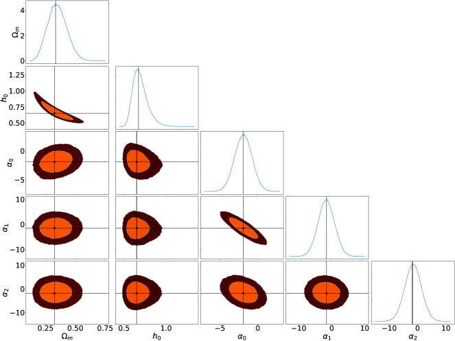
Figure 12: The plots show the $1\sigma$ and $2\sigma$ contours for all the parameters as well as only for the EoS parameters along with their marginal probability density plots. Both the plots are for the case of simulated $\Lambda CDM$ Hubble parameter data-set and we use Matropolis-Hasting (MH) algorithm in the MLE section of the reconstruction.

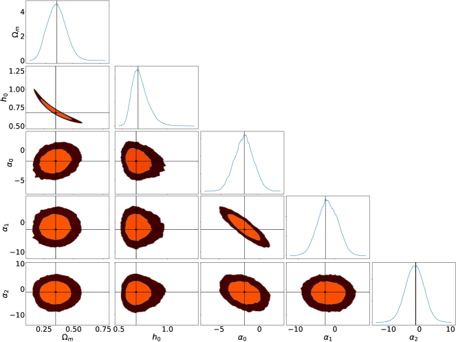
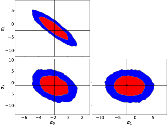
Figure 13: As in figure(12), both the plots are for Metropolis Hasting algorithm, and we use the real Hubble parameter data in the present case. From top to bottom plots are for the $1\sigma$ and $2\sigma$ contours for all the parameters as well as only for the EoS parameters along with their marginal probability density plots, respectively.

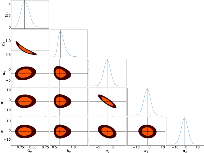
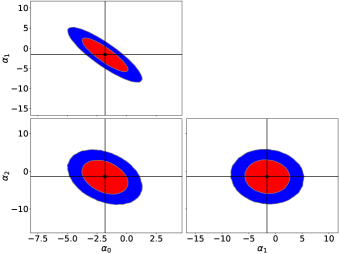
Figure 14: These plots show the $1\sigma$ and $2\sigma$ contours for all the parameters as well as only for the EoS parameters along with their marginal probability density plots. Both the plots are for the case of simulated $\Lambda CDM$ Hubble parameter data-set and we use Hamiltonian Monte Carlo algorithm in the MLE section of the reconstruction. For comparison we use the same value of $(n_{d},M_{s})=(600,800000)$.

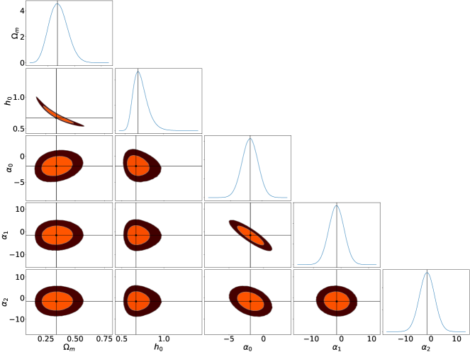
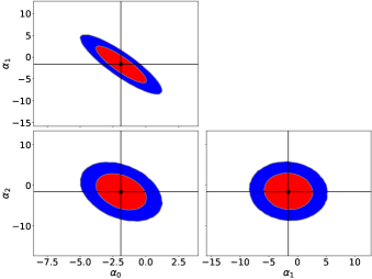
Figure 15: As in the figures above, both the plots are for Hamiltonian Monte Carlo algorithm, and we use the real Hubble parameter data in the present case. From top to bottom plots are for the $1\sigma$ and $2\sigma$ contours for all the parameters as well as only for the EoS parameters along with their marginal probability density plots, respectively. For comparison purpose here also, we use the same value of $(n_{d},M_{s})=(600,800000)$

References

- Albrecht et al. (2006) Albrecht, A., Bernstein, G., Cahn, R., Freedman, W.L., Hewitt, J., Hu, W., Huth, J., Kamionkowski, M., Kolb, E.W., Knox, L., Mather, J.C., Staggs, S., Suntzeff, N.B., 2006. Report of the Dark Energy Task Force. arXiv e-prints , astro–ph/0609591arXiv:astro-ph/0609591.
- Arjona and Nesseris (2020) Arjona, R., Nesseris, S., 2020. Machine Learning and cosmographic reconstructions of quintessence and the Swampland conjectures. arXiv e-prints , arXiv:2012.12202arXiv:2012.12202.
- Bagla et al. (2003) Bagla, J.S., Jassal, H.K., Padmanabhan, T., 2003. Cosmology with tachyon field as dark energy. Phys. Rev. D 67, 063504. URL: https://link.aps.org/doi/10.1103/PhysRevD.67.063504, doi:10.1103/PhysRevD.67.063504.
- Banerjee et al. (2021) Banerjee, A., Cai, H., Heisenberg, L., Colgáin, E.Ó., Sheikh-Jabbari, M.M., Yang, T., 2021. Hubble sinks in the low-redshift swampland. Phys. Rev. D 103, L081305. doi:10.1103/PhysRevD.103.L081305, arXiv:2006.00244.
- Bellomo et al. (2020) Bellomo, N., Bernal, J.L., Scelfo, G., Raccanelli, A., Verde, L., 2020. Beware of commonly used approximations. Part I. Errors in forecasts. J. Cosmology Astropart. Phys 2020, 016. doi:10.1088/1475-7516/2020/10/016, arXiv:2005.10384.
- Bernal et al. (2020) Bernal, J.L., Bellomo, N., Raccanelli, A., Verde, L., 2020. Beware of commonly used approximations. Part II. Estimating systematic biases in the best-fit parameters. J. Cosmology Astropart. Phys 2020, 017. doi:10.1088/1475-7516/2020/10/017, arXiv:2005.09666.
- Brooks and Gelman (1998) Brooks, S.P., Gelman, A., 1998. General methods for monitoring convergence of iterative simulations. Journal of Computational and Graphical Statistics 7, 434–455. URL: https://www.tandfonline.com/doi/abs/10.1080/10618600.1998.10474787, doi:10.1080/10618600.1998.10474787, arXiv:https://www.tandfonline.com/doi/pdf/10.1080 /10618600.1998.10474787.
- Caldwell et al. (1998) Caldwell, R.R., Dave, R., Steinhardt, P.J., 1998. Cosmological imprint of an energy component with general equation of state. Phys. Rev. Lett. 80, 1582–1585. URL: https://link.aps.org/doi/10.1103/PhysRevLett.80.1582, doi:10.1103/PhysRevLett.80.1582.
- Caldwell and Linder (2005) Caldwell, R.R., Linder, E.V., 2005. The Limits of quintessence. Phys. Rev. Lett. 95, 141301. doi:10.1103/PhysRevLett.95.141301, arXiv:astro-ph/0505494.
- Carroll (2001) Carroll, S.M., 2001. The Cosmological constant. Living Rev. Rel. 4, 1. doi:10.12942/lrr-2001-1, arXiv:astro-ph/0004075.
- Carroll et al. (1992) Carroll, S.M., Press, W.H., Turner, E.L., 1992. The cosmological constant. Annual Review of Astronomy and Astrophysics 30, 499–542. URL: https://doi.org/10.1146/annurev.aa.30.090192.002435, doi:10.1146/annurev.aa.30.090192.002435.
- Chevallier and Polarski (2001) Chevallier, M., Polarski, D., 2001. Accelerating universes with scaling dark matter. Int. J. Mod. Phys. D10, 213–224. doi:10.1142S0218271801000822, arXiv:gr-qc0009008.
- Chevallier and Polarski (2001) Chevallier, M., Polarski, D., 2001. Accelerating Universes with Scaling Dark Matter. International Journal of Modern Physics D 10, 213–223. doi:10.1142/S0218271801000822, arXiv:gr-qc/0009008.
- Clarkson and Zunckel (2010) Clarkson, C., Zunckel, C., 2010. Direct Reconstruction of Dark Energy. Phys. Rev. Lett. 104, 211301. doi:10.1103/PhysRevLett.104.211301, arXiv:1002.5004.
- Coble et al. (1997) Coble, K., Dodelson, S., Frieman, J.A., 1997. Dynamical models of structure formation. Phys. Rev. D 55, 1851–1859. URL: https://link.aps.org/doi/10.1103/PhysRevD.55.1851, doi:10.1103/PhysRevD.55.1851.
- Copeland et al. (1998) Copeland, E.J., Liddle, A.R., Wands, D., 1998. Exponential potentials and cosmological scaling solutions. Phys. Rev. D57, 4686–4690. doi:10.1103/PhysRevD.57.4686, arXiv:gr-qc/9711068.
- Copeland et al. (2006) Copeland, E.J., Sami, M., Tsujikawa, S., 2006. Dynamics of dark energy. Int. J. Mod. Phys. D15, 1753–1936. doi:10.1142/S021827180600942X, arXiv:hep-th/0603057.
- Cowles and Carlin (1996) Cowles, M.K., Carlin, B.P., 1996. Markov chain monte carlo convergence diagnostics: A comparative review. Journal of the American Statistical Association 91, 883–904. URL: https://www.tandfonline.com/doi/abs/10.1080/01621459.1996.10476956, doi:10.1080/01621459.1996.10476956, arXiv:https://www.tandfonline.com/doi/pdf/ 10.1080/01621459.1996.10476956.
- Crittenden et al. (2009) Crittenden, R.G., Pogosian, L., Zhao, G.B., 2009. Investigating dark energy experiments with principal components. JCAP 0912, 025. doi:10.1088/1475-7516/2009/12/025, arXiv:astro-ph/0510293.
- Di Valentino et al. (2017) Di Valentino, E., Melchiorri, A., Linder, E.V., Silk, J., 2017. Constraining Dark Energy Dynamics in Extended Parameter Space. Phys. Rev. D96, 023523. doi:10.1103/PhysRevD.96.023523, arXiv:1704.00762.
- Ellis (2003) Ellis, J., 2003. Dark matter and dark energy: summary and future directions. Philosophical Transactions of the Royal Society of London A: Mathematical, Physical and Engineering Sciences 361, 2607–2627. URL: http://rsta.royalsocietypublishing.org/content/361/1812/2607, doi:10.1098/rsta.2003.1297.
- Frieman et al. (2008) Frieman, J.A., Turner, M.S., Huterer, D., 2008. Dark energy and the accelerating universe. Annual Review of Astronomy and Astrophysics 46, 385–432. URL: https://doi.org/10.1146/annurev.astro.46.060407.145243, doi:10.1146/annurev.astro.46.060407.145243.
- Gelman and Rubin (1992) Gelman, A., Rubin, D.B., 1992. Inference from iterative simulation using multiple sequences. Statistical Science 7, 457–472. URL: http://www.jstor.org/stable/2246093.
- Gong and Wang (2007) Gong, Y.G., Wang, A., 2007. Reconstruction of the deceleration parameter and the equation of state of dark energy. Phys. Rev. D75, 043520. doi:10.1103/PhysRevD.75.043520, arXiv:astro-ph/0612196.
- Hart and Chluba (2019) Hart, L., Chluba, J., 2019. Improved model-independent constraints on the recombination era and development of a direct projection method. arXiv e-prints , arXiv:1912.04682arXiv:1912.04682.
- Hart and Chluba (2022) Hart, L., Chluba, J., 2022. Varying fundamental constants principal component analysis: additional hints about the Hubble tension. MNRAS 510, 2206–2227. doi:10.1093/mnras/stab2777, arXiv:2107.12465.
- Hoffman and Gelman (2011) Hoffman, M.D., Gelman, A., 2011. The No-U-Turn Sampler: Adaptively Setting Path Lengths in Hamiltonian Monte Carlo. arXiv e-prints , arXiv:1111.4246arXiv:1111.4246.
- Hojjati et al. (2012) Hojjati, A., Zhao, G.B., Pogosian, L., Silvestri, A., Crittenden, R., Koyama, K., 2012. Cosmological tests of general relativity: A principal component analysis. Phys. Rev. D 85, 043508. doi:10.1103/PhysRevD.85.043508, arXiv:1111.3960.
- Huterer and Cooray (2005) Huterer, D., Cooray, A., 2005. Uncorrelated estimates of dark energy evolution. Phys. Rev. D 71, 023506. doi:10.1103/PhysRevD.71.023506, arXiv:astro-ph/0404062.
- Huterer and Peiris (2007) Huterer, D., Peiris, H.V., 2007. Dynamical behavior of generic quintessence potentials: Constraints on key dark energy observables. Phys. Rev. D75, 083503. doi:10.1103/PhysRevD.75.083503, arXiv:astro-ph/0610427.
- Huterer and Starkman (2003) Huterer, D., Starkman, G., 2003. Parametrization of Dark-Energy Properties: A Principal-Component Approach. Phys. Rev. Lett. 90, 031301. doi:10.1103/PhysRevLett.90.031301, arXiv:astro-ph/0207517.
- Ishida and de Souza (2011) Ishida, E.E.O., de Souza, R.S., 2011. Hubble parameter reconstruction from a principal component analysis: minimizing the bias. A&A 527, A49. doi:10.1051/0004-6361/201015281, arXiv:1012.5335.
- Jassal (2009) Jassal, H.K., 2009. A comparison of perturbations in fluid and scalar field models of dark energy. Phys. Rev. D79, 127301. doi:10.1103/PhysRevD.79.127301, arXiv:0903.5370.
- Jassal et al. (2005) Jassal, H.K., Bagla, J.S., Padmanabhan, T., 2005. WMAP constraints on low redshift evolution of darkenergy. Mon. Not. Roy. Astron. Soc. 356, L11–L16. doi:10.1111/j.1745-3933.2005.08577.x, arXiv:astro-ph/0404378.
- Kendall (1938) Kendall, 1938. A NEW MEASURE OF RANK CORRELATION. Biometrika 30, 81–93. URL: https://doi.org/10.1093/biomet/30.1-2.81, doi:10.1093/biomet/30.1-2.81, arXiv:https://academic.oup.com/biomet/ article-pdf/30/1-2/81/423380/30-1-2-81.pdf.
- Kreyszig et al. (2011) Kreyszig, E., Kreyszig, H., Norminton, E.J., 2011. Advanced engineering mathematics. Tenth ed., Wiley, Hoboken, N.J. URL: http://www.worldcat.org/search?qt=worldcat_org_all&q=9780470458365.
- Lee et al. (2022) Lee, B.H., Lee, W., Ó Colgáin, E., Sheikh-Jabbari, M.M., Thakur, S., 2022. Is local H 0 at odds with dark energy EFT? J. Cosmology Astropart. Phys 2022, 004. doi:10.1088/1475-7516/2022/04/004, arXiv:2202.03906.
- Linder (2003) Linder, E.V., 2003. Exploring the expansion history of the universe. Phys. Rev. Lett. 90, 091301. doi:10.1103/PhysRevLett.90.091301, arXiv:astro-ph/0208512.
- Linder (2003) Linder, E.V., 2003. Exploring the Expansion History of the Universe. Phys. Rev. Lett. 90, 091301. doi:10.1103/PhysRevLett.90.091301, arXiv:astro-ph/0208512.
- Linder (2006) Linder, E.V., 2006. The paths of quintessence. Phys. Rev. D73, 063010. doi:10.1103/PhysRevD.73.063010, arXiv:astro-ph/0601052.
- Linder (2008) Linder, E.V., 2008. Mapping the cosmological expansion. Reports on Progress in Physics 71, 056901. doi:10.1088/0034-4885/71/5/056901, arXiv:0801.2968.
- Linder (2008) Linder, E.V., 2008. The Dynamics of Quintessence, The Quintessence of Dynamics. Gen. Rel. Grav. 40, 329–356. doi:10.1007/s10714-007-0550-z, arXiv:0704.2064.
- Miranda and Dvorkin (2018) Miranda, V., Dvorkin, C., 2018. Model-independent predictions for smooth cosmic acceleration scenarios. Phys. Rev. D 98, 043537. doi:10.1103/PhysRevD.98.043537, arXiv:1712.04289.
- Moresco (2015) Moresco, M., 2015. Raising the bar: new constraints on the Hubble parameter with cosmic chronometers at z ~2. MNRAS 450, L16–L20. doi:10.1093/mnrasl/slv037, arXiv:1503.01116.
- Moresco et al. (2012) Moresco, M., Verde, L., Pozzetti, L., Jimenez, R., Cimatti, A., 2012. New constraints on cosmological parameters and neutrino properties using the expansion rate of the Universe to z 1.75. JCAP 1207, 053. doi:10.1088/1475-7516/2012/07/053, arXiv:1201.6658.
- Mukherjee (2016) Mukherjee, A., 2016. Acceleration of the universe: a reconstruction of the effective equation of state. Mon. Not. Roy. Astron. Soc. 460, 273–282. doi:10.1093/mnras/stw964, arXiv:1605.08184.
- Nair and Jhingan (2013) Nair, R., Jhingan, S., 2013. Is dark energy evolving? J. Cosmology Astropart. Phys 2013, 049. doi:10.1088/1475-7516/2013/02/049, arXiv:1212.6644.
- Nesseris and García-Bellido (2013) Nesseris, S., García-Bellido, J., 2013. Comparative analysis of model-independent methods for exploring the nature of dark energy. Phys. Rev. D 88, 063521. doi:10.1103/PhysRevD.88.063521, arXiv:1306.4885.
- Nesseris and Perivolaropoulos (2004) Nesseris, S., Perivolaropoulos, L., 2004. Comparison of cosmological models using recent supernova data. Phys. Rev. D 70, 043531. doi:10.1103/PhysRevD.70.043531, arXiv:astro-ph/0401556.
- Nesseris and Perivolaropoulos (2005) Nesseris, S., Perivolaropoulos, L., 2005. Comparison of the legacy and gold type Ia supernovae dataset constraints on dark energy models. Phys. Rev. D 72, 123519. doi:10.1103/PhysRevD.72.123519, arXiv:astro-ph/0511040.
- Nesseris and Perivolaropoulos (2007) Nesseris, S., Perivolaropoulos, L., 2007. Crossing the phantom divide: theoretical implications and observational status. J. Cosmology Astropart. Phys 2007, 018. doi:10.1088/1475-7516/2007/01/018, arXiv:astro-ph/0610092.
- Padmanabhan (2002) Padmanabhan, T., 2002. Accelerated expansion of the universe driven by tachyonic matter. Phys. Rev. D 66, 021301. URL: https://link.aps.org/doi/10.1103/PhysRevD.66.021301, doi:10.1103/PhysRevD.66.021301.
- Padmanabhan (2003) Padmanabhan, T., 2003. Cosmological constant: The Weight of the vacuum. Phys. Rept. 380, 235–320. doi:10.1016/S0370-1573(03)00120-0, arXiv:hep-th/0212290.
- Peebles and Ratra (2003) Peebles, P.J.E., Ratra, B., 2003. The Cosmological constant and dark energy. Rev. Mod. Phys. 75, 559–606. doi:10.1103/RevModPhys.75.559, arXiv:astro-ph/0207347. [,592(2002)].
- Perivolaropoulos and Skara (2023) Perivolaropoulos, L., Skara, F., 2023. On the homogeneity of SnIa absolute magnitude in the Pantheon+ sample. MNRAS doi:10.1093/mnras/stad451, arXiv:2301.01024.
- Planck Collaboration et al. (2018) Planck Collaboration, Aghanim, N., Akrami, Y., Ashdown, M., Aumont, J., Baccigalupi, C., Ballardini, M., Banday, A.J., Barreiro, R.B., Bartolo, N., Basak, S., Battye, R., Benabed, K., Bernard, J.P., Bersanelli, M., Bielewicz, P., Bock, J.J., Bond, J.R., Borrill, J., Bouchet, F.R., Boulanger, F., Bucher, M., Burigana, C., Butler, R.C., Calabrese, E., Cardoso, J.F., Carron, J., Challinor, A., Chiang, H.C., Chluba, J., Colombo, L.P.L., Combet, C., Contreras, D., Crill, B.P., Cuttaia, F., de Bernardis, P., de Zotti, G., Delabrouille, J., Delouis, J.M., Di Valentino, E., Diego, J.M., Doré, O., Douspis, M., Ducout, A., Dupac, X., Dusini, S., Efstathiou, G., Elsner, F., Enßlin, T.A., Eriksen, H.K., Fantaye, Y., Farhang, M., Fergusson, J., Fernandez-Cobos, R., Finelli, F., Forastieri, F., Frailis, M., Fraisse, A.A., Franceschi, E., Frolov, A., Galeotta, S., Galli, S., Ganga, K., Génova-Santos, R.T., Gerbino, M., Ghosh, T., González-Nuevo, J., Górski, K.M., Gratton, S., Gruppuso, A., Gudmundsson, J.E., Hamann, J., Handley, W., Hansen, F.K., Herranz, D., Hildebrandt, S.R., Hivon, E., Huang, Z., Jaffe, A.H., Jones, W.C., Karakci, A., Keihänen, E., Keskitalo, R., Kiiveri, K., Kim, J., Kisner, T.S., Knox, L., Krachmalnicoff, N., Kunz, M., Kurki-Suonio, H., Lagache, G., Lamarre, J.M., Lasenby, A., Lattanzi, M., Lawrence, C.R., Le Jeune, M., Lemos, P., Lesgourgues, J., Levrier, F., Lewis, A., Liguori, M., Lilje, P.B., Lilley, M., Lindholm, V., López-Caniego, M., Lubin, P.M., Ma, Y.Z., Macías-Pérez, J.F., Maggio, G., Maino, D., Mandolesi, N., Mangilli, A., Marcos-Caballero, A., Maris, M., Martin, P.G., Martinelli, M., Martínez-González, E., Matarrese, S., Mauri, N., McEwen, J.D., Meinhold, P.R., Melchiorri, A., Mennella, A., Migliaccio, M., Millea, M., Mitra, S., Miville-Deschênes, M.A., Molinari, D., Montier, L., Morgante, G., Moss, A., Natoli, P., Nørgaard-Nielsen, H.U., Pagano, L., Paoletti, D., Partridge, B., Patanchon, G., Peiris, H.V., Perrotta, F., Pettorino, V., Piacentini, F., Polastri, L., Polenta, G., Puget, J.L., Rachen, J.P., Reinecke, M., Remazeilles, M., Renzi, A., Rocha, G., Rosset, C., Roudier, G., Rubiño-Martín, J.A., Ruiz-Granados, B., Salvati, L., Sandri, M., Savelainen, M., Scott, D., Shellard, E.P.S., Sirignano, C., Sirri, G., Spencer, L.D., Sunyaev, R., Suur-Uski, A.S., Tauber, J.A., Tavagnacco, D., Tenti, M., Toffolatti, L., Tomasi, M., Trombetti, T., Valenziano, L., Valiviita, J., Van Tent, B., Vibert, L., Vielva, P., Villa, F., Vittorio, N., Wand elt, B.D., Wehus, I.K., White, M., White, S.D.M., Zacchei, A., Zonca, A., 2018. Planck 2018 results. VI. Cosmological parameters. arXiv e-prints , arXiv:1807.06209arXiv:1807.06209.
- R Core Team (2013) R Core Team, 2013. R: A Language and Environment for Statistical Computing. R Foundation for Statistical Computing. Vienna, Austria. URL: http://www.R-project.org/.
- Rajvanshi and Bagla (2019) Rajvanshi, M.P., Bagla, J.S., 2019. Reconstruction of dynamical dark energy potentials: Quintessence, tachyon and interacting models. Journal of Astrophysics and Astronomy 40, 44. doi:10.1007/s12036-019-9613-2, arXiv:1905.01103.
- Ratra and Peebles (1988) Ratra, B., Peebles, P.J.E., 1988. Cosmological Consequences of a Rolling Homogeneous Scalar Field. Phys. Rev. D37, 3406. doi:10.1103/PhysRevD.37.3406.
- Ratsimbazafy et al. (2017) Ratsimbazafy, A.L., Loubser, S.I., Crawford, S., Cress, C.M., Bassett, B.A., Nichol, R. C.and Väisänen, P., 2017. Age-dating Luminous Red Galaxies observed with the Southern African Large Telescope. Mon. Not. Roy. Astron. Soc. 467, 3239–3254. doi:10.1093/mnras/stx301, arXiv:1702.00418.
- Riess et al. (2022) Riess, A.G., Yuan, W., Macri, L.M., Scolnic, D., Brout, D., Casertano, S., Jones, D.O., Murakami, Y., Anand, G.S., Breuval, L., Brink, T.G., Filippenko, A.V., Hoffmann, S., Jha, S.W., D’arcy Kenworthy, W., Mackenty, J., Stahl, B.E., Zheng, W., 2022. A Comprehensive Measurement of the Local Value of the Hubble Constant with 1 km s-1 Mpc-1 Uncertainty from the Hubble Space Telescope and the SH0ES Team. ApJ 934, L7. doi:10.3847/2041-8213/ac5c5b, arXiv:2112.04510.
- Sahni and Starobinsky (2000) Sahni, V., Starobinsky, A., 2000. The Case for a Positive Cosmological -Term. International Journal of Modern Physics D 9, 373–443. doi:10.1142/S0218271800000542, arXiv:astro-ph/9904398.
- Salvatier et al. (2016) Salvatier, J., Wiecki, T.V., Fonnesbeck, C., 2016. Probabilistic programming in python using pymc3. PeerJ Computer Science 2, e55.
- Sangwan et al. (2018) Sangwan, A., Tripathi, A., Jassal, H.K., 2018. Observational constraints on quintessence models of dark energy. arXiv e-prints , arXiv:1804.09350arXiv:1804.09350.
- Scolnic et al. (2022) Scolnic, D., et al., 2022. The Pantheon+ Analysis: The Full Data Set and Light-curve Release. Astrophys. J. 938, 113. doi:10.3847/1538-4357/ac8b7a, arXiv:2112.03863.
- Sharma et al. (2020) Sharma, R., Mukherjee, A., Jassal, H.K., 2020. Reconstruction of late-time cosmology using Principal Component Analysis. arXiv e-prints , arXiv:2004.01393arXiv:2004.01393.
- Simon et al. (2005) Simon, J., Verde, L., Jimenez, R., 2005. Constraints on the redshift dependence of the dark energy potential. Phys. Rev. D71, 123001. doi:10.1103/PhysRevD.71.123001, arXiv:astro-ph/0412269.
- Singh et al. (2019) Singh, A., Sangwan, A., Jassal, H.K., 2019. Low redshift observational constraints on tachyon models of dark energy. JCAP 1904, 047. doi:10.1088/1475-7516/2019/04/047, arXiv:1811.07513.
- Stern et al. (2010) Stern, D., Jimenez, R., Verde, L., Kamionkowski, M., Stanford, S.A., 2010. Cosmic chronometers: constraining the equation of state of dark energy. I: H(z) measurements. J. Cosmology Astropart. Phys 2010, 008. doi:10.1088/1475-7516/2010/02/008, arXiv:0907.3149.
- Tsujikawa (2013) Tsujikawa, S., 2013. Quintessence: a review. Classical and Quantum Gravity 30, 214003. doi:10.1088/0264-9381/30/21/214003, arXiv:1304.1961.
- Turner and White (1997) Turner, M.S., White, M., 1997. CDM models with a smooth component. prd 56, R4439–R4443. doi:10.1103/PhysRevD.56.R4439, arXiv:astro-ph/9701138.
- Vagnozzi et al. (2018) Vagnozzi, S., Dhawan, S., Gerbino, M., Freese, K., Goobar, A., Mena, O., 2018. Constraints on the sum of the neutrino masses in dynamical dark energy models with w (z )-1 are tighter than those obtained in CDM. Phys. Rev. D 98, 083501. doi:10.1103/PhysRevD.98.083501, arXiv:1801.08553.
- Verde et al. (2013) Verde, L., Protopapas, P., Jimenez, R., 2013. Planck and the local Universe: Quantifying the tension. Physics of the Dark Universe 2, 166–175. doi:10.1016/j.dark.2013.09.002, arXiv:1306.6766.
- Weinberg (1989) Weinberg, S., 1989. The cosmological constant problem. Rev. Mod. Phys. 61, 1–23. URL: https://link.aps.org/doi/10.1103/RevModPhys.61.1, doi:10.1103/RevModPhys.61.1.
- Zhang et al. (2014) Zhang, C., Zhang, H., Yuan, S., Liu, S., Zhang, T.J., Sun, Y.C., 2014. Four new observational H(z) data from luminous red galaxies in the Sloan Digital Sky Survey data release seven. Research in Astronomy and Astrophysics 14, 1221–1233. doi:10.1088/1674-4527/14/10/002, arXiv:1207.4541.
- Zheng and Li (2017) Zheng, W., Li, H., 2017. Constraints on parameterized dark energy properties from new observations with principal component analysis. Astropart. Phys. 86, 1–10. doi:10.1016/j.astropartphys.2016.10.005.
- Zlatev et al. (1999) Zlatev, I., Wang, L.M., Steinhardt, P.J., 1999. Quintessence, cosmic coincidence, and the cosmological constant. Phys. Rev. Lett. 82, 896–899. doi:10.1103/PhysRevLett.82.896, arXiv:astro-ph/9807002.