Exact one-particle density matrix for SU(N) fermionic matter-waves
in the strong repulsive limit
Abstract
We consider a gas of repulsive -component fermions confined in a ring-shaped potential, subjected to an effective magnetic field. For large repulsion strengths, we work out a Bethe ansatz scheme to compute the two-point correlation matrix and then the one-particle density matrix. Our results hold in the mesoscopic regime of finite but sufficiently large number of particles and system size that are not accessible by numerics. We access the momentum distribution of the system and analyse its specific dependence of interaction, magnetic field and number of components . In the context of cold atoms, the exact computation of the correlation matrix to determine the interference patterns that are produced by releasing cold atoms from ring traps is carried out.
I Introduction
In low-dimensional many-body systems, quantum fluctuations are particularly pronounced, and therefore even a weak interaction can lead to dramatic correlations. Such a simple fact makes the physics of many-body systems exotic and distinct from the physics of higher dimensional systems Gogolin et al. (2004). The breakdown of the Fermi liquid paradigm and Luttinger liquid behaviour, the spin-charge separation in fermionic systems, elementary excitations with fractional statistics and Haldane order are just some of the characteristic traits addressed in the last few decades of research on the subject Haldane (1981); Giamarchi (2003); Takahashi (1999); Affleck (1989). One dimensional systems can be realized by confining the spatial degrees of freedom, as in quantum wires Datta (1997), in chains of Josephson junctions Fazio and Van Der Zant (2001) or in certain classes of polymers Baeriswyl et al. (1992); in other instances, the dimensionality is constrained dynamically, as in carbon nano-tubes Dresselhaus et al. (1995), edge states in quantum Hall effect Cage et al. (2012) or in metals with dilute magnetic impurities Hewson (1997). With the advent of quantum technology, seeking quantum correlations as a resource, the impact of physics has been considerably widened. In this paper, we will be dealing with strongly correlated -component fermions confined in one spatial dimension. The two-component electronic case is ubiquitous in physical science from condensed matter to high energy physics and clearly relevant for a large number of technological applications. Systems with have emerged as effective descriptions in specific condensed matter or mesoscopic physics contexts Kugel et al. (2015); Arovas et al. (1999); Nomura and MacDonald (2006); Keller et al. (2013).
Recently, the relevance of -component fermions has been significantly boosted through the experimental realizations of alkaline earth-like fermionic atomic gases Scazza et al. (2014); Hofrichter et al. (2016); Cappellini et al. (2014); Sonderhouse et al. (2020); in there, the two-body interactions resulted to be SU()-symmetric, reflecting the absence of hyperfine coupling between the atoms’ electronic and nuclear degrees of freedom Gorshkov et al. (2010); Cazalilla and Rey (2014); Capponi et al. (2016). Such artificial matter is relevant for high precision measurements Ludlow et al. (2015); Marti et al. (2018) and has the potential of considerably expanding the scope of cold atoms quantum simulators Scazza et al. (2014); Livi et al. (2016); Kolkowitz et al. (2016); Rapp et al. (2007); Chetcuti et al. (2021). Here, we focus on SU() fermions described by a Hubbard type model Gorshkov et al. (2010); Capponi et al. (2016). In the dilute regime of less than one particle per site, the lattice model captures the physics of continuous systems with delta-interaction Amico and Korepin (2004), which is exactly solvable by Bethe Ansatz Yang (1967); Sutherland (1968). Exact solutions of interacting quantum many-body systems play a particularly important role since their physics is often non-perturbative, with properties that are beyond the results obtained with approximations Gogolin et al. (2004). As such, exact results, though rare and technically difficult to achieve, form a precious compass to get oriented in the physics.

Here, we provide the exact expression of the two-point correlation matrix of fermions with components, determining the one-body density matrix, in the limit of strong particle-particle interactions. We consider particles confined in a ring-shaped potential subjected to an external magnetic flux in the limit of large repulsive interactions. We work in the mesoscopic regime in which such a magnetic field is able to start an -component fermionic matter-wave persistent current. We analyze the distribution of the momentum of particles, which, despite being one of the simplest correlations, is able to reflect certain effects of the interaction Fradkin (2013). On the technical side, we point out that, despite its simple expression, the momentum distribution can only be calculated numerically for a small number of particles and is even less accessible when considering the strongly correlated regimes. Even for integrable models, it is not manageable, especially in the mesoscopic regime of finite but sufficiently large particle systems. The case in the absence of magnetic flux was discussed by Ogata and Shiba Ogata and Shiba (1990).
The one-body density matrix plays a crucial role in different schemes of time-of-flight expansions in cold atoms settings Roth and Burnett (2003); Amico et al. (2005, 2022); Chetcuti et al. (2021, 2022a); Decamp et al. (2016). The effect of an artificial magnetic field in neutral two-component fermions confined in tight toroidal-shaped potentials was explored in recent experiments Cai et al. (2022); Del Pace et al. (2022). The arising persistent current pattern is produced as a result of specific transitions between suitable current states characterized by different particles’ spin configurationYu and Fowler (1992); Chetcuti et al. (2022b). We will show how to handle the extra-complications coming from the above ground-states transitions in computing the correlation matrix of the system for different magnetic fluxes.
The paper is structured as follows. In Sec. II we discuss the model describing our system and introduce the spin-charge decoupling mechanism. In Sec. III and Sec. IV we present the results achieved for the momentum distribution and interference dynamics of SU() fermions. Conclusion and outlooks are given in Sec. V.
II Model and Methods
The one-dimensional Hubbard model for -component fermions residing on a ring-shaped lattice comprised of sites, threaded by an effective magnetic flux reads
| (1) |
where creates a particle with colour on site and is the local particle number operator. and denote the interaction and hopping strengths respectively. In this paper, we consider only the repulsive case such that . The Peierls substitution accounts for the gauge field. In standard implementations such a field can be an actual magnetic field, while it can be artificially created in cold atom settings Dalibard et al. (2011).
For , the model in Eq. (1) is Bethe ansatz solvable for all system parameters and filling fractions Lieb and Wu (1968). For , Bethe ansatz solvability holds for the continuous limit of vanishing lattice spacing, with the model turning into the Gaudin-Yang-Sutherland model, that describes SU() symmetric fermions with delta interactions Sutherland (1968); Yang (1967); Capponi et al. (2016). This limit is achieved when considering in the dilute regime, such that Amico and Korepin (2004). In the following, we will refer to the Bethe ansatz solution of the SU() Hubbard model in this limit.
Accordingly, within a given particle ordering , the eigenstates of the model (1) can be expressed as
| (2) |
where with and being permutations introduced to account for the eigenstates’ dependence on the relative ordering of the particle coordinates and quasimomenta , with being the spin wavefunction. The latter accounts for all different components of the system, which can be obtained by nesting the Bethe ansatz Sutherland (1968). As a result, the spin-like rapidities for each additional colour , which are the conserved quantities for the SU() degrees of freedom (see Appendix VI.1), are all housed in Sutherland (1968); Takahashi (1970). In particular, we note that the ground-state of the system correspond to real , .
Despite the access to the energy spectrum is greatly simplified due to integrability, the calculation of the exact correlation functions remains a very challenging problem Korepin et al. (1997), especially in the mesoscopic regime of large but finite and Essler et al. (2005); Caux (2009).
Here, we will be focusing on the large limit where the correlation functions become addressable as we shall see. The simplification arises because the charge and spin degrees of freedom decouple (such a decoupling occurs only for states with real ) Ogata and Shiba (1990); Yu and Fowler (1992); Chetcuti et al. (2022b). The decoupling is manifested in the Bethe equations of the system. In the limit , the charge degrees of freedom are specified as (see Appendix VI.1.1 for a sketch of the derivation):
| (3) |
where are the charge quantum numbers of the spinless fermionic model and denotes the sum of the spin quantum numbers. As an effect of the spin-charge decoupling, each wavefunction amplitude can be written as a product between a Slater determinant of spinless fermions and a spin wavefunction Ogata and Shiba (1990)
| (4) |
Consequently, in the limit of these states of the Hubbard model can be written as
| (5) |
The logic of the decoupling occurring in the wavefunction is depicted in Fig. (1). It is important to emphasize that this is not a tensor product but corresponds to a composition of functions.
The XXX Heisenberg model in Eq. (5) is also integrable for SU() and all . The corresponding Hamiltonian can be constructed as a sum of permutation operators Sutherland (1975); Capponi et al. (2016), where can be expressed in terms of SU()-generators. The Hamiltonian permutes SU() states on sites and (see also Appendix (VI.2) and Eq. (22)). Even though Bethe ansatz integrable, the exact access of explicit expression of the eigenstates of the antiferromagnet Heisenberg model is very challenging. In our paper, therefore, the quantum state is obtained by combining the Bethe ansatz analysis with the Lanczos numerical method. The procedure is described below.
Finding the ground-state.
Firstly, we note that for each non-degenerate ground-state of the Hubbard model, there exists a corresponding single eigenstate of the Heisenberg model. In principle, such a state-to-state correspondence could be obtained by identifying the spin quantum numbers labeling the states of the Hubbard model (through the Bethe ansatz equations) with the quantum numbers for the Heisenberg model. However, as mentioned above such a procedure is quite involved when trying to access to the quantum states. Therefore, we use a combination of Bethe ansatz and numerical methods: i) inserting the spin quantum numbers characterizing a given state in the Hubbard model into the Heisenberg Bethe ansatz, enables us to calculate the correct energy, which is then matched with the numerically obtained spectrum of the anti-ferromagnet; then ii) the SU() quadratic Casimir operators (see the Appendix VI.2.2) are used to characterize the total SU()-spin of the states. The Casimir operators are commuting with the whole SU() group and hence are constants of the motion of both the Heisenberg Hamiltonian and the SU Hubbard model. In particular, we note that the Casimir operator for corresponds to the total spin operator squared . For , the state of the Hubbard model is non-degenerate. Therefore, this approach can uniquely characterize the states. For however, it results that the energy of the Heisenberg model is degenerate as is the Casimir value. This degeneracy can be resolved for the SU(2) case by looking at the permutation operators (such operators do not commute with the Heisenberg Hamiltonian by construction). For larger and we do not have a general method. However, we note that degenerate states with the same Casimir value consist of different projections into the Heisenberg basis, which allow us to uniquely identify the correct ground-states to be taken at increasing flux Chetcuti et al. (2022b) (see the Appendix for a detailed explanation).
We found that non-degenerate ground-states with odd and even number of particles per species correspond to different values of the Casimir operators, and therefore to different representations of the SU() algebra 111It is worth noticing that this eigenvalue may be accidentally degenerate in the Heisenberg model.. The corresponding states are hence chosen based on the parity of the species occupation number.
We comment that, for fermions with integer at zero flux, the ground-state wavefunction of the Hubbard model is not a singlet in contrast with that of the anti-ferromagnetic Heisenberg model. In the case of SU(2), this issue was circumvented by considering anti-periodic boundary conditions for the Hubbard model, which results to be a singlet ground-state Ogata and Shiba (1990). In contrast with the method presented in Ogata and Shiba (1990), we do not modify the boundary conditions for model (1) but instead we modify the spin quantum numbers in Eq. (3) such that the non-degenerate triplet eigenstate of the Heisenberg model is selected.
Our proposed scheme is reliant on model (1) being integrable. As stated beforehand, one instance of integrability occurs for dilute filling fractions, such that the model turns into the Gaudin-Yang-Sutherland model. In what follows, the system sizes considered are far from being in the dilute limit. Nonetheless, we find that our method is still applicable in this regime (see section VI.4 in the appendix), since in the limit of infinite repulsion , the probability of having more than two particles interacting is vanishing, thereby satisfying the Yang-Baxter condition for integrability Frahm and Schadschneider (1995). Indeed, for the low-lying spectrum and the corresponding correlations, such a statement was verified by comparing with exact diagonalization (see Table 1 in the Appendix). It is worth remarking that the numbers of and considered in this paper would correspond to a Hilbert space size, that is intractable with exact diagonalization. On account of the spin-charge decoupling, we are able to separate the problem into the spinless and Heisenberg parts, resulting in smaller Hilbert spaces, making systems with large values of the parameters accessible (see Appendix VI.4).
The one-body density matrix.
In the present work, we apply the factorization (5) to determine the one-particle density operator through the calculation of the two-point correlation matrix of the SU() Hubbard model (1), together with its dependence with the flux :
| (6) |
where and are fermionic field operators satisfying . The above equation is obtained by expanding the field operators into the basis set of single band Wannier functions (that we take to be independent of the specific component) such that .
The spin-charge decoupling is attained through the Bethe equations. Subsequently, the spectrum of the Heisenberg model is obtained
through
exact diagonalization. In line with methodology outlined in the previous section, we point out that one can make use of DMRG White (1992); Fishman et al. (2022) to certify
that
the chosen state from the Heisenberg spectrum has the same total spin as its Hubbard counterpart.
Even though DMRG is known to have issues in the limit of large interaction and large degree of state degeneracies, it can still be utilized for intermediate interactions.
The energy scale is fixed by and only systems with an equal number of particles per component are considered.
III Momentum distribution
The momentum distribution is defined as
| (7) |
with denoting the position of the lattice sites in the ring’s plane and is normalized to the occupation number of each species. In the aforementioned limit of infinite repulsion, the correlation matrix can be recast as
| (8) |
where denotes the Slater determinant of the charge degrees of freedom and refers to the sign of the corresponding permutation. ’ and ’ are the same quantities but evaluated for the wavefunction of a fermion that moved from the -th to the -th site (see Fig. 2). We note that one has to account for the shift in the quasi-momenta induced by the spin quantum numbers through Eq. (3). These quasimomenta are different from the momenta of the lattice in the momentum distribution discussed here. Furthermore, we would like to emphasize that instead of calculating the Slater determinant for the continuous Gaudin-Yang-Sutherland model, we discretize it. Such an approach is necessary in order to keep track of the mapping between the spin wavefunctions of the Hubbard and Heisenberg models. This justification is numerically supported in Table 1 in the Appendix. The term corresponds to the spin part of the wavefunction of the Hubbard model; taking into account the sum over all the spin configurations and any changes in .
Before proceeding to evaluate Eq. (8), we note that is independent of : . Moreover, in the limit of infinite repulsion, the spin wavefunction of the Hubbard model corresponds and can be mapped to that of the Heisenberg such that , where the tilde indicates the spin correlation function of the Heisenberg model. In this mapping, we associate the th spin of the Heisenberg model to the fermion on the th site of the Hubbard model, that after the hopping operation becomes the th spin corresponding to an fermion of the th site –see Fig. (2). We emphasize that the expression in Eq. (8) is of the same form as for the SU(2) case Ogata and Shiba (1990). The difference lies in the definition of , which encodes the SU() character of the system:
| (9) |
This corresponds to the expectation value in the Heisenberg state of the SU() permutation operator that exchanges the th and th sites.
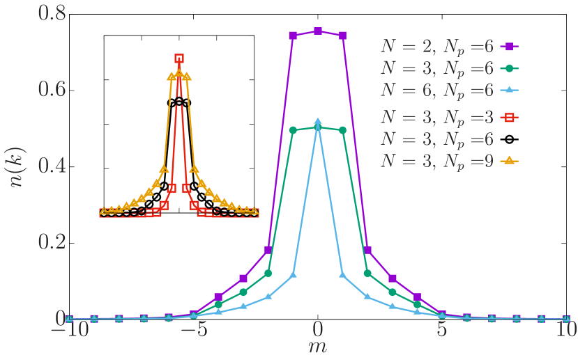
With the states obtained as summarized above, we evaluate the momentum distribution in Eq. (7). In Fig. 3, the momentum distribution in the absence of magnetic flux is presented for different SU(). For a fixed and increasing , the momentum distribution is observed to be less broad and to be more centralized around . This is to be expected since as , SU() fermions emulate bosons in terms of level occupations Pagano et al. (2014); Decamp et al. (2016). Conversely, for fixed and increasing , the momentum distribution reflects the fermionic statistics of the system, as it becomes broader due to the occupation of different momenta (see inset of Fig. 3).
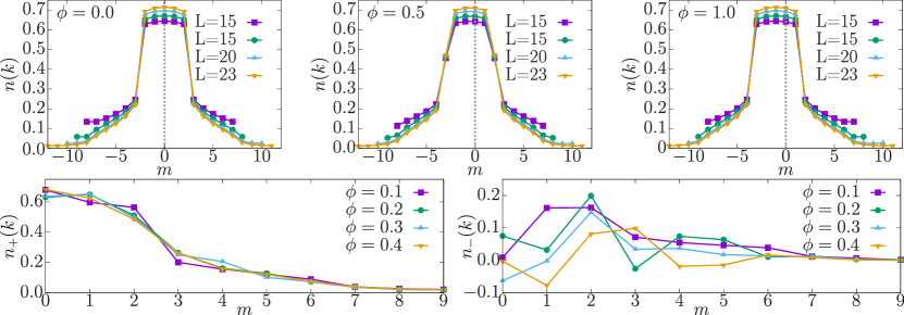
Fig. 4 depicts the momentum distribution for an SU(2) symmetric system in the presence of an effective flux. In this case, the ground-state of the Hubbard model is characterized by level crossings to counteract the flux imparted to the system Yu and Fowler (1992); Chetcuti et al. (2022b). Such level crossings correspond to different Heisenberg states, which can be obtained with the previously mentioned procedure in Sec. II by an appropriate change in spin quantum numbers (see Appendix VI.3.1). From the top row of Fig. 4, it is clear that the effect of the magnetic flux manifests itself as a shift in the momentum distribution: shift gets progressively larger with increasing flux. To capture how this happens precisely in the momentum distribution, we plot the symmetric and anti-symmetric components of the momentum distribution denoted as and respectively in the bottom panel of Fig. 4.
III.1 The Fermi gap for
In the thermodynamic limit at temperature and , the Fermi function drops from a finite value to zero at the Fermi momentum . At finite , states with can be occupied and, compared with the case, the gap at is reduced accordingly. The Fermi gap is known as the quasi-particle weight in higher dimensions and is related to the poles of the Green function with positive imaginary parts Migdal (1957); Nave et al. (2006); Otsuka et al. (2016). For SU() symmetric particles the maximum occupation of a single -level is . Consequently, the Fermi-distribution for should become a Bose-distribution (which has no gap). Therefore, this Fermi gap must tend to zero in this limit.
Since we consider finite number of particles and system size, our system is far from the thermodynamic limit. We note that parity effects appear in for SU() fermions Chetcuti et al. (2022b). Therefore we distinguish the two cases: odd occupations ( odd) and even occupations ( even). Defining the gap for the odd occupations is straight forward: every single -level up to is occupied for . For example, in the case of SU(2), , all are fully occupied. Therefore, the gap is defined as , with , where corresponds to the Fermi-distribution function. The situation is different for an even occupation per species. In this case, the levels are only partially filled and this is visible even for and finite number of particles, where a single level appears within the gap. However, this single momentum state does not enter the definition of the Fermi gap. Therefore, we define the gap in this case as . Note that in one dimension the Fermi-distribution function in the thermodynamic limit becomes a weak singularity for the Luttinger liquid Fradkin (2013). In our case, we cannot distinguish a gap from a weak singularity as we are far away from the thermodynamic limit.
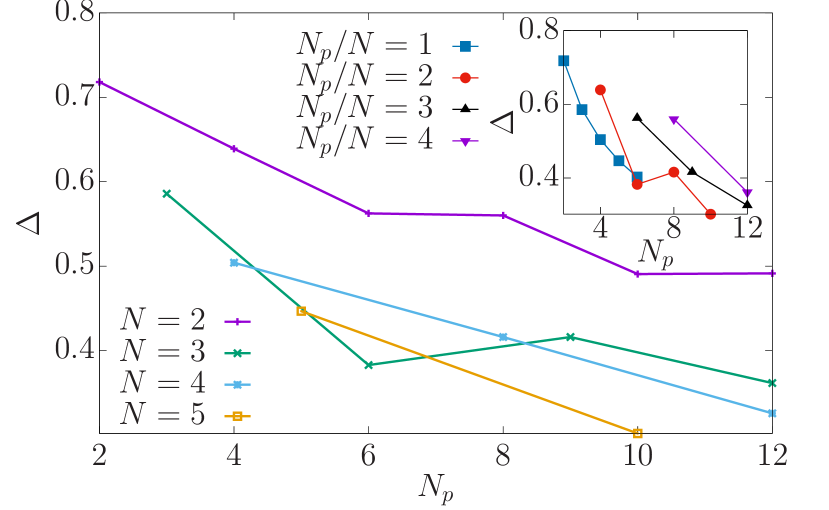
In agreement with the above argument, we find that the gap is generically going down with , but with a non-trivial dependence on and with parity effects for SU(2) and more pronounced for SU(3) - see Fig. 5. Specifically, we note that the two particles per species in the SU() symmetric case has a non-monotonous behavior with respect to the trend of decreasing gap with growing , that is present for the other curves. This behavior might be attributed to parity effects but larger systems, not attainable with current techniques, would be needed to investigate such behavior. Additionally, grouping the different gaps as a function of does not lead to strictly decreasing behavior (see inset of Fig. 5). However, we note that expecting the gap to decrease for fixed with growing , would give a hint towards a parity effect of the number of components , at least in the case . In principle, the Fermi gap need not follow a monotonic behavior. The expectation is that for each it has to eventually converge to zero as , corresponding to bosonic behaviour as mentioned previously. Lastly, it is important to notice that in the systems considered in this paper, we never come below the ratio of because we fixed the occupation of each component being the same.
IV Interference dynamics in ultracold atoms
In this section, we present a particular scenario in which the exact one-body density matrix can be tested in current state-of-the-art experimental observables in ultracold atom settings. Specifically, we consider homodyne Cai et al. (2022) and self-heterodyne Del Pace et al. (2022) protocols following the recent experiments carried out in fermionic rings.
The homodyne protocol consists in performing time-of-flight (TOF) imaging of the spatial density distribution of the atomic cloud: upon sudden release from its confinement potential, the atomic cloud expands freely, with the initially trapped atoms interfering with each other creating specific interference patterns. The resulting inteference pattern depends on the correlations that the particles have at the moment in which atomes are released. The TOF image can be calculated as
| (10) |
where is the Fourier transform of the Wannier function, denotes the position of the lattice sites in the ring in the plane and are their corresponding Fourier momenta. Note that we have taken the zeroth order of through the harmonic approximation.
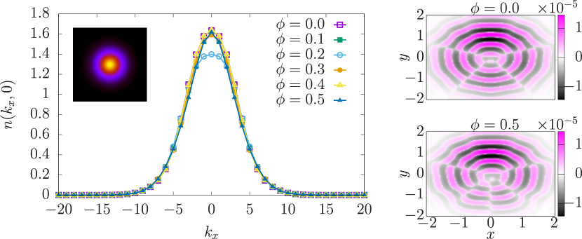
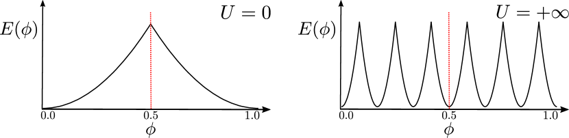
The self-heterodyne protocol follows the same procedure as the homodyne one, albeit with an additional condensate placed in the center of the system of interest, to act as a phase reference. Accordingly, as the center and the ring undergo free co-expansion in TOF, characteristic spirals emerge as the two systems interfere with each other and current is present in the system. In order to observe the phase patterns in a second quantized setting, one needs to consider density-density correlators between the center and the ring Haug et al. (2018); Chetcuti et al. (2022a): where . By exploiting the correlation matrix we calculated in the previous sections, we obtain the interference images that are obtained through the two above sketched expansion protocols for two-component fermions exactly - see Fig. 6. The left panel displays a cut on the TOF momentum distribution (at ), with the inset depicting the same quantity in the - plane. The right panels of Fig. 6 show the self-heterodyne interference pattern at zero and half flux quantum. These display the characteristic dislocations (radially segmenting lines) that at strong interactions were shown to depend on particle number, number of components and flux Chetcuti et al. (2022a). On going to the limit of infinite repulsion, the energy and consequently the persistent current landscape, changes from being periodic with the bare flux quantum to displaying a reduced periodicity of irrespective of the SU() symmetry of the system (see Fig. 7 in the Appendix). As such, the ground-state energy goes from being a single parabola at zero interaction, to having parabolic segments, that in the Bethe ansatz language are characterized by different spin quantum numbers. Remarkably, these different parabolas manifest as a result of different energy level crossings to counteract the flux threading the system, resulting in an effective fractionalization of the current. In Chetcuti et al. (2022a) it was discussed how this fractionalization can not only be monitored but also visualized in self-heterodyne interferograms, which exhibits a different number and orientation of the dislocations for the different parabolas. In the left panel of Fig. 6, we see that such dislocations are captured by our proposed scheme giving us access to the infinite repulsive limit in an exact way.
V Conclusions and Outlook
In this paper, we develop a theoretical framework to calculate the exact one-particle density matrix of -components fermions in the limit of strong repulsion using a Bethe ansatz analysis working in the integrable regime of the SU() Hubbard model. By splitting the problem into the spinless fermionic and SU() Heisenberg models, we manage to compute these observables for a number of particles , system size and number of components well beyond the current state-of-the-art tractable by numerical methods: On one hand, the numbers of particles and system size are well beyond exact diagonalization schemes; on the other hand, we remark that by Bethe ansatz we could access the limit of infinite repulsion that is a notoriously challenging limit for DMRG. On the technical side, we note that our Bethe ansatz scheme agrees well with the numerics (at least in the numbers which can be worked out) of the lattice model, also slightly beyond the dilute regime of Eq. (1). Specifically, we are able to calculate the correlations of systems composed of 38 sites and 12 particles for and , with a total configuration space of 2 billion in the spinless configuration. Depending on , this would correspond to a larger Hilbert space in the Hubbard model, such as for . Exact diagonalization/Lanczos can only handle around 7 million. Therefore, there is no direct comparison between the two methods possible in this respect.
The Fourier transform of the correlation matrix is the momentum distribution of the system. Despite being one of the simplest interesting correlation function, reflects the many-body character of the quantum state. In particular, we quantify exactly the dependence of the gap at the Fermi point on different particle numbers and number of fermion components. We confirm the general expectation that for large number of components the Pauli exclusion principle relaxes. However, we find that the suppression of the gap for finite systems is non-monotonous.
We apply this scheme to the case in which SU() matter can flow in ring-shaped potentials pierced by an effective magnetic flux . As such, an additional complication in the calculation arises since the matter-wave states obey a complex dependence on , ultimately leading to persistent currents with fractional quantization Yu and Fowler (1992); Chetcuti et al. (2022b). In particular, we read-out such phenomenon in terms of spin-states of the Heisenberg SU() model.
In this context, we give an example where the developed theory allows us to calculate readily available experimental observables such as time-of-flight measurements, both homodyne and self-heterodyne Cai et al. (2022); Del Pace et al. (2022).
We believe that our exact results can be exploited to benchmark the observables related to the one-body density matrix of SU() fermions in the strongly interacting limiting. Finally, the theoretical framework we developed opens the possibility to study more complicated correlation functions.
References
- Gogolin et al. (2004) A. O. Gogolin, A. A. Nersesyan, and A. M. Tsvelik, Bosonization and strongly correlated systems (Cambridge university press, 2004).
- Haldane (1981) F. D. M. Haldane, Journal of Physics C: Solid State Physics 14, 2585 (1981).
- Giamarchi (2003) T. Giamarchi, Quantum Physics in One Dimension (Oxford University Press, 2003).
- Takahashi (1999) M. Takahashi, Thermodynamics of One-Dimensional Solvable Models (Cambridge University Press, 1999).
- Affleck (1989) I. Affleck, Journal of Physics: Condensed Matter 1, 3047 (1989).
- Datta (1997) S. Datta, Electronic transport in mesoscopic systems (Cambridge university press, 1997).
- Fazio and Van Der Zant (2001) R. Fazio and H. Van Der Zant, Physics Reports 355, 235 (2001).
- Baeriswyl et al. (1992) D. Baeriswyl, D. K. Campbell, and S. Mazumdar, Conjugated conducting polymers , 7 (1992).
- Dresselhaus et al. (1995) M. Dresselhaus, G. Dresselhaus, and R. Saito, Carbon 33, 883 (1995).
- Cage et al. (2012) M. E. Cage, K. Klitzing, A. Chang, F. Duncan, M. Haldane, R. B. Laughlin, A. Pruisken, and D. Thouless, The quantum Hall effect (Springer Science & Business Media, 2012).
- Hewson (1997) A. C. Hewson, The Kondo problem to heavy fermions, 2 (Cambridge university press, 1997).
- Kugel et al. (2015) K. I. Kugel, D. I. Khomskii, A. O. Sboychakov, and S. V. Streltsov, Physical Review B 91, 155125 (2015).
- Arovas et al. (1999) D. P. Arovas, A. Karlhede, and D. Lilliehöök, Physical Review B 59, 13147 (1999).
- Nomura and MacDonald (2006) K. Nomura and A. H. MacDonald, Physical Review Letters 96, 256602 (2006).
- Keller et al. (2013) A. J. Keller, S. Amasha, I. Weymann, C. P. Moca, I. G. Rau, J. A. Katine, H. Shtrikman, G. Zaránd, and D. Goldhaber-Gordon, Nature Physics 10, 145 (2013).
- Scazza et al. (2014) F. Scazza, C. Hofrichter, M. Höfer, P. C. De Groot, I. Bloch, and S. Fölling, Nature Physics 10, 779 (2014).
- Hofrichter et al. (2016) C. Hofrichter, L. Riegger, F. Scazza, M. Höfer, D. R. Fernandes, I. Bloch, and S. Fölling, Physical Review X 6, 021030 (2016).
- Cappellini et al. (2014) G. Cappellini, M. Mancini, G. Pagano, P. Lombardi, L. Livi, M. Siciliani de Cumis, P. Cancio, M. Pizzocaro, D. Calonico, F. Levi, C. Sias, J. Catani, M. Inguscio, and L. Fallani, Physical Review Letters 113, 120402 (2014).
- Sonderhouse et al. (2020) L. Sonderhouse, C. Sanner, R. B. Hutson, A. Goban, T. Bilitewski, L. Yan, W. R. Milner, A. M. Rey, and J. Ye, Nature Physics 16, 1216 (2020).
- Gorshkov et al. (2010) A. V. Gorshkov, M. Hermele, V. Gurarie, C. Xu, P. S. Julienne, J. Ye, P. Zoller, E. Demler, M. D. Lukin, and A. M. Rey, Nature Physics 6, 289 (2010).
- Cazalilla and Rey (2014) M. A. Cazalilla and A. M. Rey, Reports on Progress in Physics 77, 124401 (2014).
- Capponi et al. (2016) S. Capponi, P. Lecheminant, and K. Totsuka, Annals of Physics 367, 50 (2016).
- Ludlow et al. (2015) A. D. Ludlow, M. M. Boyd, J. Ye, E. Peik, and P. O. Schmidt, Reviews of Modern Physics 87, 637 (2015).
- Marti et al. (2018) G. E. Marti, R. B. Hutson, A. Goban, S. L. Campbell, N. Poli, and J. Ye, Physical Review Letters 120, 103201 (2018).
- Livi et al. (2016) L. F. Livi, G. Cappellini, M. Diem, L. Franchi, C. Clivati, M. Frittelli, F. Levi, D. Calonico, J. Catani, M. Inguscio, and L. Fallani, Physical Review Letters 117, 220401 (2016).
- Kolkowitz et al. (2016) S. Kolkowitz, S. L. Bromley, T. Bothwell, M. L. Wall, G. E. Marti, A. P. Koller, X. Zhang, A. M. Rey, and J. Ye, Nature 542, 66 (2016).
- Rapp et al. (2007) A. Rapp, G. Zaránd, C. Honerkamp, and W. Hofstetter, Physical Review Letters 98, 160405 (2007).
- Chetcuti et al. (2021) W. J. Chetcuti, J. Polo, A. Osterloh, P. Castorina, and L. Amico, “Probe for bound states of su(3) fermions and colour deconfinement,” (2021).
- Amico and Korepin (2004) L. Amico and V. Korepin, Annals of Physics 314, 496 (2004).
- Yang (1967) C. N. Yang, Physical Review Letters 19, 1312 (1967).
- Sutherland (1968) B. Sutherland, Physical Review Letters 20, 98 (1968).
- Fradkin (2013) E. Fradkin, Field theories of condensed matter physics (Cambridge University Press, 2013).
- Ogata and Shiba (1990) M. Ogata and H. Shiba, Physical Review B 41, 2326 (1990).
- Roth and Burnett (2003) R. Roth and K. Burnett, Physical Review A 67, 031602 (2003).
- Amico et al. (2005) L. Amico, A. Osterloh, and F. Cataliotti, Physical Review Letters 95, 063201 (2005).
- Amico et al. (2022) L. Amico, D. Anderson, M. Boshier, J.-P. Brantut, L.-C. Kwek, A. Minguzzi, and W. von Klitzing, Reviews of Modern Physics 94, 041001 (2022).
- Chetcuti et al. (2022a) W. J. Chetcuti, A. Osterloh, L. Amico, and J. Polo, “Interference dynamics of matter-waves of su() fermions,” (2022a).
- Decamp et al. (2016) J. Decamp, J. Jünemann, M. Albert, M. Rizzi, A. Minguzzi, and P. Vignolo, Physical Review A 94, 053614 (2016).
- Cai et al. (2022) Y. Cai, D. G. Allman, P. Sabharwal, and K. C. Wright, Physical Review Letters 128, 150401 (2022).
- Del Pace et al. (2022) G. Del Pace, K. Xhani, A. Muzi Falconi, M. Fedrizzi, N. Grani, D. Hernandez Rajkov, M. Inguscio, F. Scazza, W. J. Kwon, and G. Roati, Physical Review X 12, 041037 (2022).
- Yu and Fowler (1992) N. Yu and M. Fowler, Physical Review B 45, 11795 (1992).
- Chetcuti et al. (2022b) W. J. Chetcuti, T. Haug, L.-C. Kwek, and L. Amico, SciPost Physics 12, 33 (2022b).
- Dalibard et al. (2011) J. Dalibard, F. Gerbier, G. Juzeliūnas, and P. Öhberg, Reviews of Modern Physics 83, 1523 (2011).
- Lieb and Wu (1968) E. H. Lieb and F. Y. Wu, Phys. Rev. Lett. 20, 1445 (1968).
- Takahashi (1970) M. Takahashi, Progress of Theoretical Physics 44, 899 (1970).
- Korepin et al. (1997) V. E. Korepin, N. M. Bogoliubov, and A. G. Izergin, Quantum inverse scattering method and correlation functions, Vol. 3 (Cambridge university press, 1997).
- Essler et al. (2005) F. H. Essler, H. Frahm, F. Göhmann, A. Klümper, and V. E. Korepin, The one-dimensional Hubbard model (Cambridge University Press, 2005).
- Caux (2009) J.-S. Caux, Journal of mathematical physics 50, 095214 (2009).
- Sutherland (1975) B. Sutherland, Physical Review B 12, 3795 (1975).
- Note (1) It is worth noticing that this eigenvalue may be accidentally degenerate in the Heisenberg model.
- Frahm and Schadschneider (1995) H. Frahm and A. Schadschneider, “On the bethe ansatz soluble degenerate hubbard model,” in The Hubbard Model: Its Physics and Mathematical Physics (Springer US, Boston, MA, 1995) pp. 21–28.
- White (1992) S. R. White, Physical Review Letters 69, 2863 (1992).
- Fishman et al. (2022) M. Fishman, S. R. White, and E. M. Stoudenmire, SciPost Phys. Codebases , 4 (2022).
- Pagano et al. (2014) G. Pagano, M. Mancini, G. Cappellini, P. Lombardi, F. Schäfer, H. Hu, X.-J. Liu, J. Catani, C. Sias, M. Inguscio, and L. Fallani, Nature Physics 10, 198 (2014).
- Migdal (1957) A. B. Migdal, JETP 32, 399 (1957).
- Nave et al. (2006) C. P. Nave, D. A. Ivanov, and P. A. Lee, Physical Review B 73, 104502 (2006).
- Otsuka et al. (2016) Y. Otsuka, S. Yunoki, and S. Sorella, Physical Review X 6, 011029 (2016).
- Haug et al. (2018) T. Haug, J. Tan, M. Theng, R. Dumke, L.-C. Kwek, and L. Amico, Physical Review A 97, 013633 (2018).
- Cornwell (1997) J. F. Cornwell, Group Theory in Physics: An Introduction (Academic Press, 1997).
- Pfeifer (2003) W. Pfeifer, The Lie Algebras su(N): An Introduction (Birkhäuser, 2003).
- Georgi (1999) H. Georgi, Lie Algebras in Particle Physics (Westview Press, 1999).
VI Appendix
In the following sections, we provide supporting details of the theory discussed in the manuscript.
VI.1 Separation of the spin and charge degrees of freedom
The one-dimensional SU(2) Hubbard Hamiltonian describing particles with flipped spins residing on a ring-shaped lattice with sites,
| (1) |
which is Bethe ansatz integrable. It was found that the eigenfunctions of the Hubbard model within a given sector are of the form
| (2) |
where and are permutations introduced to account for the eigenstates’ dependence on the respective ordering of the fermion coordinates and quasimomenta , with being the spin-dependent amplitude. The spin wavefunction contains all the spin configurations of the down spins can be expressed as
| (3) |
whereby we define
| (4) |
with corresponding to the coordinate of the electrons with spin-down in a given sector . As , we can neglect the terms such that
| (5) |
After this treatment, the spin wavefunction is no longer dependent on the charge degrees of freedom through . Consequently, the Bethe ansatz wavefunction as can be recast into the following form
| (6) |
Additionally, we can go a step forward and show that in this limit the spin wavefunction corresponds to that of the one-dimensional anti-ferromagnetic SU(2) XXX Heisenberg chain. Indeed, it can be shown that
| (7) |
by defining and . Consequently, the spin wavefunction becomes
| (8) |
which except for a phase factor corresponds to the Bethe ansatz wavefunction of the Heisenberg model. Therefore, we have that
| (9) |
The same treatment can be applied for the SU() Hubbard model, which results to be integrable in two limits: (i) large repulsive interactions and filling fractions of one particle per site Sutherland (1975); (ii) in the continuum limit of vanishing lattice spacing achievable by dilute filling fractions Sutherland (1968); Capponi et al. (2016). The Bethe ansatz wavefunction for the model is of the same form as the one outlined in Equation (2) with the added difference that the houses the extra spin degrees of freedom. In the following, we will focus on the second integrable regime and illustrate the decoupling of the spin and charge degrees of freedom for SU() fermions through the Bethe ansatz equations.
VI.1.1 Extension to SU(N) fermions
In the continuous limit, the SU() Hubbard model tends to the Gaudin-Yang-Sutherland Hamiltonian describing -component fermions with a delta potential interaction Sutherland (1968); Decamp et al. (2016), which reads
| (10) |
where is the number of fermions with colour of with , being the size of the ring and denoting the effective magnetic flux threading the system.
The Bethe ansatz equations for the model are as follows,
| (11) |
| (12) |
for where , and . denotes the number of particles, corresponds to the colour with and being the charge and spin momenta respectively. The energy corresponding to the state for every solution of these equations is .
For SU(3) fermions, one obtains the three nested non-linear equations
| (13) |
| (14) |
| (15) |
where and were changed to and for the sake of convenience. In the limit Ogata and Shiba (1990); Yu and Fowler (1992); Chetcuti et al. (2022b) we observe that will tend to zero, since all of the ground-state are real here for repulsive . Consequently, the Bethe equations read
| (16) |
| (17) |
| (18) |
defining and respectively. The Bethe equations decouple into that of a model of spinless fermions (16) and those of an SU(3) Heisenberg magnet (17) and (18).
Subsequently, by taking the logarithm of Equations (16) through (18) and using
| (19) |
it can be shown that the quasimomenta can be expressed as Chetcuti et al. (2022b)
| (20) |
in terms of the charge and two sets of spin , quantum numbers. By exploiting different configurations of these quantum numbers, we can construct all the excitations and the corresponding Bethe ansatz wavefunction. The procedure outlined here holds for any -component fermionic systems, with the added difference that there will be sets of spin quantum numbers (2 for the considered SU(3) case).
For strong repulsive couplings, the ground-state energy of the Hubbard model fractionalizes with a reduced period of as a combined effect of the effective magnetic flux, interaction strength and spin correlations Yu and Fowler (1992); Chetcuti et al. (2022b), which is in turn reflected in the momentum distribution Chetcuti et al. (2022a). In the Bethe ansatz language, this phenomenon is accounted for through various configurations of the spin quantum numbers that correspond to different spin excitations that are generated in the ground-state to counteract the increase in the flux.
VI.2 SU(N) Heisenberg model
The SU(2) Heisenberg model is a sum of permutation operators
| (21) |
with corresponding to the Pauli matrices, the three generators of the SU Lie algebra. In the case of the SU() Heisenberg model, the Hamiltonian can be constructed in a similar fashion Sutherland (1975); Capponi et al. (2016). In general we obtain for the generators of the SU()
| (22) |
which acts on sites and permuting the SU() states.
VI.2.1 Details about the SU(N) Generators
The generators in the Lie algebra of SU() are analogues of the Pauli matrices in SU(2). Taking SU(3) as an example, we have six non-diagonal generators
| (23) |
that together with two diagonal generators
| (24) |
comprise the Gell-Mann matrices that are the matrix representation of the SU(3) Lie algebra. For generalization purposes, the generators were grouped by defining , which are analogues to the that operate between the different subspaces of SU(3) which are , . Here, both run from 1 to . We decided to group the elements of the diagonal Cartan basis at the end as and ,
which differs from the standard Gell-Mann matrices, but is eases the generalisation. For the extension to , one has to consider the elements , which would correspond to in some space , where . Additionally, the corresponding diagonal Cartan elements need to be taken into account. There are Cartan elements that can be constructed via the following formula where ; the occurs times, respectively.
VI.2.2 Casimirs of SU(N) fermions
Whereas in SU(2) we have a single Casimir operator, for SU() we are faced with Casimirs. Out of these Casimirs, we are only interested in the quadratic Casimir, which for the fundamental representation reads
| (25) |
as it relates to the total spin quantum number , which is necessary for us to classify the Heisenberg eigenstates.
To this end we have to evaluate
the Casimir in various SU() representations. In the following, we sketch
the procedure to write the quadratic Casimir operator for SU(3) and SU(4).
We start by looking at the SU(3) case, where its representations are labeled by integer numbers which correspond to the simple Cartan elements : . The elements are given by
| (26) |
| (27) |
To calculate the quadratic Casimir values for these representations , we need the Cartan matrix
| (28) |
defined using the Killing form (see Cornwell (1997), chapter 12 for the evaluation of the Casimir). We obtain
| (29) |
giving the value of for the fundamental representations and . Here, (see Cornwell (1997); Pfeifer (2003); Georgi (1999)) for the positive roots . These are the two simple roots together with their sum, . If one introduces half-integer values as in the SU(2) representation for each such that (), we obtain
| (30) |
Likewise for SU(4), the representations of SU(4) are labeled by the Cartan elements : , which are given by
| (31) |
| (32) |
| (33) |
The corresponding Cartan matrix reads
| (34) |
Upon evaluating the quadratic Casimir as in Equation (30), we have that
| (35) |
with . Here, the positive roots are the three simple roots together with , , and . Introducing half-integer values as for SU(2), we obtain
| (36) |
leading to the value of for the fundamental representations and , and for the representation .
VI.3 Evaluating Correlation functions
In the previous sections, we outlined how the spin and charge degrees of freedom decouple yielding a simplified form of the Bethe ansatz wavefunction (37), that at infinite repulsion reads
| (37) |
Here, we are going to show how to evaluate the Slater determinant of the charge degrees of freedom and the corresponding spin wavefunction in the presence of an effective magnetic flux.
VI.3.1 Slater determinant
To calculate the Slater determinant of spinless fermions, we need to start by noting that
| (38) |
where , denotes the sum over the spin quantum numbers and is the angular momentum. is a constant shift can be or for systems with and fermions respectively, that will henceforth be termed as paramagnetic and diamagnetic. Through Equation (38), we can re-write the Slater determinant in the following form
| (39) |
with denoting which we refer to as the center of mass. The matrix elements of the determinant are of the form , whereby we made use of the fact that all the quasimomenta are equidistant. By noting that the matrix in Equation (39) has the same structure of the Vandermonde matrix Ogata and Shiba (1990), we can express the Slater determinant as
| (40) |
which upon simplification reads
| (41) |
This expression can be further simplified by noticing that
| (42) |
that in conjunction with Equation (38) reduces Equation (40) into
| (43) |
In the presence of an effective magnetic flux, the variables and need to be changed in order to counteract the increase in flux. For the spin quantum numbers, the shift needs to satisfy the degeneracy point equation Yu and Fowler (1992); Chetcuti et al. (2022b)
| (44) |
with ranging from 0.0 to 1.0 and being 0 [] for diamagnetic [paramagnetic] systems. Upon increasing , the angular momentum of the system increases at with being (half-odd) integer in the case of (diamagnetic) paramagnetic systems, with for an odd number of particles.
VI.3.2 Resolving degeneracies of the spin wavefunction
As , all the spin configurations of the model are degenerate. The reason is that the energy contribution from the spin part of the wavefunction is of the order . However, there is no spin degeneracy observed in the Hubbard model; the ground-state is non-degenerate for SU(), except for special points in flux with an eigenenergy crossing. Hence, a single state has to be chosen properly for matching with the Hubbard model. Due to the symmetry of both models, we choose the square of the total spin, , or quadratic Casimir operator to label the eigenstates.
The selected eigenstates of both models need to have the same value for this operator. We used this benchmarking with the Hubbard model only
for small system sizes in order to understand what are the
representations of the Heisenberg model we have to choose.
We observe that the resulting composition from spinless Fermions and Heisenberg Hamiltonian results in a translationally invariant model only in cases where these states match. We use this as a control mechanism.
As already explained in the main text, the spin wavefunction is obtained by performing exact diagonalization resp. Lanczos methods of the one-dimensional anti-ferromagnetic Heisenberg model.
a) Zero flux – The ground-state with odd and even number of particles per species for the Hubbard model corresponds to different values of the Casimir operator, and therefore to different representations of the SU() algebra. For odd number of particles per species , it corresponds to a singlet state for all SU().
The ground-state of the anti-ferromagnetic Heisenberg model instead is always a singlet
and non-degenerate for all SU().
Therefore, we choose this state as the lowest energy eigenstate of the Heisenberg model with this property for
for an odd occupation number per species.
For an even number of particles per species, we have to choose a different state.
For the SU(2) this is the lowest non-degenerate excited triplet-state (of total spin , ) in the spectrum of the Heisenberg model. It corresponds to an -representation (see section VI.2.2 of the Appendix). For SU(), i.e. and , it is the first non-degenerate state with Casimir eigenvalue .
Examples are the -dimensional representations for SU(3)
and correspondingly
for SU(4). The numbers in the SU(3) representations correspond to the numbers and frequently used in SU(3) representations in the mathematical literature or high energy physics; there they represent the number of (anti-)quarks. The dimension of a representation of SU(3) is .
Both representations for SU(3) and SU(4)
have a Casimir value of .
We assume that this representation will be for SU().
This state takes the role of the non-degenerate triplet state of SU(2)
in the zero field ground-state for an even species number occupation.
b) Non-zero flux– The analysis of non-zero magnetic flux is motivated from an atomtronics context Chetcuti et al. (2021, 2022a). As mentioned previously, for strong repulsive interactions a fractionalization of the persistent currents in the model is observed Yu and Fowler (1992); Chetcuti et al. (2022b). Figure 7 shows an example of the change of the energy landscape when going from non-interacting to strongly interacting particles in presence of an effective magnetic flux. This fractionalization appears since formerly higher excited states are bent by the field to be the ground-state. A unique method to identify these states would be to utilize the SU() Heisenberg Bethe equations, which need to have the same spin quantum number configurations as their Hubbard counterparts. In this manner, we are guaranteed that the corresponding eigenstates obtained from the Heisenberg model correspond to the ground-state of the Hubbard model. However, it is rather tedious to achieve the whole state using this method. This is particularly true because the Bethe ansatz gives direct solutions only for the highest weight states and we work at an equal occupation of each species: the resulting state is then obtained by applying sufficiently often the proper lowering operators of SU().
In the case of paramagnetic systems, i.e. an even number of particles per species, the central fractionalized parabola (centered around ), corresponds to a singlet state. This parabola results to be non-degenerate for the Heisenberg model and is therefore easily distinguished. As such,
one obtains the corresponding states for the outer and central fractionalized parabolas in a straight forward manner for arbitrary SU().
We mention though that in order to find the
corresponding state for the outer parabola and the
paramagnetic case (even occupation of each species),
we have to single out a non-degenerate excited state with Casimir value .
For finite field and degenerate ground-states of the Hubbard model, we do not have a general procedure to choose the states for SU(). Therefore, we explain our approach in
considering SU(2) first and then apply it to
SU(3) symmetric fermions.
In the case of SU(2), the remaining fractionalized parabolas (i.e. excluding the two outer parabolas and the central one) have a common spin value of . This in turn results in a two-fold degeneracy in the spin- Heisenberg model for a given collective spin quantum number . Hence, the relevant states for two of the parabolas of a given are superpositions of these degenerate eigenstates of the Heisenberg Hamiltonian. These states can be separated by different eigenvalues for , part of the Heisenberg model but not commuting with it. We call both eigenstates of this permutation operator . The states corresponding to the inner branches of the fractionalization are obtained from the two spin- and energy-degenerate states as
| (45) |
It is worth mentioning that these states correspond to fractionalized parabolas that emerge from a singlet state in the absence of flux to a non-degenerate triplet state with each of the basis elements being non-zero.
This happens here gradually via intermediate triplet states where certain basis states are excluded. As an example, we take an SU(2) state with particles to explain this better. Since this state has particles of each species ( or ) the parabolas start from a singlet and persist as a triplet state during their fractionalization up to the center parabola.
The singlet state is made of three distinct configurations: a) , b) , and c) the possible remaining configurations with alternating sign (singlet state). This is mediated via fractionalized states where the component a) is missing in the first inner parabola and additionally the component b) vanishes for the second parabola. The triplet of the central parabola has the same components as the singlet state but without alternating signs.
For SU(2) the corresponding states that belong to the fractionalized parabolas have been triplet states, as was the non-degenerate state corresponding to either the central (diamagnetic, odd species number) or the outer parabola (paramagnetic, even species number). However, the representations are modified for in the intermediate parabolas. In the case of SU(3) we obtain as the -dimensional representation (instead of ) which governs the intermediate parabola. For SU(4) it is instead of (see Appendix VI.2.2).
The Casimir has values and respectively.
These representations take the role of the
degenerate triplet state of SU(2).
In the case non-vanishing flux threading a ring of SU symmetric fermions, the ground-states of the Hubbard Hamiltonian (1) belonging to a given , is -fold degenerate coming from the sets of spin quantum numbers. This degeneracy holds for the inner fractionalized parabolas. As a consequence of its one-to-one correspondence with the Hubbard model, these degeneracies are manifested in the Heisenberg model, in addition to the two-fold degeneracy mentioned previously for both parabolas with equal values for . In order for this extra degeneracy to be resolved, we make certain coefficients of the wavefunction in the Heisenberg basis vanish by according superpositions of the degenerate states. This has been motivated by former observations in SU(2) (see discussion above).
To get a better idea of how this is done explicitly, here we exemplify on the case of 3 particles in SU(3). There are only two possible values for in this case and each parabola is two-fold degenerate in the Hubbard model. The degeneracy of the Heisenberg model is hence 4-fold. So, the distinct states have to be selected from a remaining two-fold degeneracy of the operator . The zeroth parabola is in the singlet state of SU(3) that belongs to for which every component of the wavefunction is non-zero. Both two-fold degenerate inner parabolas have and correspond in one case to the positive or negative permutation of the species number only; in the second degenerate case they correspond to configurations and as the only non-zero component. These are the states that are to be superposed by formula (45). The direct way to obtain the corresponding state of the Heisenberg model is via the Bethe ansatz wavefunction for the same spin quantum numbers of the Hubbard model. The degeneracies amount to -fold for the SU() Heisenberg model. These are distinguished by the eigenstates of the permutation operator up to a remaining -fold degeneracy.
VI.4 Comparison with numerics
In this section, we compare the correlations obtained via the method presented in this paper to those obtained through exact diagonalization using the Lanczos algorithm. The error between the two methods is estimated by calculating the relative correlation distance for the ground state, which is defined as
| (46) |
where correspond to the correlations obtained through exact diagonalization. We note that because of the periodicity of the system all are a circular shift of , such that we only need to sum once. Some of the comparisons that were carried out are tabulated in Table 1. Naturally, we find that as one goes to large interactions, the agreement of the correlations between the two methods increases. Such a result is to be expected as our proposed scheme is viable in the limit of infinite repulsion. Furthermore, we highlight that our system is far from being in the dilute limit, which is one of the integrable regimes of the Hubbard model. In spite of this, there is an excellent agreement between exact diagonalization and our scheme that is intrisically reliant on the system being Bethe ansatz integrable. Bethe ansatz integrability hinges on the fact that the scattering of more than two particles does not occur (Yang-Baxter factorization of the scattering matrix). In the infinite repulsive regime, the multiparticle scattering is suppressed since the probability of two particles interacting is vanishing. Therefore, despite the fact that we are far from the dilute limit condition, the system is indeed very close to be integrable for low lying states, and our method is able to accurately tackle the infinite repulsive limit of the SU() Hubbard model.
| 15 | 4 | 2 | 750 | |
| 15 | 4 | 2 | 10,000 | |
| 15 | 6 | 2 | 750 | |
| 15 | 6 | 2 | 5000 | |
| 15 | 3 | 3 | 1000 | |
| 15 | 3 | 3 | 5000 | |
| 10 | 6 | 3 | 1000 | |
| 10 | 6 | 3 | 5000 |
The Hilbert space of the Hubbard model for an equal number of particles per colour is given by , where corresponds to the system size, to the number of particles in a given colour, and is the number of components. It is straightforward to see that the size of the Hilbert space increases at least exponentially on going to a larger value of any of these three variables. When it comes to exact diagonalization, the size of the Hilbert space is one of the limitations as it exceeds the memory of the computer defined as Msize. This can be estimated in the following manner , where we count the number of configurations, the number of particles (that gives the numbers we need to store) and the bits occupy by Int64, then we convert this into GigaBytes. Specifically, through our scheme we are able to consider systems with , and , which correspond to a Msize GB for the spinless, and 3500 TB for the corresponding Hubbard model, which is clearly not attainable in current High Performance Computing systems. However, in our case we can perform calculations without storing the configurations. Similar approaches can also be followed in exact diagonalization, but not with these parameters.
In the current state-of-the-art, one can diagonalize a Hilbert space of around 7 million (corresponding to Msize=GB) using the Lanczos algorithm
when taking into account the large matrices and values of the interactions used in the numerical operations, such as for example the calculation of correlations. Our proposed scheme is able to go to larger system parameters on account of the spin-charge decoupling.
By separating the problem into the spinless and Heisenberg parts, we deal with small Hilbert space dimensions that are given by and respectively. In doing so, the size of the system that we can consider, i.e. the number of sites, comes down to calculating the Slater determinant (43). Such a calculation is limited not by the memory size but by its runtime. However, in this manner one can calculate large system sizes, such as for example 38 sites that corresponds to a Hilbert space of around 2 billion for the spinless part. The other part of the problem lies in diagonalizing the Heisenberg matrix, whose dimensions are significantly smaller than its Hubbard counterpart, enabling us to calculate the system parameters displayed in this manuscript. It should be stressed that even through this scheme one is not able to calculate systems with very large particle numbers, as this part of the calculation is still affected by the dimensions of the matrix under consideration. Additionally, for we need to consider the excited states of the Heisenberg model in order to get the actual ground-state of the Hubbard system, which means that we need to perform the full diagonalization of the former instead of employing the lanczos algorithm.
Lastly, we close this section by drawing comparisons with DMRG. The system under consideration is infinitely repulsive SU() fermions residing on a ring. In this context, DMRG has problems with convergence due to the large repulsive interactions and the high number of degeneracies present in the system. It is also limited by the periodic boundary conditions. Nonetheless, as we remarked in the manuscript, in the regime of intermediate interactions, DMRG can still be employed giving a good agreement with exact diagonalization and the proposed scheme.