Beyond Mahalanobis-Based Scores for
Textual OOD Detection

Abstract

Deep learning methods have boosted the adoption of NLP systems in real-life applications. However, they turn out to be vulnerable to distribution shifts over time which may cause severe dysfunctions in production systems, urging practitioners to develop tools to detect out-of-distribution (OOD) samples through the lens of the neural network. In this paper, we introduce TRUSTED, a new OOD detector for classifiers based on Transformer architectures that meets operational requirements: it is unsupervised and fast to compute. The efficiency of TRUSTED relies on the fruitful idea that all hidden layers carry relevant information to detect OOD examples. Based on this, for a given input, TRUSTED consists in (i) aggregating this information and (ii) computing a similarity score by exploiting the training distribution, leveraging the powerful concept of data depth. Our extensive numerical experiments involve 51k model configurations, including various checkpoints, seeds, and datasets, and demonstrate that TRUSTED achieves state-of-the-art performances. In particular, it improves previous AUROC over 3 points.

1 Introduction

The number of AI systems put into production has steadily increased over the last few years. This is because advanced techniques of Machine Learning (ML) and Deep Learning (DL) have brought significant improvements over previous state-of-the-art (SOTA) methods in many areas such as finance [17, 57], transportation [59], and medicine [14, 77]. However, the increasing use of black-box models has raised concerns about their societal impact: privacy [33, 64, 74, 29], security [6, 3, 20], safety [41, 50, 18], fairness [5, 72], and explainability [13, 63] which became areas of active research in the ML community.

This paper is about a critical safety issue, namely Out-Of-Distribution (OOD) detection [11], which refers to a change of distribution of incoming data that may cause failures of in-production AI systems. When data are tabular and of small dimension, simple statistical methods can be efficient, and one may, for instance, monitor the mean and variance of each marginal over time. However, these traditional methods do not work anymore when data are high-dimensional and/or unstructured. Thus, the need to design new techniques that incorporate incoming data and the neural networks themselves.

Distinguishing OOD examples from in-distribution (ID) examples is challenging for modern deep neural architectures. DL models transform incoming data into latent representations from which reliable information extraction is cumbersome. Because of that, designing new tools of investigation for large pretrained models, judiciously named foundation models by [9], is an essential line of research for the years to come. In computer vision, methods are more mature thanks to the availability of appropriate deformation techniques that allow for sensitivity analysis. In contrast, the nature of tokens in Natural Language Processing (NLP) makes it more difficult to develop such suitable methods.

In this paper, we focus on classifiers for textual data and on the ubiquitous BERT [34], DistilBERT [83], and RoBERTa [68] architectures. Existing methods can be grouped according to their positioning with respect to the network. Some works exploit only the incoming data and compare them with in-distribution examples through likelihood ratios [42, 19]. Another line of research consists in incorporating robust constraints during training, with [48] or without [103, 60] access to some available OOD examples. Another line of research focuses on post-processing methods that can be used on any pretrained models. In our view, these are the most promising tools because typical users rely on transformers without retraining. Within post-processing methods, one can distinguish softmax-based tools that compute a confidence score based on the predicted probabilities and threshold to decide whether a sample is OOD or not. Notice that this does not require direct access to in-distribution data. The seminal work is due to Hendrycks [47] who uses the maximum soft-probability, and has been pushed further in [62, 52]. In [67], authors suggest looking one step deeper into the network, namely, to compute a confidence score based on the projections of the pre-softmax layer. More recently, [75] achieved SOTA results on transformer-based encoder by computing the Mahalanobis distance [71, 32] between a test sample and the in-distribution law [58], estimated through accessible training data points.

Nevertheless, the distance-based score is computed on the last-layer embedding only, suggesting that going deeper inside the network might improve OOD detection power. Moreover, the computation of Mahalanobis-based scores requires inverting the covariance matrix of the training data, which can be prohibitive in high dimensions. It is worth noticing that the Mahalanobis-based scores can be seen as a data depth [97, 104] through a simple re-scaling [66], that is a statistical function measuring the centrality of an observation with respect to a probability distribution. Although data depths are quite natural in the context of OOD detection, they remain overlooked by the ML community. In the present work, we rely on the recently introduced Integrated Rank-Weighted depth [76, 94] in order to remedy the drawbacks of the Mahalanobis-based scores for OOD detection.

1.1 Our contribution

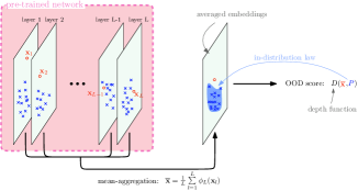
Fig. 1: TRUSTED detector. It relies on two steps: mean layer aggregation followed by the computation of $D_{\mathrm{IRW}}$.

We first leverage the observation introduced by previous work that all hidden layers of a neural network carry useful information to perform textual OOD detection. For a given input ${\bf x}$, our method consists in computing its average latent representation $\overline{{\bf x}}$ and then its OOD score through the depth score of $\overline{{\bf x}}$ with respect to the averaged in-distribution law (see Fig. 1 for an illustration). Notice that the ability to compute averaged latent representations crucially relies on the structure of transformers layers that share the same dimension. The depth function we are using is based on the computation of the projected ranks of the test inputs using randomly sampled directions. From a theoretical viewpoint, this novel method requires fewer assumptions on the data structure than the Mahalanobis score.

We conduct extensive numerical experiments on three transformers architectures and eight datasets and benchmark our method with previous approaches. To ensure reliable results, we introduce a new framework for evaluating OOD detection that considers hyperparameters that were unreported before. It consists of computing performances for various choices of checkpoints and seeds, which allows us to report a variance term that makes some previous methods fall within the same performance range. Our conclusions are drawn by considering over 51k configurations, and show that our new detector based on data depth improves SOTA methods by 3 AUROC points while having less variance. This result supports the intuition that OOD detection is a matter of looking at the information available across the entire network. Our contribution can be summarized as follows:

1. We introduce a novel OOD detection method for textual data. Our detector TRUSTED relies on the full information contained in pretrained transformers and leverages the concept of data depth: a given input is detected as being in-distribution or OOD sample based on its depth score with respect to the training distribution.

2. We conduct extensive numerical experiments and prove that our method improves over SOTA methods. Our evaluation framework is more reliable than previous studies as it includes the variance with respect to seeds and checkpoints.

3. We release open-source code and data to ease future research, ensure reproducibility and reduce computation overhead.

2 Problem Formulation

Training distribution and classifier. Let us denote by $\mathcal{X}$ the textual input space. Consider the multiclass classification setup with target space $\mathcal{Y}=\{1,\ldots,C\}$ of size $C\geq 2$. We assume the dataset under consideration is made of $N\geq 1$ i.i.d. samples $(\mathbf{x}_{1},y_{1}),\ldots,(\mathbf{x}_{N},y_{N})$ with probability law denoted by $p_{XY}$ and defined on $\mathcal{X}\times\mathcal{Y}$. Accordingly, we will denote by $p_{X}$ and $p_{Y}$ the marginal laws of $p_{XY}$. Finally, we denote by $f_{N}:\mathcal{X}\rightarrow\mathcal{Y}$ the classifier that has been trained using $(\mathbf{x}_{i},y_{i})$.

Open world setting. In real-life scenarios, the trained model $f_{N}$ is deployed into production and will certainly be faced with input data whose law is not $p_{XY}$. To each test point $(\mathbf{x},y)$, we associate a variable $z\in\{0,1\}$ such that $z=0$ if $(\mathbf{x},y)$ stems from $p_{XY}$ and $z=1$ otherwise. It is worth emphasizing that in our setting $f_{N}$ has never been faced with OOD examples before deployment. This is usually referred to as the open-world setting. From a probabilistic viewpoint, the test set distribution of the input data $p^{\mathrm{test}}_{X}$ is a mixture of in-distribution and OOD samples:

$$p^{\mathrm{test}}_{X}(\mathbf{x})=\alpha~{}p_{X|Z}(\mathbf{x}|z=1)+(1-\alpha)~{}p_{X|Z}(\mathbf{x}|z=0),$$

where $\alpha\in(0,1)$. In this work, we will not make any further assumptions on the proportion $\alpha$ of OOD samples and on the OOD pdf $p_{X|Z}(\mathbf{x}|z=1)$, making the problem more difficult but at the same time more well suited for practical use. Indeed, for textual data, it does not appear to be realistic to model how a corpus can evolve.

OOD detection. The objective of OOD detection is to construct a similarity function $s:\mathcal{X}\rightarrow\mathbb{R}_{+}$ that accounts for the similarity of any element in $\mathcal{X}$ with respect to the training in-distribution. For a given test input $\mathbf{x}$, we then classify $\mathbf{x}$ as in-distribution or OOD according to the magnitude of $s(\mathbf{x})$. Therefore, one fixes a threshold $\gamma$ and classifies IN (i.e. $\hat{z}=0$) if $s(\mathbf{x})>\gamma$ or OOD (i.e. $\hat{z}=1$) if $s(\mathbf{x})\leq\gamma$. Formally, denoting $g(\cdot,\gamma)$ the decision function, we take:

$$g(\mathbf{x},\gamma)=\left\{\begin{array}[]{ll}1&\text{if }s\left(\mathbf{x}\right)\leq\gamma,\\ 0&\text{if }s\left(\mathbf{x}\right)>\gamma.\end{array}\right.$$ (1)

Performance evaluation. The OOD problem is a (unbalanced) classification problem, and classically, two quantities allow to measure the performance of a method. The false alarm rate is the proportion of samples that are classified as OOD while they are IN. For a given threshold $\gamma$, it is theoretically given by $\Pr\big{(}s(\mathbf{X})\leq\gamma\,|\,Z=0\big{)}$. The true detection rate is the proportion of samples that are predicted OOD while being OOD. For a given threshold $\gamma$, it is theoretically given by $\Pr\big{(}s(\mathbf{X})\leq\gamma\,|\,Z=1\big{)}$.

There exist several ways to measure the effectiveness of an OOD method. We will focus on four metrics. The first two are specifically designed to assess the quality of the similarity function $s$.

Area Under the Receiver Operating Characteristic curve (AUROC) [10]. It is the area under the ROC curve $\gamma\mapsto(\Pr\big{(}s(\mathbf{X})>\gamma\,|\,Z=0\big{)},\Pr\big{(}s(\mathbf{X})\leq\gamma\,|\,Z=1\big{)})$, which plots the true detection rates against the false alarm rates. The AUROC corresponds to the probability that an in-distribution example $\mathbf{X}_{in}$ has higher score than an OOD sample $\mathbf{X}_{out}$: ${\texttt{AUROC}}=\Pr(s(\mathbf{X}_{in})>s(\mathbf{X}_{out}))$, as can be checked from elementary computations.

Area Under the Precision-Recall curve (AUPR-IN/AUPR-OUT) [31]. It is the area under the precision-recall curve $\gamma\mapsto(\Pr\big{(}Z=1\,|\,s(\mathbf{X})\leq\gamma\big{)},\Pr\big{(}s(\mathbf{X})\leq\gamma\,|\,Z=1\big{)})$ which plots the recall (true detection rate) against the precision (actual proportion of OOD amongst the predicted OOD). The AUPR is more relevant to unbalanced situations.

The third metric we will use is more operational as it computes the performance at a specific threshold $\gamma$ corresponding to a security requirement.

False Positive Rate at $95\%$ True Positive Rate (FPR). In practice, one wishes to achieve reasonable level of OOD detection. For a desired detection rate $r$, this incites to fix a threshold $\gamma_{r}$ such that the corresponding TPR equals $r$. At this threshold, one then computes:

$$\Pr(s(\mathbf{X})\geq\gamma_{r}\,|\,z=0)\quad\text{with $\,\,\gamma_{r}\,\,$ s.t. $\,\,\textrm{TPR}(\gamma_{r})=r$.}$$ (2)

In our work, we set $r=0.95$ in (2).

Error of the best classifier (Err (%)). This refers to the lowest classification error obtained by choosing the best threshold.

3 TRUSTED: Textual OOD-Detection using Integrated Rank-Weighted Depth

In this work, we focus on OOD detection when using a contextual encoder (e.g., BERT). We denote by $\{\phi_{1},\ldots,\phi_{L}\}$ the $L$ functions corresponding to the layers of the encoder: for every $1\leq l\leq L$ and a given textual input $\mathbf{x}$, $\phi_{l}(\mathbf{x})\in\mathbb{R}^{d}$ is the embedding of $\mathbf{x}$ in the $l$-th layer, where $d$ is the dimension of the corresponding embedding space. Notice that all layers share the same dimension $d$.

3.1 TRUSTED in a nutshell.

Our OOD detection method is composed of three steps. For a given input $\mathbf{x}$ with predicted label $\hat{y}$:

1. We first aggregate the latent representations of $\mathbf{x}$ via an aggregation function $F:\left(\mathbb{R}^{d}\right)^{L}\rightarrow\mathbb{R}^{d}$. We choose to take the mean and compute

   $$F_{\mathrm{\mathrm{PM}}}(\mathbf{x}):=F(\phi_{1}(\mathbf{x}),\ldots,\phi_{L}(\mathbf{x}))=\frac{1}{L}\sum\limits_{l=1}^{L}\phi_{l}(\mathbf{x}):=\overline{{\bf x}}.$$ (3)

   We will further elaborate on this choice of aggregation function in Sec. 3.2.

2. We compute a similarity score $D(F_{\mathrm{PM}}(\mathbf{x}),F_{\mathrm{PM}}(\mathcal{S}_{n,\hat{y}}^{\mathrm{train}}))$ between $F_{\mathrm{PM}}(\mathbf{x})$ and the distribution of the mean-aggregation of the training distribution samples with same predicted target as $\mathbf{x}$ (i.e. $\hat{y}$) that we denote by $F_{\mathrm{PM}}(\mathcal{S}_{n,\hat{y}}^{\mathrm{train}})$. Formally, if $\mathbf{x}_{1},\ldots,\mathbf{x}_{n}$ are the training data, this distribution is given by $(1/n_{\hat{y}})\sum_{i:\hat{y}_{i}=\hat{y}}\delta_{F_{\mathrm{PM}}(\mathbf{x}_{i})}$, with $n_{\hat{y}}=|\{i:\hat{y}_{i}=\hat{y}\}|$ and $\delta_{x}$ is the Dirac measure in $x$. We take as similarity score $D$ a depth function, namely the integrated rank-weighted depth, that we introduce in Sec. 3.3.

3. The last step consists in thresholding the previous similarity score $D(F_{\mathrm{PM}}(\mathbf{x}),F_{\mathrm{PM}}(\mathcal{S}_{n,\hat{y}}^{\mathrm{train}}))$: under a given threshold $\gamma$, we classify $\mathbf{x}$ as an OOD example.

3.2 Layer aggregation choice

Most recent work in textual OOD detection with a pretrained transformer solely relies on the last layer of the encoder [100, 75]. Although detectors using information available in multiple layers have been proposed previously, mostly for image data, they rely on post-score aggregation heuristics that are either supervised [58, 44] (and thus require having access to OOD samples) or heavily use arbitrary heuristics [85]. TRUSTED differentiates from previous OOD detection methods as it relies on a pre-score aggregation function.

Most popular layer aggregation techniques for Transformer based architecture involve either Power Means [46, 82] or Wasserstein barycenters [26]. Motivated by both simplicity and computational efficiency, we discard the Wasserstein barycenters and decide to work with Power Mean (case $p=1$).

3.3 OOD Score Computation via Integrated Rank-Weighted Depth

Since its introduction by John Tukey in 1975 [97] to extend the notion of median to the multivariate setting, the concept of statistical depth has become increasingly popular in multivariate data analysis. Multivariate data depths are nonparametric statistics that measure the centrality of any element of $\mathbb{R}^{d}$, where $d\geq 2$, w.r.t. a probability distribution (respectively a random variable) defined on any subset of $\mathbb{R}^{d}$. Let $X$ be a random variable. We denote by $P_{X}$ the law of $X$. Formally, a data depth is defined as follows:

$$D:$$  ,

.

(4)

The higher $D(\mathbf{x},P_{X})$, the deeper $\mathbf{x}$ is in $P_{X}$. Data depth finds many applications in statistics and ML ranging from anomaly detection [87, 80, 92, 96, 91] to regression [79, 45] and text automatic evaluation [95]. Numerous definitions have been proposed, such as, among others, the halfspace depth [97], the simplicial depth [65], the projection depth [66] or the zonoid depth [56], see [90, Ch. 2] for an excellent account of data depth. The halfspace depth is the most popular depth function probably due to its attractive theoretical properties [37, 104]. However, it is defined as the solution of an optimization problem (over the unit hypersphere) of a non-differentiable quantity and is therefore not easy to compute in practice [81, 39]. Furthermore, it has been show in [73] that the approximation of the halfspace depth suffers from the curse of dimensionality involving statistical rates of order O($(\log(n)/n)^{1/(d-1)}$) (see Equation (12) in [73]) where $n$ is the sample size. Recently, the Integrated Rank-Weighted (IRW) depth has been introduced in [76], replacing the infimum with an expectation (see also [16, 94]) in order to remedy this drawback. In contrast to the halfspace depth, it has been show in [94] that the approximation of the IRW depth doesn’t suffer from the curse of dimensionality (see Corollary B.3 in [94]). The IRW depth of $\mathbf{x}\in\mathbb{R}^{d}$ w.r.t. to a probability distribution $P_{X}$ on $\mathbb{R}^{d}$ is given by:

$$D_{\mathrm{IRW}}(\mathbf{x},P_{X}) =\int_{\mathbb{S}^{d-1}}\min~{}\{F_{u}\left(\langle\mathbf{u},\mathbf{x}\rangle\right),1-F_{u}\left(\langle\mathbf{u},\mathbf{x}\rangle\right)\}~{}\mathrm{d}\mathbf{u},$$

where $F_{u}(t)=\Pr(\langle\mathbf{u},\mathbf{X}\rangle\leq t)$ and $\mathbb{S}^{d-1}$ is the unit hypersphere. In practice, the expectation can be approximated by means of Monte-Carlo. Given a sample $\mathcal{S}_{n}=\{\mathbf{x}_{1},\ldots,\mathbf{x}_{n}\}$, the approximation of the IRW depth is defined as:

$$\widetilde{D}_{\mathrm{IRW}}(\mathbf{x},\mathcal{S}_{n})=\frac{1}{n_{\mathrm{proj}}}\sum_{k=1}^{n_{\mathrm{proj}}}\min\left\{\frac{1}{n}\sum_{i=1}^{n}\mathbb{I}\left\{\langle\mathbf{u}_{k},\mathbf{x}_{i}-\mathbf{x}\rangle\leq 0\right\},\frac{1}{n}\sum_{i=1}^{n}\mathbb{I}\left\{\langle\mathbf{u}_{k},\mathbf{x}_{i}-\mathbf{x}\rangle>0\right\}\right\},$$

where $\mathbf{u}_{k}\in\mathbb{S}^{d-1}$ and $n_{\mathrm{proj}}$ is the number of direction sampled on the sphere. The approximation version of the IRW depth can be computed in $\mathcal{O}(n_{\mathrm{proj}}nd)$ and is then linear in all of its parameters. In addition, the IRW depth has many appealing properties such as invariance to scale/translation transformations or robustness [76, 16]. Furthermore, it has been successfully applied to anomaly detection [94] making it a natural choice for OOD detection.

Connection to Mahalanobis-based score. Interestingly enough, the Mahalanobis distance [71] can be seen as a data depth via an appropriate rescaling as suggested in [66]. It measures the distance between an element in $\mathbb{R}^{d}$ and a probability distribution having finite expectation and invertible covariance matrix differing from the Euclidean perspective by taking account of correlations. Precisely, the Mahalanobis depth function $D_{\mathrm{M}}(\mathbf{x},P_{X})$ is defined as: $D_{\mathrm{M}}(\mathbf{x},p_{X})=\left(1+(\mathbf{x}-\mathbb{E}[\mathbf{X}])^{\top}\Sigma^{-1}(\mathbf{x}-\mathbb{E}[\mathbf{X}])\right)^{-1}$, where $\Sigma^{-1}$ is the precision matrix of the r.v. $\mathbf{X}$. Even though interesting results relying on this notion have been highlighted in [75] for OOD detection, we experimentally observe better results with the IRW depth. Additionally, the Mahalanobis distance requires the first two moments to be finite and to compute $\Sigma^{-1}$ in high dimension, which can be ill-conditioned in low data regimes. Last, inverting $\Sigma$ requires $\mathcal{O}(d^{3})$ operations or storing C matrix, which can become a burden when the number of classes grows [7].

Application to TRUSTED. The second step of TRUSTED uses an OOD score on the aggregated features. Thanks to its appealing properties, we choose to rely on the Integrated Rank-Weighted Depth $D_{\mathrm{IRW}}$ that measures the “similarity” between a test sample $\mathbf{x}$ and a training dataset $\mathcal{S}_{n}^{\mathrm{train}}$. One independent $D_{\mathrm{IRW}}$ is computed per class on the final aggregated layer. The decision is taken by taking the $D$ score of the predicted class. Formally the final score is taken as:

$$s_{\texttt{TRUSTED}}(\mathbf{x})=D_{\mathrm{IRW}}\left(F_{\mathrm{PM}}(\mathbf{x}),F_{\mathrm{PM}}\left(\mathcal{S}_{n,\hat{y}}^{\mathrm{train}}\right)\right),$$ (5)

where we recall that $F_{\mathrm{PM}}(\mathcal{S}_{n,\hat{y}}^{\mathrm{train}})$ is the distribution of the mean-aggregation of the training distribution samples with same predicted target as $\mathbf{x}$ (i.e. $\hat{y}$).

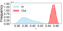
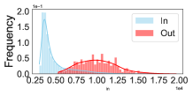
Fig. 2: Histogram scores.

4 Experimental Settings

In this section, we first discuss the limitation of the previous works on textual OOD detection, then present the chosen benchmark, the pretrained encoders, and baseline methods.

4.1 Previous works and their limitations

Previous works in OOD detection [62, 84, 52, 67, 75] mostly rely on a single model to determine which methods are the best. This undermines the soundness of the conclusions that may only hold for the particular instance of the chosen model (e.g. for a specific checkpoint trained with a specific seed). To the best of our knowledge, no work studies the impact of the several sources of randomness that are involved, such as checkpoint and seed selections [86]). Nevertheless, these hyperparameters do impact the OOD detectors’ performances. This is illustrated in Fig. 8 of the supplementary material, which gathers several Mahalanobis scores for various checkpoints of the same model.

In the light of Fig. 8, we choose to study both the impact of the checkpoint and the seed choice in our experiment. Specifically, for each model, we consider 5 different checkpoints. We save and probe models after 1k, 3k, 5k, 10k, 15k, and 20k finetuning steps. We additionally reproduce this experiment for 3 different seeds. As the reuse of checkpoints reduces the cost of research and allows for easy head-to-head comparison, our library also contains the probed models to draw general robust conclusions about the performance of the considered class of models [30, 38, 102].

4.2 Dataset selection

Dataset selection is instrumental for OOD detection evaluation as it is unreasonable to expect a detection method to achieve good results on any type of OOD data [1]. Since there is a lack of consensus on which benchmark to use for OOD detection in NLP, we choose to rely on the benchmark introduced by [103] which is an extension of the one proposed by [49].

Benchmark description. The considered benchmark is composed of three different types of in distribution datasets (referred to as IN-DS) which are used to train the classifiers: sentiment analysis (i.e., SST2 [88] and IMDB [70]), topic classification (i.e., 20Newsgroup [54]) and question answering (i.e., TREC-10 [61]). For splitting we use either the standard split or the one provided by [103]. For the OOD datasets (referred to as OUT-DS), we first consider the aforementioned datasets (i.e., any pair of datasets can be considered as OOD). Then, we also rely on four other datasets: a concatenation of premises and respective hypotheses from two NLI datasets (i.e., RTE [12, 51] and MNLI [99]), Multi30K [40] and the source of the English-German WMT16 [8]. We gather in Tab. 5 the statistics of the various data-sets and refer the reader to reference [103] for further details.

4.3 Baseline methods and pretrained models

Baseline methods. We consider the three following baselines:

1. Maximum Soft-max Probability (MSP). This method has been proposed by [47]. Given an input $\mathbf{x}$, it relies on the final score $s_{\mathrm{MSP}}$ defined by $s_{\mathrm{MSP}}(\mathbf{x})=1-\max_{y\in\mathcal{Y}}p_{Y|X}(y|\mathbf{x})$, where $p_{Y|X}(\cdot|x))$ is the soft-probability predicted by the classifier after $\mathbf{x}$ has been observed.

2. Energy-based score (E) [67] is defined as the score $s_{E}(\mathbf{x})=T\times\log\left[\sum_{y\in\mathcal{Y}}\exp\left(\frac{g_{y}(\mathbf{x})}{T}\right)\right]$, where $g_{y}(\mathbf{x})$ represents the logit corresponding to the class label $y$.

3. Mahalanobis ($D_{\mathrm{M}}$). Following [75, 60, 103], the last layer of the encoder is considered leading to the score: $s_{\mathrm{M}}(\mathbf{x})=-D_{\mathrm{M}}(F_{\mathrm{PM}}(\mathbf{x}),F_{\mathrm{PM}}(\mathcal{S}_{n,\hat{y}}^{\mathrm{train}}))$ where $\hat{y}$ represents the label predicted by the classifier based on the observation of $\mathbf{x}$.

Aggregation procedures. Both $D_{\mathrm{M}}$ and $D_{\mathrm{IRW}}$ rely on feature representations of the data which are extracted from the neural networks. Our goal is to demonstrate that our aggregation procedure $F_{PM}$ defined in Eq. 3 is a relevant choice to be plugged in Eq. 5. To do so, we also perform experiments on other natural aggregation strategies we introduce in the following.

1. Logits layer selection. We use the raw non-normalized predictions of the classifier. In this case $F_{Logits}\equiv F\left(\phi_{1}(\mathbf{x}),\dots,\phi_{L}(\mathbf{x})\right)=\phi_{L+1}(\mathbf{x})$.

2. Last layer selection. Following previous work in textual OOD detection [100], we also consider the last layer of the network. Formally $F_{L}\equiv F\left(\phi_{1}(\mathbf{x}),\dots,\phi_{L}(\mathbf{x})\right)=\phi_{L}(\mathbf{x})$.

3. Layer concatenation. We follow the BERT pooler and explore the concatenation of all layers. Formally, $F_{cat}\equiv F\left(\phi_{1}(\mathbf{x}),\dots,\phi_{L}(\mathbf{x})\right)=[\phi_{1}(\mathbf{x}),\cdots,\phi_{L}(\mathbf{x})]$ represents the concatenated vector. The main limitation of layer concatenation is that the dimension of the considered features linearly increases with the number of layers which can be problematic for very deep networks [98].

Pretrained encoders. To provide an exhaustive comparison, we choose to work with different types of pretrained encoders. We test the various methods on DISTILBERT (DIS.) [83], BERT [35] and ROBERTA (ROB.) [68]. We trained all models with a dropout rate [89] of $0.2$, a batch size of $32$, we use ADAMW [55]. Additionally, the weight decay is set to $0.01$, the warmup ratio is set to $0.06$ and the learning rate to $10^{-5}$.

IN-DS	BERT Acc	DIS. Acc	ROB. Acc
20ng	92.9	92.0	92.7
imdb	91.7	90.6	93.6
sst2	92.7	91.7	95.2
trec	96.8	97.0	97.0

Tab. 1: Average test accuracy achieved by different classifier when training is initialized with different seeds.

5 Static Experimental Results

In this section, we demonstrate the effectiveness of our proposed detector using various pretrained models. Due to space limitations, additional tables are reported in the Supplementary Material.

5.1 Methods comparison

Tab. 2: Average OOD detection performance (in %). The averages are taken over 1440 configurations and include four different IN-DS (20ng, imdb, sst2, trec), eight OOD-DS, three different seeds, five different checkpoints and three different pretrained encoders. Due to space constraints, different aggregations and related discussions are relegated to Appendix B.

Score	Aggregation	AUROC	AUPR-IN	AUPR-OUT	FPR	Err
$E$	$F_{L+1}$	89.9 $\pm{9.7}$	84.9 $\pm{19.0}$	79.9 $\pm{27.3}$	44.9 $\pm{33.4}$	23.9 $\pm{22.0}$
MSP	Soft.	89.7 $\pm{9.1}$	84.3 $\pm{18.9}$	80.4 $\pm{25.6}$	45.5 $\pm{29.5}$	25.4 $\pm{21.4}$
$D_{\mathrm{M}}$	$F_{L}$	93.8 $\pm{9.8}$	89.2 $\pm{20.1}$	91.5 $\pm{16.4}$	19.8 $\pm{23.7}$	12.7 $\pm{17.0}$
	$F_{L+1}$	71.7 $\pm{13.7}$	54.7 $\pm{32.0}$	73.3 $\pm{28.4}$	62.6 $\pm{23.1}$	37.0 $\pm{22.9}$
	$F_{[L,L+1]}$	81.7 $\pm{20.7}$	60.7 $\pm{20.0}$	83.8 $\pm{20.3}$	73.4 $\pm{23.5}$	33.0 $\pm{21.3}$
	$F_{L\oplus L+1}$	83.6 $\pm{10.6}$	61.9 $\pm{39.3}$	79.4 $\pm{26.9}$	81.5 $\pm{10.1}$	30.4 $\pm{18.8}$
	$F_{cat}$	90.4 $\pm{11.5}$	84.0 $\pm{22.1}$	88.0 $\pm{19.7}$	28.9 $\pm{26.2}$	17.6 $\pm{18.8}$
	$F_{\mathrm{PM}}$	81.2 $\pm{15.3}$	67.7 $\pm{28.7}$	82.1 $\pm{22.2}$	40.2 $\pm{28.0}$	23.1 $\pm{20.3}$
$D_{\mathrm{IRW}}$	$F_{L}$	92.6 $\pm{8.0}$	88.5 $\pm{17.7}$	86.3 $\pm{19.7}$	37.8 $\pm{27.3}$	23.6 $\pm{20.4}$
	$F_{L+1}$	82.4 $\pm{14.0}$	77.2 $\pm{24.0}$	72.1 $\pm{29.8}$	68.5 $\pm{29.5}$	38.0 $\pm{25.3}$
	$F_{[L,L+1]}$	95.5 $\pm{10.0}$	91.2 $\pm{15.0}$	94.1 $\pm{29.0}$	23.5 $\pm{31.5}$	13.7 $\pm{15.3}$
	$F_{L\oplus L+1}$	95.9 $\pm{10.0}$	91.0 $\pm{20.0}$	94.0 $\pm{11.0}$	15.5 $\pm{20.5}$	13.0 $\pm{16.0}$
	$F_{cat}$	96.1 $\pm{4.9}$	91.8 $\pm{14.0}$	94.1 $\pm{11.4}$	19.1 $\pm{21.6}$	14.1 $\pm{16.2}$
TRUSTED	$F_{\mathrm{PM}}$	97.0 $\pm{\textbf{4.0}}$	93.2 $\pm{\textbf{11.5}}$	95.1 $\pm{\textbf{10.0}}$	15.4 $\pm{\textbf{19.2}}$	11.7 $\pm{\textbf{13.7}}$

In Tab. 2, we report the aggregated score obtained by each method combined with a different aggregation function. We observe that TRUSTED obtains the best overall scores followed by $D_{\mathrm{IRW}}$ using $F_{cat}$. Similarly to previous works [75], we notice in general that score leveraging information available from the training set (i.e., $D_{\mathrm{M}}$ and $D_{\mathrm{IRW}}$) achieve stronger results than those relying on output of softmax scores solely (i.e., $E$ and MSP).

Interestingly, we observe that $D_{\mathrm{M}}$ achieves the best results when relying on the last layer solely (i.e., using $F_{L+1}$). Considering additional layers through concatenation or mean hurts the performances of $D_{\mathrm{M}}$. This is not the case when relying on $D_{IRW}$. Indeed layer aggregation improves the performance of the detector demonstrating the relevance of using $D_{IRW}$ over $D_{M}$ as an OOD score. Relying on Mahalanobis as OOD score suppose that the representation follows a multivariate Gaussian distribution which might be too strong assumption in the case of layer aggregation. On the contrary $D_{IRW}$ do not rely on any distributional assumption.

5.2 On the pretrained encoder choice

Tab. 3: Average (over 480 model configurations) performance per pretrained encoder type.

Model	Score	Aggregation	AUROC	AUPR-IN	AUPR-OUT	FPR	Err
BERT	MSP	Soft.	89.6 $\pm{9.3}$	84.1 $\pm{19.8}$	80.8 $\pm{25.5}$	46.4 $\pm{30.8}$	25.8 $\pm{22.4}$
	$E$	$F_{L+1}$	89.7 $\pm{9.9}$	85.2 $\pm{19.2}$	79.9 $\pm{28.2}$	45.5 $\pm{34.4}$	23.5 $\pm{22.2}$
	$D_{\mathrm{M}}$	$F_{L}$	95.9 $\pm{6.9}$	91.9 $\pm{17.3}$	93.1 $\pm{15.4}$	15.9 $\pm{21.5}$	10.7 $\pm{15.1}$
		$F_{L+1}$	70.7 $\pm{13.0}$	51.9 $\pm{31.5}$	74.3 $\pm{26.9}$	62.3 $\pm{22.2}$	37.4 $\pm{22.1}$
		$F_{cat}$	92.2 $\pm{8.8}$	81.9 $\pm{24.4}$	92.2 $\pm{12.4}$	29.3 $\pm{26.5}$	21.5 $\pm{21.6}$
		$F_{\mathrm{PM}}$	80.5 $\pm{16.0}$	65.9 $\pm{30.3}$	81.9 $\pm{21.8}$	42.1 $\pm{28.9}$	24.9 $\pm{21.6}$
	$D_{\mathrm{IRW}}$	$F_{L}$	92.6 $\pm{7.7}$	88.7 $\pm{18.2}$	87.0 $\pm{19.1}$	38.0 $\pm{27.8}$	23.8 $\pm{20.4}$
		$F_{L+1}$	81.1 $\pm{14.7}$	76.6 $\pm{24.8}$	71.7 $\pm{29.6}$	72.3 $\pm{29.4}$	40.8 $\pm{25.9}$
		$F_{cat}$	96.5 $\pm{5.2}$	92.1 $\pm{15.7}$	95.8 $\pm{9.2}$	15.9 $\pm{22.1}$	12.8 $\pm{17.9}$
	TRUSTED	$F_{\mathrm{PM}}$	97.4 $\pm{4.1}$	93.6 $\pm{12.8}$	96.4 $\pm{8.6}$	12.6 $\pm{19.6}$	10.4 $\pm{15.6}$
DIS.	MSP	Soft.	88.2 $\pm{9.7}$	82.7 $\pm{20.4}$	77.2 $\pm{27.9}$	51.6 $\pm{30.4}$	28.0 $\pm{22.7}$
	$E$	$F_{L+1}$	88.1 $\pm{10.9}$	83.3 $\pm{20.8}$	77.1 $\pm{29.4}$	50.3 $\pm{36.1}$	26.2 $\pm{24.1}$
	$D_{\mathrm{M}}$	$F_{L}$	94.1 $\pm{9.0}$	89.4 $\pm{20.2}$	90.6 $\pm{18.0}$	21.6 $\pm{24.3}$	13.8 $\pm{18.1}$
		$F_{L+1}$	72.3 $\pm{13.9}$	55.7 $\pm{33.1}$	72.3 $\pm{29.3}$	63.8 $\pm{23.1}$	37.8 $\pm{24.0}$
		$F_{cat}$	89.2 $\pm{11.6}$	83.9 $\pm{21.7}$	85.6 $\pm{21.5}$	30.8 $\pm{25.7}$	17.4 $\pm{18.2}$
		$F_{\mathrm{PM}}$	80.0 $\pm{15.6}$	68.6 $\pm{28.4}$	79.2 $\pm{24.7}$	43.8 $\pm{28.1}$	24.1 $\pm{20.8}$
	$D_{\mathrm{IRW}}$	$F_{L}$	91.2 $\pm{9.2}$	86.5 $\pm{19.9}$	84.6 $\pm{21.5}$	43.0 $\pm{28.1}$	26.8 $\pm{21.9}$
		$F_{L+1}$	78.4 $\pm{15.4}$	73.5 $\pm{25.5}$	67.8 $\pm{32.1}$	76.1 $\pm{26.3}$	41.7 $\pm{25.9}$
		$F_{cat}$	96.3 $\pm{3.9}$	91.5 $\pm{13.3}$	94.0 $\pm{11.7}$	18.9 $\pm{20.7}$	14.3 $\pm{14.9}$
	TRUSTED	$F_{\mathrm{PM}}$	97.3 $\pm{2.9}$	93.3 $\pm{10.4}$	95.1 $\pm{9.9}$	14.1 $\pm{17.1}$	11.1 $\pm{11.5}$
ROB.	MSP	Soft.	91.4 $\pm{7.9}$	85.9 $\pm{16.4}$	83.0 $\pm{23.0}$	39.1 $\pm{26.0}$	22.6 $\pm{18.7}$
	$E$	$F_{L+1}$	91.7 $\pm{8.0}$	86.2 $\pm{16.8}$	82.6 $\pm{24.1}$	39.2 $\pm{28.5}$	22.0 $\pm{19.5}$
	$D_{\mathrm{M}}$	$F_{L}$	91.7 $\pm{11.9}$	86.6 $\pm{22.0}$	90.9 $\pm{15.5}$	21.6 $\pm{24.7}$	13.5 $\pm{17.5}$
		$F_{L+1}$	72.1 $\pm{14.0}$	56.1 $\pm{31.4}$	73.4 $\pm{28.8}$	61.7 $\pm{23.8}$	35.9 $\pm{22.4}$
		$F_{cat}$	89.8 $\pm{13.1}$	85.9 $\pm{20.0}$	86.5 $\pm{22.5}$	26.8 $\pm{26.4}$	14.4 $\pm{15.8}$
		$F_{\mathrm{PM}}$	82.8 $\pm{14.4}$	68.4 $\pm{27.4}$	85.0 $\pm{19.7}$	35.1 $\pm{26.5}$	20.5 $\pm{18.2}$
	$D_{\mathrm{IRW}}$	$F_{L}$	93.8 $\pm{6.6}$	90.2 $\pm{14.7}$	87.4 $\pm{18.2}$	32.9 $\pm{25.3}$	20.5 $\pm{18.4}$
		$F_{L+1}$	87.2 $\pm{10.0}$	81.0 $\pm{21.0}$	76.4 $\pm{27.2}$	58.1 $\pm{29.4}$	32.2 $\pm{23.2}$
		$F_{cat}$	95.7 $\pm{5.5}$	91.9 $\pm{13.1}$	92.6 $\pm{12.6}$	22.1 $\pm{21.8}$	15.2 $\pm{15.6}$
	TRUSTED	$F_{\mathrm{PM}}$	96.3 $\pm{4.7}$	92.7 $\pm{11.3}$	93.9 $\pm{11.2}$	19.1 $\pm{20.2}$	13.4 $\pm{13.8}$

When training and deploying a classifier, a key question is choosing a pretrained encoder. It can be beneficial in critical applications to trade off the main task accuracy to ensure better OOD detection. In Tab. 3, we report the individual performance of OOD methods on three types of classifiers. Although TRUSTED achieves state-of-the-art on all configurations, it is worth noticing a difference in performance concerning the type of pretrained model. It is also important to remark that for ROB both MSP and $E$ achieve on-par performances with $D_{\mathrm{M}}$ while not requiring any extra training information. Overall, for a given method (i.e. $D_{\mathrm{M}}$ or $D_{\mathrm{IRW}}$), the ranking of detectors performances according to the type of feature extractor remain still. This validates the use of the mean-aggregation procedure of TRUSTED. Overall, based on the difference of OOD detection performance of Tab. 3, we recommend to use TRUSTED on BERT or DIS. if accurate OOD detection is required.

5.3 Impact of the training dataset

OOD detection performance depends on the nature of what is considered in-distribution (the training distribution in our case). Thus, it is interesting to study the performance per-IN-DS as reported in Tab. 4. Even though TRUSTED achieves strong results in terms of AUROC, we observe a high FPR on SST2. From Fig. 3, we observe that IMDB and SST2 are harder to detect, especially for $D_{\mathrm{M}}$. Finally, since high AUROC does not necessarily imply a low FPR, it is crucial to take both into account when designing an OOD detector.

Fig. 3: AUROC&FPR trade-off.

		AUROC	AUPR-IN	AUPR-OUT	FPR	Err
IN-DS	Score
20ng	TRUSTED	98.4 $\pm{1.8}$	96.8 $\pm{4.8}$	98.0 $\pm{4.2}$	8.0 $\pm{10.5}$	6.4 $\pm{6.8}$
	$D_{\mathrm{M}}$	97.6 $\pm{4.6}$	95.1 $\pm{9.9}$	97.4 $\pm{6.4}$	10.1 $\pm{13.6}$	7.6 $\pm{7.5}$
imdb	TRUSTED	98.6 $\pm{2.1}$	99.8 $\pm{0.4}$	88.6 $\pm{15.5}$	8.0 $\pm{13.9}$	5.2 $\pm{2.0}$
	$D_{\mathrm{M}}$	93.3 $\pm{9.8}$	98.0 $\pm{5.4}$	77.3 $\pm{24.7}$	19.3 $\pm{20.6}$	6.4 $\pm{2.8}$
sst2	TRUSTED	93.8 $\pm{5.8}$	86.0 $\pm{17.2}$	93.9 $\pm{9.4}$	30.7 $\pm{22.9}$	22.1 $\pm{17.9}$
	$D_{\mathrm{M}}$	86.3 $\pm{12.3}$	71.7 $\pm{29.8}$	90.5 $\pm{12.9}$	43.0 $\pm{25.2}$	30.4 $\pm{22.9}$
trec	TRUSTED	97.6 $\pm{2.3}$	91.8 $\pm{8.1}$	99.3 $\pm{1.1}$	12.2 $\pm{15.3}$	11.0 $\pm{12.7}$
	$D_{\mathrm{M}}$	99.0 $\pm{1.2}$	94.9 $\pm{6.8}$	99.8 $\pm{0.4}$	4.4 $\pm{7.4}$	4.3 $\pm{6.2}$

Tab. 4: Average OOD detection performance per IN-DS.

6 Dynamic Experimental Results

Most OOD detection methods are tested on specific checkpoints, where the selection criterion is often unclear. The consequences of this selection on OOD detection are rarely studied. This section aims to respond to this by measuring the OOD detection performance of methods on various checkpoint finetuning of the pretrained encoder. We will use 5 different checkpoints taken after 1k, 3k, 5k, 10k, 15k, and 20k iterations. Training curves of the models are given in Fig. 6. Notice that after 3k iterations models have converged and no over-fitting is observed even after 20k iterations (i.e., we do not observe an increase in validation loss).

Overall analysis. We report the results of the dynamic analysis on the various pretrained models in Fig. 4. For all the methods and models (except $D_{\mathrm{M}}$ on ROB), we observe that training longer the classifier hurts detection. Interestingly, this drop in performance has a higher impact on FPR compared to AUROC. Thus, it is better to use an early stopping criterion to ensure proper OOD detection performance. In addition, we observed that TRUSTED (corresponding to $D_{\mathrm{IRW}}$) achieves better detection results and that $D_{\mathrm{M}}$ outperforms TRUSTED for checkpoints larger than 10k on ROB.

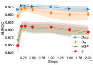
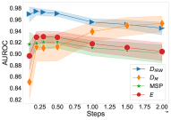
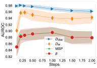
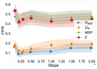
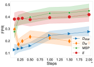
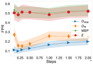
Fig. 4: Detection performance of different pretrained encoder during finetuning. First column correspond to BERT, second to ROB and last to DIS.

Analysis Per In-Dataset. Fig. 5 reports the results of the dynamical analysis per IN-DS. We observe that $D_{\mathrm{IRW}}$ is consistently better than $D_{\mathrm{M}}$ with sensible improvement on IMDB and SST2, which are the hardest benchmarks. We observe a similar trend to the previous experiment: training longer the classifiers hurt their OOD detection performances. Similar observations hold for FPR, AUPR-IN, and AUPR-OUT that are postponed to the Supplementary Material (see Fig. 9).

Fig. 5: AUROC per IN-DS during fine-tuning.

7 Conclusions and Future Directions

In this work, we introduced TRUSTED a novel OOD detector that relies on information available in all the hidden layers of a network. TRUSTED leverages a novel similarity score built on top of the Integrate Rank-Weighted depth. We conduct extensive numerical experiments proving that it consistently outperforms previous approaches, including detection based on the Mahalanobis distance. Our comprehensive evaluation framework demonstrates that, in general, OOD performances vary depending on several hyperparameters of the models, the datasets, and the detector’s feature extraction step. Thus, we would like to promote the use of such exhaustive evaluation frameworks for future search to assess AI systems’ safety tools properly. Another interesting question is the detection inference-time / accuracy trade-off, which is instrumental for the practitioner.

Checklist

1. For all authors…

   1. Do the main claims made in the abstract and introduction accurately reflect the paper’s contributions and scope? [Yes] We have backed all of our claims in the abstract and introduction throughout the work. See the summary of our contributions at Section 1.1.

   2. Did you describe the limitations of your work? [Yes] Please see Section CITE.

   3. Did you discuss any potential negative societal impacts of your work? [N/A] Our works aim at developing safer AI systems, so we believe our does not have any negative societal impact.

   4. Have you read the ethics review guidelines and ensured that your paper conforms to them? [Yes]

2. If you are including theoretical results…

   1. Did you state the full set of assumptions of all theoretical results? [N/A]

   2. Did you include complete proofs of all theoretical results? [N/A]

3. If you ran experiments…

   1. Did you include the code, data, and instructions needed to reproduce the main experimental results (either in the supplemental material or as a URL)? [Yes] We include extensive instructions to reproduce the main experimental results in both the supplementary material and main paper.

   2. Did you specify all the training details (e.g., data splits, hyperparameters, how they were chosen)? [Yes] We provide an extensive analysis on the hyperparamters for training the models and reproducing the results in the supplementary material.

   3. Did you report error bars (e.g., with respect to the random seed after running experiments multiple times)? [Yes] We report error bars in all of our main results (please see Sections 5 and  6).

   4. Did you include the total amount of compute and the type of resources used (e.g., type of GPUs, internal cluster, or cloud provider)? [Yes] We provide a rough estimate of the amount of compute used in the supplementary material.

4. If you are using existing assets (e.g., code, data, models) or curating/releasing new assets…

   1. If your work uses existing assets, did you cite the creators? [Yes] We cite all the datasets we use in the experimental setup of this work in the main paper.

   2. Did you mention the license of the assets? [N/A]

   3. Did you include any new assets either in the supplemental material or as a URL? [Yes] We open-source our code in the supplementary material.

   4. Did you discuss whether and how consent was obtained from people whose data you’re using/curating? [N/A]

   5. Did you discuss whether the data you are using/curating contains personally identifiable information or offensive content? [N/A]

5. If you used crowdsourcing or conducted research with human subjects…

   1. Did you include the full text of instructions given to participants and screenshots, if applicable? [N/A]

   2. Did you describe any potential participant risks, with links to Institutional Review Board (IRB) approvals, if applicable? [N/A]

   3. Did you include the estimated hourly wage paid to participants and the total amount spent on participant compensation? [N/A]

[sections] [sections]l1

Appendix A Experimental Details

In this section we gather additional experimental details. For completeness we provide the used algorithms for both TRUSTED and $D_{\mathrm{IRW}}$ (see Sec. A.1), we also gather additional benchmarks details (see Sec. A.2), hyperparameter used during training (see Sec. A.3) as well as the training curves (see Sec. A.4).

A.1 Algorithms

In this part, we present algorithms to compute $D_{\mathrm{IRW}}$ (see Algorithm 1) and TRUSTED (see Algorithm 2).

Algorithm 1 Approximation of the IRW depth

Initialization: test sample $x$, $n_{\mathrm{proj}}$, $\mathbf{X}=[x_{1},\ldots,x_{n}]^{\top}$.

1:  Construct $\mathbf{U}\in\mathbb{R}^{d\times n_{\mathrm{proj}}}$ by sampling uniformly $n_{\mathrm{proj}}$ vectors $U_{1},\ldots,U_{n_{\mathrm{proj}}}$ in $\mathbb{S}^{d-1}$

2:  Compute $\mathbf{M}=\mathbf{XU}$ and $x^{\top}\mathbf{U}$

3:  Compute the rank value $\sigma(j)$, the rank of $x^{\top}\mathbf{U}$ in $\mathbf{M}_{:,j}$ for every $j\leq n_{\mathrm{proj}}$

4:  Set $D=\frac{1}{n_{\mathrm{proj}}}\sum_{j=1}^{n_{\mathrm{proj}}}\;\;\sigma(j)$ Output: $\widetilde{D}_{\mathrm{IRW}}(x,\mathbf{X})=D$

Algorithm 2 Computation of TRUSTED

Initialization: $\mathbf{x}$, $n_{\mathrm{proj}}$, $\mathcal{S}_{n}$, $\hat{y}$.

1:  Compute $F_{\mathrm{PM}}(\mathbf{x})$

2:  for  $y=1,\ldots,C$ do

3:     Compute $F_{\mathrm{PM}}(\mathcal{S}_{n,y}^{\mathrm{train}})$

4:  end for

5:  Compute $D_{\mathrm{IRW}}(F_{\mathrm{PM}}(\mathbf{x}),F_{\mathrm{PM}}(\mathcal{S}_{n,\hat{y}}^{\mathrm{train}}))$ using Algorithm 1 with $F_{\mathrm{PM}}(\mathbf{x})$, $n_{\mathrm{proj}}$ and $F_{\mathrm{PM}}(\mathcal{S}_{n,\hat{y}}^{\mathrm{train}})$ Output: $s_{\texttt{TRUSTED}}(\mathbf{x})=D_{\mathrm{IRW}}(F_{\mathrm{PM}}(\mathbf{x}),F_{\mathrm{PM}}(\mathcal{S}_{n,\hat{y}}^{\mathrm{train}}))$

A.2 Benchmark Details

We report in Tab. 5 statistics related to the datasets of our benchmark. The only difference between our work and the one from [103] is that we considered the pair IMDB and SST2 a valid OOD pair of IN-DS/OOD-DS as this can be seen as a background shift (see [78]).

Remark 1

We initially started to work with the appealing benchmark introduced by [60] which introduces an alternative standard that addresses the limitation of the benchmark proposed by [100] (e.g. there is no category overlap between training and OOD test examples in the non-semantic shift dataset). Additionally, [60] put effort into designing a dataset that can categorize shifts as belonging to semantic or background shift [2, 78]. However, we failed to reproduce the baseline results from [60] even after contacting the authors.

Dataset	#train	#dev	#test	#class
SST2	67349	872	1821	2
IMDB	22500	2500	25000	2
TREC10	4907	545	500	6
20NG	15056	1876	1896	20
MNLI	-	-	19643	-
RTE	-	-	3000	-
Multi30K	-	-	2532	-
WMT16	-	-	2999	-

Tab. 5: Statistics of the considered benchmark.

A.3 Training Parameters

In this section, the detail the main hyper-parameters that were used for finetuning the pretrained encoders. It is worth noting that we use the same set of hyperparameters for all the different encoders [26, 24]. The dropout rate [89] is set to $0.2$ [], we train with a batch size of $32$, we use ADAMW [55, 69, 4]. Additionally, we set the weight decay to $0.01$, the warmup ratio to $0.06$, and the learning rate to $10^{-5}$. All the models were trained during 20k iterations with different seeds.

A.4 Training Curves

In order to understand the change of performance while finetuning the model, it is crucial to understand when and if the different models have converged. Thus we report in Fig. 6 dev losses and dev and test accuracy. From Fig. 6, we can observe that a pretrained encoder finetuned on 20ng takes more time to converge compared to the same pretrained encoder finetuned on either SST2, IMDB, or trec. Additionally, after 2k updates, both dev and test accuracy are stable on SST2, IMDB, and trec, while for 20ng, it requires 6k steps. Last, it is worth noting (see Tab. 1) that ROB. achieves the best accuracy overall. BERT is the second best and achieves stronger test accuracy than DIS. on the different datasets.

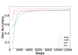
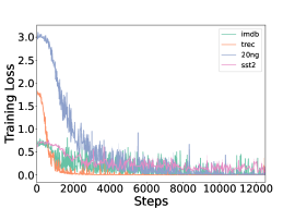
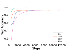
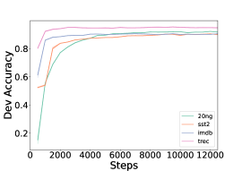
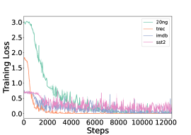
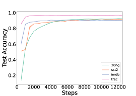
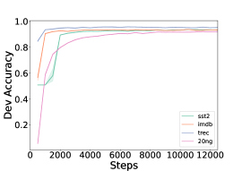
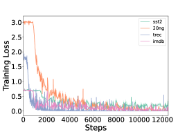
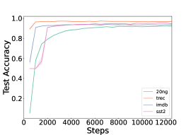
Fig. 6: Dev and Test curves obtained during finetuning of the pretrained transformers on different datasets for the three considered seeds.

Appendix B Additional Static Experimental Results

In this section, we report additional static experiment results. Formally, we aim to gain understanding:

• on the role of the IN-DS (see Sec. B.1) and on the impact of the choice of the pretrained encoder [27].

• on the different trade-off that exists between the different metrics (see Sec. B.2)

• on the impact of performance of the detection methods depending on the OOD distribution (see Sec. B.3).

B.1 Analysis Per In-Dataset

We present in Tab. 6 the average performance per IN-DS. On 3 out of 4 datasets TRUSTED achieves the best results and outperforms other methods. Interestingly, the table shows the key importance of the training corpus. As an example, we observe that detection methods applied to classifiers trained on sst2 are less efficient (by several AUROC points) compared to other IN-DS.
A finer analysis of this phenomenon can be conducted using Tab. 7. From Tab. 7, we observe that this phenomenon is consistent accross all the pretrained classifiers (i.e., BERT, ROB. and DIS.). We observe that different TRUSTED does not work uniformly better on all pretrained models. For example, the best results on 20ng are obtained for BERT while on sst2 it is obtained for DIS..
Takeaways: Both IN-DS and pretrained model choices are essential to ensure good detection performance.

Tab. 6: Average OOD detection performance (in %) per IN-DS.

		AUROC	AUPR-IN	AUPR-OUT	FPR	Err
Score	Method
20ng	TRUSTED	98.4 $\pm{1.8}$	96.8 $\pm{4.8}$	98.0 $\pm{4.2}$	8.0 $\pm{10.5}$	6.4 $\pm{6.8}$
	$D_{\mathrm{M}}$	97.6 $\pm{4.6}$	95.1 $\pm{9.9}$	97.4 $\pm{6.4}$	10.1 $\pm{13.6}$	7.6 $\pm{7.5}$
	$E$	94.9 $\pm{3.7}$	88.4 $\pm{10.2}$	95.4 $\pm{6.5}$	21.3 $\pm{17.1}$	14.8 $\pm{11.5}$
	MSP	92.6 $\pm{4.8}$	85.0 $\pm{12.0}$	93.5 $\pm{8.3}$	31.1 $\pm{16.3}$	20.8 $\pm{11.0}$
imdb	TRUSTED	98.6 $\pm{2.1}$	99.8 $\pm{0.4}$	88.6 $\pm{15.5}$	8.0 $\pm{13.9}$	5.2 $\pm{2.0}$
	$D_{\mathrm{M}}$	93.3 $\pm{9.8}$	98.0 $\pm{5.4}$	77.3 $\pm{24.7}$	19.3 $\pm{20.6}$	6.4 $\pm{2.8}$
	$E$	87.7 $\pm{9.0}$	97.9 $\pm{2.7}$	40.0 $\pm{24.2}$	64.4 $\pm{27.3}$	12.8 $\pm{8.9}$
	MSP	89.7 $\pm{7.5}$	98.2 $\pm{2.1}$	43.3 $\pm{22.5}$	56.2 $\pm{22.5}$	12.0 $\pm{7.8}$
sst2	TRUSTED	93.8 $\pm{5.8}$	86.0 $\pm{17.2}$	93.9 $\pm{9.4}$	30.7 $\pm{22.9}$	22.1 $\pm{17.9}$
	$D_{\mathrm{M}}$	86.3 $\pm{12.3}$	71.7 $\pm{29.8}$	90.5 $\pm{12.9}$	43.0 $\pm{25.2}$	30.4 $\pm{22.9}$
	$E$	80.8 $\pm{10.0}$	70.6 $\pm{25.9}$	81.9 $\pm{17.0}$	76.2 $\pm{18.9}$	50.1 $\pm{21.7}$
	MSP	81.2 $\pm{10.0}$	71.3 $\pm{25.7}$	82.6 $\pm{16.1}$	75.8 $\pm{17.3}$	50.1 $\pm{21.4}$
trec	TRUSTED	97.6 $\pm{2.3}$	91.8 $\pm{8.1}$	99.3 $\pm{1.1}$	12.2 $\pm{15.3}$	11.0 $\pm{12.7}$
	$D_{\mathrm{M}}$	99.0 $\pm{1.2}$	94.9 $\pm{6.8}$	99.8 $\pm{0.4}$	4.4 $\pm{7.4}$	4.3 $\pm{6.2}$
	$E$	96.9 $\pm{3.3}$	85.6 $\pm{13.9}$	99.3 $\pm{1.0}$	15.5 $\pm{15.3}$	13.9 $\pm{12.7}$
	MSP	96.2 $\pm{3.4}$	85.1 $\pm{13.7}$	99.1 $\pm{1.2}$	16.9 $\pm{15.8}$	15.2 $\pm{13.2}$

Tab. 7: Average OOD detection performance (in %) per IN-DS and per pretrained encoders.

			AUROC	AUPR-IN	AUPR-OUT	FPR	Err
IN DS	MODEL	TECH
20ng	BERT	TRUSTED	99.9 $\pm{0.3}$	99.4 $\pm{1.4}$	100.0 $\pm{0.0}$	0.4 $\pm{0.9}$	1.0 $\pm{1.0}$
		$D_{\mathrm{M}}$	98.8 $\pm{1.7}$	97.6 $\pm{2.6}$	98.4 $\pm{4.6}$	6.1 $\pm{8.7}$	5.1 $\pm{3.8}$
		$E$	95.4 $\pm{3.8}$	89.0 $\pm{10.1}$	95.9 $\pm{6.1}$	21.0 $\pm{20.0}$	15.0 $\pm{13.6}$
		MSP	93.7 $\pm{4.1}$	86.4 $\pm{11.7}$	94.8 $\pm{6.0}$	28.1 $\pm{15.6}$	19.5 $\pm{11.1}$
	Dist	TRUSTED	99.0 $\pm{0.7}$	97.8 $\pm{2.6}$	99.0 $\pm{1.4}$	3.5 $\pm{4.0}$	4.3 $\pm{2.7}$
		$D_{\mathrm{M}}$	97.7 $\pm{4.2}$	96.0 $\pm{5.6}$	97.0 $\pm{9.0}$	10.9 $\pm{16.7}$	7.8 $\pm{8.1}$
		$E$	96.4 $\pm{3.0}$	91.2 $\pm{7.8}$	96.9 $\pm{4.8}$	15.7 $\pm{14.9}$	11.6 $\pm{10.4}$
		MSP	93.9 $\pm{4.1}$	86.8 $\pm{11.1}$	95.2 $\pm{5.6}$	25.6 $\pm{15.0}$	17.8 $\pm{10.5}$
	Rob	TRUSTED	96.8 $\pm{1.7}$	94.0 $\pm{6.0}$	95.6 $\pm{5.8}$	17.2 $\pm{10.7}$	12.1 $\pm{7.0}$
		$D_{\mathrm{M}}$	96.5 $\pm{5.9}$	92.3 $\pm{14.2}$	96.9 $\pm{5.4}$	12.9 $\pm{13.8}$	9.4 $\pm{8.7}$
		$E$	93.5 $\pm{3.6}$	85.9 $\pm{11.2}$	94.0 $\pm{7.5}$	25.3 $\pm{14.6}$	16.8 $\pm{10.0}$
		MSP	90.7 $\pm{5.1}$	82.7 $\pm{12.4}$	91.4 $\pm{10.6}$	37.3 $\pm{15.8}$	23.9 $\pm{10.7}$
imdb	BERT	TRUSTED	98.9 $\pm{1.8}$	99.9 $\pm{0.2}$	91.1 $\pm{14.8}$	5.6 $\pm{11.1}$	4.7 $\pm{1.0}$
		$D_{\mathrm{M}}$	96.5 $\pm{5.4}$	99.5 $\pm{0.8}$	80.9 $\pm{24.3}$	13.9 $\pm{18.7}$	5.5 $\pm{1.6}$
		$E$	85.6 $\pm{9.8}$	97.6 $\pm{3.2}$	34.4 $\pm{22.3}$	73.8 $\pm{21.1}$	13.9 $\pm{9.5}$
		MSP	89.2 $\pm{7.0}$	98.1 $\pm{2.3}$	41.3 $\pm{21.8}$	60.5 $\pm{20.3}$	12.6 $\pm{8.3}$
	Dist	TRUSTED	98.8 $\pm{1.8}$	99.8 $\pm{0.3}$	89.2 $\pm{13.2}$	6.2 $\pm{10.5}$	4.9 $\pm{1.2}$
		$D_{\mathrm{M}}$	95.0 $\pm{6.6}$	99.2 $\pm{1.0}$	75.9 $\pm{26.8}$	20.2 $\pm{21.3}$	6.3 $\pm{2.4}$
		$E$	86.2 $\pm{9.1}$	97.7 $\pm{2.9}$	38.6 $\pm{25.6}$	69.1 $\pm{27.5}$	13.3 $\pm{9.3}$
		MSP	88.0 $\pm{7.8}$	98.0 $\pm{2.3}$	39.0 $\pm{21.6}$	64.1 $\pm{17.6}$	12.9 $\pm{8.2}$
	Rob	TRUSTED	98.2 $\pm{2.7}$	99.7 $\pm{0.6}$	86.0 $\pm{17.8}$	12.1 $\pm{17.9}$	5.9 $\pm{3.0}$
		$D_{\mathrm{M}}$	88.6 $\pm{13.3}$	95.3 $\pm{8.5}$	75.9 $\pm{22.5}$	22.7 $\pm{20.7}$	7.2 $\pm{3.7}$
		$E$	91.2 $\pm{7.2}$	98.5 $\pm{1.8}$	46.3 $\pm{22.9}$	51.4 $\pm{26.8}$	11.4 $\pm{7.8}$
		MSP	92.0 $\pm{7.1}$	98.6 $\pm{1.7}$	49.6 $\pm{22.8}$	43.9 $\pm{23.7}$	10.6 $\pm{6.8}$
sst2	BERT	TRUSTED	93.2 $\pm{5.3}$	83.4 $\pm{19.1}$	94.4 $\pm{7.1}$	32.0 $\pm{23.0}$	25.1 $\pm{20.4}$
		$D_{\mathrm{M}}$	90.1 $\pm{9.4}$	78.1 $\pm{26.7}$	91.7 $\pm{14.2}$	36.8 $\pm{23.9}$	25.8 $\pm{20.5}$
		$E$	81.2 $\pm{9.2}$	70.4 $\pm{26.2}$	82.8 $\pm{17.0}$	75.5 $\pm{15.6}$	49.5 $\pm{20.4}$
		MSP	80.2 $\pm{9.5}$	69.3 $\pm{27.0}$	81.7 $\pm{16.0}$	80.0 $\pm{8.9}$	52.7 $\pm{20.2}$
	Dist	TRUSTED	95.1 $\pm{3.2}$	87.5 $\pm{14.4}$	93.8 $\pm{11.3}$	26.2 $\pm{18.7}$	17.8 $\pm{11.6}$
		$D_{\mathrm{M}}$	86.5 $\pm{12.2}$	71.9 $\pm{30.8}$	91.0 $\pm{11.9}$	43.8 $\pm{25.5}$	31.6 $\pm{25.0}$
		$E$	76.3 $\pm{8.8}$	65.9 $\pm{27.1}$	77.4 $\pm{18.9}$	86.1 $\pm{13.6}$	55.9 $\pm{21.1}$
		MSP	77.7 $\pm{8.5}$	67.7 $\pm{26.5}$	79.0 $\pm{17.7}$	85.0 $\pm{5.9}$	55.4 $\pm{19.6}$
	Rob	TRUSTED	93.2 $\pm{7.7}$	87.2 $\pm{17.5}$	93.6 $\pm{9.6}$	34.0 $\pm{25.9}$	23.5 $\pm{19.7}$
		$D_{\mathrm{M}}$	82.3 $\pm{13.7}$	65.1 $\pm{30.4}$	88.9 $\pm{12.3}$	48.2 $\pm{25.1}$	33.7 $\pm{22.5}$
		$E$	84.9 $\pm{10.2}$	75.6 $\pm{23.4}$	85.5 $\pm{13.7}$	67.0 $\pm{21.6}$	44.8 $\pm{22.1}$
		MSP	85.8 $\pm{10.3}$	76.8 $\pm{22.5}$	87.0 $\pm{13.3}$	62.5 $\pm{22.6}$	42.2 $\pm{22.2}$
trec	BERT	TRUSTED	98.6 $\pm{1.4}$	95.0 $\pm{5.5}$	99.6 $\pm{0.6}$	7.2 $\pm{11.9}$	6.7 $\pm{9.9}$
		$D_{\mathrm{M}}$	99.3 $\pm{0.7}$	96.5 $\pm{4.6}$	99.8 $\pm{0.2}$	2.3 $\pm{3.7}$	2.5 $\pm{3.1}$
		$E$	97.6 $\pm{2.6}$	88.4 $\pm{11.7}$	99.5 $\pm{0.7}$	10.2 $\pm{10.3}$	9.3 $\pm{8.5}$
		MSP	96.9 $\pm{2.8}$	87.4 $\pm{11.3}$	99.3 $\pm{0.9}$	12.6 $\pm{11.6}$	11.4 $\pm{9.6}$
	Dist	TRUSTED	97.0 $\pm{2.8}$	89.9 $\pm{8.9}$	99.2 $\pm{1.2}$	16.6 $\pm{17.5}$	14.8 $\pm{14.5}$
		$D_{\mathrm{M}}$	98.6 $\pm{1.6}$	93.4 $\pm{7.5}$	99.7 $\pm{0.5}$	7.8 $\pm{10.6}$	7.3 $\pm{8.8}$
		$E$	95.9 $\pm{4.1}$	82.1 $\pm{15.6}$	99.1 $\pm{1.3}$	20.7 $\pm{19.1}$	18.3 $\pm{16.0}$
		MSP	94.9 $\pm{4.4}$	80.8 $\pm{16.1}$	98.7 $\pm{1.5}$	24.3 $\pm{19.9}$	21.5 $\pm{16.5}$
	Rob	TRUSTED	97.3 $\pm{2.1}$	90.9 $\pm{8.5}$	99.1 $\pm{1.2}$	12.2 $\pm{14.4}$	11.0 $\pm{11.5}$
		$D_{\mathrm{M}}$	99.1 $\pm{0.9}$	95.0 $\pm{7.4}$	99.8 $\pm{0.3}$	2.6 $\pm{4.1}$	2.8 $\pm{3.4}$
		$E$	97.1 $\pm{2.5}$	86.6 $\pm{13.2}$	99.3 $\pm{0.9}$	14.8 $\pm{12.7}$	13.3 $\pm{10.4}$
		MSP	97.0 $\pm{2.0}$	87.5 $\pm{11.8}$	99.3 $\pm{0.8}$	13.3 $\pm{11.1}$	12.0 $\pm{9.1}$

B.2 Trade-off between metrics

We report Fig. 7 the different trade-off that exist between the considered metrics. Interestingly, a high AUROC does not imply a low FPR. Similar conclusions can be drawn regarding AUPR-IN and AUPR-OUT.
Takeaways. Fig. 7 illustrates that all metrics matters and should be considered when comparing detection methods.

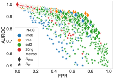
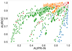
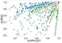
Fig. 7: Trade-off between different metrics for all considered configurations.

B.3 Analysis Per Out-Dataset

We report on Tab. 8 the detailled results of the detection methods for different OUT-DS. It is worth noting that TRUSTED achieves best results on 22 configurations.
Takeaways. Tab. 8 illustrates the impact of the type of OOD sample on the detection performances.

				AUROC	AUPR-IN	AUPR-OUT	FPR	Err
OUT DS	MODEL	TECH	Feature Type
20ng	BERT	TRUSTED		97.9 $\pm{2.2}$	99.2 $\pm{0.7}$	87.2 $\pm{19.2}$	11.6 $\pm{14.6}$	4.6 $\pm{4.3}$
		$D_{\mathrm{M}}$	Pooled	97.4 $\pm{2.6}$	98.2 $\pm{2.2}$	92.0 $\pm{10.3}$	13.6 $\pm{14.8}$	7.7 $\pm{7.7}$
		$E$	Energy	91.1 $\pm{7.5}$	95.3 $\pm{4.8}$	72.3 $\pm{30.9}$	48.8 $\pm{36.1}$	18.4 $\pm{17.1}$
		MSP	softmax	91.1 $\pm{6.8}$	95.0 $\pm{5.1}$	72.7 $\pm{28.9}$	49.1 $\pm{34.1}$	19.4 $\pm{17.4}$
	Dist	TRUSTED		98.7 $\pm{1.7}$	99.5 $\pm{0.7}$	90.7 $\pm{14.6}$	6.0 $\pm{9.9}$	3.3 $\pm{2.0}$
		$D_{\mathrm{M}}$	Pooled	97.0 $\pm{4.5}$	97.7 $\pm{5.0}$	92.3 $\pm{11.2}$	13.9 $\pm{16.6}$	7.6 $\pm{7.9}$
		$E$	Energy	87.7 $\pm{10.1}$	93.7 $\pm{7.6}$	65.7 $\pm{32.4}$	56.9 $\pm{41.0}$	20.7 $\pm{20.3}$
		MSP	softmax	89.1 $\pm{8.3}$	94.3 $\pm{6.2}$	67.9 $\pm{31.0}$	53.1 $\pm{36.6}$	19.9 $\pm{18.7}$
	Rob	TRUSTED		98.6 $\pm{1.5}$	99.1 $\pm{1.1}$	92.9 $\pm{11.5}$	7.7 $\pm{12.3}$	4.7 $\pm{5.4}$
		$D_{\mathrm{M}}$	Pooled	91.5 $\pm{11.0}$	92.5 $\pm{12.1}$	86.3 $\pm{16.0}$	23.9 $\pm{28.7}$	12.1 $\pm{14.9}$
		$E$	Energy	95.3 $\pm{4.3}$	97.0 $\pm{4.4}$	79.6 $\pm{24.3}$	30.2 $\pm{27.4}$	12.3 $\pm{12.7}$
		MSP	softmax	94.7 $\pm{6.8}$	96.2 $\pm{8.1}$	79.6 $\pm{23.8}$	28.0 $\pm{24.9}$	11.8 $\pm{12.3}$
imdb	BERT	TRUSTED		95.1 $\pm{5.6}$	80.1 $\pm{21.3}$	99.5 $\pm{0.7}$	21.3 $\pm{26.2}$	20.2 $\pm{24.4}$
		$D_{\mathrm{M}}$	Pooled	90.2 $\pm{13.4}$	69.5 $\pm{35.8}$	98.9 $\pm{1.7}$	27.9 $\pm{36.0}$	26.3 $\pm{33.6}$
		$E$	Energy	87.3 $\pm{14.9}$	62.5 $\pm{31.0}$	98.5 $\pm{2.0}$	37.2 $\pm{38.7}$	35.0 $\pm{36.1}$
		MSP	softmax	86.2 $\pm{14.6}$	59.5 $\pm{30.2}$	98.3 $\pm{2.0}$	41.7 $\pm{37.4}$	39.2 $\pm{34.8}$
	Dist	TRUSTED		96.1 $\pm{2.6}$	79.9 $\pm{13.9}$	99.7 $\pm{0.2}$	19.1 $\pm{15.0}$	18.4 $\pm{14.3}$
		$D_{\mathrm{M}}$	Pooled	86.0 $\pm{17.6}$	64.0 $\pm{38.8}$	98.2 $\pm{2.4}$	36.6 $\pm{42.6}$	34.5 $\pm{39.7}$
		$E$	Energy	84.9 $\pm{16.6}$	56.1 $\pm{31.5}$	98.0 $\pm{2.6}$	44.5 $\pm{39.7}$	42.0 $\pm{37.0}$
		MSP	softmax	84.7 $\pm{15.3}$	55.2 $\pm{29.6}$	98.1 $\pm{2.3}$	46.6 $\pm{35.9}$	44.0 $\pm{33.3}$
	Rob	TRUSTED		95.3 $\pm{7.4}$	80.6 $\pm{20.7}$	99.5 $\pm{0.9}$	18.3 $\pm{24.1}$	17.5 $\pm{22.5}$
		$D_{\mathrm{M}}$	Pooled	89.5 $\pm{16.3}$	68.6 $\pm{35.0}$	98.6 $\pm{2.5}$	25.0 $\pm{36.9}$	23.5 $\pm{34.4}$
		$E$	Energy	89.9 $\pm{12.6}$	64.8 $\pm{23.1}$	98.8 $\pm{1.7}$	35.2 $\pm{34.6}$	33.2 $\pm{32.2}$
		MSP	softmax	90.4 $\pm{11.4}$	65.3 $\pm{21.9}$	98.9 $\pm{1.6}$	34.8 $\pm{32.2}$	32.8 $\pm{30.0}$
mnli	BERT	TRUSTED		95.5 $\pm{6.0}$	82.8 $\pm{18.7}$	99.2 $\pm{0.9}$	19.9 $\pm{26.8}$	19.0 $\pm{24.3}$
		$D_{\mathrm{M}}$	Pooled	96.5 $\pm{4.0}$	82.3 $\pm{18.8}$	99.3 $\pm{0.9}$	14.8 $\pm{16.2}$	13.7 $\pm{14.8}$
		$E$	Energy	89.4 $\pm{8.8}$	67.5 $\pm{19.9}$	93.9 $\pm{10.2}$	46.6 $\pm{33.1}$	36.2 $\pm{26.7}$
	Dist	TRUSTED		96.8 $\pm{2.8}$	83.6 $\pm{14.1}$	99.3 $\pm{0.8}$	15.4 $\pm{14.5}$	14.7 $\pm{13.1}$
		MSP	softmax	88.6 $\pm{9.2}$	65.9 $\pm{20.5}$	94.7 $\pm{7.5}$	49.6 $\pm{29.6}$	39.8 $\pm{25.9}$
		$D_{\mathrm{M}}$	Pooled	94.9 $\pm{6.2}$	76.2 $\pm{24.4}$	98.7 $\pm{1.7}$	19.9 $\pm{19.1}$	17.6 $\pm{17.4}$
		$E$	Energy	88.4 $\pm{10.4}$	66.0 $\pm{23.3}$	93.1 $\pm{10.7}$	48.6 $\pm{34.4}$	37.2 $\pm{28.1}$
		MSP	softmax	88.3 $\pm{8.9}$	65.2 $\pm{21.4}$	93.8 $\pm{8.1}$	51.4 $\pm{28.5}$	40.1 $\pm{24.8}$
	Rob	TRUSTED		96.2 $\pm{2.9}$	83.0 $\pm{12.3}$	99.0 $\pm{1.7}$	21.4 $\pm{16.7}$	19.2 $\pm{14.8}$
		$D_{\mathrm{M}}$	Pooled	90.6 $\pm{12.4}$	69.9 $\pm{29.1}$	97.2 $\pm{5.6}$	22.9 $\pm{22.9}$	19.6 $\pm{20.5}$
		$E$	Energy	91.9 $\pm{6.3}$	69.5 $\pm{18.5}$	95.7 $\pm{6.8}$	41.3 $\pm{25.9}$	32.7 $\pm{21.4}$
		MSP	softmax	91.4 $\pm{6.4}$	69.2 $\pm{17.8}$	96.0 $\pm{5.7}$	42.2 $\pm{23.0}$	34.1 $\pm{20.4}$
multi30k	BERT	TRUSTED		98.6 $\pm{1.6}$	98.0 $\pm{2.1}$	98.9 $\pm{1.5}$	7.3 $\pm{9.3}$	6.5 $\pm{6.0}$
		$D_{\mathrm{M}}$	Pooled	98.2 $\pm{2.2}$	97.4 $\pm{3.3}$	98.2 $\pm{2.4}$	8.3 $\pm{10.9}$	7.2 $\pm{6.4}$
		$E$	Energy	91.2 $\pm{8.6}$	89.5 $\pm{13.0}$	80.9 $\pm{25.9}$	44.7 $\pm{32.7}$	22.3 $\pm{16.7}$
		MSP	softmax	92.0 $\pm{7.4}$	89.5 $\pm{12.2}$	84.2 $\pm{19.5}$	40.7 $\pm{26.4}$	23.1 $\pm{16.7}$
	Dist	TRUSTED		97.2 $\pm{2.7}$	95.6 $\pm{5.0}$	97.8 $\pm{2.0}$	17.2 $\pm{18.0}$	14.5 $\pm{12.6}$
		$D_{\mathrm{M}}$	Pooled	95.5 $\pm{8.1}$	93.6 $\pm{11.0}$	95.2 $\pm{6.9}$	19.2 $\pm{20.1}$	14.2 $\pm{12.7}$
		$E$	Energy	88.2 $\pm{9.4}$	86.4 $\pm{13.3}$	77.4 $\pm{27.0}$	57.0 $\pm{34.3}$	30.5 $\pm{22.0}$
		MSP	softmax	88.6 $\pm{7.9}$	84.9 $\pm{15.4}$	78.2 $\pm{22.7}$	56.7 $\pm{26.5}$	32.1 $\pm{21.7}$
	Rob	TRUSTED		94.6 $\pm{8.2}$	93.5 $\pm{8.0}$	94.3 $\pm{8.1}$	22.8 $\pm{26.9}$	16.1 $\pm{15.3}$
		$D_{\mathrm{M}}$	Pooled	93.2 $\pm{10.5}$	93.1 $\pm{10.6}$	92.0 $\pm{14.4}$	20.7 $\pm{24.4}$	12.5 $\pm{13.3}$
		$E$	Energy	91.4 $\pm{9.2}$	89.9 $\pm{10.6}$	83.3 $\pm{19.2}$	38.6 $\pm{28.9}$	22.3 $\pm{17.2}$
		MSP	softmax	91.9 $\pm{6.4}$	90.3 $\pm{7.7}$	85.9 $\pm{14.3}$	38.1 $\pm{25.3}$	23.2 $\pm{15.9}$

Tab. 8: Average OOD detection performance (in %) per OUT-DS and per pretrained encoders.

				AUROC	AUPR-IN	AUPR-OUT	FPR	Err
OUT DS	MODEL	TECH	Feature Type
rte	BERT	TRUSTED		98.8 $\pm{1.4}$	98.3 $\pm{1.9}$	98.6 $\pm{1.6}$	6.2 $\pm{9.1}$	6.0 $\pm{5.8}$
		$D_{\mathrm{M}}$	Pooled	98.6 $\pm{1.5}$	97.8 $\pm{3.0}$	98.8 $\pm{1.2}$	6.4 $\pm{6.9}$	6.0 $\pm{4.3}$
		$E$	Energy	91.0 $\pm{6.3}$	89.6 $\pm{8.8}$	82.3 $\pm{22.6}$	45.4 $\pm{28.9}$	23.1 $\pm{16.9}$
		MSP	softmax	89.3 $\pm{8.1}$	87.6 $\pm{11.0}$	81.3 $\pm{20.5}$	50.9 $\pm{27.5}$	27.4 $\pm{18.4}$
	Dist	TRUSTED		99.0 $\pm{0.7}$	98.4 $\pm{1.6}$	98.3 $\pm{3.1}$	4.4 $\pm{3.9}$	4.9 $\pm{2.5}$
		$D_{\mathrm{M}}$	Pooled	97.9 $\pm{2.4}$	96.6 $\pm{5.0}$	97.7 $\pm{2.9}$	9.4 $\pm{8.6}$	7.4 $\pm{5.3}$
		$E$	Energy	90.2 $\pm{7.9}$	89.8 $\pm{9.9}$	79.6 $\pm{24.4}$	47.5 $\pm{33.5}$	23.4 $\pm{19.3}$
		MSP	softmax	89.8 $\pm{7.3}$	88.9 $\pm{9.8}$	79.6 $\pm{22.0}$	50.6 $\pm{27.5}$	26.1 $\pm{18.0}$
	Rob	TRUSTED		97.3 $\pm{2.2}$	96.7 $\pm{2.7}$	95.1 $\pm{8.7}$	15.7 $\pm{14.7}$	10.4 $\pm{8.3}$
		$D_{\mathrm{M}}$	Pooled	92.0 $\pm{11.3}$	88.9 $\pm{17.1}$	92.5 $\pm{11.3}$	19.1 $\pm{19.4}$	11.7 $\pm{11.5}$
		$E$	Energy	92.2 $\pm{6.0}$	90.4 $\pm{9.7}$	84.0 $\pm{20.1}$	40.6 $\pm{26.5}$	21.4 $\pm{15.5}$
		MSP	softmax	91.7 $\pm{6.5}$	89.8 $\pm{10.0}$	84.3 $\pm{18.8}$	40.8 $\pm{24.3}$	22.3 $\pm{15.4}$
sst2	BERT	TRUSTED		98.5 $\pm{1.8}$	98.1 $\pm{2.8}$	95.7 $\pm{6.2}$	9.1 $\pm{15.6}$	8.1 $\pm{12.1}$
		$D_{\mathrm{M}}$	Pooled	95.2 $\pm{6.7}$	98.3 $\pm{1.7}$	83.8 $\pm{26.0}$	17.8 $\pm{23.2}$	5.8 $\pm{3.5}$
		$E$	Energy	89.3 $\pm{12.9}$	95.7 $\pm{3.8}$	72.4 $\pm{39.8}$	38.3 $\pm{38.2}$	11.7 $\pm{7.9}$
		MSP	softmax	90.1 $\pm{10.4}$	95.2 $\pm{4.2}$	73.0 $\pm{38.5}$	37.9 $\pm{32.7}$	12.5 $\pm{5.3}$
	Dist	TRUSTED		95.9 $\pm{3.8}$	94.3 $\pm{8.0}$	89.6 $\pm{14.3}$	22.8 $\pm{21.3}$	16.1 $\pm{16.1}$
		$D_{\mathrm{M}}$	Pooled	92.3 $\pm{8.3}$	96.2 $\pm{4.3}$	77.9 $\pm{29.5}$	28.5 $\pm{25.8}$	10.2 $\pm{7.9}$
		$E$	Energy	86.2 $\pm{12.4}$	90.3 $\pm{12.0}$	68.7 $\pm{40.0}$	46.2 $\pm{34.2}$	16.5 $\pm{12.2}$
		MSP	softmax	86.0 $\pm{11.5}$	90.5 $\pm{11.5}$	67.2 $\pm{40.8}$	50.1 $\pm{31.7}$	18.6 $\pm{12.6}$
	Rob	TRUSTED		95.4 $\pm{3.6}$	95.0 $\pm{6.0}$	87.9 $\pm{19.5}$	27.4 $\pm{23.3}$	16.1 $\pm{14.6}$
		$D_{\mathrm{M}}$	Pooled	94.3 $\pm{8.9}$	97.1 $\pm{3.6}$	85.1 $\pm{23.7}$	16.8 $\pm{19.7}$	6.5 $\pm{3.8}$
		$E$	Energy	89.4 $\pm{10.1}$	93.6 $\pm{7.3}$	72.9 $\pm{37.1}$	42.1 $\pm{31.7}$	15.9 $\pm{11.2}$
		MSP	softmax	89.6 $\pm{9.4}$	93.9 $\pm{5.9}$	73.0 $\pm{36.6}$	41.5 $\pm{27.4}$	15.5 $\pm{7.5}$
trec	BERT	TRUSTED		98.6 $\pm{2.1}$	99.7 $\pm{0.5}$	91.9 $\pm{10.7}$	8.3 $\pm{15.7}$	4.7 $\pm{4.3}$
		$D_{\mathrm{M}}$	Pooled	92.4 $\pm{9.2}$	97.9 $\pm{3.6}$	69.2 $\pm{25.1}$	31.0 $\pm{28.5}$	9.6 $\pm{6.4}$
		$E$	Energy	87.9 $\pm{10.4}$	97.2 $\pm{3.5}$	50.7 $\pm{31.1}$	56.3 $\pm{33.0}$	12.8 $\pm{7.5}$
		MSP	softmax	89.9 $\pm{6.1}$	97.5 $\pm{2.0}$	52.1 $\pm{25.4}$	52.4 $\pm{28.3}$	13.3 $\pm{7.0}$
	Dist	TRUSTED		96.8 $\pm{4.0}$	99.2 $\pm{1.1}$	83.3 $\pm{14.6}$	20.0 $\pm{27.0}$	8.2 $\pm{5.9}$
		$D_{\mathrm{M}}$	Pooled	91.2 $\pm{9.2}$	97.8 $\pm{3.7}$	61.0 $\pm{26.7}$	35.7 $\pm{25.2}$	9.6 $\pm{5.6}$
		$E$	Energy	88.0 $\pm{9.6}$	97.2 $\pm{3.1}$	46.1 $\pm{29.8}$	57.6 $\pm{38.0}$	12.9 $\pm{8.3}$
		MSP	softmax	88.6 $\pm{8.2}$	97.2 $\pm{2.8}$	45.2 $\pm{26.0}$	55.1 $\pm{30.0}$	13.3 $\pm{7.8}$
	Rob	TRUSTED		96.5 $\pm{2.9}$	99.1 $\pm{0.8}$	82.5 $\pm{14.0}$	21.7 $\pm{19.1}$	8.7 $\pm{3.9}$
		$D_{\mathrm{M}}$	Pooled	92.9 $\pm{9.4}$	97.7 $\pm{4.0}$	80.8 $\pm{20.5}$	23.7 $\pm{22.2}$	8.5 $\pm{4.6}$
		$E$	Energy	90.7 $\pm{6.0}$	97.4 $\pm{2.7}$	54.5 $\pm{24.3}$	45.4 $\pm{25.9}$	12.0 $\pm{5.7}$
		MSP	softmax	89.4 $\pm{9.1}$	96.8 $\pm{3.5}$	53.6 $\pm{21.7}$	44.6 $\pm{23.7}$	12.4 $\pm{5.5}$
wmt16	BERT	TRUSTED		96.2 $\pm{5.5}$	94.5 $\pm{7.2}$	97.1 $\pm{4.1}$	16.1 $\pm{23.2}$	12.2 $\pm{14.5}$
		$D_{\mathrm{M}}$	Pooled	96.6 $\pm{4.3}$	94.6 $\pm{7.6}$	96.9 $\pm{3.4}$	13.3 $\pm{14.5}$	9.8 $\pm{9.2}$
		$E$	Energy	89.6 $\pm{9.0}$	88.0 $\pm{11.0}$	80.9 $\pm{23.9}$	46.6 $\pm{34.2}$	23.8 $\pm{19.9}$
		MSP	softmax	89.1 $\pm{9.2}$	86.8 $\pm{11.6}$	82.0 $\pm{19.7}$	47.6 $\pm{29.4}$	26.0 $\pm{19.3}$
	Dist	TRUSTED		97.3 $\pm{2.7}$	95.3 $\pm{4.5}$	97.6 $\pm{2.7}$	11.8 $\pm{12.4}$	9.8 $\pm{7.4}$
		$D_{\mathrm{M}}$	Pooled	95.4 $\pm{5.0}$	92.7 $\pm{9.5}$	94.7 $\pm{5.9}$	17.7 $\pm{15.9}$	11.6 $\pm{10.2}$
		$E$	Energy	89.6 $\pm{9.7}$	87.8 $\pm{12.2}$	80.5 $\pm{23.2}$	45.0 $\pm{33.3}$	22.9 $\pm{19.4}$
		MSP	softmax	89.1 $\pm{8.6}$	86.9 $\pm{10.9}$	79.5 $\pm{21.5}$	49.1 $\pm{28.1}$	25.8 $\pm{18.4}$
	Rob	TRUSTED		96.8 $\pm{2.6}$	95.6 $\pm{3.5}$	96.3 $\pm{5.5}$	17.6 $\pm{15.9}$	12.7 $\pm{9.6}$
		$D_{\mathrm{M}}$	Pooled	90.4 $\pm{13.5}$	88.4 $\pm{17.2}$	91.0 $\pm{13.9}$	21.4 $\pm{21.0}$	12.5 $\pm{12.0}$
		$E$	Energy	92.3 $\pm{5.8}$	89.9 $\pm{8.3}$	85.1 $\pm{18.5}$	39.4 $\pm{26.6}$	21.8 $\pm{16.1}$
		MSP	softmax	91.5 $\pm{6.3}$	89.0 $\pm{9.1}$	85.2 $\pm{16.7}$	40.8 $\pm{24.7}$	23.5 $\pm{16.3}$

Tab. 9: Average OOD detection performance (in %) per OUT-DS and per pretrained encoders.

Appendix C Additional Dynamical Experimental Results

In this section, we gather additional dynamical analysis [25, 23]. We further illustrate the importance of dynamical probing in Sec. C.1. We then conduct a dynamical study of the impact of the OOD dataset in Sec. C.2. In Sec. C.3, we study the role of the pretrained encoder and in Sec. C.4. Last, we gather per encoder, per IN-DS and per OUT-DS analysis.

C.1 On the importance of dynamical probing

In Fig. 8, we report histograms for TRUSTED and Mahanalobis distance. Interestingly, the shape of histograms is changing across checkpoints demonstrating the need for dynamical probing [22, 93].

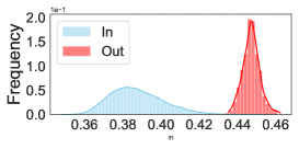
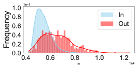
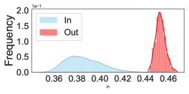
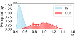
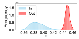
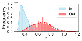
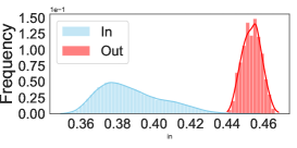
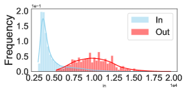
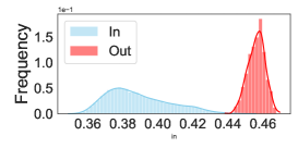
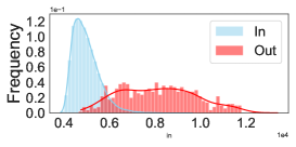
Fig. 8: OOD detection score histogram when the IN-DS is IMDB OUT-DS is TREC for various checkpoints. Left column corresponds to TRUSTED while the right column corresponds to Mahalanobis distance.

C.2 Analysis Per IN-Dataset

In Fig. 9, we conduct a dynamical analysis per IN-DS. We observe a variation of performance (e.g., up to 10 AUROC points for sst2 for $D_{\mathrm{M}}$) while probing accross time.
Takeaways: Although our method achieves strong results a key dimension when deploying OOD detection methods is to carefully select the checkpoints when learning the classifier.

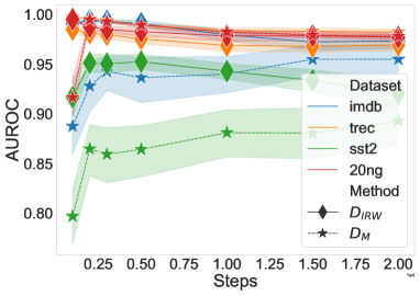
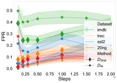
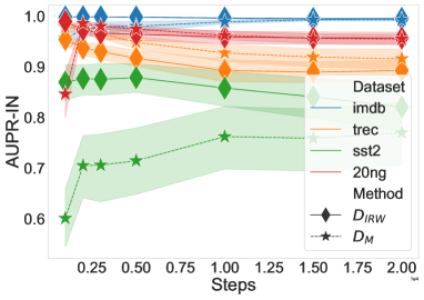
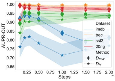
Fig. 9: OOD performance across different checkpoints for the different IN-DS.

C.3 Impact of the pretrained encoder

In Fig. 10, we report the results of the dynamical analysis and study the influence of the encoder choice on the detection performance.
Takeaways Although, TRUSTED achieves strong results on a large number of configurations. We observe different behaviours while considering different success criterion or different pretrained models. For examples, on BERT and DIS., TRUSTED is uniformly better across checkpoints when considering Fig. 10. For ROB., TRUSTED is not better on all metrics on last checkpoint (e.g., 20k).

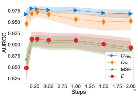
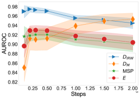
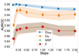
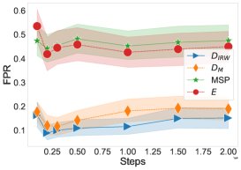
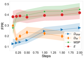
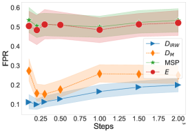
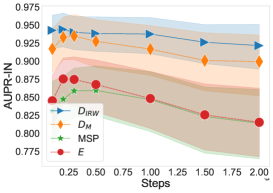
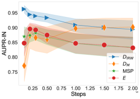
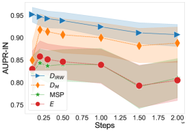
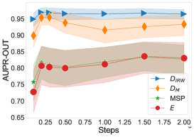
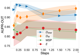
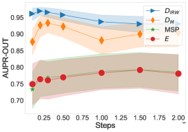
Fig. 10: OOD performance of the four considers methods across different checkpoints for the different pretrained models.

C.4 All Combinations

For completeness of the paper, we report all the results of the dynamical analysis for all considered combinations in this section (see Fig. 11 Fig. 12 Fig. 13 Fig. 14). We believe this will allow the curious reader to gain more intuition and draw nuanced conclusions from our experiments.

C.5 Futur works

Futur works include testing our method on different settings such as sequence generation, multimodal learning or automatic evaluation [21, 36, 53, 101, 43, 28, 15].

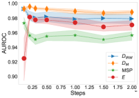
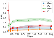
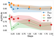
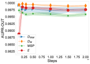
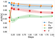
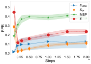
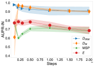
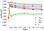
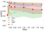
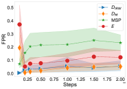
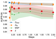
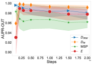
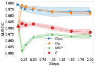
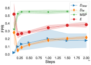
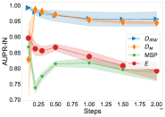
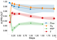
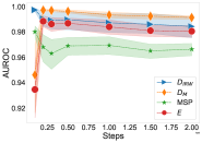
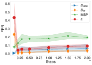
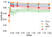
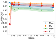
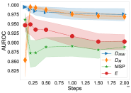
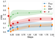
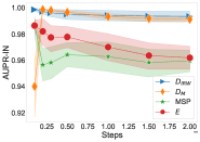
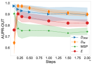
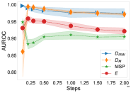
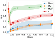
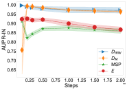
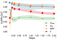
Fig. 11: OOD performance of the four considers methods across different OUT-DS for 20NG. Results are aggregated per pretrained models.

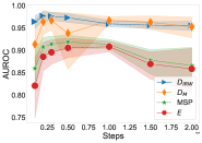
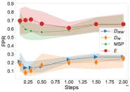
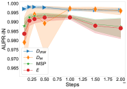
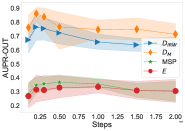
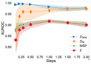
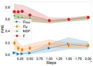
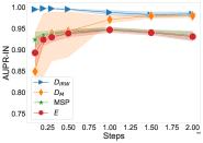
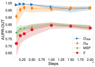
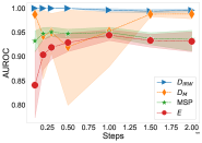
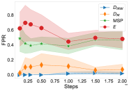
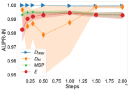
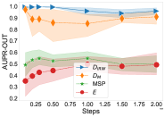
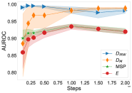
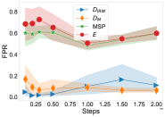
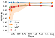
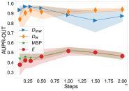
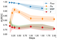
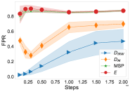
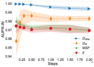
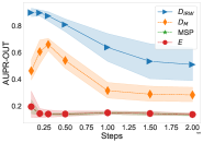
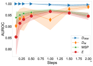
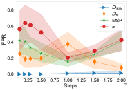
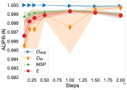
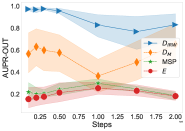
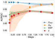
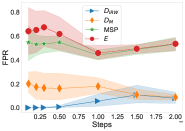
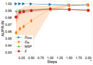
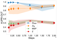
Fig. 12: OOD performance of the four considers methods across different OUT-DS for IMDB. Results are aggregated per pretrained models.

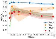
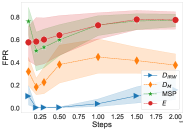
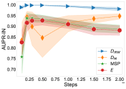
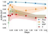
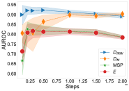
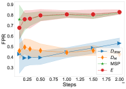
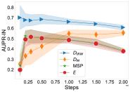
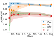
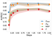
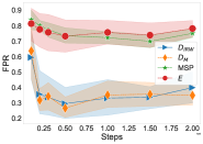
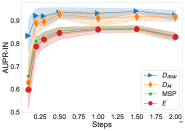
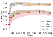
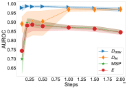
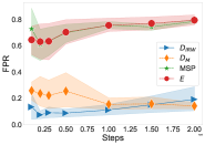
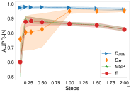
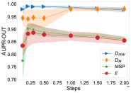
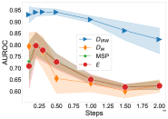
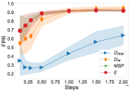
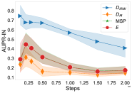
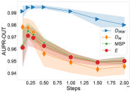
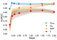
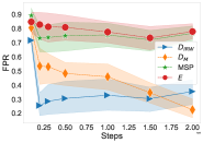
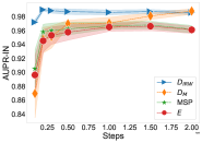
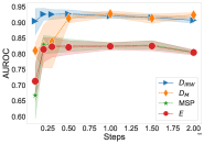
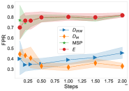
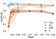
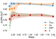
Fig. 13: OOD performance of the four considers methods across different OUT-DS for SST2. Results are aggregated per pretrained models.

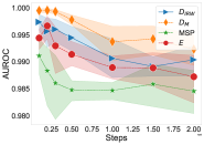
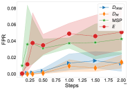
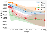
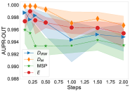
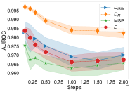
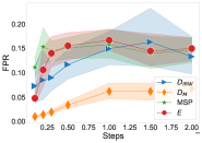
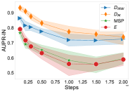
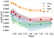
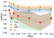
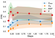
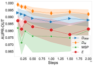
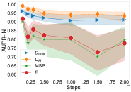
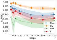
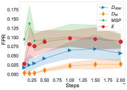
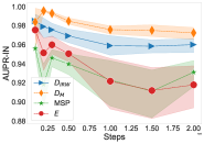
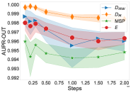
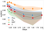
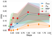
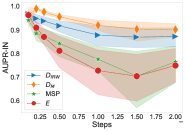
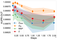
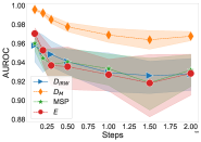
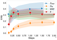
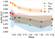
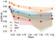
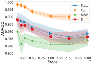
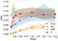
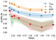
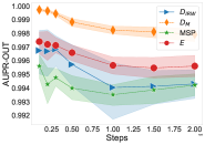
Fig. 14: OOD performance of the four considers methods across different OUT-DS for TREC. Results are aggregated per pretrained models.

References

- Ahmed and Courville [2020] Faruk Ahmed and Aaron Courville. Detecting semantic anomalies. In Proceedings of the AAAI Conference on Artificial Intelligence, volume 34, pages 3154–3162, 2020.
- Arora et al. [2021] Udit Arora, William Huang, and He He. Types of out-of-distribution texts and how to detect them. arXiv preprint arXiv:2109.06827, 2021.
- Bae et al. [2018] Ho Bae, Jaehee Jang, Dahuin Jung, Hyemi Jang, Heonseok Ha, Hyungyu Lee, and Sungroh Yoon. Security and privacy issues in deep learning. arXiv preprint arXiv:1807.11655, 2018.
- Barakat and Bianchi [2018] Anas Barakat and Pascal Bianchi. Convergence and dynamical behavior of the adam algorithm for non-convex stochastic optimization. arXiv preprint arXiv:1810.02263, 2018.
- Barocas et al. [2017] Solon Barocas, Moritz Hardt, and Arvind Narayanan. Fairness in machine learning. Nips tutorial, 1:2, 2017.
- Barreno et al. [2010] Marco Barreno, Blaine Nelson, Anthony D Joseph, and J Doug Tygar. The security of machine learning. Machine Learning, 81(2):121–148, 2010.
- Bhatia et al. [2016] K. Bhatia, K. Dahiya, H. Jain, P. Kar, A. Mittal, Y. Prabhu, and M. Varma. The extreme classification repository: Multi-label datasets and code, 2016. URL http://manikvarma.org/downloads/XC/XMLRepository.html.
- Bojar et al. [2016] Ondrej Bojar, Rajen Chatterjee, Christian Federmann, Yvette Graham, Barry Haddow, Matthias Huck, Antonio Jimeno Yepes, Philipp Koehn, Varvara Logacheva, Christof Monz, Matteo Negri, Aurelie Neveol, Mariana Neves, Martin Popel, Matt Post, Raphael Rubino, Carolina Scarton, Lucia Specia, Marco Turchi, Karin Verspoor, and Marcos Zampieri. Findings of the 2016 conference on machine translation. In Proceedings of the First Conference on Machine Translation, pages 131–198, Berlin, Germany, August 2016. Association for Computational Linguistics. URL http://www.aclweb.org/anthology/W/W16/W16-2301.
- Bommasani et al. [2021] Rishi Bommasani, Drew A Hudson, Ehsan Adeli, Russ Altman, Simran Arora, Sydney von Arx, Michael S Bernstein, Jeannette Bohg, Antoine Bosselut, Emma Brunskill, et al. On the opportunities and risks of foundation models. arXiv preprint arXiv:2108.07258, 2021.
- Bradley [1997] Andrew P Bradley. The use of the area under the roc curve in the evaluation of machine learning algorithms. Pattern recognition, 30(7):1145–1159, 1997.
- Bulusu et al. [2020] Saikiran Bulusu, Bhavya Kailkhura, Bo Li, Pramod K Varshney, and Dawn Song. Anomalous example detection in deep learning: A survey. IEEE Access, 8:132330–132347, 2020.
- Burger and Ferro [2005] J. Burger and L. Ferro. Generating an entailment corpus from news headlines. In Proceedings of the ACL Workshop on Empirical Modeling of Semantic Equivalence and Entailment, pages 49–54. Association for Computational Linguistics, 2005.
- Burkart and Huber [2021] Nadia Burkart and Marco F Huber. A survey on the explainability of supervised machine learning. Journal of Artificial Intelligence Research, 70:245–317, 2021.
- Callaway et al. [2021] Ewen Callaway et al. Deepmind’s ai predicts structures for a vast trove of proteins. Nature, 595(7869):635–635, 2021.
- Chapuis et al. [2020] Emile Chapuis, Pierre Colombo, Matteo Manica, Matthieu Labeau, and Chloe Clavel. Hierarchical pre-training for sequence labelling in spoken dialog. arXiv preprint arXiv:2009.11152, 2020.
- Chen et al. [2015] Bo Chen, Kai Ming Ting, Takashi Washio, and Gholamreza Haffari. Half-space mass: a maximally robust and efficient data depth method. Machine Learning, 100(2):677–699, 2015.
- Chen et al. [2021] Jiahao Chen, Victor Storchan, and Eren Kurshan. Beyond fairness metrics: Roadblocks and challenges for ethical ai in practice. arXiv preprint arXiv:2108.06217, 2021.
- Chhun et al. [2022] Cyril Chhun, Pierre Colombo, Chloé Clavel, and Fabian M Suchanek. Of human criteria and automatic metrics: A benchmark of the evaluation of story generation. arXiv preprint arXiv:2208.11646, 2022.
- Choi et al. [2018] Hyunsun Choi, Eric Jang, and Alexander A Alemi. Waic, but why? generative ensembles for robust anomaly detection. arXiv preprint arXiv:1810.01392, 2018.
- Colombo [2021] Pierre Colombo. Learning to represent and generate text using information measures. PhD thesis, Institut polytechnique de Paris, 2021.
- Colombo et al. [2019] Pierre Colombo, Wojciech Witon, Ashutosh Modi, James Kennedy, and Mubbasir Kapadia. Affect-driven dialog generation. arXiv preprint arXiv:1904.02793, 2019.
- Colombo et al. [2021a] Pierre Colombo, Emile Chapuis, Matthieu Labeau, and Chloé Clavel. Code-switched inspired losses for spoken dialog representations. In Proceedings of the 2021 Conference on Empirical Methods in Natural Language Processing, pages 8320–8337, 2021a.
- Colombo et al. [2021b] Pierre Colombo, Emile Chapuis, Matthieu Labeau, and Chloe Clavel. Improving multimodal fusion via mutual dependency maximisation. arXiv preprint arXiv:2109.00922, 2021b.
- Colombo et al. [2021c] Pierre Colombo, Chloe Clave, and Pablo Piantanida. Infolm: A new metric to evaluate summarization & data2text generation. arXiv preprint arXiv:2112.01589, 2021c.
- Colombo et al. [2021d] Pierre Colombo, Chloe Clavel, and Pablo Piantanida. A novel estimator of mutual information for learning to disentangle textual representations. arXiv preprint arXiv:2105.02685, 2021d.
- Colombo et al. [2021e] Pierre Colombo, Guillaume Staerman, Chloé Clavel, and Pablo Piantanida. Automatic text evaluation through the lens of Wasserstein barycenters. In Proceedings of the 2021 Conference on Empirical Methods in Natural Language Processing, pages 10450–10466, Online and Punta Cana, Dominican Republic, November 2021e. Association for Computational Linguistics. doi: 10.18653/v1/2021.emnlp-main.817. URL https://aclanthology.org/2021.emnlp-main.817.
- Colombo et al. [2021f] Pierre Colombo, Chouchang Yang, Giovanna Varni, and Chloé Clavel. Beam search with bidirectional strategies for neural response generation. arXiv preprint arXiv:2110.03389, 2021f.
- Colombo et al. [2022a] Pierre Colombo, Nathan Noiry, Ekhine Irurozki, and Stéphan Clémençon. What are the best systems? new perspectives on nlp benchmarking. arXiv preprint arXiv:2202.03799, 2022a.
- Colombo et al. [2022b] Pierre Colombo, Guillaume Staerman, Nathan Noiry, and Pablo Piantanida. Learning disentangled textual representations via statistical measures of similarity. arXiv preprint arXiv:2205.03589, 2022b.
- D’Amour et al. [2020] Alexander D’Amour, Katherine Heller, Dan Moldovan, Ben Adlam, Babak Alipanahi, Alex Beutel, Christina Chen, Jonathan Deaton, Jacob Eisenstein, Matthew D Hoffman, et al. Underspecification presents challenges for credibility in modern machine learning. arXiv preprint arXiv:2011.03395, 2020.
- Davis and Goadrich [2006] Jesse Davis and Mark Goadrich. The relationship between precision-recall and roc curves. In Proceedings of the 23rd international conference on Machine learning, pages 233–240, 2006.
- De Maesschalck et al. [2000] Roy De Maesschalck, Delphine Jouan-Rimbaud, and Désiré L Massart. The mahalanobis distance. Chemometrics and intelligent laboratory systems, 50(1):1–18, 2000.
- de Montjoye et al. [2017] Yves-Alexandre de Montjoye, Ali Farzanehfar, Julien Hendrickx, and Luc Rocher. Solving artificial intelligence’s privacy problem. Field Actions Science Reports, 17(1):80–83, 2017.
- Devlin et al. [2018] Jacob Devlin, Ming-Wei Chang, Kenton Lee, and Kristina Toutanova. Bert: Pre-training of deep bidirectional transformers for language understanding. arXiv preprint arXiv:1810.04805, 2018.
- Devlin et al. [2019] Jacob Devlin, Ming-Wei Chang, Kenton Lee, and Kristina Toutanova. BERT: Pre-training of deep bidirectional transformers for language understanding. In Proceedings of the 2019 Conference of the North American Chapter of the Association for Computational Linguistics: Human Language Technologies, Volume 1 (Long and Short Papers), pages 4171–4186, Minneapolis, Minnesota, June 2019. Association for Computational Linguistics. doi: 10.18653/v1/N19-1423. URL https://aclanthology.org/N19-1423.
- Dinkar et al. [2020] Tanvi Dinkar, Pierre Colombo, Matthieu Labeau, and Chloé Clavel. The importance of fillers for text representations of speech transcripts. arXiv preprint arXiv:2009.11340, 2020.
- Donoho and Gasko [1992] David L. Donoho and Miriam Gasko. Breakdown properties of location estimates based on half space depth and projected outlyingness. The Annals of Statistics, 20:1803–1827, 1992.
- Dror et al. [2019] Rotem Dror, Segev Shlomov, and Roi Reichart. Deep dominance-how to properly compare deep neural models. In Proceedings of the 57th Annual Meeting of the Association for Computational Linguistics, pages 2773–2785, 2019.
- Dyckerhoff and Mozharovskyi [2016] Rainer Dyckerhoff and Pavlo Mozharovskyi. Exact computation of the halfspace depth. Computational Statistics & Data Analysis, 98:19–30, 2016.
- Elliott et al. [2016] Desmond Elliott, Stella Frank, Khalil Sima’an, and Lucia Specia. Multi30K: Multilingual English-German image descriptions. In Proceedings of the 5th Workshop on Vision and Language, pages 70–74, Berlin, Germany, August 2016. Association for Computational Linguistics. doi: 10.18653/v1/W16-3210. URL https://aclanthology.org/W16-3210.
- Faria [2018] José M Faria. Machine learning safety: An overview. In Proceedings of the 26th Safety-Critical Systems Symposium, York, UK, pages 6–8, 2018.
- Gangal et al. [2020] Varun Gangal, Abhinav Arora, Arash Einolghozati, and Sonal Gupta. Likelihood ratios and generative classifiers for unsupervised out-of-domain detection in task oriented dialog. In Proceedings of the AAAI Conference on Artificial Intelligence, volume 34, pages 7764–7771, 2020.
- Garcia et al. [2019] Alexandre Garcia, Pierre Colombo, Slim Essid, Florence d’Alché Buc, and Chloé Clavel. From the token to the review: A hierarchical multimodal approach to opinion mining. arXiv preprint arXiv:1908.11216, 2019.
- Gomes et al. [2022] Eduardo Dadalto Camara Gomes, Florence Alberge, Pierre Duhamel, and Pablo Piantanida. Igeood: An information geometry approach to out-of-distribution detection. arXiv preprint arXiv:2203.07798, 2022.
- Hallin et al. [2010] Marc Hallin, Davy Paindaveine, and Miroslav Šiman. Multivariate quantiles and multiple-output regression quantiles: From l1 optimization to halfspace depth. The Annals of Statistics, 38(2):635–669, 04 2010.
- Hardy et al. [1952] Godfrey Harold Hardy, John Edensor Littlewood, George Pólya, György Pólya, et al. Inequalities. Cambridge university press, 1952.
- Hendrycks and Gimpel [2016] Dan Hendrycks and Kevin Gimpel. A baseline for detecting misclassified and out-of-distribution examples in neural networks. arXiv preprint arXiv:1610.02136, 2016.
- Hendrycks et al. [2018] Dan Hendrycks, Mantas Mazeika, and Thomas Dietterich. Deep anomaly detection with outlier exposure. arXiv preprint arXiv:1812.04606, 2018.
- Hendrycks et al. [2020] Dan Hendrycks, Xiaoyuan Liu, Eric Wallace, Adam Dziedzic, Rishabh Krishnan, and Dawn Song. Pretrained transformers improve out-of-distribution robustness. arXiv preprint arXiv:2004.06100, 2020.
- Hendrycks et al. [2021] Dan Hendrycks, Nicholas Carlini, John Schulman, and Jacob Steinhardt. Unsolved problems in ml safety. arXiv preprint arXiv:2109.13916, 2021.
- Hickl et al. [2006] A. Hickl, J. Williams, J. Bensley, K. Roberts, B. Rink, and Y. Shi. Recognizing textual entailment with lcc’s groundhog system. In Proceedings of the Second PASCAL Challenges Workshop, 2006.
- Hsu et al. [2020] Yen-Chang Hsu, Yilin Shen, Hongxia Jin, and Zsolt Kira. Generalized odin: Detecting out-of-distribution image without learning from out-of-distribution data. 2020 IEEE/CVF Conference on Computer Vision and Pattern Recognition (CVPR), pages 10948–10957, 2020.
- Jalalzai et al. [2020] Hamid Jalalzai, Pierre Colombo, Chloé Clavel, Éric Gaussier, Giovanna Varni, Emmanuel Vignon, and Anne Sabourin. Heavy-tailed representations, text polarity classification & data augmentation. Advances in Neural Information Processing Systems, 33:4295–4307, 2020.
- Joachims [1996] Thorsten Joachims. A probabilistic analysis of the rocchio algorithm with tfidf for text categorization. Technical report, Carnegie-mellon univ pittsburgh pa dept of computer science, 1996.
- Kingma and Ba [2014] Diederik P Kingma and Jimmy Ba. Adam: A method for stochastic optimization. arXiv preprint arXiv:1412.6980, 2014.
- Koshevoy and Mosler [1997] Gleb A. Koshevoy and Karl Mosler. Zonoid trimming for multivariate distributions. The Annals of Statistics, 25(5):1998–2017, 10 1997.
- Kurshan et al. [2020] Eren Kurshan, Hongda Shen, and Jiahao Chen. Towards self-regulating ai: Challenges and opportunities of ai model governance in financial services. In Proceedings of the First ACM International Conference on AI in Finance, pages 1–8, 2020.
- Lee et al. [2018] Kimin Lee, Kibok Lee, Honglak Lee, and Jinwoo Shin. A simple unified framework for detecting out-of-distribution samples and adversarial attacks. Advances in neural information processing systems, 31, 2018.
- Levinson et al. [2011] Jesse Levinson, Jake Askeland, Jan Becker, Jennifer Dolson, David Held, Soeren Kammel, J Zico Kolter, Dirk Langer, Oliver Pink, Vaughan Pratt, et al. Towards fully autonomous driving: Systems and algorithms. In 2011 IEEE intelligent vehicles symposium (IV), pages 163–168. IEEE, 2011.
- Li et al. [2021] Xiaoya Li, Jiwei Li, Xiaofei Sun, Chun Fan, Tianwei Zhang, Fei Wu, Yuxian Meng, and Jun Zhang. folden: -fold ensemble for out-of-distribution detection. arXiv preprint arXiv:2108.12731, 2021.
- Li and Roth [2002] Xin Li and Dan Roth. Learning question classifiers. In COLING 2002: The 19th International Conference on Computational Linguistics, 2002. URL https://aclanthology.org/C02-1150.
- Liang et al. [2018] Shiyu Liang, Yixuan Li, and R. Srikant. Enhancing the reliability of out-of-distribution image detection in neural networks. In International Conference on Learning Representations, 2018. URL https://openreview.net/forum?id=H1VGkIxRZ.
- Linardatos et al. [2020] Pantelis Linardatos, Vasilis Papastefanopoulos, and Sotiris Kotsiantis. Explainable ai: A review of machine learning interpretability methods. Entropy, 23(1):18, 2020.
- Liu et al. [2021] Bo Liu, Ming Ding, Sina Shaham, Wenny Rahayu, Farhad Farokhi, and Zihuai Lin. When machine learning meets privacy: A survey and outlook. ACM Computing Surveys (CSUR), 54(2):1–36, 2021.
- Liu [1990] Regina Y. Liu. On a notion of data depth based on random simplices. The Annals of Statistics, 18(1):405–414, 1990.
- Liu [1992] Regina Y. Liu. Data depth and multivariate rank tests, pages 279–294. 1992.
- Liu et al. [2020] Weitang Liu, Xiaoyun Wang, John Owens, and Yixuan Li. Energy-based out-of-distribution detection. Advances in Neural Information Processing Systems, 2020.
- Liu et al. [2019] Yinhan Liu, Myle Ott, Naman Goyal, Jingfei Du, Mandar Joshi, Danqi Chen, Omer Levy, Mike Lewis, Luke Zettlemoyer, and Veselin Stoyanov. Roberta: A robustly optimized bert pretraining approach. arXiv preprint arXiv:1907.11692, 2019.
- Loshchilov and Hutter [2017] Ilya Loshchilov and Frank Hutter. Decoupled weight decay regularization. arXiv preprint arXiv:1711.05101, 2017.
- Maas et al. [2011] Andrew L. Maas, Raymond E. Daly, Peter T. Pham, Dan Huang, Andrew Y. Ng, and Christopher Potts. Learning word vectors for sentiment analysis. In Proceedings of the 49th Annual Meeting of the Association for Computational Linguistics: Human Language Technologies, pages 142–150, Portland, Oregon, USA, June 2011. Association for Computational Linguistics. URL https://aclanthology.org/P11-1015.
- Mahalanobis et al. [1936] Prasanta Chandra Mahalanobis et al. On the generalised distance in statistics. In Proceedings of the National Institute of Sciences of India, volume 2, pages 49–55, 1936.
- Mehrabi et al. [2021] Ninareh Mehrabi, Fred Morstatter, Nripsuta Saxena, Kristina Lerman, and Aram Galstyan. A survey on bias and fairness in machine learning. ACM Computing Surveys (CSUR), 54(6):1–35, 2021.
- Nagy et al. [2020] Stanislav Nagy, Rainer Dyckerhoff, and Pavlo Mozharovskyi. Uniform convergence rates for the approximated halfspace and projection depth. Electronic Journal of Statistics, 14(2):3939–3975, 2020.
- Pichler et al. [2022] Georg Pichler, Pierre Jean A Colombo, Malik Boudiaf, Günther Koliander, and Pablo Piantanida. A differential entropy estimator for training neural networks. In International Conference on Machine Learning, pages 17691–17715. PMLR, 2022.
- Podolskiy et al. [2021] Alexander Podolskiy, Dmitry Lipin, Andrey Bout, Ekaterina Artemova, and Irina Piontkovskaya. Revisiting mahalanobis distance for transformer-based out-of-domain detection. arXiv preprint arXiv:2101.03778, 2021.
- Ramsay et al. [2019] Kelly Ramsay, Stéphane Durocher, and Alexandre Leblanc. Integrated rank-weighted depth. Journal of Multivariate Analysis, 173:51–69, 2019.
- Ramsundar et al. [2015] Bharath Ramsundar, Steven Kearnes, Patrick Riley, Dale Webster, David Konerding, and Vijay Pande. Massively multitask networks for drug discovery. arXiv preprint arXiv:1502.02072, 2015.
- Ren et al. [2019] Jie Ren, Peter J Liu, Emily Fertig, Jasper Snoek, Ryan Poplin, Mark A DePristo, Joshua V Dillon, and Balaji Lakshminarayanan. Likelihood ratios for out-of-distribution detection. arXiv preprint arXiv:1906.02845, 2019.
- Rousseeuw and Hubert [1999] Peter J. Rousseeuw and Mia Hubert. Regression depth. Journal of the American Statistical Association, 94(446):388–402, 1999.
- Rousseeuw and Hubert [2018] Peter J. Rousseeuw and Mia Hubert. Anomaly detection by robust statistics. Wiley Interdisciplinary Reviews: Data Mining and Knowledge Discovery, 8(2):e1236, 2018.
- Rousseeuw and Struyf [1998] Peter J. Rousseeuw and Anja Struyf. Computing location depth and regression depth in higher dimensions. Statistics and Computing, 8(3):193–203, 1998.
- Rücklé et al. [2018] Andreas Rücklé, Steffen Eger, Maxime Peyrard, and Iryna Gurevych. Concatenated power mean word embeddings as universal cross-lingual sentence representations. arXiv preprint arXiv:1803.01400, 2018.
- Sanh et al. [2019] Victor Sanh, Lysandre Debut, Julien Chaumond, and Thomas Wolf. Distilbert, a distilled version of bert: smaller, faster, cheaper and lighter. arXiv preprint arXiv:1910.01108, 2019.
- Sastry and Oore [2020a] Chandramouli Shama Sastry and Sageev Oore. Detecting out-of-distribution examples with Gram matrices. In Hal Daumé III and Aarti Singh, editors, Proceedings of the 37th International Conference on Machine Learning, volume 119 of Proceedings of Machine Learning Research, pages 8491–8501. PMLR, 13–18 Jul 2020a. URL https://proceedings.mlr.press/v119/sastry20a.html.
- Sastry and Oore [2020b] Chandramouli Shama Sastry and Sageev Oore. Detecting out-of-distribution examples with gram matrices. In International Conference on Machine Learning, pages 8491–8501. PMLR, 2020b.
- Sellam et al. [2021] Thibault Sellam, Steve Yadlowsky, Jason Wei, Naomi Saphra, Alexander D’Amour, Tal Linzen, Jasmijn Bastings, Iulia Turc, Jacob Eisenstein, Dipanjan Das, et al. The multiberts: Bert reproductions for robustness analysis. arXiv preprint arXiv:2106.16163, 2021.
- Serfling [2006] Robert Serfling. Depth functions in nonparametric multivariate inference. DIMACS Series in Discrete Mathematics and Theoretical Computer Science, 72, 2006.
- Socher et al. [2013] Richard Socher, Alex Perelygin, Jean Wu, Jason Chuang, Christopher D. Manning, Andrew Ng, and Christopher Potts. Recursive deep models for semantic compositionality over a sentiment treebank. In Proceedings of the 2013 Conference on Empirical Methods in Natural Language Processing, pages 1631–1642, Seattle, Washington, USA, October 2013. Association for Computational Linguistics. URL https://aclanthology.org/D13-1170.
- Srivastava et al. [2014] Nitish Srivastava, Geoffrey Hinton, Alex Krizhevsky, Ilya Sutskever, and Ruslan Salakhutdinov. Dropout: a simple way to prevent neural networks from overfitting. The journal of machine learning research, 15(1):1929–1958, 2014.
- Staerman [2022] Guillaume Staerman. Functional anomaly detection and robust estimation. PhD thesis, Institut polytechnique de Paris, 2022.
- Staerman et al. [2019] Guillaume Staerman, Pavlo Mozharovskyi, Stéphan Clémençon, and Florence d’Alché Buc. Functional isolation forest. In Proceedings of The Eleventh Asian Conference on Machine Learning, pages 332–347, 2019.
- Staerman et al. [2020] Guillaume Staerman, Pavlo Mozharovskyi, and Stéphan Clémençon. The area of the convex hull of sampled curves: a robust functional statistical depth measure. In Proceedings of the 23nd International Conference on Artificial Intelligence and Statistics (AISTATS 2020), volume 108, pages 570–579, 2020.
- Staerman et al. [2021a] Guillaume Staerman, Pavlo Mozharovskyi, Stéphan Clémençon, and Florence d’Alché Buc. A pseudo-metric between probability distributions based on depth-trimmed regions. arXiv preprint arXiv:2103.12711, 2021a.
- Staerman et al. [2021b] Guillaume Staerman, Pavlo Mozharovskyi, and Stéphan Clémençon. Affine-invariant integrated rank-weighted depth: Definition, properties and finite sample analysis. arXiv preprint arXiv:2106.11068, 2021b.
- Staerman et al. [2021c] Guillaume Staerman, Pavlo Mozharovskyi, Pierre Colombo, Stéphan Clémençon, and Florence d’Alché Buc. A pseudo-metric between probability distributions based on depth-trimmed regions. arXiv preprint arXiv:2103.12711, 2021c.
- Staerman et al. [2022] Guillaume Staerman, Eric Adjakossa, Pavlo Mozharovskyi, Vera Hofer, Jayant Sen Gupta, and Stephan Clémençon. Functional anomaly detection: a benchmark study. arXiv preprint arXiv:2201.05115, 2022.
- Tukey [1975] John W. Tukey. Mathematics and the picturing of data. In R.D. James, editor, Proceedings of the International Congress of Mathematicians, volume 2, pages 523–531. Canadian Mathematical Congress, 1975.
- Wang et al. [2022] Hongyu Wang, Shuming Ma, Li Dong, Shaohan Huang, Dongdong Zhang, and Furu Wei. Deepnet: Scaling transformers to 1,000 layers. arXiv preprint arXiv:2203.00555, 2022.
- Williams et al. [2018] Adina Williams, Nikita Nangia, and Samuel Bowman. A broad-coverage challenge corpus for sentence understanding through inference. In Proceedings of the 2018 Conference of the North American Chapter of the Association for Computational Linguistics: Human Language Technologies, Volume 1 (Long Papers), pages 1112–1122, New Orleans, Louisiana, June 2018. Association for Computational Linguistics. doi: 10.18653/v1/N18-1101. URL https://aclanthology.org/N18-1101.
- Winkens et al. [2020] Jim Winkens, Rudy Bunel, Abhijit Guha Roy, Robert Stanforth, Vivek Natarajan, Joseph R. Ledsam, Patricia MacWilliams, Pushmeet Kohli, Alan Karthikesalingam, Simon A. A. Kohl, taylan. cemgil, S. M. Ali Eslami, and Olaf Ronneberger. Contrastive training for improved out-of-distribution detection. ArXiv, abs/2007.05566, 2020.
- Witon et al. [2018] Wojciech Witon, Pierre Colombo, Ashutosh Modi, and Mubbasir Kapadia. Disney at iest 2018: Predicting emotions using an ensemble. In Proceedings of the 9th Workshop on Computational Approaches to Subjectivity, Sentiment and Social Media Analysis, pages 248–253, 2018.
- Zhong et al. [2021] Ruiqi Zhong, Dhruba Ghosh, Dan Klein, and Jacob Steinhardt. Are larger pretrained language models uniformly better? comparing performance at the instance level. arXiv preprint arXiv:2105.06020, 2021.
- Zhou et al. [2021] Wenxuan Zhou, Fangyu Liu, and Muhao Chen. Contrastive out-of-distribution detection for pretrained transformers. arXiv preprint arXiv:2104.08812, 2021.
- Zuo and Serfling [2000] Yijun Zuo and Robert Serfling. General notions of statistical depth function. The Annals of Statistics, 28(2):461–482, 2000.