Evaluating Search-Based Software Microbenchmark Prioritization

Abstract

Ensuring that software performance does not degrade after a code change is paramount. A solution is to regularly execute software microbenchmarks, a performance testing technique similar to (functional) unit tests, which, however, often becomes infeasible due to extensive runtimes. To address that challenge, research has investigated regression testing techniques, such as test case prioritization (TCP), which reorder the execution within a microbenchmark suite to detect larger performance changes sooner. Such techniques are either designed for unit tests and perform sub-par on microbenchmarks or require complex performance models, drastically reducing their potential application. In this paper, we empirically evaluate single- and multi-objective search-based microbenchmark prioritization techniques to understand whether they are more effective and efficient than greedy, coverage-based techniques. For this, we devise three search objectives, i.e., coverage to maximize, coverage overlap to minimize, and historical performance change detection to maximize. We find that search algorithms (SAs) are only competitive with but do not outperform the best greedy, coverage-based baselines. However, a simple greedy technique utilizing solely the performance change history (without coverage information) is equally or more effective than the best coverage-based techniques while being considerably more efficient, with a runtime overhead of less than $1$%.These results show that simple, non-coverage-based techniques are a better fit for microbenchmarks than complex coverage-based techniques.

1 Introduction

Regression testing comprises effective techniques for revealing faults in continuously evolving software systems [35], e.g., as part of continuous integration (CI) [25, 62, 33, 26]. To detect performance problems, particularly, in software libraries and frameworks, microbenchmarks are the predominantly used performance testing technique, similar to unit tests for functional testing [76]. However, their extensive runtimes inhibit their adoption in CI [40, 76, 51, 54]. In our previous work [54], we found that $15$% of the Java Microbenchmark Harness (JMH) suites on GitHub run longer than three hours and $3$% longer than $12$ hours. Therefore, it is inevitable to employ performance regression testing techniques, such as software microbenchmark prioritization (SMBP) (test case prioritization (TCP) on software microbenchmarks), to capture important performance changes as early as possible.

Catching performance problems early is crucial for industry. Meta mentioned that performance regression testing is worth investigating [2], and MongoDB has created a sophisticated solution to run benchmarks as part of CI [13]. Though academic research on microbenchmarks has recently gained attention [59, 76, 51, 15, 42], performance regression testing on microbenchmark-level is still scarce, mostly focusing on regression test selection (RTS) for performance tests [17, 3, 4, 11]. Mostafa et al. [67] are the first to apply SMBP, introducing a technique based on a complex performance-impact model, which is, however, only suited for collection-intensive software and non-trivial to apply. In our previous work [56], we perform a large-scale study of coverage-based, greedy heuristics for SMBP, inspired by TCP [73, 24, 64], and found that the studied techniques are not nearly as effective on microbenchmarks as on unit tests and impose a relatively large runtime overhead of $17$%.

A promising approach is search-based techniques, which are highly effective for various software engineering optimization problems [1, 84, 29, 5, 60, 41, 27, 65, 22]. Motivated by these successes, in this paper, we define search-based software microbenchmark prioritization (SBSMBP) problems and solve them with single-objective search algorithms (SAs) and multi-objective evolutionary algorithms (MOEAs), with (up to) three objectives: (1) coverage (C), (2) coverage overlap among benchmarks (CO), and (3) historical performance change size (CH). Moreover, we define new Greedy SMBP techniques based on each of the three objectives as well as their combination (C-CO-CH).

We evaluate the SBSMBP (two single-objective SAs and six MOEAs) and Greedy SMBP techniques on $10$ JMH suites having $1,829$ distinct microbenchmarks with $6,460$ distinct parameterizations across $161$ versions, regarding (1) effectiveness measured by the average percentage of fault-detection on performance (APFD-P); and (2) efficiency measured as the runtime overhead. The study compares the SBSMBP and Greedy SMBP techniques to two greedy, coverage-based baselines, i.e., Total and Additional [67, 56].

The results show that the best SBSMBP technique, i.e., the single-objective Generational Genetic Algorithm (GA) combining the three objectives with weighted-sum (GA C-CO-CH), performs competitively with the best greedy baseline, i.e., Total. However, it does not outperform Total regarding effectiveness, with both having an overall median APFD-P of $0.60$, while only adding a minor additional overhead of $1$% compared to below $1$% for Total. The best MOEA is Multi-Objective Cellular Genetic Algorithm (MOCell), which is not as effective as GA C-CO-CH and Total, with an overall median APFD-P of $0.58$. Surprisingly, the Greedy technique that relies only on the historical performance change size (i.e., Greedy CH) performs better than Total regarding median APFD-P of $0.65$. Statistically, the best Greedy and SBSMBP techniques perform equally to Total, regarding effectiveness. However, Greedy CH is more effective than Total for one of the studied projects and never worse, while having a significantly lower overhead of $1$% consistently across the studied projects, whereas the coverage-based techniques have overheads ranging between $8$% and $105$% across the projects and $17$% on average.

These results tell that the Greedy technique relying solely on the performance change history (CH) performs the best, and it is arguably the simplest to implement. Hence, we recommend practitioners to employ the Greedy CH technique to achieve consistently earlier performance change detection, e.g., as part of CI, and researchers to investigate non-coverage-based SMBP techniques in the future.

To summarize, the main contributions of this paper are:

• the first paper to describe SMBP with search (SBSMBP);

• three search objectives (two of which are novel) to use in SMBP algorithms;

• an experimental study showing the effectiveness and efficiency of the new Greedy SMBP and SBSMBP techniques compared to greedy baselines;

• an experimental study on the impact of change-awareness on the SMBP techniques; and

• an experimental study on the effectiveness and efficiency of two single-objective SAs and six MOEAs.

We provide all data and scripts in our replication package [58] and the SMBPs implementations in bencher v0.4.0 [52].

2 Software Microbenchmarking with JMH

Software microbenchmarking is a performance testing technique that can be seen as the equivalent of unit testing for functional testing. A software microbenchmark, microbenchmark or benchmark for short and used thereafter, measures a performance metric, usually runtime or throughput, of small code units, such as statements and methods.

The Java Microbenchmark Harness (JMH) is the de facto standard for defining and executing Java microbenchmarks. They are defined in source code with annotations, similar to JUnit. LABEL:lst:jmh shows a simplified example. A benchmark is a method annotated with @Benchmark (lines $8$–$15$), which optionally takes parameters as input, i.e., an Input object containing an instance variable annotated with @Param (lines $9$ and $17$–$21$), called the parameterization of a benchmark.

⬇

1@Fork(3)

2@Warmup(iterations = 10, time = 1, timeUnit = TimeUnit.SECONDS)

3@Measurement(iterations = 20, time = 1, timeUnit = TimeUnit.SECONDS)

4@BenchmarkMode(Mode.SampleTime)

5@OutputTimeUnit(TimeUnit.NANOSECONDS)

6public class ComputationSchedulerPerf {

7

8 @Benchmark

9 public void observeOn(Input input) {

10 LatchedObserver<Integer> o = input.newLatchedObserver();

11 input.observable

12 .observeOn(Schedulers.computation())

13 .subscribe(o);

14 o.latch.await();

15 }

16

17 @State(Scope.Thread)

18 public static class Input extends InputWithIncrementingInteger {

19 @Param({ "1", "1000" })

20 public int size;

21 }

22}

Listing 1: Modified JMH example from RxJava

As measuring performance is non-deterministic and multiple factors can influence the measurement, one has to repeatedly execute each benchmark to get reliable results. JMH executes each combination of a benchmark method and its parameterization according to a specified configuration, set through annotations on class or method level (lines $1$–$5$) or through the command line interface (CLI). Figure 1 visualizes the repeated execution of a benchmark suite. Each (parameterized) benchmark is invoked as often as possible for a defined time period (e.g., $1$s, configured on lines $2$ and $3$), called an iteration, and the measured performance metrics are reported. To get reliable results, JMH first runs a set of warmup iterations (line $2$ and “wi”) to get the system into a steady state, for which the measurements are discarded. After the warmup, JMH runs a set of measurement iterations (line $3$ and “mi”). To deal with non-determinism of the Java Virtual Machine (JVM), JMH repeats the sets of warmup and measurement iterations for a number of forks (line $1$ and “f”), each in a new JVM instance. The result of a benchmark is then the distribution of all measurement iterations (“mi”) of all forks (“f”). A microbenchmark suite usually contains many benchmarks, which JMH executes sequentially.

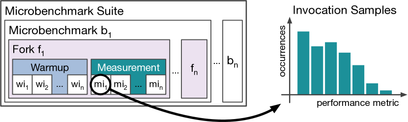
Figure 1: JMH Execution

3 Search-Based Prioritization

This section defines SBSMBP, which draws inspiration from search-based TCP [60, 41, 27, 65, 22] and greedy SMBP [56].

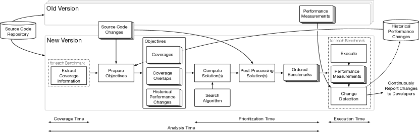
Figure 2: search-based software microbenchmark prioritization (adapted and extended from our previous work [56])

Figure 2 depicts an overview of SBSMBP. Upon a new version, the source code is retrieved from a repository. First, the coverage information is extracted for every benchmark. This is different from TCP where coverage information is retrieved during the test execution, and the TCP technique uses the coverage of the old version for ranking the test execution of the new version. This is due to unit tests being usually only executed once. Because benchmarks are executed repeatedly for rigorous measurements, SBSMBP can leverage a single execution before the measurement to extract coverage information. Based on the coverage information, historical performance changes, and source code changes (in case the technique implements change-awareness), a pre-processing stage prepares the search objectives. Then, SBSMBP employs a SA to compute a SMBP ranking (solution), i.e., ordered benchmarks. SBSMBP can be parameterized with either a single-, multi-, or many-objective SA.

The post-processing stage has two tasks. (1) Select one solution from the SA results. In the single-objective SA case there is only one solution. In the multi-objective SA case, the SA returns the Pareto front containing multiple solutions to select from [28]. (2) Adjust the benchmark order based on the source code changes, when using a change-awareness technique (see Section 4.3.4). Finally, SBSMBP executes the whole benchmark suite in the optimized order. That is, it executes each benchmark repeatedly according to performance engineering best practice [30], measures the performance and compares the measurements to the old version for change detection. The changes are then reported to the developers and stored for future versions, i.e., to compute the historical performance changes objective.

4 Experimental Study

We conduct a laboratory experiment [77] to empirically study the effectiveness and efficiency of SBSMBP.

4.1 Research Questions

We pose the following research questions (RQs):

RQ1

How effective is SBSMBP?

RQ1a

Which SBSMBP technique is most effective?

RQ1b

How do SBSMBP techniques compare to greedy techniques?

RQ1c

How does change-awareness impact effectiveness?

RQ2

How efficient is SBSMBP?

RQ1 addresses the effectiveness of SBSMBP by first investigating different SAs and objectives in RQ1a to find the most effective SBSMBP techniques, which we subsequently compare with greedy SMBP techniques in RQ1b, including the Total and Additional baselines. RQ1c assesses the impact of two source code change-aware techniques compared to the non-change-aware technique on SMBP effectiveness. Finally, RQ2 studies the runtime overhead that the SBSMBP techniques impose compared to the greedy techniques, which shows the practical feasibility.

4.2 Dataset

To perform our experimental evaluation, we require executions of (1) dedicated benchmarks (but not unit tests utilized as performance tests because their execution is not rigorous concerning performance testing and benchmarking best practice [30]); (2) full benchmark suites, as TCP/SMBP is defined by executing a full suite in a certain order [73, 74]; (3) multiple versions of the same project to perform regression testing; and (4) multiple projects to improve external validity. In addition, a rigorous performance evaluation demands high standards and compliance with the performance engineering best practice to reduce internal validity threats [30, 66]. We are only aware of one dataset that adheres to these criteria, which is from our previous work and was specifically created for SMBP [56, 57]. The dataset includes (1) JMHbenchmark suite executions, (2) dynamic coverage information on method level for these benchmarks, and (3) coverage-based, greedy baselines for TCP on benchmarks. Though there are a few papers on microbenchmarking and performance regression testing [10, 67, 17, 11, 78], no other dataset fits the above-mentioned criteria. Hence, we only select the dataset of our previous work [56, 57] for our experiment.

4.2.1 Study Objects

The dataset has $10$ open-source software (OSS) Java projects hosted on GitHub, which contain JMH suites. The projects have $59,164$ benchmarks in total and $6,460$ distinct benchmarks across $161$ versions. Distinct benchmarks are counted once across all versions they occur in. In this paper, we consider a benchmark to be the instantiation of a JMH benchmark method (annotated with @Benchmark) with concrete parameterization (using JMH parameters annotated with @Param). Table I provides an overview of these projects. Columns “Benchmarks” and “Runtime” show the arithmetic mean and standard deviation across the versions of each project, as different versions potentially have a different number of benchmarks and, hence, varying runtimes.

Table I: Study objects from the dataset [56]

Project	Versions	Benchmarks		Runtime [h]
		mean	stdev	mean	stdev
Byte Buddy	$31$	$30.74$	$\pm$ $8$	$0.26$	$\pm$ $0.069$
Eclipse Collections	$10$	$2,371.40$	$\pm$ $13$	$38.45$	$\pm$ $0.124$
JCTools	$11$	$126.91$	$\pm$ $52$	$1.15$	$\pm$ $0.481$
Jenetics	$21$	$49.24$	$\pm$ $6$	$0.42$	$\pm$ $0.053$
Log4j 2	$15$	$309.53$	$\pm$ $162$	$2.71$	$\pm$ $1.398$
Netty	$10$	$746.50$	$\pm$ $522$	$6.56$	$\pm$ $4.625$
Okio	$11$	$181.64$	$\pm$ $20$	$1.56$	$\pm$ $0.170$
RxJava	$19$	$842.63$	$\pm$ $228$	$7.81$	$\pm$ $2.113$
Xodus	$11$	$67.00$	$\pm$ $10$	$1.33$	$\pm$ $0.104$
Zipkin	$22$	$55.18$	$\pm$ $11$	$0.48$	$\pm$ $0.101$

4.2.2 Benchmark Executions and Performance Changes

We executed the benchmarks in a controlled environment for a predefined number of repetitions, following the best practice [30, 66]. The executions used a unified configuration for all the benchmarks, i.e., $10$ warmup iterations and $20$ measurement iterations of $1\text{\,}\mathrm{s}$ each. In addition, we executed the full suites for $3$ trials (note that a trial is different from a JMH fork, in that it is executed at different points in time and not back-to-back), leading to a total runtime for all the projects, versions, and repetitions of approximately $89$ days.

Based on the executions, the performance changes are computed between adjacent versions with a Monte-Carlo technique to estimate the confidence intervals of the ratio of the means. The technique is based on Kalibera and Jones [45, 46] and employs bootstrap [16] with hierarchical random resampling with replacement [71] on three levels, i.e., trial, iteration, and benchmark invocation. It uses $10,000$ bootstrap iterations [39] and a confidence level of $99$%. For this, we used the pa tool [50].

4.2.3 Coverage Information and SMBP Baselines

The dataset provides the necessary coverage information for the SBSMBP, Greedy SMBP, and greedy baseline techniques. Dynamic coverage information, i.e., method coverage, is extracted per benchmark and version with JaCoCo, by executing a benchmark once (with JMH’s single-shot mode) and injecting the JaCoCo agent. Based on these coverages, we [56] studied coverage-based, greedy SMBP techniques, particularly Total and Additional – our baselines.

4.3 Independent Variables

Our experiment investigates four independent variables: (1) the prioritization strategies, (2) the SAs employed in the SBSMBP techniques, (3) the search objectives used for solving the SBSMBP problem, and (4) the change-awareness of the technique, which are described below in detail.

4.3.1 Prioritization Strategies

The four different prioritization strategies are: (1) the coverage-based, greedy Total strategy, which ranks the benchmarks in a suite, based on their total number of covered units, from the one with the most to the one with the least; (2) the coverage-based, greedy Additional strategy, which ranks the benchmarks, based on the number of covered units not yet been considered for prioritization by previously ranked benchmarks; (3) a Greedy strategy which ranks the benchmarks according to either one or three of the search objectives; and (4) the search-based strategy described in Section 3. The strategies relying on code coverage use dynamic method coverage, aligned with our previous work [56].

The Total and Additional strategies have their roots in unit testing [73, 74], are the standard coverage-based techniques with good effectiveness [34, 64], and were recently adapted for benchmarks [67, 56]. Our experiment parameterizes Total and Additional with a benchmark granularity for both the prioritization strategy and the coverage extraction on the parameter level, which we showed to be optimal [56]. The Greedy strategy based on the search objectives uses either coverage, coverage-overlap, performance change history, or a combination of these. The parameterization of the search-based strategy is mostly concerned with the employed SA and search objectives, which are distinct independent variables of our experiment that the next sections describe.

4.3.2 search algorithms (SAs)

We study eight SAs: (1) Steepest Ascent Hill Climbing (HC), (2) Generational Genetic Algorithm (GA), (3) Indicator-Based Evolutionary Algorithm (IBEA) [85] using the hypervolume [7], (4) Multi-Objective Cellular Genetic Algorithm (MOCell) [68], (5) Non-Dominated Sorting Genetic Algorithm II (NSGAII) [19], (6) Non-Dominated Sorting Genetic Algorithm III (NSGAIII) [18], (7) Pareto Archived Evolution Strategy (PAES) [48], and (8) Strength Pareto Evolutionary Algorithm 2 (SPEA2) [86, 47]. The first two are single-objective SAs, and the other six are MOEAs. We select these to cover a wide range of algorithms that have been used in previous search-based test optimization research [82, 60, 27, 22] and are supported by jMetal [69].

Solution Encoding

A SBSMBP solution is encoded as an integer permutation, where its length corresponds to the number of benchmarks in a suite, and each element corresponds to an integer identifier mapping to a unique benchmark in that suite. We choose this encoding because the SMBP problem has the constraint that each benchmark exists exactly once in every solution. SBSMBP then executes the benchmark suite in the order of the solution.

Algorithm Parameters

Our experiment uses the same parameter settings across the SAs where possible to facilitate a fair comparison, which are also in line with previous research on multi-objective TCP [41, 61, 27, 65, 22]. The algorithm parameters are set to:

• population size: $250$;

• selection: binary tournament selection;

• crossover: PMX-Crossover with a probability $p_{c}=0.9$;

• mutation: SWAP-Mutation with a probability $p_{m}=1/n$, where $n$ is the number of benchmarks to prioritize;

• maximum number of generations: $100$; and

• maximum evaluations: population size times the maximum number of generations, i.e., $25,000$.

Note that not all SAs make use of all the parameters. Archive-based MOEAs, i.e., IBEA, MOCell, and PAES, use an archive size equal to the population size, which is in line with the papers that introduced them [85, 68, 48] and the JMetal defaults. MOCell is an exception, which requires a population size that is the power of $2$ of an integer; hence, we set MOCell’s population size to $256$, which is the closest to the population size of the other MOEAs, i.e., $250$, and its maximum number of generations to $25,600$.

HC Neighborhood

We define the neighborhood of a solution as the benchmark orderings that swap the first benchmark with each of the other benchmarks. The neighborhood size is $n-1$, where $n$ is the number of benchmarks in the suite. This definition is in line with previous research to keep HC scalable [60]. Other definitions would also be valid, e.g., swapping any two benchmarks; however, this would not scale, as for every iteration HC would need to check $\mathcal{O}(n^{2})$ neighbors.

4.3.3 Search Objectives

The ideal search objective would be the actual performance changes (faults) the benchmark suite detects upon a new release, which, however, are only known after the execution (see Section 2 for details). Hence, the search requires objectives that are good proxies for performance changes, which are available before the repeated suite execution.

Search-based TCP often relies on coverage metrics [60, 27, 22], such as average percentage element coverage (APEC) [60] inspired by average percentage of fault-detection (APFD) [60, 22]. APEC requires $\mathcal{O}(mn)$, where $m$ and $n$ are the number of elements and tests, because it considers the additionally covered elements (“additional coverage”) for each test (not covered by an already ranked test) [27], as it is a better proxy for fault detection than “total coverage” [63, 64].

Differently for SMBP, “total coverage” leads to more effective rankings than “additional coverage” [56]. Hence, we refrain from using APEC and employ objectives that favor “total coverage”, i.e., average percentage total elements coverage (APTEC) in Eq. 1 inspired by APFD-P [67, 56].

$$\textit{APTEC}=\frac{\sum\limits^{n}_{b=1}\frac{prev(b-1)+elements(b)}{m_{total}}}{n}$$ (1)

where $m_{total}$ is the number of total covered elements; $n$ is the number of benchmarks; $prev()$ is the cumulative element coverage until the previous benchmark $b-1$ in a SMBP ranking; and $elements(b)$ is the number of covered elements by benchmark $b$. Note, $m_{total}$ potentially contains duplicate elements; e.g., if two benchmarks cover the same element, it is counted twice in $m_{total}$. APTEC only requires $\mathcal{O}(n)$ to compute instead of $\mathcal{O}(mn)$ for APEC, as we can use memoization in $prev$: $prev(b)=prev(b-1)+elements(b)$, where $prev(0)=0$. What constitutes an element depends on the specific search objective.

We define three objectives based on APTEC:

Coverage (C, maximize):

This objective is akin to code coverage objectives in search-based TCP [60], but with APTEC, aiming to cover more code elements that are more likely to expose performance changes. While Laaber et al. [56] showed that SMBP that solely relies on code coverage is only slightly more effective than a random strategy and code coverage has a low correlation with the performance change size, coverage is still one factor that can be used as a proxy for performance changes. Coverage maximizes the total number of code elements covered by a benchmark $b$ as returned by $elements(b)$.

Coverage Overlap (CO, minimize):

Due to Coverage greedily selecting benchmarks based on static coverage information (i.e., already covered code elements remain, which is akin to Total), the SBSMBP techniques are prone to rank benchmarks covering the same code elements similarly. To achieve coverage diversity among benchmarks, Coverage Overlap minimizes the cumulative coverage overlap among them. For Coverage Overlap, $elements(b)$ returns the average overlap between a benchmark $b$ and all other benchmarks in the suite.

Historical Performance Change (CH, maximize):

This objective maximizes the historically-detected performance change size of early-ranked benchmarks. The idea is that benchmarks that have previously detected large performance changes are more likely to detect performance changes in the future and, hence, should be ranked earlier. This is similar to search-based TCP, which introduces “Fault History Coverage” as an objective [27]. For this objective, $elements(b)$ returns the average performance change size of benchmark $b$ across all previous versions.

Note, we do not employ delta coverage and benchmark execution cost as search objectives, as our preliminary experiments showed that delta coverage does not improve effectiveness and benchmark execution cost is approximately the same for all benchmarks when using a unified execution configuration (number of repetitions).

Our study investigates different combinations of SAs and objectives across all RQs. Since each objective can be considered a proxy metric for finding effective SMBP rankings, it is necessary to select one or more objectives to form different search problems and compare their effectiveness. Particularly, with single-objective SAs, we solve four problems: (1) three one-objective problems, each formed with each of the three objectives; and (2) one three-objective problem, formed by aggregating the three objectives $o_{i}\in O$ into a single one $o^{\prime}$ with the classical weighted-sum approach, defined in Eq. 2, using equal weights $w_{i}=\frac{1}{3}$, similar to Yoo and Harman [82].

$$o^{\prime}=\sum_{i=1}^{|O|}(w_{i}*o_{i}),\sum_{i=1}^{|O|}w_{i}=1$$ (2)

We study the effectiveness and efficiency of the single-objective SAs solving the above four problems and the MOEAs solving the three-objective problem (with individual objectives). We refer to the SBSMBP techniques by its SA and employed objectives, e.g., GA C-CO-CH.

4.3.4 Change-Awareness

This independent variable studies whether “change-awareness” of the SMBP technique improves its effectiveness. That is, does the technique perform better if it considers the code that has changed since the last version in a dedicated way? This is inspired by Mostafa et al. [67], who studied change-aware approaches for SMBP, and research on multi-objective search-based TCP considering “delta coverage” as objective [27]. We consider three approaches: (1) Non-Change-Aware (nca), which uses the full coverage information of the current version to encode the objectives C and CO; (2) Change-Aware Coverage (cac), which relies only on coverage information that has changed since the last version, i.e., retains only changed methods, for the objectives C and CO; (3) Change-Aware Ranking (car), which uses the full coverage information (as for nca) to rank benchmarks and afterwards groups benchmarks covering a changed method before benchmarks not covering any changed method, while retaining the initial order.

4.4 Dependent Variables

The dependent variables of our study involve a set of effectiveness and efficiency metrics: one effectiveness variable, i.e., APFD-P, to answer RQ1 and its sub-questions; and two efficiency variables, i.e., the prioritization and analysis (total) runtime overhead of the technique, to answer RQ2. They all have been used in previous research on SMBP [67, 56].

4.4.1 Effectiveness

The effectiveness measures rely on the performance changes that the benchmarks of a suite detect between two adjacent versions. We rely on the measurements and computed changes (see Section 4.2.2) from our previous work [56], where a change is defined based on the bootstrapped confidence interval of the mean difference and not just the mean difference. Note that we do not distinguish the two possible directions of a change, i.e., performance regression (slowdown) or improvement (speedup), but only consider these as a change of a certain size. This aligns with both previous works on SMBP [67, 56]. Assuming that function $change$ returns the change of a benchmark between two versions as a percentage, $change$ is defined as $change:B\mapsto\mathbb{Z}^{0+}$, where $B$ is the set of benchmarks in a suite.

APFD-P [67] adapts APFD [73] from unit testing. APFD itself is inapplicable for benchmarks, as benchmarks have continuous outputs (i.e., different fault severities; see $change$) as opposed to the discrete ones (pass or fail) for unit tests. APFD-P, as an area under the curve (AUC) metric, assesses the fault-detection capabilities of a SMBP technique, ranging from $0$ to $1$, with $0$ and $1$ denoting the worst and optimal rankings of a benchmark suite, respectively. A technique that ranks benchmarks with larger changes higher than those with smaller changes is considered better and has a larger APFD-P value, as defined in Eq. 3.

$$\textit{APFD-P}=\frac{\sum\limits^{n}_{x=1}\frac{detected(x)}{c}}{n}$$ (3)

where $n$ is the benchmark suite size; $c$ is the sum of the changes of all the benchmarks; $detected(x)$ returns the cumulative change of the first $x$ benchmarks, see Eq. 4.

$$detected(x)=\sum\limits^{x}_{i=1}change(i)$$ (4)

where $change(i)$ is the i^th benchmark’s change in a ranking.

Previous SMBP works [67, 56] also study normalized discounted cumulative gain (nDCG) and Top-3, which we do not consider due to similar results to APFD-P in our study.

4.4.2 Efficiency

Our experiment evaluates the technique’s efficiency with two dependent variables in RQ2. Both concern the technique’s runtime overhead imposed on the overall benchmarking time: (1) Prioritization timeis the time required to run a SMBP technique, i.e., computing the SMBP ranking with all necessary inputs already available; and (2) Analysis timeis the total time necessary to prioritize a benchmark suite, including extracting all the required information (coverage information and historically-detected performance changes) and the prioritization time. Both times are studied as overhead (in percentage) of the benchmark suite runtimes (see Table I), which is required for comparability across the projects. The overhead of Additional and Total (this study’s baselines) is dominated by the time to extract the coverage information [56]. Note that we neither study the coverage extraction time, as all the coverage-based techniques rely on the same coverage type, nor the time to extract the historically detected changes, as these are available from previous versions and are not computed online at the time of prioritization.

4.5 Experiment Setup

To deal with the stochastic nature of the SBSMBP techniques, we follow recommended practice [6] and previous research on search-based TCP [61, 27, 65, 22], and repeatedly execute each prioritization $30$ times, i.e., for each project, version, and SA, which are called “repetitions” in the rest of the paper. The effectiveness calculations and results, unless otherwise specified, rely on all the repetitions for analyses.

Regarding the variance of a Pareto front (for each project, version, MOEA, and repetition), we select the solution with the median effectiveness for analysis as similarly done by previous research on multi-objective TCP [27, 65, 22]. Other selection strategies, e.g, choosing the solution at a knee point [9], are arguably less applicable in our context where the objectives are just proxies for the context-dependent effectiveness (i.e., APFD-P) of SMBP. The efficiency analysis, however, retains the measurements of all the solutions because more performance measurements raise the confidence that the results are representative [30, 66, 53].

Rigorously executing performance measurements is crucial to the validity of the results [30, 66]. There are two basic principles to ensure reliable measurements: (1) sufficient numbers of repetitions and (2) a controlled execution environment. This paper assesses the overhead added to the full benchmark suite, which is in the order of minutes and hours (see Table I). Hence, minor measurement inaccuracies are permissible, as they will not change the overall results. Best practice suggests $30$ repeated measurements for every distinct measurement scenario (combinations of projects, versions, and SAs). We reuse the repetitions for tackling the SAs’ stochasticity are as performance measurements, i.e., one measurement per repetition.

To ensure reliable measurements, a controlled execution environment is desirable. However, due to the dimension of the runtimes, it is acceptable to use a slightly less controlled environment, as the results will not be impacted much. Hence, we refrain from employing a tightly controlled bare-metal environment and use a high-performance computing (HPC) cluster (Experimental Infrastructure for Exploration of Exascale Computing (eX³) cluster) instead, as it allows for parallelization to keep the experiment runtime lower. eX³ is hosted at the first author’s institution, which uses Slurm 21.08.8-2 as its cluster management software. The experiment executes the measurements on nodes of the same type (using the defq partition of eX³), with $30$ central processing unit (CPU) cores assigned to and a single CPU exclusively reserved for the measurement process. The nodes have AMD EPYC 7601 $32$-core processors, run Ubuntu 22.04.3, and have $2\text{\,}\mathrm{TB}$ total memory shared for all CPUs. The experiments were conducted in the second half of 2023.

4.6 Statistical Analyses

We employ hypothesis testing in combination with effect size measures to compare different observations. An observation in our context can be, e.g., a single APFD-P value of a project, in a version, using one MOEA, for a single repetition. Depending on the analysis and the RQ, the compared set of observations changes, however, the tests remain the same. We follow the best practice for evaluating search algorithms [6].

We use the non-parametric Kruskal–Wallis H [49] test to compare multiple sets of observations. Note that Arcuri and Briand [6] suggest using the Mann-Whitney U test, however, which only compares two sets of observations. The Kruskal-Wallis H test is considered an extension of the Mann-Whitney U test and is, therefore, compatible with the best practice by Arcuri and Briand [6]. The null hypothesis H₀ states that the different distributions’ medians are the same, and the alternative hypothesis H₁ is that they are different. If H₀ can be rejected, we apply Dunn’s post-hoc test [23] to identify which pairs of observations are statistically different.

Note that we consciously decided against using the Friedman test, which is used by the SBFT tool competition [21] because our experiment setup does not fit into a complete block design as required for the Friedman test. To use the Friedman test (e.g., where the projects are the subjects and the SAs are the treatments), we would need to aggregate the dependent variables of the different versions and experiment repetitions into a single value (e.g., taking the median of the median), which would completely disregard their variability. Doing so is unacceptable and, hence, we use the Kruskal-Wallis H test instead, though it does not distinguish between the different subjects (projects). To alleviate it, we add additional analysis on a per-project level.

We also report the effect size with Vargha-Delaney $\hat{A}_{12}$ [80] to characterize the magnitude of the differences. Two groups of observations are the same if $\hat{A}_{12}$ $=0.5$. If $\hat{A}_{12}$ $>0.5$, the first group is larger than the second, otherwise if $\hat{A}_{12}$ $<0.5$. The magnitude values are divided into four nominal categories, which rely on the scaled $\hat{A}_{12}$ defined as $\hat{A}^{scaled}_{12}=(\hat{A}_{12}-0.5)*2$ [38]: “negligible” ($|\hat{A}^{scaled}_{12}|<0.147$), “small” ($0.147\leq|\hat{A}^{scaled}_{12}|<0.33$), “medium” ($0.33\leq|\hat{A}^{scaled}_{12}|<0.474$), and “large” ($|\hat{A}^{scaled}_{12}|\geq 0.474$).

All results are considered statistically significant at significance level $\alpha=0.01$ and with a non-negligible effect size. We control the false discovery rate with the Benjamini-Yekutieli procedure [8] where multiple comparisons are performed. It is considered a more powerful procedure than, e.g., the Bonferroni or Holm corrections for family-wise Type I errors.

4.7 Threats to Validity

Construct Validity

We rely on APFD-P as the metric for SMBP effectiveness, which builds on the performance change size as a measure for benchmark importance. Different metrics and measures are likely to impact the results and conclusions of this study. Nevertheless, recent studies in performance regression testing have relied on the performance change size and APFD-P for SMBP [17, 67, 12, 56]. The procedure to compute the performance change size is from our previous work [56]. Consequently, this paper suffers from the same validity threats in this regard.

Internal Validity

Regarding the threat introduced by the SAs’ stochasticity, we repeatedly executed the algorithms and chose the relevant statistical tests and the effect size measure by following the best practice reported by Arcuri and Briand [6]. Regarding the measurement inaccuracies of the runtime overhead, we tried to mitigate this by executing on dedicated HPC nodes and repeated runtime measurements, following the performance engineering best practices [30]. Regarding setting the SAs hyperparameters, different hyperparameters might lead to different conclusions. We followed previous research in search-based TCP [22] and used a unified configuration for all the eight SAs.

External Validity

The generalizability of our results is concerned with the number of datasets used, and consequently with the projects, versions, and benchmarks. We rely on a single dataset from our previous work [56], which is, to the best of our knowledge, the only one that fits the study.All the projects are written in Java and use JMH benchmarks. Our results do not generalize to projects written in other languages and with other benchmarking frameworks. The same limitation applies to other types of performance tests, such as application-level load and stress tests [43], and macro- and application-benchmarks [14, 31]. Finally, the results depend on performance changes executed in controlled, bare-metal environments; hence, they are not generalizable to SMBP effectiveness assessed based on changes observed in less-controlled environments, e.g., the cloud.

5 Results and Analyses

This section describes the results to answer the study’s RQs.

5.1 RQ1: Effectiveness

This section studies the effectiveness of eight different SAs in Section 5.1.1; compares the best SAs to the greedy baselines, i.e., Additional, Total, and the Greedy strategy in Section 5.1.2; and assesses the impact of change-awareness in Section 5.1.3.

5.1.1 RQ1a: Effectiveness of SBSMBP Techniques

Table II: APFD-P effectiveness for the SBSMBP techniques (SAs and objectives) and projects across all the versions and repetitions. The values are the median $\pm$ the MAD.

SA

Objectives

Overall

Projects

Byte Buddy

Eclipse Collections

JCTools

Jenetics

Log4j 2

Netty

Okio

RxJava

Xodus

Zipkin

HC

C

$0.506762$$\pm$$0.09932160$

$0.5172325$$\pm$$0.16047440$

$0.498355$$\pm$$0.02430426$

$0.4978665$$\pm$$0.07187274$

$0.527686$$\pm$$0.20048755$

$0.4998345$$\pm$$0.06776816$

$0.5107855$$\pm$$0.07929241$

$0.508015$$\pm$$0.13149698$

$0.500543$$\pm$$0.03757353$

$0.537514$$\pm$$0.09952768$

$0.511711$$\pm$$0.16552562$

CO

$0.5038235$$\pm$$0.09791535$

$0.5080125$$\pm$$0.16013933$

$0.4960975$$\pm$$0.02765642$

$0.500346$$\pm$$0.08278468$

$0.4905315$$\pm$$0.17164876$

$0.488936$$\pm$$0.05982958$

$0.5050625$$\pm$$0.07506256$

$0.559176$$\pm$$0.15964933$

$0.4989475$$\pm$$0.04112732$

$0.5070595$$\pm$$0.08339180$

$0.5229955$$\pm$$0.14854169$

CH

$0.508863$$\pm$$0.09828155$

$0.538462$$\pm$$0.16995711$

$0.5005655$$\pm$$0.02023082$

$0.5079715$$\pm$$0.06579186$

$0.525658$$\pm$$0.17846798$

$0.5022545$$\pm$$0.06393194$

$0.5068085$$\pm$$0.07982170$

$0.511251$$\pm$$0.13338656$

$0.5018895$$\pm$$0.04166106$

$0.5255545$$\pm$$0.10628240$

$0.513421$$\pm$$0.14456314$

C-CO-CH

$0.508924$$\pm$$0.09593163$

$0.5377045$$\pm$$0.16068122$

$0.4997905$$\pm$$0.02948669$

$0.5087935$$\pm$$0.07527383$

$0.520743$$\pm$$0.18545992$

$0.505955$$\pm$$0.06703650$

$0.5111805$$\pm$$0.06720181$

$0.498731$$\pm$$0.13956900$

$0.4970275$$\pm$$0.03699828$

$0.500902$$\pm$$0.09551799$

$0.525249$$\pm$$0.14688934$

GA

C

$0.563979$$\pm$$0.14424141$

$0.4902905$$\pm$$0.25786343$

$0.529408$$\pm$$0.02389284$

$0.6157785$$\pm$$0.10299103$

$0.62697$$\pm$$0.11269391$

$0.6036775$$\pm$$0.07584240$

$0.5234325$$\pm$$0.09434451$

$0.672824$$\pm$$0.10933211$

$0.5309465$$\pm$$0.06313874$

$0.697074$$\pm$$0.04593021$

$0.469462$$\pm$$0.16762720$

CO

$0.4811015$$\pm$$0.12520631$

$0.4$$\pm$$0.13691144$

$0.522739$$\pm$$0.03518210$

$0.4927835$$\pm$$0.07563262$

$0.383598$$\pm$$0.18134348$

$0.4353435$$\pm$$0.06846869$

$0.507442$$\pm$$0.08424207$

$0.7447565$$\pm$$0.15844398$

$0.513234$$\pm$$0.05188136$

$0.401718$$\pm$$0.05922839$

$0.5443955$$\pm$$0.12992172$

CH

$0.583442$$\pm$$0.12850584$

$0.675107$$\pm$$0.14200343$

$0.543922$$\pm$$0.02893739$

$0.592886$$\pm$$0.09239267$

$0.573101$$\pm$$0.27769098$

$0.5795235$$\pm$$0.07246801$

$0.5368515$$\pm$$0.08402191$

$0.588629$$\pm$$0.18009068$

$0.552105$$\pm$$0.07316631$

$0.5881945$$\pm$$0.14516359$

$0.5943285$$\pm$$0.13595071$

C-CO-CH

$0.604286$$\pm$$0.12993655$

$0.6846975$$\pm$$0.13134502$

$0.5459325$$\pm$$0.02823834$

$0.6455615$$\pm$$0.07167259$

$0.5947055$$\pm$$0.20779529$

$0.613514$$\pm$$0.08676991$

$0.5384505$$\pm$$0.08808275$

$0.684705$$\pm$$0.13746890$

$0.5599185$$\pm$$0.07642581$

$0.709417$$\pm$$0.04564258$

$0.5503385$$\pm$$0.16169310$

IBEA

C-CO-CH

$0.5700005$$\pm$$0.11730702$

$0.6130955$$\pm$$0.14566248$

$0.543536$$\pm$$0.03095002$

$0.5946255$$\pm$$0.06471623$

$0.577611$$\pm$$0.22776517$

$0.556529$$\pm$$0.06058682$

$0.51269975$$\pm$$0.05404114$

$0.689146$$\pm$$0.15420967$

$0.553465$$\pm$$0.05676023$

$0.6681035$$\pm$$0.07832353$

$0.5382175$$\pm$$0.14387373$

MOCell

C-CO-CH

$0.577691$$\pm$$0.11929741$

$0.5929615$$\pm$$0.12711553$

$0.5604855$$\pm$$0.03490559$

$0.59627275$$\pm$$0.07057435$

$0.567075$$\pm$$0.20257431$

$0.56095$$\pm$$0.05995078$

$0.5298675$$\pm$$0.07241834$

$0.7630205$$\pm$$0.13285171$

$0.5779695$$\pm$$0.07374045$

$0.642716$$\pm$$0.07615857$

$0.51782875$$\pm$$0.17440787$

NSGAII

C-CO-CH

$0.5611615$$\pm$$0.11098373$

$0.5951755$$\pm$$0.10979468$

$0.541484$$\pm$$0.01990020$

$0.592463$$\pm$$0.06337374$

$0.545322$$\pm$$0.19763873$

$0.553256$$\pm$$0.05479356$

$0.5167905$$\pm$$0.05213934$

$0.76739775$$\pm$$0.14290151$

$0.5508945$$\pm$$0.05518423$

$0.629235$$\pm$$0.07118482$

$0.5129565$$\pm$$0.16615869$

NSGAIII

C-CO-CH

$0.5642005$$\pm$$0.11880407$

$0.59423625$$\pm$$0.14022616$

$0.5434795$$\pm$$0.02542659$

$0.58875275$$\pm$$0.06615917$

$0.57037$$\pm$$0.20037710$

$0.54628825$$\pm$$0.05727729$

$0.52847375$$\pm$$0.06592233$

$0.758318$$\pm$$0.14212092$

$0.552118$$\pm$$0.05814943$

$0.63372425$$\pm$$0.07843251$

$0.5176315$$\pm$$0.16966837$

PAES

C-CO-CH

$0.523637$$\pm$$0.10385687$

$0.5428325$$\pm$$0.16833959$

$0.5018045$$\pm$$0.02594698$

$0.5573585$$\pm$$0.08064084$

$0.554503$$\pm$$0.17703727$

$0.5082215$$\pm$$0.06840272$

$0.5101445$$\pm$$0.06841309$

$0.577401$$\pm$$0.12694466$

$0.504467$$\pm$$0.03736597$

$0.568018$$\pm$$0.09083594$

$0.5293255$$\pm$$0.15395615$

SPEA2

C-CO-CH

$0.559295$$\pm$$0.11381216$

$0.58808775$$\pm$$0.11386553$

$0.5358605$$\pm$$0.01858624$

$0.59205125$$\pm$$0.05995709$

$0.5444$$\pm$$0.19075651$

$0.5501345$$\pm$$0.05048031$

$0.51571$$\pm$$0.04694542$

$0.7607145$$\pm$$0.16073979$

$0.548302$$\pm$$0.05367902$

$0.633113$$\pm$$0.07029192$

$0.5044815$$\pm$$0.18299621$

This section compares the APFD-P effectiveness of the eight SAs across all the projects and then per project. In total, we study $14$ SBSMBP techniques, based on the SA and search objective combinations (see Section 4.3.3). Table II shows the effectiveness results overall and per project.

Figure 3: Overall APFD-P effectiveness compared pair-wise for the SBSMBP techniques across all the versions and repetitions

Overall

From Table II’s “Overall” column, we observe that the median APFD-P ranges from $0.48$ to $0.60$. The best performing SBSMBP technique is GA C-CO-CH with $0.60$, followed by GA CH with $0.58$ and MOCell with $0.58$. Interestingly, GA CH performs competitively by only relying on the historical performance change size and without relying on coverage. We further notice that HC (all objectives) and GA CO exhibit the worst effectiveness.

In addition, we conduct pair-wise comparisons among all the SBSMBP techniques with the statistical tests in Fig. 3. The results confirm that HC and GA CO are statistically worse than all the other SAs except PAES. HC is the only local search algorithm and the most primitive in our study; consequently, it is unsurprising that it performs the worst. GA CO performs worse than the other GAs and the MOEAs because it only optimizes coverage overlap.

The single-objective GA C-CO-CH also performs the best statistically, better than all the MOEAs except IBEA with at least a small effect size. This is interesting because a simple (single-objective) GA using weighted-sum performs equally or better than the MOEAs, which shows that in our context, using a MOEA does not lead to higher effectiveness. In addition, using GA instead of any MOEA has the benefit that the output is a single benchmark ranking and not a Pareto front from which a solution has to be selected. The remaining GA and MOEAs strategies are statistically equivalent though they show a minor difference in median effectiveness.

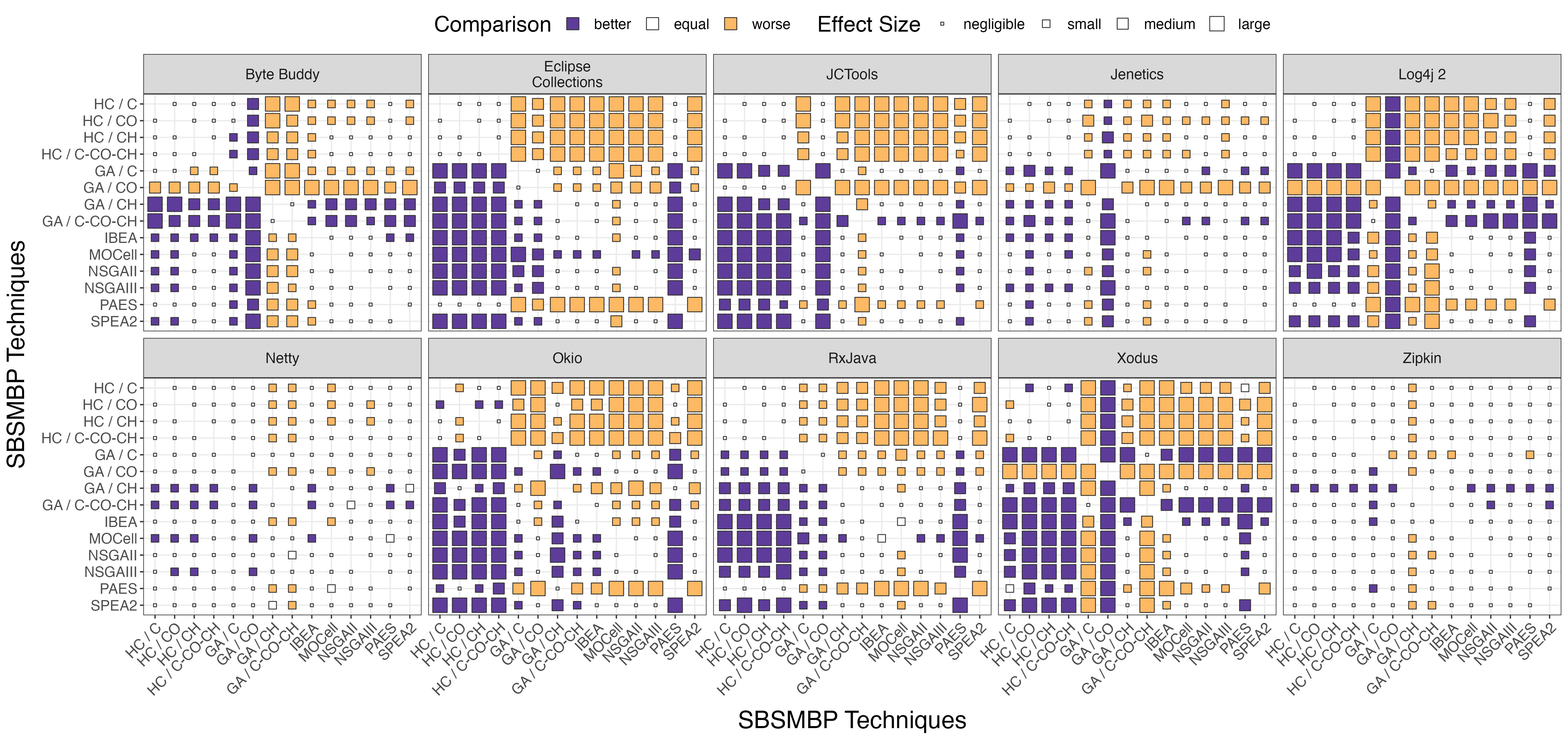
Figure 4: Per project APFD-P effectiveness compared pair-wise for the SBSMBP techniques all the versions and repetitions

Per Project

Table II shows the median APFD-P per project, and Fig. 4 depicts the pair-wise statistical test results. We observe that the effectiveness depends on the project the SMBP technique is applied to. E.g., for GA C-CO-CH, APFD-P ranges from $0.54$ (for Netty) to $0.71$ (for Xodus).

We mostly notice a similar pattern to the overall results, i.e., HC and GA CO perform the worst. The only exception is Okio where GA CO performs well (NSGAII performs even better on median, while the other MOEAs except PAES are also effective). The reason for this is that Okio is the project with the most disjoint coverage sets among the benchmarks and, consequently, a SBSMBP technique with only the CO objective can perform well. Moreover, we observe that for Netty and Zipkin, the SA choice largely does not matter.

The most effective strategies for each project are: (1) GAC-CO-CHfor six, i.e., Byte Buddy, JCTools, Jenetics, Log4j 2, Netty, and Xodus; (2) GACHfor two, i.e., Byte Buddy and Zipkin; (3) MOCellfor two, i.e., Eclipse Collections and RxJava; and (4) NSGAIIand GA CO for one, i.e., Okio.

The reasons why a SA is more effective depends on the characteristics of the studied projects and the problem definition. As we are evaluating the SAs on real-world projects, it is impossible to say which characteristics are responsible for the observed differences. To provide such reasons, we would need to run a controlled experiment where we identify certain project characteristics, create projects and benchmark suites with these, and investigate their impact. Such a study is out-of-scope of this paper.

5.1.2 RQ1b: Comparison to Greedy Techniques

Table III: APFD-P effectiveness for the greedy baselines, four Greedy techniques, and three best SBSMBP techniques from RQ1a; overall and per projects across all the versions and repetitions. The values are the median $\pm$ the MAD.

SMBP Algorithm

Objectives

Overall

Projects

Byte Buddy

Eclipse Collections

JCTools

Jenetics

Log4j 2

Netty

Okio

RxJava

Xodus

Zipkin

Total

–

$0.602816$$\pm$$0.13293288$

$0.4896725$$\pm$$0.25424885$

$0.601873$$\pm$$0.03344301$

$0.6331815$$\pm$$0.12628861$

$0.650411$$\pm$$0.09931789$

$0.648952$$\pm$$0.07221374$

$0.586336$$\pm$$0.09473221$

$0.7045125$$\pm$$0.12551173$

$0.575914$$\pm$$0.10174120$

$0.693962$$\pm$$0.03612577$

$0.447917$$\pm$$0.13534359$

Additional

–

$0.517338$$\pm$$0.16609864$

$0.38419$$\pm$$0.16331061$

$0.603052$$\pm$$0.02898780$

$0.50157$$\pm$$0.04650471$

$0.44029$$\pm$$0.25686638$

$0.502365$$\pm$$0.06530779$

$0.50929$$\pm$$0.05222310$

$0.7402135$$\pm$$0.12734051$

$0.448204$$\pm$$0.13964016$

$0.6106185$$\pm$$0.11977036$

$0.581731$$\pm$$0.19562017$

Greedy

C

$0.602667$$\pm$$0.13289285$

$0.4896725$$\pm$$0.25424885$

$0.598217$$\pm$$0.03606721$

$0.6358535$$\pm$$0.13016413$

$0.650411$$\pm$$0.09931789$

$0.648808$$\pm$$0.06976523$

$0.587018$$\pm$$0.09371070$

$0.7092965$$\pm$$0.12336047$

$0.5747775$$\pm$$0.09944836$

$0.693962$$\pm$$0.03612577$

$0.447917$$\pm$$0.13534359$

CO

$0.44399$$\pm$$0.16841743$

$0.3974495$$\pm$$0.15310365$

$0.587024$$\pm$$0.03910951$

$0.3871065$$\pm$$0.08675286$

$0.376569$$\pm$$0.15896882$

$0.3931485$$\pm$$0.07663930$

$0.424557$$\pm$$0.20268476$

$0.7971935$$\pm$$0.14006938$

$0.413014$$\pm$$0.14220284$

$0.3793575$$\pm$$0.05900081$

$0.555861$$\pm$$0.13533321$

CH

$0.648876$$\pm$$0.14731558$

$0.6727265$$\pm$$0.12932053$

$0.672696$$\pm$$0.04989246$

$0.5126545$$\pm$$0.08583216$

$0.621625$$\pm$$0.31684052$

$0.651328$$\pm$$0.06522773$

$0.484977$$\pm$$0.24299666$

$0.680838$$\pm$$0.17453390$

$0.636202$$\pm$$0.14441043$

$0.582346$$\pm$$0.15888802$

$0.631482$$\pm$$0.15675530$

C-CO-CH

$0.606596$$\pm$$0.14209683$

$0.5002305$$\pm$$0.27572654$

$0.642749$$\pm$$0.03352752$

$0.651003$$\pm$$0.10423568$

$0.62029$$\pm$$0.13936514$

$0.6107625$$\pm$$0.09080777$

$0.597419$$\pm$$0.09438825$

$0.718441$$\pm$$0.15066255$

$0.5821585$$\pm$$0.11220984$

$0.718549$$\pm$$0.06115280$

$0.505342$$\pm$$0.17511730$

GA

CH

$0.583442$$\pm$$0.12850584$

$0.675107$$\pm$$0.14200343$

$0.543922$$\pm$$0.02893739$

$0.592886$$\pm$$0.09239267$

$0.573101$$\pm$$0.27769098$

$0.5795235$$\pm$$0.07246801$

$0.5368515$$\pm$$0.08402191$

$0.588629$$\pm$$0.18009068$

$0.552105$$\pm$$0.07316631$

$0.5881945$$\pm$$0.14516359$

$0.5943285$$\pm$$0.13595071$

C-CO-CH

$0.604286$$\pm$$0.12993655$

$0.6846975$$\pm$$0.13134502$

$0.5459325$$\pm$$0.02823834$

$0.6455615$$\pm$$0.07167259$

$0.5947055$$\pm$$0.20779529$

$0.613514$$\pm$$0.08676991$

$0.5384505$$\pm$$0.08808275$

$0.684705$$\pm$$0.13746890$

$0.5599185$$\pm$$0.07642581$

$0.709417$$\pm$$0.04564258$

$0.5503385$$\pm$$0.16169310$

MOCell

C-CO-CH

$0.577691$$\pm$$0.11929741$

$0.5929615$$\pm$$0.12711553$

$0.5604855$$\pm$$0.03490559$

$0.59627275$$\pm$$0.07057435$

$0.567075$$\pm$$0.20257431$

$0.56095$$\pm$$0.05995078$

$0.5298675$$\pm$$0.07241834$

$0.7630205$$\pm$$0.13285171$

$0.5779695$$\pm$$0.07374045$

$0.642716$$\pm$$0.07615857$

$0.51782875$$\pm$$0.17440787$

This section compares the SBSMBP techniques to the two greedy baselines (i.e., Additional and Total) and four Greedy techniques, one for each objective C, CO, and CH and the combination C-CO-CH (see Section 4.3.3). For brevity, we only investigate the three best SBSMBP techniques from RQ1a, i.e., GA C-CO-CH, GA CH, and MOCell. Table III shows the effectiveness results overall and per project.

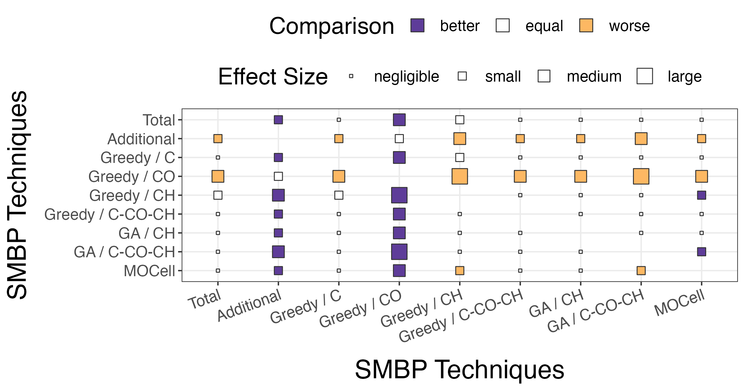
Figure 5: Overall APFD-P effectiveness pairwise comparison among the three best SBSMBP technqiues from RQ1a, the greedy baselines, and the Greedy techniques across all the versions and repetitions

Overall

From Table III’s column “Overall”, we observe that the median APFD-P ranges from $0.44$ to $0.65$, where the two greedy baselines achieve $0.60$ (for Total) and $0.52$ (for Additional). We already found that Total is more effective than Additional for SMBP [56], which might come as a surprise to TCP-savvy readers (e.g., see Luo et al. [63]).

A surprising result is that the SBSMBP techniques are either equal (GA C-CO-CH) or worse (GA CH and MOCell) than Total when considering the median effectiveness. However, our observation aligns with TCP research [63], where the search-based technique is inferior to the greedy baseline (in their case Additional). The statistical tests, depicted in Fig. 5, confirm that the SBSMBP techniques are statistically equal to but never worse than Total and more effective than Additional (with effect sizes small and medium).

The Greedy techniques show a similar pattern as the GA techniques in RQ1a: Greedy CO is the least effective technique overall with $0.44$ APFD-P, Greedy C is equivalent to Total at $0.60$, and both Greedy C-CO-CH with $0.61$ and Greedy CH with $0.65$ are more effective than Total, when considering the median. However, the improvement of the latter two Greedy techniques over Total is not statistically significant (see Fig. 5). Nevertheless, using Greedy CH and achieving a better median effectiveness even though being statistically equivalent is a surprising, yet great result, as it does not require coverage information. RQ2 in Section 5.2 investigates the implications of this on the technique efficiency.

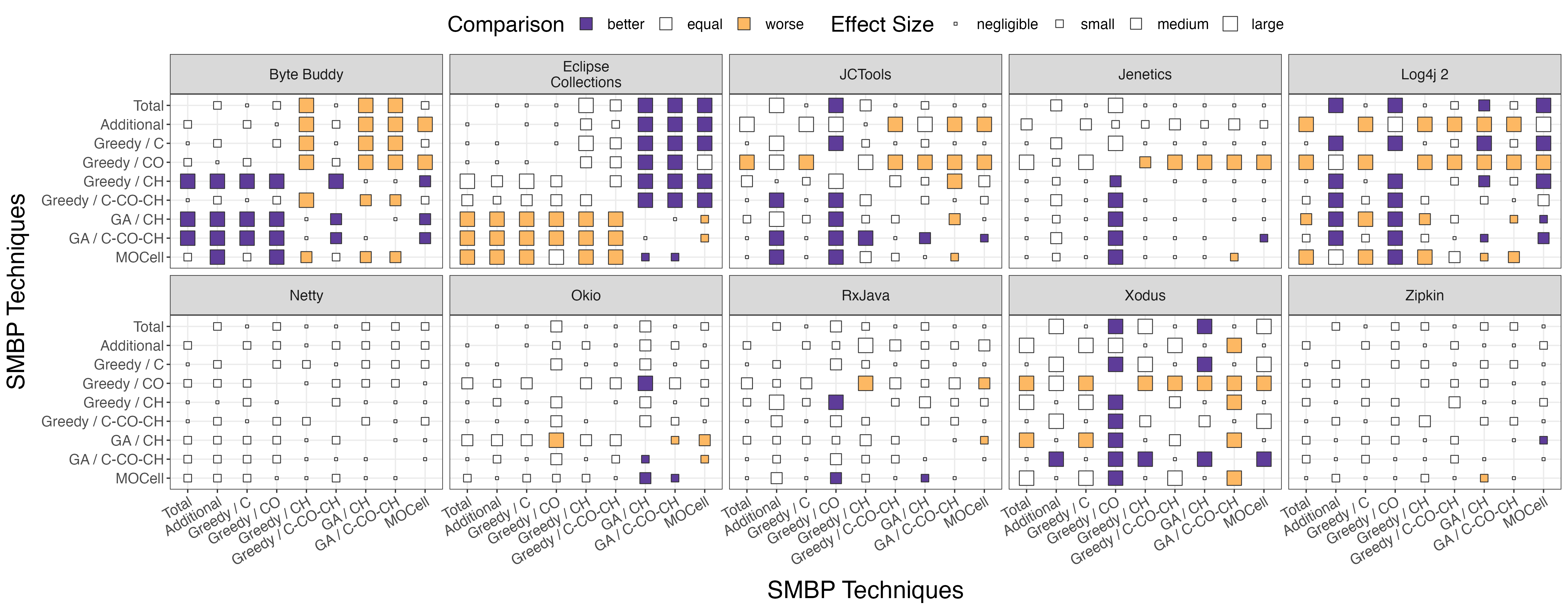
Figure 6: Per project APFD-P effectiveness pairwise comparison among the three best SBSMBP technqiues from RQ1a, the greedy baselines, and the Greedy techniques across all the versions and repetitions

Per Project

While overall the baseline Total is not statistically outperformed by any of the SBSMBP and Greedy techniques, the per-project results offer a nuanced view inTable III and Fig. 6.

The best SBSMBP technique, i.e., GA C-CO-CH is statistically equivalent to Total for eight projects, better for one (Byte Buddy), and worse for one (Eclipse Collections). The other two SBSMBP techniques, i.e., GA CH and MOCell perform worse. GA CH is statistically better than Total for one project (Byte Buddy), worse for three, and equivalent for six, whereas MOCell is never statistically better, worse for two projects, and equivalent for eight. The median differences are in line: (1) GAC-CO-CHis four times better and six times worse than Total; (2) GACHis twice better and eight times worse; and (3) MOCellis three times better, six times worse, and once equal.

The two best Greedy techniques perform favorably compared to Total: (1) GreedyCHis better for one project (Byte Buddy) and equal for nine, while the medians are better for four projects, worse for five, and equal for one; (2) GreedyC-CO-CHis equal for all ten projects, while the medians are better for seven, worse for two, and equal for one.

From a project perspective, the SBSMBP techniques and Greedy CH perform better on Byte Buddy, while just the SBSMBP techniques perform worse on Eclipse Collections. Byte Buddy is the project with the smallest benchmark suite, and Eclipse Collections the one with the largest. However, this suite size trend is not noticeable for the remaining projects. For Jenetics, Netty, Okio, RxJava, and Zipkin, it largely does not matter which technique one chooses as long as it is not Greedy CO and GA CH. For JCTools, Log4j 2, and Xodus any technique except Additional, Greedy CO, GA CH, and MOCell is equally effective.

The most effective strategies according to the median for each project are: (1) GreedyCHfor four, i.e., Eclipse Collections, Log4j 2, RxJava, and Zipkin; (2) GreedyC-CO-CHfor three, i.e., JCTools, Netty, and Xodus; (3) Totalfor two, i.e., Jenetics and Log4j 2; (4) GAC-CO-CHfor two, i.e., Byte Buddy and JCTools; and (5) GACHfor one, i.e., Byte Buddy.

5.1.3 RQ1c: Impact of Change-Awareness

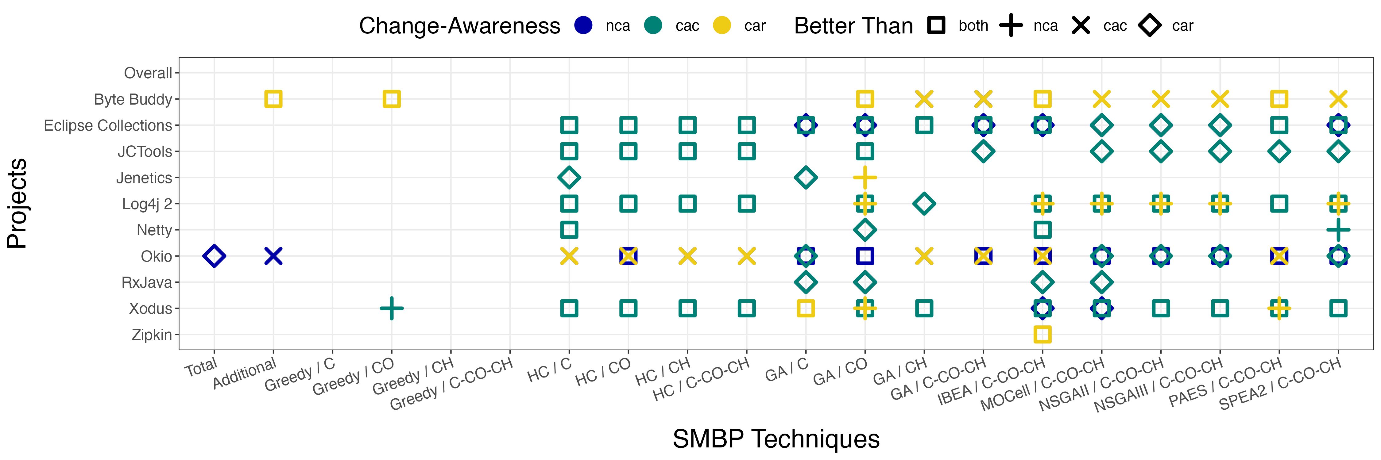
Figure 7: Per project change-awareness pair-wise comparison for each SMBP technique and project across all the versions and repetitions

This section studies if the SMBP techniques from RQ1a and RQ1b perform differently when incorporating change-awareness. Specifically, we compare nca with the two change-aware approaches: cac and car (see Section 4.3.4). Figure 7 depicts the results of the pair-wise statistical tests displayed per project and SMBP technique. For each project and technique, the figure shows which change-awareness approaches are statistically better than which other approaches.

Overall

Contrary to intuition, i.e., a change-aware approach performs better, change-awareness does not improve SMBP effectiveness (see the top row of Fig. 7). To keep the SMBP techniques simple, i.e., not having to manage code change information, this result suggests that nca is the best choice overall.

Per Project

From the overall results, we observe differences among the change-aware approaches, although with no best approach across SMBP techniques and projects. Specifically, greedy techniques are less sensitive to change-awareness, i.e., change-awareness has hardly an impact on effectiveness. Whereas the SBSMBP techniques are considerably impacted by the change-awareness choice, each technique is not equally affected by the same approach. We notice that change-awareness is connected to the project that the SMBP is applied to, e.g., using cac for Byte Buddy is most effective, car for JCTools, and nca for (most SMBP techniques for) Okio. This shows that there often is a benefit for practitioners choosing the “right” change-awareness approach depending on the project and SMBP technique.

5.2 RQ2: Efficiency

While the previous section investigated the effectiveness of the SBSMBP techniques and Greedy techniques, a holistic evaluation requires an efficiency evaluation to understand whether using a technique is feasible in practice. This section compares the greedy heuristics Additional and Total, Greedy techniques, and SBSMBP techniques with respect to the overhead they impose on the overall benchmark suite execution time. Table IV shows the median and MAD efficiency overheads overall and per project. Overheads below $1$% are depicted as “$<1$”. We refrain from reporting statistical tests because they would arguably neither add valuable insights nor change the conclusions.

Table IV: Runtime overhead (prioritization and analysis time) for all the projects and overall for the SMBP techniques

SMBP Algorithm

Objectives

Time

Overall

Projects

Byte Buddy

Eclipse Collections

JCTools

Jenetics

Log4j 2

Netty

Okio

RxJava

Xodus

Zipkin

Total

–

Prioritization

<$1$%$\pm$<$1$

<$1$%$\pm$<$1$

<$1$%$\pm$<$1$

<$1$%$\pm$<$1$

<$1$%$\pm$<$1$

<$1$%$\pm$<$1$

<$1$%$\pm$<$1$

<$1$%$\pm$<$1$

<$1$%$\pm$<$1$

<$1$%$\pm$<$1$

<$1$%$\pm$<$1$

Analysis

$17$%$\pm$<$1$

$13$%$\pm$<$1$

$104$%$\pm$<$1$

$19$%$\pm$<$1$

$8$%$\pm$<$1$

$22$%$\pm$<$1$

$49$%$\pm$<$1$

$14$%$\pm$<$1$

$23$%$\pm$<$1$

$16$%$\pm$<$1$

$20$%$\pm$<$1$

Additional

–

Prioritization

<$1$%$\pm$<$1$

<$1$%$\pm$<$1$

<$1$%$\pm$<$1$

<$1$%$\pm$<$1$

<$1$%$\pm$<$1$

<$1$%$\pm$<$1$

$1$%$\pm$$1$

<$1$%$\pm$<$1$

<$1$%$\pm$<$1$

<$1$%$\pm$<$1$

<$1$%$\pm$<$1$

Analysis

$17$%$\pm$<$1$

$13$%$\pm$<$1$

$105$%$\pm$<$1$

$19$%$\pm$<$1$

$8$%$\pm$<$1$

$22$%$\pm$<$1$

$50$%$\pm$$1$

$14$%$\pm$<$1$

$23$%$\pm$<$1$

$16$%$\pm$<$1$

$20$%$\pm$<$1$

Greedy

C

Prioritization

<$1$%$\pm$<$1$

<$1$%$\pm$<$1$

<$1$%$\pm$<$1$

<$1$%$\pm$<$1$

<$1$%$\pm$<$1$

<$1$%$\pm$<$1$

<$1$%$\pm$<$1$

<$1$%$\pm$<$1$

<$1$%$\pm$<$1$

<$1$%$\pm$<$1$

<$1$%$\pm$<$1$

Analysis

$17$%$\pm$<$1$

$13$%$\pm$<$1$

$104$%$\pm$<$1$

$19$%$\pm$<$1$

$8$%$\pm$<$1$

$22$%$\pm$<$1$

$49$%$\pm$<$1$

$14$%$\pm$<$1$

$23$%$\pm$<$1$

$16$%$\pm$<$1$

$20$%$\pm$<$1$

CO

Prioritization

<$1$%$\pm$<$1$

<$1$%$\pm$<$1$

<$1$%$\pm$<$1$

<$1$%$\pm$<$1$

<$1$%$\pm$<$1$

<$1$%$\pm$<$1$

<$1$%$\pm$<$1$

<$1$%$\pm$<$1$

<$1$%$\pm$<$1$

<$1$%$\pm$<$1$

<$1$%$\pm$<$1$

Analysis

$17$%$\pm$<$1$

$13$%$\pm$<$1$

$104$%$\pm$<$1$

$19$%$\pm$<$1$

$8$%$\pm$<$1$

$22$%$\pm$<$1$

$49$%$\pm$<$1$

$14$%$\pm$<$1$

$23$%$\pm$<$1$

$16$%$\pm$<$1$

$20$%$\pm$<$1$

CH

Prioritization

<$1$%$\pm$<$1$

<$1$%$\pm$<$1$

<$1$%$\pm$<$1$

<$1$%$\pm$<$1$

<$1$%$\pm$<$1$

<$1$%$\pm$<$1$

<$1$%$\pm$<$1$

<$1$%$\pm$<$1$

<$1$%$\pm$<$1$

<$1$%$\pm$<$1$

<$1$%$\pm$<$1$

Analysis

<$1$%$\pm$<$1$

<$1$%$\pm$<$1$

<$1$%$\pm$<$1$

<$1$%$\pm$<$1$

<$1$%$\pm$<$1$

<$1$%$\pm$<$1$

<$1$%$\pm$<$1$

<$1$%$\pm$<$1$

<$1$%$\pm$<$1$

<$1$%$\pm$<$1$

<$1$%$\pm$<$1$

C-CO-CH

Prioritization

<$1$%$\pm$<$1$

<$1$%$\pm$<$1$

<$1$%$\pm$<$1$

<$1$%$\pm$<$1$

<$1$%$\pm$<$1$

<$1$%$\pm$<$1$

<$1$%$\pm$<$1$

<$1$%$\pm$<$1$

<$1$%$\pm$<$1$

<$1$%$\pm$<$1$

<$1$%$\pm$<$1$

Analysis

$17$%$\pm$<$1$

$13$%$\pm$<$1$

$104$%$\pm$<$1$

$19$%$\pm$<$1$

$8$%$\pm$<$1$

$22$%$\pm$<$1$

$49$%$\pm$<$1$

$14$%$\pm$<$1$

$23$%$\pm$<$1$

$16$%$\pm$<$1$

$20$%$\pm$<$1$

HC

C

Prioritization

<$1$%$\pm$<$1$

<$1$%$\pm$<$1$

<$1$%$\pm$<$1$

<$1$%$\pm$<$1$

<$1$%$\pm$<$1$

<$1$%$\pm$<$1$

<$1$%$\pm$<$1$

<$1$%$\pm$<$1$

<$1$%$\pm$<$1$

<$1$%$\pm$<$1$

<$1$%$\pm$<$1$

Analysis

$17$%$\pm$<$1$

$13$%$\pm$<$1$

$104$%$\pm$<$1$

$19$%$\pm$<$1$

$8$%$\pm$<$1$

$22$%$\pm$<$1$

$49$%$\pm$<$1$

$14$%$\pm$<$1$

$23$%$\pm$<$1$

$16$%$\pm$<$1$

$20$%$\pm$<$1$

CO

Prioritization

<$1$%$\pm$<$1$

<$1$%$\pm$<$1$

<$1$%$\pm$<$1$

<$1$%$\pm$<$1$

<$1$%$\pm$<$1$

<$1$%$\pm$<$1$

<$1$%$\pm$<$1$

<$1$%$\pm$<$1$

<$1$%$\pm$<$1$

<$1$%$\pm$<$1$

<$1$%$\pm$<$1$

Analysis

$17$%$\pm$<$1$

$13$%$\pm$<$1$

$104$%$\pm$<$1$

$19$%$\pm$<$1$

$8$%$\pm$<$1$

$22$%$\pm$<$1$

$49$%$\pm$<$1$

$14$%$\pm$<$1$

$23$%$\pm$<$1$

$16$%$\pm$<$1$

$20$%$\pm$<$1$

CH

Prioritization

<$1$%$\pm$<$1$

<$1$%$\pm$<$1$

<$1$%$\pm$<$1$

<$1$%$\pm$<$1$

<$1$%$\pm$<$1$

<$1$%$\pm$<$1$

<$1$%$\pm$<$1$

<$1$%$\pm$<$1$

<$1$%$\pm$<$1$

<$1$%$\pm$<$1$

<$1$%$\pm$<$1$

Analysis

<$1$%$\pm$<$1$

<$1$%$\pm$<$1$

<$1$%$\pm$<$1$

<$1$%$\pm$<$1$

<$1$%$\pm$<$1$

<$1$%$\pm$<$1$

<$1$%$\pm$<$1$

<$1$%$\pm$<$1$

<$1$%$\pm$<$1$

<$1$%$\pm$<$1$

<$1$%$\pm$<$1$

C-CO-CH

Prioritization

<$1$%$\pm$<$1$

<$1$%$\pm$<$1$

<$1$%$\pm$<$1$

<$1$%$\pm$<$1$

<$1$%$\pm$<$1$

<$1$%$\pm$<$1$

<$1$%$\pm$<$1$

<$1$%$\pm$<$1$

<$1$%$\pm$<$1$

<$1$%$\pm$<$1$

<$1$%$\pm$<$1$

Analysis

$17$%$\pm$<$1$

$13$%$\pm$<$1$

$104$%$\pm$<$1$

$19$%$\pm$<$1$

$8$%$\pm$<$1$

$22$%$\pm$<$1$

$49$%$\pm$<$1$

$14$%$\pm$<$1$

$23$%$\pm$<$1$

$16$%$\pm$<$1$

$20$%$\pm$<$1$

GA

C

Prioritization

$1$%$\pm$$1$

$2$%$\pm$$1$

<$1$%$\pm$<$1$

<$1$%$\pm$<$1$

$1$%$\pm$<$1$

<$1$%$\pm$<$1$

<$1$%$\pm$<$1$

<$1$%$\pm$<$1$

<$1$%$\pm$<$1$

<$1$%$\pm$<$1$

$1$%$\pm$<$1$

Analysis

$18$%$\pm$$1$

$15$%$\pm$$1$

$104$%$\pm$<$1$

$19$%$\pm$<$1$

$9$%$\pm$<$1$

$23$%$\pm$<$1$

$49$%$\pm$<$1$

$14$%$\pm$<$1$

$23$%$\pm$<$1$

$16$%$\pm$<$1$

$22$%$\pm$<$1$

CO

Prioritization

$1$%$\pm$$1$

$2$%$\pm$$1$

<$1$%$\pm$<$1$

<$1$%$\pm$<$1$

$1$%$\pm$<$1$

<$1$%$\pm$<$1$

<$1$%$\pm$<$1$

<$1$%$\pm$<$1$

<$1$%$\pm$<$1$

<$1$%$\pm$<$1$

$1$%$\pm$<$1$

Analysis

$19$%$\pm$$1$

$15$%$\pm$$1$

$104$%$\pm$<$1$

$19$%$\pm$<$1$

$9$%$\pm$<$1$

$23$%$\pm$<$1$

$49$%$\pm$<$1$

$14$%$\pm$<$1$

$23$%$\pm$<$1$

$16$%$\pm$<$1$

$22$%$\pm$<$1$

CH

Prioritization

$1$%$\pm$$1$

$2$%$\pm$$1$

<$1$%$\pm$<$1$

<$1$%$\pm$<$1$

$1$%$\pm$<$1$

<$1$%$\pm$<$1$

<$1$%$\pm$<$1$

<$1$%$\pm$<$1$

<$1$%$\pm$<$1$

<$1$%$\pm$<$1$

$1$%$\pm$<$1$

Analysis

$1$%$\pm$$1$

$2$%$\pm$$1$

<$1$%$\pm$<$1$

<$1$%$\pm$<$1$

$1$%$\pm$<$1$

<$1$%$\pm$<$1$

<$1$%$\pm$<$1$

<$1$%$\pm$<$1$

<$1$%$\pm$<$1$

<$1$%$\pm$<$1$

$1$%$\pm$<$1$

C-CO-CH

Prioritization

$1$%$\pm$$1$

$2$%$\pm$$1$

<$1$%$\pm$<$1$

$1$%$\pm$<$1$

$2$%$\pm$<$1$

<$1$%$\pm$<$1$

<$1$%$\pm$<$1$

<$1$%$\pm$<$1$

<$1$%$\pm$<$1$

<$1$%$\pm$<$1$

$1$%$\pm$<$1$

Analysis

$19$%$\pm$$1$

$15$%$\pm$$1$

$104$%$\pm$<$1$

$20$%$\pm$<$1$

$9$%$\pm$<$1$

$23$%$\pm$<$1$

$49$%$\pm$<$1$

$14$%$\pm$<$1$

$23$%$\pm$<$1$

$16$%$\pm$<$1$

$23$%$\pm$<$1$

IBEA

C-CO-CH

Prioritization

$1$%$\pm$$2$

$5$%$\pm$$2$

<$1$%$\pm$<$1$

$1$%$\pm$<$1$

$3$%$\pm$<$1$

$1$%$\pm$<$1$

<$1$%$\pm$<$1$

$1$%$\pm$<$1$

<$1$%$\pm$<$1$

$1$%$\pm$<$1$

$3$%$\pm$$1$

Analysis

$20$%$\pm$$2$

$18$%$\pm$$2$

$104$%$\pm$<$1$

$20$%$\pm$<$1$

$11$%$\pm$<$1$

$23$%$\pm$<$1$

$49$%$\pm$<$1$

$15$%$\pm$<$1$

$23$%$\pm$<$1$

$17$%$\pm$<$1$

$25$%$\pm$$1$

MOCell

C-CO-CH

Prioritization

<$1$%$\pm$<$1$

$3$%$\pm$$1$

<$1$%$\pm$<$1$

<$1$%$\pm$<$1$

$1$%$\pm$<$1$

<$1$%$\pm$<$1$

<$1$%$\pm$<$1$

<$1$%$\pm$<$1$

<$1$%$\pm$<$1$

<$1$%$\pm$<$1$

$1$%$\pm$<$1$

Analysis

$18$%$\pm$<$1$

$15$%$\pm$$1$

$105$%$\pm$<$1$

$19$%$\pm$<$1$

$9$%$\pm$<$1$

$22$%$\pm$<$1$

$49$%$\pm$<$1$

$14$%$\pm$<$1$

$23$%$\pm$<$1$

$16$%$\pm$<$1$

$23$%$\pm$<$1$

NSGAII

C-CO-CH

Prioritization

$1$%$\pm$$1$

$2$%$\pm$$1$

<$1$%$\pm$<$1$

<$1$%$\pm$<$1$

$1$%$\pm$<$1$

<$1$%$\pm$<$1$

<$1$%$\pm$<$1$

<$1$%$\pm$<$1$

<$1$%$\pm$<$1$

<$1$%$\pm$<$1$

$1$%$\pm$<$1$

Analysis

$19$%$\pm$$1$

$15$%$\pm$$1$

$104$%$\pm$<$1$

$20$%$\pm$<$1$

$9$%$\pm$<$1$

$23$%$\pm$<$1$

$49$%$\pm$<$1$

$14$%$\pm$<$1$

$23$%$\pm$<$1$

$16$%$\pm$<$1$

$22$%$\pm$<$1$

NSGAIII

C-CO-CH

Prioritization

<$1$%$\pm$<$1$

<$1$%$\pm$<$1$

<$1$%$\pm$<$1$

<$1$%$\pm$<$1$

<$1$%$\pm$<$1$

<$1$%$\pm$<$1$

<$1$%$\pm$<$1$

<$1$%$\pm$<$1$

<$1$%$\pm$<$1$

<$1$%$\pm$<$1$

<$1$%$\pm$<$1$

Analysis

$17$%$\pm$<$1$

$13$%$\pm$<$1$

$104$%$\pm$<$1$

$19$%$\pm$<$1$

$8$%$\pm$<$1$

$22$%$\pm$<$1$

$49$%$\pm$<$1$

$14$%$\pm$<$1$

$23$%$\pm$<$1$

$16$%$\pm$<$1$

$21$%$\pm$<$1$

PAES

C-CO-CH

Prioritization

<$1$%$\pm$<$1$

<$1$%$\pm$<$1$

<$1$%$\pm$<$1$

<$1$%$\pm$<$1$

<$1$%$\pm$<$1$

<$1$%$\pm$<$1$

<$1$%$\pm$<$1$

<$1$%$\pm$<$1$

<$1$%$\pm$<$1$

<$1$%$\pm$<$1$

<$1$%$\pm$<$1$

Analysis

$17$%$\pm$<$1$

$13$%$\pm$<$1$

$104$%$\pm$<$1$

$19$%$\pm$<$1$

$8$%$\pm$<$1$

$22$%$\pm$<$1$

$49$%$\pm$<$1$

$14$%$\pm$<$1$

$23$%$\pm$<$1$

$16$%$\pm$<$1$

$21$%$\pm$<$1$

SPEA2

C-CO-CH

Prioritization

$2$%$\pm$$2$

$9$%$\pm$$3$

<$1$%$\pm$<$1$

$1$%$\pm$<$1$

$5$%$\pm$$1$

$1$%$\pm$<$1$

<$1$%$\pm$<$1$

$1$%$\pm$<$1$

<$1$%$\pm$<$1$

$1$%$\pm$<$1$

$3$%$\pm$$1$

Analysis

$22$%$\pm$$2$

$22$%$\pm$$3$

$105$%$\pm$<$1$

$20$%$\pm$<$1$

$13$%$\pm$$1$

$23$%$\pm$<$1$

$49$%$\pm$<$1$

$15$%$\pm$<$1$

$23$%$\pm$<$1$

$17$%$\pm$<$1$

$26$%$\pm$$1$

Overall

Both baselines add less than $1$% for running the algorithm, i.e., prioritization time, and combined with the coverage extraction time have a total runtime overhead, i.e., analysis time, of $17$%. This shows that the analysis time is dominated by the coverage extraction and the SMBP algorithm plays only a minor role. These numbers are from the data set of our previous work [56]. The same applies to (most of) the Greedy techniques.

The single-objective SBSMBP techniques (i.e., HC and GA) have around $1$% prioritization time. This brings the analysis time to between $17$% and $19$%, similar to the greedy baselines. Greedy CH, HC CH, and GA CH, however, have a similar analysis and prioritization time. This is because the CH objective does not rely on coverage extraction, which takes the majority of the analysis time for coverage-based techniques. In particular, Greedy CH becomes (even more) appealing, as it is not only the most effective technique (or at least equal to Total) but also the most efficient one.

Regarding the multi-objective SBSMBP technique, we observe that the overall overheads do not change for the majority of the MOEAs, i.e., MOCell (the most effective MOEA from RQ1, see Section 5.1), NSGAII, NSGAIII, and PAES. Only IBEA and SPEA2 encounter a slightly larger prioritization time, which increases the analysis time to $19$% and $21$%, respectively. Given the large suite runtimes (see Table I), this slight increase over the greedy techniques can be considered acceptable.

Per Project

The results per project show a diverse situation for the SMBP techniques that rely on coverage objectives: the analysis times range from between $8$% and $13$% for Jenetics to between $104$% and $105$% for Eclipse Collections. For eight of the projects, the analysis time is $23$% or below. For Eclipse Collections and Netty, where the overhead is $105$% and $49$% respectively, applying SMBP is not worthwhile.

These project-dependent overheads suggest that the techniques with non-coverage-based objectives are critical to be universally applicable across projects, especially when run as part of CI. Hence, the overhead results for the CH techniques are especially promising: all CH techniques have an analysis time overhead of $2$% or less across all the projects. When considering the most effective technique Greedy CH, the overhead even drops below $1$% for all the projects. Consequently, the analysis time of the techniques with non-coverage-based objectives is solely dependent on the prioritization time (i.e., the time taken to run the SMBP algorithm), which will likely always be considerably smaller than the extensive benchmark suite runtimes; therefore, these SMBP techniques are generally beneficial being applied to microbenchmarks.

6 Discussion

The results show that the best SBSMBP technique (GA C-CO-CH) is only competitive with the best greedy baseline (Total). When using a simple Greedy technique that only considers the historical performance change size (CH), one can retrieve more effective SMBP rankings with significantly lower overhead than when relying on coverage objectives (C and CO), which is the case for both the greedy baselines and the SBSMBP techniques. This section discusses our empirical results from several different perspectives.

The Underperforming Search-Based Techniques

The success of the Greedy CH technique in terms of effectiveness begs the question, why are the SBSMBP techniques underperforming in our study? We see the following two reasons.

First, coverage is not “good enough” as objectives for SMBP. This becomes evident from this and our previous study [56]. Furthermore, Chen et al. [11] observed that in the context of benchmark selection, functional bug prediction metrics are more important than code-level performance metrics. This suggests that future SMBP techniques should explore dedicated metrics related to size, diffusion, or history as well as specific code-level performance metrics, such as loops or synchronization (similar to Laaber et al. [55]). However, given the high coverage extraction overhead, non-code metrics should be more favoured than code ones.

Second, optimal hyperparameters of the SAs could improve SBSMBP effectiveness. However, we explored the effectiveness of the SAs with more generations and investigated the convergence of the objectives and found that the objectives converge quickly. This suggests that the search space is relatively trivial (for the given objectives) and SAs do not offer an advantage over simple greedy techniques, which our results empirically show. Moreover, the search objectives we employed, in particular the coverage-based objectives, are not effective in finding bigger performance changes sooner, and other objectives should be explored in the future (such as the ones mentioned above).

Is it Worth Applying SMBP? While coverage-based SMBP is effective, there is still a considerable overhead. This overhead is mostly due to the time required to extract coverage information [56] and only a small fraction is attributed to the prioritization algorithm (see Section 5.2). While this time is arguably lower than for unit testing because benchmarks are repeatedly executed and run much longer [54], whether it is worth employing coverage-based SMBP highly depends on the individual benchmark suite and the project’s performance testing objectives. If it is critical to detect performance changes as fast as possible, e.g., the release of a new software version would be otherwise halted, running SMBP can drastically reduce the time to detect these. However, for projects with extensive overheads, such as Eclipse Collections and Netty in our study, coverage-based SMBP is not worthwhile. A better alternative to coverage-based techniques are SMBP techniques that solely rely on the CH objective, which is (sometimes) more effective and substantially more efficient. This suggests that non-coverage-based SMBP techniques are highly suggested to be employed.

Is it Practical to Apply SMBP? Beyond the temporal cost of applying a SMBP technique, there is a cost of extracting and maintaining the information required as input. On the one hand, the techniques require storing historical information about benchmark executions, especially their changes between previous versions, for computing the CH objective. On the other hand, there is neither a need to store historical coverage information nor compute the source code difference on every new commit, as the results of RQ1c show that nca, the non-change-aware approach, perform equal to the change-aware approaches (i.e., cac and car) overall. This is probably best done as part of the CI pipeline because it provides the necessary infrastructure to run benchmarks, store the information about the build (i.e., performance change history), and has the code changes readily available.

Relying on Measured Performance Changes

Research on functional TCP often uses datasets with seeded, artificial faults (mutations) to evaluate TCP effectiveness (e.g., [64, 22]). Conversely, performance regression testing research mostly relies on measured performance changes between adjacent versions [67, 56]. This is due to performance mutation testing having only recently received attention [20, 42] and large datasets, such as Defects4J [44], not existing. Because of the enormous experiment runtimes required for rigorously executing benchmarks (this study’s dataset took $89$ days to create), performing performance mutation testing, where for each mutant the whole benchmark suite has to be executed, becomes unrealistic. However, this does not invalidate the findings of this study or any other experimental performance regression study relying on measured performance changes as long as the measurements have been conducted rigorously.

Moreover, measuring performance captures changes stemming from “outside” the software under test (SUT), e.g., its dependencies or runtime environment. While it is harder for techniques to also detect these changes, it makes the evaluation more realistic, as the SUT’s developers should be aware of any observable performance changes, irrespective of their origin, to take adequate action.

What is an Important Performance Change? Following previous research on SMBP [67, 56], this paper also defines the importance of a benchmark as the performance change size it detects. A benchmark that detects a large performance change is considered more important than a benchmark that detects a small one. Accordingly, we conclude whether a technique is more or less effective. It is, however, unclear whether this definition of importance is “accurate.” Alternative formulations of importance could be based on: (1) the impact of the code called by the benchmark on the performance of an application, (2) the project developer’s perception and context-dependent knowledge, or (3) the usage frequency of the code from application programming interface (API) clients. Moreover, developers might consider a performance change, irrespective of its size, as important. All these different definitions of importance would likely change this paper’s results and require a study of its own.

7 Related Work

This section discusses the related work on (1) search-based regression testing and (2) software performance testing.

7.1 Search-Based Regression Testing

Regression testing on unit tests has been a well-established research field for the last $30$ years [81]. The three main techniques in regression testing are test suite minimization, RTS, and TCP. Traditionally, techniques relied on greedy heuristics, such as Additional and Total coverage, to solve the optimization problems of selecting the best subset or prioritizing the most fault-revealing tests [72, 73, 24].

Based on the early success of search techniques in software engineering [36], regression testing techniques were quickly adapted to use search for the optimization. Yoo and Harman [82] formulate RTS as a multi-objective optimization problem and generate Pareto optimal solutions [28]. Li et al. [60] are the first to apply search to TCP by introducing coverage-based objectives based on block, decision, and statement granularity. Our work is inspired by theirs and adapts the objectives for SMBP.

Li et al. [61] take the idea a step forward and introduce multi-objective, search-based TCP with NSGAII and two objectives: coverage and execution time. Islam et al. [41] and Marchetto et al. [65] consider three objectives and apply different weights to these. Epitropakis et al. [27] address the $\mathcal{O}(mn)$ complexity of the fitness function by devising a coverage compaction algorithm and consider historical faults as an objective. Finally, Di Nucci et al. [22] introduce a new search algorithm based on the hypervolume [7]. Our work builds on all these in terms of inspiration for the search objectives and the experimental setup (see Section 4.3) and ports them to the problem of prioritizing microbenchmarks.

7.2 Software Performance Testing

Performance testing with microbenchmarks is a relatively new area of research. To this end, earlier studies investigate unit-level performance testing on OSS Java projects [59, 76], which conclude that it is still a niche technique, especially compared to unit testing. Explanations could be that more effort is required to write microbenchmarks, the extra cost of their execution, and the higher complexity required to assess the results with statistical analyses. Samoaa and Leitner [75] investigate parameterization of benchmarks in detail. Grambow et al. [31, 32] utilize information from application benchmarks to guide microbenchmark execution and assess the ability of microbenchmarks to detect application performance changes, with limited success. He et al. [37] and Laaber et al. [54] take an orthogonal approach to optimizing performance testing: they dynamically stop benchmarks when their results are of a desired statistical quality instead of optimizing the execution order of the benchmark suite. Traini et al. [79] further assess whether dynamically stopping is beneficially for measuring in steady state.

There exist works on performance regression testing, i.e., greedy heuristics [17], genetic algorithms [3, 4], and machine learning [11] have been used to select the optimal benchmarks for a given software version in terms of their ability to find performance changes. These works focus on RTS whereas this paper targets SMBP. In addition, some works exist for performance regression testing of concurrent classes (e.g., [70, 83]). They focus on concurrent software and generate tests for these, whereas this paper optimizes the execution of existing benchmark suites. Finally, Huang et al. [40] proposed a prediction method to assess the need for performance testing of a new software version, which targets the version level compared to ours on the benchmark level.

We consider two works on performance regression testing closely related to ours [67, 56]. For a given software version, Mostafa et al. [67] prioritize test cases with complex performance impact analysis that requires measuring individual components of not only the SUT but also the Java Development Kit (JDK). Their technique focuses on collection-intensive software and is partially only evaluated on unit tests used as performance tests, whereas our technique is generally applicable to any kind of software and is evaluated only on benchmarks. Laaber et al. [56] studied coverage-based, greedy SMBP techniques and found that they are only marginally more effective than a random ordering. We build on their work and use SAs and novel Greedy techniques instead.

8 Conclusions and Future Work

This paper defines SBSMBP and Greedy SMBP techniques relying on three objectives: coverage, coverage overlap among benchmarks, and performance change size obtained from historical data. With an extensive experimental evaluation on $10$ Java projects with JMH suites, we study the effectiveness and efficiency of a total of $18$ new SMBP techniques and compare these to two coverage-based, greedy SMBP baselines. The results reveal that the best SBSMBP technique is competitive with the best greedy baselines but does not improve on its effectiveness. Surprisingly, the Greedy technique relying only on the historical performance change size can be more effective than the best coverage-based greedy baselines and SBSMBP techniques while being significantly more efficient.

This paper provides evidence that SMBP is a difficult problem to solve and more work is required going forward. Hence, we envision future research to (1) assess SMBP on performance mutations and developer-reported performance bugs, (2) investigate novel algorithms (potentially search-based) specifically targeting SMBP, and (3) devise process- and performance-focused, ideally non-coverage-based, objectives that serve as better proxies for performance changes than the ones studied here.

References

- Achimugu et al. [2014] P. Achimugu, A. Selamat, R. Ibrahim, and M. N. Mahrin, “A systematic literature review of software requirements prioritization research,” Information and Software Technology, vol. 56, no. 6, 2014. [Online]. Available: https://doi.org/10.1016/j.infsof.2014.02.001
- Alshahwan et al. [2023] N. Alshahwan, M. Harman, and A. Marginean, “Software testing research challenges: An industrial perspective,” in Proceedings of the 16th IEEE International Conference on Software Testing, Verification and Validation, ser. ICST 2023. IEEE, 2023. [Online]. Available: https://doi.org/10.1109/ICST57152.2023.00008
- Alshoaibi et al. [2019] D. Alshoaibi, K. Hannigan, H. Gupta, and M. W. Mkaouer, “PRICE: Detection of performance regression introducing code changes using static and dynamic metrics,” in Proceedings of the 11th International Symposium on Search Based Software Engineering, ser. SSBSE 2019. Springer Nature, 2019. [Online]. Available: https://doi.org/10.1007/978-3-030-27455-9_6
- Alshoaibi et al. [2022] D. Alshoaibi, M. W. Mkaouer, A. Ouni, A. Wahaishi, T. Desell, and M. Soui, “Search-based detection of code changes introducing performance regression,” Swarm and Evolutionary Computation, vol. 73, 2022. [Online]. Available: https://doi.org/10.1016/j.swevo.2022.101101
- Arcuri [2019] A. Arcuri, “RESTful API automated test case generation with EvoMaster,” ACM Transactions on Software Engineering and Methodology, vol. 28, no. 1, 2019. [Online]. Available: https://doi.org/10.1145/3293455
- Arcuri and Briand [2011] A. Arcuri and L. Briand, “A practical guide for using statistical tests to assess randomized algorithms in software engineering,” in Proceedings of the 33rd International Conference on Software Engineering, ser. ICSE 2011. ACM, 2011. [Online]. Available: https://doi.org/10.1145/1985793.1985795
- Auger et al. [2009] A. Auger, J. Bader, D. Brockhoff, and E. Zitzler, “Theory of the hypervolume indicator: Optimal µ-distributions and the choice of the reference point,” in Proceedings of the 10th ACM SIGEVO Workshop on Foundations of Genetic Algorithms, ser. FOGA 2009. ACM, 2009. [Online]. Available: https://doi.org/10.1145/1527125.1527138
- Benjamini and Yekutieli [2001] Y. Benjamini and D. Yekutieli, “The control of the false discovery rate in multiple testing under dependency,” The Annals of Statistics, vol. 29, no. 4, 2001. [Online]. Available: https://doi.org/10.1214/aos/1013699998
- Branke et al. [2004] J. Branke, K. Deb, H. Dierolf, and M. Osswald, “Finding knees in multi-objective optimization,” in Proceedings of the 8th International Conference on Parallel Problem Solving from Nature, ser. PPSN 2004. Springer, 2004.
- Chen and Shang [2017] J. Chen and W. Shang, “An exploratory study of performance regression introducing code changes,” in Proceedings of the 33rd IEEE International Conference on Software Maintenance and Evolution, ser. ISCME 2017. IEEE, 2017. [Online]. Available: https://doi.org/10.1109/icsme.2017.13
- Chen et al. [2020] J. Chen, W. Shang, and E. Shihab, “PerfJIT: Test-level just-in-time prediction for performance regression introducing commits,” IEEE Transactions on Software Engineering, 2020. [Online]. Available: https://doi.org/10.1109%2Ftse.2020.3023955
- Chen et al. [2021] K. Chen, Y. Li, Y. Chen, C. Fan, Z. Hu, and W. Yang, “GLIB: Towards automated test oracle for graphically-rich applications,” in Proceedings of the 29th ACM Joint European Software Engineering Conference and Symposium on the Foundations of Software Engineering, ser. ESEC/FSE 2021. ACM, 2021. [Online]. Available: https://doi.org/10.1145/3468264.3468586
- Daly [2021] D. Daly, “Creating a virtuous cycle in performance testing at MongoDB,” in Proceedings of the 12th ACM/SPEC International Conference on Performance Engineering, ser. ICPE 2021. ACM, 2021. [Online]. Available: https://doi.org/10.1145/3427921.3450234
- Daly et al. [2020] D. Daly, W. Brown, H. Ingo, J. O'Leary, and D. Bradford, “The use of change point detection to identify software performance regressions in a continuous integration system,” in Proceedings of the 11th ACM/SPEC International Conference on Performance Engineering, ser. ICPE 2020. ACM, 2020. [Online]. Available: https://doi.org/10.1145/3358960.3375791
- Damasceno Costa et al. [2019] D. E. Damasceno Costa, C.-P. Bezemer, P. Leitner, and A. Andrzejak, “What’s wrong with my benchmark results? Studying bad practices in JMH benchmarks,” IEEE Transactions on Software Engineering, 2019.
- Davison and Hinkley [1997] A. C. Davison and D. Hinkley, “Bootstrap methods and their application,” Journal of the American Statistical Association, vol. 94, 1997.
- de Oliveira et al. [2017] A. B. de Oliveira, S. Fischmeister, A. Diwan, M. Hauswirth, and P. F. Sweeney, “Perphecy: Performance regression test selection made simple but effective,” in Proceedings of the 10th IEEE International Conference on Software Testing, Verification and Validation, ser. ICST 2017, 2017.
- Deb and Jain [2014] K. Deb and H. Jain, “An evolutionary many-objective optimization algorithm using reference-point-based nondominated sorting approach, part I: Solving problems with box constraints,” IEEE Transactions on Evolutionary Computation, vol. 18, no. 4, 2014. [Online]. Available: https://doi.org/10.1109%2Ftevc.2013.2281535
- Deb et al. [2002] K. Deb, A. Pratap, S. Agarwal, and T. Meyarivan, “A fast and elitist multiobjective genetic algorithm: NSGA-II,” IEEE Transactions on Evolutionary Computation, vol. 6, no. 2, 2002. [Online]. Available: https://doi.org/10.1109%2F4235.996017
- Delgado-Pérez et al. [2020] P. Delgado-Pérez, A. B. Sánchez, S. Segura, and I. Medina-Bulo, “Performance mutation testing,” Software Testing, Verification and Reliability, vol. 31, no. 5, 2020. [Online]. Available: https://doi.org/10.1002/stvr.1728
- Devroey et al. [2023] X. Devroey, A. Gambi, J. P. Galeotti, R. Just, F. M. Kifetew, A. Panichella, and S. Panichella, “JUGE: An infrastructure for benchmarking Java unit test generators,” Software Testing, Verification and Reliability, vol. 33, no. 3, 2023. [Online]. Available: https://doi.org/10.1002/stvr.1838
- Di Nucci et al. [2020] D. Di Nucci, A. Panichella, A. Zaidman, and A. De Lucia, “A test case prioritization genetic algorithm guided by the hypervolume indicator,” IEEE Transactions on Software Engineering, vol. 46, no. 6, 2020. [Online]. Available: https://doi.org/10.1109/tse.2018.2868082
- Dunn [1964] O. J. Dunn, “Multiple comparisons using rank sums,” Technometrics, vol. 6, no. 3, 1964. [Online]. Available: https://doi.org/10.1080/00401706.1964.10490181
- Elbaum et al. [2001] S. Elbaum, A. Malishevsky, and G. Rothermel, “Incorporating varying test costs and fault severities into test case prioritization,” in Proceedings of the 23rd International Conference on Software Engineering, ser. ICSE 2001. IEEE, 2001. [Online]. Available: https://doi.org/10.1109/icse.2001.919106
- Elbaum et al. [2014] S. Elbaum, G. Rothermel, and J. Penix, “Techniques for improving regression testing in continuous integration development environments,” in Proceedings of the 22nd ACM SIGSOFT International Symposium on Foundations of Software Engineering, ser. FSE 2014. ACM, 2014. [Online]. Available: http://doi.acm.org/10.1145/2635868.2635910
- Elsner et al. [2021] D. Elsner, F. Hauer, A. Pretschner, and S. Reimer, “Empirically evaluating readily available information for regression test optimization in continuous integration,” in Proceedings of the 30th ACM SIGSOFT International Symposium on Software Testing and Analysis, ser. ISSTA 2021. ACM, 2021. [Online]. Available: https://doi.org/10.1145/3460319.3464834
- Epitropakis et al. [2015] M. G. Epitropakis, S. Yoo, M. Harman, and E. K. Burke, “Empirical evaluation of pareto efficient multi-objective regression test case prioritisation,” in Proceedings of the 2015 International Symposium on Software Testing and Analysis, ser. ISSTA 2015. ACM, 2015. [Online]. Available: https://doi.org/10.1145/2771783.2771788
- Fonseca and Fleming [1995] C. M. Fonseca and P. J. Fleming, “An overview of evolutionary algorithms in multiobjective optimization,” Evolutionary Computation, vol. 3, no. 1, 1995. [Online]. Available: https://doi.org/10.1162/evco.1995.3.1.1
- Fraser and Zeller [2010] G. Fraser and A. Zeller, “Mutation-driven generation of unit tests and oracles,” in Proceedings of the 19th International Symposium on Software Testing and Analysis, ser. ISSTA 2010. ACM, 2010. [Online]. Available: https://doi.org/10.1145/1831708.1831728
- Georges et al. [2007] A. Georges, D. Buytaert, and L. Eeckhout, “Statistically rigorous Java performance evaluation,” in Proceedings of the 22nd ACM SIGPLAN Conference on Object-Oriented Programming, Systems, and Applications, ser. OOPSLA 2007. ACM, 2007. [Online]. Available: http://doi.acm.org/10.1145/1297027.1297033
- Grambow et al. [2021] M. Grambow, C. Laaber, P. Leitner, and D. Bermbach, “Using application benchmark call graphs to quantify and improve the practical relevance of microbenchmark suites,” PeerJ Computer Science, vol. 7, 2021. [Online]. Available: https://doi.org/10.7717/peerj-cs.548
- Grambow et al. [2022] M. Grambow, D. Kovalev, C. Laaber, P. Leitner, and D. Bermbach, “Using microbenchmark suites to detect application performance changes,” IEEE Transactions on Cloud Computing, 2022.
- Haghighatkhah et al. [2018] A. Haghighatkhah, M. Mäntylä, M. Oivo, and P. Kuvaja, “Test prioritization in continuous integration environments,” The Journal of Systems and Software, vol. 146, 2018. [Online]. Available: https://doi.org/10.1016/j.jss.2018.08.061
- Hao et al. [2014] D. Hao, L. Zhang, L. Zhang, G. Rothermel, and H. Mei, “A unified test case prioritization approach,” ACM Transactions on Software Engineering and Methodology, vol. 24, no. 2, 2014. [Online]. Available: http://doi.acm.org/10.1145/2685614
- Harman [2007] M. Harman, “The current state and future of search based software engineering,” in Future of Software Engineering, ser. FOSE 2007. IEEE, 2007. [Online]. Available: https://doi.org/10.1109/fose.2007.29
- Harman and Jones [2001] M. Harman and B. F. Jones, “Search-based software engineering,” Information and Software Technology, vol. 43, no. 14, 2001. [Online]. Available: https://doi.org/10.1016/S0950-5849(01)00189-6
- He et al. [2019] S. He, G. Manns, J. Saunders, W. Wang, L. Pollock, and M. L. Soffa, “A statistics-based performance testing methodology for cloud applications,” in Proceedings of the 27th ACM Joint European Software Engineering Conference and Symposium on the Foundations of Software Engineering, ser. ESEC/FSE 2019. ACM, 2019. [Online]. Available: http://doi.acm.org/10.1145/3338906.3338912
- Hess and Kromrey [2004] M. R. Hess and J. D. Kromrey, “Robust confidence intervals for effect sizes: A comparative study of cohen’s d and cliff’s delta under non-normality and heterogeneous variances,” Annual Meeting of the American Educational Research Association, 2004.
- Hesterberg [2015] T. C. Hesterberg, “What teachers should know about the bootstrap: Resampling in the undergraduate statistics curriculum,” The American Statistician, vol. 69, no. 4, 2015. [Online]. Available: https://doi.org/10.1080/00031305.2015.1089789
- Huang et al. [2014] P. Huang, X. Ma, D. Shen, and Y. Zhou, “Performance regression testing target prioritization via performance risk analysis,” in Proceedings of the 36th IEEE/ACM International Conference on Software Engineering, ser. ICSE 2014. ACM, 2014. [Online]. Available: http://doi.acm.org/10.1145/2568225.2568232
- Islam et al. [2012] M. M. Islam, A. Marchetto, A. Susi, and G. Scanniello, “A multi-objective technique to prioritize test cases based on latent semantic indexing,” in Proceedings of the 16th European Conference on Software Maintenance and Reengineering, ser. CSMR 2012. IEEE, 2012. [Online]. Available: https://doi.org/10.1109/csmr.2012.13
- Jangali et al. [2022] M. Jangali, Y. Tang, N. Alexandersson, P. Leitner, J. Yang, and W. Shang, “Automated generation and evaluation of JMH microbenchmark suites from unit tests,” IEEE Transactions on Software Engineering, 2022. [Online]. Available: https://doi.org/10.1109/TSE.2022.3188005
- Jiang and Hassan [2015] Z. M. Jiang and A. E. Hassan, “A survey on load testing of large-scale software systems,” IEEE Transactions on Software Engineering, vol. 41, no. 11, 2015. [Online]. Available: https://doi.org/10.1109/tse.2015.2445340
- Just et al. [2014] R. Just, D. Jalali, and M. D. Ernst, “Defects4J: A database of existing faults to enable controlled testing studies for Java programs,” in Proceedings of the 2014 International Symposium on Software Testing and Analysis, ser. ISSTA 2014. ACM, 2014. [Online]. Available: https://doi.org/10.1145/2610384.2628055
- Kalibera and Jones [2012] T. Kalibera and R. Jones, “Quantifying performance changes with effect size confidence intervals,” University of Kent, Technical Report 4–12, 2012. [Online]. Available: http://www.cs.kent.ac.uk/pubs/2012/3233
- Kalibera and Jones [2013] ——, “Rigorous benchmarking in reasonable time,” in Proceedings of the 2013 ACM SIGPLAN International Symposium on Memory Management, ser. ISMM 2013. ACM, 2013. [Online]. Available: http://doi.acm.org/10.1145/2464157.2464160
- Kim et al. [2004] M. Kim, T. Hiroyasu, M. Miki, and S. Watanabe, “SPEA2+: Improving the performance of the strength pareto evolutionary algorithm 2,” in Proceedings of the 8th International Conference on Parallel Problem Solving from Nature, ser. PPSN 2004, vol. 3242. Springer, 2004. [Online]. Available: https://doi.org/10.1007%2F978-3-540-30217-9_75
- Knowles and Corne [1999] J. D. Knowles and D. Corne, “The Pareto aarchived evolution strategy: A new baseline algorithm for Pareto Multiobjective optimisation,” in Proceedings of the Congress on Evolutionary Computation, ser. CEC 1999. IEEE, 1999. [Online]. Available: https://doi.org/10.1109/cec.1999.781913
- Kruskal and Wallis [1952] W. H. Kruskal and W. A. Wallis, “Use of ranks in one-criterion variance analysis,” Journal of the American Statistical Association, vol. 47, no. 260, 1952. [Online]. Available: https://doi.org/10.1080/01621459.1952.10483441
- Laaber [2022] C. Laaber, “chrstphlbr/pa: v0.1.0,” Nov. 2022. [Online]. Available: https://doi.org/10.5281/zenodo.7308066
- Laaber and Leitner [2018] C. Laaber and P. Leitner, “An evaluation of open-source software microbenchmark suites for continuous performance assessment,” in Proceedings of the 15th International Conference on Mining Software Repositories, ser. MSR 2018. ACM, 2018. [Online]. Available: http://doi.acm.org/10.1145/3196398.3196407
- Laaber and Würsten [2024] C. Laaber and S. Würsten, “chrstphlbr/bencher: Release v0.4.0,” Jan. 2024. [Online]. Available: https://doi.org/10.5281/zenodo.10527360
- Laaber et al. [2019] C. Laaber, J. Scheuner, and P. Leitner, “Software microbenchmarking in the cloud. How bad is it really?” Empirical Software Engineering, vol. 24, 2019. [Online]. Available: https://doi.org/10.1007/s10664-019-09681-1
- Laaber et al. [2020] C. Laaber, S. Würsten, H. C. Gall, and P. Leitner, “Dynamically reconfiguring software microbenchmarks: Reducing execution time without sacrificing result quality,” in Proceedings of the 28th ACM Joint European Software Engineering Conference and Symposium on the Foundations of Software Engineering, ser. ESEC/FSE 2020. ACM, 2020. [Online]. Available: https://doi.org/10.1145/3368089.3409683
- Laaber et al. [2021c] C. Laaber, M. Basmaci, and P. Salza, “Predicting unstable software benchmarks using static source code features,” Empirical Software Engineering, vol. 26, no. 6, 2021. [Online]. Available: https://doi.org/10.1007/s10664-021-09996-y
- Laaber et al. [2021a] C. Laaber, H. C. Gall, and P. Leitner, “Applying test case prioritization to software microbenchmarks,” Empirical Software Engineering, vol. 26, no. 6, 2021. [Online]. Available: https://doi.org/10.1007/s10664-021-10037-x
- Laaber et al. [2021b] ——, “Replication package "Applying test case prioritization to software microbenchmarks",” 2021. [Online]. Available: https://doi.org/10.5281/zenodo.5206117
- Laaber et al. [2024] C. Laaber, T. Yue, and S. Ali, “Replication package "Evaluating search-based software microbenchmark prioritization",” 2024. [Online]. Available: https://doi.org/10.5281/zenodo.10527125
- Leitner and Bezemer [2017] P. Leitner and C.-P. Bezemer, “An exploratory study of the state of practice of performance testing in Java-based open source projects,” in Proceedings of the 8th ACM/SPEC on International Conference on Performance Engineering, ser. ICPE 2017. ACM, 2017. [Online]. Available: http://doi.acm.org/10.1145/3030207.3030213
- Li et al. [2007] Z. Li, M. Harman, and R. M. Hierons, “Search algorithms for regression test case prioritization,” IEEE Transactions on Software Engineering, vol. 33, no. 4, 2007. [Online]. Available: https://doi.org/10.1109/TSE.2007.38
- Li et al. [2013] Z. Li, Y. Bian, R. Zhao, and J. Cheng, “A fine-grained parallel multi-objective test case prioritization on GPU,” in Proceedings of the 5th Symposium on Search Based Software Engineering, ser. SSBSE 2013. Springer, 2013. [Online]. Available: https://doi.org/10.1007/978-3-642-39742-4_10
- Liang et al. [2018] J. Liang, S. Elbaum, and G. Rothermel, “Redefining prioritization: Continuous prioritization for continuous integration,” in Proceedings of the 40th IEEE/ACM International Conference on Software Engineering, ser. ICSE 2018. ACM, 2018. [Online]. Available: http://doi.acm.org/10.1145/3180155.3180213
- Luo et al. [2016] Q. Luo, K. Moran, and D. Poshyvanyk, “A large-scale empirical comparison of static and dynamic test case prioritization techniques,” in Proceedings of the 24th ACM SIGSOFT International Symposium on Foundations of Software Engineering, ser. FSE 2016. ACM, 2016. [Online]. Available: http://doi.acm.org/10.1145/2950290.2950344
- Luo et al. [2019] Q. Luo, K. Moran, L. Zhang, and D. Poshyvanyk, “How do static and dynamic test case prioritization techniques perform on modern software systems? An extensive study on GitHub projects,” IEEE Transactions on Software Engineering, vol. 45, no. 11, 2019. [Online]. Available: https://doi.org/10.1109/tse.2018.2822270
- Marchetto et al. [2016] A. Marchetto, M. M. Islam, W. Asghar, A. Susi, and G. Scanniello, “A multi-objective technique to prioritize test cases,” IEEE Transactions on Software Engineering, vol. 42, no. 10, 2016. [Online]. Available: https://doi.org/10.1109/tse.2015.2510633
- Maricq et al. [2018] A. Maricq, D. Duplyakin, I. Jimenez, C. Maltzahn, R. Stutsman, and R. Ricci, “Taming performance variability,” in Proceedings of the 13th USENIX Conference on Operating Systems Design and Implementation, ser. OSDI 2018. USENIX Association, 2018. [Online]. Available: https://www.usenix.org/conference/osdi18/presentation/maricq
- Mostafa et al. [2017] S. Mostafa, X. Wang, and T. Xie, “PerfRanker: Prioritization of performance regression tests for collection-intensive software,” in Proceedings of the 26th ACM SIGSOFT International Symposium on Software Testing and Analysis, ser. ISSTA 2017. ACM, 2017. [Online]. Available: http://doi.acm.org/10.1145/3092703.3092725
- Nebro et al. [2009] A. J. Nebro, J. J. Durillo, F. Luna, B. Dorronsoro, and E. Alba, “MOCell: A cellular genetic algorithm for multiobjective optimization,” International Journal of Intelligent Systems, vol. 24, no. 7, 2009. [Online]. Available: https://doi.org/10.1002/int.20358
- Nebro et al. [2021] A. J. Nebro, J. Pérez-Abad, J. F. Aldana-Martin, and J. García-Nieto, Evolving a Multi-Objective Optimization Framework. Springer, 2021, pp. 175–198.
- Pradel et al. [2014] M. Pradel, M. Huggler, and T. R. Gross, “Performance regression testing of concurrent classes,” in Proceedings of the 2014 International Symposium on Software Testing and Analysis, ser. ISSTA 2014. ACM, 2014. [Online]. Available: http://doi.acm.org/10.1145/2610384.2610393
- Ren et al. [2010] S. Ren, H. Lai, W. Tong, M. Aminzadeh, X. Hou, and S. Lai, “Nonparametric bootstrapping for hierarchical data,” Journal of Applied Statistics, vol. 37, no. 9, 2010. [Online]. Available: https://doi.org/10.1080/02664760903046102
- Rothermel and Harrold [1998] G. Rothermel and M. J. Harrold, “Empirical studies of a safe regression test selection technique,” IEEE Transactions on Software Engineering, vol. 24, no. 6, 1998.
- Rothermel et al. [1999] G. Rothermel, R. H. Untch, C. Chu, and M. J. Harrold, “Test case prioritization: An empirical study,” in Proceedings of the IEEE International Conference on Software Maintenance, ser. ICSM 1999. IEEE, 1999. [Online]. Available: https://doi.org/10.1109/icsm.1999.792604
- Rothermel et al. [2001] G. Rothermel, R. J. Untch, and C. Chu, “Prioritizing test cases for regression testing,” IEEE Transactions on Software Engineering, vol. 27, no. 10, 2001. [Online]. Available: https://doi.org/10.1109/32.962562
- Samoaa and Leitner [2021] H. Samoaa and P. Leitner, “An exploratory study of the impact of parameterization on JMH measurement results in open-source projects,” in Proceedings of the 12th ACM/SPEC International Conference on Performance Engineering, ser. ICPE 2021. ACM, 2021. [Online]. Available: https://doi.org/10.1145/3427921.3450243
- Stefan et al. [2017] P. Stefan, V. Horký, L. Bulej, and P. Tůma, “Unit testing performance in Java projects: Are we there yet?” in Proceedings of the 8th ACM/SPEC on International Conference on Performance Engineering, ser. ICPE 2017. ACM, 2017. [Online]. Available: http://doi.acm.org/10.1145/3030207.3030226
- Stol and Fitzgerald [2018] K.-J. Stol and B. Fitzgerald, “The ABC of software engineering research,” ACM Transactions on Software Engineering and Methodology, vol. 27, no. 3, 2018. [Online]. Available: https://doi.org/10.1145/3241743
- Traini et al. [2022] L. Traini, D. Di Pompeo, M. Tucci, B. Lin, S. Scalabrino, G. Bavota, M. Lanza, R. Oliveto, and V. Cortellessa, “How software refactoring impacts execution time,” ACM Transactions on Software Engineering and Methodology, vol. 31, no. 2, 2022. [Online]. Available: https://doi.org/10.1145/3485136
- Traini et al. [2023] L. Traini, V. Cortellessa, D. Di Pompeo, and M. Tucci, “Towards effective assessment of steady state performance in Java software: Are we there yet?” Empirical Software Engineering, vol. 28, no. 13, 2023. [Online]. Available: https://doi.org/10.1007/s10664-022-10247-x
- Vargha and Delaney [2000] A. Vargha and H. D. Delaney, “A critique and improvement of the "CL" common language effect size statistics of McGraw and Wong,” Journal of Educational and Behavioral Statistics, vol. 25, no. 2, 2000. [Online]. Available: https://doi.org/10.2307/1165329
- Yoo and Harman [2012] S. Yoo and M. Harman, “Regression testing minimization, selection and prioritization: A survey,” Software: Testing, Verification and Reliability, vol. 22, no. 2, 2012. [Online]. Available: http://dx.doi.org/10.1002/stv.430
- Yoo and Harman [2007] ——, “Pareto efficient multi-objective test case selection,” in Proceedings of the 2007 International Symposium on Software Testing and Analysis, ser. ISSTA 2007. ACM, 2007. [Online]. Available: https://doi.org/10.1145/1273463.1273483
- Yu and Pradel [2017] T. Yu and M. Pradel, “Pinpointing and repairing performance bottlenecks in concurrent programs,” Empirical Software Engineering, vol. 23, no. 5, 2017. [Online]. Available: https://doi.org/10.1007/s10664-017-9578-1
- Zhang et al. [2020] H. Zhang, M. Zhang, T. Yue, S. Ali, and Y. Li, “Uncertainty-wise requirements prioritization with search,” ACM Transactions on Software Engineering and Methodology, vol. 30, no. 1, 2020. [Online]. Available: https://doi.org/10.1145/3408301
- Zitzler and Künzli [2004] E. Zitzler and S. Künzli, “Indicator-based selection in multiobjective search,” in Proceedings of the 8th International Conference on Parallel Problem Solving from Nature, ser. PPSN 2004, vol. 3242. Springer, 2004. [Online]. Available: https://doi.org/10.1007/978-3-540-30217-9_84
- Zitzler et al. [2001] E. Zitzler, M. Laumanns, and L. Thiele, “Spea2: Improving the strength pareto evolutionary algorithm,” ETH Zurich, Computer Engineering and Networks Laboratory, TIK Report 103, 2001. [Online]. Available: https://doi.org/10.3929/ETHZ-A-004284029