Systematic effects in the search for the muon electric dipole moment using the frozen-spin technique

Abstract

At the Paul Scherrer Institute (PSI) we are developing a high precision instrument to measure the muon electric dipole moment (EDM). The experiment is based on the frozen-spin method in which the spin precession induced by the anomalous magnetic moment is suppressed, thus increasing the signal-to-noise ratio for EDM signals to achieve a sensitivity otherwise unattainable using conventional $g-2$ muon storage rings. The expected statistical sensitivity for the EDM after a year of data taking is $6\times 10^{-23}e\cdot$cm with the $p=125$ MeV/c muon beam available at the PSI. Reaching this goal necessitates a comprehensive analysis on spurious effects that mimic the EDM signal. This work discusses a quantitative approach to study systematic effects for the frozen-spin method when searching for the muon EDM. Equations for the motion of the muon spin in the electromagnetic fields of the experimental system are analytically derived and validated by simulation.

1 Introduction

The presence of a permanent EDM in an elementary particle implies Charge-Parity (CP) symmetry violation. Even though the phase of the CKM matrix of the Standard Model of particle physics (SM) provides a large CP violating phase it results in tiny electric dipole moments of elementary particles, too small to measure any time soon. However, many SM extensions permit large CP violating phases, which also result in large electric dipole moments Pospelov2005 ; Seng2015PRC . Recently, the muon electric dipole moment has become a topic of particular interest due to the tensions between the measured muon anomalous magnetic moment and the SM expectation Abi2021 and hints of lepton-flavor universality violation in B-meson decays Altmannshofer2017PRD ; Capdevila2018JHEP .

The frozen-spin technique, proposed by Farley et al. Farley2004 , is a method of measuring EDMs in storage rings where a radial electric field is applied to the stored particles such that the anomalous $(g-2)$ precession is cancelled, and any residual precession is due to the EDM. However, in a real storage ring the anomalous precession cannot be perfectly negated and EDM-like precession can be induced by coupling of the magnetic dipole moment (MDM) to the electromagnetic (EM) fields of the experimental setup – an example of a systematic effect.

We define systematic effects as all phenomena that lead to a real or apparent precession of the spin that are not related to the EDM.

2 Experimental setup

The search for the muon EDM will rely on a centimeter-scale storage ring inside a compact solenoid Adelmann2021arXiv . The muons will be injected into the solenoid one-by-one through a superconducting injection channel Barna2017 and will be kicked by a pulsed magnetic field into a stable orbit within a weakly focusing field Iinuma2016NIMA . The muon orbit will be positioned between two concentric cylindrical electrodes that will provide the radial electric field to deploy the frozen-spin technique. The direction of the muon spin at the time of its decay will be deduced from the direction of the emitted decay positron. This is made possible by their preferential emission, for high positron energies, in the direction of the muon spin due to parity violation in the weak decay. Detectors positioned around the ideal orbit will monitor the direction of emitted positrons. The EDM will be deduced from the observed change in asymmetry, $A=(N_{u}-N_{d})/(N_{u}+N_{d})$, between upstream and downstream detectors with time.

The collaboration is proceeding in a staged approach. In the initial phase we will demonstrate the feasibility of all critical techniques and aim for sensitivity better than $3\times 10^{-21}\leavevmode\nobreak\ e\cdot$cm. In the final phase we target a sensitivity of better than $6\times 10^{-23}e\cdot$cm – an improvement of more than three orders of magnitude over the current experimental limit $1.8\times 10^{-19}e\cdot$cm (CL 95%) Bennett2009PRD .

3 Limits on systematic effects

In order to evaluate systematic effects related to the EM fields in the experiment it is necessary to study the relativistic spin motion in electric $\vec{E}$ and magnetic $\vec{B}$ fields described by the Thomas-Bargmann-Michel-Telegdi (T-BMT) equation Thomas1927 ; Montague1984 :

$$\vec{\Omega}=-\frac{e}{m_{0}}\left[a\vec{B}-a\frac{\gamma-1}{\gamma}\frac{\left(\vec{\beta}\cdot\vec{B}\right)\vec{\beta}}{\lvert\vec{\beta}\rvert^{2}}\right.+\\ \left.\left(\frac{1}{\gamma^{2}-1}-a\right)\frac{\vec{\beta}\times\vec{E}}{c}+\frac{\eta}{2}\left(\frac{\vec{E}}{c}+\vec{\beta}\times\vec{B}\right)\right].$$ (1)

The coordinate system used throughout this work is such that it follows the reference particle orbit (similar to HajTahar2021 ; Rabi1954 ) and is sketched in Figure 1.

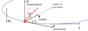
Figure 1: The local reference coordinate system used to derive the motion of the spin in the EM fields of the experiment. The vector $\hat{z}$ follows the momentum of the muon and $\hat{y}$ always points along the longitudinal direction defined by the main solenoid magnetic field $B_{y}$.

Using equation (1) and assuming that $\vec{\beta}\cdot\vec{E}=0$ and $\vec{\beta}\cdot\vec{B}=0$ the angle of spin precession around the radial axis due to a non-zero EDM is:

$$\Theta(t)=\Omega^{\mathchoice{}{}{\scriptscriptstyle}{}\text{EDM}}_{\hat{x}}t=\frac{\eta}{2}\frac{e}{m_{0}}\beta_{z}B_{y}t,$$ (2)

where $t$ is the elapsed time between the injection of the muon into the longitudinal magnetic field and its decay.

The relationship between the dimensionless parameter $\eta$ that characterizes the spin precession and the EDM $d$ is given by:

$$d=\frac{e\hslash}{4m_{0}c}\eta.$$ (3)

Combining (2) and (3) gives an expression of the rate of change of the angle of rotation of the spin $\dot{\Theta}$ as a function of the EDM $d$:

$$\dot{\Theta}=\frac{2c}{\hslash}\beta_{z}B_{y}d.$$ (4)

For the precursor and final experiments $\beta_{z}=0.26$ and $0.77$ respectively and $B_{y}=3$ T, hence, the angular velocities are

$$\dot{\Theta} =21.15\text{ \textmu rad/\textmu s},\text{ for }d=3\times 10^{-21}\leavevmode\nobreak\ e\cdot\text{cm and}$$ (5)

$$\dot{\Theta} =1.26\text{ \textmu rad/\textmu s},\text{ for }d=6\times 10^{-23}\leavevmode\nobreak\ e\cdot\text{cm}.$$ (6)

In the following sections we will discuss various effects with the goal of deriving the full description of the spin’s motion in the EM fields of the system. The derived equations can be used to place limits on measurement parameters such that the angular velocity of the spin precession due to the MDM is less than the experimental sensitivities shown in (5) and (6).

4 Sources of real spin precession

One of the large sources of a false EDM signal are oscillations and rotations of the spin due to the coupling of the MDM of the muon with the electric and magnetic fields present in the experimental setup. As a starting point we will describe analytically the motion of the spin due to the combined effect of ideal approximations of the magnetic field of the solenoid, the weakly focusing field and the electric field used in the frozen-spin method. The magnetic field of the solenoid is approximated as a uniform magnetic field oriented along the $\hat{y}$ axis. The weakly focusing field is described by the approximated field that is generated by a circular coil. The electric field is assumed to be a radial field generated from the potential difference between two infinite coaxial cylindrical electrodes. Some possible and important imperfections of these fields and their effect on the spin precession is discussed.

4.1 Spin precession along the radial axis

Assuming the particles follow a trajectory with a constant radius $\rho$, the radial magnetic field $B_{x}(y)$ of a cylindrical coil with $N$ turns and radius $R$ along that trajectory can be approximated with Murgatroyd1991 :

$$B_{x}(y)=\frac{3}{2}\mu_{0}NIR^{2}\frac{\rho y}{\left(R^{2}+y^{2}\right)^{\frac{5}{2}}},$$ (7)

where $I$ is the current passing through the coil and $\mu_{0}$ is the magnetic permittivity of vacuum. Expanding (7) in a Taylor series one obtains:

$$B_{x}(y)=\Phi_{0}\rho y-\frac{5}{2}\frac{\Phi_{0}}{R^{2}}\rho y^{3}+\mathcal{O}(y^{5}),\text{ where }\Phi_{0}=\frac{3}{2}\frac{\mu_{0}NI}{R^{3}}.$$ (8)

The longitudinal position of a particle with charge $e$, mass $m_{0}$ and velocity $c\vec{\beta}$ is given by the solution of:

$$\ddot{y}=\frac{1}{\gamma m_{0}}\left(eE_{y}+c\beta_{z}B_{x}(y)\right),$$ (9)

where we assume a constant non-zero longitudinal component of the electric field. The solution of the differential equation is the harmonic oscillator:

$$y(t)=y_{0}\cos(\omega_{\beta}t+\varphi)+\frac{1}{\Phi_{0}\rho}\frac{E_{y}}{c\beta_{z}},$$ (10)

$$\text{where }\omega_{\beta}=\sqrt{\Phi_{0}\frac{ec\beta_{z}}{\gamma m_{0}}\rho}$$ (11)

is the angular velocity of the vertical betatron oscillations (VBO).

For the precursor experiment where $\beta=0.258$ and $\gamma=1.03$ the period $T=2\pi/\omega_{\beta}$ of the VBO is approximately 600 ns. Note that this period depends only on the strength of the focusing field and the radial position of the muon. It does not depend on the momentum of the muon.

The precession of the spin due to the coupling of the MDM with the radial magnetic field due to the weakly focusing field is:

$$\left(\vec{\Omega}_{\mathchoice{}{}{\scriptscriptstyle}{}\text{MDM}}^{\mathchoice{}{}{\scriptscriptstyle}{}\text{WF}}\right)_{x}=-\frac{ea}{m_{0}}B_{x}(y(t))=\\ =-\frac{ea}{m_{0}}\left[\Phi_{0}\cos(\omega_{\beta}t+\phi_{0})\rho y_{0}-\frac{1}{c\beta_{z}}E_{y}\right].$$ (12)

The other source of radial precession that has to be considered is the radial magnetic field in the reference frame of the muon due to the non-zero longitudinal electric field in the laboratory reference frame. Using the T-BMT equation and taking only the radial component of the spin precession due to the electric field one obtains:

$$\left(\vec{\Omega}_{\mathchoice{}{}{\scriptscriptstyle}{}\text{MDM}}^{\scriptscriptstyle{}E_{y}}\right)_{x}=-\frac{e}{m_{0}c}\left(a-\frac{1}{\gamma^{2}-1}\right)\beta_{z}E_{y}.$$ (13)

Combining (12) and (13), for the total angular velocity of the radial precession due to the MDM around the $\hat{x}$ axis, one obtains :

$$\left(\vec{\Omega}_{\mathchoice{}{}{\scriptscriptstyle}{}\text{MDM}}\right)_{x}=-\frac{ea}{m_{0}}\left[\frac{1}{c}\left(1-\frac{1}{a(\gamma^{2}-1)}-\frac{1}{\beta^{2}_{z}}\right)\beta_{z}E_{y}\right.+\\ \left.\Phi_{0}\cos(\omega_{\beta}t+\phi_{0})\rho y_{0}\right].$$ (14)

4.2 Azimuthal spin precession

When the muons circulate in the storage ring they oscillate around an equilibrium orbit. Because of this oscillation the momentum of the particle is not at all times perpendicular to the longitudinal magnetic field leading to a non-zero projection of the magnetic field along its trajectory. This field is proportional to the angle between the muon momentum and the magnetic field $\delta=\angle(\vec{\beta},\vec{B})$. In turn, $\cos(\delta)=p_{y}/p_{z}$ and $p_{y}$ oscillates as $p_{y}=p_{y_{0}}\sin(\omega_{\beta}t)$. Thus:

$$B_{z}(t)=B_{y}\cos(\delta)\approx\frac{p_{y_{0}}}{p_{z}}\sin(\omega_{\beta}t)B_{y}.$$ (15)

The momentum $p_{y_{0}}$ is the momentum in the $\hat{y}$ direction when the muon is on the equilibrium orbit. It can be calculated as:

$$p_{y_{0}}=ec\beta\Phi_{0}\rho y_{0}\int_{0}^{\frac{\pi}{2\omega_{\beta}}}\cos(\omega_{\beta}t)dt=ec\beta\Phi_{0}\rho y_{0}\frac{1}{\omega_{\beta}}.$$ (16)

In the ideal case $\vec{\beta}=\lvert\beta\rvert\hat{z}$ and $\vec{E}=\lvert E\rvert\hat{x}$, but as the muons oscillate in the weakly focusing field there will be a non-zero $\hat{y}$ component of the velocity, thus:

$$\beta_{y}=(p_{y_{0}}/p_{z})\,\beta_{z}\sin(\omega_{\beta}t).$$ (17)

If the radial electric field $E_{x}$ is correctly set to the value $E_{f}$ required by the frozen-spin technique, then there will be no oscillations around the $\hat{z}$ axis, excluding the second order $\beta\cdot\vec{B}$ term in (1). At this value for the freeze field, it will counteract the precession induced by coupling of the MDM to the longitudinal field of the solenoid. However, if $E_{x}\neq E_{f}$ there will be imperfect cancellation of the $g-2$ precession around $\hat{z}$ which is proportional to the excess electric field $E_{ex}=E^{(\text{real})}-E^{(\text{freeze})}$ that the muon is subjected to:

$$\left(\vec{\Omega}_{\mathchoice{}{}{\scriptscriptstyle}{}\text{MDM}}^{\scriptscriptstyle E_{ex}}\right)_{z}=-\frac{e}{m_{0}c}\left(a-\frac{1}{\gamma^{2}-1}\right)\beta_{y}E_{\text{ex}}.$$ (18)

Considering (15), the angular velocity of the spin precession along the $\hat{z}$ axis due to the $\vec{\beta}\cdot\vec{B}$ term in the T-BMT equation is:

$$\left(\vec{\Omega}_{\mathchoice{}{}{\scriptscriptstyle}{}\text{MDM}}^{\,\scriptscriptstyle\beta\cdot B}\right)_{z}=\frac{ea}{m_{0}}\left(\frac{\gamma-1}{\gamma}\right)B_{z}(t).$$ (19)

Combining equations (19) and (18) gives the total angular velocity of the precession due to the MDM around the $\hat{z}$ axis:

$$\left(\vec{\Omega}_{\mathchoice{}{}{\scriptscriptstyle}{}\text{MDM}}\right)_{z}=-\frac{e}{m_{0}}\frac{p_{y_{0}}}{p_{z}}\sin\left(\omega_{\beta}t\right)\times\\ \left[\left(a-\frac{1}{\gamma^{2}-1}\right)\frac{\beta_{z}}{c}E_{ex}-a\left(\frac{\gamma-1}{\gamma}\right)B_{y}\right].$$ (20)

4.3 Electric field imperfections

The value of $E^{(\text{real})}$ may not be constant throughout the orbit of the muon if the central axes of the magnetic and electric fields are displaced or inclined with respect to each other. To obtain the components of the electric field with respect to the central axis of the solenoid, first consider a purely radial electric field created by perfect coaxial cylindrical electrodes with radii $A$ and $B$. In the reference frame $(x^{\prime},y^{\prime},z^{\prime})$ of the electrodes, where $z^{\prime}$ is parallel to the central axis of the electrodes, the field is given by:

$$\vec{E}^{\prime}(\vec{r})=\frac{V}{\log{\frac{B}{A}}}\begin{pmatrix}x^{\prime}/r^{2}\\ y^{\prime}/r^{2}\\ 0\\ \end{pmatrix},$$ (21)

where $r^{2}=(x^{\prime})^{2}+(y^{\prime})^{2}$. The electrode central axis, however, may be displaced and rotated with respect to the reference frame defined by the solenoid central axis. The electric field $\vec{E}$ in the reference frame of the solenoid can be obtained by transforming $\vec{E}^{\prime}$ as:

$$\vec{E}=R_{y}(\alpha)\vec{E}^{\prime}(R_{y}^{-1}(\alpha)\vec{r}+\vec{r}_{0}),$$ (22)

where $\vec{r}_{0}=(x^{\prime}_{0},y^{\prime}_{0},0)$ is the displacement between the two fields. $R_{y}(\alpha)$ is the rotation around the $y^{\prime}$ axis at an angle $\alpha$, where $\alpha$ is the angle between the central axis of the cylindrical electrodes and the central axis of the longitudinal magnetic field. Note here that due to the rotational symmetry of the fields we can always choose the reference frame to be such that arbitrary displacements can be represented in this way. The electric field in the reference frame defined by the longitudinal magnetic field is then:

$$\vec{E}(\vec{r})=V_{0}\begin{pmatrix}\frac{\xi}{\rho^{2}}\cos\alpha\\ \frac{\upsilon}{\rho^{2}}\\ -\frac{\xi}{\rho^{2}}\sin\alpha\end{pmatrix}$$ (23)

where $V_{0}=V/\log{(B/A)}$, $\upsilon=y^{\prime}+y^{\prime}_{0}$, $\xi=x^{\prime}_{0}+x^{\prime}\cos\alpha-z^{\prime}\sin\alpha$ and $\rho^{2}=\xi^{2}+\upsilon^{2}$.

The average of the radial electric field over the circular orbit of the muon can be obtained if $E^{\prime}$ is represented in cylindrical coordinates $(\rho,\phi,\zeta)$ as:

$$\left\langle E(\rho,\zeta)\right\rangle=\frac{1}{2\pi}\int_{0}^{2\pi}Ed\phi,$$ (24)

where $\rho$ is the radius of the orbit of the muon as a function of the magnetic field and the momentum of the particle, and $\zeta$ is parallel to $\hat{y}$.

The radial electric field the muon experiences in its reference frame is modeled as:

$$E^{(\text{real})}=\left\langle E(\rho,\zeta)\right\rangle_{\rho}+\frac{1}{2}\left(E_{\rho,max}-E_{\rho,min}\right)\cos(\omega_{c}t+\beta_{0}),$$ (25)

where $\omega_{c}=-eB_{y}/\gamma m_{0}$ is the cyclotron angular velocity, $E_{max}$ and $E_{min}$ are the maximal and minimal value of the electric field over one rotation of the muon and $\beta_{0}$ is the initial phase of the muon position along the orbit.

Note, (24) is valid only in the case of a circular orbit. In this case it can be shown numerically that:

$$\left\langle E(\rho,\zeta)\right\rangle=\left\langle E^{\prime}(\rho,\zeta)\right\rangle,$$ (26)

i.e., the rotation of the anode or cathode with respect to the muon orbit does not influence the average frozen spin condition and, more importantly, does not change the net E-field component in the $\hat{y}$ direction. As the centripetal force due to the B-field is $\approx 10^{3}$ higher than that due to the E-field and the expected misalignments between the center of the orbit and the center of the inner electrode are small, the circular orbit approximation holds well.

4.4 Combined spin precession

The initial orientation of the spin $\vec{S}=(S_{x},S_{y},S_{z})$ in spherical coordinates is:

$$\phi_{0}=\arctan\left(\frac{S_{x}}{S_{z}}\right),\quad\Theta_{0}=\arctan\left(\frac{\sqrt{S^{2}_{x}+S^{2}_{z}}}{S_{y}}\right)-\frac{\pi}{2}.$$ (27)

If there is an imperfect cancellation of the $g-2$ precession then there will be a rotation of the spin around the $\hat{y}$ axis. Thus, the angular velocity of the spin precession around $\hat{x}$ and $\hat{z}$ will be a projection of (20) and (33) along $\hat{y}$:

$$\lvert\vec{\Omega}_{\mathchoice{}{}{\scriptscriptstyle}{}\text{MDM}}\cdot\hat{y}\rvert=\left(\vec{\Omega}_{\mathchoice{}{}{\scriptscriptstyle}{}\text{MDM}}\right)_{x}\cos(\omega_{y}t+\phi_{0})+\left(\vec{\Omega}_{\mathchoice{}{}{\scriptscriptstyle}{}\text{MDM}}\right)_{z}\sin(\omega_{y}t+\phi_{0}),$$ (28)

where $\omega_{y}$ is the angular velocity of the precession around $\hat{y}$ due to the $g-2$ precession and is:

$$\omega_{y}=\frac{ea}{m_{0}}\frac{E_{\text{ex}}}{E_{f}}B_{y}.$$ (29)

In practice, $E_{\text{ex}}$ will oscillate (see (25)) with the cyclotron frequency due to the changing distance between the muon and the E-field center. The longitudinal B-field $B_{y}$ will oscillate with the VBO frequency due to the changing longitudinal component of the weakly focusing field (proportional to (7)). In a well tuned frozen-spin experiment $\omega_{y}$ is much lower than $\omega_{\beta}$ and $\omega_{c}$, and in this derivation the rotation of the spin around $\hat{y}$ is approximated with a constant angular velocity using the average values of $E_{\text{ex}}$ and $B_{y}$.

The total longitudinal rotation of the spin $\Theta$ is:

$$\Theta(t)=\int_{0}^{t}\lvert\Omega_{\mathchoice{}{}{\scriptscriptstyle}{}\text{MDM}}\cdot\hat{y}\rvert dt$$ (30)

Calculating (30) for the $\hat{z}$ component only one obtains:

$$\begin{split}\Theta_{z}(t)&=-\frac{e}{m_{0}}\mathop{{\int}}_{0}^{t}\left[\frac{p_{y_{0}}}{p_{z}}\left(\frac{\beta_{z}}{c}\left(a-\frac{1}{\gamma^{2}-1}\right)E_{\text{ex}}\right.\right.\\ &-\left.\left.a\left(\frac{\gamma-1}{\gamma}\right)B_{y}\right)\sin(\omega_{\beta}t^{\prime})+aB_{z}\right]\sin(\omega_{y}t^{\prime}+\phi_{0})dt^{\prime}\end{split}$$ (31)

Noting that:

$$\int_{0}^{t}\sin(\omega_{\beta}t^{\prime})\sin(\omega_{y}t^{\prime}+\phi_{0})dt^{\prime}\approx\\ -\frac{1}{\omega_{\beta}}\cos(\omega_{\beta}t)\sin(\omega_{y}t+\phi_{0}),\quad\text{if }\omega_{\beta}>>\omega_{y},$$ (32)

the oscillations due to the excess electric field along the $\hat{z}$ axis (along the momentum) and due to the non-zero $B_{z}$ magnetic field can be calculated by:

$$\begin{split}\Theta_{\hat{z}}(t)&=\frac{e}{m_{0}}\left[\frac{p_{y_{0}}}{p_{z}}\frac{1}{\omega_{\beta}}\cos\left(\omega_{\beta}t\right)\left(\frac{\beta_{z}}{c}\left(a-\frac{1}{\gamma^{2}-1}\right)E_{\text{ex}}\right.\right.\\ &-\left.\left.a\left(\frac{\gamma-1}{\gamma}\right)B_{y}\right)-\frac{1}{\omega_{y}}aB_{z}\right]\sin(\omega_{y}t+\phi_{0}).\end{split}$$ (33)

A similar calculation can be performed for the spin-precession along the $\hat{x}$ axis due to the radial magnetic field of the weakly focusing field:

$$\Theta_{\hat{x}}(t)=-\frac{ea}{m_{0}}\left[\frac{1}{\omega_{\beta}}\Phi_{0}\sin(\omega_{\beta}t+\phi_{0})\rho y_{0}\right]\cos(\omega_{y}t+\phi_{0}).$$ (34)

The spin-precession due to a non-zero electric field in the $\hat{y}$ direction can be easily integrated without approximations and gives:

$$\Theta_{\hat{z}\times\hat{y}}(t)=-\frac{ea}{m_{0}}\left[\left(1-\frac{1}{a(\gamma^{2}-1)}-\frac{1}{\beta_{z}^{2}}\right)\frac{\beta_{z}}{c}E_{y}\right]\times\\ \frac{1}{\omega_{y}}\sin(\omega_{y}t+\phi_{0}).$$ (35)

The total azimuthal angle $\Theta$ is the sum of the oscillations and rotations given above:

$$\Theta=\Theta_{\hat{x}}+\Theta_{\hat{z}}+\Theta_{\hat{z}\times\hat{y}}+\Theta_{0}.$$ (36)

Input parameters

The analytical equations have a few input parameters which can be roughly divided into two groups: stochastic initial conditions that vary for each particle in the storage ring at time $t_{0}$ of the experiment and constant or slowly changing parameters of the experimental system. The stochastic conditions in the first group are:

$$\vec{p}_{0} =(p_{x},0,p_{z})-\text{Initial momentum of the particle.}$$ (37)

$$\vec{S}_{0} =(S_{x},S_{y},S_{z})-\text{Initial spin of the particle.}$$

$$\vec{r}_{0} =(r_{x},r_{y},r_{z})-\text{Initial position of the particle.}$$

$$t_{0} -\text{Time after injection for which $p_{y}=0$.}$$

Note here, that the $p_{y}$ component is equal to zero as this is the defining moment when the particle is considered stored in the storage ring. The parameters $r_{x}$ and $r_{z}$ as well as $p_{x}$ and $p_{z}$ define the orbit of the muons and determine the electric field $E^{(\text{real})}$ to which they are subjected. The parameter $r_{y}$ is the starting position of the muon along the solenoid axis and defines the oscillations due to the radial weakly focusing magnetic field. The initial spin direction $\vec{S}_{0}$ determines the intermixing between the rotations around the $\hat{x}$ and $\hat{z}$ axes. There is also one constraint imposed on the spin orientation: $\lvert S_{0}\rvert=1$.

The parameters of the experimental system are:

1. $B_{y}$ – Main solenoid magnetic field strength.

2. $I,R,N$ – Current through the $N$ turns of the weakly focusing coils with radius $R$.

3. $V,b,a,\alpha$ – Voltage between the concentric cylinders with radii $b$ and $a$ defining the weakly focusing field. The angle $\alpha$ between the central axes of the electric field and solenoid magnetic field.

4. $p^{\scriptscriptstyle\text{(ideal)}}_{0}$ – Ideal momentum of the muons for which the freeze field is set.

5. $E_{y}$ – Constant electric field normal to the storage ring plane.

Thus, the analytical equations depend on 8 free stochastic parameters and 10 constant parameters of the experimental system. These parameters completely define the dynamics of the spin inside this model of a storage ring.

4.5 Comparison with Geant4 spin tracking

In order to verify the analytical equations a model of the experiment was developed using the Geant4 Monte Carlo simulation toolkit Agostinelli2003 . The EM fields of the experiment can be either calculated analytically or interpolated from field maps. The field maps are generated by ANSYS Maxwell finite element modeling (FEM) software. The simulation has three major EM field components:

1. The main solenoid magnetic field – constant value along $\hat{y}$ or field map supplied by FEM simulations.

2. Radial electric field given by (23) with a possibility to add a constant and uniform component in the longitudinal direction or FEM simulated field map.

3. Weakly focusing field modeled in ANSYS as a single circular coil with $R=65$ mm.

The muons start with zero momentum in the $\hat{y}$ direction as this is the initial condition for a stored muon. The simulation tracks the spin orientation in the reference frame of the muon and records it as a function of time. It can also track the direction with respect to a reference frame defined by the experimental setup, e.g., the solenoid.

A comparison between the derived analytical equations and the Geant4 spin tracking is shown in Figure 2. In the comparison a fine field map (0.2 mm step size) of the weakly focused field was used. All other EM fields are calculated analytically. The stepper used is the DormandPrinceRK78 routine Agostinelli2003 with $0.26$ mm step size. The stepping size was chosen so as to avoid effects due to resonances between the stepper and field map grids. The initial coordinates of the muon at the moment of storage were chosen arbitrarily (values specified in Figure 2 caption) for the purpose of the illustration. The electric field was set to such a value as to have imperfect cancellation of the $(g-2)$ precession. The anode coaxial E-field is tilted with respect to the longitudinal axis at $\alpha=0.01^{\circ}$ in order to highlight the cyclotron oscillations.

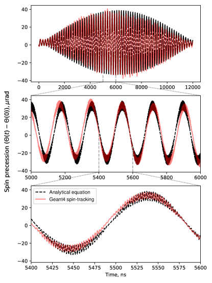
Figure 2: Comparison between the analytical equations (36) and the Geant4 spin tracking simulation. The initial parameters are arbitrarily set to $\vec{S}_{0}=(-0.89,0.00,-0.46)$, $\vec{p}_{0}=(0.84,0.00,0.55)\times 26.8$ MeV/c and $\vec{r}_{0}=(-16.95,5.00,22.10)$ mm. The ideal momentum for which the freeze field is set is $p_{0}^{\scriptscriptstyle\text{(ideal)}}=28.0$ MeV/c. The three subfigures show different timescales of the spin motion – uncompensated $(g-2)$ precession, betatron oscillations and cyclotron oscillations.

The comparison shows very good agreement between the analytical equations and the Geant4 spin tracking. The approximate equation for the description of the weakly focusing field (8) provides good estimates of the field strength and VBO frequency. The difference between the analytical and numerical approaches is less than 5 µrad sustained over 12 µs of simulation time, demonstrating the very good agreement between the two also when using realistic FEM generated field maps in Geant4.

5 Sources of apparent spin precession

If the muon spin has a component in the longitudinal direction then the probability for upstream $p_{u}$ and downstream $p_{d}$ ejected decay positrons will differ and an asymmetry $A$ will be observed:

$$A(t)=\frac{p_{u}-p_{d}}{p_{u}+p_{d}}=\sin\left(\Theta(t)\right)\alpha P\approx\Theta(t)\,\alpha P,$$ (38)

where $\alpha$ is the parity violating decay asymmetry averaged over the positron energy and $P$ is the initial polarization. Equation (38) is valid when $\Theta(t)\ll 1$, which is the case of EDM induced spin precession.

Using (2) and (38), the rate of change of the asymmetry $\dot{A}$ is:

$$\dot{A}=\frac{\eta}{2}\frac{e}{m_{0}}\beta_{z}B_{y}\alpha P.$$ (39)

We would require that the measured asymmetry $\dot{A}_{m}$ due to spurious EDM mimicking effects is $\dot{A}_{m}\ll\dot{A}$.

The number of detected positrons in the upstream detector $N_{u}$ is given by:

$$N_{u}=\Omega_{u}\varepsilon_{u}p_{u}D,$$ (40)

where $D$ is the total number of decayed muons, $\varepsilon_{u}$ is the detection efficiency for positrons and $\Omega_{u}$ is the solid angle coverage of the upstream detector. Both $\Omega_{u}$ and $\varepsilon_{u}$ can be summarized with a single parameter $\kappa_{u}=\Omega_{u}\varepsilon_{u}$ expressing the effective detection efficiency of the upstream detector. A similar equation can be given for the downstream detector and so:

$$N_{u}=\kappa_{u}p_{u}D=\kappa_{u}D_{u}\text{ and }N_{d}=\kappa_{d}p_{d}D.$$ (41)

From the point of view of the experiment, substituting equation (41) in (38), the measured asymmetry $A_{m}$ is given by:

$$A_{m}=\frac{1}{D}\left(\frac{N_{u}}{\kappa_{u}}-\frac{N_{d}}{\kappa_{d}}\right).$$ (42)

If the effective detection efficiencies $\kappa$ are constant in time no systematic effect appears, but a time dependence, e.g., by a disturbance of the detector electronics through the pulsed kicker field, leads to a systematic bias. A worst-case scenario assumption is the case where the kicker field disturbs the detection efficiency in both the upstream and downstream detectors in opposite directions and its effect reduces exponentially with time. The disturbance can be modeled as:

$$\kappa_{u}=\kappa_{u0}-\Delta_{\kappa}e^{-t/\tau_{k}}\text{ and }\kappa_{d}=\kappa_{d0}+\Delta_{\kappa}e^{-t/\tau_{k}},$$ (43)

where $\kappa_{u0}$ and $\kappa_{d0}$ are some equilibrium detection efficiencies, $\Delta_{\kappa}$ is the perturbation in the efficiency due to the kicker field and $\tau_{k}$ is the time-constant of its effect.

In order to quantify the false EDM signal that can be caused by time-dependent efficiency parameters let us assume that there is no true EDM signal and the upstream and downstream emission probabilities are equal $p_{u}=p_{d}$ leading to $D_{u}=D_{d}=D/2$. Then the observed asymmetry is:

$$A_{m}=\kappa_{u}-\kappa_{d}=\kappa_{u0}-\Delta_{\kappa}e^{-t/\tau_{k}}-\kappa_{d0}-\Delta_{\kappa}e^{-t/\tau_{k}}.$$ (44)

The measured EDM signal is given by the time derivative of the asymmetry, thus:

$$\dot{A}_{m}=\frac{2}{\tau_{k}}\Delta_{\kappa}e^{-t/\tau_{k}}.$$ (45)

From equation (45) we can observe that the systematic effect decreases with time $t$ as expected. The effect is exacerbated if $\tau_{k}$ is on the order of magnitude of the experimental measurement time $t$ which is several muon lifetimes. The limits on $\tau_{k}$ and $\Delta_{\kappa}$ can be derived by requesting that the measured false asymmetry $\dot{A}_{m}$ is lower than the theoretical prediction $\dot{A}$ from (39) for a given $\eta$.

6 Conclusions

Analytical equations for the description of the MDM precession in the EM fields of the experiment were derived. The equations were compared to a Geant4 Monte Carlo simulation using realistic field maps generated using the FEM software ANSYS Maxwell. Very good agreement has been observed between the two and the analytical equations seem to describe well the spin motion at short, medium and long timescales.

A method of calculation of the measured false EDM signal due to exponential changes in the positron detection efficiency is shown. If the detection efficiency is constant, even if different, for each detector for early-to-late times, then there would be no false EDM signal. A false EDM would be generated in the case of change in the detection efficiency of upstream relative to downstream detectors and the systematic effect is more prominent for time-constants on the order of the muon lifetime.

The presented methods will be used to derive limits on the mechanical production and EM field uniformity of the muon EDM experiments to be built at the PSI.

7 Acknowledgements

This work is financed by the Swiss National Science Fund under grant № 204118.

References

- (1) M. Pospelov, A. Ritz, Ann. Phys. 318, 119 (2005)
- (2) C.Y. Seng, Phys. Rev. C91, 025502 (2015), 1411.1476
- (3) B. Abi, T. Albahri, S. Al-Kilani, D. Allspach, L. Alonzi, A. Anastasi, A. Anisenkov, F. Azfar, K. Badgley, S. Baeßler et al., PRL 126 (2021)
- (4) W. Altmannshofer, P. Stangl, D.M. Straub, Phys. Rev. D 96, 055008 (2017), 1704.05435
- (5) B. Capdevila, A. Crivellin, S. Descotes-Genon, J. Matias, J. Virto, JHEP 2018, 93 (2018), 1704.05340
- (6) F.J.M. Farley, K. Jungmann, J.P. Miller, W.M. Morse, Y.F. Orlov, B.L. Roberts, Y.K. Semertzidis, A. Silenko, E.J. Stephenson, Physical Review Letters 93 (2004)
- (7) A. Adelmann, M. Backhaus, C.C. Barajas, N. Berger, T. Bowcock, C. Calzolaio, G. Cavoto, R. Chislett, A. Crivellin, M. Daum et al., Search for a muon EDM using the frozen-spin technique (2021), https://arxiv.org/abs/2102.08838
- (8) D. Barna, Phys. Rev. Accel. Beams 20 (2017)
- (9) H. Iinuma, H. Nakayama, K. Oide, K. ichi Sasaki, N. Saito, T. Mibe, M. Abe, Nucl. Instrum. Meth. A 832, 51 (2016)
- (10) G.W. Bennett et al. (Muon (g-2)), Phys. Rev. D80, 052008 (2009), 0811.1207
- (11) L.H. Thomas, The London, Edinburgh, and Dublin Philosophical Magazine and Journal of Science 3, 1 (1927)
- (12) B. Montague, Physics Reports 113, 1 (1984)
- (13) M.H. Tahar, C. Carli, Physical Review Accelerators and Beams 24 (2021)
- (14) I.I. Rabi, N.F. Ramsey, J. Schwinger, Rev. Mod. Phys. 26, 167 (1954)
- (15) P.N. Murgatroyd, American Journal of Physics 59, 949 (1991)
- (16) S. Agostinelli, J. Allison, K. Amako, J. Apostolakis, H. Araujo, P. Arce, M. Asai, D. Axen, S. Banerjee, G. Barrand et al., Nucl. Instrum. Meth. A 506, 250 (2003)