Topological dynamics of adiabatic cat states

Abstract

We consider a qubit topologically coupled to two quantum modes. We show that any initial separable state of this system generically evolves into an adiabatic cat state. Such a state is a superposition of two adiabatic states in which the qubit is entangled between the modes. The topological coupling between the qubit and the modes gives rise to the separation in energy between these two components which evolve into states with distinguishable energy content.

Traditionally, a pump is a device that transfers energy from a source - an engine - to a fluid. The transfer is achieved through a suitably designed mechanical coupling. Topological pumping is a modern extension of such a device. The first historical example of such a topological pump was provided by Thouless who considered a periodically modulated in time one dimensional crystal [1], realized experimentally in various forms [2, 3, 4, 5, 6, 7, 8, 9, 10, 11, 12, 13]. A simpler realization was provided recently in the form of a qubit driven at two different frequencies [14], later extended to more complex driven zero dimensional devices [15, 16, 17, 18, 19, 20, 21]. These studies discussed pumping through the dynamics of the pump described as a driven quantum system. Indeed the slow and periodically modulated parameters generates a quantized current either through the quantum system, or,in the last case, in an abstract space of harmonics of the drives. This current thereby effectively describes a transfer between the drives.

In this paper, we reconcile the description of such a topological device with that of traditional pumps by considering on equal footing the qubit and the drives. This amounts to describe these drives quantum mechanically instead of classical parameters. We model them as quantum modes, characterized by a pair of conjugated operators accounting for their phase and number of quanta. This extends previous mixed quantum-classical descriptions of the drives [22, 23, 24]. We focus on the regime of adiabatic dynamics in which these quantum modes are slow compared to the qubit, neglecting effects induced by a faster drive, recently discussed in the context of topological Floquet systems [25, 26, 27, 28, 27, 29, 30, 31].

The dynamics of a system with slow and fast degrees of freedom has been largely studied in terms of an effective Hamiltonian [32, 33, 34]. Here we focus on the adiabatically evolved quantum states. Our quantum mechanical description shows that an initial separable state generically evolves into a superposition of two components. Each component is an adiabatic state of the driven qubit. The topological nature of the coupling between the qubit and the modes splits these two components apart in energy: for each component, an energy transfer occurs between the two quantum modes, in opposite directions for the two components. This topological dynamics effectively creates an adiabatic cat states: a superposition of two quantum adiabatic states distinguishable through measures of the modes’ energy. Besides, we show that in each of the component of this cat state, the qubit is entangled with the two modes. The origin of this entanglement lies in the geometrical properties of the coupling at the origin of the topological pumping. Hence a topological coupling necessarily entangles a pump with its driving modes.

Interestingly, similar qubit-modes quantum systems were recently proposed [35] and experimentally realized in quantum optical devices [36] to simulate topological lattice models. In this context, the Hamiltonians of a qubit coupled to cavities was expressed in terms of Fock-state lattices, and shown, with two cavities, to realize a chiral topological phase [37, 38], and , with three cavities, the quantum or valley Hall effect [35, 39]. Indeed the focus of these realizations was on synthetic topological models and their associated zero-energy states. Our approach bridges the gap between the study of topological pumping of driven systems and these studies of quantum optical devices.

Our paper is organized as follows. In Sec. I we introduce the model of a qubit driven by two quantum modes (Sec. I.1) and discuss qualitatively the typical dynamics of adiabatic cat states (Sec. I.2). In Sec. II we characterize the two components of the cat states as adiabatic states and identify their effective dynamics which splits them apart in energy. We characterize the weight of each cat component for a separable initial state. In Sec. III we study each cat component, relating the entanglement between the qubit and the modes to the quantum geometry of the adiabatic states (Sec. III.1), and discussing the evolution of the number of quanta of each mode in relation with Bloch oscillations and Bloch breathing (Sec. III.2).

I A qubit driven by two quantum modes

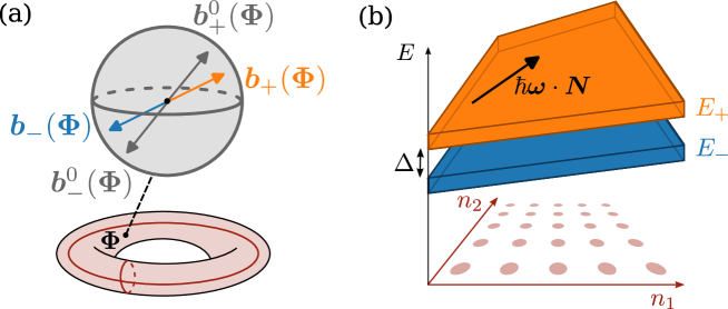
Figure 1: Phase and number representations of a quantum qubit-2 modes model. (a) Phase representation, convenient to represent the dynamics of the qubit. At each value of the phases $\bm{\Phi}$ are associated qubit eigenstates $\ket{\psi_{\pm}^{0}(\bm{\Phi})}$ represented by a vector $\bm{b}_{\pm}^{0}(\bm{\Phi})=\pm\bm{h}(\bm{\Phi})/|\bm{h}(\bm{\Phi})|$ on the Bloch sphere (in grey). The adiabatic states $\ket{\psi_{\pm}(\bm{\Phi})}$, represented by a vector $\bm{b}_{\pm}(\bm{\Phi})$, are a perturbative deformation of the eigenstates. (b) Number representation, convenient to represent the dynamics of the modes. In this viewpoint the model can be interpreted as an unusual model of spin-half particle on a discrete lattice where $\bm{N}=(n_{1},n_{2})\in\mathbb{Z}^{2}$ represents its position on the lattice and $\bm{\Phi}\in[0,2\pi]^{2}$ the Bloch momenta. This particle is submitted to an electric field $\hbar\bm{\omega}\cdot\hat{\bm{N}}$ and a strong spin-orbit coupling $\bm{h}(\hat{\bm{\Phi}})\cdot\bm{\sigma}$. As a consequence, the adiabatic states are associated to energy bands $E_{\pm}$ tilted in the direction $\bm{\omega}$ of the electric field and separated by the gap $\Delta$ due to the spin-orbit coupling.

I.1 Model

We consider the dynamics of two quantum modes coupled to a fast quantum degree of freedom, chosen for clarity as a two level system, a qubit. Each slow mode is described by a phase operator $\hat{\phi}_{i}$ of continuum spectrum $[0,2\pi]$, conjugated to a number operator $\hat{n}_{i}$ of discrete spectrum $\mathbb{Z}$, such that $[\hat{n}_{i},\hat{\phi}_{j}]={\rm i}\delta_{ij}$ [40]. We assume that the fast degree of freedom couples only to the phases of the modes, through a Hamiltonian $H(\hat{\bm{\Phi}})$ with $\hat{\bm{\Phi}}=(\hat{\phi}_{1},\hat{\phi}_{2})$. Noting $\bm{\omega}=(\omega_{1},\omega_{2})$ the frequencies of the modes, and $\hat{\bm{N}}=(\hat{n}_{1},\hat{n}_{2})$ their respective number operators, the dynamics of the full quantum system is governed by the Hamiltonian

$$\hat{H}_{\rm tot}=\hbar\bm{\omega}\cdot\hat{\bm{N}}\otimes\mathbb{I}+H(\hat{\bm{\Phi}})\,,\ H(\hat{\bm{\Phi}})=\sum_{\alpha=1}^{3}h_{\alpha}(\hat{\bm{\Phi}})\otimes\sigma_{\alpha}\,.$$ (1)

Such a model appears as the natural quantization of a $2$-tone Floquet systems, where the time-dependant parameters $\phi_{i}(t)=\omega_{i}t$ of the qubit Hamiltonian $\bm{h}(\phi_{1}(t),\phi_{2}(t))\cdot\bm{\sigma}$ are here considered as true quantum degrees of freedom. Note that we will focus on the adiabatic dynamics of such a Floquet model, valid for slow frequencies $\hbar\omega_{i}$ compared with the qubit’s spectral gap $2|\bm{h}|$. Physically, the two modes of model (1) often results from the coupling to a harmonic oscillator [35, 22, 37, 24]. Describing this oscillator by a pair of conjugated operators $\hat{n}_{i},\hat{\phi}_{i}$ is valid for states with a number of quanta $\bar{n}$ large compared to any dynamical variation of and spreading of $n$, $\Delta n\ll\bar{n}$ [22].

The modes’ intrinsic energies depend on the number of quanta $\bm{N}$ while the qubit’s energy depend on their phases: hence we will use two dual representations of the dynamics of the system through this paper. When focusing on the qubit’s evolution, the phase representation is natural, represented in Fig. 1(a): at each value of the phases $\bm{\Phi}$ are associated qubit’s eigenstates $\ket{\psi_{\pm}^{0}(\bm{\Phi})}$. The modes’ dynamics translate into an evolution with time of the phase, and thus an evolution of the associated qubit’s states $\ket{\psi_{\pm}(\bm{\Phi})}$ which slightly differ from the eigenstates and will be discussed in section II.1.

Focusing on the quantum modes, their dynamics is conveniently represented in number representation, Fig. 1(b). In this viewpoint, we can interpret the model as that of a particle on a 2D lattice of sites $\bm{N}=(n_{1},n_{2})$, $\bm{\Phi}=(\phi_{1},\phi_{2})$ being the associated Bloch momenta in the first Brillouin zone. The Hamiltonian (1) describes its motion, submitted to both a spin-orbit coupling $H(\hat{\bm{\Phi}})$ and an electric field $\hbar\bm{\omega}$. We will use this analogy to relate the geometrical and topological properties of gapped phases on a lattice to those of the above quantum model. Note that in this case, there is no embedding of this lattice in $\mathbb{R}^{2}$ as opposed to the Bloch theory of crystals. The position operator identifies with coordinate operator on the lattice. As a consequence, there is no ambiguity in a choice of Bloch convention and definition of the Berry curvature [41, 42].

In the following, we consider a topological coupling between the qubit and the two quantum modes. This corresponds to the situation where the qubit remains gapped irrespective of the phase $\bm{\Phi}$ of the quantum modes, i.e. $|\bm{h(\bm{\Phi})}|\geq\Delta>0$ for all values of $\bm{\Phi}$. Besides, the topological nature of the drive originates from the condition that the map $\bm{\Phi}\in[0,2\pi]^{2}\to\bm{h(\bm{\Phi})}$ wraps around the origin in $\mathbb{R}^{3}$. This is a condition of strong coupling between the qubit and the drive. Indeed, if we represent the qubit’s eigenstates by a vector $\bm{b}_{\pm}^{0}(\bm{\Phi})=\pm\bm{h}(\bm{\Phi})/|\bm{h}(\bm{\Phi})|$ on the Bloch sphere, then any point of the sphere correspond to a ground state of the qubit for a particular phase state of the drive. This is in contrast with the familiar weak coupling limit where states around the south pole, $\ket{\downarrow}$, are associated to the ground states and those close to the north pole, $\ket{\uparrow}$, to excited states. In the present case, knowledge of the state of the qubit is not sufficient to determine whether it is in the excited or ground state: information on the state of the driving modes is necessary.

Throughout this paper, the numerical results are obtained by considering an example of such a topological coupling provided by the quantum version of the Bloch Hamiltonian of the half Bernevig-Hughes-Zhang (BHZ) model [43]:

$$h_{x}(\hat{\bm{\Phi}}) =\frac{\Delta}{2}\sin(\hat{\phi}_{1}),$$ (2a)

$$h_{y}(\hat{\bm{\Phi}}) =-\frac{\Delta}{2}\sin(\hat{\phi}_{2}),$$ (2b)

$$h_{z}(\hat{\bm{\Phi}}) =\frac{\Delta}{2}\left(1-\cos(\hat{\phi}_{1})-\cos(\hat{\phi}_{2})\right),$$ (2c)

where the parameter $\Delta>0$ is the gap of the qubit. See appendix F for details on the numerical method.

I.2 Topological dynamics of adiabatic of cat states

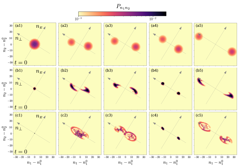
Figure 2: Typical dynamics of adiabatic cat states. Distribution of number of quanta of the two modes $P_{n_{1}n_{2}}=\bra{n_{1},n_{2}}\hat{\rho}_{12}\ket{n_{1},n_{2}}$ at different times for three initial states. The modes are prepared in a Gaussian state with an average value of phase $\phi_{1}^{0}=\phi_{2}^{0}=0$ and an equal width in number of quanta $\Delta n_{1}=\Delta n_{2}=\Delta n$, corresponding to a width $\Delta\phi=1/(2\Delta n)$ in phase. The qubit is prepared in $(\ket{\uparrow}+\ket{\downarrow})/\sqrt{2}$. The evolution of states with different initial width $\Delta n$ is represented: line (a), $\Delta n=5$, $\Delta\phi\simeq 0.03\pi$; line (b), $\Delta n=0.7$, $\Delta\phi\simeq 0.23\pi$, and line (c), Quasi-Fock state $\Delta n=1/(2\pi)$, delocalized in phase $\Delta\phi=\pi$. The columns (2) to (5) represent the time evolved state at respectively $t=8/3$, $16/3$, $8$ and $t=32/3$ in units of the period of the first mode $T_{1}=2\pi/\omega_{1}$. The dynamics splits the initial state in a cat state in the sense of a superposition of two states with distinguishable energy content.

In this section, we illustrate the topological dynamics of the system starting from a typical state. This dynamics is analyzed quantitatively in the remaining of this paper. We focus on separable initial state, easier to prepare experimentally:

$$\ket{\Psi(t=0)}=\ket{\chi_{1}}\otimes\ket{\chi_{2}}\otimes\ket{\psi_{q}}.$$ (3)

Each quantum mode is prepared in a Gaussian state $\ket{\chi_{i}}$, characterized by an average number of quanta $n_{i}^{0}$ and a phase $\phi_{i}^{0}=0$, with widths $\Delta n_{i},\Delta\phi_{i}$ satisfying $\Delta\phi_{i}\Delta n_{i}=\frac{1}{2}$. The qubit is prepared in a superposition $\ket{\psi_{q}}=(\ket{\uparrow_{z}}+\ket{\downarrow_{z}})/\sqrt{2}$.

We consider modes with frequency of the same order of magnitude, $\hbar\omega_{1}=0.075\Delta$ and $\omega_{2}/\omega_{1}=(1+\sqrt{5})/2\simeq 1.618$, such that in the following, time is arbitrarily expressed in unit of period of the first mode $T_{1}=2\pi/\omega_{1}$. In Fig. 2, we represent the dynamics of this state $\ket{\Psi(t)}$ by displaying the associated number distribution of the modes $P_{n_{1}n_{2}}(t)=\bra{n_{1},n_{2}}\hat{\rho}_{12}(t)\ket{n_{1},n_{2}}$, with $\hat{\rho}_{12}(t)$ the corresponding reduced density matrix of the modes. Three initial states with respective initial number width $\Delta n=\Delta n_{1}=\Delta n_{2}=5$, $\Delta n=0.7$ and $\Delta n=1/(2\pi)$ (quasi-Fock state delocalized in phase $\Delta\phi=\pi$) are shown respectively in Fig. 2 (a1), (b1) and (c1). The time evolved states at respectively $t=0,8/3,16/3,8$ and $t=32/3$ are represented respectively on columns 1 to 5 of Fig. 2. We observe a splitting of the initial state into a superposition of two states

$$\ket{\Psi(t)}=\ket{\Psi_{-}(t)}+\ket{\Psi_{+}(t)}.$$ (4)

The photon number distribution of $\ket{\Psi_{-}(t)}$ and $\ket{\Psi_{+}(t)}$ drift in opposite directions, corresponding to energy transfers between modes $1$ and $2$ in opposite directions. This drift is a manifestation of the topological pumping discussed in classical-quantum models [14, 23]. This pumping is conveniently represented by introducing rotated number coordinates

$$n_{\scriptscriptstyle E} =\frac{1}{|\bm{\omega}|}(\omega_{1}n_{1}+\omega_{2}n_{2}),$$ (5)

$$n_{\perp} =\frac{1}{|\bm{\omega}|}(-\omega_{2}n_{1}+\omega_{1}n_{2}),$$ (6)

with $|\bm{\omega}|=\sqrt{\omega_{1}^{2}+\omega_{2}^{2}}$. $n_{\scriptscriptstyle E}|\bm{\omega}|$ corresponds to the total energy of the modes and is constant up to the instantaneous energy exchange with the qubit. $n_{\perp}$ is the coordinate in the direction perpendicular to $\bm{\omega}$. A transfer of energy between mode 1 and mode 2 naturally translates into a drift in the $n_{\perp}$ direction, at fixed average $n_{\scriptscriptstyle E}$. We also observe that for small initial $\Delta n$, corresponding to lines (b) and (c), each component $\ket{\Psi_{-}(t)}$ and $\ket{\Psi_{+}(t)}$ undergoes a complex breathing dynamics around the drift. This oscillatory behavior is reminiscent of Bloch oscillations of the associated particle submitted to an electric field, superposed with a topological drift originating from the anomalous transverse velocity. After an initial time of separation, the number distributions for $\ket{\Psi_{-}(t)}$ and $\ket{\Psi_{+}(t)}$ no longer overlap (Fig. 2 columns 4 and 5). The system is then in a cat state: a superposition of two states with well distinguishable energy content.

We will now study quantitatively these cat states and their dynamics. In section II, we identify the two components $\ket{\Psi_{\pm}(t)}$ as adiabatic states (Sec. II.1). We study their topological dynamical separation into a cat state (Sec. II.2). We characterize the weight of each component of the cat (Sec. II.3) and identify a family of cat states with equal weight on each component. In section III.1 we analyze the entanglement between the qubit and the modes for each cat component, and relate it to the quantum geometry of the adiabatic states. Finally we discuss the dynamics of each cat component around the average drift, in relation with Bloch oscillations and Bloch breathing on the associated lattice (Sec. III.2).

II Adiabatic decomposition

II.1 Adiabatic projector

When the driving frequencies remain small compared to the qubit’s gap, $\hbar\omega_{i}\ll\Delta$, we naturally describe the effective dynamics of the coupled qubit and drives in terms of fast and slow quantum degrees of freedom. This is traditionally the realm of the Born-Oppenheimer approximation. Historically both degrees of freedom were those of massive particles, the slow modes being associated with the heavy nucleus of a molecule and the fast ones with the light electrons [44, 45, 32]. In this context, the Born-Oppenheimer approximation assumes that the time evolved state stays closed to the instantaneous eigenstates of the fast degrees of freedom and describes the resulting effective dynamics of the slow degree of freedom. The distinctive characteristic of the present quantum modes - qubit model from the usual Born-Oppenheimer setting is the linearity of the Hamiltonian (1) in the variable $\hat{\bm{N}}$. This allows to express in a simple form the corrections to the Born-Oppenheimer approximation for the adiabatic states. Let us explain the procedure to construct such states, while referring to appendix B for technical details.

We note $\ket{\bm{\Phi}}$ the eigenstates of the phase operator of the modes $\hat{\bm{\Phi}}$. Due to the linearity in $\hat{\bm{N}}$ of the Hamiltonian (1), the time evolution of a phase eigenstate $\ket{\bm{\Phi}}\otimes\ket{\psi}$, where $\ket{\psi}$ is a state of the qubit, is $\ket{\bm{\Phi}-\bm{\omega}t}\otimes U(t;\bm{\Phi})\ket{\psi}$. The time evolution operator $U$ is deduced from that for the Floquet model parametrized by classical phases $\bm{\omega}t$:

$$U(t;\bm{\Phi})=\mathcal{T}\exp\left[-\frac{{\rm i}}{\hbar}\int_{0}^{t}\differential\tau~{}H(\bm{\Phi}-\bm{\omega}\tau)\right]\ ,$$ (7)

where $\mathcal{T}$ denotes time ordering.

Adiabatic projector of the qubit.

We denote by $\ket{\psi^{0}_{\nu}(\bm{\Phi})}$, $\nu=\pm$, the normalized eigenstates of the two-level driven Hamiltonian $H(\bm{\Phi})\ket{\psi_{\nu}^{0}(\bm{\Phi})}=\nu|\bm{h}(\bm{\Phi})|\ket{\psi_{\nu}^{0}(\bm{\Phi})}$ for each $\bm{\Phi}$ in $[0,2\pi]^{2}$. For small frequencies $\omega_{i}$, given the time evolution of phase eigenstates, we can reasonably expect that the coupled qubit-modes system prepared in an eigenstate $\ket{\bm{\Phi}}\otimes\ket{\psi_{\nu}^{0}(\bm{\Phi})}$ will remain in a translated eigenstate. However this simple picture is only qualitatively valid: eigenstates get hybridized by adiabatic dynamics, even at arbitrarily small driving frequencies. As a consequence, we identify the family of adiabatic states $\ket{\psi_{\nu}(\bm{\Phi})}$ such that the dynamics occurs within each family of states $\ket{\bm{\Phi}}\otimes\ket{\psi_{\nu}(\bm{\Phi})}$. Adiabatic evolution is then represented as a transport from $\ket{\bm{\Phi}}\otimes\ket{\psi_{\nu}(\bm{\Phi})}$ to $\ket{\bm{\Phi}^{\prime}}\otimes\ket{\psi_{\nu}(\bm{\Phi}^{\prime})}$ within this family, indexed by translations of $\bm{\Phi}\to\bm{\Phi}^{\prime}=\bm{\Phi}-\bm{\omega}t$.

In practice, the adiabatic states $\ket{\psi_{\nu}(\bm{\Phi})}$ are conveniently determined from the adiabatic projector $\pi_{\nu}(\bm{\Phi})=\ket{\psi_{\nu}(\bm{\Phi}}\bra{\psi_{\nu}(\bm{\Phi})}$ [46, 47]. Introducing the dimensionless perturbative parameter $\epsilon$ by $\bm{\omega}=\epsilon\bm{\Omega}$, $\pi_{\nu}(\bm{\Phi})$ is defined as a series in $\epsilon$: $\pi_{\nu}(\bm{\Phi})=\sum_{k}\epsilon^{k}\pi_{\nu,k}(\bm{\Phi})$. Stability of each family of adiabatic states under the dynamics amounts to impose the condition

$$U(t;\bm{\Phi})\pi_{\nu}(\bm{\Phi})U(t;\bm{\Phi})^{\dagger}=\pi_{\nu}(\bm{\Phi}-\bm{\omega}t)\,,$$ (8)

where the evolution operator is defined in (7). Solving order by order in $\epsilon$ for this equation, together with the constituting property of a projector $\pi^{2}_{\nu}(\bm{\Phi})=\pi_{\nu}(\bm{\Phi})$, leads to the solution at order $0$: $\pi_{\nu,0}(\bm{\Phi})=\ket{\psi_{\nu}^{0}(\bm{\Phi})}\bra{\psi_{\nu}^{0}(\bm{\Phi})}$ and to first order

$$\pi_{\nu,1}(\bm{\Phi})=\\ \sum_{\mu\neq\nu}\ket{\psi_{\mu}^{0}(\bm{\Phi})}\frac{\sum_{i}\hbar\omega_{i}A_{\mu\nu,i}^{0}(\bm{\Phi})}{E_{\mu}^{0}(\bm{\Phi})-E_{\nu}^{0}(\bm{\Phi})}\bra{\psi_{\nu}^{0}(\bm{\Phi})}+\mathrm{h.c.}$$ (9)

with $A_{\mu\nu,i}^{0}(\bm{\Phi})=i\innerproduct{\psi_{\mu}^{0}(\bm{\Phi})}{\partial_{\phi_{i}}\psi_{\nu}^{0}(\bm{\Phi})}$ the components of the non-abelian Berry connection of the eigenstates, and $E_{\pm}^{0}(\bm{\Phi})=\pm|\bm{h}(\bm{\Phi})|$ the eigenenergies.

Adiabatic grading of the Hilbert space.

The above adiabatic decomposition of the qubit states allows for a natural decomposition of all states of the qubit-modes system. We proceed by extending the adiabatic projector of the qubit $\pi_{\nu}(\bm{\Phi})$ to a the projector acting on the Hilbert space of the whole system

$$\hat{P}_{\nu}=\int\differential\bm{\Phi}~{}\ket{\bm{\Phi}}\bra{\bm{\Phi}}\otimes\pi_{\nu}(\bm{\Phi})\ ,\ \nu=\pm\ .$$ (10)

This projector provides a decomposition of any qubit-mode state $\ket{\Psi}$ into two adiabatic states

$$\ket{\Psi}=\ket{\Psi_{-}}+\ket{\Psi_{+}}\ ,\ \ket{\Psi_{\nu}}=\hat{P}_{\nu}\ket{\Psi}\,,\ \nu=\pm\ .$$ (11)

For a separable initial state (3), each adiabatic component $\ket{\Psi_{\nu}}$ is characterized by a wave amplitude $\chi_{\nu}(\bm{\Phi})$ according to

$$\ket{\Psi_{\nu}} =\int\differential^{2}\bm{\Phi}~{}\chi_{\nu}(\bm{\Phi})\ket{\bm{\Phi}}\otimes\ket{\psi_{\nu}(\bm{\Phi})}\ ,$$ (12)

$$\chi_{\nu}(\bm{\Phi}) =\chi(\bm{\Phi})\innerproduct{\psi_{\nu}(\bm{\Phi})}{\psi_{q}}\ .$$ (13)

with $\chi(\bm{\Phi})=\innerproduct{\phi_{1}}{\chi_{1}}\innerproduct{\phi_{2}}{\chi_{2}}$ the wavefunction of the modes in the initial state (3). This splits the total Hilbert space $\mathcal{H}_{\rm tot}$ in two adiabatic subspaces  $\mathcal{H}_{\rm tot}=\mathcal{H}_{-}\oplus\mathcal{H}_{+}$, where $\mathcal{H}_{-}$ and $\mathcal{H}_{+}$ are respectively the images of the projectors $\hat{P}_{-}$ and $\hat{P}_{+}$.

Topology of the family of adiabatic states.

The ensemble of adiabatic states $\ket{\psi_{\nu}(\bm{\Phi})}$ parametrized by the classical configuration space $\bm{\Phi}\in[0,2\pi]^{2}$ defines a vector bundle. This vector bundle is a smooth deformation of the eigenstates bundles $\ket{\psi^{0}_{\nu}(\bm{\Phi})}$ associated to a spectral projector (Fig. 1(a)). As a consequence, the local curvature associated with the adiabatic bundle

$$F_{\nu}(\bm{\Phi})=i\innerproduct{\partial_{\phi_{1}}\psi_{\nu}(\bm{\Phi})}{\partial_{\phi_{2}}\psi_{\nu}(\bm{\Phi})}-(1\leftrightarrow 2),$$ (14)

differs from the canonical Berry curvature associated with the eigenstates bundle [48]. The curvature (14) generalizes the Berry curvature to all orders in the adiabatic parameter $\epsilon$, in a similar way that the Aharonov-Anandan phase [49] generalizes the Berry phase. On the other hand, the Chern number ${\mathcal{C}}_{\nu}$ of both bundles are identical. Indeed, the switching on of finite but small frequencies $\omega_{1}$ and $\omega_{2}$ is a smooth transformation of the fiber bundle of the eigenstates $\ket{\psi_{\nu}^{0}(\bm{\Phi})}$ to that of the adiabatic states $\ket{\psi_{\nu}(\bm{\Phi})}$. Such a smooth transformation does not change the bundle topology. This fails for larger frequencies comparable with the spectral gap.

The decomposition of the total Hilbert space is not a spectral decomposition of the total Hamiltonian. It cannot be deduced from a measure on the two-level system alone, since for a topologically non-trivial decomposition of states $\ket{\psi_{\pm}(\bm{\Phi})}$, any qubit state corresponds either to a state $\ket{\psi_{-}(\bm{\Phi})}$ of the ground bundle or to a state $\ket{\psi_{+}(\bm{\Phi}^{\prime})}$ in its complementary bundle depending on the states $\bm{\Phi}$ and $\bm{\Phi}^{\prime}$ of the modes.

Non-adiabatic Landau-Zener transitions.

The adiabatic splitting of the Hilbert space is defined perturbatively in the adiabatic parameter $\epsilon$ by the stability condition (8). This stability is valid up to non-perturbative effects with typical exponential dependance of the form $\exp(-\alpha/\epsilon)$ [46, 47]. The adiabatic dynamics is the effective dynamics on each subspace, and the non-perturbative transition between the two subspaces are Landau-Zener transitions. The amplitude of the Landau-Zener transitions can be estimated to obtain the time of validity of the adiabatic approximation [23], $\tau_{\rm adiab}\approx 0.1\exp(\pi/(4\varepsilon_{\rm adiab}))T_{1}$, with $\varepsilon_{\text{adiab}}=\max_{\bm{\Phi}}\hbar|\bra{\psi_{+}^{0}}\frac{\differential H}{\differential t}\ket{\psi_{-}^{0}}|/(E_{+}^{0}-E_{-}^{0})^{2}$. In this work, we choose the coupling and the frequencies of the modes such that $\tau_{\rm adiab}\approx 3100T_{1}$, allowing to neglect such Landau-Zener transitions. Within this approximation the weight on each adiabatic subspace

$$W_{\nu}(\Psi)=||\hat{P}_{\nu}\ket{\Psi}||^{2}=\innerproduct{\Psi_{\nu}}{\Psi_{\nu}}$$ (15)

is a conserved quantity.

II.2 Topological splitting of adiabatic components

In this section, we show that the topological dynamics splits in energy the two adiabatic components, thereby creating an adiabatic cat state.

The energy function $E_{\nu}(\bm{\Phi})=\bra{\psi_{\nu}(\bm{\Phi})}H(\bm{\Phi})\ket{\psi_{\nu}(\bm{\Phi})}$ as well as the curvature (14) govern the adiabatic dynamics of the slow modes. Using the Ehrenfest theorem, for each adiabatic component of the initial state, we get

$$\frac{\differential}{\differential t}\langle\hat{n}_{1}\rangle_{\Psi_{\nu}(t)}$$

$$=\int\differential^{2}\bm{\Phi}~{}\frac{|\chi_{\nu}(\bm{\Phi})|^{2}}{W_{\nu}(\Psi)}\bra{\psi_{\nu}(\bm{\Phi}-\bm{\omega}t)}\frac{1}{\hbar}\frac{\partial H}{\partial\phi_{1}}\ket{\psi_{\nu}(\bm{\Phi}-\bm{\omega}t)}$$

$$=\int\differential^{2}\bm{\Phi}~{}\frac{|\chi_{\nu}(\bm{\Phi})|^{2}}{W_{\nu}(\Psi)}\left(\frac{1}{\hbar}\frac{\partial E_{\nu}}{\partial\phi_{1}}(\bm{\Phi}-\bm{\omega}t)+\omega_{2}F_{\nu}(\bm{\Phi}-\bm{\omega}t)\right).$$ (16)

This expression identifies with the average power transfer obtained within a classical-quantum description [14, 23] weighted by the normalized phase wavepacket density $|\chi_{\nu}(\bm{\Phi})|^{2}/W_{\nu}(\Psi)$ of the adiabatic component. A similar relation obtained by the exchange $1\leftrightarrow 2$ holds for the second mode. See appendix D for details.

Similarly than within a hybrid classical-quantum description of a topological pump [14, 23], we assume an incommensurate ratio between the frequencies $\omega_{1}$ and $\omega_{2}$ such that a time average of the rate of change (16) reduces by ergodicity to an average over the phases $\bm{\Phi}\in[0,2\pi]^{2}$. The average of the derivative of the energy in Eq. (16) vanishes by periodicity, while the average of the adiabatic curvature $F_{\nu}(\bm{\Phi})$ is quantized by the first Chern number ${\mathcal{C}}_{\nu}$ of the vector bundle of adiabatic states $\ket{\psi_{\nu}(\bm{\Phi})}$. The topological coupling between the modes and the qubit corresponds to two non-vanishing Chern numbers ${\mathcal{C}}_{+}=-{\mathcal{C}}_{-}$. In this situation, we recover a topological pumping or topological frequency conversion between the two modes. In terms of the rotated coordinates of Eq. (5,6), the topological pumping corresponds to opposite evolution of $n_{\perp}$ for the two adiabatic components $\ket{\Psi_{\pm}}$:

$$\langle\hat{n}_{\perp}\rangle_{\Psi_{\pm}(t)}=\langle\hat{n}_{\perp}\rangle_{\Psi_{\pm}(0)}\mp\frac{|\bm{\omega}|t}{2\pi}{\mathcal{C}}_{-}+\delta n_{\perp}(t),$$ (17)

where $\delta n_{\perp}(t)$ denotes bounded oscillations, the temporal fluctuations of pumping, discussed in Sec. III.2.

As a result, the topological dynamics splits in energy the two adiabatic components of the initial state from each other. A cat state is created when the two adiabatic components no longer overlap. We note $\Delta n_{\perp}^{\max}$ the maximal spread in $n_{\perp}$ developed during the dynamics, which is discussed in section III.2. The time of separation of the two cat components reads

$$t_{\rm sep}\approx\frac{2\pi}{|\bm{\omega}|{\mathcal{C}}}\Delta n_{\perp}^{\max}$$ (18)

with ${\mathcal{C}}=|{\mathcal{C}}_{\pm}|$. After $t_{\rm sep}$, the weight of the state on the region $n_{\perp}<n_{\perp}^{0}$ identifies with the adiabatic weight $W_{-}(\Psi)$.

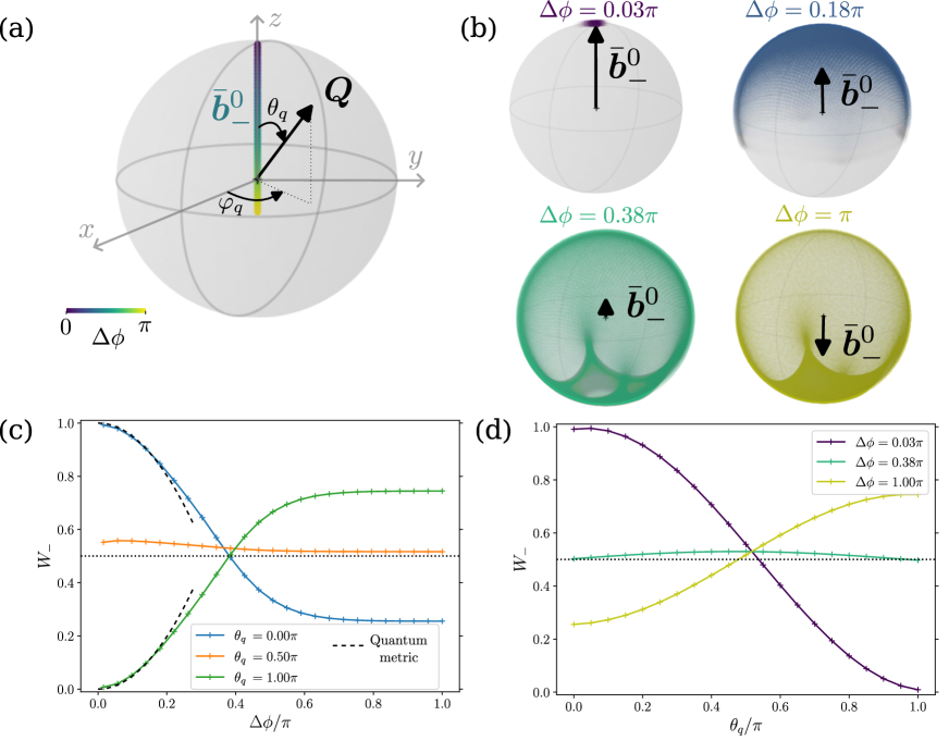
Figure 3: Weight $W_{-}$ of the adiabatic states superposition. The modes are in a Gaussian state centered on $\phi_{1}^{0}=\phi_{2}^{0}=0$. We vary the width $\Delta\phi$ of the Gaussian state and the qubit initial state $\ket{\psi_{q}}$ represented by its polarization $\bm{Q}$ on the Bloch sphere. (a) Averaged ground state $\bar{\bm{b}}_{-}^{0}$, lying on the $z$-axis. The average adiabatic state $\bar{\bm{b}}_{-}$ is pertubatively close to $\bar{\bm{b}}_{-}^{0}$. (b) The phase density $|\chi(\bm{\Phi})|^{2}$ on the torus translates via the map $\bm{\Phi}\mapsto\bm{b}_{-}(\bm{\Phi})$ to a density of adiabatic states on the Bloch sphere represented in color for different $\Delta\phi$. $\overline{\bm{b}}_{-}$ is the average of this density. (c) Weight of the cat depending on the width in phase $\Delta\phi$. The average Bloch vector remains approximately on the z-axis, such that a cat with $W_{-}=\frac{1}{2}$ is obtained for the qubit on the equator $\theta_{q}=\pi/2$. The deviation from $W_{-}=1/2$ at $\theta_{q}=\pi/2$ is due to the difference between the eigenstates and the adiabatic states. In the limit of small $\Delta\phi$ for $\ket{\psi_{q}}=\ket{\psi_{-}(\bm{\Phi}^{0})}$ ($\theta_{q}=0$) and $\ket{\psi_{q}}=\ket{\psi_{+}(\bm{\Phi}^{0})}$ ($\theta_{q}=\pi$) the weight of adiabaticity is controlled by the quantum metric $g_{-,ij}(\bm{\Phi}^{0})$ of the adiabatic states. (d) Weight of the cat depending on the initial state of the qubit, varying $\theta_{q}$ at $\varphi_{q}=0$. The norm of the average adiabatic state defines the bounds $(1\pm|\bar{\bm{b}}_{-}|)/2$ of the weight. For $\Delta\phi=0.38\pi$, $|\bar{\bm{b}}_{\pm}|\simeq 0$ such that a cat with almost equal weight is created independently of the initial state of the qubit.

II.3 Weight of the adiabatic cat state

In this section, we focus on the weight $W_{\nu}(\Psi)$ (15) of each component of the cat state. This will allow us to identify the conditions on the initial states to realize ideal adiabatic cat states with equal weights $W_{+}(\Psi)=W_{-}(\Psi)$.

We can represent the states $\ket{\psi_{\nu}(\bm{\Phi})}$ and $\ket{\psi_{q}}$ by vectors on the Bloch sphere, respectively $\bm{b}_{\nu}(\bm{\Phi})$ and $\bm{Q}$, see Fig. 3(a). The qubit’s state representation $\bm{Q}$ is parametrized by the angle $\theta_{q}$ with the $z$-axis and its azimuthal angle $\varphi_{q}$. In this section, we focus without loss of generality on $\varphi_{q}=0$, i.e. on $\bm{Q}$ lying in the $xz$ plane, and on the mode prepared in a Gaussian state centered on $\phi_{1}^{0}=\phi_{2}^{0}=0$. The adiabatic states are obtained in a perturbative expansion around the eigenstates $\ket{\psi^{0}_{\nu}(\bm{\Phi})}$. Hence they are represented by $\bm{b}_{\nu}(\bm{\Phi})$ which is perturbatively close to $\bm{b}_{\nu}^{0}(\bm{\Phi})$.

II.3.1 General expression of the weights

The phase states in the decomposition (12) being orthogonal, the weight $W_{\nu}(\Psi)$, $\nu=\pm$ is the weight of the wave amplitude $\chi_{\nu}(\bm{\Phi})=\chi(\bm{\Phi})\innerproduct{\psi_{\nu}(\bm{\Phi})}{\psi_{q}}$:

$$W_{\nu}(\Psi)=\int\differential^{2}\bm{\Phi}~{}|\chi_{\nu}(\bm{\Phi})|^{2}.$$ (19)

The overlap between $\ket{\psi_{\nu}(\bm{\Phi})}$ and $\ket{\psi_{q}}$ is $|\innerproduct{\psi_{\nu}(\bm{\Phi})}{\psi_{q}}|^{2}=(1+\bm{b}_{\nu}(\bm{\Phi})\cdot\bm{Q})/2$ such that the weight (19) now reads

$$W_{\nu}(\Psi)=\frac{1}{2}\left(1+\overline{\bm{b}}_{\nu}\cdot\bm{Q}\right)\ ,\ \nu=\pm,$$ (20)

with

$$\overline{\bm{b}}_{\nu}=\int\differential^{2}\bm{\Phi}~{}|\chi(\bm{\Phi})|^{2}~{}\bm{b}_{\nu}(\bm{\Phi})$$ (21)

the statistical average of the adiabatic states with respect to the initial phase distribution $|\chi(\bm{\Phi})|^{2}$. The phase density $|\chi(\bm{\Phi})|^{2}$ on the torus translates via the map $\bm{\Phi}\mapsto\bm{b}_{\nu}(\bm{\Phi})$ to a density of adiabatic states on the Bloch sphere. $\overline{\bm{b}}_{\nu}$ is the average of this density. We represent the density associated to the ground state $\bm{b}_{-}^{0}(\bm{\Phi})$ in colored density plot on Fig. 3(b) as well as the average ground state $\bar{\bm{b}}_{-}^{0}$ for four widths $\Delta\phi=\Delta\phi_{1}=\Delta\phi_{2}$. $\bar{\bm{b}}_{-}$ is perturbatively close to $\bar{\bm{b}}_{-}^{0}$.

For small $\Delta\phi$, the phase density is localized around $\bm{\Phi}^{0}$ and $\bar{\bm{b}}_{\nu}\approx\bm{b}_{\nu}(\bm{\Phi}^{0})$ close to the surface of the Bloch sphere. When increasing the width $\Delta\phi$, we average vectors over an increasing support on the Bloch sphere, reducing the norm $|\bar{\bm{b}}_{\pm}|$ which controls the minimum weight of the cat (Fig. 3(d)). For the chosen value $\phi_{1}^{0}=\phi_{2}^{0}=0$, $\bar{\bm{b}}_{-}^{0}$ lies on the $z$-axis as inferred from (2). In the extreme case of $\Delta\phi=\pi$ (Fock state), the density is homogeneous on the torus. However, while $\bm{b}_{\pm}(\bm{\Phi})$ covers the whole sphere, the associated density is not homogeneous due to the anisotropy of the couplings (2). This leads to a non vanishing $\bar{\bm{b}}_{-}$.

II.3.2 Symmetric cat states

Following the analysis above, we can identify two types of initial states that give rise to symmetric cat states with $W_{+}=W_{-}=\frac{1}{2}$. The first class is obtained by preparing the qubit orthogonally to this average adiabatic state $\bar{\bm{b}}_{\pm}$. For our initial phase $\bm{\Phi}^{0}$, this average adiabatic state is perturbatively closed to the $z$-axis as discussed above. Hence a qubit prepared on the equator of the Bloch sphere corresponds to two almost equal weights for all $\Delta\phi$. This corresponds to the choice made for Fig. 2. This case is represented by the orange curve on Fig. 3(c). The adiabatic weight is computed numerically from the topological splitting of the adiabatic components discussed in the previous section. The deviation to $W_{-}=1/2$ originates from the difference between the eigenstates and the adiabatic states, see appendix G for details. The second class of symmetric cat states is obtained for well chosen gaussian states of the modes: the weight (20) of the cat is bounded by $(1+|\bar{\bm{b}}_{\pm}|)/2$. For $\Delta\phi=0.38\pi$, $\bar{\bm{b}}_{\pm}\simeq 0$ such that the cat has (almost equal) weights $W_{+}=W_{-}$ independently of the initial state of the qubit $\theta_{q}$ (Fig. 3(d) green curve).

II.3.3 Quasi phase states

The only separable states lying in an adiabatic subspace, corresponding to $W_{+}=1$ or $W_{-}=1$, are pure phase states $\ket{\bm{\Phi}^{0}}\otimes\ket{\psi_{\pm}(\bm{\Phi}^{0})}$ for which $|\overline{\bm{b}}_{\pm}|=1$, shown as the blue and green curves of Fig. 3(c) in limit $\Delta\phi=0$. Given that these states are fully delocalized in quanta number $\bm{N}$, and thus in energy according to (1), we expect them to be hard to realize. Any other separable state lies at a finite distance from each adiabatic subspace and will be split into a cat state under time evolution. Let us comment on this adiabatic decomposition for almost pure phase states with small $\Delta\phi$. In this case, the correction to adiabaticity is controlled by the quantum metric $g_{\pm,ij}$ of the adiabatic states [50, 33]:

$$g_{\pm,ij}=\operatorname{Re}\bra{\partial_{\phi_{i}}\psi_{\pm}}\left(1-\ket{\psi_{\pm}}\bra{\psi_{\pm}}\right)\ket{\partial_{\phi_{j}}\psi_{\pm}}.$$ (22)

Indeed, the weight (19) is dominated by the local variations of the adiabatic states $\ket{\psi_{\pm}(\bm{\Phi})}$ over the narrow phase support $|\chi(\bm{\Phi})|^{2}$. These variations are encoded by the quantum metric: $|\innerproduct{\psi_{\pm}(\bm{\Phi}^{0}+\delta\bm{\Phi})}{\psi_{\pm}(\bm{\Phi}^{0})}|^{2}=1-\sum_{i,j}g_{\pm,ij}(\bm{\Phi}^{0})\delta\phi_{i}\delta\phi_{j}+\mathcal{O}(\delta\phi^{3})$. In the limit of a small width $(\Delta\phi_{1},\Delta\phi_{2})$ the weight (19) for $\ket{\psi_{q}}=\ket{\psi_{\pm}(\bm{\Phi}^{0})}$ reduces to

$$W_{\pm}(\Psi)=1-(\Delta\phi_{1})^{2}g_{\pm,11}(\bm{\Phi}^{0})\\ -(\Delta\phi_{2})^{2}g_{\pm,22}(\bm{\Phi}^{0})+\mathcal{O}(\Delta\phi^{4}).$$ (23)

Hence for a state close to a phase state, the first correction to $W_{\nu}$ is quadratic in $\Delta\phi=1/(2\Delta n)$ with a factor set by the quantum metric of the adiabatic states, as shown in black dashed line on Fig. 3(c).

III Characterization of cat components

Having characterized the balance between the two components of an adiabatic cat state, we now study the dynamics of each component. We will focus first on the entanglement between the qubit and the two modes, before focusing on their Bloch oscillatory dynamics in the number of quanta representation.

III.1 Entanglement

Adiabatic states naturally entangle the fast qubit with the slow driving modes, a phenomenon out-of-reach of previous Floquet or classical descriptions of the drives [14, 15, 17, 18, 19, 20, 21, 23]. We focus on cat states with almost equal weight $W_{\nu}\simeq 1/2$, obtained with $\bm{\Phi}^{0}=0$ and $\theta_{q}=\pi/2$ following the analysis of section II.3. In the following, we study the entanglement of the qubit with the modes for the different types of cat states, varying the initial spread $\Delta\phi$ of the modes and the initial azimuthal angle $\varphi_{q}$ of the qubit.

The entanglement between the qubit and the two modes in an adiabatic component $\ket{\Psi_{\nu}(t)}$, $\nu=\pm$, is captured by the purity $\gamma_{\nu}(t)=\Tr(\rho_{q,\nu}^{2}(t))=(1+|\bm{Q}_{\nu}(t)|^{2})/2$ of the qubit, where $\rho_{q,\nu}(t)$ is the reduced density matrix of the qubit and $\bm{Q}_{\nu}(t)$ its polarization. From the adiabatic time evolution (8), we deduce the reduced density matrix $\rho_{q,\nu}(t)$ of the qubit in the adiabatic state $\ket{\Psi_{\nu}(t)}$ as

$$\rho_{q,\nu}(t) =\int\differential^{2}\bm{\Phi}~{}\frac{|\chi_{\nu}(\bm{\Phi}+\bm{\omega}t)|^{2}}{W_{\nu}}\ket{\psi_{\nu}(\bm{\Phi})}\bra{\psi_{\nu}(\bm{\Phi})}$$ (24)

$$=\frac{1}{2}(\mathbb{I}+\bm{Q}_{\nu}(t)\cdot\bm{\sigma}),$$ (25)

where the polarization of the qubit $\bm{Q}_{\nu}(t)$ reads

$$\bm{Q}_{\nu}(t)=\int\differential^{2}\bm{\Phi}~{}\frac{|\chi_{\nu}(\bm{\Phi}+\bm{\omega}t)|^{2}}{W_{\nu}}\bm{b}_{\nu}(\bm{\Phi}).$$ (26)

The qubit is in the statistical mixture of the adiabatic states $\ket{\psi_{\nu}(\bm{\Phi})}$ weighted by the translated normalized phase density $|\chi_{\nu}(\bm{\Phi}+\bm{\omega}t)|^{2}/W_{\nu}$.

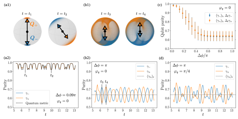
Figure 4: Purity of the qubit $\gamma_{+}(t)$ and $\gamma_{-}(t)$ in each cat components $\ket{\Psi_{+}(t)}$ and $\ket{\Psi_{-}(t)}$. The qubit is prepared on the equator $\theta_{q}=\pi/2$ to create a cat of equal weight $W_{\pm}=1/2$ for all values of $\Delta\phi$ and $\varphi_{q}$. (a1), (b1) The phase densities $|\chi_{-}(\bm{\Phi}+\bm{\omega}t)|^{2}$ and $|\chi_{+}(\bm{\Phi}+\bm{\omega}t)|^{2}$ of each cat components translates to densities of adiabatic states on the Bloch sphere (respectively in blue and orange). The qubit state is the statistical mixture weighted according to these densities with resulting polarizations $\bm{Q}_{\pm}$. (a2) For small $\Delta\phi$, the phase densities are localized around $\bm{\Phi}^{0}-\bm{\omega}t$. The adiabatic states have small variations around $\bm{\Phi}^{0}-\bm{\omega}t_{1}$ and larger variation around $\bm{\Phi}^{0}-\bm{\omega}t_{2}$, inducing $\gamma_{-}(t_{1})>\gamma_{-}(t_{2})$. These local variations are quantified by the quantum metric of the adiabatic states. (b2) (d) For large $\Delta\phi$, the adiabatic states cover a large part of the Bloch sphere, corresponding to a high entanglement. The phase densities of the two components have complementary support on the torus, leading to different densities on the Bloch sphere. The purity of each component oscillates in opposite phase around their temporal average (black dotted line). The details of the oscillations depend on the shape of the phase densities which changes with the qubit initial state $\varphi_{q}$. (c) Time average of the purity and temporal fluctuations (errorbars) depending on $\Delta\phi$. A large support $\Delta\phi$ on the torus translates to a large support on the Bloch sphere due to the topological nature of the coupling, and thus a large entanglement.

III.1.1 Entanglement of quasi-phase states.

Let us first focus on the adiabatic component of a cat obtained from a quasi-phase state of small $\Delta\phi$. We show below that entanglement between the qubit and the quantum modes of such a state is set by the quantum metric of the adiabatic states.

The translated phase density $|\chi(\bm{\Phi}+\bm{\omega}t)|^{2}$ of the modes is a normalized $2\pi$-periodic Gaussian centered on $\bm{\Phi}^{0}-\bm{\omega}t$ and of width $(\Delta\phi_{1},\Delta\phi_{2})$. Plugging expansions of Eqs. (13) and (19), and $\bm{b}_{\nu}(\bm{\Phi})$ around $\bm{\Phi}^{0}-\bm{\omega}t$ in the limit of small $\Delta\phi_{1},\Delta\phi_{2}$ into Eq. (26) we get

$$\bm{Q}_{\nu}(t)=\bm{b}_{\nu}(\bm{\Phi}^{0}-\bm{\omega}t)\\ +\frac{1}{2}\sum_{i}(\Delta\phi_{i})^{2}\frac{\partial^{2}\bm{b}_{\nu}}{\partial\phi_{i}^{2}}(\bm{\Phi}^{0}-\bm{\omega}t)+\mathcal{O}(\Delta\phi^{4}).$$ (27)

Note that in the limit $\Delta\phi_{1}=\Delta\phi_{2}=0$ of the classical description of the phase, we recover that the qubit follows the instantaneous adiabatic state $\bm{b}_{\nu}(\bm{\Phi}^{0}-\bm{\omega}t)$. From the normalization of the adiabatic states $|\bm{b}_{\nu}|^{2}=1$, we deduce the relation $\bm{b}_{\nu}\cdot\partial^{2}_{\phi_{i}}\bm{b}_{\nu}=-\partial_{\phi_{i}}\bm{b}_{\nu}\cdot\partial_{\phi_{i}}\bm{b}_{\nu}=-4g_{\nu,ii}$ where the last equation is an expression of the quantum metric of a two-level system in term of the Bloch vectors [51, 52]. From this we obtain the development at order $\Delta\phi^{2}$ of the purity

$$\gamma_{\nu}(t)=1 -2(\Delta\phi_{1})^{2}g_{\nu,11}(\bm{\Phi}^{0}-\bm{\omega}t)$$

$$-2(\Delta\phi_{2})^{2}g_{\nu,22}(\bm{\Phi}^{0}-\bm{\omega}t)+\mathcal{O}(\Delta\phi^{4}).$$ (28)

For a two level system, the quantum metric of the two levels identifies $g_{+,ij}=g_{-,ij}$ such that the qubit is equally entangled with the modes in each adiabatic component $\ket{\Psi_{\pm}}$. The topological coupling corresponds to a non-vanishing average Berry curvature $F_{\nu}$. From the inequality $g_{\nu,11}+g_{\nu,22}\geq|F_{\nu}|$ originating from the positive semidefiniteness of the quantum geometric tensor [53] we obtain a lower bound on the entanglement between the qubit and the modes:

$$\left<\gamma_{\nu}\right>_{t}\leq 1-\frac{|{\mathcal{C}}_{-}|}{\pi}(\Delta\phi)^{2}+\mathcal{O}(\Delta\phi^{4}).$$ (29)

This demonstrates that a topological pump necessarily entangles the qubit with the modes, a property only captured by the quantum description provided in this paper.

The statistical average of the adiabatic states is represented on Fig. 4(a1) for an initial width of the Gaussian state $\Delta\phi=\Delta\phi_{1}=\Delta\phi_{2}\simeq 0.09\pi$, corresponding to $\Delta n_{1}=\Delta n_{2}\simeq 2.6$, with the qubit initialized in $\varphi_{q}=0$. At a given time $t$, the densities on the torus of each component $|\chi_{\pm}(\bm{\Phi}+\bm{\omega}t)|^{2}/W_{\nu}$ is centered on $\bm{\Phi}^{0}-\bm{\omega}t$ with the initial width $\Delta\phi$. This translates into complementary densities of adiabatic states on the Bloch sphere (in blue and orange) encoding the statistical mixture of the qubit in $\ket{\Psi_{\pm}}$. In Fig. 4(a2), the purity of the qubit after the time of separation $t_{\rm sep}$ is represented respectively in blue and orange for each component $\ket{\Psi_{\pm}(t)}$. The temporal fluctuations of this purity follow those of the quantum metric at  $\bm{\Phi}^{0}-\bm{\omega}t$ represented by a black dashed line, as predicted by Eq. (28). As an illustration, we notice that the quantum metric is smaller at time $t_{1}$ than at $t_{2}$, manifesting that the evolution of adiabatic states with the phase $\bm{\Phi}$ is weaker at $\bm{\Phi}=\bm{\Phi}^{0}-\bm{\omega}t_{1}$ than at $\bm{\Phi}=\bm{\Phi}^{0}-\bm{\omega}t_{2}$. This translates into a larger purity of the qubit at $t=t_{1}$ than at $t=t_{2}$.

III.1.2 Entanglement of quasi-Fock state

We now consider states with an increasing initial width in phase $\Delta\phi$. The dependance on $\Delta\phi$ of the average in time of the of the qubit’s purity $\langle\gamma_{\pm}\rangle_{t}$ is represented on Fig. 4(c) for each adiabatic component. The amplitude of its temporal fluctuations are represented as errorbars. This average purity decreases with $\Delta\phi$, corresponding to an increase of entanglement: the larger the phase support on the torus, the larger the support on the Bloch sphere, and thus the smaller the polarization (26). The large support on the Bloch sphere originates from the topological nature of the coupling, which imposes that the adiabatic states $\bm{b}_{\pm}(\bm{\Phi})$ reaches all points of the Bloch sphere as $\bm{\Phi}$ varies. A topologically trivial coupling would lead to a localized distribution of adiabatic states on the Bloch sphere corresponding to an almost pure state of the qubit. This is another manifestation that topological pumping and entanglement between the qubit and the modes are strongly intertwined.

The time average of the purity is the same for the two adiabatic components $\langle\gamma_{+}\rangle_{t}=\langle\gamma_{-}\rangle_{t}$ for every $\Delta\phi$. A qualitative explanation is the following. Given (26) the purity $\langle\gamma_{\pm}\rangle_{t}$ corresponds to an average of adiabatic states with respect to translated phase distributions. The average over time depends only on the extension of the phase density $|\chi_{\pm}(\bm{\Phi})|^{2}$, which, from (13), satisfies

$$|\chi_{+}(\bm{\Phi}+\bm{\omega}t)|^{2}+|\chi_{-}(\bm{\Phi}+\bm{\omega}t)|^{2}=|\chi(\bm{\Phi}+\bm{\omega}t)|^{2}.$$ (30)

Hence they split the phase density of the total system $|\chi(\bm{\Phi}+\bm{\omega}t)|^{2}$ in two complementary supports, as illustrated in appendix H. For cat states with equal weight $W_{+}=W_{-}$, according to (19) these two supports have equal weight, leading to the same average purity over time.

As discussed above, for quasi phase states the purity of both components fluctuate temporally in phase Fig. 4(a2). In the opposite limit of an initial Fock state fully delocalized in phase with $\Delta\phi=\pi$, these two purities are in opposite phase. This is represented Fig. 4(b2) and (d), where the qubit is initialized respectively on $\varphi_{q}=0$ and $\varphi_{q}=\pi/4$. The phase density of the modes is uniform $|\chi(\bm{\Phi})|^{2}=1/(2\pi)^{2}$, such that according to (30) the phase density of the two cat components have complementary supports on all the torus $[0,2\pi]^{2}$. We represent on Fig 4(b1) in blue the density of adiabatic states $\bm{b}_{-}(\bm{\Phi})$ associated to the support $|\chi_{-}(\bm{\Phi}-\bm{\omega}t)|^{2}$ and in orange the density of adiabatic states $\bm{b}_{+}(\bm{\Phi})$ associated to the support $|\chi_{+}(\bm{\Phi}-\bm{\omega}t)|^{2}$. At $t=t_{3}$, the density $|\chi_{+}(\bm{\Phi}-\bm{\omega}t_{3})|^{2}$ covers a larger portion of the sphere than the density $|\chi_{-}(\bm{\Phi}-\bm{\omega}t_{3})|^{2}$, corresponding to $|\bm{Q}_{+}(t_{3})|^{2}<|\bm{Q}_{-}(t_{3})|^{2}$ and $\gamma_{+}(t_{3})<\gamma_{-}(t_{3})$ on Fig. 4(b2), while the situation is opposite at $t=t_{4}$. The details of the temporal variations of the purity depends on the details of the shape of the densities $|\chi_{\pm}(\bm{\Phi})|^{2}$, which depends on the initial state $\varphi_{q}$ of the qubit. Temporal oscillations for $\varphi_{q}=\pi/4$ are represented on Fig 4(d): the temporal average remains of the same order of magnitude and the temporal fluctuations of the purity of each components remains in opposite phase.

III.2 Breathing dynamics and Bloch oscillations

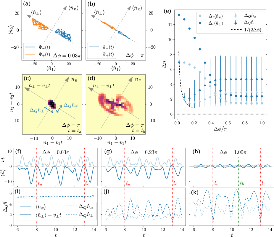
Figure 5: From Bloch oscillations to Bloch breathing. (a) Trajectories of the average values of number of quanta of each cat component $\ket{\Psi_{\pm}(t)}$ for the example of Fig. 2(a) localized in phase. The two components splits along $n_{\perp}$ at an average velocity $\pm\bm{v}=\mp(-\omega_{2},\omega_{1}){\mathcal{C}}/(2\pi)$. The Bloch oscillations are the temporal fluctuations of the average number of quanta around this drift. (b) Trajectories for the initial Fock state of Fig. 2(c). The temporal fluctuations are reduced. (c) Photon number distribution of Fig. 2(c4) zoomed on the component $\ket{\Psi_{-}(t)}$ for $t=t_{a}$ a quasi-period. (d) Photon number distribution of Fig. 2(c5) zoomed on the component $\ket{\Psi_{-}(t)}$ for $t=t_{b}$ a time of expansion. (e) Circles: amplitude $\Delta_{t}\langle\hat{n}_{\scriptscriptstyle E}\rangle$ and $\Delta_{t}\langle\hat{n}_{\perp}\rangle$ of the Bloch oscillations depending on the width in phase $\Delta\phi$. Triangle: temporal average of the spreading $\Delta_{Q}\hat{n}_{\scriptscriptstyle E}$ and $\Delta_{Q}\hat{n}_{\perp}$, with the amplitude of their temporal fluctuations in errorbar. In small $\Delta\phi$ limit, the spreading is constant, the state remains gaussian with $\Delta_{Q}\hat{n}_{i}=1/(2\Delta\phi)$. When $\Delta\phi$ increases, the amplitude of the Bloch oscillations $\Delta_{t}\langle\hat{n}_{i}\rangle$ decreases and the temporal fluctuations of the spreading increase, corresponding to a breathing. (f,g,h) Bloch oscillations. Temporal fluctuations of the average value of number of quanta $\langle\bm{\hat{N}}\rangle$ in the component $\ket{\Psi_{-}(t)}$ around the quantized drift $\bm{v}t$. At quasi-periods $t=t_{a}$ and $t=t_{b}$, the evolution is almost given by the quantized drift $\langle\bm{\hat{N}}\rangle=vt$. The increase of $\Delta\phi$ corresponds to a decrease of the temporal fluctuations. (i) Time evolution of the spreading $\Delta_{Q}\hat{n}_{i}$ in the component $\ket{\Psi_{-}(t)}$ for an initial state localized in phase. The state remains Gaussian with constant spreading $\Delta_{Q}\hat{n}_{i}=1/(2\Delta\phi)$. (j,k) Bloch breathing of the spreading for small $\Delta\phi$. The wavepacket localizes at quasi-periods $t=t_{a}$ and $t=t_{c}$, and expand in between ($t=t_{b}$).

We now discuss in more details the oscillations of both the center of mass and of the width in number of each adiabatic component of cat states that manifest themselves on the examples of Fig. 2. This dynamics is reminiscent of Bloch oscillations and Bloch breathing [54, 55, 56, 24]. Bloch oscillations correspond to temporal oscillations of the center of a wave-packet on a lattice when submitted to an electric field. Bloch breathing corresponds to temporal oscillations of the width of this wave-packet. The nature of these oscillations and breathing depends on the width of the wavepacket’s momentum distribution. In our context, the lattice correspond to the numbers of quanta $\bm{N}=(n_{1},n_{2})$ of mode. The first term of the Hamiltonian (1) is linear in $\bm{N}$ and plays the role of the coupling to an electric field $\bm{\omega}$, while the second term correspond to a spin-orbit coupling as discussed in section I.1. Hence the dynamics in $\bm{N}$ representation of the adiabatic components identifies with the Bloch oscillations and breathing in the presence of both a longitudinal electric field and an anomalous transverse topological velocity.

III.2.1 Qualitative evolution of an adiabatic component

Two trajectories of the average value of number of quanta $\langle\hat{\bm{N}}\rangle_{\Psi_{\pm}(t)}$ are represented on Fig. 5(a) and (b) for two widths $\Delta\phi$. The two adiabatic subspaces $\nu=\pm$ are associated to opposite anomalous velocities $\mp\bm{v}$ with $\bm{v}=(\omega_{2},-\omega_{1}){\mathcal{C}}_{-}/(2\pi)$. This induces a drift of the two wavepackets in opposite directions along $n_{\perp}$, shown on the figure. We highlight the dynamics of the component $\ket{\Psi_{-}(t)}$ around this drift on Fig. 5(c) and (d), the results for $\ket{\Psi_{+}(t)}$ being similar. In this figure, we note $\langle\hat{n}_{i}\rangle(t)$ the average values of $\hat{n}_{i}$ in $\ket{\Psi_{-}(t)}$ in the rotated coordinates (5), $\hat{n}_{i}$ referring to $\hat{n}_{\scriptscriptstyle E}$ or $\hat{n}_{\perp}$. We denote as $\Delta_{Q}\hat{n}_{i}(t)=[\langle\hat{n}_{i}^{2}\rangle(t)-\langle\hat{n}_{i}\rangle(t)^{2}]^{\frac{1}{2}}$ the quantum fluctuations, or spreading of $\hat{n}_{i}$ in $\ket{\Psi_{-}(t)}$ Fig. 5(c-d).

The numbers of quanta $\langle\hat{\bm{N}}\rangle(t)$ have temporal fluctuations around the quantized drift $\bm{v}t$ represented on Fig. 5(f-h) for the three adiabatic cats of Fig. 2. When we increase the width $\Delta\phi$ of the initial state, the amplitude $\Delta_{t}\langle\hat{n}_{i}\rangle$ of these temporal fluctuations is reduced, while the spreading of the wavepacket $\Delta_{Q}\hat{n}_{i}$ increases. For small $\Delta\phi$, $\Delta_{Q}\hat{n}_{i}$ is almost constant (Fig. 5(i)), the state remains Gaussian with its initial width $\Delta_{Q}\hat{n}_{i}=1/(2\Delta\phi)$ as illustrated on Fig. 2(a1-a4). When $\Delta\phi$ increases, $\Delta_{Q}\hat{n}_{i}$ oscillates in time 5(j-k). This corresponds to breathing: oscillations, such as at $t=t_{b}$ on Fig. 5(d), between relocalization occurring e.g. at $t=t_{a}$ and $t_{c}$ on Fig. 5(c). The corresponding time evolution of the width $\Delta_{Q}\hat{n}_{i}$ is represented on Fig. 5(i-k).

III.2.2 Quasi-periods

In Fig. 5(j-k), we observe, for a large initial $\Delta\phi$, a relocalization of the wavepacket at specific times such as $t_{a}$ and $t_{c}$. These fluctuations in time of the adiabatic wave-packet correspond to two dimensional Bloch oscillations  [54, 55, 56]. Historically, Bloch oscillations were first considered in one dimension [57]. The electric field induces a constant increase of the Bloch momenta of a semiclassical wavepacket, which crosses periodically the one dimensional Brillouin zone. As a consequence the average position of the wavepacket oscillates periodically. In two dimensions, Bloch oscillations are richer. The Bloch momenta evolves on the two dimensional Brillouin zone along the direction of the electric field: $\bm{\Phi}(t)=\bm{\Phi}^{0}-\bm{\omega}t$. Such an evolution is periodic for a commensurate ratio between $\omega_{1}$ and $\omega_{2}$, corresponding to an electric field in a crystalline direction. Noting $\omega_{1}/\omega_{2}=p_{1}/p_{2}$ with $p_{1}$ and $p_{2}$ coprime integers, the trajectory of the Bloch momenta on the two dimensional Brillouin zone is periodic with period $T=p_{1}2\pi/\omega_{1}=p_{2}2\pi/\omega_{2}$. In practice any real number $\omega_{1}/\omega_{2}$ can be approximated by a set of rational numbers [55, 24]. Each rational approximation leads to a quasi period $T$ for which $\bm{\Phi}^{0}-\bm{\omega}T\simeq\bm{\Phi}^{0}$. The times $t_{a}$ and $t_{c}$ on Fig. 5 are two examples of these quasi-periods for our choice of $\omega_{1},\omega_{2}$.

The periodicity of a trajectory on the Brillouin zone translates into a periodic motion in the direction of the electric field $n_{\scriptscriptstyle E}$ but not in the transverse direction $n_{\perp}$, even in the absence of an anomalous velocity [56, 58]. For an initial phase $\bm{\Phi}^{0}$, the classical equations of motion in adiabatic space $\nu$ of the center of the wavepacket can be written as [14, 23]:

$$n_{\scriptscriptstyle E}(t) =\int_{0}^{t}\frac{1}{\hbar}\frac{\partial E_{\nu}}{\partial\phi_{\scriptscriptstyle E}}(\bm{\Phi}(t^{\prime}))\differential t^{\prime}\ ,$$ (31)

$$n_{\perp}(t) =\int_{0}^{t}\left(\frac{1}{\hbar}\frac{\partial E_{\nu}}{\partial\phi_{\perp}}(\bm{\Phi}(t^{\prime}))-|\bm{\omega}|F_{\nu}(\bm{\Phi}(t^{\prime}))\right)\differential t^{\prime}.$$ (32)

where the evolution of the phase reads in the rotated phase coordinates: $\phi_{\scriptscriptstyle E}(t)=\phi_{\scriptscriptstyle E}^{0}-|\bm{\omega}|t$ and $\phi_{\perp}(t)=\phi_{\perp}^{0}$. We choose the origin of the number of quanta set by their initial values, such that $n_{\scriptscriptstyle E}(0,\bm{\Phi}^{0})=n_{\perp}(0,\bm{\Phi}^{0})=0$. The time integral can be rewritten as a line integral over $\phi_{\scriptscriptstyle E}$, leading to the conservation equation $\hbar|\bm{\omega}|n_{\scriptscriptstyle E}(t,\bm{\Phi}^{0})=E_{\nu}(\bm{\Phi}^{0})-E_{\nu}(\bm{\Phi}(t))$, which is vanishingly small at a quasi-period $T$ such that $\bm{\Phi}(T)\simeq\bm{\Phi}^{0}$. A quasi-period defines an almost closed trajectory on the torus. The line integral of (32) does not vanish on this closed trajectory, and reads $n_{\perp}(T,\bm{\Phi}^{0})\simeq vT$. The approximation gets better for longer quasi-periods $T$, i.e. large $p_{1}$ and $p_{2}$.

III.2.3 Bloch oscillations of the average number of quanta

In the hybrid classical-quantum description of a topological pump [14, 23], the topological quantization of the pumping rate is recovered under a time-average of the instantaneous flux of quanta $\dot{n}_{i}(t)$. This time average of the Berry curvature entering the pumping rate is set by the Chern number of the adiabatic states over the torus $[0,2\pi]^{2}$. The quantum nature of the mode induces another source of averaging. The time evolution of the average number of quanta (16) corresponds to an average of the classical evolution (32) with respect to the phase density $|\chi_{\nu}(\bm{\Phi})|^{2}$ of the adiabatic component. Thus an increase of the support $|\chi_{\nu}(\bm{\Phi})|^{2}$ reduces the temporal fluctuations of the average number of quanta around its average drift. The quantization of topological pumping is indeed better between quantum than classical modes. This is represented on Fig. 5(e). We note $\Delta_{t}\langle\hat{n}_{i}\rangle$ the amplitude of the fluctuations with time of the average value of $\langle\hat{n}_{i}\rangle$. These temporal fluctuations are reduced when $\Delta\phi$ increases (circles on Fig. 5(e)).

The reduction of the temporal fluctuations of pumping is set by the width of the phase density $|\chi_{\nu}(\bm{\Phi})|^{2}$. One would expect that a complete delocalization in phase, $|\chi_{\nu}(\bm{\Phi})|^{2}=1/(2\pi)^{2}$, averages instantaneously the classical pumping rate over the whole phase space such that $\langle\hat{\bm{N}}\rangle(t)\simeq\bm{v}t$ without any temporal fluctuations. Such a projected state with uniform delocalization in $\bm{\Phi}$ corresponds to a Wannier state for a particle on a lattice which is topologically obstructed [59, 60, 61]. First, let us note that the spreading $\Delta_{Q}\hat{n}_{i}$ is infinite in such obstructed Wannier state, making them hard to realize experimentally. Moreover, due to the adiabatic decomposition (11) of the initial (separable) state, such adiabatic states are never realized: the phase density $|\chi_{\nu}(\bm{\Phi})|^{2}$, defined in (13) contains the density of projection of the qubit initial state $|\innerproduct{\psi_{\nu}(\bm{\Phi})}{\psi_{q}}|^{2}$ which necessarily vanishes on the configuration space for a topological pump, irrespective of $\ket{\psi_{q}}$. A Wannier state cannot be obtained by the adiabatic decomposition of a separable state, and the temporal fluctuations of the pumping remain finite.

III.2.4 Bloch breathing of the spreading

When the phase density $|\chi_{\nu}(\bm{\Phi})|^{2}$ is localized around $\bm{\Phi}^{0}$, the center of mass performs Bloch oscillations following the classical trajectory $\bm{N}(t,\bm{\Phi}^{0})$ (31), (32). Intuitively, when the adiabatic state has a large support in phase $|\chi_{\nu}(\bm{\Phi})|^{2}$, the different trajectories $\bm{N}(t,\bm{\Phi})$ on this support superpose, inducing a spreading of the wavepacket. The spreading of the wavepacket is then captured by the variance $\text{Var}_{|\chi_{\nu}|^{2}}[n_{i}(t,\bm{\Phi})]$ of the classical trajectories with respect to the (normalized) initial phase distribution $|\chi_{\nu}(\bm{\Phi})|^{2}/W_{\nu}$:

$$\text{Var}_{|\chi_{\nu}|^{2}}[n_{i}(t,\bm{\Phi})]=\int\differential^{2}\bm{\Phi}~{}\frac{|\chi_{\nu}(\bm{\Phi})|^{2}}{W_{\nu}}n_{i}(t,\bm{\Phi})^{2}\ \\ -\left(\int\differential^{2}\bm{\Phi}~{}\frac{|\chi_{\nu}(\bm{\Phi})|^{2}}{W_{\nu}}n_{i}(t,\bm{\Phi})\right)^{2}.$$ (33)

We show in appendix I that the time evolution of the spreading $\Delta_{Q}\hat{n}_{i}$ in the adiabatic state $\ket{\Psi_{\nu}(t)}$ is indeed related to this variance, and is the sum of three different terms.

For a quasi-phase state with a narrow distribution $|\chi_{\nu}(\bm{\Phi})|^{2}$, the classical trajectories for an initial phase on this support are all similar, such that the variance term (33) vanishes. The quantum fluctuations weakly evolve in time $\Delta_{Q}\hat{n}_{i}(t)\simeq\Delta_{Q}\hat{n}_{i}(0)\simeq 1/(2\Delta\phi)$, as shown in Fig. 5(i). In the case of large $\Delta\phi$, the classical evolution $n_{i}(t,\bm{\Phi})$ follows different trajectories for the different values of $\bm{\Phi}$ on $|\chi_{\nu}(\bm{\Phi})|^{2}$, leading to a large $\text{Var}_{|\chi_{\nu}|^{2}}[n_{i}(t,\bm{\Phi})]$ and an expansion of the wavepacket, seen for example at $t=t_{b}$ on Fig. 5(d)(k). At a quasi-period $T$ discussed in Sec. III.2.2, the classical trajectories leads almost to the same quantized drift $\bm{N}(T,\bm{\Phi})\simeq\bm{v}T$ for all initial phases $\bm{\Phi}$, such that $\text{Var}_{|\chi_{\nu}|^{2}}[n_{i}(T,\bm{\Phi})]\simeq 0$. The wave-packet refocuses at these quasi-periods, seen at $t=t_{a}$ and $t=t_{c}$ on Fig. 5(k).

The default of refocusing is usually discussed in the literature in relation with the default of rephasing $\text{Var}_{|\chi_{\nu}|^{2}}[n_{i}(T,\bm{\Phi})]\neq 0$ [24, 54], such that $(\Delta_{Q}\hat{n}_{i})(T)\gtrsim(\Delta_{Q}\hat{n}_{i})(t=0)$. We note an important point about these rephasing: even if the refocusing is perfect $(\Delta_{Q}\hat{n}_{i})(T)=(\Delta_{Q}\hat{n}_{i})(t=0)$ the spread at these refocusing times corresponds to the initial spread of the adiabatic component $\ket{\Psi_{-}(t=0)}$ and not to the initial state $\ket{\Psi(t=0)}$. This is the reason why on Fig. 5(c) the state does not refocus into a Fock state. Indeed, as discussed above the phase distribution $|\chi_{-}(\bm{\Phi})|^{2}$ is not fully delocalized on the torus, such that by Heisenberg inequality the distribution of number of quanta in $\ket{\Psi_{-}(t=0)}$ is not fully localized. For the cat state with equal weight, we discussed in section III.1 that $|\chi_{-}(\bm{\Phi})|^{2}$ cover approximately half the torus, corresponding to a spread of order $\pi/4$, such that $\Delta_{Q}\hat{n}_{i}(t=0)\geq 2/\pi\simeq 0.63$. This is approximately the values of the spreading at the refocusing times on Fig. 5(k).

IV Discussion

In this work, we have shown that the dynamics of a qubit coupled topologically to two slow quantum modes generically creates a cat state, a superposition of two adiabatic states with mesoscopically distinct energy content. For each adiabatic component of the cat, the topological nature of the coupling induces an intrinsic entanglement between the qubit and the modes.

The realization of such topological adiabatic cat states opens interesting perspectives, in particular to elaborate protocols to disentangle the qubit from the quantum modes, creating an entangled cat state between the modes. One can build on existing protocols for a superconducting qubit dispersively coupled to quantum cavities, with cat composed of coherent states non-entangled with the qubit, of typical form $(\ket{\alpha_{1},\alpha_{2},\uparrow}+\ket{\beta_{1},\beta_{2},\downarrow})/\sqrt{2}$ [62]. From our analysis of Sec. III.1, similar states are obtained from an adiabatic cat state in the quasi-phase limit at a time $t$ where a small value of the quantum metric $g_{ij}(\bm{\Phi}^{0}-\bm{\omega}t)$ is reached. Besides, it is worth point out that the topological splitting of the two adiabatic components allows for the experimental preparation of adiabatic states, by using a projection on the number of quanta $(n_{1},n_{2})$ such that $n_{1}-n_{2}>n_{1}^{0}-n_{2}^{0}$ after the time of separation. In the perspective of a superconducting qubit coupled to quantum cavities, such a measurement protocol can be adapted from the methods of photon number resolution [63] using an additional qubit dispersively coupled to the two cavities.

Finally, let us stress that we have focused on the adiabatic limit of a quantum description of a Floquet system. We characterized the entanglement between the drives and the driven quantum system in term of the quantum geometry of adiabatic states. Extending this relation between entanglement and geometry beyond the adiabatic limit [64, 65] is a natural and stimulating perspective.

Appendix A Time evolution of phase states

We consider the Hamiltonian $\hat{H}_{\rm tot}=\hbar\bm{\omega}\cdot\hat{\bm{N}}+H(\hat{\bm{\Phi}})$ where $\bm{\omega}=(\omega_{1},\cdots,\omega_{N})$, $\hat{\bm{N}}=(\hat{n}_{1},\cdots,\hat{n}_{N})$, $\hat{\bm{\Phi}}=(\hat{\phi}_{1},\cdots,\hat{\phi}_{N})$, where the operators $\hat{n}_{i}$ and $\hat{\phi}_{i}$ are conjugated $[\hat{n}_{i},\hat{\phi}_{j}]={\rm i}\delta_{i,j}\mathbf{1}$, and $\bm{\omega}\cdot\hat{\bm{N}}=\sum_{i}\omega_{i}\hat{n}_{i}$. We determine the time evolution of a phase eigenstate $\ket{\Psi(t=0)}=\ket{\bm{\Phi}}\otimes\ket{\psi}$ with $\ket{\psi}$ is an arbitrary state of the two-level system. In the interaction representation with respect to the Hamiltonian of the modes, the time evolved state is:

$$\ket{\Psi_{I}(t)}=\exp\left[{\rm i}t\bm{\omega}\cdot\hat{\bm{N}}\right]\ket{\Psi(t)}.$$ (34)

The dynamics of $\ket{\Psi_{I}(t)}$ is governed by the Hamiltonian in the interaction representation:

$$\hat{H}_{I}(t) =\exp\left[{\rm i}t\bm{\omega}\cdot\hat{\bm{N}}\right]H(\hat{\bm{\Phi}})\exp\left[-{\rm i}t\bm{\omega}\cdot\hat{\bm{N}}\right]$$ (35)

$$=H(\hat{\bm{\Phi}}-\bm{\omega}t)$$ (36)

since the operators $\hat{n}_{i}$ are generators of the phase translation. As a consequence,

$$\hat{H}_{I}(t)\left(\ket{\bm{\Phi}}\otimes\ket{\psi}\right)=\ket{\bm{\Phi}}\otimes H(\bm{\Phi}-\bm{\omega}t)\ket{\psi}$$ (37)

such that the time-evolution of the initial state $\ket{\bm{\Phi}}\otimes\ket{\psi}$ in the interaction representation is

$$\ket{\Psi_{I}(t)} =\mathcal{T}\exp\left[-\frac{{\rm i}}{\hbar}\int_{0}^{t}\differential\tau~{}\hat{H}_{I}(\tau)\right]\ket{\bm{\Phi}}\otimes\ket{\psi}$$

$$=\ket{\bm{\Phi}}\otimes U(t;\bm{\Phi})\ket{\psi}$$ (38)

where $\mathcal{T}$ denotes time-ordering and $U(t;\bm{\Phi})=\mathcal{T}\exp\left[-\frac{{\rm i}}{\hbar}\int_{0}^{t}\differential\tau~{}H(\bm{\Phi}-\bm{\omega}\tau)\right]$ is the time evolution operator associated to the time-dependant Hamiltonian $H(\bm{\Phi}-\bm{\omega}t)$ for classical modes. We then obtain the time-evolved state in the Schrödinger representation

$$\ket{\Psi(t)} =\exp\left[-{\rm i}t\bm{\omega}\cdot\hat{\bm{N}}\right]\ket{\Psi_{I}(t)}$$ (39)

$$=\ket{\bm{\Phi}-\bm{\omega}t}\otimes U(t;\bm{\Phi})\ket{\psi}.$$ (40)

Appendix B Construction of the adiabatic subspaces

We construct the states of the two-level system $\ket{\psi_{\nu}(\bm{\Phi})}$ such that the family of states $\ket{\bm{\Phi}}\otimes\ket{\psi_{\nu}(\bm{\Phi})}$ with $\bm{\Phi}\in[0,2\pi]^{2}$ is stable under the dynamics governed by the total Hamiltonian $H_{\rm tot}=\sum_{i}\hbar\omega_{i}\hat{n}_{i}+H(\hat{\bm{\Phi}})$. This family of states corresponds to the image of the associated adiabatic projector

$$\hat{P}_{\nu} =\int\differential\bm{\Phi}~{}\ket{\bm{\Phi}}\bra{\bm{\Phi}}\otimes\ket{\psi_{\nu}(\bm{\Phi})}\bra{\psi_{\nu}(\bm{\Phi})}$$ (41)

$$=\int\differential\bm{\Phi}~{}\ket{\bm{\Phi}}\bra{\bm{\Phi}}\otimes\pi_{\nu}(\bm{\Phi}).$$ (42)

We first construct the family of projectors of the two-level system $\pi_{\nu}(\bm{\Phi})=\ket{\psi_{\nu}(\bm{\Phi})}\bra{\psi_{\nu}(\bm{\Phi})}$. As detailed in appendix A, for an arbitrary state $\ket{\psi}$ of the fast quantum degree of freedom, the phase eigenstates evolve according to

$$\exp(-i\hat{H}_{\rm tot}t/\hbar)\left(\ket{\bm{\Phi}}\otimes\ket{\psi}\right)=\ket{\bm{\Phi}-\bm{\omega}t}\otimes U(t;\bm{\Phi})\ket{\psi}$$ (43)

with $U(t;\bm{\Phi})$ the time evolution operator associated to the Floquet Hamiltonian $H(\bm{\Phi}-\bm{\omega}t)$. Thus the previous family of states is stable if the projectors $\pi_{\nu}(\bm{\Phi})$ satisfy

$$U(t;\bm{\Phi})\pi_{\nu}(\bm{\Phi})U(t;\bm{\Phi})^{\dagger}=\pi_{\nu}(\bm{\Phi}-\bm{\omega}t)\,,$$ (44)

or equivalently $-i\hbar\bm{\omega}\cdot\nabla_{\bm{\Phi}}\pi_{\nu}(\bm{\Phi})=[H(\bm{\Phi}),\pi_{\nu}(\bm{\Phi})].$ This equation can be solved perturbatively, assuming that the eigenstates evolve slowly. Similarly to [66], we rescale all of the frequencies by a dimensionless parameter $\epsilon$: $\bm{\omega}\to\epsilon\bm{\omega}$. We search a projector $\pi_{\nu}(\bm{\Phi})$ expressed a formal series of $\epsilon$

$$\pi_{\nu}(\bm{\Phi})=\sum_{k}\epsilon^{k}\pi_{\nu,k}(\bm{\Phi})=\pi_{\nu,0}(\bm{\Phi})+\epsilon\pi_{\nu,1}(\bm{\Phi})+\dots$$ (45)

solution of the equations

$$-i\epsilon\hbar\bm{\omega}\cdot\nabla_{\bm{\Phi}}\pi_{\nu}(\bm{\Phi}) =[H(\bm{\Phi}),\pi_{\nu}(\bm{\Phi})]$$ (46)

$$\pi_{\nu}(\bm{\Phi})^{2} =\pi_{\nu}(\bm{\Phi})\,.$$ (47)

Such a solution exists as an asymptotic series in $\epsilon$ [46, 47, 67].

We detail the determination of the two first terms. The conditions (46) and (47) gives for the order 0

$$[H(\bm{\Phi}),\pi_{\nu,0}(\bm{\Phi})] =0$$ (48)

$$\pi_{\nu,0}(\bm{\Phi})^{2} =\pi_{\nu,0}(\bm{\Phi})$$ (49)

which is satisfied for a family of projectors $\pi_{\nu,0}(\bm{\Phi})=\ket{\psi_{\nu}^{0}(\bm{\Phi})}\bra{\psi_{\nu}^{0}(\bm{\Phi})}$ on eigenstates $\ket{\psi_{\nu}^{0}(\bm{\Phi})}$ of $H(\bm{\Phi})$ associated to the eigen-energy $E_{\nu}^{0}(\bm{\Phi})$, $H(\bm{\Phi})\ket{\psi_{\nu}^{0}(\bm{\Phi})}=E_{\nu}^{0}(\bm{\Phi})\ket{\psi_{\nu}^{0}(\bm{\Phi})}$. At order 1, the conditions (46) and (47) read

$$[H(\bm{\Phi}),\pi_{\nu,1}(\bm{\Phi})] =i\hbar\bm{\omega}\cdot\nabla_{\bm{\Phi}}\pi_{\nu,0}(\bm{\Phi})$$ (50)

$$\pi_{\nu,1}(\bm{\Phi}) =\pi_{\nu,1}(\bm{\Phi})\pi_{\nu,0}(\bm{\Phi})+\pi_{\nu,0}(\bm{\Phi})\pi_{\nu,1}(\bm{\Phi}).$$ (51)

When the eigenstate $\ket{\psi_{\nu}^{0}(\bm{\Phi})}$ is non-degenerate for all $\bm{\Phi}\in[0,2\pi]^{2}$, these equations are satisfied for

$$\pi_{\nu,1}(\bm{\Phi})=\sum_{\mu\neq\nu}\ket{\psi_{\mu}^{0}(\bm{\Phi})}\frac{\sum_{i}\hbar\omega_{i}A_{\mu\nu,i}^{0}(\bm{\Phi})}{E_{\mu}^{0}(\bm{\Phi})-E_{\nu}^{0}(\bm{\Phi})}\bra{\psi_{\nu}^{0}(\bm{\Phi})}+\mathrm{h.c.}$$ (52)

with $A_{\mu\nu,i}^{0}(\bm{\Phi})=i\innerproduct{\psi_{\mu}^{0}(\bm{\Phi})}{\partial_{\phi_{i}}\psi_{\nu}^{0}(\bm{\Phi})}$ the components of the non-abelian Berry connection of the eigenstates. Thus the adiabatic state at order 1 decomposes on the eigenstates similarly to the usual time dependant perturbation theory

$$\ket{\psi_{\nu}(\bm{\Phi})}=\ket{\psi_{\nu}^{0}(\bm{\Phi})}+\\ \epsilon\sum_{\mu\neq\nu}\left(\frac{\sum_{i}\hbar\omega_{i}A_{\mu\nu,i}^{0}(\bm{\Phi})}{E_{\mu}^{0}(\bm{\Phi})-E_{\nu}^{0}(\bm{\Phi})}\right)\ket{\psi_{\mu}^{0}(\bm{\Phi})}+\mathcal{O}(\epsilon^{2}).$$ (53)

Appendix C Time evolution of the adiabatic states

In appendix B we constructed the projectors $\pi_{\nu}(\bm{\Phi})=\ket{\psi_{\nu}(\bm{\Phi})}\bra{\psi_{\nu}(\bm{\Phi})}$ on the states of the two-level system such that the image of the adiabatic projector $\hat{P}_{\nu}$ is stable under the dynamics. As discussed in the main text, such states $\ket{\psi_{\nu}(\bm{\Phi})}$ have to satisfy

$$U(t;\bm{\Phi})\ket{\psi_{\nu}(\bm{\Phi})}=e^{i\theta_{\nu}(t;\bm{\Phi})}\ket{\psi_{\nu}(\bm{\Phi}-\bm{\omega}t)}$$ (54)

with $U(t;\bm{\Phi})$ the time evolution operator associated to the time-dependant Hamiltonian $H(\bm{\Phi}-\bm{\omega}t)$ and with $\theta_{\nu}(t;\bm{\Phi})$ a phase factor. We show that this phase factor is related to the Aharonov-Anandan phase. By definition, the time evolution operator $U(t;\bm{\Phi})$ satisfies

$$i\hbar\frac{\differential}{\differential t}U(t;\bm{\Phi}) =H(\bm{\Phi}-\bm{\omega}t)U(t;\bm{\Phi})$$ (55)

such that (54) gives

$$\frac{1}{i\hbar}H(\bm{\Phi}-\bm{\omega}t)\ket{\psi_{\nu}(\bm{\Phi}-\bm{\omega}t)}=i\frac{\partial\theta_{\nu}}{\partial t}(t;\bm{\Phi})\ket{\psi_{\nu}(\bm{\Phi}-\bm{\omega})}\\ -\sum_{i}\omega_{i}\ket{\partial_{\phi_{i}}\psi_{\nu}(\bm{\Phi}-\bm{\omega}t)}.$$ (56)

The phase factor $\theta_{\nu}(t;\bm{\Phi})$ is then given by

$$\theta_{\nu}(t;\bm{\Phi})=\int_{0}^{t}\differential t^{\prime}\left(-\frac{1}{\hbar}E_{\nu}(\bm{\Phi}-\bm{\omega}t^{\prime})-\sum_{i}\omega_{i}A_{\nu,i}(\bm{\Phi}-\bm{\omega}t^{\prime})\right)$$ (57)

with the energy function

$$E_{\nu}(\bm{\Phi})=\bra{\psi_{\nu}(\bm{\Phi})}H(\bm{\Phi})\ket{\psi_{\nu}(\bm{\Phi})}$$ (58)

and the (generalized) Berry connection

$$A_{\nu,i}(\bm{\Phi})=i\innerproduct{\psi_{\nu}(\bm{\Phi})}{\partial_{\phi_{i}}\psi_{\nu}(\bm{\Phi})}$$ (59)

of the adiabatic states $\ket{\psi_{\nu}(\bm{\Phi})}$.

Appendix D Pumping rate in an adiabatic state

We derive the time-evolution (16) of the pumping rate $\langle\hat{n}_{1}\rangle$ for an initial state (11) projected in the adiabatic subspace $\nu$

$$\ket{\Psi_{\nu}(t=0)}=\int\differential^{2}\bm{\Phi}~{}\chi_{\nu}(\bm{\Phi})\ket{\bm{\Phi}}\otimes\ket{\psi_{\nu}(\bm{\Phi})}.$$ (60)

From appendix C, the time evolution of this projected state is

$$\ket{\Psi_{\nu}(t)}=\int\differential^{2}\bm{\Phi}~{}\chi_{\nu}(\bm{\Phi})e^{i\theta_{\nu}(t;\bm{\Phi})}\ket{\bm{\Phi}-\bm{\omega}t}\otimes\ket{\psi_{\nu}(\bm{\Phi}-\bm{\omega}t)}.$$ (61)

with the phase factor $\theta_{\nu}(t;\bm{\Phi})$ given by (57). The Ehrenfest theorem reads

$$\frac{\differential}{\differential t}\langle\hat{n}_{1}\rangle_{\Psi_{\nu}(t)}=\frac{1}{i\hbar}\langle[\hat{n}_{1},\hat{H}_{\rm tot}]\rangle_{\Psi_{\nu}(t)}$$ (62)

where from the Hamiltonian (1) we have $[\hat{n}_{1},\hat{H}_{\rm tot}]=i\frac{\partial H}{\partial\phi_{1}}(\hat{\bm{\Phi}})$ such that

$$\frac{\differential}{\differential t}\langle\hat{n}_{1}\rangle_{\Psi_{\nu}(t)}=\int\differential^{2}\bm{\Phi}~{}\frac{|\chi_{\nu}(\bm{\Phi})|^{2}}{W_{\nu}}\\ \frac{1}{\hbar}\bra{\psi_{\nu}(\bm{\Phi}-\bm{\omega}t)}\frac{\partial H}{\partial\phi_{1}}(\bm{\Phi}-\bm{\omega}t)\ket{\psi_{\nu}(\bm{\Phi}-\bm{\omega}t)}$$ (63)

with $W_{\nu}=\innerproduct{\Psi_{\nu}(t)}{\Psi_{\nu}(t)}$ given by (21). The average value of the derivative of the Hamiltonian can be written

$$\bra{\psi_{\nu}}\frac{\partial H}{\partial\phi_{1}}\ket{\psi_{\nu}}=\frac{\partial}{\partial\phi_{1}}\left(\bra{\psi_{\nu}}H\ket{\psi_{\nu}}\right)\\ -\bra{\partial_{\phi_{1}}\psi_{\nu}}H\ket{\psi_{\nu}}-\bra{\psi_{\nu}}H\ket{\partial_{\phi_{1}}\psi_{\nu}}$$ (64)

where the dependance on $\bm{\Phi}-\bm{\omega}t$ is implicit. The first term of this equation gives the term of variation of energy in (16). Using the expression (56) for $H\ket{\psi_{\nu}}$ and using the normalization condition $\innerproduct{\partial_{\phi_{1}}\psi_{\nu}}{\psi_{\nu}}=-\innerproduct{\psi_{\nu}}{\partial_{\phi_{1}}\psi_{\nu}}$, we write the last two terms of (64) in term of the curvature $F_{\nu}$ (14) such that we obtain the expression (16) of the pumping rate

$$\frac{\differential}{\differential t}\langle\hat{n}_{1}\rangle_{\Psi_{\nu}(t)}=\int\differential^{2}\bm{\Phi}~{}\frac{|\chi_{\nu}(\bm{\Phi})|^{2}}{W_{\nu}}\\ \left(\frac{1}{\hbar}\frac{\partial E_{\nu}}{\partial\phi_{1}}(\bm{\Phi}-\bm{\omega}t)+\omega_{2}F_{\nu}(\bm{\Phi}-\bm{\omega}t)\right)$$ (65)

with the energy function $E_{\nu}(\bm{\Phi})=\bra{\psi_{\nu}(\bm{\Phi})}H(\bm{\Phi})\ket{\psi_{\nu}(\bm{\Phi})}$ and the curvature $F_{\nu}$ (14). This expression identifies with the time evolution obtained within a classical-quantum description [14, 23] weighted by the normalized phase wavepacket density $|\chi_{\nu}(\bm{\Phi})|^{2}/W_{\nu}(\Psi)$ of the adiabatic component. The quantum evolution is recovered from an average of classical trajectories, this is due to the linearity in $\hat{\bm{N}}$ of the Hamiltonian such that in phase representation the evolution of the wavepacket (61) is non-dispersive.

Appendix E Gaussian phase states

The modes are prepared in a Gaussian state $\innerproduct{n_{i}}{\chi_{i}}\propto\exp(-(n_{i}-n_{i}^{0})^{2}/(2\Delta n_{i})^{2}+i\phi_{i}^{0}n_{i})$ centered on $(n_{i}^{0},\phi_{i}^{0})$, and of width $\Delta n_{i}$. In the case of a quantum harmonic oscillator for which $\hat{n}_{i}=\hat{a}^{\dagger}\hat{a}$, a coherent state $\ket{\alpha}$ with $\alpha=\sqrt{n_{i}^{0}}e^{i\phi_{i}^{0}}$ with an average number of quanta $n_{i}^{0}\gg 1$ reduces to a Gaussian state with $\Delta n_{i}=\sqrt{n_{i}^{0}}$. By Fourier transform, the phase distribution $|\innerproduct{\phi_{i}}{\chi_{i}}|^{2}$ of the modes is a periodic normalized Gaussian centered on $\phi_{i}^{0}$ and of width $\Delta\phi_{i}=1/(2\Delta n_{i})$ in each direction

$$|\innerproduct{\phi_{i}}{\chi_{i}}|^{2}=f(\phi_{i}-\phi_{i}^{0},\Delta\phi)\exp\left(-\frac{(\phi_{i}-\phi_{i}^{0})^{2}}{2(\Delta\phi_{i})^{2}}\right)$$ (66)

where $f(\phi_{i}-\phi_{i}^{0},\Delta\phi)$ is a function ensuring normalization and periodicity. Explicitly $f(\phi_{i}-\phi_{i}^{0},\Delta\phi)=2(\Delta n_{i})^{2}\frac{\left|\vartheta_{3}\left(-2{\rm i}\pi(\Delta n_{i})^{2}(\phi_{i}-\phi_{i}^{0}),~{}e^{-4\pi^{2}(\Delta n_{i})^{2}}\right)\right|^{2}}{\vartheta_{3}\left(0,~{}e^{-\frac{1}{2(\Delta n_{i})^{2}}}\right)}$, with $\vartheta_{3}$ the third Jacobi theta function. Such phase distribution is almost uniform for $\Delta\phi\gtrsim\pi$.

Appendix F Numerical method

For the numerical simulation, we diagonalize the Hamiltonian in $(n_{1},n_{2})$ representation, where $e^{i\hat{\phi}_{i}}\ket{n_{i}}=\ket{n_{i}-1}$, with the truncation $-59\leq n_{1}\leq 59$ and $-52\leq n_{1}\leq 52$. We keep only the positions $(n_{1},n_{2})$ in an rectangle oriented along the directions $n_{\perp}$ and $n_{\scriptscriptstyle E}$ (5), corresponding to

$$|n_{\scriptscriptstyle E}| =\frac{1}{\sqrt{\omega_{1}^{2}+\omega_{2}^{2}}}|\omega_{1}n_{1}+\omega_{2}n_{2}|\leq 30$$ (67)

$$|n_{\perp}| =\frac{1}{\sqrt{\omega_{1}^{2}+\omega_{2}^{2}}}|-\omega_{2}n_{1}+\omega_{1}n_{2}|\leq 50$$ (68)

with $\omega_{2}/\omega_{1}=(1+\sqrt{5})/2$. We use open boundary conditions.

We construct numerically the adiabatic projector up to order 1 in the adiabatic parameter $\epsilon$. The adiabatic projector $\hat{P}_{\nu}$ is defined by an asymptotic series in the formal dimensionless parameter $\epsilon$

$$\hat{P}_{\nu}=\sum_{r=0}^{\infty}\epsilon^{r}\hat{P}_{\nu,r}=\hat{P}_{\nu,0}+\epsilon\hat{P}_{\nu,1}+\dots$$ (69)

such that

$$[\hat{H}_{\rm tot},\hat{P}_{\nu}] =0$$ (70)

$$\hat{P}_{\nu}\hat{P}_{\nu} =\hat{P}_{\nu}$$ (71)

with

$$\hat{H}_{\rm tot}=H(\hat{\phi}_{1},\hat{\phi}_{2})+\epsilon(\omega_{1}\hat{n}_{1}+\omega_{2}\hat{n}_{2}).$$ (72)

We use the half-BHZ model for the qubit (2) with the gap parameter $\Delta=2$. The maximum on $(\phi_{1},\phi_{2})$ of the ground state energy of $H(\phi_{1},\phi_{2})$ for these values of parameters is $E_{-,\max}^{0}=-1$, and the minimum of excited state energy is $E_{+,\min}^{0}=1$.

At order 0, $\hat{P}_{\nu}$ is a spectral projector of the Hamiltonian $H(\hat{\phi}_{1},\hat{\phi}_{2})$. We diagonalize numerically the Hamiltonian at zero frequency $H(\hat{\phi}_{1},\hat{\phi}_{2})$ in the truncated Hilbert space

$$H(\hat{\phi}_{1},\hat{\phi}_{2})\ket{\Psi_{k}^{0}}=E_{k}^{0}\ket{\Psi_{k}^{0}}.$$ (73)

The projector at order 0 is the projector on the states of the ground band, i.e. on the states such that $E_{k}<E_{-,\max}^{0}$

$$\hat{P}_{-,0} =\sum_{\begin{subarray}{c}k\\ E_{k}<E_{-,\max}^{0}\end{subarray}}\ket{\Psi_{k}^{0}}\bra{\Psi_{k}^{0}}$$ (74)

Note that we do not take into account the edge states whose energy lie in the gap for the construction of the projectors.

The conditions (70) and (71) translates in recursive conditions for the different orders $\hat{P}_{\nu,r}$ of the projector

$$\hat{P}_{\nu,r} =\sum_{s=0}^{r}\hat{P}_{\nu,s}\hat{P}_{\nu,r-s}$$ (75)

$$[H(\hat{\bm{\Phi}}),\hat{P}_{\nu,r}] =[\hat{P}_{\nu,r-1},\hbar\bm{\omega}\cdot\hat{\bm{N}}]$$ (76)

from which we can deduce order by order the expression of $\hat{P}_{\nu,r}$ in the basis of $\ket{\Psi_{k}^{0}}$. At order 1 we obtain

$$\hat{P}_{-,1}=\sum_{\begin{subarray}{c}k,l\\ E_{k}<E_{-,\max}^{0}\\ E_{l}>E_{+,\min}^{0}\end{subarray}}\ket{\Psi_{k}^{0}}\frac{\bra{\Psi_{k}^{0}}\hbar\bm{\omega}\cdot\hat{\bm{N}}\ket{\Psi_{l}^{0}}}{E_{k}^{0}-E_{l}^{0}}\bra{\Psi_{l}^{0}}+\mathrm{h.c.}$$ (77)

which can be constructed numerically.

Appendix G Difference between eigenstates and adiabatic states.

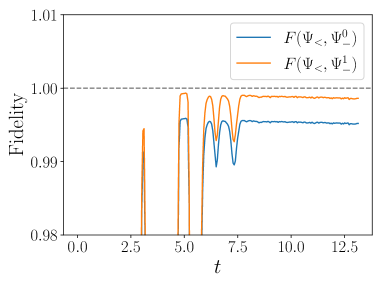
Figure 6: Fidelity  $F(\Psi_{<},\Psi_{-}^{0})$ and $F(\Psi_{<},\Psi_{-}^{1})$ between the cat component $\ket{\Psi_{<}(t)}$ and the adiabatic projections at order 0 and order 1 $|\Psi_{-}^{0/1}(t)\rangle$. After the time of separation $t_{\rm sep}\simeq 8$, the cat component $\ket{\Psi_{<}(t)}$ is very close to the lowest order adiabatic approximation $\ket{\Psi_{-}^{0}(t)}$ with a fidelity of 99.5%. The fidelity further increase with the adiabatic projection of order 1, such that $\ket{\Psi_{<}(t)}$ identifies with $\ket{\Psi_{-}(t)}$.

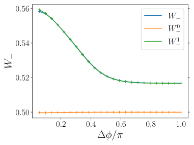
Figure 7: Effect of the difference between eigenstates and adiabatic states on the weight of the cat. Initial state of the Fig. 3(c) with $\theta_{q}=\pi/2$. In blue, weight $W_{-}$ of the cat computed dynamically from the splitting (same as Fig. 3(c)). In orange, weight $W_{-}^{0}=\innerproduct{\Psi_{-}^{0}}{\Psi_{-}^{0}}$ computed from the spectral projector $\hat{P}_{-}^{(0)}$. In green, weight $W_{-}^{1}=\innerproduct{\Psi_{-}^{1}}{\Psi_{-}^{1}}$ from the projector at order 1, which almost identifies with the weight obtained dynamically.

We show that after the time of separation $t_{\rm sep}$, the cat component which splits in the direction $n_{\perp}<n_{\perp}^{0}$ identifies with the adiabatic component $\hat{P}_{-}\ket{\Psi(t)}$ of the total state. The adiabatic projector $\hat{P}_{-}$ is constructed from the qubit’s adiabatic states $\ket{\psi_{-}(\bm{\Phi})}$ (10). It is a perturbative correction of the spectral projector $\hat{P}_{-}^{(0)}$ of the qubit Hamiltonian $H(\hat{\bm{\Phi}})$ constructed form the eigenstates $\ket{\psi_{-}^{0}(\bm{\Phi})}$.

We note $\hat{P}_{<}$ the projector on the states $\ket{n_{1}}\otimes\ket{n_{2}}\otimes\ket{s}$ with $n_{\perp}=(-\omega_{2}n_{1}+\omega_{1}n_{2})/|\bm{\omega}|<n_{\perp}^{0}$, $s=\uparrow_{z},\downarrow_{z}$, and $\ket{\Psi_{<}(t)}=\hat{P}_{<}\ket{\Psi(t)}$ the component of the system on this region $n_{\perp}<n_{\perp}^{0}$. The adiabatic projector $\hat{P}_{-}$ is constructed numerically at order 0 $\hat{P}_{-}^{(0)}=\hat{P}_{-,0}$ and at order 1 $\hat{P}_{-}^{(1)}=\hat{P}_{-,0}+\hat{P}_{-,1}$ from the expressions (74) and (77). We note respectively $\ket{\Psi_{-}^{0}(t)}=\hat{P}_{-}^{(0)}\ket{\Psi(t)}$ and $\ket{\Psi_{-}^{1}(t)}=\hat{P}_{-}^{(1)}\ket{\Psi(t)}$ the adiabatic projections respectively at order 0 and order 1 of the total state $\ket{\Psi(t)}$.

We note $F(\Psi_{1},\Psi_{2})=\innerproduct{\Psi_{1}}{\Psi_{2}}/(\innerproduct{\Psi_{1}}{\Psi_{1}}\innerproduct{\Psi_{2}}{\Psi_{2}})$ the fidelity between two states $\ket{\Psi_{1}}$ and $\ket{\Psi_{2}}$. The figure 6 represents the fidelity $F(\Psi_{<},\Psi_{-}^{0})$ and $F(\Psi_{<},\Psi_{-}^{1})$ between the cat component $\ket{\Psi_{<}(t)}$ and the adiabatic projections at order 0 and order 1. After the time of separation $t_{\rm sep}\simeq 8$, the cat component has a fidelity of approximately $99.5\%$ with $\ket{\Psi_{-}^{0}(t)}$ and $99.9\%$ with $\ket{\Psi_{-}^{1}(t)}$. The adiabatic projection at order 0 gives a very good approximation of the cat component, corrected at higher orders to gives the full adiabatic component $\ket{\Psi_{-}(t)}$. The slight decrease with time of the fidelity after the time of separation is due to the successive Landau-Zener transitions.

The difference between the adiabatic projector $\hat{P}_{-}$ and the spectral projector $\hat{P}_{-}^{(0)}$ is visible in the weight of the cat state. We represent on Fig. 7 the weight of the adiabatic projection computed dynamically from the splitting $W_{-}=\innerproduct{\Psi_{<}(t_{\rm sep})}{\Psi_{<}(t_{\rm sep})}$, and the weight $W_{-}^{0}=\innerproduct{\Psi_{-}^{0}}{\Psi_{-}^{0}}$ and $W_{-}^{1}=\innerproduct{\Psi_{-}^{1}}{\Psi_{-}^{1}}$ computed numerically from the projection of the initial state respectively at order 0 and order 1. The initial state is a Gaussian state centered on $\bm{\Phi}^{0}=(0,0)$ and the qubit in $\varphi_{q}=0$, $\theta_{q}=\pi/2$. As discussed in Sec. II.3.2, the corresponding average ground state $\bar{\bm{b}}_{-}^{0}$ lies on the $z$-axis for all $\Delta\phi$ such that $W_{-}^{0}=\frac{1}{2}$. The first order correction $W_{-}^{1}$ almost identifies with the weight obtained dynamically $W_{-}$.

Appendix H Purity from initial Fock state

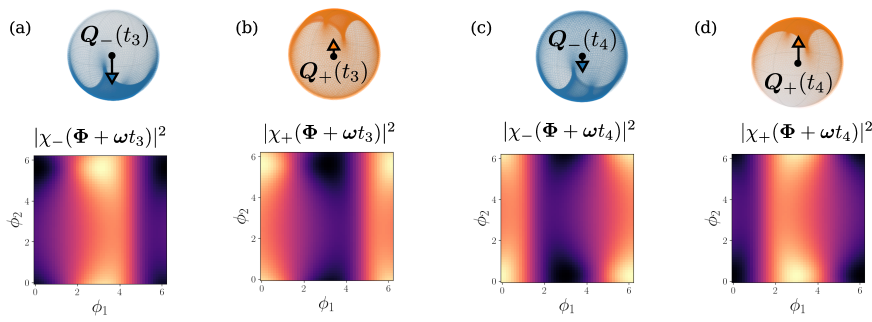
Figure 8: Phase densities $|\chi_{\pm}(\bm{\Phi}-\bm{\omega}t)|^{2}$ of the cat components $\ket{\Psi_{\pm}(t)}$ translated to densities of adiabatic states on the Bloch sphere via the map $\bm{\Phi}\mapsto\bm{b}_{\pm}(\bm{\Phi})$. The polarization of the qubit $\bm{Q}_{\pm}(t)$ is the average of adiabatic states with respect to these densities.

We illustrate the role of the phase densities in the entanglement between the qubit and the modes in the cat components $\ket{\Psi_{\pm}(t)}$ for a quasi-Fock initial state $\Delta\phi=\pi$, and the qubit initialized in $\theta_{q}=\pi/2$, $\varphi_{q}=0$. As discussed in Sec. III.1.2, for an initial quasi-Fock state the phase densities $|\chi_{\pm}(\bm{\Phi}+\bm{\omega}t)|^{2}$ of the two components of the cat split the torus in two complementary supports of equal weight. We represent these densities on Fig. 8 at the time $t=t_{3}$ and $t=t_{4}$ indicated on Fig. 4(b2). The densities on the torus translate into densities of adiabatic states on the Bloch sphere via the map $\bm{\Phi}\mapsto\bm{b}_{\pm}(\bm{\Phi})$.

At $t=t_{3}$, $|\chi_{-}(\bm{\Phi}+\bm{\omega}t_{3})|^{2}$ covers a smaller part of the Bloch sphere than $|\chi_{+}(\bm{\Phi}+\bm{\omega}t_{3})|^{2}$, such that the qubit is more entangled with the modes in $\ket{\Psi_{+}(t_{3})}$ than in $\ket{\Psi_{-}(t_{3})}$: $|\bm{Q}_{+}(t_{3})|<|\bm{Q}_{-}(t_{3})|$. During the dynamics, the phase densities are translated on the torus with no dispersion, changing the densities on the Bloch sphere and the purity of the qubit. At $t=t_{4}$, the domains have been almost exchanged $|\chi_{-}(\bm{\Phi}-\bm{\omega}t_{4})|^{2}\simeq|\chi_{+}(\bm{\Phi}-\bm{\omega}t_{3})|^{2}$, such that $\bm{Q}_{-}(t_{4})\simeq-\bm{Q}_{+}(t_{3})$ and $\bm{Q}_{+}(t_{4})\simeq-\bm{Q}_{-}(t_{3})$.

For the figures, the densities are computed from the eigenstates $\ket{\psi_{-}^{0}(\bm{\Phi})}$.

Appendix I Time evolution of the quantum fluctuations

We derive the time evolution of the quantum fluctuation, or spreading, of the modes’ number of quanta in an adiabatic component $\ket{\Psi_{\nu}(t)}$ (12)

$$[\Delta_{Q}\hat{n}_{i}(t)]^{2}=\langle\hat{n}_{i}^{2}\rangle_{\Psi_{\nu}(t)}-\langle\hat{n}_{i}\rangle_{\Psi_{\nu}(t)}^{2}$$ (78)

with $\langle\hat{\mathcal{O}}\rangle_{\Psi_{\nu}(t)}=\bra{\Psi_{\nu}(t)}\hat{\mathcal{O}}\ket{\Psi_{\nu}(t)}/\innerproduct{\Psi_{\nu}(t)}{\Psi_{\nu}(t)}$, and $i=1,2$. We show that due the linearity in $\hat{\bm{N}}$ of the Hamiltonian we can relate these quantum fluctuations to the variance of the classical trajectories $n_{i}(t;\bm{\Phi})$ [14, 23] which are obtained in an hybrid classical-quantum description of the qubit-mode coupling

$$n_{i}(t,\bm{\Phi})$$

$$=\int_{0}^{t}\differential t^{\prime}\left(\frac{1}{\hbar}\frac{\partial E_{\nu}}{\partial\phi_{i}}(\bm{\Phi}-\bm{\omega}t^{\prime})+\sum_{j}\omega_{j}F_{\nu,ij}(\bm{\Phi}-\bm{\omega}t^{\prime})\right).$$ (79)

According to (61) the time evolution of the adiabatic component is given by

$$\ket{\Psi_{\nu}(t)}=\int\differential^{2}\bm{\Phi}~{}\xi_{\nu}(t,\bm{\Phi})\ket{\bm{\Phi}-\bm{\omega}t}\otimes\ket{\psi_{\nu}(\bm{\Phi}-\bm{\omega}t)}$$ (80)

with

$$\xi_{\nu}(t,\bm{\Phi})=\tilde{\chi}_{\nu}(\bm{\Phi})e^{i\theta_{\nu}(t;\bm{\Phi})},$$ (81)

$\tilde{\chi}_{\nu}(\bm{\Phi})=\chi_{\nu}(\bm{\Phi})/W_{\nu}$ the normalized wave-function of the decomposition (11) of the initial state and $\theta_{\nu}(t;\bm{\Phi})$ the phase factor (57). This form of the time evolution is due to the linearity in $\bm{N}$ of the Hamiltonian: the phase density is translated without dispersion and the acquired phase $\theta_{\nu}(t;\bm{\Phi})$ is given by the energy function $E_{\nu}(\bm{\Phi})$ (58) and the connection $A_{\nu,i}(\bm{\Phi})$ (59).

As derived in appendix D, the time evolution of the average number of quanta reduces to a statistical average of the classical trajectories with respect to the initial phase density $|\tilde{\chi}_{\nu}(\bm{\Phi})|^{2}$

$$\langle\hat{n}_{i}\rangle_{\Psi_{\nu}(t)}=\langle\hat{n}_{i}\rangle_{\Psi_{\nu}(t=0)}+\int\differential^{2}\bm{\Phi}~{}|\tilde{\chi}_{\nu}(\bm{\Phi})|^{2}n_{i}(t,\bm{\Phi}).$$ (82)

Using $\bra{\phi_{i}^{\prime}}\hat{n}_{i}\ket{\phi_{i}}=-i\partial_{\phi_{i}}\delta(\phi_{i}^{\prime}-\phi_{i})$, we get after a few lines

$$\langle\hat{n}_{i}^{2}\rangle_{\Psi_{\nu}(t)} =\int\differential\bm{\Phi}~{}\xi_{\nu}(t,\bm{\Phi})^{*}\left(i\frac{\partial}{\partial\phi_{i}}+A_{\nu,i}(\bm{\Phi}-\bm{\omega}t)\right)^{2}\xi_{\nu}(t,\bm{\Phi})$$

$$+\int\differential^{2}\bm{\Phi}~{}|\xi_{\nu}(t,\bm{\Phi})|^{2}g_{\nu,ii}(\bm{\Phi}-\bm{\omega}t)$$ (83)

with $g_{\nu,ii}$ the quantum metric of the adiabatic states (22). Let us comment this equation. In a single band approximation of Bloch oscillations, we ignore the rotation of the states $\ket{\psi_{\nu}(\bm{\Phi})}$ such that we assume that $\xi_{\nu}(t,\bm{\Phi})$ is the wavefunction of the modes ignoring the role of the projection $\hat{P}_{\nu}$. The average value of $\hat{n}_{i}^{2}$ is then given by (I) without the connection $A_{\nu,i}$ and the metric $g_{\nu,ii}$. Here the first line corresponds to the average value of the projected observable $(\hat{P}_{\nu}\hat{n}_{i}\hat{P}_{\nu})^{2}$, where $\hat{P}_{\nu}\hat{n}_{i}\hat{P}_{\nu}$ reduces to a covariant derivative with the connection $A_{\nu,i}$ in the representation $\ket{\bm{\Phi}}\otimes\ket{\psi_{\nu}(\bm{\Phi})}$. The second term involving the quantum metric originates from the difference between the observables and the projected observables

$$\hat{P}_{\nu}\hat{n}_{i}^{2}\hat{P}_{\nu}=(\hat{P}_{\nu}\hat{n}_{i}\hat{P}_{\nu})^{2}+\hat{P}_{\nu}\hat{n}_{i}(1-\hat{P}_{\nu})\hat{n}_{i}\hat{P}_{\nu},$$ (84)

such that we show $\langle\hat{P}_{\nu}\hat{n}_{i}(1-\hat{P}_{\nu})\hat{n}_{i}\hat{P}_{\nu}\rangle=\int\differential^{2}\bm{\Phi}|\xi_{\nu}(t,\bm{\Phi})|^{2}g_{\nu,ii}(\bm{\Phi}-\bm{\omega}t)$.

We express the time evolution (I) it terms of the classical trajectories $n_{i}(t,\bm{\Phi})$ (I). Using $A_{\nu,i}(\bm{\Phi}-\bm{\omega}t)-A_{\nu,i}(\bm{\Phi})=\int_{0}^{t}\differential t^{\prime}\sum_{j}\omega_{j}\partial_{j}A_{\nu,j}(\bm{\Phi}-\bm{\omega}t^{\prime})$ and $F_{\nu,ij}=\partial_{i}A_{\nu,j}-\partial_{j}A_{\nu,i}$, these trajectories can be expressed in term of the phase factor $\theta_{\nu}(t,\bm{\Phi})$ (57)

$$n_{i}(t,\bm{\Phi})=-\frac{\partial\theta_{\nu}}{\partial\phi_{i}}(\bm{\Phi};t)+A_{\nu,i}(\bm{\Phi}-\bm{\omega}t)-A_{\nu,i}(\bm{\Phi}),$$ (85)

such that after developing the time evolution (81) of the wavefunction $\xi_{\nu}(t,\bm{\Phi})$ we obtain

$$\langle\hat{n}_{i}^{2}\rangle_{\Psi_{\nu}(t)} =\int\differential^{2}\bm{\Phi}~{}\tilde{\chi}_{\nu}(\bm{\Phi})^{*}\left(i\frac{\partial}{\partial\phi_{i}}+A_{\nu,i}(\bm{\Phi})\right)^{2}\tilde{\chi}_{\nu}(\bm{\Phi})$$

$$~{}~{}~{}+\int\differential^{2}\bm{\Phi}~{}|\tilde{\chi}_{\nu}(\bm{\Phi})|^{2}n_{i}(t,\bm{\Phi})$$

$$~{}~{}~{}+2\int\differential^{2}\bm{\Phi}~{}J_{\nu,i}(\bm{\Phi})n_{i}(t,\bm{\Phi})$$

$$~{}~{}~{}+\int\differential^{2}\bm{\Phi}~{}|\tilde{\chi}_{\nu}(\bm{\Phi})|^{2}g_{\nu,ii}(\bm{\Phi}-\bm{\omega}t)$$ (86)

$$=\langle\hat{n}_{i}^{2}\rangle_{\Psi_{\nu}(t=0)}+\int\differential^{2}\bm{\Phi}~{}|\tilde{\chi}_{\nu}(\bm{\Phi})|^{2}n_{i}(t,\bm{\Phi})$$

$$~{}~{}~{}+2\int\differential^{2}\bm{\Phi}~{}J_{\nu,i}(\bm{\Phi})n_{i}(t,\bm{\Phi})$$

$$~{}~{}~{}+\int\differential^{2}\bm{\Phi}~{}|\tilde{\chi}_{\nu}(\bm{\Phi})|^{2}(g_{\nu,ii}(\bm{\Phi}-\bm{\omega}t)-g_{\nu,ii}(\bm{\Phi}))$$ (87)

with the current density of the initial state

$$J_{\nu,i} =\frac{i}{2}\left(\tilde{\chi}_{\nu}^{*}\frac{\partial\tilde{\chi}_{\nu}}{\partial\phi_{i}}-\tilde{\chi}_{\nu}\frac{\partial\tilde{\chi}_{\nu}^{*}}{\partial\phi_{i}}\right)+|\tilde{\chi}_{\nu}|^{2}A_{\nu,i}$$ (88)

satisfying $\langle\hat{n}_{i}\rangle_{\Psi_{\nu}(t=0)}=\int J_{\nu,i}(\bm{\Phi})\differential\bm{\Phi}$.

As a result, the time evolution of the spreading is given by the variance (33) of the classical trajectories and by two other terms

$$[(\Delta_{Q} \hat{n}_{i})(t)]^{2}=[(\Delta_{Q}\hat{n}_{i})(t=0)]^{2}+\text{Var}_{|\chi_{\nu}|^{2}}[n_{i}(t,\bm{\Phi})]$$

$$+\int\differential\bm{\Phi}~{}|\tilde{\chi}_{\nu}(\bm{\Phi})|^{2}\left(g_{\nu,ii}(\bm{\Phi}-\bm{\omega}t)-g_{\nu,ii}(\bm{\Phi})\right)$$

$$+\delta C_{i}(t).$$ (89)

where $\delta C_{i}(t)$ is a bounded term taking the form of correlations between the classical trajectories $n_{i}(t,\bm{\Phi})$ and a current density of the initial state $J_{\nu,i}(\bm{\Phi})$

$$\delta C_{i}(t)= 2\int\differential^{2}\bm{\Phi}~{}J_{\nu,i}(\bm{\Phi})n_{i}(t,\bm{\Phi})$$ (90)

$$-2\langle\hat{n}_{i}\rangle_{\Psi_{\nu}(t=0)}\int\differential^{2}\bm{\Phi}~{}|\tilde{\chi}_{\nu}(\bm{\Phi})|^{2}n_{i}(t,\bm{\Phi})$$ (91)

As discussed above, the classical trajectories $n_{i}(t,\bm{\Phi})$ characterize the spreading of the projected observables $\hat{P}_{\nu}\hat{n}_{i}\hat{P}_{\nu}$, and the quantum metric relates the spreading of the projected and non-projected observables. Concerning Bloch oscillations and Bloch breathing, the important feature of this quantum metric contribution is that it is small compared to the initial value $[(\Delta_{Q}\hat{n}_{i})(t=0)]^{2}$ in the case of small $\Delta\phi$, and it is vanishingly small at quasi-periods $T$ such that $\bm{\Phi}-\bm{\omega}T\simeq\bm{\Phi}$. The last term $\delta C_{i}(t)$ has the same features. It is vanishingly small at quasi-periods $T$ since $n_{i}(T,\bm{\Phi})\simeq 0$. It is also small in the small $\Delta\phi$ limit since it can be written as classical correlations with respect to the density $|\tilde{\chi}_{\nu}(\bm{\Phi})|^{2}$ between the function $\partial_{i}\alpha(\bm{\Phi})+A_{\nu,i}(\bm{\Phi})$ and $n_{i}(t,\bm{\Phi})$, with $\alpha(\bm{\Phi})$ the complex argument of $\tilde{\chi}_{\nu}(\bm{\Phi})$.

We thus recover the behaviors of Bloch oscillations and Bloch breathing discuss in Sec. III.2: the spreading of the cat component remains almost constant $(\Delta_{Q}\hat{n}_{i})(t)\simeq(\Delta_{Q}\hat{n}_{i})(t=0)$ in the case of localization in phase $\Delta\phi\ll 1$, and it refocuses at quasi-period $T$, $(\Delta_{Q}\hat{n}_{i})(T)\simeq(\Delta_{Q}\hat{n}_{i})(t=0)$ irrespective to the value of $\Delta\phi$.