A New Spatio-Temporal Model Exploiting Hamiltonian Equations

Abstract

The solutions of Hamiltonian equations are known to describe the underlying phase space of the mechanical system. Hamiltonian Monte Carlo is the sole use of the properties of solutions to the Hamiltonian equations in Bayesian statistics. In this article, we propose a novel spatio-temporal model using a strategic modification of the Hamiltonian equations, incorporating appropriate stochasticity via Gaussian processes. The resultant sptaio-temporal process, continuously varying with time, turns out to be nonparametric, nonstationary, nonseparable and non-Gaussian. Additionally, as the spatio-temporal lag goes to infinity, the lagged correlations converge to zero. We investigate the theoretical properties of the new spatio-temporal process, including its continuity and smoothness properties. In the Bayesian paradigm, we derive methods for complete Bayesian inference using MCMC techniques. The performance of our method has been compared with that of non-stationary Gaussian process (GP) using two simulation studies, where our method shows a significant improvement over the non-stationary GP. Further, application of our new model to two real data sets revealed encouraging performance.

Keywords: Continuously varying time and space; Hamiltonian dynamics; Markov Chain Monte Carlo; Non-stationarity; Non-Gaussianity; Spatio-temporal modeling;

1 Introduction

Modeling spatially and spatio-temporally dependent data drew much attention in the last few decades within the statistics community. Numerous scientific disciplines, such as meteorology [1, 2, 3, 4, 5, 6, 7, 8, 9]), environment [10, 11, 12, 13, 14, 15, 16, 17] and ecology [18, 19], give rise to challenging spatio-temporal data. The goal of modeling spatio-temporal data is to predict values of the underlying spatio-temporal process at desired locations and future time points. Two common assumptions are employed while analyzing spatio-temporal data: (i) separability of the covariance function in space and time (for definition of separability, see Chapter 11 of [20]), and (ii) covariance stationarity. By covariance stationarity, we mean that the covariance of the observations at any two locations and time points is a function of the separation vector between the two locations and time points (Chapters 2 and 11 of [20]). A special case of covariance stationarity, known as isotropic stationarity, is also typically assumed while analyzing spatial and spatio-temporal data. By isotropic stationarity one implies that the covariance between two spatio-temporal observations is a function of the distance between the corresponding locations and time points (Chapters 2 and 11 of [20]). However, in reality assumptions of any kind of stationary can be artificial if there is local influence on the correlation structure [21]. Indeed, the scenario of local influence is not uncommon in practice. [22] and [23] showed that the PM10 pollution data set, analyzed by [16], is not stationary. The same finding was established for a sea-temperature data set by [24]. Furthermore, [25] demonstrated that the erroneous assumption of a stationary covariance function would lead to an overly smoothed or underly smoothed process. For a short review on the necessity of the nonstationarity for modeling spatio-temporal data, one can see Chapter 9 of [26].

In recent times, many attempts are made to incorporate nonstationarity of the underlying spatio-temporal process. [21] first significantly contributed in capturing nonstationarity of the covariance function based on the idea of spatial deformation. This idea has been further exploited in the Bayesian paradigm by [27] and [28]. Kernel convolution technique was used by [29, 30, 31, 32, 33, 34] to model nonstationarity of the underlying processes. A significant amount of work is also done towards formulating the nonstationary processes via stochastic partial differential equation (SPDE) approach. SPDE approach in modeling spatial data was first proposed by [35]. [35] represents a continuous spatial process, a Gaussian field (GF) as a Gaussian Markov random field (GMRF), a discretely indexed spatial random field. The key ingredient was to use the fact that a GF with Matérn covariance kernel is the solution of a fractional SPDE (Chapter 6 of [36]). Within the framework of SPDE appraoch, the extension to nonstationary covariance function can easily be done by varying the parameters of Matérn covariance kernel with the locations ([35, 37, 38] and [36]). A lucid review on SPDE approach in modeling spatial and spatio-temporal data is provided in [39]. One major advantage of using SPDE approach is the availability of INLA package in statistical software R due to [40]. The INLA package can efficiently analyze spatial and spatio-temporal data using stationary and nonstationary processes via SPDE approach. The books [36], [41] and the website r-inla.org/home provide a detailed overview of the package INLA. Another advantage of SPDE approach is that it can be applied to a data set with a large number of locations and time points as it deals with sparse matrices (see Chapter 6 of [36]). In a different direction, with the help of Dirichlet process, [42] attempted to model the underlying spatial process nonparametrically along with “conditional” nonstationarity. Further, a nonparametric and nonstationary model was proposed by [43] using kernel process mixing. A discretized version of a stochastic differential equation is considered by [44] to model spatio-temporal nonstationarity.

In majority of these above mentioned work, two aspects can be noticed. Either, the underlying process is Gaussian (may be nonstationary), or the correlation between the two spatio-temporal points was not shown to converge to 0 as the distance between the two points (locations and/or time points) increases to infinity, or both. It is not very unlikely to realize spatio-temporal data those are not Gaussian (see for example, [43], [22], [24] etc). Moreover, in many real life applications often it is observed that the sample correlation goes to zero as the distance between two spatial locations and/or two time points goes to infinity (see for example [24]). For a stationary spatio-temporal process it comes naturally from the structure of the covariance function. Hence, while proposing a non-stationary spatio-temporal process, it is desirable to ensure convergence of the correlation to 0 as the distance between two locations and/or time points increases to infinity. Very recently, [22] proposed a nonparametric, non-separable, nonstationary and non-Gaussian spatio-temporal model based on order-based dependent Dirichlet process, where they showed that the underlying covariance function goes to 0 as the distance between the two locations and/or time points increases to infinity. While modeling spatio-temporal data, [22] also assumed that time and the space vary continuously in their respective domains. Although [22] made a successful attempt building the nonparametric, nonstationary, non-Gaussian model with the desirable properties of covariance, this model does not impart dynamic properties to the temporal part, either directly or via any latent process. It is well known that a statistical model intended for explaining temporal variability should evolve dynamically (Chapter 1 of [45]). On the other hand, [46] introduces a nonparametric spatio-temporal model, which, through a nonparametric dynamic latent process, induces desirable dynamic properties in the temporal part. In addition, the model of [46] is nonstationary. However, time does not vary continuously on the respective domain.

In a nutshell, there does not seem to exist any nonparametric, nonstationary, non-separable, non-Gaussian, dynamic spatio-temporal model, which is continuous in time and space with an underlying structured latent process, and with the property that the correlation between two spatio-temporal vatiables goes to 0 as the spatial/temporal lag goes to infinity. To fill up this gap we propose a dynamic spatio-temporal nonparametric, non-Gaussian model, where the underlying process is nonstationary. A structured latent process is incorporated in the proposed model. The time and the space in our proposed spatio-temporal model vary continuously over their respective domains. Further, the underlying process enjoys the property that the covariance goes to 0 as the spatial/temporal lag tends to infinity.

For constructing the model proposal, we invoke the Hamiltonian dynamics from physics. Hamiltonian equations are applied to Bayesian statistics in formulating Hamiltonian Monte Carlo [47, 48]. However, formulation of spatio-temporal model exploiting the idea of the Hamiltonian dynamics is not considered earlier. The solution of the Hamiltonian equations describes the phase-space of a mechanical space. Moreover, the solutions, which are inter-dependent, continuously vary with respect to time. These properties motivates us to construct a spatio-temporal model based on the solutions of Hamiltonian equations, after some modifications (see Section 2), with desirable properties. We first briefly describe the Hamiltonian dynamics and the equations. Thereafter, we shall connect the idea of the spatio-temporal model to Hamiltonian dynamics. In the latter section (Section 2) we describe the mathematical formulation in detail.

Let $(\mathcal{M},\mathcal{L})$ be a mechanical system, where $\mathcal{M}$ is the configuration space and $\mathcal{L}$ is the smooth Lagrangian. The coordinate system of $\mathcal{M}$ is determined by $(\theta,\dot{\theta})$, where $\theta$ is the position of a particle at time $t$ and the $\dot{\theta}$ is the derivative vector with respect to time, thus representing the velocity. The partial derivative of $\mathcal{L}$ with respect to $\dot{\theta}$, known as momenta, is denoted by $p$, which is a function of time $t$, the position $\theta$, and velocity $\dot{\theta}$. Now the Hamiltonian, a function of ${p}$, $\theta$ and $t$, is defined as

$${H}(p,\theta,t)=\sum_{i}p_{i}\dot{\theta}_{i}-\mathcal{L}(\theta,\dot{\theta},t),$$

which is the energy function of the mechanical system. Here $p_{i}\text{ and }\dot{\theta}_{i}$ are the $i$th component of $p$ and $\dot{\theta}$. The pair $(\theta,p)$ is called phase space coordinates. The phase space coordinates are the solution of the Hamiltonian equations

$$\frac{d\theta}{dt}=\frac{\partial{H}}{\partial{p}},\text{ and }\frac{d{p}}{dt}=-\frac{\partial{H}}{\partial\theta}.$$

We note here that the solution $\theta$, which describes the position of a particle at time $t$ and depends on $p$, the other coordinate of the phase-space, varies continuously with respect to time. Further, $p$ is also dependent on $\theta$ at time $t$, and varies continuously with respect time $t$. In our case, we introduce $p(t)$ as the latent and $\theta(t)$ as the observed spatio-temporal processes with the hope that the solution to Hamilton’s equations will best describe the underlying state-space as done in the phase-space of the mechanical space. To obtain the solution of Hamilton’s equations, one can invoke the leap-frog algorithm [49]. In this article, we propose a modified leap-frog algorithm associated with modification of the Hamiltonian equations to build our spatio-temporal model incorporating the latent and the observed processes, which continuously depend on time $t$. Moreover, since the leap-frog algorithm exploits the presence of derivative, our proposed spatio-temporal model also enjoys dynamic property with respect to time $t$ through its previous time point $t-\delta t$. The Bayesian nonparametric flavour of our approach is due to modeling functions with unknown forms in the Hamiltonian equations by appropriate Gaussian processes. In turn, it is observed that the desirable properties, non-stationarity, non-separability, non-Gaussianity are satisfied. Further analysis shows that the covariance function of the proposed process goes to 0 as the spatial and/or temporal lag tends to infinity.

The remaining part of the article is planned in the following manner. In Section 2, we propose our new spatio-temporal process based on modified Hamiltonian equations and modified leap-frog algorithm. Section 2 presents the important and necessary properties of the proposed observed and latent processes. The proofs of the lemmas, theorems and corollaries, discussed in Section 2, are given in Section S-1 of Supplementary Information. The likelihood function of the parameter vector involved in the model is provided in Section 3. In this section we first find out the joint conditional density of the data given the latent variables and the parameters (Subsection 3.1 and Section S-2 of Supplementary Information) and then obtain the joint density of latent variables given the observed data and the parameters (Subsection 3.2 and Section S-3 of Supplementary Information), before presenting the complete likelihood of the parameter vector (Subsection 3.3). Section 4 deals with the choice of prior distributions for the parameter vectors. A plausible justification of the choice of the prior distributions is also discussed in this section. For applying Gibbs sampling, we evaluate the full conditional densities of all the parameters along with the latent variables in Section 5. The detailed calculation of the full conditional densities are given in Section S-4 of Supplementary Information. Simulation studies and the real data analysis are given in the Sections 6 and 7, respectively. In Section 6, we provide the results of two simulations studies. The findings of our model for these simulation experiments are compared with those of a nonstationary Gaussian process, which was fit using the SPDE approach following [35] using INLA [40]. In Section 7, two real data sets are analyzed to show the performance of the newly proposed spatio-temporal model. Among these two real data sets, one of the data sets corresponds to nonstationary and non-Gaussian, while another is associated with a stationary non-Gaussian spatio-temporal process. Finally, in Section 8, we summarize our contributions and make concluding remarks.

2 Modified Hamiltonian equations and the proposed model

2.1 Modified Hamiltonian equations and the corresponding leap-frog algorithm

We first provide the foundation of forming spatio-temporal model from modified Hamiltonian equations and the corresponding Leap-frog algorithm. Let the total energy of a mechanical system, known as Hamiltonian function, be denoted by $H(p,\theta)$. Assume that $H(p,\theta)=V(\theta)+W(p)$, where $V(\theta)$ is the potential energy, $W(p)$ is the kinetic energy given as $W(p)=\frac{1}{2}p^{T}M^{-1}p$, with $M$ being a chosen matrix (mass), and ($\theta,p$) are phase space coordinates (depends on time $t$) [48]. Then the original Hamiltonian equations are given by

$$\frac{dp}{dt} =\frac{-\partial H}{\partial\theta}=-\nabla V(\theta)\mbox{ and }$$

$$\frac{d\theta}{dt} =\frac{\partial H}{\partial p}=M^{-1}p,$$

where by $\nabla V(\theta)$ we mean gradient of $V$ with respect to $\theta$. The leap-frog algorithm for numerically solving the Hamiltonian equations is given by

$$\theta(t+\delta t) =\theta(t)+\delta tM^{-1}\left\{p(t)-\frac{1}{2}\delta t\nabla V(\theta(t))\right\}\mbox{ and }$$

$$p(t+\delta t) =p(t)-\frac{1}{2}\delta t\left[\nabla V(\theta(t))+\nabla V(\theta(t+\delta t))\right].$$

We modify the original Hamiltonian equations so that the rate of change of $p$ and $\theta$ with respect to $t$ depends on $p$ and $\theta$ both. The easiest way to do so, is to incorporate $p$ and $\theta$ linearly in the equation of $\frac{dp}{dt}$ and $\frac{d\theta}{dt}$, respectively. That is, Hamiltonian equations are modified to

$$\frac{dp}{dt} =\alpha^{*}p-\nabla V(\theta)\mbox{ and }$$

$$\frac{d\theta}{dt} =\beta^{*}\theta+M^{-1}p.$$

Accordingly, the leap-frog algorithm is modified and is given below. Using Leap-frog algorithm for $\theta$ [49], we have

$$\theta(t+\delta t) =\theta(t)+\beta^{*}\theta(t)\delta t+\delta tM^{-1}p(t+\delta t/2)$$

$$=\theta(t)\left(1+\beta^{*}\delta t\right)+\delta tM^{-1}p(t+\delta t/2)$$

$$=\beta\theta(t)+\delta tM^{-1}p(t+\delta t/2),$$ (1)

where $\beta=\left(1+\beta^{*}\delta t\right).$ We set $|\beta|<1$, which implies $-2<\beta^{*}\delta t<0$. As will be seen subsequently, this restriction is necessary for the lagged correlations between the observations to tend to zero as the space-time lag tends to infinity. Now, for $p$, a numerical approximation can be done as

$$p\left(t+\frac{\delta t}{2}\right) =p(t)+\alpha^{*}p(t)\frac{\delta t}{2}-\nabla V(\theta(t))\frac{\delta t}{2}$$

$$=p(t)\left(1+\alpha^{*}\frac{\delta t}{2}\right)-\nabla V(\theta(t))\frac{\delta t}{2}$$

$$=\alpha p(t)-\nabla V(\theta(t))\frac{\delta t}{2},$$ (2)

where $\alpha=\left(1+\alpha^{*}\frac{\delta t}{2}\right)$. We set $|\alpha|<1$ implying $-2<\alpha^{*}\frac{\delta t}{2}<0$. Restricting $\alpha$ on $(-1,1)$ led to good MCMC mixing in our Bayesian applications. Replacing equation (2.1) into equation (2.1), we obtain

$$\theta(t+\delta t) =\beta\theta(t)+\delta tM^{-1}\left(\alpha p(t)-\nabla V(\theta(t))\frac{\delta t}{2}\right)$$ (3)

Again, invoking leap-frog algorithm for $p$ (see [49]), we obtain

$$p(t+\delta t) =p(t+\delta t/2)+\alpha^{*}p(t+\delta t/2)\frac{\delta t}{2}-\nabla V\left(\theta({t+\delta t})\right)\frac{\delta t}{2}$$

$$=p(t+\delta t/2)\left(1+\alpha^{*}\frac{\delta t}{2}\right)-\nabla V\left(\theta({t+\delta t})\right)\frac{\delta t}{2}$$

$$=\alpha p(t+\delta t/2)-\nabla V\left(\theta({t+\delta t})\right)\frac{\delta t}{2}$$

$$=\alpha\left(\alpha p(t)-\nabla V(\theta(t))\frac{\delta t}{2}\right)-\nabla V\left(\theta({t+\delta t})\right)\frac{\delta t}{2}$$

$$=\alpha^{2}p(t)-\frac{\delta t}{2}\left\{\alpha\nabla V(\theta(t))+\nabla V(\theta({t+\delta t}))\right\},$$ (4)

where the fourth equality of equation (2.1) follows from equation (2.1). Equations (2.1) and (3) constitute the modified leap-frog equations and are the key ingredients of our proposed spatio-temporal process.

2.2 Proposed model

This subsection proposes the spatio-temporal model via equations (3) and (2.1). Let $y(s,t)$ be a realization of the stochastic process $\{Y(s,t):s\in S,t\geq 0\}$, where $S\subset\mathbb{R}^{2}$, non-empty, containing a rectangle of positive volume. Also assume that corresponding to $y(s,t)$ there is a latent variable $x(s,t)$, which is a realization of a process $\{X(s,t):s\in S,t\geq 0\}$. However, unlike $y(s,t)$, $x(s,t)$ is not observed. For location $s\in S$, where $S$ is a nonempty subset of $\mathbb{R}^{2}$, replacing $\theta(t)$, $p(t)$, $M$ and $\nabla V(\theta(t))$ by $y(s,t)$, $x(s,t)$, $M_{s}$ and $\frac{d}{dx}V(x)\bigg{|}_{x=y(s,t)}$ in equations (2.1) and (3), we propose the spatio-temporal model as

$$y(s,t+\delta t) =\beta y(s,t)+\delta tM_{s}^{-1}\left(\alpha x(s,t)-\frac{\delta t}{2}\frac{dV}{du}(u)\bigg{|}_{u=y(s,t)}\right),$$ (5)

$$x(s,t+\delta t) =\alpha^{2}x(s,t)-\frac{\delta t}{2}\left(\alpha\frac{dV}{du}(u)\bigg{|}_{u=y(s,t)}+\frac{dV}{du}(u)\bigg{|}_{u=y(s,t+\delta t)}\right),$$ (6)

where (5) corresponds to observation equation and (6) deals with the dynamics of the latent variable. The parameters $\alpha$, $\beta$ are such that $|\alpha|<1$ and $|\beta|<1$, and $M_{s}$ is a function of $s$. The function $V(\cdot)$ is modeled as random function. Note that equation (6) is not the latent equation per se, since it involves the observed variable as well. Integrating the conditional distribution of the latent variable (equation (6)) over the observed variable would give us the latent distribution.

To complete the specification of our spatio-temporal process, we need to model the function $V(\cdot)$ as some appropriate stochastic process; we consider the Gaussian process for our purpose. The choice of Gaussian process for $V(\cdot)$, under suitable assumptions, makes $V^{\prime}(\cdot)$ Gaussian as well ([50, 51]). Due to this fact, the conditional likelihoods become available in closed forms (see Section 3). Specification of the proposed processes also requires an appropriate form for $M_{s}$. Details on these, along with investigation of the theoretical properties of our spatio-temporal processes, are provided in the next subsection.

2.3 Completion of specification of the proposed spatio-temporal process and investigation of its theoretical properties

Let $s\in S$, a compact subset of $\mathbb{R}^{2}$. We put the following assumptions on the processes $X(s,0),Y(s,0)$, $s\in S$ and the random function $V(\cdot)$.

1. $X(s,0),\,s\in S$ is assumed to be a centered Gaussian process with a symmetric, positive definite covariance function with bounded partial derivatives. For instance, the Matérn covariance function with $\nu>1$ has bounded partial derivatives, and could be employed. In particular, we consider the squared exponential covariance between $X(s_{1},0)$ and $X(s_{2},0)$, of the form $\sigma^{2}_{p}\exp{\{-\eta_{1}||s_{1}-s_{2}||^{2}\}}$, $s_{1},s_{2}\in S$.

2. $Y(s,0),\,s\in S$ is also assumed to be a centered Gaussian process with a symmetric, positive definite covariance function with bounded partial derivatives. Again, we consider the squared exponential covariance function of the form $\sigma^{2}_{\theta}\exp{\{-\eta_{2}||s_{1}-s_{2}||^{2}\}}$.

3. The function $V(\cdot)$ is assumed to be a Gaussian random function with zero mean and covariance function $c_{v}(x_{1},x_{2})=\sigma^{2}\exp{\{-\eta_{3}||x_{1}-x_{2}||^{2}\}}$. As for the other cases, different choices of covariance structure can be assumed with the assumption that covariance function is continuously twice differentiable and the mixed partial derivatives are Lipschitz continuous. If the covariance function has third bounded partial derivatives then the function will be Lipschitz. In our example, the covariance function is infinitely differentiable and the derivatives are bounded. Other choices may include rational quadratic covariance function, Matérn covariance function with $\nu>2$ among many others.

Remark 1

Above assumptions need well behaved covariance functions in the sense of smoothness. For a list of such covariance functions one may see [20]. Smoothness properties along with other important properties of Matérn covariance functions have been covered in [52] (Chapter 2).

Remark 2

The assumptions A1 and A2 imply that the covariance functions of $X(s,0)$ and $Y(s,0)$ are symmetric, positive definite and Lipschitz continuous, and thus $X(s,0)$ and $Y(s,0)$ will have continuous sample paths with probability 1. If the covariance functions are taken to be the Matérn covariance function with $\nu>1$ or the squared exponential covariance function, then $X(s,0)$ and $Y(s,0)$ will have differentiable sample paths in $s$.

Remark 3

Assumption A3 implies that the derivative process of $V(\cdot)$ is also a Gaussian process with continuous sample paths almost surely. In fact, if the squared exponential covariance function is assumed then all the derivatives of $V(\cdot)$ will be Gaussian processes. In particular, the differential of $V(\cdot)$ will have differentiable sample paths. Also note that for Matérn covariance function with $\nu>2$, the random function $V(\cdot)$ is differentiable and the corresponding covariance function is the mixed partial derivative of the covariance function of $V(\cdot)$. Moreover, the differential of $V(\cdot)$ will have differentiable sample paths as $\nu$ is assumed to be more than 2 for Matérn covariance function (refer to [51] along with [52]).

Now we propose a form of $M_{s}$ which is continuous and infinitely differentiable when defined on a compact set $S\subset\mathbb{R}^{2}$.

Definition 4 (Definition of $M_{s}$)

Let $S$ be a compact subset of $\mathbb{R}^{2}$. Define $M_{s}=\exp(\max\{||s^{2}-u^{2}||^{2}:u\in S\})$, where by $\mbox{\boldmath{$v$}}^{2}$ we mean $\mbox{\boldmath{$v$}}^{2}=(v_{1}^{2},v_{2}^{2})^{T}$, for $\mbox{\boldmath{$v$}}\in S$.

Lemma 2.1

$M_{s}$ is infinitely differentiable in $s\in S$.

Remark 5

It can be argued that $M_{s}\rightarrow\infty$ and $M_{s^{\prime}}\rightarrow\infty$ as $||s-s^{\prime}||\rightarrow\infty$ in the following fashion. Let $||s-s^{\prime}||\rightarrow\infty$ as $S$ also grows in the sense $S_{1}\subset S_{2}\subset\ldots$, such that at each stage $i$, $S_{i}$ remains compact. Under this limiting situation, $M_{s}=\exp\left(\max\{||s^{2}-u^{2}||^{2}:u\in S\}\right)\geq\exp\left(||s^{2}-s^{\prime 2}||^{2}\right)\rightarrow\infty$ and $M_{s^{\prime}}=\exp\left(\max\{||s^{\prime 2}-u^{2}||^{2}:u\in S\}\right)\geq\exp\left(||s^{\prime 2}-s^{2}||^{2}\right)\rightarrow\infty.$

The next results shows that the conditional covariance function of $\theta_{s}(t)$ given $p$ goes to 0 as the distance between two time points and two spatial locations increase to infinity. The distance between two time points and two spatial locations are measured with respect to their corresponding distance metrics.

Theorem 2.1

Under the assumptions A1 to A3, cov$\left(Y(s,h\delta t),Y(s^{\prime},h^{\prime}\delta t)\bigg{|}X\right)$ converges to 0 almost surely, as $||s-s^{\prime}||\rightarrow\infty$ and/or $|h-h^{\prime}|\rightarrow\infty$.

Remark 6

Note that by Theorem 2.1 and the dominated convergence theorem, the unconditional covariance cov $\left(Y(s,h\delta t),Y(s^{\prime},h^{\prime}\delta t)\right)\rightarrow 0$ as $||s-s^{\prime}||\rightarrow\infty$ and/or $|h-h^{\prime}|\rightarrow\infty$.

Remark 7

In Theorem 2.1, $\delta t$ in $h\delta t$ and $h^{\prime}\delta t$ make the time points continuous for continuous $\delta t$. However, discrete values of $\delta$ are also allowed.

Remark 8

The closed form of the covariance functional of our proposed process $Y(s,t)$ is not available. However, we can argue in the following way that covariance is non-stationary. Conditional on the latent variables, the covariance depends upon the latent variable. For simplicity, let us assume that latent process is supported on a compact set. Then, by mean value theorem for integrals, unconditional covariance is a function of a specific value of the latent variables. Moreover, the latent variables are almost surely nonlinear in locations and times, implying that the unconditional covariance is a nonlinear function of space and time. Therefore, it must be non-stationary.

To complete the discussion on correlation analysis, we provide a small simulation example, which provides us an idea how the spatial correlation matrix of our model will be, and how it is different from the squared exponential or Matérn covariance. In particular, the simulation study shows that the spatial correlation of the proposed model can be negative, whereas the correlation with squared exponential or Matérn covariance kernel will always be positive (see Figure 1).

We simulated spatio-temporal observations 1000 times from our model taking $\eta_{1}=\eta_{2}=\eta_{3}=1$, $\sigma^{2}=\sigma^{2}_{\theta}=\sigma_{p}^{2}=1$, $\alpha=\beta=0.9$. The number of locations and time points are taken to be 10 and 4, respectively. Based on 1000 simulations we have calculated the sample spatial correlation matrix. Similarly, we simulated spatio-temporal observations from a Gaussian process with zero mean and squared exponential kernel with the variance and the decaying parameter to be 1. The corresponding sample spatial correlation matrix is calculated based on the 1000 repetitions. The same exercise has been done by replacing the squared exponential kernel with two Matérn covariance kernels, namely, Matérn(3/2) and Matérn(5/2), respectively. The range parameter for Matérn covariance kernel is taken as 1 for both the cases. The sample spatial correlations are provided in Figure 1.

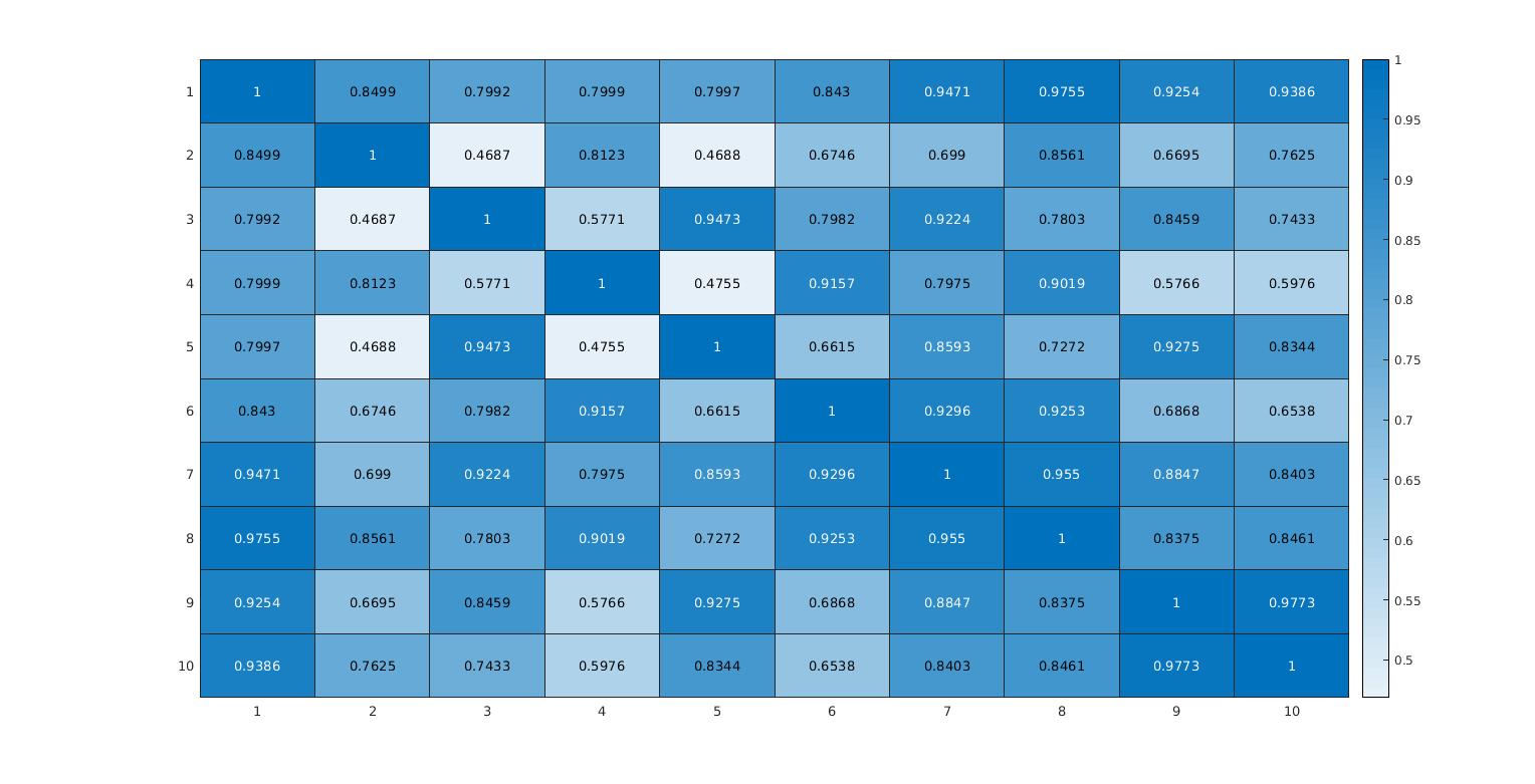
(a) Spatial correlation matrix for squared exponential.

(b) Spatial correlation matrix for Matérn(3/2).

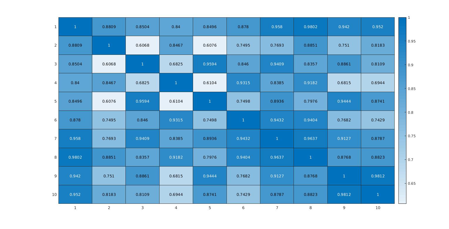
(c) Spatial correlation matrix for Matérn(5/2).

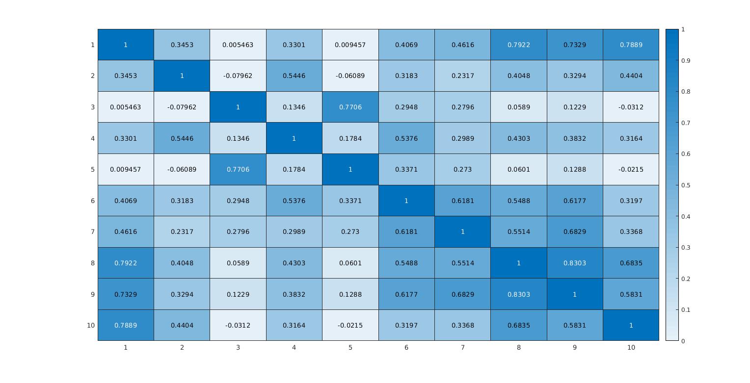
(d) Spatial correlation matrix for model.

Figure 1: The figure depicts examples of spatial correlation matrices for four different models. Our model can have negative entries in a correlation matrix whereas the correlation matrices for the other models are always positive.

Now we show that $Y(s,t)$ and $X(s,t)$ are continuous in $s$ with probability 1 and in the mean square sense. Since the (modified) Hamiltonian equations already imply that $Y(s,t)$ and $X(s,t)$ are path-wise differentiable with respect to $t$, we focus on their smoothness properties with respect to $s$.

Theorem 2.2

If the assumptions A1-A3 hold true, then $Y(s,h\delta t)$ and $X(s,h\delta t)$ are continuous in $s$, for all $h\geq 1$, with probability 1.

Theorem 2.3

Under assumptions A1-A3, $Y(s,h\delta t)$ and $X(s,h\delta t)$ are continuous in $s$ in the mean square sense, for all $h\geq 1$.

The next two results deal with differentiability of the processes $Y(s,t)$ and $X(s,t)$.

Theorem 2.4

Under assumptions A1-A3,, $Y(s,h\delta t)$ and $X(s,h\delta t)$ have differentiable sample paths with respect to $s$, almost surely.

Remark 9

Theorem 2.4 is about once differentiability, however, it can be extended to $k$ times differentiability depending on the structure of the covariances assumed on the processes $Y(s,0)$, $X(s,0)$ and the random function $V(\cdot)$. For example, if we assume squared exponential covariance functions on each process, then $Y(s,h\delta t)$ and $X(s,h\delta t)$ will have $k$ times differentiable sample paths in $s$, for any $k\in\mathbb{N}$.

For proving that the processes $Y(s,t)$ and $X(s,t)$ are mean square differentiable in $s$, we need a lemma, stated below, which may be of independent interest.

Lemma 2.2

Let $f:\mathbb{R}\rightarrow\mathbb{R}$ be a zero mean Gaussian random function with covariance function $c_{f}(x_{1},x_{2})$, $x_{1},x_{2}\in\mathbb{R}$, which is four times continuously differentiable. Let $\left\{Z(s):s\in S\right\}$ be a random process with the following properties

1. $E(Z(s))=0$,

2. covariance function $c_{Z}(s_{1},s_{2})$, $s_{1},s_{2}\in S$, where $S$ is a compact subspace of $\mathbb{R}^{2}$, is four times continuously differentiable, and

3. $\frac{\partial Z(s)}{\partial s_{i}}$ has finite fourth moment.

Then the process $\{g(s):s\in S\}$, where $g(s)=f(Z(s))$, is mean square differentiable in $s$.

Theorem 2.5

Let A1-A3 hold true, with the covariance functions of all the assumed Gaussian processes being squared exponential. Then $Y(s,h\delta t)$ and $X(s,h\delta t)$ are mean square differentiable in $s$, for every $h\geq 1$.

3 Calculation of likelihood functions

In this section we will derive the data model and the process model under assumptions A1-A3. Particularly, we assume here that the random function $V(\cdot)$ is a Gaussian process with mean 0 and squared exponential function as covariance function for simplicity of calculations. Other covariance functions (with required properties, see assumption A3) will work in the same manner. In particular, we assume that the covariance function of $V(\cdot)$ takes the form $\mbox{cov}(V(x),V(y))=k(h)=\sigma^{2}e^{-\eta_{3}h^{2}}$, where $h=||x-y||$. Then $V^{\prime}(\cdot)$ will be a Gaussian random function with mean 0 and covariance function

$$\mbox{cov}(V^{\prime}(x),V^{\prime}(y))=2\eta_{3}\sigma^{2}e^{-\eta_{3}h^{2}}(1-2\eta_{3}h^{2}),$$ (7)

(see [52], Chapter 2).

Before moving forward, we introduce a few notation which will be used for calculations of different distributions. Suppose $s_{1},\ldots,s_{n}$ denote the $n$ locations, where $s_{i}\in\mathbb{R}^{2}$, for $i=1,\ldots n$. Let observed data be given as

$$\mathbb{D}=\left\{\mbox{\boldmath{$y$}}_{1}^{T},\mbox{\boldmath{$y$}}_{2}^{T},\ldots,\mbox{\boldmath{$y$}}_{T}^{T}\right\},$$

and the corresponding latent variables be

$$\mathbb{L}=\left\{\mbox{\boldmath{$x$}}_{1}^{T},\mbox{\boldmath{$x$}}_{2}^{T},\ldots,\mbox{\boldmath{$x$}}_{T}^{T}\right\},$$

where $\mbox{\boldmath{$y$}}_{t}=(y(s_{1},t),y(s_{2},t),\ldots,y(s_{n},t))^{T}$ and $\mbox{\boldmath{$x$}}_{t}=(x(s_{1},t),x(s_{2},t),\ldots,x(s_{n},t))^{T}$ for $t=1,\ldots,T$.

Assuming $i\in\{1,\ldots,n\}$, $m\in\{0,\ldots,T\}$ and $r\in\{1,\ldots,T\}$, we define

$$h_{ij}(m) =|y(s_{i},m)-y(s_{j},m)|,$$

$$\mbox{\boldmath{$\mu$}}_{m} =(\mu_{1}(m),\ldots,\mu_{n}(m))^{T},\text{ where }\mu_{i}(m)=\beta y(s_{i},m)+\frac{\alpha x(s_{i},m)}{M_{s_{i}}},$$

$$\mbox{\boldmath{$W$}}_{r} =(V^{\prime}(y(s_{1},r)),\ldots,V^{\prime}(y(s_{n},r)))^{T},$$

$$\ell_{ik}(r-1,r) =|y(s_{i},r-1)-y(s_{k},r)|,$$

$$\mathbb{W}_{r-1} =\begin{pmatrix}\alpha\mbox{\boldmath{$W$}}_{r-1}\\ \mbox{\boldmath{$W$}}_{r}\end{pmatrix},$$

$$\theta =(\alpha,\beta,\sigma^{2},\sigma_{\theta}^{2},\sigma_{p}^{2},\eta_{1},\eta_{2},\eta_{3}).$$

By ${\mbox{\boldmath{$a$}}}^{T}$, we mean transpose of a vector $a$ and by $f^{\prime}$ we mean derivative of $f$.

3.1 Joint conditional density of the observed data

The joint conditional density of the data given the latent variables $\mbox{\boldmath{$x$}}_{0},\mbox{\boldmath{$x$}}_{1},\ldots,\mbox{\boldmath{$x$}}_{T}$ and the parameter vector $\theta$ is given by

$$L =[\mbox{Data}\big{|}\mbox{\boldmath{$x$}}_{0};\ldots;\mbox{\boldmath{$x$}}_{T-1};\mbox{\boldmath{$y$}}_{0};\mbox{\boldmath{$\theta$}}]$$

$$\propto[\mbox{\boldmath{$y$}}_{1}\big{|}\mbox{\boldmath{$y$}}_{0};\mbox{\boldmath{$x$}}_{0};\mbox{\boldmath{$\theta$}}]\ldots\left[\mbox{\boldmath{$y$}}_{T}\big{|}\mbox{\boldmath{$y$}}_{T-1},\ldots,\mbox{\boldmath{$y$}}_{0};\mbox{\boldmath{$x$}}_{T-1},\ldots,\mbox{\boldmath{$x$}}_{0};\mbox{\boldmath{$\theta$}}\right]$$

$$\propto\frac{(\sigma^{2})^{-nT/2}}{\prod\limits_{t=1}^{T}|\Sigma_{t-1}|^{1/2}}\,e^{-\frac{2}{\sigma^{2}}\sum\limits_{t=1}^{T}\left(\mbox{\boldmath{$y$}}_{t}-\mbox{\boldmath{$\mu$}}_{t-1}\right)^{T}\Sigma_{t-1}^{-1}\left(\mbox{\boldmath{$y$}}_{t}-\mbox{\boldmath{$\mu$}}_{t-1}\right)},$$ (8)

where, for $j=1,2,\ldots,T$, $(k,\ell)$th element of $\Sigma_{j-1}$ is

$$\frac{2\eta_{3}e^{-\eta_{3}h_{k\ell}^{2}(j-1)}\left(1-2\eta_{3}h_{k\ell}^{2}(j-1)\right)}{M_{s_{k}}M_{s_{\ell}}}.$$

The details of the calculation of the join density is provided in Section S-2 of Supplementary Information.

3.2 Joint conditional density of latent data

It can be shown that (see Section S-3 of Supplementary Information for the detailed calculation)

$$\bigg{[}\mbox{Latent}\bigg{|}\mbox{\boldmath{$y$}}_{0};\ldots;\mbox{\boldmath{$y$}}_{T};\mbox{\boldmath{$x$}}_{0};\mbox{\boldmath{$\theta$}}\bigg{]}$$

$$\propto[\mbox{\boldmath{$x$}}_{1}|\mbox{\boldmath{$x$}}_{0};\mbox{\boldmath{$y$}}_{0};\mbox{\boldmath{$y$}}_{1};\mbox{\boldmath{$\theta$}}]\ldots[\mbox{\boldmath{$x$}}_{T}|\mbox{\boldmath{$x$}}_{T-1};\ldots;\mbox{\boldmath{$x$}}_{0};\mbox{\boldmath{$y$}}_{0};\ldots;\mbox{\boldmath{$y$}}_{T};\mbox{\boldmath{$\theta$}}]$$

$$\propto\frac{(\sigma^{2})^{-nT/2}}{\prod\limits_{t=1}^{T}|\Omega_{t}|^{1/2}}e^{-\frac{2}{\sigma^{2}}\sum\limits_{t=1}^{T}(\mbox{\boldmath{$x$}}_{t}-\alpha^{2}\mbox{\boldmath{$x$}}_{t-1})^{T}\Omega_{t}^{-1}(\mbox{\boldmath{$x$}}_{t}-\alpha^{2}\mbox{\boldmath{$x$}}_{t-1})},$$ (9)

where, for $m\in\{1,2,\ldots,T\}$, $\Omega_{t}=\alpha^{2}\Sigma_{t-1,t-1}+\alpha\Sigma_{t-1,t}+\alpha\Sigma_{t,t-1}+\Sigma_{t,t},$ where the $(i,k)$th element of $\Sigma_{jj}$, for $j=t-1,t$, is $2\eta_{3}e^{-\eta_{3}h_{ik}^{2}(j)}\left(1-2\eta_{3}h_{ik}^{2}(j)\right),$ and $(i,k)$th element of $\Sigma_{t-1,t}=\Sigma_{t,t-1}^{T}$ is $2\eta_{3}e^{-\eta_{3}\ell_{ik}^{2}(t-1,t)}$ $\left(1-2\eta_{3}\ell_{ik}^{2}(t-1,t)\right).$

3.3 Complete likelihood combining observed and latent data

Next we will find the joint distribution of Data and Latent observations given $\mbox{\boldmath{$x$}}_{0}$, $\mbox{\boldmath{$y$}}_{0}$ and $\theta$. Finally, using the prior distributions on $\theta_{s}(0)$ and $p_{s}(0)$ as mentioned in A1-A2, we shall obtain the complete joint distribution of $(\mbox{\boldmath{$y$}}_{T},\ldots,\mbox{\boldmath{$y$}}_{1},\mbox{\boldmath{$y$}}_{0})$ and $(\mbox{\boldmath{$x$}}_{T},\ldots,\mbox{\boldmath{$x$}}_{1},\mbox{\boldmath{$x$}}_{0})$, given the parameter $\theta$. The joint distribution of $(\mbox{\boldmath{$y$}}_{T},\ldots,\mbox{\boldmath{$y$}}_{1})$ and $(\mbox{\boldmath{$x$}}_{T},\ldots,\mbox{\boldmath{$x$}}_{1})$ given $(\mbox{\boldmath{$x$}}_{0},\mbox{\boldmath{$y$}}_{0},\mbox{\boldmath{$\theta$}})$, using equations (3.2) and (3.1), is given by

$$\bigg{[}\mbox{\boldmath{$y$}}_{T},\mbox{\boldmath{$x$}}_{T},\ldots,\mbox{\boldmath{$y$}}_{1},\mbox{\boldmath{$x$}}_{1}\bigg{|}\mbox{\boldmath{$y$}}_{0},\mbox{\boldmath{$x$}}_{0},\mbox{\boldmath{$\theta$}}\bigg{]} =\bigg{[}\mbox{\boldmath{$y$}}_{1}\bigg{|}\mbox{\boldmath{$x$}}_{0},\mbox{\boldmath{$y$}}_{0},\mbox{\boldmath{$\theta$}}\bigg{]}\bigg{[}\mbox{\boldmath{$x$}}_{1}\bigg{|}\mbox{\boldmath{$x$}}_{0},\mbox{\boldmath{$y$}}_{0},\mbox{\boldmath{$y$}}_{1},\mbox{\boldmath{$\theta$}}\bigg{]}\ldots\bigg{[}\mbox{\boldmath{$y$}}_{T}\bigg{|}\mbox{\boldmath{$x$}}_{T-1},\mbox{\boldmath{$y$}}_{T-1},\mbox{\boldmath{$\theta$}}\bigg{]}$$

$$\quad~{}\bigg{[}\mbox{\boldmath{$x$}}_{T}\bigg{|}\mbox{\boldmath{$x$}}_{T-1},\mbox{\boldmath{$y$}}_{T-1},\mbox{\boldmath{$y$}}_{T},\mbox{\boldmath{$\theta$}}\bigg{]}$$

$$\propto\frac{(\sigma^{2})^{-Tn/2}}{\prod\limits_{t=1}^{T}|\Sigma_{t-1}|^{1/2}}e^{-\frac{2}{\sigma^{2}}\sum\limits_{t=1}^{T}\left(\mbox{\boldmath{$y$}}_{t}-\mbox{\boldmath{$\mu$}}_{t-1}\right)^{T}\Sigma_{t-1}^{-1}\left(\mbox{\boldmath{$y$}}_{t}-\mbox{\boldmath{$\mu$}}_{t-1}\right)}$$

$$\quad\frac{(\sigma^{2})^{-nT/2}}{\prod\limits_{t=1}^{T}|\Omega_{t}|^{1/2}}e^{-\frac{2}{\sigma^{2}}\sum\limits_{t=1}^{T}(\mbox{\boldmath{$x$}}_{t}-\alpha^{2}\mbox{\boldmath{$x$}}_{t-1})^{T}\Omega_{t}^{-1}(\mbox{\boldmath{$x$}}_{t}-\alpha^{2}\mbox{\boldmath{$x$}}_{t-1})}.$$ (10)

Now we will find the full joint distribution of $[\mbox{\boldmath{$y$}}_{T},\ldots,\mbox{\boldmath{$y$}}_{1},\mbox{\boldmath{$y$}}_{0};\mbox{\boldmath{$x$}}_{T},\ldots,\mbox{\boldmath{$x$}}_{1},\mbox{\boldmath{$x$}}_{0}|\mbox{\boldmath{$\theta$}}]$ using the priors on $\theta_{s}(0)$ and $p_{s}(0)$. Again for simplicity we will assume that the $\theta_{s}(0)$ & $p_{s}(0)$ are zero mean Gaussian processes with squared exponential functions as their covariance functions. In particular, we will assume that $\mbox{cov}(\theta_{s_{1}}(0),\theta_{s_{1}}(0))=\sigma_{\theta}^{2}\exp\left\{-\eta_{2}k^{2}\right\}$ (see assumption A2), and $\mbox{cov}(p_{s_{1}}(0),p_{s_{1}}(0))$ = $\sigma_{p}^{2}\exp\left\{-\eta_{1}k^{2}\right\}$ (see assumption A1), where $k=||s_{1}-s_{2}||$. Therefore, $[\mbox{\boldmath{$y$}}_{0}|\mbox{\boldmath{$\theta$}}]\sim N_{n}(\mbox{\boldmath{$0$}},\sigma_{\theta}^{2}\Delta_{0})$ and $[\mbox{\boldmath{$x$}}_{0}|\mbox{\boldmath{$\theta$}}]\sim N_{n}(\mbox{\boldmath{$0$}},\sigma_{p}^{2}\Omega_{0})$, where the $(i,j)$th element of $\Delta_{0}$ and $\Omega_{0}$ are $\exp\left\{-\eta_{2}k_{ij}^{2}\right\}$ and $\exp\left\{-\eta_{1}k_{ij}^{2}\right\}$, respectively, with $k_{ij}=|s_{i}-s_{j}|.$ Thus,

$$\bigg{[}\mbox{\boldmath{$y$}}_{T},\mbox{\boldmath{$x$}}_{T},\ldots,\mbox{\boldmath{$y$}}_{1},\mbox{\boldmath{$x$}}_{1},\mbox{\boldmath{$y$}}_{0},\mbox{\boldmath{$x$}}_{0}\bigg{|}\mbox{\boldmath{$\theta$}}\bigg{]}$$

$$=\left[\mbox{\boldmath{$y$}}_{T},\mbox{\boldmath{$x$}}_{T},\ldots,\mbox{\boldmath{$y$}}_{1},\mbox{\boldmath{$x$}}_{1}\bigg{|}\mbox{\boldmath{$y$}}_{0},\mbox{\boldmath{$x$}}_{0},\mbox{\boldmath{$\theta$}}\right]\left[\mbox{\boldmath{$x$}}_{0},\mbox{\boldmath{$y$}}_{0}\bigg{|}\mbox{\boldmath{$\theta$}}\right]$$

$$\propto\frac{(\sigma^{2})^{-Tn}}{\prod\limits_{t=1}^{T}|\Sigma_{t-1}|^{1/2}|\Omega_{t}|^{1/2}}e^{-\frac{2}{\sigma^{2}}\sum\limits_{t=1}^{T}\left[\left(\mbox{\boldmath{$y$}}_{t}-\mbox{\boldmath{$\mu$}}_{t-1}\right)^{T}\Sigma_{t-1}^{-1}\left(\mbox{\boldmath{$y$}}_{t}-\mbox{\boldmath{$\mu$}}_{t-1}\right)+(\mbox{\boldmath{$x$}}_{t}-\alpha^{2}\mbox{\boldmath{$x$}}_{t-1})^{T}\Omega_{t}^{-1}(\mbox{\boldmath{$x$}}_{t}-\alpha^{2}\mbox{\boldmath{$x$}}_{t-1})\right]}$$

$$\quad\frac{(\sigma_{\theta}^{2})^{-n/2}}{|\Delta_{0}|^{1/2}}\frac{(\sigma_{p}^{2})^{-n/2}}{|\Omega_{0}|^{1/2}}\exp\left\{-\frac{1}{2\sigma_{\theta}^{2}}\mbox{\boldmath{$y$}}_{0}^{T}\Delta_{0}^{-1}\mbox{\boldmath{$y$}}_{0}\right\}\exp\left\{-\frac{1}{2\sigma_{p}^{2}}\mbox{\boldmath{$x$}}_{0}^{T}\Omega_{0}^{-1}\mbox{\boldmath{$x$}}_{0}\right\}.$$ (11)

4 Prior distributions

In this section we will specify the prior distributions of the components of $\mbox{\boldmath{$\theta$}}=(\alpha,\beta,\sigma^{2},\sigma_{\theta}^{2},\sigma_{p}^{2},\eta_{1},\eta_{2},\eta_{3})^{\prime}$. The parameter spaces of the each component of $\theta$ are the following: $|\alpha|<1$, $|\beta|<1$, and $0<\sigma^{2},\sigma^{2}_{\theta},\sigma^{2}_{p},\eta_{1},\eta_{2},\eta_{3}<\infty$. We make the following transformations on $\alpha$, $\beta$, $\eta_{i},$ for $i=1,2,3$ for better MCMC mixing. Define $\alpha^{*}=\log\left(\frac{1+\alpha}{1-\alpha}\right)$, $\beta^{*}=\log\left(\frac{1+\beta}{1-\beta}\right)$, and $\eta_{i}^{*}=\log(\eta_{i}),$ for $i=1,2,3$, so that $\alpha^{*},\beta^{*},\eta_{i}^{*}\in\mathbb{R}$, for $i=1,2,3$. This implies $\alpha=1-\frac{2e^{\alpha^{*}}}{1+e^{\alpha^{*}}}$, $\beta=1-\frac{2e^{\beta^{*}}}{1+e^{\beta^{*}}}$, $\eta_{i}=e^{\eta_{i}^{*}}$, $i=1,2,3$, respectively. We assume that the prior distributions are independent. Since the parameter spaces of $\alpha^{*}$ and $\beta^{*}$ are $\mathbb{R}$ and they are involved in the mean function of our proposed model, the prior for $\alpha^{*}$ and $\beta^{*}$ are taken as normal with mean 0 and large variances (of order 100). Particular choices of the prior variances are discussed in Sections 6 and 7. Moreover, the parameter spaces of $\eta_{i}^{*}$, $i=1,2,3$ are also $\mathbb{R}$ and they are involved in the covariance structure of our proposed model in the sense that they determine the amount of correlations between spatial and temporal points. So, we take the priors for $\eta^{*}_{i}$, $i=1,2,3$, as normal with means $\mu_{\eta_{i}}$ and variances 1. Larger variance of the $\eta^{*}_{i}$ made the variances of their posterior distributions unreasonably large due to huge data variability. Nevertheless, the prior variance for the $\eta_{i}$ turned out to be 4.671, which is not too small. It also turned out that in all the simulation and real data analyses, the choice of variance 1 (for $\eta^{*}_{i}$) rendered good mixing properties to our MCMC sampler. The exact value of the hyper-prior means depend upon the data under consideration and is discussed in Sections 6 and 7. Finally, the prior distribution of variance parameters are taken to be inverse-gamma, as they are the conjugate priors, conditionally. It is expected that the variability of the spatio-temporal data is very large which might possibly render the posterior means and variances of $\sigma^{2}_{\theta}$, $\sigma^{2}_{p}$, $\sigma^{2}$ very large (specially for $\sigma^{2}$). So we decided to choose the hyper-parameters in such a way that the prior means (with some exceptions in the mean in a few cases) and variances are both close to zero. The exact choices of the hyper-parameters of priors of $\sigma^{2}_{p}$, $\sigma^{2}_{\theta}$ and $\sigma^{2}$ are mentioned in Sections 6 and 7.

The general forms of the prior distributions of $\alpha^{*},\beta^{*},\sigma^{2},\sigma^{2}_{\theta},\sigma_{p}^{2},\eta_{i}^{*},$ $i=1,2,3$, are taken as follows:

$$[\alpha^{*}]\propto N(0,\sigma_{\alpha}),[\beta^{*}]\propto N(0,\sigma_{\beta}^{2})$$

$$[\sigma^{2}]\propto IG(\alpha_{v},\gamma_{v}/2),[\sigma^{2}_{\theta}]\propto IG(\alpha_{\theta},\gamma_{\theta}/2),[\sigma^{2}_{p}]\propto IG(\alpha_{p},\gamma_{p}/2)$$

$$[\eta_{1}^{*}]\propto N(\mu_{\eta_{1}},1),[\eta_{2}^{*}]\propto N(\mu_{\eta_{2}},1)[\eta_{3}^{*}]\propto N(\mu_{\eta_{3}},1)$$

where IG stands for inverse gamma distribution.

5 Full conditional distributions of the parameters and latent variables, given the observed data

In this section we will obtain the full conditional distributions of the parameters, which will be used for generating samples from posterior distributions of the parameters using Gibbs sampling or Metropolis-Hastings within Gibbs sampling. The detailed calculations are provided in Section S-4 of Supplementary Information.
Full conditional distribution of $\beta^{*}$

The full conditional density of $\beta^{*}$, is given by

$$[\beta^{*}|\ldots]\propto\pi(\beta^{*})g_{1}(\beta^{*}),$$ (12)

where $\pi(\beta^{*})=e^{-\frac{{\beta^{*}}^{2}}{2\sigma_{\beta^{*}}^{2}}}$ and $g_{1}(\beta^{*})=e^{-\frac{2\beta^{2}}{\sigma^{2}}\sum\limits_{t=1}^{T}\mbox{\boldmath{$y$}}_{t-1}^{T}\Sigma_{t-1}^{-1}\mbox{\boldmath{$y$}}_{t-1}+\frac{4\beta}{\sigma^{2}}\sum\limits_{t=1}^{T}\mbox{\boldmath{$y$}}_{t}^{\prime}\Sigma_{t-1}^{-1}\mbox{\boldmath{$y$}}_{t-1}},$ where $\beta=1-\frac{2e^{\beta^{*}}}{1+e^{\beta^{*}}}$. The closed form of the full conditional density for $\beta^{*}$ is not available and thus we shall update it using a random walk Metropolis step.
Full conditional distribution of $\alpha^{*}$

The full conditional density of $\alpha^{*}$ is given by

$$[\alpha^{*}|\ldots] \propto e^{-\frac{{\alpha^{*}}^{2}}{2\sigma_{\alpha^{*}}^{2}}}g_{2}(\alpha^{*}),$$ (13)

where $g_{2}(\alpha^{*})=\frac{1}{\prod\limits_{t=1}^{T}|\Omega_{t}|^{1/2}}e^{-\frac{2}{\sigma^{2}}\sum\limits_{t=1}^{T}\left[(\mbox{\boldmath{$x$}}_{t}-\alpha^{2}\mbox{\boldmath{$x$}}_{t-1})^{T}\Omega_{t}^{-1}(\mbox{\boldmath{$x$}}_{t}-\alpha^{2}\mbox{\boldmath{$x$}}_{t-1})\right]}\times e^{-\frac{2\alpha}{\sigma^{2}}\sum\limits_{t=1}^{T}\left[\alpha\mbox{\boldmath{$x$}}_{t-1}^{T}D\Sigma_{t-1}^{-1}D\mbox{\boldmath{$x$}}_{t-1}-2\mbox{\boldmath{$y$}}_{t}^{T}\Sigma_{t-1}^{-1}D\mbox{\boldmath{$x$}}_{t-1}\right]},$ and $\alpha=1-\frac{2e^{\alpha^{*}}}{1+e^{\alpha^{*}}}$. However, the closed form is not available and hence will be updated using random walk Metropolis, similar to $\beta^{*}$.
Full conditional distribution of $\sigma_{\theta}^{2}$

The full conditional distribution of $\sigma_{\theta}^{2}$ is IG$\left(\alpha_{\theta}+n/2,\frac{\gamma_{\theta}+\mbox{\boldmath{$y$}}_{0}^{T}\Delta_{0}^{-1}\mbox{\boldmath{$y$}}_{0}}{2}\right)$. Hence it is updated using a Gibbs sampling step.
Full conditional distribution of $\sigma_{p}^{2}$

The full conditional distribution of $\sigma_{p}^{2}$ is IG$\left(\alpha_{p}+n/2,\frac{\gamma_{p}+\mbox{\boldmath{$x$}}_{0}^{T}\Delta_{0}^{-1}\mbox{\boldmath{$x$}}_{0}}{2}\right)$. Therefore, $\sigma^{2}_{p}$ is updated using a Gibbs sampling step.
Full conditional distribution of $\sigma^{2}$

The full conditional distribution of $\sigma^{2}$ is inverse-Gamma with parameters $\alpha_{v}+Tm$ and $\gamma_{v}/2+2\zeta$, where $\zeta=\sum\limits_{t=1}^{T}\left[(\mbox{\boldmath{$y$}}_{t}-\mbox{\boldmath{$\mu$}}_{t})^{T}\Sigma_{t-1}^{-1}(\mbox{\boldmath{$y$}}_{t}-\mbox{\boldmath{$\mu$}}_{t})+(\mbox{\boldmath{$x$}}_{t}-\alpha^{2}\mbox{\boldmath{$x$}}_{t-1})^{T}\Omega_{t}^{-1}(\mbox{\boldmath{$x$}}_{t}-\alpha^{2}\mbox{\boldmath{$x$}}_{t-1})\right].$ Thus, it is updated using a Gibbs sampling step.
Full conditional distributions of $\eta_{1}^{*}$, $\eta_{2}^{*},$ and $\eta_{3}^{*}$

None of the full conditional distributions of $\eta_{1}^{*}$, $\eta_{2}^{*}$ or $\eta_{3}^{*}$ have close form and hence they are updated random walk Metropolis. The complete calculations of the full conditionals for $\eta_{i}^{*}$, for $i=1,2,3$, are given in Section S-4 of Supplementary Information.
Full conditional distributions of $\mbox{\boldmath{$x$}}_{m}$, $m=1,2,\ldots,T$

From the equation (3.2), we immediately see that $[\mbox{\boldmath{$x$}}_{t}|\ldots]\sim N_{n}\left(\alpha^{2}\mbox{\boldmath{$x$}}_{t-1},\frac{\sigma^{2}}{4}\Omega_{t}\right)$, for $t=1,\ldots,T$.
Full conditional distribution of $\mbox{\boldmath{$x$}}_{0}$

With $A=\Omega_{0}^{-1}+\frac{4\sigma_{p}^{2}\alpha^{4}}{\sigma^{2}}\Omega_{1}^{-1}+\frac{4\sigma_{p}^{2}\alpha^{2}}{\sigma^{2}}D\Sigma_{0}^{-1}D$, $B=\frac{4\sigma_{p}^{2}\alpha^{2}}{\sigma^{2}}\Omega_{1}^{-1}$ and $C=\frac{4\sigma_{p}^{2}\alpha}{\sigma^{2}}D\Sigma_{0}^{-1}$, the full conditional density of $\mbox{\boldmath{$x$}}_{0}$ is found to be a $n-$variate normal with mean $A^{-1}(B\mbox{\boldmath{$x$}}_{1}+C(\mbox{\boldmath{$y$}}_{1}-\beta\mbox{\boldmath{$y$}}_{0}))$ and the variance-covariance matrix $\sigma_{p}^{2}A^{-1}$. Hence, it is updated using a Gibbs sampling step.

6 Simulation studies

In order to assess the performance of our model and to compare our findings with those of a well-known nonstationary model based on Gaussian process (described below), we conducted two simulation studies. Among these two data sets the first data set is generated from a mixture of three Gaussian process models. Another data set was generated from a mixture of two general quadratic nonlinear (GQN) models. The data generation algorithms are described in the relevant subsections (Sections 6.1 and 6.3). First, we describe the model, whose findings are compared with the results of our model applied to simulated data sets. The model is as follows:

Letting $s$ and $s^{\prime}$ denote the locations, and $t$, $t^{\prime}$ denote the time points, we have

$$y_{s,t} \sim N(\eta_{s,t},\sigma^{2}_{\epsilon})$$

$$\eta_{s,t} =b_{0}+\omega_{s,t}$$

$$\omega_{s,t} =a\omega_{s,(t-1)}+\xi_{s,t},\text{ with }|a|<1$$

$$\xi_{s,t} \sim NGP(0,C(\cdot,\cdot)),$$

where $NGP$ stands for nonstationary Gaussian process and

$$C(\xi_{s,t},\xi_{s^{\prime},t^{\prime}})=\begin{cases}0&\text{ if }t\neq t^{\prime}\\ \mbox{cov}(\xi_{s},\xi_{s^{\prime}}),&\text{ if }t=t^{\prime}\end{cases}$$

with $\mbox{cov}(\xi_{s},\xi_{s^{\prime}})$ being a Matérn covariance kernel with smoothness parameter $2$. The other parameters of the Matérn covariance kernel depend on location $s$, which makes the model nonstationary ([35, 37, 38] and [36]). For future reference in the manuscript, we shall denote the above mentioned model as NGP model. The NGP model is fitted using the SPDE approach as described in chapter 6 of [36] (also see [39] for a review on SPDE approach).

In all the simulation experiments, we chose the number of locations to be $n=$50 and the number of time points to be $T=$20. The data vector corresponding to the last time point, which contains observations at 50 locations is kept aside for purpose of evaluating model performance. Hence the data set that we observe, is $\mathbb{D}=\{y(s_{1},1),\ldots,y(s_{50},1),\ldots,y(s_{1},19),\ldots,y(s_{50},19)\}$ and the corresponding latent data is $\mathbb{L}=\{x(s_{1},1),\ldots,x(s_{50},1),\ldots,x(s_{1},19),\ldots,x(s_{50},19)\}$. The validation set contains $\mbox{\boldmath{$y$}}_{20}=(y(s_{1},20),\ldots,y(s_{50},20))^{T}$ and $\mbox{\boldmath{$x$}}_{20}=(x(s_{1},20),\ldots,x(s_{50},20))^{T}$.

While performing MCMC for our model, we ran our MCMC sampler for 1,75,000 iterations with a burn-in period 1,50,000 for each analysis. The MCMC computations were carried out in MATLAB R2018a. For each model-fitting it took about 3 hours 49 minutes on a desktop computer with the following specifications: 8GB RAM, 1 TB Hard Drive and 3.8 GHz core_ i5.

6.1 Mixture of three Gaussian processes

6.1.1 Data generation

A data set is simulated from a mixture of three Gaussian process models. Given the number of locations $n$ and the time points $T$, we obeyed the following steps to simulate the data set.

1. Generate $n$ locations, $s_{1},\ldots,s_{n}$, uniformly from $[0,1]\times[0,1]$.

2. For $j=1,2,3$, simulate an $m\times n$ matrix $\mathbb{\xi}_{j}$, where each column is independently simulated from $m$-variate normal mean $\mathrm{𝟎}$ and covariance $C_{j}$. The $m\times m$ matrix $C_{j}$ is determined by Matérn covariance kernel($2$) with the parameters $\kappa_{j}$ and $\sigma^{2}_{j}$.

3. Calculate $\omega_{j}(s,t)$, for $t=1,\ldots,T$, and $s=s_{1},\ldots,s_{n}$, ${\omega}_{j}(s,t)=a_{j}{\omega}_{j}(s,t-1)+{\xi}_{j}(s,t)$, for $j=1,2,3$. Here we set $\omega(s,0)=0$, for $s=s_{1},\ldots,s_{n}$.

4. Set $\mbox{\boldmath{$p$}}=(1/3,1/3,1/3)$, which defines a partition of $[0,1]$ as $\mathbb{P}_{1}=[0,1/3)$, $\mathbb{P}_{2}=[1/3,2/3)$ and $\mathbb{P}_{3}=[2/3,1]$.

5. For $s=s_{1},\ldots,s_{n}$, simulate $u\sim$ $(0,1)$. If $u\in\mathbb{P}_{j}$, generate $T$-variate observation vector $\mbox{\boldmath{$y$}}(s)=(y(s,1),\ldots,y(s,T))^{T}$ from an $T$-variate normal distribution with mean $b_{0_{j}}\mbox{\boldmath{$1$}}_{T}+\mbox{\boldmath{$\omega$}}_{j}(s)$ and covariance $\sigma^{2}_{\epsilon_{j}}\mathbb{I}_{T}$, where $\mbox{\boldmath{$\omega$}}_{j}(s)=(\omega_{j}(s,1),\ldots,\omega_{j}(s,T))^{T}$. Finally, set $\omega_{j}(s,t)=x(s,t)$, for $t=1,\ldots,T$.

The following values of parameters are provided for the purpose of simulation: $b_{0_{1}}=0$, $b_{0_{2}}=10$, $b_{0_{3}}=20$, $\sigma^{2}_{\epsilon_{1}}=1.0$, $\sigma^{2}_{\epsilon_{2}}=0.01$, $\sigma^{2}_{\epsilon_{2}}=2.0$, $a_{1}=-0.75$, $a_{2}=0.75$, $a_{3}=0.25$ $\kappa_{1}=1$, $\kappa_{2}=1.5$, $\kappa_{3}=2$, $\sigma^{2}_{1}=1$, $\sigma^{2}_{2}=2$ and $\sigma^{2}_{3}=0.2$.

6.1.2 Results from our model

With the observed data set $\mathbb{D}$, we run the MCMC iterations for the proposed model. Based on MCMC iterations, observations from the predictive densities of $\mbox{\boldmath{$y$}}_{20}$ and $\mbox{\boldmath{$x$}}_{20}$ given the data set $\mathbb{D}$ are simulated using Monte Carlo averages. For running MCMC iterations, one needs to provide the prior parameters. Although we have chosen a finite prior variance for $\eta_{3}^{*}$, the posterior variance of $\eta_{3}$ turned out to be very large, which is probably due to huge variability present in the spatio-temporal data. This large posterior variance of $\eta_{3}$ makes the complete system unstable, so, we fix the value of $\eta_{3}$ at its maximum likelihood estimate $2.6889$ computed by simulated annealing. Note that it is not very uncommon to fix the decay parameter in Bayesian inference of spatial data analysis, see for example [53] and [54]. We give the complete prior specification for the other parameters below.

6.1.2.1 Choice of prior parameters

The particular choices of the hyper-prior parameters have been chosen using the leave-one-out cross-validation technique. Specifically, for $t=1,\ldots,20$, we leave out $\mbox{\boldmath{$y$}}_{t}$ in turn and compute its posterior predictive distribution using relatively short MCMC runs. We then selected those hyperparameters that yielded the minimum average length of the 95% prediction intervals. The final specifications are as follows:

$$\alpha^{*}\sim N(0,\sqrt{500}),\beta^{*}\sim N(0,\sqrt{300})$$

$$[\sigma^{2}]\propto IG(170000,2/2),[\sigma^{2}_{\theta}]\propto IG(5500,780/2),[\sigma^{2}_{p}]\propto IG(800,20/2),$$

$$[\eta_{1}^{*}]\propto N(-3,1),[\eta_{2}^{*}]\propto N(-5,1).$$

6.1.2.2 MCMC convergence diagnostics and posterior analysis

The trace plots of the parameters are given in Figure S-1 of the Supplementary Information. Clearly, the plots exhibit strong evidence of convergence of our MCMC algorithm.

The posterior probability densities for the latent variables at 50 locations for 19 time points are shown in Figures S-2 and S-3 of the Supplementary Information, where higher probability densities are depicted by progressively intense colours. We observe that true latent time series at all the 50 locations always lie in the high probability density regions.

The posterior predictive densities for response vector $\mbox{\boldmath{$y$}}_{20}$ and latent vector $\mbox{\boldmath{$x$}}_{20}$ based on our model are provided in Figure 2 (first 25 locations in Figure 2(b) and next 25 locations in Figure 2(b)) and Figure 3 (Figure 3(a) for first 25 locations and Figure 3(b) for next 25 locations), respectively. Predictive densities for the responses capture the true values within the 95% predictive intervals in all but one location (25th location). The length of the predictive intervals lie between 7.49 to 8.83 with mean being 8.0219 and standard deviation (sd) 0.304879. For the latent vector $\mbox{\boldmath{$x$}}_{20}$, all the true values fall within the 95% predictive intervals of the predictive densities. The length of the intervals, in this case, ranges from 9.44 to 9.69 with mean 9.55808 and standard deviation (sd) 0.0582219.

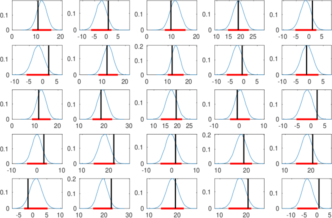
(a) Predictive densities for first 25 locations

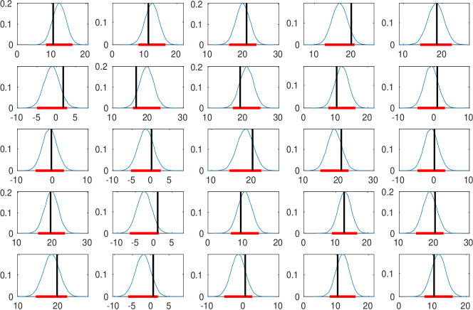
(b) Predictive densities for last 25 locations

Figure 2: Predictive densities of 50 components of the response vector $\mbox{\boldmath{$y$}}_{20}$ corresponding to 50 locations for the data set simulated from mixtures of three GPs. The red horizontal lines denote the 95% predictive intervals. The vertical black lines indicate the true values. All the true values, except one, lie within the 95% predictive intervals. The interval lengths vary from 7.49 to 8.83 units with mean 8.0219 (sd = 0.304879).

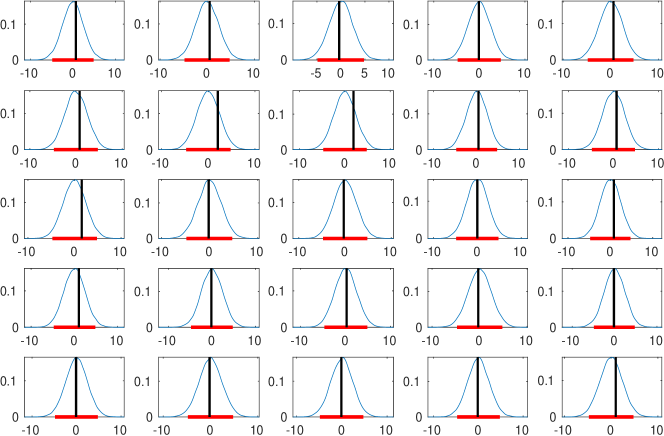
(a) Predictive densities of latent variable for first 25 locations for 3 component mixture of GPs.

(b) Predictive densities of latent variable for last 25 locations for 3 component mixture of GPs.

Figure 3: Predictive densities of 50 components of the latent vector $\mbox{\boldmath{$x$}}_{20}$ corresponding to 50 locations for the data set simulated from mixtures of three GPs. The red horizontal lines denote the 95% predictive interval. The vertical black lines indicate the true values. All the true values lie within the 95% predictive interval. The length of the intervals vary from 9.44 to 9.69 units, with mean 9.55808 (sd = 0.05822192).

6.2 Comparative study with nonstationary GP model

With the data set as generated above, we have fitted the NGP model using the SPDE technique. It is implemented using the package INLA in statistical software R. The posterior predictive densities of $\mbox{\boldmath{$y$}}_{20}$ and $\mbox{\boldmath{$x$}}_{20}$, given $\mathbb{D}$, are provided below for purpose of comparison with the results of our model. It is seen that the 95% predictive intervals of each component of $\mbox{\boldmath{$y$}}_{20}$ contains the true values of $\mbox{\boldmath{$y$}}_{20}$. However, they vary from 1894 to 3364 with mean 2378.483 and standard deviation (sd) = 259.3669 (Figure 4). A similar result is seen for the latent vector $\mbox{\boldmath{$x$}}_{20}$ as well (Figure 5). All the true latent values are contained within the respective 95% predictive intervals, and the range of the length of the 95% intervals is from 1764 to 3053 with mean 2371.798 and standard deviation (sd) = 217.7212 (Figure 5). Clearly, the performance of our model, in terms of the length of predictive intervals for both response $\mbox{\boldmath{$y$}}_{20}$ and latent $\mbox{\boldmath{$x$}}_{20}$ outperformed the NGP model.

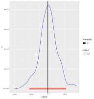
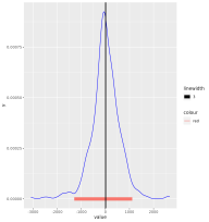
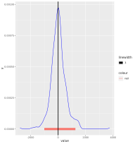
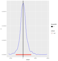
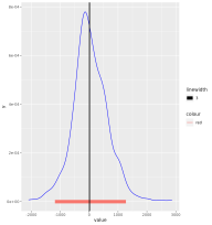
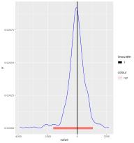
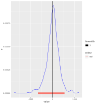
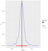
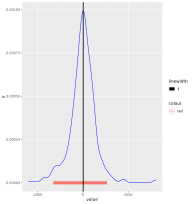
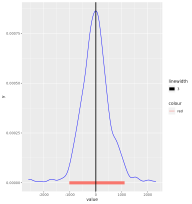
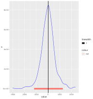
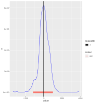
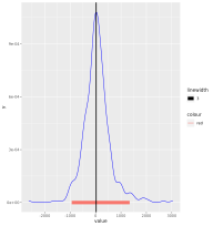
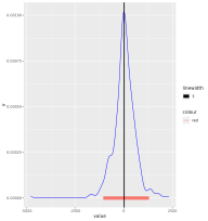
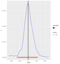
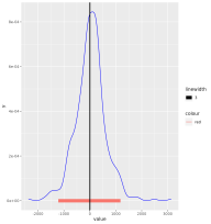
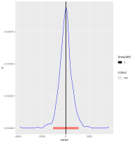
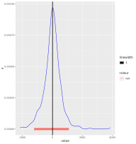
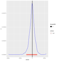
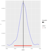
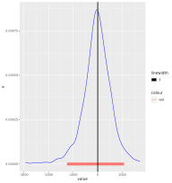
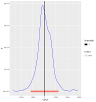
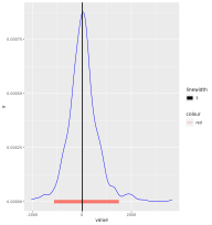
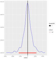
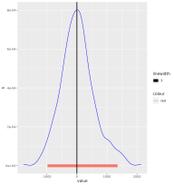
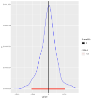
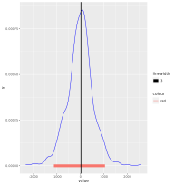
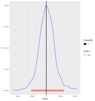
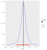
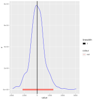
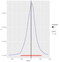
Figure 4: Posterior predictive densities of 50 components of $\mbox{\boldmath{$y$}}_{20}$, corresponding to 50 locations, for data simulated from 3 component mixtures of GPs, using NGP model. The vertical black line indicates the true value and the red horizontal line denotes the 95% predictive intervals. All the true values lie within the 95% predictive intervals. The interval lengths vary from 1894 to 3364 with mean 2378.483 (sd = 259.3669).

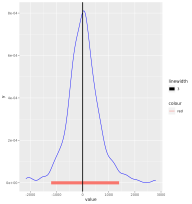
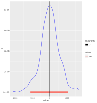
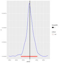
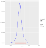
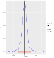
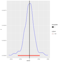
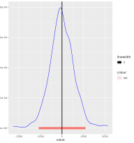
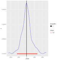
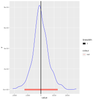
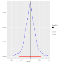
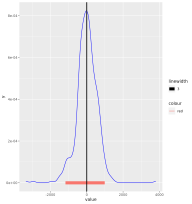
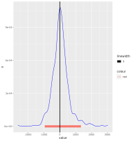
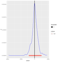
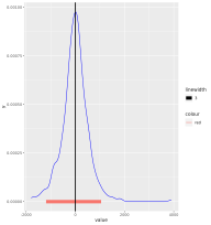
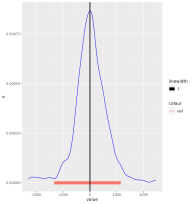
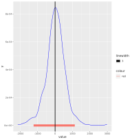
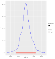
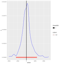
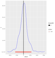
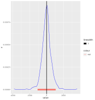
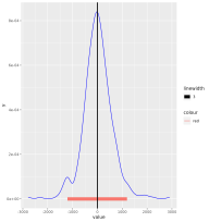
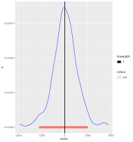
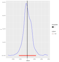
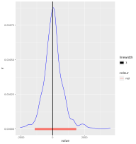
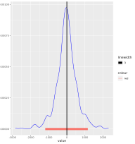
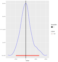
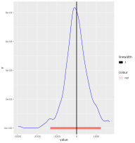
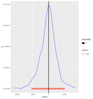
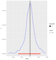
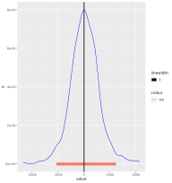
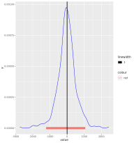
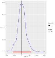
Figure 5: Predictive densities of 50 components of $\mbox{\boldmath{$x$}}_{20}$, corresponding to 50 locations, for data simulated from 3 component mixtures of GPs, using NGP model. The vertical black line indicates the true value and the red horizontal line denotes the 95% predictive intervals. All the true values lie within the 95% predictive intervals. The interval lengths vary from 1764 to 3053 with mean 2371.798 (sd = 217.7212).

6.3 Mixture of two GQNs

For a second comparison study, we choose to simulate from a mixture two highly nonlinear models, called general general quadratic nonlinear (GQN) model. GQN model has widely been used in the literature of spatial and spatio-temporal modeling, see, for example, [55], [45], and [24] for a significant overview of GQN model. We define the GQN model as

$$Y(s_{i},t_{k}) =\phi_{1}(t_{k},s_{i})+\phi_{2}(t_{k},s_{i})\,\tan(X(s_{i},t_{k}))+\epsilon(s_{i},t_{k}),$$ (14)

$$X(s_{i},t_{k}) =\sum_{j=1}^{n}a_{ij}X(s_{j},t_{k-1})+\sum_{j=1}^{n}\sum_{l=1}^{n}b_{ijl}X(s_{j},t_{k-1})[X(s_{l},t_{k-1})]^{2}+\eta(s_{i},t_{k}),$$ (15)

where $i\in\{1,\ldots,n\}$ and $k\in\{1,\ldots,T\}$. The coefficients $\phi_{1}(t_{k},\cdot)$, $\phi_{2}(t_{k},\cdot)$, random errors $\epsilon(t_{k},\cdot)$, $\eta(t_{k},\cdot)$ and the initial latent variable $X(t_{0},\cdot)$ are assumed to be independent, zero-mean Gaussian processes having covariance structure $c(\mbox{\boldmath{$s$}}_{1},\mbox{\boldmath{$s$}}_{2})=\exp\left(-\|\mbox{\boldmath{$s$}}_{1}-\mbox{\boldmath{$s$}}_{2}\|\right)$, for $\mbox{\boldmath{$s$}}_{1},\mbox{\boldmath{$s$}}_{2}\in\mathbb{R}^{2}$, with $\|\cdot\|$ being the Euclidean norm. Moreover, it is assumed that, for $i,j,l\in\{1,\ldots,n\}$, $a_{ij}$ and $b_{ijl}$ have independent univariate 0 mean normal distributions with variance $0.001^{2}$.

6.3.1 Data generation

Here a step by step guidance is provided for generating observations from mixture of two GQNs. Let $n$ and $T$ denote the number of locations and time points.

1. Generate $n$ locations $s_{1},\ldots,s_{n}$ from $[0,1]\times[0,1]$.

2. Generate $n\times T$ matrix $X$ using equation (15) by taking the coefficients as described above.

3. $\mbox{\boldmath{$\phi$}}_{1}(t)$, $\mbox{\boldmath{$\phi$}}_{2}(t)$ and $\mbox{\boldmath{$\epsilon$}}(t)$ are generated independently for $t=1,\ldots,T$ from zero-mean $m-$ variate Gaussian with variance-covariance matrix $\mathbb{S}$, whose $(i,j)$th element is $\exp(-||s_{i}-s_{j}||)$. Let the $i$th element of $\mbox{\boldmath{$\phi$}}_{j}(t)$, $j=1,2$, and $\mbox{\boldmath{$\epsilon$}}(t)$ be $\phi_{j}(t,s_{i})$ and $\epsilon(t,s_{i})$, respectively.

4. Let $u\sim\text{unif}(0,1)$. Given all the parameters and latent variables, generate $Y(s_{i},t)$, for $i=1,\ldots,n$ and $t=1,\ldots,T$, as

   $$Y(s_{i},t)=\begin{cases}\phi_{1}(t,s_{i})+\phi_{2}(t,s_{i})\tan(X(s_{i},t))+\epsilon(t,s_{i})&\text{ if }u<0.6,\\ 5+\phi_{1}(t,s_{i})+\phi_{2}(t,s_{i})\tan(X(s_{i},t))+\epsilon(t,s_{i})&\text{ if }u\geq 0.6.\end{cases}$$

6.3.2 Results from our model

For this data set as well, we run the MCMC iterations for simulating observations from the posterior densities of the parameters involved in our model. These MCMC iterations and Monte Carlo average provide simulated observations from the posterior densities of $\mbox{\boldmath{$y$}}_{20}$ and $\mbox{\boldmath{$x$}}_{20}$, given the data set $\mathbb{D}$. To make the MCMC run feasible one needs to specify the prior parameters. The specific choice of the hyperparameters are mentioned below, except for $\eta_{3}$, which is kept fixed at its MLE 5.5042, obtained by simulated annealing.

6.3.2.1 Choice of prior parameters

Using the same cross-validation technique as before, we obtain the following prior specifications:

$$\alpha^{*}\sim N(0,\sqrt{500}),\beta^{*}\sim N(0,\sqrt{300})$$

$$[\sigma^{2}]\propto IG(780000,2/2),[\sigma^{2}_{\theta}]\propto IG(58900,770/2),[\sigma^{2}_{p}]\propto IG(385,20/2)$$

$$[\eta_{1}^{*}]\propto N(-3,1),[\eta_{2}^{*}]\propto N(-5,1).$$

6.3.2.2 MCMC convergence diagnostics and posterior analysis

The trace plots of the parameters are provided in the Figure S-4, and the posterior density plot of $\mbox{\boldmath{$x$}}_{t},t=1,\ldots,19$ are displayed in Figures S-5 and S-6 of Supplementary Information. The trace plots provide strong evidence of MCMC convergence. Further, the posterior density plots show that the posteriors of the latent variables contain the true latent variable time series at all the 50 locations in the high probability density regions successfully.

The posterior predictive densities of 50 components of $\mbox{\boldmath{$y$}}_{20}$ and $\mbox{\boldmath{$x$}}_{20}$ are provided in Figures 6 and 7, respectively. For the first 25 components of $\mbox{\boldmath{$y$}}_{20}$ Figure  6(a) provides the density plots along with the 95% predictive intervals. They failed to capture true values at three locations, at location $s_{3}$, $s_{8}$ and $s_{13}$, respectively. The posterior predictive densities along with the 95% predictive intervals for the next 25 locations are provided in 6(b). It is seen that all the true values fall within the 95% predictive intervals. Thus, out of 50 locations, except for 3 places, the true response values are captured by the 95% predictive intervals. The lengths of the intervals vary from 99 to 141 units. The mean length of intervals turned out to be 112 with standard deviation (sd) = 7.9680.

In the case of latent vector, $\mbox{\boldmath{$x$}}_{20}$, the posterior predictive density plots of first 25 components of $\mbox{\boldmath{$x$}}_{20}$ are given in 7(a) and that of next 25 components are provided in 7(b). All the true values are captured by the respective predictive intervals. The length of the intervals vary from 138 to 142.5 units with mean 140.4856 and standard deviation (sd) = 0.8524.

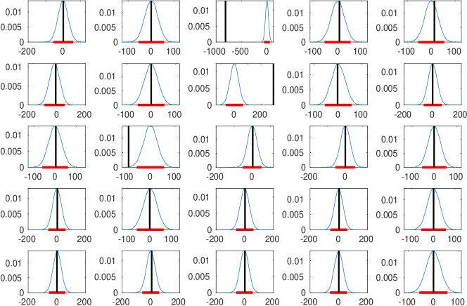
(a) Predictive densities for first 25 locations

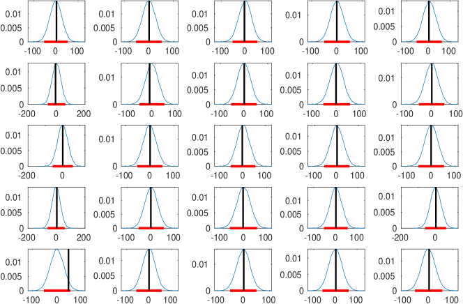
(b) Predictive densities for last 25 locations

Figure 6: Predictive densities of the 50 components of response vector $\mbox{\boldmath{$y$}}_{20}$, corresponding to 50 locations, for data set simulated from mixtures of two GQNs. The red horizontal lines denote the 95% predictive intervals. The vertical black lines indicate the true values. All the true values, except three, lie within the 95% predictive intervals. The interval lengths vary from 99 to 141 units, with mean 112.9458 (sd = 7.9680).

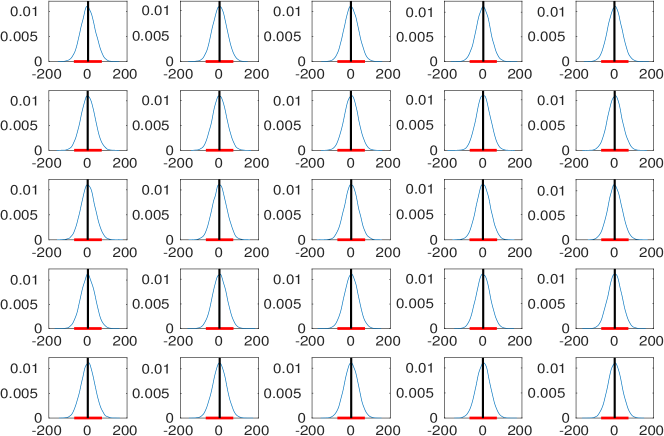
(a) Predictive densities of latent variable for first 25 locations.

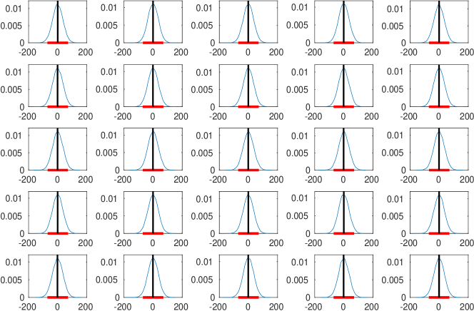
(b) Predictive densities of latent variable for last 25 locations.

Figure 7: Predictive densities of the 50 components of latent vector $\mbox{\boldmath{$x$}}_{20}$, corresponding to 50 locations, for data set simulated from mixtures of two GQNs. The red horizontal lines denote the 95% predictive interval. The vertical black lines indicate the true values. All the true values lie within the 95% predictive interval. The length of the intervals vary from 138 to 142.5 units with mean 140.4856 (sd = 0.8524).

6.3.3 Comparative study with nonstationary GP model

Similar to the analysis of mixture of GP models, we fitted the NGP model on the current data set using INLA in R. For the purpose of fitting the NGP model, the same SPDE technique has been implemented. The posterior predictive densities for the components of $\mbox{\boldmath{$y$}}_{20}$ and $\mbox{\boldmath{$x$}}_{20}$ are reported in Figures 8 and 9, respectively. The 95% predictive intervals of the components of $\mbox{\boldmath{$y$}}_{20}$ capture the true values except for 3rd, 8th and 12th components. The range of the lengths of the predictive intervals is from 172 to 233.5 units. The mean length of the intervals turned out to be 200.79 with standard deviation (sd) = 10.1872. Therefore, the mean length of the predictive intervals is more than 1.75 times the mean length of the predictive intervals our proposed model. It is interesting to see that none of the true values were captured by the 95% predictive intervals of the posterior predictive densities of the components of $\mbox{\boldmath{$x$}}_{20}$ (Figure 9). Surprisingly, the lengths of the intervals turned out to be too small, in the order of $10^{-4}$. Hence from the analysis of this simulated data set, we observe that the performance of our model is significantly better than that of the NGP model for the mixture of GQN data set.

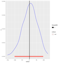
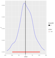
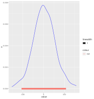
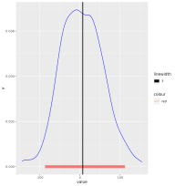
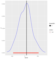
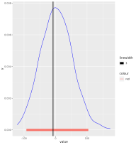
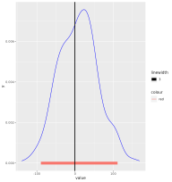
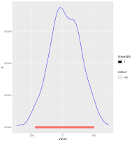
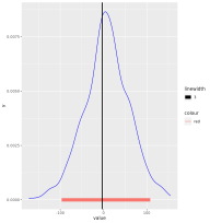
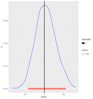
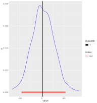
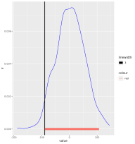
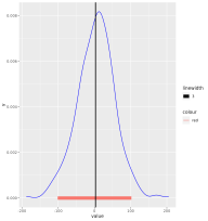
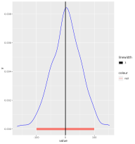
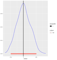
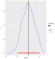
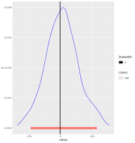
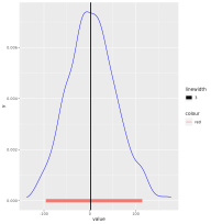
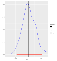
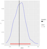
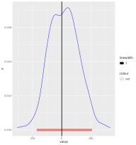
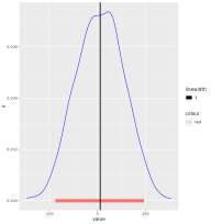
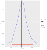
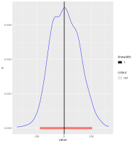
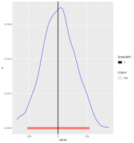
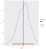
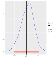
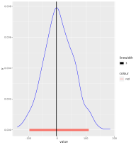
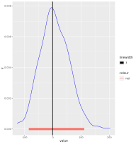
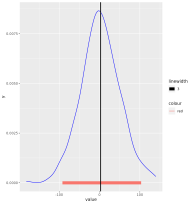
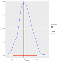
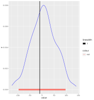
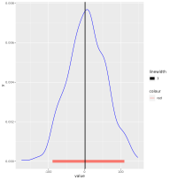
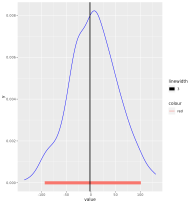
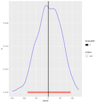
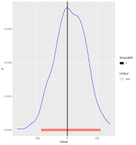
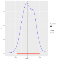
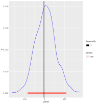
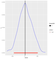
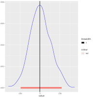
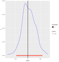
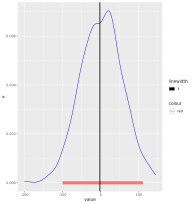
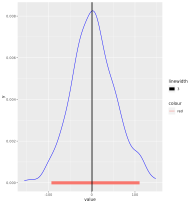
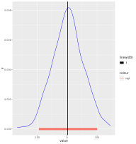
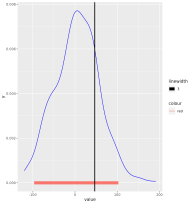
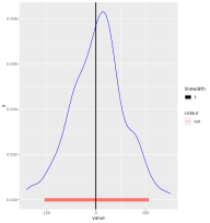
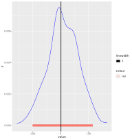
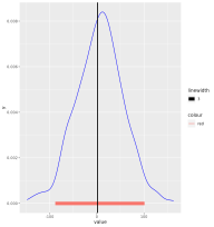
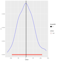
Figure 8: Predictive densities of 50 components of response vector $\mbox{\boldmath{$y$}}_{20}$, corresponding to 50 locations, for data simulated from mixtures of two GQNs, using NGP model. The vertical black line indicates the true value and the red horizontal line denotes the 95% predictive intervals. All the true values lie within the 95% predictive intervals. The interval lengths vary from 172 to 233.5 with mean 200.79 (sd = 10.18972).

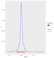
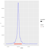
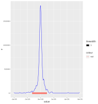
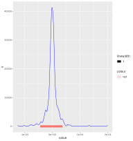
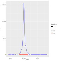
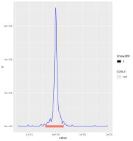
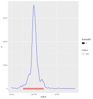
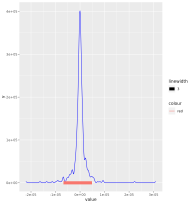
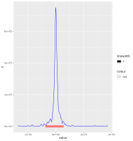
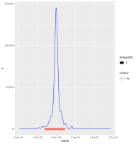
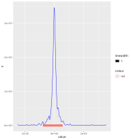
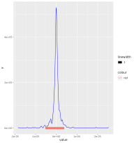
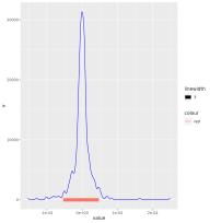
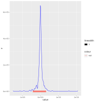
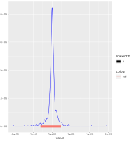
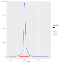
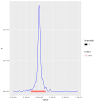
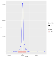
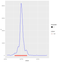
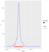
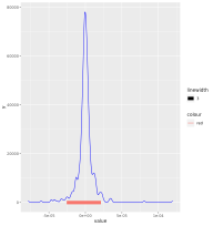
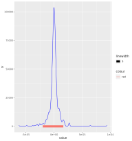
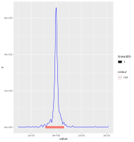
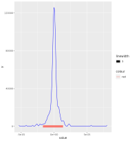
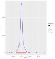
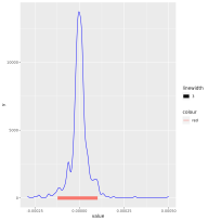
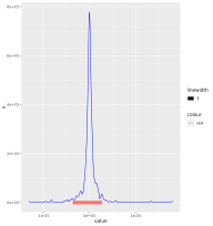
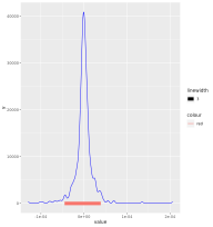
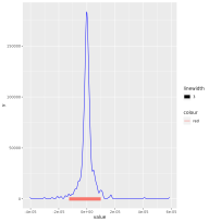
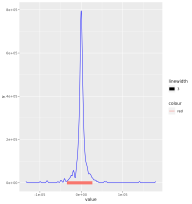
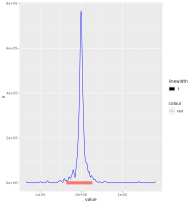
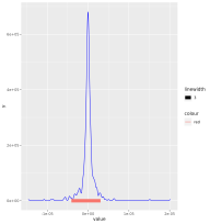
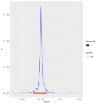
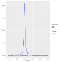
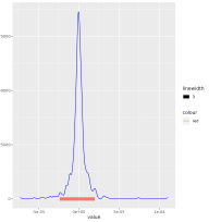
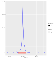
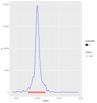
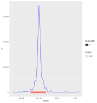
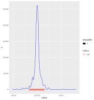
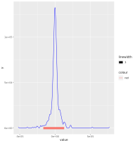
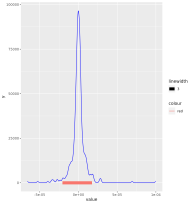
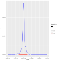
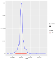
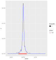
Figure 9: Predictive densities of 50 components of latent vector $\mbox{\boldmath{$x$}}_{20}$, corresponding to 50 locations, for data simulated from mixtures of two GQNs, using NGP model. The red horizontal line denotes the 95% predictive intervals. None of the true values lie within the respective predictive interval. The interval lengths are of the order $10^{-4}$.

7 Real data analysis

We evaluate our model performance on two real data sets on temperatures. The first spatio-temporal data is the temperature values taken around Alaska recorded for 65-70 years. The second data set consists of sea surface temperatures over a wide range of areas, recorded for 100 months. The details of the data sets are provided in Sections 7.1 and 7.2, respectively.

Before applying our model on these data sets, we first make the following transformation (Lambert projection, see [46]) of the locations so that the Euclidean distance make more sense. Let $\phi$ be longitude and $\psi$ be latitude in radian. Then the following transformation is made:

$$s_{1} =2\sin\left(\frac{\pi}{4}-\frac{\psi}{2}\right)\sin\phi;$$

$$s_{2} =-2\sin\left(\frac{\pi}{4}-\frac{\psi}{2}\right)\cos\phi.$$

7.1 Alaska temperature data

A real data analysis is done on the temperature data of Alaska and its surroundings. The data set is collected from https://www.metoffice.gov.uk/hadobs/crutem4/data/download.html by clicking the link CRUTEM.4.6.0.0.station_files.zip given under the heading Station data. The details of the data set can be read from https://crudata.uea.ac.uk/cru/data/temperature/crutem4/station-data.htm.

A total of 30 locations are considered for the analysis. Annual average temperature data for the years 1950 to 2015 are taken after detrending. Of these 30 locations, at four locations many data were missing. So, we decided to construct the complete time series for these four locations. Among these 30 locations, data till 2021 were available for 16 positions. We thus have made multiple time predictions for these 16 locations. The 26 spatial points are indicated in Figure 10 in red and 4 locations (for which the complete time series is reconstructed) are indicted in blue in the same graph. The latitudes and longitudes are provided in Table 1.

Sl No.	1	2	3	4	5	6	7	8	9	10	11	12	13	14	15
Latitude	71.3N	60.6N	59.5N	55.2N	61.2N	70.1N	64.5N	66.9N	59.6N	60.5N	64.8N	60.1N	63N	63N	55N
Longitude	156.8W	151.3W	139.7W	162.7W	150W	143.6W	165.4W	151.5W	151.5W	145.5W	147.9W	149.5W	155.6W	141.9W	131.6W
Sl No.	16	17	18	19	20	21	22	23	24	25	26	27	28	29	30
Latitude	61.6N	64N	60.8N	57.8N	58.7N	62.2N	66.9N	58.4N	63.7N	68.2N	59.6N	62.8N	64.1N	67.4N	60.7N
Longitude	149.3W	145.7W	161.8W	152.5W	156.7W	145.5W	162.6W	134.6W	149W	135W	133.7W	137.4W	139.1W	134.9W	135.1W

Table 1: Latitude and Longitude (in degrees) of 30 locations in and around Alaska. The locations corresponding to the serial numbers, indicated in bold, are used for multiple predictions. The serial numbers which are denoted in blue, for the corresponding spatial locations, complete time series are reconstructed. These blue serial numbers are indicated by $L_{25},L_{26},L_{28}$ and $L_{30}$ for future references.

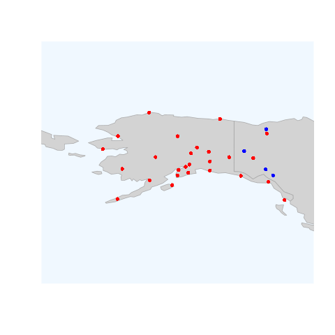
Figure 10: The map of Alaska and its surroundings. The red dots indicate the locations at which the data for the year 1950-2015 are considered. The positions indicated by blue dots at which the spatial prediction are made for the complete time series.

Thus the data set considered here contains 26 locations and 65 time points from 1950 to 2014 (last time point is set aside for the purpose of single time point prediction). We denote the data set by $\mathbb{D}=\{\mbox{\boldmath{$y$}}_{1},\ldots,\mbox{\boldmath{$y$}}_{65}\}$, where $\mbox{\boldmath{$y$}}_{t}$, $t\in\{1,\ldots,65\}$, is a 26 dimensional vector. In this analysis, we have made both temporal and spatial predictions after detrending the data. At these 26 locations, we obtained the predictive densities for the year 2015 and for 16 locations (indicated by $L_{1},\ldots,L_{7}$, $L_{11}\ldots,L_{13}$, $L_{18},\ldots,L_{20}$, $L_{22}$, $L_{27}$, $L_{29}$ for references hereafter) we made multiple time point predictions. Along with these temporal predictions, we constructed the 95% predictive intervals for the complete time series for the 4 left out locations. To do this, we augmented the data set $\mathbb{D}$ with the initial values for the 65 time points of the four locations and then updated the values by calculating the conditional densities given the data set $\mathbb{D}$. That is to say, we start with $\mathbb{D}^{*}=\{\mbox{\boldmath{$y$}}_{1}^{*},\ldots,\mbox{\boldmath{$y$}}_{65}^{*}\}$, where $\mbox{\boldmath{$y$}}_{t}^{*}$ is a 30 dimensional vector, with the last four values augmented with $\mbox{\boldmath{$y$}}_{t}$, for $t\in\{1,\ldots,65\}$. The parameters of our model, including the latent variables, are updated given $\mathbb{D}^{*}$, and then the last four values of $\mbox{\boldmath{$y$}}^{*}_{t}$ are updated given the parameter values and latent variables. This is continued for the complete MCMC run.

In Section S-9 of Supplementary Information, we validate that the underlying spatio-temporal process that generated the Alaska data is non-Gaussian, strictly stationary, and the lagged correlations converge to zero as the lags tend to infinity. Besides, there is no reason to assume separability of the spatio-temporal covariance structure. Although our spatio-temporal process is nonstationary, it is endowed with the other desirable features, and the results of analysis of the Alaska data show that it is an appropriate model for this data.

7.1.1 Prior choices for the Alaska temperature data

With the same cross-validation technique as in the simulation experiments, the complete specifications of the priors are obtained as follows:

$$\alpha^{*}\sim N(0,\sqrt{500}),\beta^{*}\sim N(0,\sqrt{300}),$$

$$[\sigma^{2}]\propto IG(450000,2/2),[\sigma^{2}_{\theta}]\propto IG(700,780/2),[\sigma^{2}_{p}]\propto IG(250,100/2),$$

$$[\eta_{1}^{*}]\propto N(-3,1),[\eta_{2}^{*}]\propto N(-5,1).$$

As before, we fix $\eta_{3}$ at its maximum likelihood estimate 5.0581.

7.1.2 Results of the Alaska temperature data

As for the case of the simulation studies, we implemented 1,75,000 MCMC iterations with the first 1,50,000 iterations as burn-in. The time taken was about 5 hours 43 minutes in our desktop computer. The MCMC trace plots for the parameters, except $\eta_{3}$, are given in Figure S-7 of Supplementary Information, which bear clear evidence of convergence in each case. The posterior densities of the latent variables are displayed in Figure S-8 of Supplementary Information.

The predictive densities for $\mbox{\boldmath{$y$}}_{66}$ for 26 locations are depicted in Figure 11. All the true values (detrended temperature values), which are denoted by black bold vertical lines, lie well within the 95% predictive intervals (indicated as red bold horizontal lines in the figures). The predictive densities for the years 2016-2021 at the 16 locations are shown in two figures (Figure 12 and Figure 13), each containing 8 locations. Except for one location, at one time point, in all the other scenarios, the true values are captured by the 95% predictive intervals associated with our model.

The complete time series for the four locations, which were indicated in blue in Figure 10, are reconstructed using our model. The Bayesian predictive densities at each time point for these locations are shown in Figure 14 using probability plot. Higher the intensity of the color, higher is the density. The available true detrended temperature values at these locations are plotted and depicted by black stars in Figure 14. At one location ($L_{30}$), three values lie away from the high density region. However, from the pattern of the data values, it seems that these values are outlying in comparison to the rest of the values. Other than these, all the available true detrended temperatures lie within high density regions (except one value at $L_{28}$). In a nutshell, we can claim that our model performs well in analyzing the temperature data of Alaska and its surroundings.

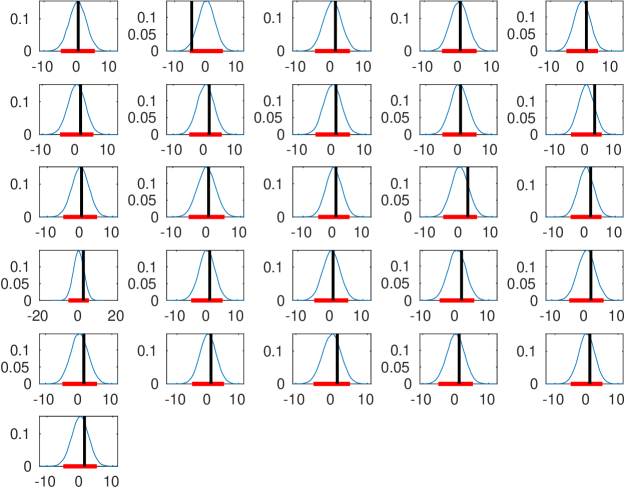
Figure 11: Posterior predictive densities of the detrended temperatures for the year 2015 at 26 locations for the Alaska temperature data. The red horizontal lines denote the 95% predictive intervals. The vertical black lines indicate the true values. All the true values lie within the 95% posterior predictive intervals.

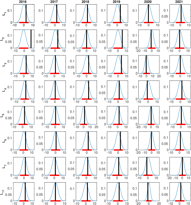
Figure 12: Predictive densities of the detrended temperatures for the years 2016-2021 at 8 locations for the Alaska temperature data. The eight locations are indicated by $L_{1}\,\ldots,L_{7}$, and $L_{11}$ at the left side of the figure corresponding to the rows. The years are shown at the top of the figure corresponding to the columns. The red horizontal line in each plot denotes the 95% posterior predictive interval. The vertical black lines indicate the true values. All the true values, except one, lie within the 95% posterior predictive intervals.

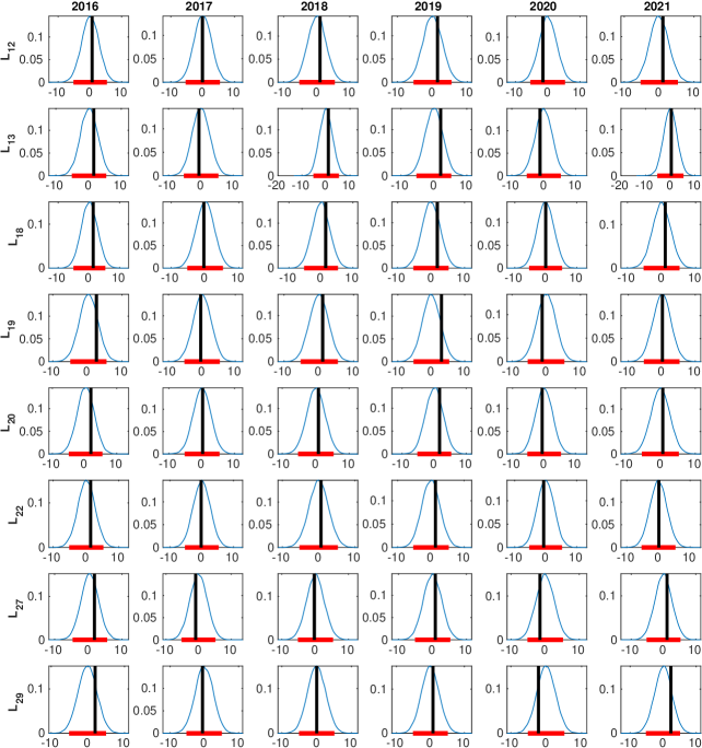
Figure 13: Predictive densities of the detrended temperatures for the years 2016-2021 at other 8 locations for the Alaska temperature data. The eight locations are indicated by $L_{12}$, $L_{13}$, $L_{18},L_{19},L_{20}$, $L_{22}$, $L_{27}$ and $L_{29}$ at the left side of the figure corresponding to the rows. The years are shown at the top of the figure corresponding to the columns. The red horizontal line in each plot denotes the 95% posterior predictive interval. The vertical black lines indicate the true values. All the true values lie within the 95% posterior predictive interval.

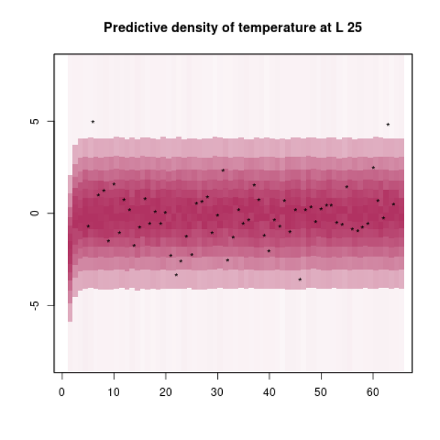
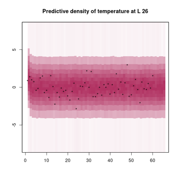
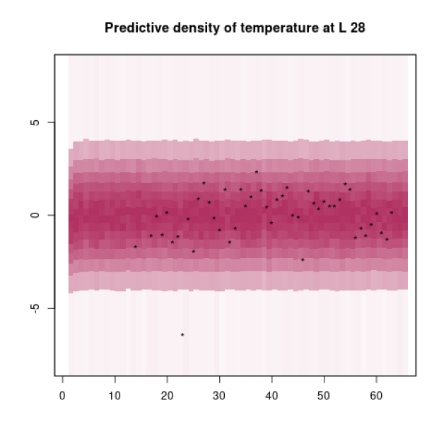
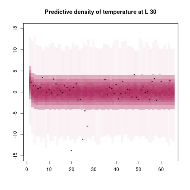
Figure 14: Posterior predictive densities of the reconstructed detrended temperature data of Alaska and its surroundings at 8 locations. Higher the intensity of the colour, higher is the probability density. The black stars represent the available true temperature values (detrended). Except for 3 to 4 points at $L_{30}$, and one point at $L_{28}$, all the other points fall within the high probability density region.

7.2 Sea surface temperature data

The sea surface temperature data is obtained from http://iridl.ldeo.columbia.edu/SOURCES/.CAC/. For the purpose of illustration, we have taken spatio-temporal observations of the first 40 locations and the first 100 time points from the complete data set. The locations of the chosen data set varies from 56^∘W to 110^∘E and 19^∘S to 25^∘N. The locations are given in Table 2. Hundred monthly average temperatures are taken starting from the month of January 1970. Among these 40 locations and 100 time points, observations corresponding to 30 locations and 99 time points are taken as the learning set. The observations corresponding to the last 10 locations and the last time point are kept aside for the prediction purpose. Only for the sake of convenience, the time series at each location is referenced to its mean, in the sense that the mean of the time series at each location is subtracted from the original data.

Sl No.	1	2	3	4	5	6	7	8	9	10
Latitude	19S	19N	19S	17N	7N	11S	3S	25S	25N	7N
Longitude	108E	20W	42E	58E	2W	76E	2E	28W	100E	26W
Sl No.	11	12	13	14	15	16	17	18	19	20
Latitude	1N	19S	13N	27N	5S	17S	7S	23S	21S	1S
Longitude	84E	14E	48E	18W	110E	46W	10W	14E	36W	28W
Sl No.	21	22	23	24	25	26	27	28	29	30
Latitude	13N	7S	29N	15S	1N	1S	13S	9N	15N	25S
Longitude	30E	36E	104E	24W	72E	46W	64E	12E	24E	52E
Sl No.	31	32	33	34	35	36	37	38	39	40
Latitude	25N	7N	11N	5N	7N	19S	1S	17S	19S	29N
Longitude	4E	52E	18E	16W	56W	106E	20W	28W	0	48W

Table 2: Latitude and Longitude (in degrees) of 40 locations for the sea surface temperature data. The locations corresponding to the serial numbers, indicated in bold, are used for complete time series prediction. These bold serial numbers are indicated as $L_{31},\ldots,L_{40}$ for the future reference.

As in the Alaska temperature data analysis, we denote the learning data set by $\mathbb{D}=\{\mbox{\boldmath{$y$}}_{1},\ldots,\mbox{\boldmath{$y$}}_{99}\}$, where $\mbox{\boldmath{$y$}}_{t}$ is a 30 dimensional spatial observation at time point $t$. At these 30 locations, we obtain the posterior predictive densities for the 100th time point and find out the high probability density regions for the entire time series of the locations corresponding to the serial numbers indicated in bold within Table 2. These locations are referred to as $L_{31},\ldots,L_{40}$ hereafter. For calculating the posterior predictive densities at 99 time points for the above mentioned 10 spatial locations, the data set $\mathbb{D}$ is first augmented with the initial values for 99 time points of the ten locations and then the values are updated by sampling from the corresponding conditional distributions given the data set $\mathbb{D}$. That is to say, we start with $\mathbb{D}^{*}=\{\mbox{\boldmath{$y$}}_{1}^{*},\ldots,\mbox{\boldmath{$y$}}_{99}^{*}\}$, where $\mbox{\boldmath{$y$}}_{t}^{*}=[\mbox{\boldmath{$y$}}_{t}^{T}:\mbox{\boldmath{$z$}}_{t}^{T}]^{T}$ is a 40 dimensional vector, with $\mbox{\boldmath{$z$}}_{t}$ being the initial guess for the ten locations $L_{31},\ldots,L_{40}$, $t\in\{1,\ldots,99\}$. The parameters of our model, including the latent variables, are then updated given $\mathbb{D}^{*}$, and then the last ten values of $\mbox{\boldmath{$y$}}^{*}_{t}$ are updated given the parameter values and the latent values. This continues for the entire MCMC run. Note that this sea surface temperature data arises from a nonstationary (both weakly and strongly), non-Gaussian spatio-temporal process with lagged correlations tending to zero (refer to [24] for further details).

7.2.1 Prior choices for sea surface temperature data

Following our cross-validation technique to obtain the hyper parameters, we completely specify the priors as follows:

$$\alpha^{*}\sim N(0,\sqrt{500}),\beta^{*}\sim N(0,\sqrt{300}),$$

$$[\sigma^{2}]\propto IG(35000,2/2),[\sigma^{2}_{\theta}]\propto IG(1000,780/2),[\sigma^{2}_{p}]\propto IG(90,100/2)$$

$$[\eta_{1}^{*}]\propto N(-3,1),[\eta_{2}^{*}]\propto N(-5,1).$$

As before, we fixed $\eta_{3}$ at its maximum likelihood estimate; here the value is 14.2981.

7.2.2 Controlling $M_{s}$

Since the locations are distributed very widely over the space, the value of $M_{s}$ becomes too large for this data for a given $s$. Now $M_{s}$ appears in the denominator of the variance covariance matrix of the predictive densities of the time series at a particular location (see equation (3.1)). Therefore, the variability becomes too less. So, to control the variability we modify the definition of $M_{s}$ as $M_{s}=\exp(c\,\max\{||s^{2}-u^{2}||^{2}:u\in S\})$, where $c$ is a positive small constant. Note that it does not hamper the properties of $M_{s}$ and hence all the theoretical properties of the processes remain unchanged. The constant $c$ controls the spatial variability which can be thought of as a distance scaling factor. The choice of $c$ was also done by cross-validation. It was found that $c=0.25$ works reasonably well for the sea surface temperature data.

7.2.3 Results of the sea surface temperature data

Figure S-9 of Supporting Information, representing the MCMC trace plots of the parameters, exhibits no evidence of non-convergence of our MCMC algorithm. The posterior predictive colour density plots for the latent variables are shown in Figure S-10 of Supporting Information.

Next we provide the posterior predictive densities at the 100th month for each of the 30 locations. Thirty density plots are shown in Figure 15. As the plots indicate, the posterior predictive densities for the future time point correctly contains the true values for all of these locations. The results encourage us to use the proposed model for the future time point prediction for a nonstationary spatio-temporal data.

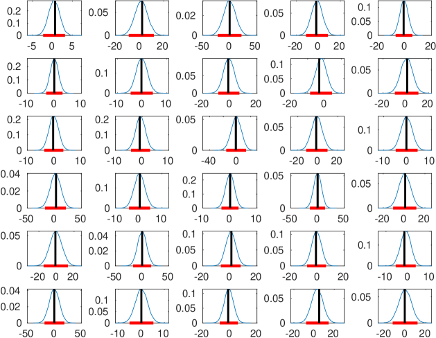
Figure 15: Predictive densities of averaged referenced temperatures for the 100th month at 30 locations for the sea surface temperature data. The red horizontal lines denote the 95% predictive interval. The vertical black lines indicate the true values. All the true values lie within the 95% predictive interval.

Another important aspect of the spatio-temporal modeling is to predict the complete time series at the given locations. As mentioned in Section 7.2, we kept aside the complete temporal observations for the ten locations for evaluating the performance of the proposed model. As described in Section 7.2, we obtained the posterior predictive densities for each of the 99 time points for a given location. The plots are depicted in Figure 16. As one can see, except for the two locations, which are represented by $L_{36}$ and $L_{39}$, most of the true values, indicated by black stars in Figure 16, fall well within the high probability density regions. Next, we give a plausible explanation for the poor performance at the locations $L_{36}$ and $L_{39}$.

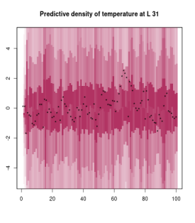
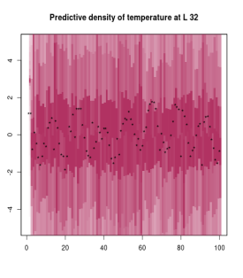
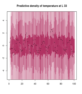
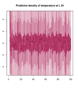
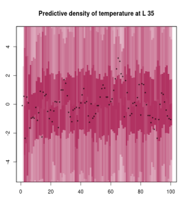
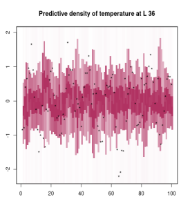
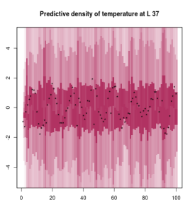
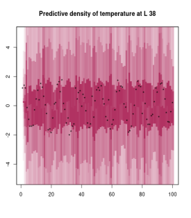
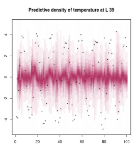
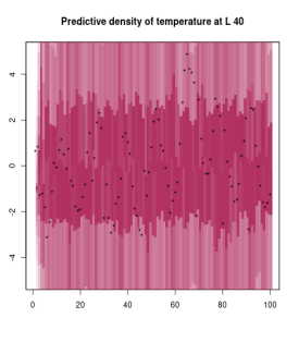
Figure 16: Posterior predictive densities of the reconstructed time series of sea surface temperature data (average referenced) at ten locations. Higher the intensity of the colour, higher is the probability density. The black stars represents the true temperature values (average referenced). Except for the locations denoted by $L_{36}$ and $L_{39}$, majority of the true values fall well within the high density regions.

7.2.4 Plausible explaination for the poor performance at the two locations

First we provide below a plot (Figure 17) which represents the locations of the sea temperature data after we make the Lambert projections (see equation (7)). The blue dots in Figure 17 are used as the test set locations for the complete time series prediction. Two points are specially indicated by a black star and a green star. These two locations are also members of the test set and at these two locations the high probability density regions fail to capture majority of the true values. The black star corresponds to $L_{36}$ and the green star corresponds to $L_{39}$.

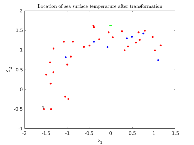
Figure 17: Locations of sea surface temperature data after the transformation given in equations 7. The red points represent the locations of the observations in the learning set. The blue solid dots, the black and the green stars are the locations of the observations in the test set.

From the above plot, it is evident that the location which is indicated by black star, that is, $L_{36}$, is far away from the majority of the other locations. Thus, the value of $M_{s}$ for location $L_{36}$ becomes too large making the variability of the predictive densities for every time point very small. For this reason, the high posterior density region could not capture the true value well as compared to other locations (except $L_{39}$). On the other hand, the location indicated by green star is not far apart from the rest of the locations. However, the variability of the observations obtained across the time points are comparatively very large than the variability of the observations at other points. In fact, the variability across the time points of $L_{39}$ is found to be 8.4670 which is more than double the variability of all other locations present in the test set. In addition, at $L_{39}$ more than 70% data lie away from -2 and 2, while the mean remains close to 0. This makes $L_{39}$ unique among the other test locations. Furthermore, it is observed that the mean variability of the learning set locations is 2.0407 and more than 90% locations have data variability less than 5.3314. Therefore, from the learning data, the model did not get enough training to deal with such highly variable data. These are the reasons why the proposed model could not perform as expected for these two particular locations.

To end this discussion, we note that even when location $L_{36}$ is far away from the rest, thanks to our modification of $M_{s}$, the model performs better at this location than at location $L_{39}$. The large temporal variability compared to other locations including training and test sets, made this point ($L_{39}$) an outlier and that is why the predictive densities failed to capture the true values.

8 Summary and conclusion

Although Hamiltonian equations are very well-known in physics, in statistics its importance is confined to Hamiltonian Monte Carlo for simulating approximately from posterior distributions. However, given the success of the Hamiltonian equations in phase-space modeling, it is not difficult to anticipate its usefulness in spatio-temporal statistics, if properly exploited. This key insight motivated us to build a new spatio-temporal model through the leap-frog algorithm of a suitably modified set of Hamiltonian equations, where stochasticity is induced through appropriate Gaussian processes. Our marginal, observed stochastic process is nonparametric, non-Gaussian, nonstationary, nonseparable, with appropriate dynamic temporal structure, with time treated as continuous. Additionally, the lagged correlations between the observations tend to zero as the space-time lag goes to infinity. Hence, compared to the existing spatio-temporal processes, our process seems to be the most realistic. Indeed, our simulation experiments reveal that for general spatio-temporal datasets, our model very significantly outperforms the popular approach of latent process spatio-temporal modeling based on nonstationary Gaussian processes. Furthermoe, suitability and flexibility of our model is vindicated by the results of our applications to two real data sets. Interesting continuity and smoothness properties add further elegance to our new process.

We did not try to analyse particularly sizable datasets in this article. In our future endeavors, we shall consider application of our ideas to very big datasets using basis representation and a variable dimensional MCMC techniques called TTMCMC, which was proposed by [56].

Acknowledment

We are thankful to Dr. Moumita Das for her insightful comments, which greatly enhanced the presentation quality of our manuscript.

Supplemental Material

S-1 Proofs of the theorems

Lemma S-1.1

$M_{s}$ is infinitely differentiable in $s\in S$.

Proof: Since the exponential function is infinitely differentiable, it is sufficient to show that $\max\{||s^{2}-u^{2}||^{2}:u\in S\}$ is infinitely differentiable with respect to $s$. We first prove the result in one dimension and then will generalize to higher dimension. Let $S$ be a compact set in $\mathbb{R}$. We consider different cases as follows.

Case 1: Let $S=[a,b]$, where $0<a<b$. Then $\max\{|s^{2}-u^{2}|^{2}:u\in[a,b]\}=s^{4}+\max(a^{4},b^{4})-2s^{2}a^{2}$, which is an infinitely smooth function of $s$.

Case2: Let $S=[a,b]$, where $a<b<0$. Then $\max\{|s^{2}-u^{2}|^{2}:u\in[a,b]\}=s^{4}+\max(a^{4},b^{4})-2s^{2}b^{2}$, which is also infinitely differentiable function of $s$.

Case 3: Let $S=[-a,b]$, where $a,b>0$. Then

$$\max\{|s^{2}-u^{2}|^{2}:u\in[-a,b]\}=s^{4}+\max(a^{4},b^{4})-2s^{2}\min(a^{2},b^{2})$$ (1)

Clearly, $\max\{|s^{2}-u^{2}|^{2}:u\in[-a,b]\}$ is infinitely differentiable function of $s$, for any $s\in[-a,b]$.

Now suppose that $S=[-a_{1},b_{1}]\times[-a_{2},b_{2}]$, where $a_{i},b_{i}$ are positive for each $i=1,2$. Let $s\in S$. Define $f_{s}:S\rightarrow\mathbb{R}$, such that $f_{s}(u)=||s^{2}-u^{2}||^{2}=(s_{1}^{2}-u_{1}^{2})^{2}+(s_{2}^{2}-u_{2}^{2})^{2}$. Define $f_{1s}(u_{1})=(s_{1}^{2}-u_{1}^{2})^{2}$ and $f_{2s}(u_{2})=(s_{2}^{2}-u_{2}^{2})^{2}$. Therefore, $f_{s}(u)=f_{1s}(u_{1})+f_{2s}(u_{2})$ and $\max\limits_{u\in S}f_{s}(u)=\max\limits_{u\in S}[f_{1s}(u_{1})+f_{2s}(u_{2})]=\max\limits_{u_{1}\in[-a_{1},b_{1}]}f_{1s}(u_{1})+\max\limits_{u\in[-a_{2},b_{2}]}f_{2s}(u_{2})$. The equality follows as $u=(u_{1},u_{2})\in S,$ with $u_{1}\in[-a_{1},b_{1}]$ and $u_{2}\in[-a_{2},b_{2}]$. We have already proved that (Case 3, equation (1)) $\max\limits_{u_{i}\in[-a_{i},b_{i}]}f_{is}(u_{i})=s_{i}^{4}+\max(a_{i}^{4},b_{i}^{4})-2s_{i}^{2}\min(a_{i}^{2},b_{i}^{2})$ for $i=1,2$. Hence $\max\limits_{u\in S}f_{s}(u)=\sum\limits_{i=1}^{2}s_{i}^{4}+\max(a_{i}^{4},b_{i}^{4})-2s_{i}^{2}\min(a_{i}^{2},b_{i}^{2})$, which is infinitely differentiable with respect to $s_{1}$ and $s_{2}$.

If $S=[a_{1},b_{1}]\times[a_{2},b_{2}]$ where (i) $0<a_{1}<b_{1}$ and $0<a_{2}<b_{2}$ or (ii) $a_{1}<b_{1}<0$ and $a_{2}<b_{2}<0$ or (iii) $0<a_{1}<b_{1}$ and $a_{2}<b_{2}<0$ or (iv) $a_{1}<b_{1}<0$ and $0<a_{2}<b_{2}$, the proof goes in a similar manner as above except that now we have to use Case 1 and Case 2 for one dimension, instead of Case 3. $\square$

Theorem S-1.1

Under assumptions A1 to A3, cov$\left(Y(s,h\delta t),Y(s^{\prime}h^{\prime}\delta t)\bigg{|}X\right)$ converges to 0 as $||s-s^{\prime}||\rightarrow\infty$ and/or $|h-h^{\prime}|\rightarrow\infty$.

Proof: Let us denote $Y(s,\cdot)$ as $\theta_{s}(\cdot)$, $Y(s^{\prime},\cdot)$ as $\theta_{s^{\prime}}(\cdot)$ and $X$ by $p$. Without loss of generality let us assume that $h>h^{\prime}$. Now

$$\mbox{cov}\left(\theta_{s}(h\delta t),\theta_{s^{\prime}}(h^{\prime}\delta t)\Big{|}p\right)$$

$$\quad=\mbox{cov}\left(\beta\theta_{s}((h-1)\delta t)+\frac{\delta t}{M_{s}}\left\{\alpha p_{s}((h-1)\delta t)-\frac{\delta t}{2}\frac{\partial}{\partial\theta_{s}}V\left(\theta_{s}((h-1)\delta t)\right)\right\},\theta_{s^{\prime}}(h^{\prime}\delta t)\Big{|}p\right)$$

$$\quad=\mbox{cov}(\beta\theta_{s}((h-1)\delta t),\theta_{s^{\prime}}(h^{\prime}\delta t)\Big{|}p)-\frac{1}{2}\frac{(\delta t)^{2}}{M_{s}}\mbox{cov}\left(\frac{\partial}{\partial\theta_{s}}V(\theta_{s}((h-1)\delta t)),\theta_{s^{\prime}}(h^{\prime}\delta t)\Big{|}p\right)$$

$$\quad=\cdots$$

$$\quad=\beta^{h-h^{\prime}}\mbox{cov}\left(\theta_{s}(h^{\prime}\delta t),\theta_{s^{\prime}}(h^{\prime}\delta t)|p\right)-\frac{1}{2}\frac{(\delta t)^{2}}{M_{s}}\sum_{k=1}^{h-h^{\prime}}\beta^{k-1}\mbox{cov}\left[\frac{\partial}{\partial\theta_{s}}V\left(\theta_{s}((h-k)\delta t)\right),\theta_{s^{\prime}}(h^{\prime}\delta t)|p\right].$$ (2)

Since, for any $1\leq\ell\leq h-h^{\prime}$,

$$\mbox{cov}\left(\frac{\partial}{\partial\theta_{s}}V\left(\theta_{s}((h-\ell)\delta t)\right),\theta_{s^{\prime}}(h^{\prime}\delta t)\Big{|}p\right)$$

$$\quad=\mbox{cov}\left(\frac{\partial}{\partial\theta_{s}}V\left(\theta_{s}((h-\ell)\delta t)\right),\beta\theta_{s^{\prime}}((h^{\prime}-1)\delta t)+\frac{\delta t}{M_{s^{\prime}}}\left\{\alpha p_{s}((h^{\prime}-1)\delta t)-\frac{\delta t}{2}\frac{\partial}{\partial\theta_{s^{\prime}}}V\left(\theta_{s}((h^{\prime}-1)\delta t)\right)\right\}\Big{|}p\right)$$

$$\quad=\beta\mbox{cov}\left(\frac{\partial}{\partial\theta_{s}}V\left(\theta_{s}((h-\ell)\delta t)\right),\theta_{s^{\prime}}((h^{\prime}-1)\delta t)\Big{|}p\right)-\frac{(\delta t)^{2}}{2M_{s^{\prime}}}\mbox{cov}\left(\frac{\partial}{\partial\theta_{s}}V\left(\theta_{s}((h-\ell)\delta t)\right),\frac{\partial}{\partial\theta_{s^{\prime}}}\right.$$

$$\qquad\left.V\left(\theta_{s^{\prime}}((h-1)\delta t)\right)\Big{|}p\right)$$

$$\quad=\cdots$$

$$\quad=\beta^{h^{\prime}}\mbox{cov}\left(\frac{\partial}{\partial\theta_{s}}V\left(\theta_{s}((h-\ell)\delta t)\right),\theta_{s^{\prime}}(0)\Big{|}p\right)-\frac{(\delta t)^{2}}{2M_{s^{\prime}}}\sum_{k=1}^{h^{\prime}}\beta^{k-1}\mbox{cov}\left(\frac{\partial}{\partial\theta_{s}}V\left(\theta_{s}((h-\ell)\delta t)\right),\frac{\partial}{\partial\theta_{s^{\prime}}}\right.$$

$$\qquad\left.V\left(\theta_{s^{\prime}}((h-k)\delta t)\right)\Big{|}p\right),$$

we have,

$$\left|\mbox{cov}\left(\frac{\partial}{\partial\theta_{s}}V\left(\theta_{s}((h-\ell)\delta t)\right),\theta_{s^{\prime}}(h^{\prime}\delta t)\Big{|}p\right)\right|$$

$$\quad\leq\left|\beta^{h^{\prime}}\mbox{cov}\left(\frac{\partial}{\partial\theta_{s}}V\left(\theta_{s}((h-\ell)\delta t)\right),\theta_{s^{\prime}}(0)\Big{|}p\right)\right|+\frac{(\delta t)^{2}}{2M_{s^{\prime}}}\sum_{k=1}^{h^{\prime}}\bigg{|}\beta^{k-1}\mbox{cov}\bigg{[}\frac{\partial}{\partial\theta_{s}}V\left(\theta_{s}((h-\ell)\delta t)\right),\frac{\partial}{\partial\theta_{s^{\prime}}}$$

$$\qquad V\left(\theta_{s^{\prime}}((h-k)\delta t)\right)\bigg{]}\bigg{|}$$

$$\quad\leq|\beta|^{h^{\prime}}\sigma_{\theta}\sigma+\frac{1-|\beta|^{h^{\prime}}}{1-|\beta|}\frac{(\delta t)^{2}}{2M_{s^{\prime}}}\sigma^{2}=\epsilon,\mbox{say},$$ (3)

where $\sigma^{2}$ and $\sigma_{\theta}^{2}$ are the variance terms of the processes $\frac{\partial}{\partial\theta_{s}}V\left(\theta_{s}(h-1)\delta t\right)$ and $\theta_{s}(0)$, respectively (see A2 and A3). Therefore, from Equation (S-1) we obtain

$$\Big{|}\mbox{cov}\left(\theta_{s}(h\delta t),\theta_{s^{\prime}}(h^{\prime}\delta t)\Big{|}p\right)-\beta^{h-h^{\prime}}\mbox{cov}\left(\theta_{s}(h^{\prime}\delta t),\theta_{s^{\prime}}(h^{\prime}\delta t)|p\right)\Big{|}$$

$$\quad\leq\frac{1}{2}\frac{(\delta t)^{2}}{M_{s}}\sum_{k=1}^{h-h^{\prime}}|\beta|^{k-1}\Big{|}\mbox{cov}\left[\frac{\partial}{\partial\theta_{s}}V\left(\theta_{s}((h-k)\delta t)\right),\theta_{s^{\prime}}(h^{\prime}\delta t)|p\right]\Big{|}$$

$$\quad\leq\frac{1}{2}\frac{(\delta t)^{2}}{M_{s}}\frac{1-|\beta|^{h-h^{\prime}}}{1-|\beta|}\epsilon,$$ (4)

using equation (S-1). Now from the first term of the right hand side of equation (S-1), we obtain

$$\mbox{cov}\left(\theta_{s}(h^{\prime}\delta t),\theta_{s^{\prime}}(h^{\prime}\delta t)\Big{|}p\right)$$

$$\quad=\mbox{cov}\left(\beta\theta_{s}((h^{\prime}-1)\delta t)+\frac{\delta t}{M_{s}}\left\{\alpha p_{s}((h^{\prime}-1)\delta t)-\frac{\delta t}{2}\frac{\partial}{\partial\theta_{s}}V\left(\theta_{s}((h^{\prime}-1)\delta t)\right)\right\},\right.$$

$$\qquad\left.\beta\theta_{s^{\prime}}((h^{\prime}-1)\delta t)+\frac{\delta t}{M_{s^{\prime}}}\left\{\alpha p_{s}((h^{\prime}-1)\delta t)-\frac{\delta t}{2}\frac{\partial}{\partial\theta_{s^{\prime}}}V\left(\theta_{s}((h^{\prime}-1)\delta t)\right)\right\}\Big{|}p\right)$$

$$\quad=\beta^{2}\mbox{cov}\left(\theta_{s}((h^{\prime}-1)\delta t),\theta_{s^{\prime}}((h^{\prime}-1)\delta t)\Big{|}p\right)-\beta\frac{1}{2}\frac{(\delta t)^{2}}{M_{s^{\prime}}}\mbox{cov}\left(\theta_{s}((h^{\prime}-1)\delta t),\frac{\partial}{\partial\theta_{s^{\prime}}}V\left(\theta_{s^{\prime}}((h^{\prime}-1)\delta t)\right)\big{|}p\right)$$

$$\qquad-\beta\frac{1}{2}\frac{(\delta t)^{2}}{M_{s}}\mbox{cov}\left(\theta_{s^{\prime}}((h^{\prime}-1)\delta t),\frac{\partial}{\partial\theta_{s}}V\left(\theta_{s}((h^{\prime}-1)\delta t)\right)\big{|}p\right)+\frac{1}{4}\frac{(\delta t)^{4}}{M_{s}M_{s^{\prime}}}\mbox{cov}\left(\frac{\partial}{\partial\theta_{s}}V\left(\theta_{s}((h^{\prime}-1)\delta t)\right),\right.$$

$$\qquad\left.\frac{\partial}{\partial\theta_{s^{\prime}}}V\left(\theta_{s^{\prime}}((h^{\prime}-1)\delta t)\right)\Big{|}p\right)$$

$$\quad=\cdots$$

$$\quad=\beta^{2h^{\prime}}\mbox{cov}\left(\theta_{s}(0),\theta_{s^{\prime}}(0)\Big{|}p\right)-\frac{(\delta t)^{2}}{2M_{s^{\prime}}}\sum_{k=1}^{h^{\prime}}\beta^{2k-1}\mbox{cov}\left(\theta_{s}((h^{\prime}-k)\delta t),\frac{\partial}{\partial\theta_{s^{\prime}}}V\left(\theta_{s^{\prime}}((h^{\prime}-k)\delta t)\right)\big{|}p\right)$$

$$\quad-\frac{(\delta t)^{2}}{2M_{s}}\sum_{k=1}^{h^{\prime}}\beta^{2k-1}\mbox{cov}\left(\theta_{s^{\prime}}((h^{\prime}-k)\delta t),\frac{\partial}{\partial\theta_{s}}V\left(\theta_{s}((h^{\prime}-k)\delta t)\right)\big{|}p\right)+\frac{1}{4}\frac{(\delta t)^{4}}{M_{s}M_{s^{\prime}}}\sum_{k=1}^{h^{\prime}}\beta^{2(k-1)}\times$$

$$\qquad~{}~{}\mbox{cov}\left(\frac{\partial}{\partial\theta_{s}}V\left(\theta_{s}((h^{\prime}-k)\delta t)\right),\frac{\partial}{\partial\theta_{s^{\prime}}}V\left(\theta_{s^{\prime}}((h^{\prime}-k)\delta t)\right)\Big{|}p\right),$$

which in turn implies

$$\Big{|}\mbox{cov}\left(\theta_{s}(h^{\prime}\delta t),\theta_{s^{\prime}}(h^{\prime}\delta t)\Big{|}p\right)-\beta^{2h^{\prime}}\mbox{cov}\left(\theta_{s}(0),\theta_{s^{\prime}}(0)\Big{|}p\right)\Big{|}$$

$$\quad\leq\frac{(\delta t)^{2}}{2M_{s^{\prime}}}\sum_{k=1}^{h^{\prime}}|\beta|^{2k-1}\Big{|}\mbox{cov}\left(\theta_{s}((h^{\prime}-k)\delta t),\frac{\partial}{\partial\theta_{s^{\prime}}}V\left(\theta_{s^{\prime}}((h^{\prime}-k)\delta t)\right)\big{|}p\right)\Big{|}+\frac{(\delta t)^{2}}{2M_{s}}\sum_{k=1}^{h^{\prime}}|\beta|^{2k-1}\times$$

$$\qquad~{}~{}\Big{|}\mbox{cov}\left(\theta_{s^{\prime}}((h^{\prime}-k)\delta t),\frac{\partial}{\partial\theta_{s}}V\left(\theta_{s}((h^{\prime}-k)\delta t)\right)\big{|}p\right)\Big{|}+\frac{1}{4}\frac{(\delta t)^{4}}{M_{s}M_{s^{\prime}}}\sum_{k=1}^{h^{\prime}}|\beta|^{2(k-1)}\Big{|}\mbox{cov}\left(\frac{\partial}{\partial\theta_{s}}V\left(\theta_{s}((h^{\prime}-k)\delta t)\right),\right.$$

$$\qquad\left.\frac{\partial}{\partial\theta_{s^{\prime}}}V\left(\theta_{s^{\prime}}((h^{\prime}-k)\delta t)\right)\Big{|}p\right)\Big{|}\leq\frac{(\delta t)^{2}}{2M_{s^{\prime}}}\sum_{k=1}^{h^{\prime}}|\beta|^{2k-1}\epsilon+\frac{(\delta t)^{2}}{2M_{s}}\sum_{k=1}^{h^{\prime}}|\beta|^{2k-1}\epsilon+\frac{1}{4}\frac{(\delta t)^{4}}{M_{s}M_{s^{\prime}}}\sum_{k=1}^{h^{\prime}}|\beta|^{2(k-1)}\sigma^{2}$$

$$\quad\leq\frac{(\delta t)^{2}}{2M_{s^{\prime}}}|\beta|\frac{1-|\beta|^{2h^{\prime}}}{1-|\beta|^{2}}\epsilon+\frac{(\delta t)^{2}}{2M_{s}}|\beta|\frac{1-|\beta|^{2h^{\prime}}}{1-|\beta|^{2}}\epsilon+\frac{1}{4}\frac{(\delta t)^{4}}{M_{s}M_{s^{\prime}}}\frac{1-|\beta|^{2h^{\prime}}}{1-|\beta|^{2}}\sigma^{2}.$$ (5)

From equations (S-1) and (S-1), we get

$$\left|\mbox{Cov}\left[\theta_{s}(h\delta t),\theta_{s^{\prime}}(h^{\prime}\delta t)\bigg{|}p\right]-\beta^{(h-h^{\prime})+2h^{\prime}}\mbox{cov}\left(\theta_{s}(0),\theta_{s^{\prime}}(0)\bigg{|}p\right)\right|$$

$$\quad\leq\left|\mbox{Cov}\left[\theta_{s}(h\delta t),\theta_{s^{\prime}}(h^{\prime}\delta t)\bigg{|}p\right]-\beta^{h-h^{\prime}}\mbox{Cov}\left[\theta_{s}(h^{\prime}\delta t),\theta_{s^{\prime}}(h^{\prime}\delta t)\bigg{|}p\right]\right|+|\beta|^{h-h^{\prime}}\bigg{|}\mbox{Cov}\left[\theta_{s}(h^{\prime}\delta t),\theta_{s^{\prime}}(h^{\prime}\delta t)\bigg{|}p\right]-$$

$$\qquad\beta^{2h^{\prime}}\mbox{cov}\left(\theta_{s}(0),\theta_{s^{\prime}}(0)\Big{|}p\right)\bigg{|}$$

$$\quad\leq\frac{1}{2}\frac{(\delta t)^{2}}{M_{s}}\frac{1-|\beta|^{h-h^{\prime}}}{1-|\beta|}\epsilon+|\beta|^{h-h^{\prime}}\left\{\frac{(\delta t)^{2}}{2M_{s^{\prime}}}|\beta|\frac{1-|\beta|^{2h^{\prime}}}{1-|\beta|^{2}}\epsilon+\frac{(\delta t)^{2}}{2M_{s}}|\beta|\frac{1-|\beta|^{2h^{\prime}}}{1-|\beta|^{2}}\epsilon+\frac{1}{4}\frac{(\delta t)^{4}}{M_{s}M_{s^{\prime}}}\frac{1-|\beta|^{2h^{\prime}}}{1-|\beta|^{2}}\sigma^{2}\right\},$$ (6)

which goes to 0 as $|h-h^{\prime}|\rightarrow\infty$ and/or $||s-s^{\prime}||\rightarrow\infty$, under assumptions A1-A3 in conjunction with Remark 5. Writing $\bigg{|}\mbox{Cov}\left[\theta_{s}(h\delta t),\theta_{s^{\prime}}(h^{\prime}\delta t)\bigg{|}p\right]\bigg{|}$ as $\Big{|}\mbox{Cov}\left[\theta_{s}(h\delta t),\theta_{s^{\prime}}(h^{\prime}\delta t)\bigg{|}p\right]-\beta^{(h-h^{\prime})+2h^{\prime}}\mbox{Cov}\left[\theta_{s}(0),\theta_{s^{\prime}}(0)\bigg{|}p\right]+\beta^{(h-h^{\prime})+2h^{\prime}}\\ \mbox{Cov}\left[\theta_{s}(0),\theta_{s^{\prime}}(0)\bigg{|}p\right]\Big{|}$ and noting that $\Big{|}\beta^{(h-h^{\prime})+2h^{\prime}}\mbox{Cov}\left[\theta_{s}(0),\theta_{s^{\prime}}(0)\bigg{|}p\right]\Big{|}$ is $|\beta|^{(h-h^{\prime})}|\beta|^{2h^{\prime}}\sigma_{\theta}^{2}\\ \exp(-\eta_{2}||s_{1}-s_{2}||^{2})$, we have our desired result. $\square$

Theorem S-1.2

If the assumptions A1-A3 hold true, then $Y(s,h\delta t)$ and $X(s,h\delta t)$ are continuous in $s$, for all $h\geq 1$, with probability 1.

Proof: Let us denote $Y(s,\cdot)$ by $\theta_{s}(\cdot)$ and $X(s,\cdot)$ by $p_{s}(\cdot)$. Note that, for $h\geq 1$,

$$\theta_{s}(h\delta t) =\beta\theta_{s}((h-1)\delta t)+\frac{\delta t}{M_{s}}\left\{\alpha p_{s}((h-1)\delta t)-\frac{\delta t}{2}\frac{\partial}{\partial\theta_{s}}V\left(\theta_{s}((h-1)\delta t)\right)\right\}\mbox{ and }$$ (7)

$$p_{s}(h\delta t) =\alpha^{2}p_{s}((h-1)\delta t)-\frac{\delta t}{2}\left\{\alpha\frac{\partial}{\partial\theta_{s}}V\left(\theta_{s}((h-1)\delta t)\right)+\frac{\partial}{\partial\theta_{s}}V\left(\theta_{s}(h\delta t)\right)\right\}.$$ (8)

Putting $h=1$ in equations (7) and (8), we get

$$\theta_{s}(\delta t) =\beta\theta_{s}(0)+\frac{\delta t}{M_{s}}\left\{\alpha p_{s}(0)-\frac{\delta t}{2}\frac{\partial}{\partial\theta_{s}}V\left(\theta_{s}(0)\right)\right\}\mbox{ and }$$

$$p_{s}(\delta t) =\alpha^{2}p_{s}(0)-\frac{\delta t}{2}\left\{\alpha\frac{\partial}{\partial\theta_{s}}V\left(\theta_{s}(0)\right)+\frac{\partial}{\partial\theta_{s}}V\left(\theta_{s}(\delta t)\right)\right\}.$$

Now $p_{s}(0)$ and $\theta_{s}(0)$ are Gaussian processes with continuous sample paths with probability 1 under assumptions A1 and A2 (also see Remark 2), and Lemma 2.1 shows that $M_{s}$ is continuous in $s$. Furthermore, assumption A3 implies that the derivative of $V(\cdot)$ is also Gaussian process with continuous sample paths (see Remark 3). Since composition of two continuous function is also a continuous function therefore, $\frac{\partial}{\partial\theta_{s}}V(\theta_{s}(0))$ is also continuous in $s$ with probability 1. This implies $\theta_{s}(\delta t)$ is continuous in $s$ with probability 1 as it is a linear combination of three almost sure continuous functions in $s$. This immediately implies that $p_{s}(\delta t)$ is also continuous in $s$ with probability 1.

Assume that $\theta_{s}(h\delta t)$ and $p_{s}(h\delta)$ are continuous is $s$ with probability 1, for $h=k+1$. We will show that $\theta_{s}(h\delta t)$ and $p_{s}(h\delta)$ are almost surely continuous in $s$ for $h=k+2$. Now

$$\theta_{s}((k+2)\delta t) =\beta\theta_{s}((k+1)\delta t)+\frac{\delta t}{M_{s}}\left\{p_{s}((k+1)\delta t)-\frac{\delta t}{2}\frac{\partial}{\partial\theta_{s}}V\left(\theta_{s}((k+1)\delta t)\right)\right\}\mbox{ and }$$

$$p_{s}((k+2)\delta t) =\alpha^{2}p_{s}((k+1)\delta t)-\frac{\delta t}{2}\left\{\alpha\frac{\partial}{\partial\theta_{s}}V\left(\theta_{s}((k+1)\delta t)\right)+\frac{\partial}{\partial\theta_{s}}V\left(\theta_{s}((k+2)\delta t)\right)\right\}.$$

Since $\theta_{s}((k+1)\delta t)$ and $p_{s}((k+1)\delta t)$ are assumed to be continuous in $s$ with probability 1, derivative of a Gaussian process is also a Gaussian process, composition of two continuous functions is also a continuous function, and linear combinations of continuous functions is a continuous function, we have $\theta_{s}((k+2)\delta t)$ is continuous is $s$ with probability 1. Similar arguments show that $p_{s}((k+2)\delta t)$ is also continuous in $s$ with probability 1. Hence using the argument of induction, we claim that $\theta_{s}(h\delta t)$ and $p_{s}(h\delta t)$ are continuous in $s$ for any $h\geq 1$, with probability 1. $\square$

Theorem S-1.3

Under the assumptions A1-A3, $Y(s,h\delta t)$ and $X(s,h\delta t)$ are continuous in $s$ in the mean square sense, for all $h\geq 1$.

Proof: Let us denote $Y(s,\cdot)$ by $\theta_{s}(\cdot)$ and $X(s,\cdot)$ by $p_{s}(\cdot)$. We follow similar steps as in Lemma 2.2. From equation (7) we have

$$\theta_{s}(\delta t) =\beta\theta_{s}(0)+\frac{\delta t}{M_{s}}\left\{\alpha p_{s}(0)-\frac{\delta t}{2}\frac{\partial}{\partial\theta_{s}}V\left(\theta_{s}(0)\right)\right\}.$$

Under assumptions A1 and A2, $p_{s}(0)$ and $\theta_{s}(0)$ are continuous in $s$ in the mean square sense, and by Lemma 2.1, $M_{s}$ is continuous in $s$. Now since the random function $V(\cdot)$ is twice differentiable under assumption A3 (see Remark 3 also), the partial derivative process of $V$ is Lipschitz and hence the composition function $\frac{\partial}{\partial\theta_{s}}V(\theta_{s}(0))$ is also mean square continuous in $s$ (see page 416 of [57]). Now using the fact the linear combination of mean square continuous processes is also mean-square continuous, we have $\theta_{s}(\delta t)$ is mean square continuous in $s$. This, in turn implies that, $\frac{\partial}{\partial\theta_{s}}V(\theta_{s}(\delta t))$ is also mean square continuous in $s$ using the same argument as above. Therefore,

$$p_{s}(\delta t)=\alpha^{2}p_{s}(0)-\frac{\delta t}{2}\left\{\alpha\frac{\partial}{\partial\theta_{s}}V(\theta_{s}(0))+\frac{\partial}{\partial\theta_{s}}V(\theta_{s}(\delta t))\right\}$$

is mean square continuous in $s$.

Now applying the similar argument of induction as in Lemma 2.2, we have the desired result. $\square$

Theorem S-1.4

Under the assumptions A1-A3, $Y(s,h\delta t)$ and $X(s,h\delta t)$ have differentiable sample paths with respect to $s$, almost surely.

Proof: Let us denote $Y(s,\cdot)$ by $\theta_{s}(\cdot)$ and $X(s,\cdot)$ by $p_{s}(\cdot)$. The proof goes in the same line as that of Lemma 2.2. We start with $\theta_{s}(\delta t)$ which is a linear combination of $\theta_{s}(0)$, $p_{s}(0)$ and $\frac{\partial}{\partial\theta_{s}}V(\theta_{s}(0))$. Note that $\theta_{s}(0)$, $p_{s}(0)$ have differentiable sample paths in $s$ by assumptions A1 and A2 (see Remark 2). Now using the fact that composition of two differentiable function is also differentiable (see the Lemma 3.4 of [46]), $\frac{\partial}{\partial\theta_{s}}V(\theta_{s}(0))$ has differentiable sample paths in $s$ (refer to assumption A3 and Remark 3). Moreover, since $M_{s}$ is differentiable (Lemma 2.1) and since the linear combination of differentiable functions is a differentiable function, $\theta_{s}(\delta t)$ has differentiable sample paths in $s$. The existence of differentiable sample paths of $\theta_{s}(\delta t)$ implies that $p_{s}(\delta t)$ will have differentiable sample paths in $s$. The rest of the proof is similar to that of Lemma 2.2. $\square$

Lemma S-1.2

Let $f:\mathbb{R}\rightarrow\mathbb{R}$ be a zero mean Gaussian random function with covariance function $c_{f}(x_{1},x_{2})$, $x_{1},x_{2}\in\mathbb{R}$, which is four times continuously differentiable. Let $\left\{Z(s):s\in S\right\}$ be a random process with the following properties

1. $E(Z(s))=0$,

2. The covariance function $c_{Z}(s_{1},s_{2})$, $s_{1},s_{2}\in S$, where $S$ is a compact subspace of $\mathbb{R}^{2}$, is four times continuously differentiable, and

3. $\frac{\partial Z(s)}{\partial s_{i}}$ has finite fourth moment.

Then the process $\{g(s):s\in S\}$, where $g(s)=f(Z(s))$, is mean square differentiable in $s$.

Proof: To show that $\{g(s):s\in S\}$ is mean square differentiable in $s$ we have to show that, for any $p\in S$, there exists a function $L_{s}(p)$, linear in $p$, such that

$$g(s+p)=g(s)+L_{s}(p)+R(s,p),$$

where

$$\frac{R(s,p)}{||p||}\stackrel{{\scriptstyle L_{2}}}{{\longrightarrow}}0.$$

Let $s_{o}\in S$ be any point in $S$. Using multivariate Taylor series expansion we have

$$g(s_{0}+p)=g(s_{0})+p^{T}\nabla g(s_{0})+R(s_{0},p),$$

where $\nabla g(s_{0})=\left(\frac{\partial f(Z(s))}{\partial s_{1}},\frac{\partial f(Z(s))}{\partial s_{2}}\right)^{T},$ with $\frac{\partial f(Z(s))}{\partial s_{i}}=\frac{df(Z(s))}{d(Z(s))}\frac{\partial Z(s)}{\partial s_{i}}$, for $i=1,2$. Therefore, $L_{s_{0}}(p)=p^{T}\nabla g(s_{0})$, a linear function in $p$. To complete the proof we note that, from multivariate Taylor series expansion, $|R(s_{0},p)|\leq M^{*}||p||^{2}$, where

$$M^{*}=\max\left\{\Big{|}\frac{\partial^{2}f(Z(s))}{\partial s_{1}^{2}}\Big{|},\Big{|}\frac{\partial^{2}f(Z(s))}{\partial s_{1}\partial s_{2}}\Big{|},\Big{|}\frac{\partial^{2}f(Z(s))}{\partial s_{2}\partial s_{1}}\Big{|},\Big{|}\frac{\partial^{2}f(Z(s))}{\partial s_{2}^{2}}\Big{|}\right\},$$

with

$$\frac{\partial^{2}f(Z(s))}{\partial s_{i}^{2}}=\frac{d^{2}f(Z(s))}{d((Z(s)))^{2}}\left(\frac{\partial Z(s)}{\partial s_{i}}\right)^{2}+\frac{df(Z(s))}{dZ(s)}\frac{\partial^{2}Z(s)}{\partial s_{i}^{2}},\mbox{ for }i=1,2,$$

and

$$\frac{\partial^{2}f(Z(s))}{\partial s_{1}\partial s_{2}}=\frac{\partial^{2}f(Z(s))}{\partial s_{2}\partial s_{1}}=\frac{d^{2}f(Z(s))}{d(Z(s))^{2}}\frac{\partial Z(s)}{\partial s_{1}}\frac{\partial Z(s)}{\partial s_{2}}+\frac{df(Z(s))}{d(Z(s))}\frac{\partial^{2}Z(s)}{\partial s_{1}\partial s_{2}}.$$

Since we have assumed that $Z(\cdot)$ and $f(\cdot)$ have covariance functions which are four times continuously differentiable, $Z(\cdot)$ and $f(\cdot)$ are twice differentiable (in the mean square sense) and hence the above terms involving first and second derivatives of $f(\cdot)$ and $Z(\cdot)$ are well-defined.

We will now show that the second moment of $\frac{\partial^{2}f(Z(s))}{\partial s_{i}^{2}}$, for $i=1,2$, and $\frac{\partial^{2}f(Z(s))}{\partial s_{1}\partial s_{2}}$ are finite. To prove the above fact, we first show that $\mbox{var}\left(\frac{d^{2}f(Z(s))}{d((Z(s)))^{2}}\right)<\infty$. Note that

$$\mbox{var}\left(\frac{d^{2}f(Z(s))}{d((Z(s)))^{2}}\right)=\mbox{var}\left(E\left\{\frac{d^{2}f(Z(s))}{d((Z(s)))^{2}}\Bigg{|}Z(s)\right\}\right)+E\left(\mbox{var}\left\{\frac{d^{2}f(Z(s))}{d((Z(s)))^{2}}\Bigg{|}Z(s)\right\}\right).$$ (9)

Moreover, since $f^{\prime\prime}(x)$ is a Gaussian function with 0 mean and a constant variance, we have

$E\left\{\frac{d^{2}f(Z(s))}{d((Z(s)))^{2}}\Bigg{|}Z(s)\right\}=0$ and $\mbox{var}\left\{\frac{d^{2}f(Z(s))}{d((Z(s)))^{2}}\Bigg{|}Z(s)\right\}=\mbox{constant}<\infty$. Thus

$$\mbox{var}\left(E\left\{\frac{d^{2}f(Z(s))}{d((Z(s)))^{2}}\Bigg{|}Z(s)\right\}\right)=0\mbox{ and }$$ (10)

$$E\left(\mbox{var}\left\{\frac{d^{2}f(Z(s))}{d((Z(s)))^{2}}\Bigg{|}Z(s)\right\}\right)=\mbox{constant}.$$ (11)

Therefore, combining equations (10) and (11), and using equation (9) we see that $\mbox{var}\left(\frac{d^{2}f(Z(s))}{d((Z(s)))^{2}}\right)<\infty$. Similar argument shows that $\mbox{var}\left(\frac{df(Z(s))}{dZ(s)}\right)<\infty$. Now to show that $E\left(\frac{\partial^{2}f(Z(s))}{\partial s_{i}^{2}}\right)^{2}<\infty$, we use $(a+b)^{2}\leq 2(a^{2}+b^{2})$ and have

$$E\left(\frac{\partial^{2}f(Z(s))}{\partial s_{i}^{2}}\right)^{2} \leq 2\left\{E\left(\left[\frac{d^{2}f(Z(s))}{d((Z(s)))^{2}}\right]^{2}\left[\frac{\partial Z(s)}{\partial s_{i}}\right]^{4}\right)+E\left(\left[\frac{df(Z(s))}{dZ(s)}\right]^{2}\left[\frac{\partial^{2}Z(s)}{\partial s_{i}^{2}}\right]^{2}\right)\right\}$$

$$=2E\left(E\left(\left[\frac{d^{2}f(Z(s))}{d((Z(s)))^{2}}\right]^{2}\Bigg{|}Z(s)\right)\left[\frac{\partial Z(s)}{\partial s_{i}}\right]^{4}\right)$$

$$\quad+2E\left(E\left(\left[\frac{df(Z(s))}{dZ(s)}\right]^{2}\Bigg{|}Z(s)\right)\left[\frac{\partial^{2}Z(s)}{\partial s_{i}^{2}}\right]^{2}\right).$$ (12)

Again using the fact that $f^{\prime}(x)$ and $f^{\prime\prime}(x)$ are Gaussian with 0 mean and constant variance, we have

$E\left(\left[\frac{d^{2}f(Z(s))}{d((Z(s)))^{2}}\right]^{2}\Bigg{|}Z(s)\right)=\mbox{constant}$ and $E\left(\left[\frac{df(Z(s))}{dZ(s)}\right]^{2}\Bigg{|}Z(s)\right)=\mbox{constant}$.

Further, since the covariance function of $Z(s)$ is assumed to be four times continuously differentiable (2nd assumption of the Lemma), the first two derivatives of $Z(s)$, $\frac{\partial Z(s)}{\partial s_{i}},i=1,2$ and $\frac{\partial^{2}Z(s)}{\partial s_{i}^{2}},i=1,2$ $\frac{\partial^{2}Z(s)}{\partial s_{1}^{2}\partial s_{2}^{2}}$ will also exist in the mean square sense, with zero means. Thus, $E\left[\frac{\partial^{2}Z(s)}{\partial s_{1}^{2}}\right]^{2}=\mbox{constant}$. Also by the 3rd assumption of the Lemma, the fourth moment of $\frac{\partial Z(s)}{\partial s_{i}}$, for $i=1,2$, are finite. That is, $E\left[\frac{\partial Z(s)}{\partial s_{i}}\right]^{4}=\mbox{constant}$. Therefore, from equation (S-1) we see that $E\left(\frac{\partial^{2}f(Z(s))}{\partial s_{1}^{2}}\right)^{2}<M_{1}<\infty$, for some $M_{1}\in\mathbb{R}.$

Next we show that $E\left(\frac{\partial^{2}f(Z(s))}{\partial s_{1}\partial s_{2}}\right)^{2}<\infty$. Using the same inequality, $(a+b)^{2}\leq 2(a^{2}+b^{2})$, we have

$$E\left(\frac{\partial^{2}f(Z(s))}{\partial s_{1}\partial s_{2}}\right)^{2} \leq 2\left[E\left\{\frac{d^{2}f(Z(s))}{d(Z(s))^{2}}\frac{\partial Z(s)}{\partial s_{1}}\frac{\partial Z(s)}{\partial s_{2}}\right\}^{2}+E\left\{\frac{df(Z(s))}{d(Z(s))}\frac{\partial^{2}Z(s)}{\partial s_{1}\partial s_{2}}\right\}^{2}\right]$$

$$=2E\left[E\left(\left[\frac{d^{2}f(Z(s))}{d((Z(s)))^{2}}\right]^{2}\Bigg{|}Z(s)\right)\left(\frac{\partial Z(s)}{\partial s_{1}}\right)^{2}\left(\frac{\partial Z(s)}{\partial s_{2}}\right)^{2}\right]$$

$$\quad+2E\left[E\left\{\left(\frac{df(Z(s))}{d(Z(s))}\right)^{2}\Bigg{|}Z(s)\right\}\left(\frac{\partial^{2}Z(s)}{\partial s_{1}\partial s_{2}}\right)^{2}\right].$$ (13)

Since $f^{\prime}(x)$ and $f^{\prime\prime}(x)$ are Gaussian functions with mean 0 and constant variance, therefore,

$E\left(\left[\frac{d^{2}f(Z(s))}{d((Z(s)))^{2}}\right]^{2}\Bigg{|}Z(s)\right)=\mbox{constant}$ and $E\left\{\left(\frac{df(Z(s))}{d(Z(s))}\right)^{2}\Bigg{|}Z(s)\right\}=\mbox{constant}$. Moreover, since by our assumption, the fourth moment of $\frac{\partial Z(s)}{\partial s_{i}}$, for $i=1,2$, are finite, we have $E\left[\left(\frac{\partial Z(s)}{\partial s_{1}}\right)^{2}\left(\frac{\partial Z(s)}{\partial s_{2}}\right)^{2}\right]\leq\sqrt{E\left(\frac{\partial Z(s)}{\partial s_{1}}\right)^{4}E\left(\frac{\partial Z(s)}{\partial s_{2}}\right)^{4}}=\mbox{constant}$. Since the covariance function of $Z(s)$ is four times continuously differentiable, $E\left(\frac{\partial^{2}Z(s)}{\partial s_{1}\partial s_{2}}\right)^{2}=\mbox{constant}$. Thus we have, from equation (S-1), $E\left(\frac{\partial^{2}f(Z(s))}{\partial s_{1}\partial s_{2}}\right)^{2}<M_{2},$ for some $M_{2}\in R$. Hence each term in $M^{*}=\max\left\{\Big{|}\frac{\partial^{2}f(Z(s))}{\partial s_{1}^{2}}\Big{|},\Big{|}\frac{\partial^{2}f(Z(s))}{\partial s_{1}\partial s_{2}}\Big{|},\Big{|}\frac{\partial^{2}f(Z(s))}{\partial s_{2}\partial s_{1}}\Big{|},\Big{|}\frac{\partial^{2}f(Z(s))}{\partial s_{2}^{2}}\Big{|}\right\}$ has bounded second moment.

Next we have to show that $E(M^{*})^{2}<\infty$. Denote $M^{*}=\max\{A,B,C,D\}$, where $A=\Big{|}\frac{\partial^{2}f(Z(s))}{\partial s_{1}^{2}}\Big{|}$, $B=\Big{|}\frac{\partial^{2}f(Z(s))}{\partial s_{1}\partial s_{2}}\Big{|}$, $C=\Big{|}\frac{\partial^{2}f(Z(s))}{\partial s_{2}\partial s_{1}}\Big{|}$ and $D=\Big{|}\frac{\partial^{2}f(Z(s))}{\partial s_{2}^{2}}\Big{|}$. Note that it is sufficient to show that $X=\max\{A,B\}$ has finite second moment, because then with the same argument $Y=\max\{C,D\}$ will have finite second moment, and finally $Z=\max\{X,Y\}~{}(=\max\{A,B,C,D\})$ will have finite second moment.

Now $X=\max\{A,B\}=\frac{A+B+|A-B|}{2}\leq\frac{A+B|A|+|B|}{2}.$ Therefore,

$$EX^{2} \leq\frac{1}{4}2\left[E\left\{(A+B)^{2}+(|A|+|B|)^{2}\right\}\right]$$

$$\leq E\{A^{2}+B^{2}+|A|^{2}+|B|^{2}\}=2E(A^{2}+B^{2}).$$

Since $EA^{2}<\infty$ and $EB^{2}<\infty$, therefore, $EX^{2}<\infty$. Now exactly same arguments imply that $EY^{2}<\infty$ and $EZ^{2}<\infty$. Hence, $\frac{R(s_{0},p)}{||p||}\stackrel{{\scriptstyle L_{2}}}{{\longrightarrow}}0$. Since $s_{0}$ is any point in $S$, the proof is complete. $\square$

Theorem S-1.5

Let the assumptions A1-A3 hold true, with the covariance functions of all the assumed Gaussian processes being square exponentials. Then $Y(s,h\delta t)$ and $X(s,h\delta t)$ are mean square differentiable in $s$, for every $h\geq 1$.

Proof: Let us denote $Y(s,\cdot)$ by $\theta_{s}(\cdot)$ and $X(s,\cdot)$ by $p_{s}(\cdot)$. The proof will follow the similar argument of induction as done in Lemma 2.2. For $h=1$, we have

$$\theta_{s}(\delta t)=\beta\theta_{s}(0)+\frac{\delta t}{M_{s}}\left\{\alpha p_{s}(0)-\frac{1}{2}\delta t\frac{\partial}{\partial\theta_{s}}V\left(\theta_{s}(0)\right)\right\}.$$

Since, under the assumption A2 and the assumption of the theorem, $\theta_{s}(0)$ is a centered Gaussian process with squared exponential covariance function, the fourth moment of $\frac{\partial\delta_{s}(0)}{\partial s_{i}}$, $i=1,2$ are finite, and by assumption A3, $V(\cdot)$ is a zero-mean Gaussian random function with squared exponential covariance. Therefore, using lemma 2.2, $\frac{\partial}{\partial\theta_{s}}V\left(\theta_{s}(0)\right)$ is mean square differentiable. Under the assumptions A1 and A2, and using the fact the covariance functions are assumed to squared exponential, $p_{s}(0)$ and $\theta_{s}(0)$ are mean squared differentiable. Using the fact that $M_{s}$ is differentiable in $s$ (see Lemma 2.1), $\theta_{s}(\delta t)$, being a linear combination of mean square differentiable functions, is also mean square differentiable.

Next we show that $E(\theta_{s}(\delta t))=0$ and $\mbox{cov}(\theta_{s_{1}}(\delta t),\theta_{s_{2}}(\delta t))$ is 4-times differentiable. Denoting the first derivative of $V$ by $V^{\prime}$, we obtain

$$E(\theta_{s}(\delta t))=\beta E(\theta_{s}(0))+\frac{\delta t}{M_{s}}\left\{\alpha E(p_{s}(0))-\frac{1}{2}\delta tE(V^{\prime}(\theta_{s}(0)))\right\}=0,$$

where we have used the fact that $E(V^{\prime}(\theta_{s}(0)))=E[E(V^{\prime}(\theta_{s}(0)))|\theta_{s}(0)]=E(0)=0$.

Therefore, $\mbox{cov}(\theta_{s_{1}}(\delta t),\theta_{s_{2}}(\delta t))=E\left(\theta_{s_{1}}(\delta t)\theta_{s_{2}}(\delta t)\right)$. Since the processes are assumed to be independent, we have

$$E\left(\theta_{s_{1}}(\delta t)\theta_{s_{2}}(\delta t)\right)=\beta^{2}\sigma_{\theta}^{2}e^{-\eta_{2}||s_{1}-s_{2}||^{2}}+\frac{(\delta t)^{2}\alpha^{2}}{M_{s_{1}}M_{s_{2}}}\sigma^{2}_{p}e^{-\eta_{1}||s_{1}-s_{2}||^{2}}+\frac{(\delta t)^{4}}{4M_{s_{1}}M_{s_{2}}}E\left[V^{\prime}(\theta_{s_{1}}(0))V^{\prime}(\theta_{s_{2}}(0))\right].$$ (14)

Now according to our assumption, $\mbox{cov}(V(x_{1}),V(x_{2}))=\sigma^{2}e^{-\eta_{3}||x_{1}-x_{2}||^{2}}$, that is, the covariance function of $V(\cdot)$ can be written as $\kappa(h)=\sigma^{2}e^{-\eta_{3}h^{2}}$, where $h=||x_{1}-x_{2}||$. The second derivative of $\kappa(h)$ is given by $-2\sigma^{2}\eta_{3}e^{-\eta_{3}h^{2}}(1-2\eta_{3}h^{2})$. Hence the covariance function of $V^{\prime}(\cdot)$ will be $\mbox{cov}(V^{\prime}(x_{1}),V^{\prime}(x_{2}))=2\sigma^{2}\eta_{3}e^{-\eta_{3}h^{2}}(1-2\eta_{3}h^{2})$ (see [52], page 21). Therefore, the last term of the right hand side of equation (14) can be computed as

$$E\left[V^{\prime}(\theta_{s_{1}}(0))V^{\prime}(\theta_{s_{2}}(0))\right] =EE\left[V^{\prime}(\theta_{s_{1}}(0))V^{\prime}(\theta_{s_{2}}(0))\big{|}\theta_{s_{1}}(0)\theta_{s_{2}}(0)\right]$$

$$=E\left[2\sigma^{2}\eta_{3}e^{-\eta_{3}(\theta_{s_{1}}(0)-\theta_{s_{2}}(0))^{2}}(1-2\eta_{3}(\theta_{s_{1}}(0)-\theta_{s_{2}}(0))^{2})\right]$$

$$=2\sigma^{2}\eta_{3}\left[Ee^{-\eta_{3}(\theta_{s_{1}}(0)-\theta_{s_{2}}(0))^{2}}-2\eta_{3}E\left\{(\theta_{s_{1}}(0)-\theta_{s_{2}}(0))^{2}e^{-\eta_{3}(\theta_{s_{1}}(0)-\theta_{s_{2}}(0))^{2}}\right\}\right].$$ (15)

Since $(\theta_{s_{1}}(0),\theta_{s_{2}}(0))^{T}\sim N_{2}\left(\mbox{\boldmath{$0$}},\begin{pmatrix}\sigma^{2}_{\theta}&\sigma^{2}_{\theta}e^{-\eta_{2}||s_{1}-s_{2}||^{2}}\\ \sigma^{2}_{\theta}e^{-\eta_{2}||s_{1}-s_{2}||^{2}}&\sigma^{2}_{\theta}\end{pmatrix}\right),$ therefore, $\theta_{s_{1}}(0)-\theta_{s_{2}}(0)\sim N(0,2\sigma^{2}_{\theta}-2\sigma^{2}_{\theta}e^{-\eta_{2}||s_{1}-s_{2}||^{2}})$, which in turn implies that

$$\frac{(\theta_{s_{1}}(0)-\theta_{s_{2}}(0))^{2}}{\nu}\sim\chi^{2}_{(1)},$$

where $\nu=2\sigma^{2}_{\theta}-2\sigma^{2}_{\theta}e^{-\eta_{2}||s_{1}-s_{2}||^{2}}.$ Using the fact that the moment generating function (mgf) of a $\chi^{2}_{(1)}$ random variable is $(1-2t)^{-1/2}$, we have

$$E\left[e^{-\eta_{3}(\theta_{s_{1}}(0)-\theta_{s_{2}}(0))^{2}}\right]=\left(1+4\eta_{3}\sigma^{2}_{\theta}\left(1-e^{\eta_{2}||s_{1}-s_{2}||^{2}}\right)\right)^{-1/2}.$$ (16)

Differentiating equation (16) with respect to $\eta_{3}$ and cancelling the minus sign from both sides yield

$$E\left[(\theta_{s_{1}}(0)-\theta_{s_{2}}(0))^{2}e^{-\eta_{3}(\theta_{s_{1}}(0)-\theta_{s_{2}}(0))^{2}}\right]=2\sigma_{\theta}^{2}(1-e^{\eta_{2}||s_{1}-s_{2}||^{2}})\left(1+4\eta_{3}\sigma^{2}_{\theta}(1-e^{\eta_{2}||s_{1}-s_{2}||^{2}})\right)^{-3/2}.$$ (17)

Combining equations (S-1), (16), (17), we get

$$E\left[V^{\prime}(\theta_{s_{1}}(0))V^{\prime}(\theta_{s_{2}}(0))\right]=2\sigma^{2}\eta_{3}\left[\frac{1}{\left(1+4\eta_{3}\sigma^{2}_{\theta}(1-e^{\eta_{2}||s_{1}-s_{2}||^{2}})\right)^{1/2}}-\frac{4\eta_{3}\sigma^{2}_{\theta}(1-e^{\eta_{2}||s_{1}-s_{2}||^{2}})}{\left(1+4\eta_{3}\sigma^{2}_{\theta}(1-e^{\eta_{2}||s_{1}-s_{2}||^{2}})\right)^{3/2}}\right].$$ (18)

Then inserting the value of $E\left[V^{\prime}(\theta_{s_{1}}(0))V^{\prime}(\theta_{s_{2}}(0))\right]$ from equation (18) to equation (14) we obtain

$$E\left(\theta_{s_{1}}(\delta t)\theta_{s_{2}}(\delta t)\right) =\beta^{2}\sigma_{\theta}^{2}e^{-\eta_{2}||s_{1}-s_{2}||^{2}}+\frac{(\delta t)^{2}\alpha^{2}}{M_{s_{1}}M_{s_{2}}}\sigma^{2}_{p}e^{-\eta_{1}||s_{1}-s_{2}||^{2}}+\frac{(\delta t)^{4}}{4M_{s_{1}}M_{s_{2}}}2\sigma^{2}\eta_{3}$$

$$\qquad\left[\frac{1}{\left(1+4\eta_{3}\sigma^{2}_{\theta}(1-e^{\eta_{2}||s_{1}-s_{2}||^{2}})\right)^{1/2}}-\frac{4\eta_{3}\sigma^{2}_{\theta}(1-e^{\eta_{2}||s_{1}-s_{2}||^{2}})}{\left(1+4\eta_{3}\sigma^{2}_{\theta}(1-e^{\eta_{2}||s_{1}-s_{2}||^{2}})\right)^{3/2}}\right].$$

Clearly, the covariance function of $\theta_{s}(\delta t)$ is four times differentiable, provided $M_{s}$ is also four times differentiable. To apply Lemma 1.6 on $V^{\prime}(\theta_{s}(\delta t))$ we have to show that the fourth moment of $\frac{\partial}{\partial s_{1}}\theta_{s}(\delta t)$ finitely exists. From

$$\theta_{s}(\delta t)=\beta\theta_{s}(0)+\frac{\delta t}{M_{s}}\left\{\alpha p_{s}(0)-\frac{\delta t}{2}\frac{\partial}{\partial\theta_{s}}V\left(\theta_{s}(0)\right)\right\}$$

we obtain

$$\frac{\partial\theta_{s}(\delta t)}{\partial s_{1}} =\beta\frac{\partial\theta_{s}(0)}{\partial s_{1}}+\frac{\delta t}{M_{s}}\left\{\frac{\partial p_{s}(0)}{\partial s_{1}}-\frac{\delta t}{2}\frac{\partial}{\partial s_{1}}V^{\prime}(\theta_{s}(0))\right\}-\frac{\delta t}{M_{s}^{2}}\frac{\partial M_{s}}{\partial s_{1}}\left\{p_{s}(0)-\frac{1}{2}\delta t\frac{\partial}{\partial\theta_{s}}V\left(\theta_{s}(0)\right)\right\}$$

$$=\beta\frac{\partial\theta_{s}(0)}{\partial s_{1}}+\frac{\delta t}{M_{s}}\left\{\frac{\partial p_{s}(0)}{\partial s_{1}}-\frac{\delta t}{2}V^{\prime\prime}(\theta_{s}(0))\frac{\partial\theta_{s}(0)}{\partial s_{1}}\right\}-\frac{\delta t}{M_{s}^{2}}\frac{\partial M_{s}}{\partial s_{1}}\left\{p_{s}(0)-\frac{1}{2}\delta t\frac{\partial}{\partial\theta_{s}}V\left(\theta_{s}(0)\right)\right\}.$$ (19)

Now the fourth moment of $\frac{\partial\theta_{s}(\delta t)}{\partial s_{1}}$ will be finite if individually each term of equation (S-1) has finite fourth moment, because

$$\left(\frac{\partial\theta_{s}(\delta t)}{\partial s_{1}}\right)^{4} \leq\kappa\left[\beta^{4}\left(\frac{\partial\theta_{s}(0)}{\partial s_{1}}\right)^{4}+\left(\frac{\delta t}{M_{s}}\right)^{4}\left\{\left(\frac{\partial p_{s}(0)}{\partial s_{1}}\right)^{4}+\left(\frac{\delta t}{2}\right)^{4}\left(V^{\prime\prime}(\theta_{s}(0))\frac{\partial\theta_{s}(0)}{\partial s_{1}}\right)^{4}\right\}+\left(\frac{\delta t}{M_{s}^{2}}\frac{\partial M_{s}}{\partial s_{1}}\right)^{4}\right.$$

$$\qquad\left.\left\{\left(p_{s}(0)\right)^{4}+\left(\frac{1}{2}\delta t\right)^{4}\left(\frac{\partial}{\partial\theta_{s}}V\left(\theta_{s}(0)\right)\right)^{4}\right\}\right],$$

where $\kappa$ is a suitable constant. Note that due to assumptions A1-A2 and squared exponential covariance functions, $\frac{\partial\theta_{s}(0)}{\partial s_{1}}$, $\frac{\partial p_{s}(0)}{\partial s_{1}}$, and $p_{s}(0)$ are Gaussian processes with 0 mean and constant variances. Hence they have finite fourth moments. Therefore, we just need to show that $V^{\prime\prime}(\theta_{s}(0))\frac{\partial\theta_{s}(0)}{\partial s_{1}}$ and $\frac{\partial}{\partial\theta_{s}}V\left(\theta_{s}(0)\right)$ have finite 4th moments. Observe that

$$E\left[V^{\prime\prime}(\theta_{s}(0))\frac{\partial\theta_{s}(0)}{\partial s_{1}}\right]^{4} =EE\left\{\left[V^{\prime\prime}(\theta_{s}(0))\frac{\partial\theta_{s}(0)}{\partial s_{1}}\right]^{4}\bigg{|}\theta_{s}(0)\right\}$$

$$=E\left[E\left\{\left[V^{\prime\prime}(\theta_{s}(0))\right]^{4}|\theta_{s}(0)\right\}\left(\frac{\partial\theta_{s}(0)}{\partial s_{1}}\right)^{4}\right]$$ (20)

Now since $V^{\prime\prime}(\theta_{s}(0))$, given $\theta_{s}(0)$, is Gaussian with mean 0 and constant variance,

$E\left\{\left[V^{\prime\prime}(\theta_{s}(0))\right]^{4}\bigg{|}\theta_{s}(0)\right\}$ is constant (independent of $\theta_{s}(0)$), say $\kappa_{1}$. Hence from equation (S-1) we obtain

$$E\left[V^{\prime\prime}(\theta_{s}(0))\frac{\partial\theta_{s}(0)}{\partial s_{1}}\right]^{4}=\kappa_{1}E\left(\frac{\partial\theta_{s}(0)}{\partial s_{1}}\right)^{4}.$$ (21)

Now note that $\frac{\partial\theta_{s}(0)}{\partial s_{1}}$ is also Gaussian with mean 0 and constant variance, so that $E\left(\frac{\partial\theta_{s}(0)}{\partial s_{1}}\right)^{4}$ is also constant. Thus, combining equations (S-1) and (21) we have

$$E\left[V^{\prime\prime}(\theta_{s}(0))\frac{\partial\theta_{s}(0)}{\partial s_{1}}\right]^{4}<\infty.$$ (22)

Next to show that $\frac{\partial}{\partial\theta_{s}}V\left(\theta_{s}(0)\right)$ has finite 4th moment, we notice that

$$E(V^{\prime}(\theta_{s}(0)))^{4}=E\left[E(V^{\prime}(\theta_{s}(0)))^{4}|\theta_{s}(0)\right]=\mbox{constant}=\kappa_{2},\mbox{say}.$$

The last equality follows because $V^{\prime}(\theta_{s}(0))$, given $\theta_{s}(0)$, is a Gaussian process with 0 mean and constant variance.

Therefore, the fourth moment of $\frac{\partial}{\partial s_{1}}\theta_{s}(\delta t)$ exists finitely. So, by Lemma 2.2, $V^{\prime}(\theta_{s}(\delta t))$ is mean square differentiable, and hence under assumptions A1, A2, for $h=1$,

$$p_{s}(\delta t)=\alpha^{2}p_{s}(0)-\frac{\delta t}{2}\left\{\alpha\frac{\partial}{\partial\theta_{s}}V(\theta_{s}(0))+\frac{\partial}{\partial\theta_{s}}V(\theta_{s}(\delta t))\right\},$$

a linear combination of mean square differentiable function, is also mean square differentiable. Before, applying the steps of induction, we show that $\frac{\partial p_{s}(\delta t)}{\partial s_{i}}$, $i=1,2$, have finite 4th moment as it has to be used for the next step of induction. Note that, for $i=1,2$,

$$\frac{\partial p_{s}(\delta t)}{\partial s_{i}}=\alpha^{2}\frac{\partial p_{s}(0)}{\partial s_{i}}-\frac{\delta t}{2}\left\{\alpha V^{\prime\prime}(\theta_{s}(0))\frac{\partial\theta_{s}(0)}{\partial s_{i}}+V^{\prime\prime}(\theta_{s}(\delta t))\frac{\partial\theta_{s}(\delta t)}{\partial s_{i}}\right\}.$$

From equation (22), $E\left(V^{\prime\prime}(\theta_{s}(0))\frac{\partial\theta_{s}(0)}{\partial s_{i}}\right)^{4}<\infty.$ We have already shown that $\frac{\partial\theta_{s}(\delta t)}{\partial s_{i}}$ has finite fourth moment, for $i=1,2$. Thus, each term in the expression of $\frac{\partial p_{s}(\delta t)}{\partial s_{i}}$ has finite fourth moment. Hence $E\left(\frac{\partial p_{s}(\delta t)}{\partial s_{i}}\right)^{4}<\infty$.

Thereafter, using the argument of induction as in the proof of Lemma 2.2, we have the desired result. $\square$

S-2 Calculation of joint conditional density of the observed data

Here we will find the data model, that is, the conditional distribution of Data given Latent, $\mbox{\boldmath{$y$}}_{0}$, $\mbox{\boldmath{$x$}}_{0}$ and the parameter $\theta$.

First, we will find the conditional distribution of $\mbox{\boldmath{$y$}}_{1}$ given $\mbox{\boldmath{$y$}}_{0}$, $\mbox{\boldmath{$x$}}_{0}$ and the parameter $\theta$. We have, for $i=1,2,\ldots,n$,

$$y(s_{i},1)=\beta\,y(s_{i},0)+\frac{\alpha x(s_{i},0)}{M_{s_{i}}}-\frac{1}{2}\frac{V^{\prime}(y(s_{i},0))}{M_{s_{i}}},$$

and

$$\frac{1}{2}\left[\frac{V^{\prime}(y(s_{1},0))}{M_{s_{1}}},\ldots,\frac{V^{\prime}(y(s_{n},0))}{M_{s_{n}}}\right]^{\prime}\sim N_{n}\left(\mbox{\boldmath{$0$}},\frac{\sigma^{2}}{4}\Sigma_{0}\right),$$

where $\Sigma_{0}$ is the $n\times n$ covariance matrix with $(i,j)$th element $\frac{2\eta_{3}e^{-\eta_{3}h_{ij}^{2}(0)}\left(1-2\eta_{3}h_{ij}^{2}(0)\right)}{M_{s_{i}}M_{s_{j}}}.$ Therefore,

$$\left[\mbox{\boldmath{$y$}}_{1}\bigg{|}\mbox{\boldmath{$y$}}_{0};\mbox{\boldmath{$x$}}_{0};\mbox{\boldmath{$\theta$}}\right]\sim N_{n}\left(\mbox{\boldmath{$\mu$}}_{0},\frac{\sigma^{2}}{4}\Sigma_{0}\right).$$ (23)

Similarly,

$$\bigg{[}\mbox{\boldmath{$y$}}_{2}\bigg{|}\mbox{\boldmath{$y$}}_{1};\mbox{\boldmath{$x$}}_{1};\mbox{\boldmath{$y$}}_{0};\mbox{\boldmath{$x$}}_{0};\mbox{\boldmath{$\theta$}}\bigg{]}\sim N_{n}\left(\mbox{\boldmath{$\mu$}}_{1},\frac{\sigma^{2}}{4}\Sigma_{1}\right),$$ (24)

where the $(i,j)$th element of the $n\times n$ covariance matrix $\Sigma_{1}$ is $\frac{2\eta_{3}e^{-\eta_{3}h_{ij}^{2}(1)}\left(1-2\eta_{3}h_{ij}^{2}(1)\right)}{M_{s_{i}}M_{s_{j}}}.$ Following the same argument, we can write down the likelihood as

$$L =[\mbox{Data}\big{|}\mbox{\boldmath{$x$}}_{0};\ldots;\mbox{\boldmath{$x$}}_{T-1};\mbox{\boldmath{$y$}}_{0};\mbox{\boldmath{$\theta$}}]$$

$$\propto[\mbox{\boldmath{$y$}}_{1}\big{|}\mbox{\boldmath{$y$}}_{0};\mbox{\boldmath{$x$}}_{0};\mbox{\boldmath{$\theta$}}]\ldots\left[\mbox{\boldmath{$y$}}_{T}\big{|}\mbox{\boldmath{$y$}}_{T-1},\ldots,\mbox{\boldmath{$y$}}_{0};\mbox{\boldmath{$x$}}_{T-1},\ldots,\mbox{\boldmath{$x$}}_{0};\mbox{\boldmath{$\theta$}}\right]$$

$$\propto\frac{(\sigma^{2})^{-nT/2}}{\prod\limits_{t=1}^{T}|\Sigma_{t-1}|^{1/2}}\,e^{-\frac{2}{\sigma^{2}}\sum\limits_{t=1}^{T}\left(\mbox{\boldmath{$y$}}_{t}-\mbox{\boldmath{$\mu$}}_{t-1}\right)^{T}\Sigma_{t-1}^{-1}\left(\mbox{\boldmath{$y$}}_{t}-\mbox{\boldmath{$\mu$}}_{t-1}\right)},$$

where, for $j=1,2,\ldots,T$, the $(k,\ell)$th element of $\Sigma_{j-1}$ is

$$\frac{2\eta_{3}e^{-\eta_{3}h_{k\ell}^{2}(j-1)}\left(1-2\eta_{3}h_{k\ell}^{2}(j-1)\right)}{M_{s_{k}}M_{s_{\ell}}}.$$

S-3 Calculation of the conditional joint density of latent data

Here we will derive the conditional distribution of the latent variables

$$\mbox{Latent}=\left\{X(s_{1},1),X(s_{2},1),\ldots,X(s_{n},1);X(s_{1},2),X(s_{2},2),\ldots,X(s_{n},2);\ldots;X(s_{1},T),X(s_{2},T)\ldots,X(s_{n},T)\right\}$$

given Data, $\mbox{\boldmath{$y$}}_{0}$, $\mbox{\boldmath{$x$}}_{0}$ and the parameter $\theta$.

First, we shall find the conditional distribution of $\mbox{\boldmath{$x$}}_{1}$ given $\mbox{\boldmath{$x$}}_{0}$, $\mbox{\boldmath{$y$}}_{0}$, and $\mbox{\boldmath{$y$}}_{1}.$ For $i=1,\ldots,n$, we have

$$x(s_{i},1)=\alpha^{2}x(s_{i},0)-\frac{1}{2}\left\{\alpha V^{\prime}(y(s_{i},0))+V^{\prime}(y(s_{i},1))\right\}.$$

Since $V^{\prime}(\cdot)$ is a random Gaussian function with zero mean and covariance function given in equation (7) and $\mathbb{W}_{0}=(\mbox{\boldmath{$W$}}_{0}^{\prime}~{}\mbox{\boldmath{$W$}}_{1}^{\prime})^{\prime}$ is a $2n\times 1$ vector, $\mathbb{W}_{0}\sim N_{2n}(\mbox{\boldmath{$0$}},\sigma^{2}\Sigma),$ where $\Sigma$ is the $2n\times 2n$ covariance matrix partitioned as

$$\begin{pmatrix}\alpha^{2}\Sigma_{00}&\alpha\Sigma_{01}\\ \alpha\Sigma_{10}&\Sigma_{11}\end{pmatrix},$$

where the $(i,k)$th element of $\Sigma_{jj}$ is $2\eta_{3}e^{-\eta_{3}h_{ik}^{2}(j)}\left(1-2\eta_{3}h_{ik}^{2}(j)\right),$ for $j=0,1$, and the $(i,k)$th element of $\Sigma_{01}=\Sigma_{10}^{\prime}$ is $2\eta_{3}e^{-\eta_{3}\ell_{ik}^{2}(0,1)}\left(1-2\eta_{3}\ell_{ik}^{2}(0,1)\right).$ Therefore,

$$\mbox{\boldmath{$W$}}_{0}+\mbox{\boldmath{$W$}}_{1}=[I_{n}\vdots I_{n}]\mathbb{W}_{0}\sim N_{n}(\mbox{\boldmath{$0$}},\sigma^{2}\left(\alpha^{2}\Sigma_{00}+\alpha\Sigma_{01}+\alpha\Sigma_{10}+\Sigma_{11}\right)).$$

Let $\Omega_{1}=\alpha^{2}\Sigma_{00}+\alpha\Sigma_{01}+\alpha\Sigma_{10}+\Sigma_{11}$. Then

$$[\mbox{\boldmath{$x$}}_{1}|\mbox{\boldmath{$x$}}_{0};\mbox{\boldmath{$y$}}_{0};\mbox{\boldmath{$y$}}_{1};\mbox{\boldmath{$\theta$}}]\sim N_{n}(\alpha^{2}\mbox{\boldmath{$x$}}_{0},\frac{\sigma^{2}}{4}\Omega_{1}).$$ (25)

Similarly,

$$[\mbox{\boldmath{$x$}}_{2}|\mbox{\boldmath{$x$}}_{1};\mbox{\boldmath{$x$}}_{0};\mbox{\boldmath{$y$}}_{0};\mbox{\boldmath{$y$}}_{1};\mbox{\boldmath{$y$}}_{2};\mbox{\boldmath{$\theta$}}]\sim N_{n}(\alpha^{2}\mbox{\boldmath{$x$}}_{1},\frac{\sigma^{2}}{4}\Omega_{2}),$$ (26)

where $\Omega_{2}=\alpha^{2}\Sigma_{11}+\alpha\Sigma_{12}+\alpha\Sigma_{21}+\Sigma_{22}$. For $j=1,2$, the $(i,k)$th element of $\Sigma_{jj}$ is $2\eta_{3}e^{-\eta_{3}h_{ik}^{2}(j)}\left(1-2\eta_{3}h_{ik}^{2}(j)\right),$ and the $(i,k)$th element of $\Sigma_{12}=\Sigma_{21}^{\prime}$ is $2\eta_{3}e^{-\eta_{3}\ell_{ik}^{2}(1,2)}\left(1-2\eta_{3}\ell_{ik}^{2}(1,2)\right).$ Now with the help of equations (25) and (26) we write down the conditional latent process model as

$$\bigg{[}\mbox{Latent}\bigg{|}\mbox{\boldmath{$y$}}_{0};\ldots;\mbox{\boldmath{$y$}}_{T};\mbox{\boldmath{$x$}}_{0};\mbox{\boldmath{$\theta$}}\bigg{]}$$

$$\propto[\mbox{\boldmath{$x$}}_{1}|\mbox{\boldmath{$x$}}_{0};\mbox{\boldmath{$y$}}_{0};\mbox{\boldmath{$y$}}_{1};\mbox{\boldmath{$\theta$}}]\ldots[\mbox{\boldmath{$x$}}_{T}|\mbox{\boldmath{$x$}}_{T-1};\ldots;\mbox{\boldmath{$x$}}_{0};\mbox{\boldmath{$y$}}_{0};\ldots;\mbox{\boldmath{$y$}}_{T};\mbox{\boldmath{$\theta$}}]$$

$$\propto\frac{(\sigma^{2})^{-nT/2}}{\prod\limits_{t=1}^{T}|\Omega_{t}|^{1/2}}e^{-\frac{2}{\sigma^{2}}\sum\limits_{t=1}^{T}(\mbox{\boldmath{$x$}}_{t}-\alpha^{2}\mbox{\boldmath{$x$}}_{t-1})^{T}\Omega_{t}^{-1}(\mbox{\boldmath{$x$}}_{t}-\alpha^{2}\mbox{\boldmath{$x$}}_{t-1})},$$

where, for $m\in\{1,2,\ldots,T\}$, $\Omega_{t}=\alpha^{2}\Sigma_{t-1,t-1}+\alpha\Sigma_{t-1,t}+\alpha\Sigma_{t,t-1}+\Sigma_{t,t},$ where the $(i,k)$th element of $\Sigma_{jj}$, for $j=t-1,t$, is $2\eta_{3}e^{-\eta_{3}h_{ik}^{2}(j)}\left(1-2\eta_{3}h_{ik}^{2}(j)\right),$ and the $(i,k)$th element of $\Sigma_{t-1,t}=\Sigma_{t,t-1}^{\prime}$ is $2\eta_{3}e^{-\eta_{3}\ell_{ik}^{2}(t-1,t)}$ $\left(1-2\eta_{3}\ell_{ik}^{2}(t-1,t)\right).$

S-4 Calculation of full conditional distributions of the parameters and the latent variables, given the observed data

S-4.1 Full conditional distribution of $\beta^{*}$

Before finding the full conditional distribution of $\beta$ (hence $\beta^{*}$), we note that the only term that depends on $\beta$ in equation (3.3) is $\exp\left\{-\frac{2}{\sigma^{2}}\sum\limits_{t=1}^{T}\left[\mbox{\boldmath{$\mu$}}_{t-1}^{T}\Sigma_{t-1}^{-1}\mbox{\boldmath{$\mu$}}_{t-1}-2\mbox{\boldmath{$y$}}_{t}^{T}\Sigma_{t-1}^{-1}\mbox{\boldmath{$\mu$}}_{t-1}\right]\right\}$. Further notice that $\mbox{\boldmath{$\mu$}}_{t}=\beta\mbox{\boldmath{$y$}}_{t-1}+\mbox{constant (with respect to $\beta$)}$. Therefore, the term which depends on $\beta$ (hence on $\beta^{*}$) simplifies to $e^{-\frac{2\beta^{2}}{\sigma^{2}}\sum\limits_{t=1}^{T}\mbox{\boldmath{$y$}}_{t-1}^{\prime}\Sigma_{t-1}^{-1}\mbox{\boldmath{$y$}}_{t-1}}$ $\times\,e^{\frac{4\beta}{\sigma^{2}}\sum\limits_{t=1}^{T}\mbox{\boldmath{$y$}}_{t}^{\prime}\Sigma_{t-1}^{-1}\mbox{\boldmath{$y$}}_{t-1}},$ where $\beta=-1+\frac{2e^{\beta^{*}}}{1+2e^{\beta^{*}}}.$ The full conditional density of $\beta^{*}$, therefore, is given by

$$[\beta^{*}|\ldots] \propto[\beta^{*}]e^{-\frac{2\beta^{2}}{\sigma^{2}}\sum\limits_{t=1}^{T}\mbox{\boldmath{$y$}}_{t-1}^{\prime}\Sigma_{t-1}^{-1}\mbox{\boldmath{$y$}}_{t-1}+\frac{4\beta}{\sigma^{2}}\sum\limits_{t=1}^{T}\mbox{\boldmath{$y$}}_{t}^{\prime}\Sigma_{t-1}^{-1}\mbox{\boldmath{$y$}}_{t-1}}$$

$$\propto e^{-\frac{{\beta^{*}}^{2}}{2\sigma_{\beta^{*}}^{2}}}e^{-\frac{2\beta^{2}}{\sigma^{2}}\sum\limits_{t=1}^{T}\mbox{\boldmath{$y$}}_{t-1}^{\prime}\Sigma_{t-1}^{-1}\mbox{\boldmath{$y$}}_{t-1}+\frac{4\beta}{\sigma^{2}}\sum\limits_{t=1}^{T}\mbox{\boldmath{$y$}}_{t}^{\prime}\Sigma_{t-1}^{-1}\mbox{\boldmath{$y$}}_{t-1}}$$

$$=\pi(\beta^{*})g_{1}(\beta^{*}),$$

where $\pi(\beta^{*})=e^{-\frac{{\beta^{*}}^{2}}{2\sigma_{\beta^{*}}^{2}}}$ and $g_{1}(\beta^{*})=e^{-\frac{2\beta^{2}}{\sigma^{2}}\sum\limits_{t=1}^{T}\mbox{\boldmath{$y$}}_{t-1}^{\prime}\Sigma_{t-1}^{-1}\mbox{\boldmath{$y$}}_{t-1}+\frac{4\beta}{\sigma^{2}}\sum\limits_{t=1}^{T}\mbox{\boldmath{$y$}}_{t}^{\prime}\Sigma_{t-1}^{-1}\mbox{\boldmath{$y$}}_{t-1}}$, as mentioned in equation (12).

S-4.2 Full conditional distribution of $\alpha^{*}$

The full conditional density of $\alpha^{*}$ will be given by $[\alpha^{*}]\times[\mbox{Data,Latent}|\mbox{\boldmath{$\theta$}}]$. Now the term that depends on $\alpha$ (hence on $\alpha^{*}$) in $[\mbox{Data,Latent}|\mbox{\boldmath{$\theta$}}]$, that is, in equation (3.3), is given by

$$g_{2}(\alpha^{*})=\frac{1}{\prod\limits_{t=1}^{T}|\Omega_{t}|^{1/2}}e^{-\frac{2}{\sigma^{2}}\sum\limits_{t=1}^{T}\left[(\mbox{\boldmath{$x$}}_{t}-\alpha^{2}\mbox{\boldmath{$x$}}_{t-1})^{T}\Omega_{t}^{-1}(\mbox{\boldmath{$x$}}_{t}-\alpha^{2}\mbox{\boldmath{$x$}}_{t-1})\right]}\times e^{-\frac{2\alpha}{\sigma^{2}}\sum\limits_{t=1}^{T}\left[\alpha\mbox{\boldmath{$x$}}_{t-1}^{T}D\Sigma_{t-1}^{-1}D\mbox{\boldmath{$x$}}_{t-1}-2\mbox{\boldmath{$y$}}_{t}^{T}\Sigma_{t-1}^{-1}D\mbox{\boldmath{$x$}}_{t-1}\right]},$$

where $D$ is the $n\times n$ diagonal matrix containing the diagonal elements $\frac{1}{M_{s_{i}}},i=1,\ldots,n.$ In the above calculation we use $\mbox{\boldmath{$\mu$}}_{t}=\beta\mbox{\boldmath{$y$}}_{t}+\alpha D\mbox{\boldmath{$x$}}_{t}.$ Thus the full conditional density of $\alpha^{*}$ is given by

$$[\alpha^{*}|\ldots] \propto e^{-\frac{{\alpha^{*}}^{2}}{2\sigma_{\alpha^{*}}^{2}}}g_{2}(\alpha^{*}).$$

S-4.3 Full conditional distribution of $\sigma_{\theta}^{2}$

The only term that depends on $\sigma_{\theta}^{2}$ in equation (3.3) is $\left(\frac{1}{\sigma_{\theta}^{2}}\right)^{n/2}\exp\left\{-\frac{1}{2\sigma_{\theta}^{2}}\mbox{\boldmath{$y$}}_{0}^{\prime}\Delta_{0}^{-1}\mbox{\boldmath{$y$}}_{0}\right\}$, and therefore, the full conditional distribution of $\sigma_{\theta}^{2}$ is

$$[\sigma_{\theta}^{2}|\ldots] \propto[\sigma_{\theta}^{2}]\left(\frac{1}{\sigma_{\theta}^{2}}\right)^{n/2}\exp\left\{-\frac{1}{2\sigma_{\theta}^{2}}\mbox{\boldmath{$y$}}_{0}^{\prime}\Delta_{0}^{-1}\mbox{\boldmath{$y$}}_{0}\right\}$$

$$\propto\left(\frac{1}{\sigma_{\theta}^{2}}\right)^{\alpha_{\theta}+n/2+1}\exp\left\{-\frac{1}{\sigma_{\theta}^{2}}\left(\frac{\gamma_{\theta}+\mbox{\boldmath{$y$}}_{0}^{\prime}\Delta_{0}^{-1}\mbox{\boldmath{$y$}}_{0}}{2}\right)\right\}.$$

That is, the full conditional distribution of $\sigma_{\theta}^{2}$ is IG$\left(\alpha_{\theta}+n/2,\frac{\gamma_{\theta}+\mbox{\boldmath{$y$}}_{0}^{\prime}\Delta_{0}^{-1}\mbox{\boldmath{$y$}}_{0}}{2}\right)$.

S-4.4 Full conditional distribution of $\sigma_{p}^{2}$

Since the only term that depends on $\sigma_{p}^{2}$ in equation (3.3) is $\left(\frac{1}{\sigma_{p}^{2}}\right)^{n/2}\exp\left\{-\frac{1}{2\sigma_{p}^{2}}\mbox{\boldmath{$x$}}_{0}^{\prime}\Omega_{0}^{-1}\mbox{\boldmath{$x$}}_{0}\right\}$ and we have assumed inverse gamma with parameters $\alpha_{p}$ and $\gamma_{p}$,

$$[\sigma_{p}^{2}|\ldots] \propto\left(\frac{1}{\sigma_{p}^{2}}\right)^{\alpha_{p}+1}\left(\frac{1}{\sigma_{p}^{2}}\right)^{n/2}\exp\left\{-\frac{1}{\sigma_{p}^{2}}\left(\frac{\gamma_{p}+\mbox{\boldmath{$x$}}_{0}^{\prime}\Omega_{0}^{-1}\mbox{\boldmath{$x$}}_{0}}{2}\right)\right\}.$$

This implies that the full conditional distribution of $\sigma_{p}^{2}$ is IG$\left(\alpha_{p}+n/2,\frac{\gamma_{p}+\mbox{\boldmath{$x$}}_{0}^{\prime}\Delta_{0}^{-1}\mbox{\boldmath{$x$}}_{0}}{2}\right)$.

S-4.5 Full conditional distribution of $\sigma^{2}$

Note that $[\mbox{Data}|\mbox{Latent},\mbox{\boldmath{$x$}}_{0},\mbox{\boldmath{$y$}}_{0},\mbox{\boldmath{$\theta$}}]$ and $[\mbox{Latent}|\mbox{Data},\mbox{\boldmath{$x$}}_{0},\mbox{\boldmath{$y$}}_{0},\mbox{\boldmath{$\theta$}}]$ depend on $\sigma^{2}$. Therefore, the full conditional distribution of $\sigma^{2}$ can be achieved as follows:

$$[\sigma^{2}|\ldots] \propto[\sigma^{2}]\prod\limits_{t=1}^{T}[\mbox{\boldmath{$y$}}_{t}|\mbox{\boldmath{$y$}}_{t-1},\mbox{\boldmath{$x$}}_{t-1},\mbox{\boldmath{$\theta$}}][\mbox{\boldmath{$x$}}_{t}|\mbox{\boldmath{$y$}}_{t},\mbox{\boldmath{$y$}}_{t-1},\mbox{\boldmath{$x$}}_{t-1},\mbox{\boldmath{$\theta$}}]$$

$$\propto[\sigma^{2}](\sigma^{2})^{-Tn}\exp\left\{-\frac{2}{\sigma^{2}}\sum\limits_{t=1}^{T}\left[(\mbox{\boldmath{$y$}}_{t}-\mbox{\boldmath{$\mu$}}_{t})^{T}\Sigma_{t-1}^{-1}(\mbox{\boldmath{$y$}}_{t}-\mbox{\boldmath{$\mu$}}_{t})+(\mbox{\boldmath{$x$}}_{t}-\alpha^{2}\mbox{\boldmath{$x$}}_{t-1})^{T}\Omega_{t}^{-1}(\mbox{\boldmath{$x$}}_{t}-\alpha^{2}\mbox{\boldmath{$x$}}_{t-1})\right]\right\}$$

$$\propto\left(\frac{1}{\sigma^{2}}\right)^{\alpha_{v}+Tn+1}\exp\left\{-\frac{1}{\sigma^{2}}\left[\frac{\gamma_{v}}{2}+2\zeta\right]\right\},$$

where $\zeta=\sum\limits_{t=1}^{T}\left[(\mbox{\boldmath{$y$}}_{t}-\mbox{\boldmath{$\mu$}}_{t})^{T}\Sigma_{t-1}^{-1}(\mbox{\boldmath{$y$}}_{t}-\mbox{\boldmath{$\mu$}}_{t})+(\mbox{\boldmath{$x$}}_{t}-\alpha^{2}\mbox{\boldmath{$x$}}_{t-1})^{T}\Omega_{t}^{-1}(\mbox{\boldmath{$x$}}_{t}-\alpha^{2}\mbox{\boldmath{$x$}}_{t-1})\right].$ Hence the full conditional distribution of $\sigma^{2}$ is inverse-Gamma with parameters $\alpha_{v}+Tm$ and $\gamma_{v}/2+2\zeta$.

S-4.6 Full conditional distributions of $\eta_{1}^{*}$, $\eta_{2}^{*},$ and $\eta_{3}^{*}$

We observe that only $[\mbox{\boldmath{$x$}}_{0}|\mbox{\boldmath{$\theta$}}]$ depends $\eta_{1}$ (hence on $\eta_{1}^{*}$) and $[\mbox{\boldmath{$Y$}}_{0}|\mbox{\boldmath{$\theta$}}]$ depends on $\eta_{2}$ (hence on $\eta_{2}^{*}$). Therefore, the full conditional densities of $\eta_{1}^{*}$ and $\eta_{2}^{*}$ are given by

$$[\eta_{1}^{*}|\ldots] \propto[\eta_{1}^{*}][\mbox{\boldmath{$x$}}_{0}|\mbox{\boldmath{$\theta$}}]$$

$$\propto e^{-{\eta_{1}^{*}}^{2}/2}\frac{1}{|\Omega_{0}|^{1/2}}e^{-\frac{1}{2\sigma_{p}^{2}}\mbox{\boldmath{$x$}}_{0}^{T}\Omega_{0}^{-1}\mbox{\boldmath{$x$}}_{0}}$$

$$=\pi(\eta_{1}^{*})g_{3}(\eta_{1}^{*})$$ (27)

and

$$[\eta_{2}^{*}|\ldots] \propto[\eta_{2}^{*}][\mbox{\boldmath{$y$}}_{0}|\mbox{\boldmath{$\theta$}}]$$

$$\propto e^{-{\eta_{2}^{*}}^{2}/2}\frac{1}{|\Delta_{0}|^{1/2}}e^{-\frac{1}{2\sigma_{\theta}^{2}}\mbox{\boldmath{$y$}}_{0}^{T}\Delta_{0}^{-1}\mbox{\boldmath{$y$}}_{0}}$$

$$=\pi(\eta_{2}^{*})g_{4}(\eta_{1}^{*}),$$ (28)

respectively, where $\eta_{1}=e^{\eta_{1}^{*}}$, $\eta_{2}=e^{\eta_{2}^{*}}$, $\pi(\eta_{1}^{*})=e^{-{\eta_{1}^{*}}^{2}/2}$, $\pi(\eta_{2}^{*})=e^{-{\eta_{2}^{*}}^{2}/2}$, $g_{3}(\eta_{1}^{*})=\frac{1}{|\Omega_{0}|^{1/2}}e^{-\frac{1}{2\sigma_{p}^{2}}\mbox{\boldmath{$x$}}_{0}^{T}\Omega_{0}^{-1}\mbox{\boldmath{$x$}}_{0}}$ and $g_{4}(\eta_{2}^{*})=\frac{1}{|\Delta_{0}|^{1/2}}e^{-\frac{1}{2\sigma_{\theta}^{2}}\mbox{\boldmath{$y$}}_{0}^{T}\Delta_{0}^{-1}\mbox{\boldmath{$y$}}_{0}}$.

On the other hand, in the joint conditional distribution of (Data, Latent) given $\mbox{\boldmath{$x$}}_{0},\mbox{\boldmath{$y$}}_{0},\mbox{\boldmath{$\theta$}}$ depends on $\eta_{3}$ (hence on $\eta_{3}^{*}$). Thus, the full conditional distribution of $\eta_{3}^{*}$ is given by

$$[\eta_{3}^{*}] \propto[\eta_{3}^{*}]\prod\limits_{t=1}^{T}[\mbox{\boldmath{$y$}}_{t}|\mbox{\boldmath{$y$}}_{t-1},\mbox{\boldmath{$x$}}_{t-1},\mbox{\boldmath{$\theta$}}][\mbox{\boldmath{$x$}}_{t}|\mbox{\boldmath{$y$}}_{t},\mbox{\boldmath{$y$}}_{t-1},\mbox{\boldmath{$x$}}_{t-1},\mbox{\boldmath{$\theta$}}]$$

$$\propto e^{-{\eta_{3}^{*}}^{2}/2}\frac{1}{\prod\limits_{t=1}^{T}|\Sigma_{t-1}|^{1/2}|\Omega_{t}|^{1/2}}e^{-\frac{2}{\sigma^{2}}\sum\limits_{t=1}^{T}\left[(\mbox{\boldmath{$y$}}_{t}-\mbox{\boldmath{$\mu$}}_{t})^{T}\Sigma_{t-1}^{-1}(\mbox{\boldmath{$y$}}_{t}-\mbox{\boldmath{$\mu$}}_{t})+(\mbox{\boldmath{$x$}}_{t}-\alpha^{2}\mbox{\boldmath{$x$}}_{t-1})^{T}\Omega_{t}^{-1}(\mbox{\boldmath{$x$}}_{t}-\alpha^{2}\mbox{\boldmath{$x$}}_{t-1})\right]}$$

$$=\pi(\eta_{3}^{*})g_{5}(\eta_{3}^{*}),$$ (29)

where $\eta_{3}=e^{\eta_{3}^{*}}$, $\pi(\eta_{3}^{*})=e^{-{\eta_{3}^{*}}^{2}/2}$ and
$g_{5}(\eta_{3}^{*})=\frac{1}{\prod\limits_{t=1}^{T}|\Sigma_{t-1}|^{1/2}|\Omega_{t}|^{1/2}}e^{-\frac{2}{\sigma^{2}}\sum\limits_{t=1}^{T}\left[(\mbox{\boldmath{$y$}}_{t}-\mbox{\boldmath{$\mu$}}_{t})^{T}\Sigma_{t-1}^{-1}(\mbox{\boldmath{$y$}}_{t}-\mbox{\boldmath{$\mu$}}_{t})+(\mbox{\boldmath{$x$}}_{t}-\alpha^{2}\mbox{\boldmath{$x$}}_{t-1})^{T}\Omega_{t}^{-1}(\mbox{\boldmath{$x$}}_{t}-\alpha^{2}\mbox{\boldmath{$x$}}_{t-1})\right]}$.

S-4.7 Full conditional distribution of $\mbox{\boldmath{$x$}}_{0}$

Using the fact that only $\mbox{\boldmath{$x$}}_{1}$ and $\mbox{\boldmath{$y$}}_{1}$ depend on $\mbox{\boldmath{$x$}}_{0}$ and writing $\mbox{\boldmath{$\mu$}}_{0}=\beta\mbox{\boldmath{$y$}}_{0}+\alpha D\mbox{\boldmath{$x$}}_{0}$, we have

$$[\mbox{\boldmath{$x$}}_{0}|\ldots] \propto[\mbox{\boldmath{$x$}}_{0}|\mbox{\boldmath{$\theta$}}][\mbox{\boldmath{$x$}}_{1}|\mbox{\boldmath{$y$}}_{1},\mbox{\boldmath{$y$}}_{0},\mbox{\boldmath{$x$}}_{0},\mbox{\boldmath{$\theta$}}][\mbox{\boldmath{$y$}}_{1}|\mbox{\boldmath{$y$}}_{0},\mbox{\boldmath{$x$}}_{0},\mbox{\boldmath{$\theta$}}]$$

$$\propto e^{-\frac{1}{2\sigma^{2}_{p}}\mbox{\boldmath{$x$}}_{0}^{T}\Omega_{0}^{-1}\mbox{\boldmath{$x$}}_{0}}e^{-\frac{2}{\sigma^{2}}(\mbox{\boldmath{$x$}}_{1}-\alpha^{2}\mbox{\boldmath{$x$}}_{0})^{T}\Omega_{1}^{-1}(\mbox{\boldmath{$x$}}_{1}-\alpha^{2}\mbox{\boldmath{$x$}}_{0})}e^{-\frac{2}{\sigma^{2}}(\mbox{\boldmath{$y$}}_{1}-\beta\mbox{\boldmath{$y$}}_{0}-\alpha D\mbox{\boldmath{$x$}}_{0})^{T}\Sigma_{0}^{-1}(\mbox{\boldmath{$y$}}_{1}-\beta\mbox{\boldmath{$y$}}_{0}-\alpha D\mbox{\boldmath{$x$}}_{0})}$$

$$\propto e^{-\frac{1}{2\sigma_{p}^{2}}\left[\mbox{\boldmath{$x$}}_{0}^{T}\Omega_{0}^{-1}\mbox{\boldmath{$x$}}_{0}+\frac{4\sigma_{p}^{2}\alpha^{4}}{\sigma^{2}}\mbox{\boldmath{$x$}}_{0}^{T}\Omega_{1}^{-1}\mbox{\boldmath{$x$}}_{0}+\frac{4\sigma_{p}^{2}\alpha^{2}}{\sigma^{2}}\mbox{\boldmath{$x$}}_{0}^{T}D\Sigma_{0}^{-1}D\mbox{\boldmath{$x$}}_{0}-\frac{8\sigma_{p}^{2}\alpha^{2}}{\sigma^{2}}\mbox{\boldmath{$x$}}_{0}^{T}\Omega_{1}^{-1}\mbox{\boldmath{$x$}}_{1}-\frac{8\sigma_{p}^{2}\alpha}{\sigma^{2}}\mbox{\boldmath{$x$}}_{0}^{T}D\Sigma_{0}^{-1}(\mbox{\boldmath{$y$}}_{1}-\beta\mbox{\boldmath{$y$}}_{0})\right]}$$

$$\propto e^{-\frac{1}{2\sigma_{p}^{2}}\left[\mbox{\boldmath{$x$}}_{0}^{T}A\mbox{\boldmath{$x$}}_{0}-2\mbox{\boldmath{$x$}}_{0}^{T}B\mbox{\boldmath{$x$}}_{1}-2\mbox{\boldmath{$x$}}_{0}^{T}C(\mbox{\boldmath{$y$}}_{1}-\beta\mbox{\boldmath{$y$}}_{0})\right]}$$

$$\propto e^{-\frac{1}{2\sigma_{p}^{2}}(\mbox{\boldmath{$x$}}_{0}-A^{-1}B\mbox{\boldmath{$x$}}_{1}-A^{-1}C(\mbox{\boldmath{$y$}}_{1}-\beta\mbox{\boldmath{$y$}}_{0}))^{T}A(\mbox{\boldmath{$x$}}_{0}-A^{-1}B\mbox{\boldmath{$x$}}_{1}-A^{-1}C(\mbox{\boldmath{$y$}}_{1}-\beta\mbox{\boldmath{$y$}}_{0}))},$$ (30)

where $A=\Omega_{0}^{-1}+\frac{4\sigma_{p}^{2}\alpha^{4}}{\sigma^{2}}\Omega_{1}^{-1}+\frac{4\sigma_{p}^{2}\alpha^{2}}{\sigma^{2}}D\Sigma_{0}^{-1}D$, $B=\frac{4\sigma_{p}^{2}\alpha^{2}}{\sigma^{2}}\Omega_{1}^{-1}$, $C=\frac{4\sigma_{p}^{2}\alpha}{\sigma^{2}}D\Sigma_{0}^{-1}$. We note here that $D$ (= diag$(1/M_{s_{i}})_{i=1}^{n}$) is a positive definite matrix as all the diagonal entries are strictly positive, $A$ being a sum of three positive definite matrices is also positive definite and hence invertible. Thus, from equation (S-4.7), we get $[\mbox{\boldmath{$x$}}_{0}|\ldots]\sim N_{n}(A^{-1}(B\mbox{\boldmath{$x$}}_{1}+C(\mbox{\boldmath{$y$}}_{1}-\beta\mbox{\boldmath{$y$}}_{0})),\sigma_{p}^{2}A^{-1}).$

S-5 Trace plots of the parameters and the posterior densities of the complete time series of the latent variables for the 3-component mixture of GPs

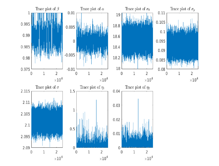
Figure S-1: Trace plots for the parameters for data simulated from 3-component GP mixtures.

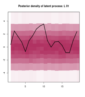
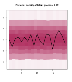
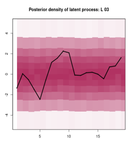
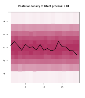
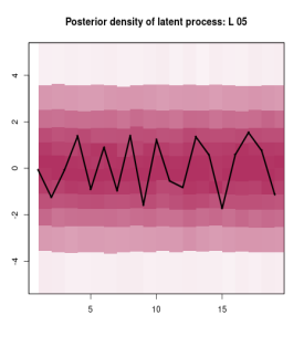
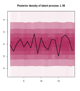
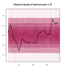
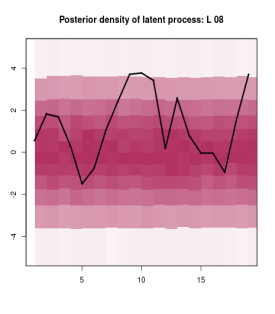
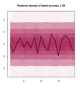
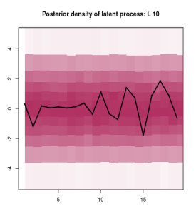
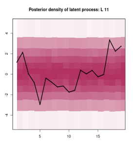
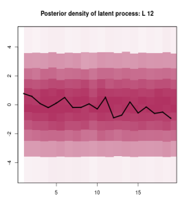
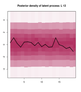
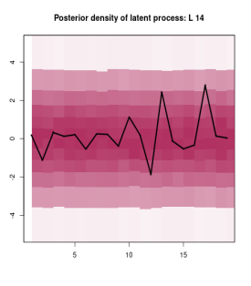
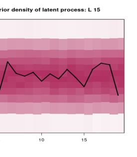
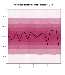
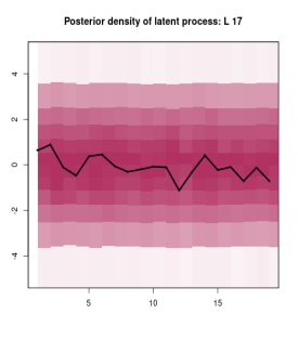
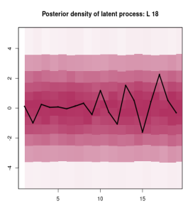
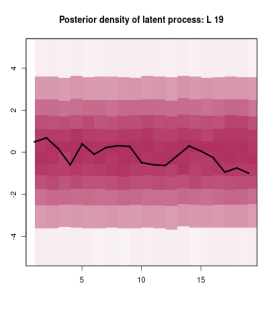
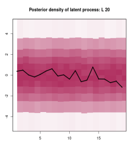
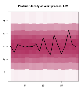
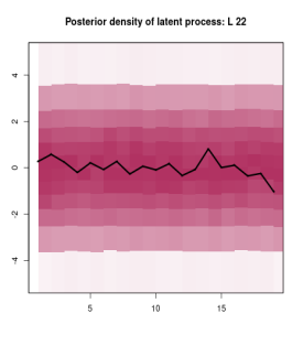
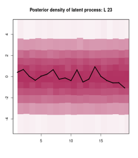
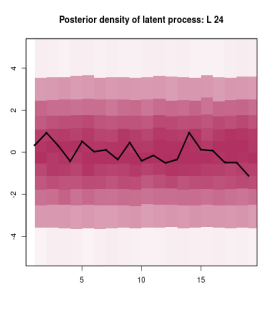
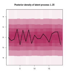
Figure S-2: Posterior densities of latent variables for the first 25 locations for data simulated from 3-component mixture of GPs. Higher the intensity of the colour, higher is the probability density. The black line represents the true values of the latent variables. $L_{i},i=1,\ldots,25$, denote the locations.

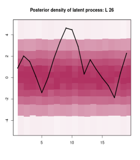
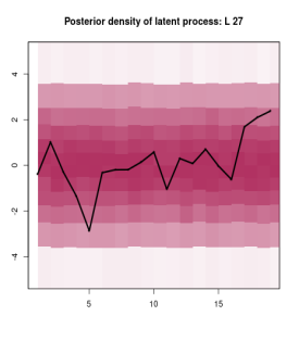
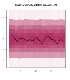
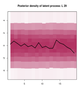
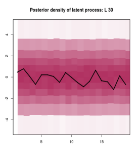
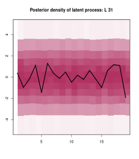
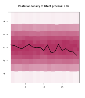
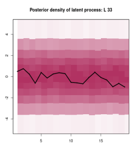
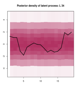
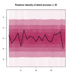
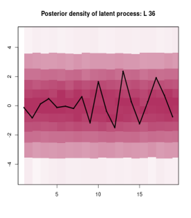
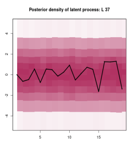
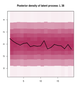
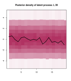
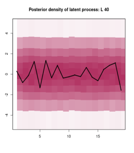
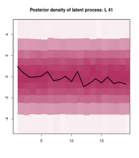
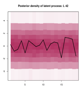
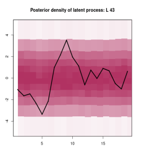
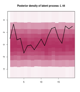
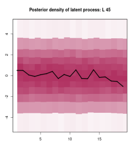
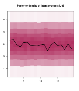
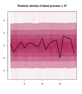
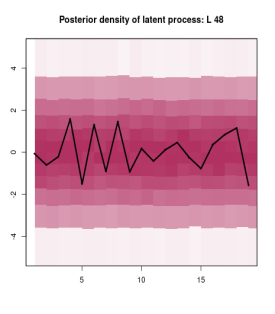
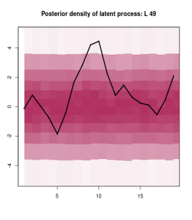
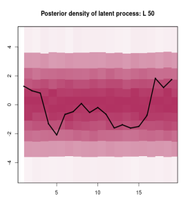
Figure S-3: Posterior densities of latent variables for the last 25 locations for data simulated from 3-component mixture of GPs. Higher the intensity of the colour, higher is the probability density. The black line represents the true values of the latent variables. $L_{i},i=26,\ldots,50$, denote the locations.

S-6 Trace plots of the parameters and the posterior densities of the complete time series of the latent variables for the mixture of GQNs

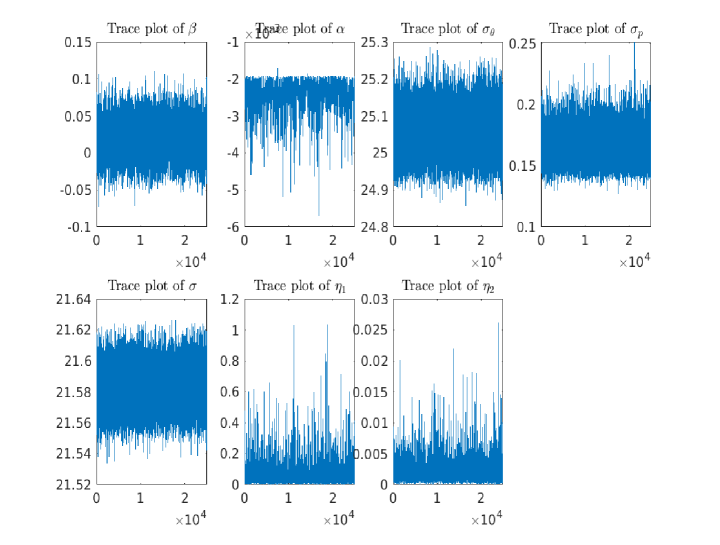
Figure S-4: Trace plots for the parameters for data simulated from mixture of GQNs.

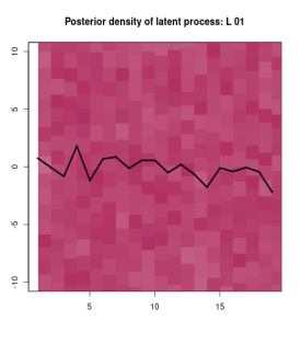
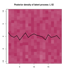
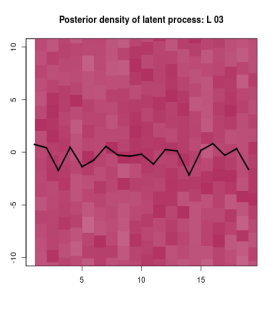
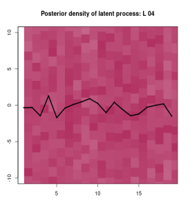
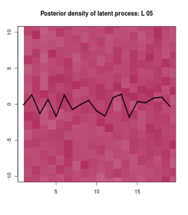
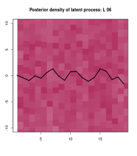
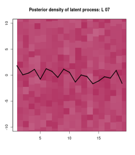
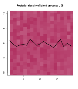
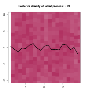
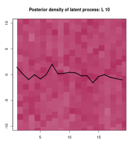
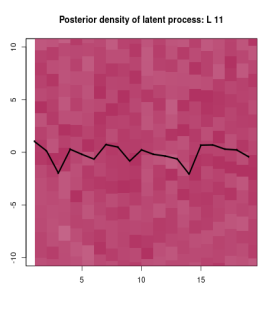
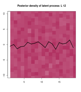
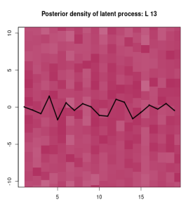
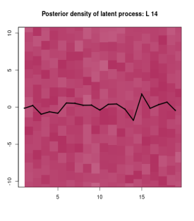
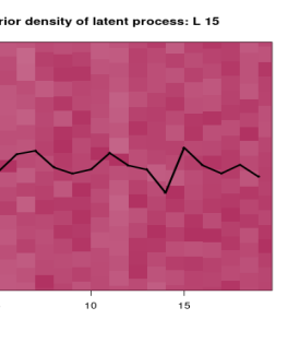
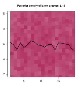
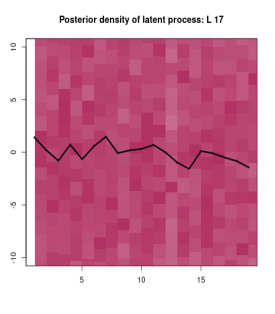
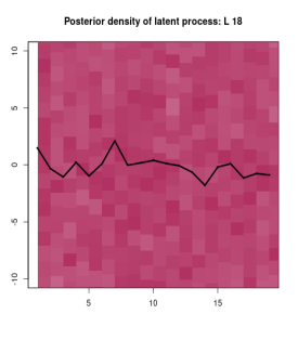
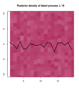
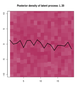
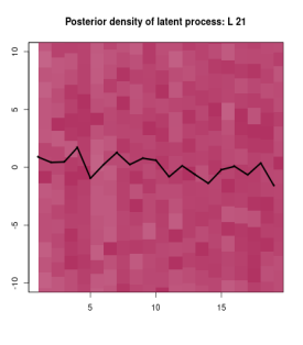
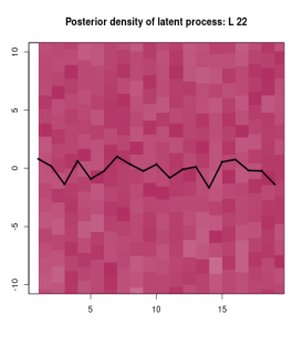
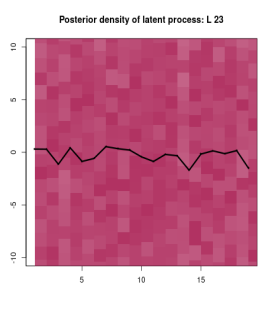
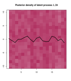
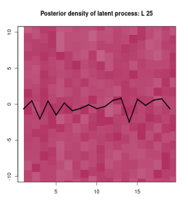
Figure S-5: Posterior densities of latent variables for the first 25 locations for data simulated from mixture of two GQNs. Higher the intensity of the colour, higher is the probability density. The black line represents the true values of the latent variables. $L_{i},i=1,\ldots,25$, denote the locations.

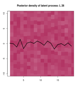
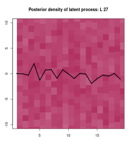
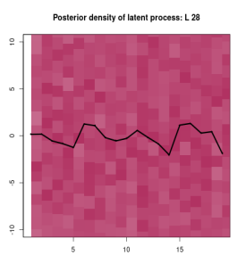
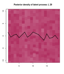
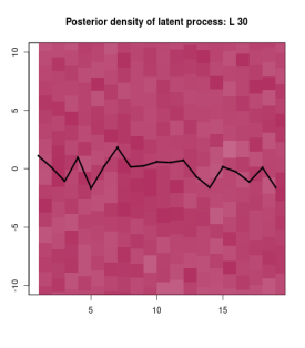
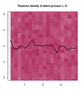
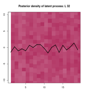
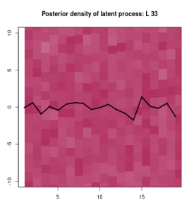
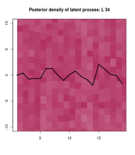
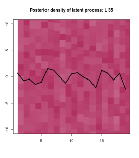
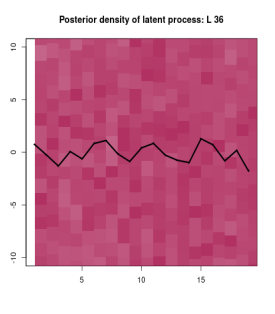
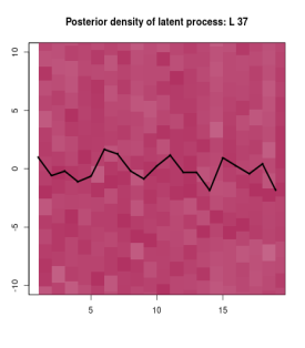
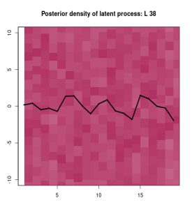
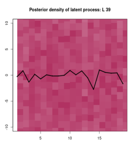
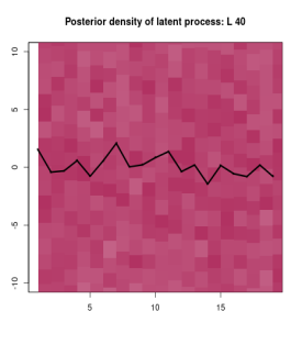
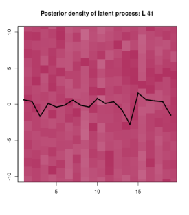
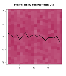
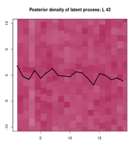
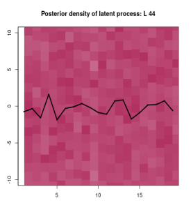
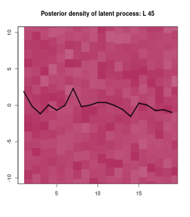
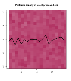
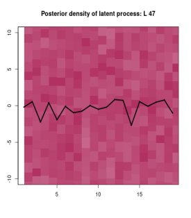
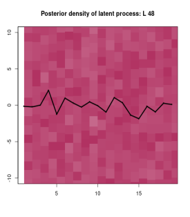
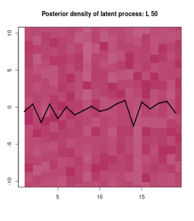
Figure S-6: Posterior densities of latent variables for the last 25 locations for data simulated from mixture of two GQNs. Higher the intensity of the colour, higher is the probability density. The black line represents the true values of the latent variables. $L_{i},i=26,\ldots,50$, denote the locations.

S-7 Trace plots of the parameters and the posterior densities of the complete time series of the latent variables for the Alaska temperature data

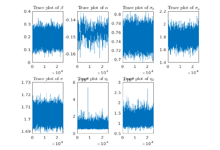
Figure S-7: Trace plot for the parameters except for $\eta_{3}$ corresponding to the Alaska temperature data.

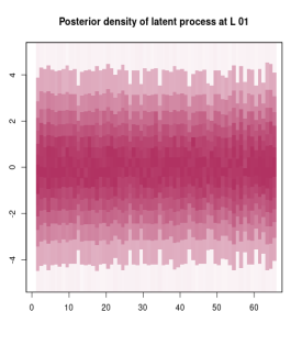
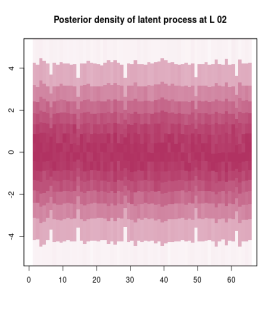
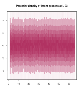
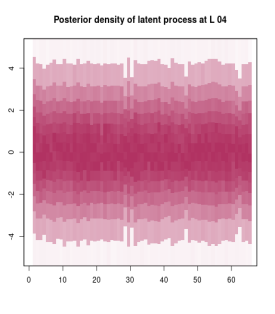
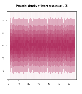
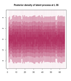
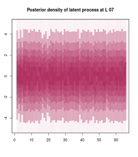
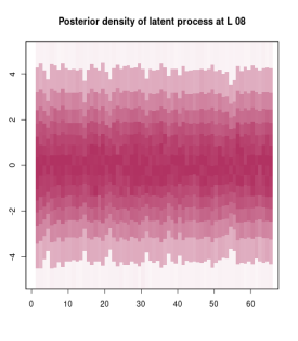
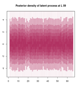
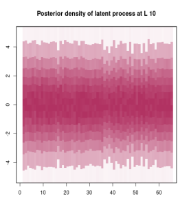
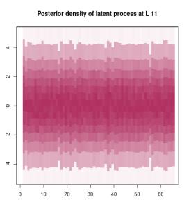
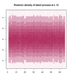
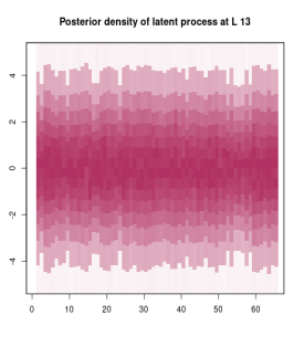
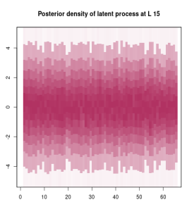
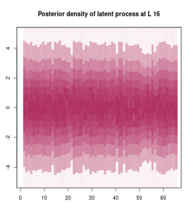
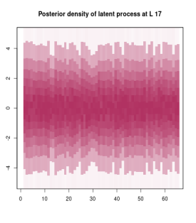
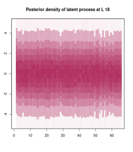
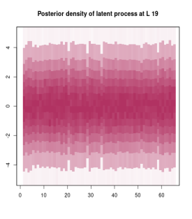
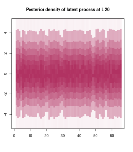
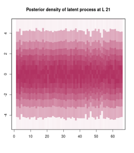
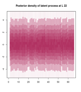
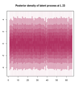
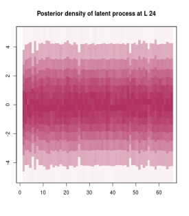
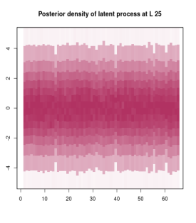
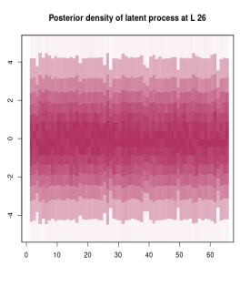
Figure S-8: Posterior densities of the latent variables at 26 locations in Alaska and its surroundings corresponding to the annual detrended temperature data. Higher the intensity of the colour, higher is the probability density.

S-8 Trace plots of the parameters and the posterior densities of the complete time series of the latent variables for the sea surface temperature data

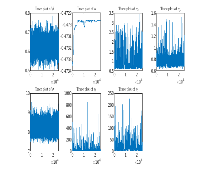
Figure S-9: Trace plots of the parameters except for $\eta_{3}$ for the sea surface temperature data.

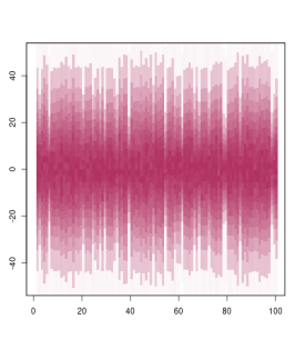
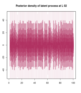
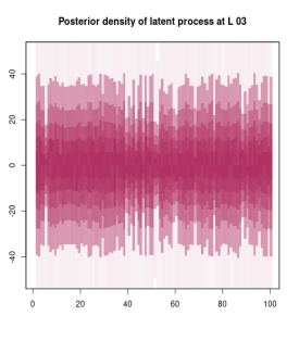
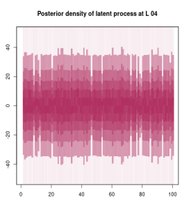
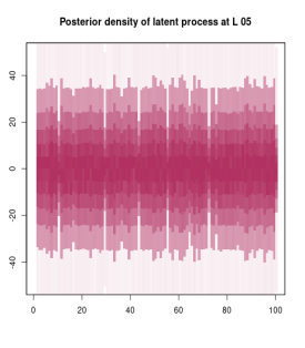
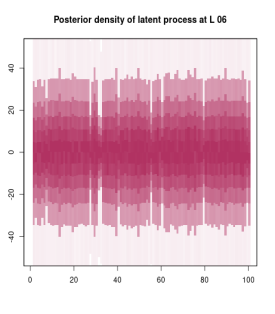
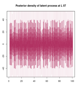
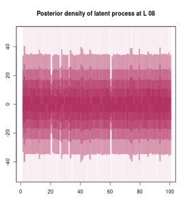
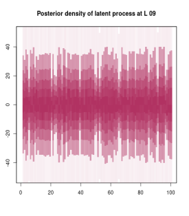
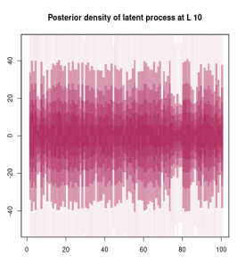
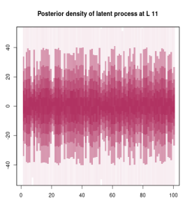
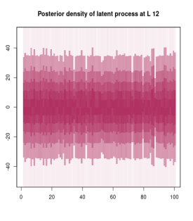
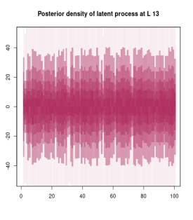
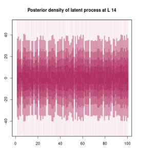
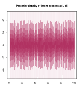
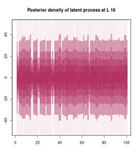
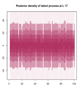
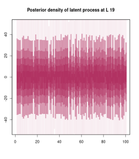
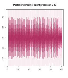
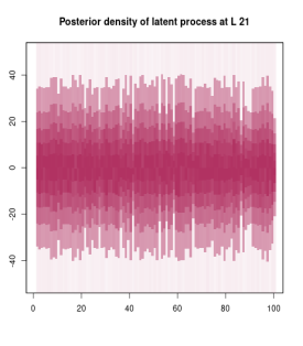
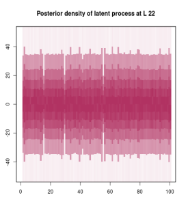
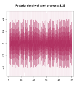
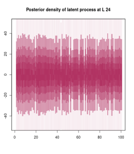
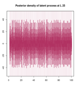
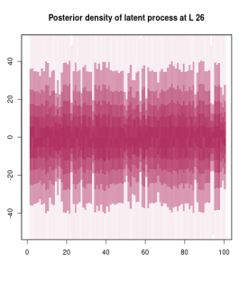
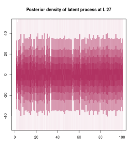
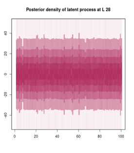
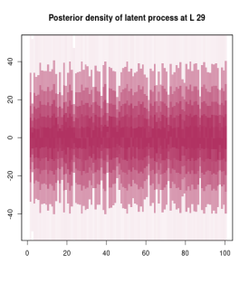
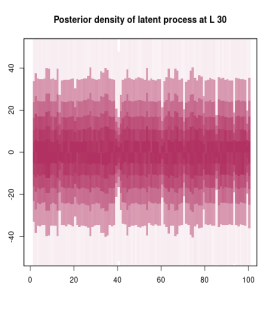
Figure S-10: Posterior densities of the latent variables at 30 locations of the sea surface temperature data. Higher the intensity of the colour, higher is the probability density.

S-9 Stationarity, convergence of lagged correlations to zero and non-Gaussianity of the detrended Alaska data process

S-9.1 Stationarity of the detrended Alaska data process

To check if the data arrived from a stationary or nonstationary process, we resorted to the recursive Bayesian theory and methods developed by [23]. In a nutshell, their key idea is to consider the Kolmogorov-Smirnov distance between distributions of data associated with local and global space-times. Associated with the $j$-th local space-time region is an unknown probability $p_{j}$ of the event that the underlying process is stationarity when the observed data corresponds to the $j$-th local region and the Kolmogorov-Smirnov distance falls below $c_{j}$, where $c_{j}$ is any non-negative sequence tending to zero as $j$ tends to infinity. With suitable priors for $p_{j}$, [23] constructed recursive posterior distributions for $p_{j}$ and proved that the underlying process is stationary if and only if for sufficiently large number of observations in the $j$-th region, the posterior of $p_{j}$ converges to one as $j\rightarrow\infty$. Nonstationarity is the case if and only if the posterior of $p_{j}$ converges to zero as $j\rightarrow\infty$.

In our implementation of the ideas of [23], we set the $j$-th local region to be the entire time series for the spatial location $\mbox{\boldmath{$s$}}_{j}$, for $j=1,\ldots,29$. Thus, the size of each local region is $65$. We choose $c_{j}$ to be of the same nonparametric, dynamic and adaptive form as detailed in [23]. The dynamic form requires an initial value for the sequence. In practice, the choice of the initial value usually has significant effect on the convergence of the posteriors of $p_{j}$, and so, the choice must be carefully made. However, in our case, for all initial values that we experimented with, lying between 0.05 and 1, the recursive Bayesian procedure led to the conclusion of stationarity of the underlying spatio-temporal process.

We implemented the idea with our parallelised C code on $29$ parallel processors of a VMWare of Indian Statistical Institute; the time taken is less than a second. For the initial value $0.05$, Figure S-11 displays the means of the posteriors of $p_{j}$; $j=1,\ldots,29$, showing convergence to 1. The respective posterior variances are negligibly small and hence not shown. Thus, the detrended spatio-temporal process that generated the Alaska data, can be safely regarded as stationary.

Figure S-11: Alaska data analysis: detection of strict stationarity.

S-9.2 Convergence of lagged spatio-temporal correlations to zero for the Alaska data

Recall that one major purpose of our Hamiltonian spatio-temporal model is to emulate the property of most real datasets that the lagged spatio-temporal correlations tend to zero as the spatio-temporal lag tends to infinity, irrespective of stationarity or nonstationarity. Here we compute the lagged correlations on $30$ parallel processors on our VMWare, each processor computing the correlation for a partitioned interval of lag $\|\mbox{\boldmath{$h$}}\|$ such that the interval is associated with sufficient data making the correlation well-defined. The time taken for this exercise are a few seconds. Figure S-12 demonstrates convergence of the lagged spatio-temporal correlations to zero; with larger amount of data such demonstration would have been more convincing.

Figure S-12: Alaska data analysis: lagged spatio-temporal correlations converging to zero.

S-9.3 Non-Gaussianity of the Alaska data

Simple quantile-quantile plots (not shown for brevity) revealed that the distributions of the time series data at the spatial locations, distributions of the spatial data at the time points, and the overall distribution of the entire dataset, are far from normal. Thus, traditional Gaussian process based models of the underlying spatio-temporal process are ruled out. Since the temporal distributions at the spatial locations and the spatial distributions at different time points are also much different, it does not appear feasible to consider parametric stochastic process models for the data. These seem to make the importance of our nonparametric Hamiltonian process more pronounced.

References

- Furrer and Sain [2009] Reinhard Furrer and Stephan R Sain. Spatial model fitting for large datasets with applications to climate and microarray problems. Statistics and Computing, 19(2):113–128, 2009.
- Jun et al. [2008] Mikyoung Jun, Reto Knutti, and Douglas W Nychka. Spatial analysis to quantify numerical model bias and dependence: how many climate models are there? Journal of the American Statistical Association, 103(483):934–947, 2008.
- Sain et al. [2011] Stephan R Sain, Reinhard Furrer, and Noel Cressie. A spatial analysis of multivariate output from regional climate models. The Annals of Applied Statistics, pages 150–175, 2011.
- Sang et al. [2011] Huiyan Sang, Mikyoung Jun, and Jianhua Z Huang. Covariance approximation for large multivariate spatial data sets with an application to multiple climate model errors. The Annals of Applied Statistics, pages 2519–2548, 2011.
- Smith et al. [2009] Richard L Smith, Claudia Tebaldi, Doug Nychka, and Linda O Mearns. Bayesian modeling of uncertainty in ensembles of climate models. Journal of the American Statistical Association, 104(485):97–116, 2009.
- Tebaldi and Sansó [2009] Claudia Tebaldi and Bruno Sansó. Joint projections of temperature and precipitation change from multiple climate models: a hierarchical bayesian approach. Journal of the Royal Statistical Society: Series A (Statistics in Society), 172(1):83–106, 2009.
- Cox and Isham [1988] David Roxbee Cox and Valerie Isham. A simple spatial-temporal model of rainfall. Proceedings of the Royal Society of London. A. Mathematical and Physical Sciences, 415(1849):317–328, 1988.
- Sanso and Guenni [1999] Bruno Sanso and Lelys Guenni. Venezuelan rainfall data analysed by using a bayesian space–time model. Journal of the Royal Statistical Society: Series C (Applied Statistics), 48(3):345–362, 1999.
- Sahu et al. [2010] Sujit K Sahu, Alan E Gelfand, and David M Holland. Fusing point and areal level space–time data with application to wet deposition. Journal of the Royal Statistical Society: Series C (Applied Statistics), 59(1):77–103, 2010.
- Bruno et al. [2009] Francesca Bruno, Peter Guttorp, Paul D Sampson, and Daniela Cocchi. A simple non-separable, non-stationary spatiotemporal model for ozone. Environmental and ecological statistics, 16(4):515–529, 2009.
- Dou et al. [2010] Yiping Dou, Nhu D Le, and James V Zidek. Modeling hourly ozone concentration fields. The Annals of applied statistics, 4(3):1183–1213, 2010.
- Guttorp et al. [1994] Peter Guttorp, Wendy Meiring, and Paul D Sampson. A space-time analysis of ground-level ozone data. Environmetrics, 5(3):241–254, 1994.
- Huerta et al. [2004] Gabriel Huerta, Bruno Sansó, and Jonathan R Stroud. A spatiotemporal model for mexico city ozone levels. Journal of the Royal Statistical Society: Series C (Applied Statistics), 53(2):231–248, 2004.
- Giannitrapani et al. [2006] Marco Giannitrapani, Adrian Bowman, Marian Scott, and Ron Smith. Sulphur dioxide in europe: Statistical relationships between emissions and measured concentrations. Atmospheric Environment, 40(14):2524–2532, 2006.
- Holland et al. [2000] David M Holland, Oliveira Victor De, Lawrence H Cox, and Richard L Smith. Estimation of regional trends in sulfur dioxide over the eastern united states. Environmetrics: The official journal of the International Environmetrics Society, 11(4):373–393, 2000.
- Paciorek et al. [2009] Christopher J Paciorek, Jeff D Yanosky, Robin C Puett, Francine Laden, and Helen H Suh. Practical large-scale spatio-temporal modeling of particulate matter concentrations. The Annals of Applied Statistics, pages 370–397, 2009.
- Amini et al. [2016] Heresh Amini, Seyed-Mahmood Taghavi-Shahri, Sarah B Henderson, Vahid Hosseini, Hossein Hassankhany, Maryam Naderi, Solmaz Ahadi, Christian Schindler, Nino Künzli, and Masud Yunesian. Annual and seasonal spatial models for nitrogen oxides in tehran, iran. Scientific reports, 6(1):1–11, 2016.
- Chakraborty et al. [2010] Avishek Chakraborty, Alan E Gelfand, Adam M Wilson, Andrew M Latimer, and John A Silander Jr. Modeling large scale species abundance with latent spatial processes. The Annals of Applied Statistics, 4(3):1403–1429, 2010.
- Deng et al. [2009] Jin S Deng, Ke Wang, Yang Hong, and Jia G Qi. Spatio-temporal dynamics and evolution of land use change and landscape pattern in response to rapid urbanization. Landscape and urban planning, 92(3-4):187–198, 2009.
- Banerjee et al. [2014] Sudipto Banerjee, Bradley P Carlin, and Alan E Gelfand. Hierarchical modeling and analysis for spatial data. CRC press, 2014.
- Sampson and Guttorp [1992] Paul D Sampson and Peter Guttorp. Nonparametric estimation of nonstationary spatial covariance structure. Journal of the American Statistical Association, 87(417):108–119, 1992.
- Das and Bhattacharya [2023] Moumita Das and Sourabh Bhattacharya. A kernel-enriched order-dependent nonparametric spatio-temporal process. Spatial Statistics, 55:100751, 2023.
- Roy and Bhattacharya [2020] Sucharita Roy and Sourabh Bhattacharya. Bayesian characterizations of properties of stochastic processes with applications. arXiv preprint arXiv:2005.00035, 2020.
- Bhattacharya [2021] Sourabh Bhattacharya. Bayesian lévy-dynamic spatio-temporal process: Towards big data analysis. arXiv preprint arXiv:2105.08451, 2021.
- Paciorek [2003] Christopher Joseph Paciorek. Nonstationary Gaussian processes for regression and spatial modelling. PhD thesis, Carnegie Mellon University, 2003.
- Gelfand et al. [2010] Alan E Gelfand, Peter Diggle, Peter Guttorp, and Montserrat Fuentes. Handbook of spatial statistics. CRC press, 2010.
- Damian et al. [2001] Doris Damian, Paul D Sampson, and Peter Guttorp. Bayesian estimation of semi-parametric non-stationary spatial covariance structures. Environmetrics: The official journal of the International Environmetrics Society, 12(2):161–178, 2001.
- Schmidt and O’Hagan [2003] Alexandra M Schmidt and Anthony O’Hagan. Bayesian inference for non-stationary spatial covariance structure via spatial deformations. Journal of the Royal Statistical Society: Series B (Statistical Methodology), 65(3):743–758, 2003.
- Higdon [1998] David Higdon. A process-convolution approach to modelling temperatures in the north atlantic ocean. Environmental and Ecological Statistics, 5(2):173–190, 1998.
- Higdon et al. [1999] D Higdon, J Swall, and J Kern. Non-stationary spatial modeling. In J Bernardo, J Berger, A Dawid, and A Smith, editors, Bayesian Statistics 6, pages 761–768. Oxford University Press, Oxford, U.K., 1999.
- Fuentes and Smith [2001] M. Fuentes and R.L. Smith. A new class of nonstationary spatial model. Technical report, North Carolina State University, 2001.
- Higdon [2002] Dave Higdon. Space and space-time modeling using process convolutions. In W. Anderson Clive, Barnett Vic, C. Chatwin Philip, and Abdel H. El-Shaarawi, editors, Quantitative methods for current environmental issues, pages 37–56. Springer, 2002.
- Fuentes [2002] Montserrat Fuentes. Spectral methods for nonstationary spatial processes. Biometrika, 89(1):197–210, 2002.
- Paciorek and Schervish [2006] Christopher J Paciorek and Mark J Schervish. Spatial modelling using a new class of nonstationary covariance functions. Environmetrics: The official journal of the International Environmetrics Society, 17(5):483–506, 2006.
- Lindgren et al. [2011] Finn Lindgren, Håvard Rue, and Johan Lindström. An explicit link between gaussian fields and gaussian markov random fields: the stochastic partial differential equation approach. Journal of the Royal Statistical Society Series B: Statistical Methodology, 73(4):423–498, 2011.
- Blangiardo and Cameletti [2015] Marta Blangiardo and Michela Cameletti. Spatial and spatio-temporal Bayesian models with R-INLA. John Wiley & Sons, 2015.
- Bolin and Lindgren [2011] David Bolin and Finn Lindgren. Spatial models generated by nested stochastic partial differential equations, with an application to global ozone mapping. The Annals of Applied Statistics, pages 523–550, 2011.
- Ingebrigtsen et al. [2014] Rikke Ingebrigtsen, Finn Lindgren, and Ingelin Steinsland. Spatial models with explanatory variables in the dependence structure. Spatial Statistics, 8:20–38, 2014.
- Lindgren et al. [2022] Finn Lindgren, David Bolin, and Håvard Rue. The spde approach for gaussian and non-gaussian fields: 10 years and still running. Spatial Statistics, 50:100599, 2022.
- Lindgren and Rue [2015] Finn Lindgren and Håvard Rue. Bayesian spatial modelling with r-inla. Journal of statistical software, 63(19), 2015.
- Gómez-Rubio [2020] Virgilio Gómez-Rubio. Bayesian inference with INLA. CRC Press, 2020.
- Gelfand et al. [2005] Alan E Gelfand, Athanasios Kottas, and Steven N MacEachern. Bayesian nonparametric spatial modeling with dirichlet process mixing. Journal of the American Statistical Association, 100(471):1021–1035, 2005.
- Fuentes and Reich [2013] Montserrat Fuentes and Brian Reich. Multivariate spatial nonparametric modelling via kernel processes mixing. Statistica Sinica, 23(1), 2013.
- Duan et al. [2009] Jason A Duan, Alan E Gelfand, and CF Sirmans. Modeling space-time data using stochastic differential equations. Bayesian analysis, 4(4):733–758, 2009.
- Cressie and Wikle [2015] Noel Cressie and Christopher K Wikle. Statistics for spatio-temporal data. John Wiley & Sons, 2015.
- Guha [2017] Suman Guha. Some Theoretical and Methodological Contributions to the Dynamic Modeling of Discrete-Time Spatial Time Series Data. PhD thesis, Indian Statistical Institute, Kolkata, 2017.
- Betancourt [2017] Michael Betancourt. A conceptual introduction to hamiltonian monte carlo. arXiv preprint arXiv:1701.02434, 2017.
- Cheung and Beck [2009] Sai Hung Cheung and James L Beck. Bayesian model updating using hybrid monte carlo simulation with application to structural dynamic models with many uncertain parameters. Journal of engineering mechanics, 135(4):243–255, 2009.
- Young [2014] Peter Young. The leapfrog method and other symplectic algorithms for integrating newton’s laws of motion. Lecture notes in University of california, santa cruz, 2014.
- Stein [1999a] M. L. Stein. Interpolation of Spatial Data: Some Theory for Kriging. Springer-Verlag, New York, Inc, 1999a.
- Rusmassen and Williams [2006] CE Rusmassen and CKI Williams. Gaussian process for machine learning. the MIT Press, 2006.
- Stein [1999b] Michael L. Stein. Interpolation of Spatial Data. Springer, New York, 1999b.
- Zhang [2004] Hao Zhang. Inconsistent estimation and asymptotically equal interpolations in model-based geostatistics. Journal of the American Statistical Association, 99(465):250–261, 2004.
- Banerjee [2020] Sudipto Banerjee. Modeling massive spatial datasets using a conjugate bayesian linear modeling framework. Spatial Statistics, 37:100417, 2020.
- Wikle and Hooten [2010] Christopher K Wikle and Mevin B Hooten. A general science-based framework for dynamical spatio-temporal models. Test, 19(3):417–451, 2010.
- Das and Bhattacharya [2019] Moumita Das and Sourabh Bhattacharya. Transdimensional transformation based markov chain monte carlo. Brazilian Journal of Probability and Statistics, 33:87–138, 2019.
- Banerjee et al. [2015] Sudipto Banerjee, Bradley P Carlin, and Alan E Gelfand. Hierarchical Modeling and Analysis for Spatial Data. CRC press, Boca Raton, Florida, 2nd edition, 2015.