Minority-Oriented Vicinity Expansion with Attentive Aggregation
for Video Long-Tailed Recognition

Abstract

A dramatic increase in real-world video volume with extremely diverse and emerging topics naturally forms a long-tailed video distribution in terms of their categories, and it spotlights the need for Video Long-Tailed Recognition (VLTR). In this work, we summarize the challenges in VLTR and explore how to overcome them. The challenges are: (1) it is impractical to re-train the whole model for high-quality features, (2) acquiring frame-wise labels requires extensive cost, and (3) long-tailed data triggers biased training. Yet, most existing works for VLTR unavoidably utilize image-level features extracted from pretrained models which are task-irrelevant, and learn by video-level labels. Therefore, to deal with such (1) task-irrelevant features and (2) video-level labels, we introduce two complementary learnable feature aggregators. Learnable layers in each aggregator are to produce task-relevant representations, and each aggregator is to assemble the snippet-wise knowledge into a video representative. Then, we propose Minority-Oriented Vicinity Expansion (MOVE) that explicitly leverages the class frequency into approximating the vicinity distributions to alleviate (3) biased training. By combining these solutions, our approach achieves state-of-the-art results on large-scale VideoLT and synthetically induced Imbalanced-MiniKinetics200. With VideoLT features from ResNet-50, it attains 18% and 58% relative improvements on head and tail classes over the previous state-of-the-art method, respectively.

1 Introduction

With the development of online video platforms, recent years have witnessed a rapid growth in interest in learning from video. However, unlike the image domain, video has an additional temporal dimension which requires huge memory and computation cost. Thus, it has been an inevitably common approach to utilize the extracted features using pretrained networks. (Brattoli et al. 2020; Xu et al. 2020; Lin et al. 2019). However, this raises the issue of using task-irrelevant features in downstream tasks due to the domain gap between datasets to pretrain the network and be utilized.VLTR is not an exception since its focus is to learn from a vast amount of videos being collected via online platforms.

Data imbalance, a natural phenomenon in these real-world datasets, is detrimental since it triggers biased training that results in the model performing poorly on tail classes (Li, Cheung, and Lu 2021; Zhang et al. 2021c). To overcome the difficulty, there were numerous approaches in the image domain such as reweighting and resampling (Cao et al. 2019; Fan et al. 2017; Menon et al. 2020; Ren et al. 2020; Shu et al. 2019). However, directly applying these techniques to the video domain is impractical because acquiring accurate frame-wise supervision for massive video datasets is usually cumbersome, and some snippets are no more than background frames (Zhang et al. 2021b). Thus, data imbalance in the video domain should be considered with the issue of learning from task-irrelevant features and weakly-labeled problems that only the video-level label is available.

To this end, we first employ learnable feature aggregators to rectify and aggregate the frame-wise representations at a video-level where the weak labels are available. Previously, Framestack (Zhang et al. 2021b) stuck with the frame-level balancing technique since not all snippets contain informative clues. Nevertheless, our intuition is that snippet-wise feature in weakly labeled settings is detrimental since the precise labels cannot be assigned. Label cleaning (Feng, Hong, and Zheng 2021; Zhong et al. 2019) that generates reliable snippet-wise pseudo labels, is also impractical since neural networks are poor at generalizing on the minority. Therefore, we argue that weakly labeled VLTR should be treated at the video-level where noisy background scenes are watered down. Subsequently, we propose Minority-Oriented Vicinity Expansion (MOVE) to prevent the majority-biased training and overfitting to the partial data of the tail classes. Specifically, we expand the empirical distribution of sparse minorities by dynamic extrapolation and extend the distribution by assigning more linearly designed space between the class distributions to the minority than the majority with calibrated interpolation. Overall, our framework comprises two phases as shown in Fig. 1.

Figure 1: Overall flow. Given input feature $\mathbf{x}$, our proposed Dynamic Frame Sampler (DFS) is firstly performed as an effective augmentation tool when developing a video prototype (Sec.3.1). These features are condensed into task-relevant video representation by two aggregators (Sec.2). After concatenation, a balanced training of the classifier based on expanding and extending the representation space of the minorities is led by our proposed MOVE (Sec.3.1). At inference, only the learnable feature aggregators and the classifier are used for prediction.

Our key contributions are:

• We summarize the challenges in VLTR and empirically verify the importance of handling these challenges with our ablation studies. We believe that our findings clearly segment and introduce the research direction.

• We introduce learnable feature aggregators as an effective tool to obtain task-relevant and label-consistent features in weakly-labeled VLTR. Experiments demonstrate that baselines are significantly improved with our aggregators.

• We propose Minority-Oriented Vicinity Expansion to generalize the model to long-tailed data distribution by alleviating the biased training.

• Our overall approach is verified to be superior to existing state-of-the-art methods with extensive experiments.

• We newly introduce an imbalanced video classification benchmark, Imbalanced-MiniKinetics200, sampled from Kinetics-400 to evaluate diverse imbalanced scenarios.

2 Learnable Feature Aggregator

2.1 Background and problems

Oftentimes, it is unrealistic to re-train the entire network to get access to the quality of feature maps. It is especially true in the video domain because of the huge size of the videos. Thus, it has been common to use popular pretrained backbones. Likewise, VLTR also aims to learn from real-world data collected day and night. Yet, video recognition obviously depends on the quality of class-discriminative features while pretrained networks may not fit for extracting such quality due to the domain gap between datasets (Choi et al. 2020).

In addition, processing snippet-wise features require accurate snippet-wise label information that is accompanied by extensive human labor. To extract reliable supervision in a weakly labeled setting, label cleaning has been proposed where the model iteratively assigns and corrects the snippet-wise labels with its predictions (Feng, Hong, and Zheng 2021; Zhong et al. 2019). However, under the circumstance where the model’s predictions are not precise, especially on tail classes, it is difficult to proofread the label precisely. Therefore, we argue that it is better to modify snippet-wise features to match the degree of trustworthy supervision at the video-level rather than the other way around, e.g., label cleaning. In short, feature aggregation addresses the level mismatch between given snippet-wise feature representation and video-wise supervision, alleviating the label uncertainty.

Figure 2: Capability of localizing class-discriminative frames of two aggregators introduced in Sec. 2. ’trumpet performance’ and ’jugglingBall’ classes in VideoLT are used, and the X-axis of (a) and (b) are shared. (a) Per-frame attention score ($\textit{QK}^{\mathsf{T}}/\sqrt{d}$) in self-attentive aggregator. As high attention scores are given to frames deeply involving class information (blue arrow) and low scores on noisy frames (yellow arrow), it is obvious that the video prototype feature is well supplemented with class-relative local clues. In Sec. 4.3, we further analyze how our self-attentive aggregator achieves more gains than the naive use of MSA by addressing two subproblems in VLTR. (b) Per-frame degree of adjacency to each cluster in codebook-attentive aggregator. It can be noticed that degree of adjacency to all clusters reflects the frame similarity. Similar frames are assigned with similar adjacency values (blue dotted lines), whereas others are not (yellow dotted lines). These scores clearly describe how well our aggregators understand and represent the video.

2.2 Generating task-relevant and label-consistent representation

With features from pretrained networks, we aim to produce task-relevant discriminative representations and address a weakly labeled problem when it concurrently exists with data imbalance. To manage these, we introduce two learnable feature aggregators: self-attentive and codebook-attentive aggregators. Specifically, the role of learnable layers within these aggregators is to develop task-relevant representations overcoming the domain gap between the dataset to pretrain the network and the target dataset for the downstream task. Label uncertainty from weak labels is also relieved by the aggregation process to equalize the level of data point and its supervision. Note that the loss of information while feature compression, is not critical since two complementary aggregators alleviate the issue and a well-chosen prototype is often enough to achieve strong performance (Buch et al. 2022).

Self-attentive aggregator. Self-attention (SA) (Vaswani et al. 2017; Dosovitskiy et al. 2022) aggregates feature maps with normalized importance that indicates the relationship between a token and all other tokens. Specifically, given $i$-th input feature $\mathbf{x}^{i}$ from a pretrained network to linearly project each query Q, key K, and value V, SA operates as follows:

$$\mathbf{\hat{x}}^{i}=\text{Softmax}\big{(}\textit{QK}^{\mathsf{T}}/{\sqrt{d}}\big{)}\textit{V},$$ (1)

where $d$ is the feature dimension of feature $\mathbf{x}^{i}$. Multihead Self-Attention (MSA) is an extension of SA where multiple heads exist to implement self-attention operations. Such MSA can be interpreted as an ensemble over SA for searching robust attention maps by considering different representations.

With the property of local attention, our focus is to efficiently generate video-level representation. Therefore, we simply modify MSA to introduce Prototypical Self-Attention (PSA) that complements the global feature with the snippet-level local clues. In PSA, we project Pool$(\mathbf{x}^{i})$ into Q instead of projecting $\mathbf{x}^{i}$ where Pool$()$ denotes the function for average pooling to aggregate temporal information. Then, global feature, Pool$(\mathbf{x}^{i})$, is supplemented with the informative local clues from frame-wise features $\mathbf{x}^{i}$ to represent the video instance. As shown in Fig. 2, meaningful local clues are highly likely to be assembled to the prototype, while frames with class-meaningless features are not. Consequently, PSA yields $\mathbf{\hat{x}}^{i}$, the class-discriminative prototype at the same level as weak labels. Additionally, it has its benefits in efficiency since only the prototype is re-expressed with other snippets.

Codebook-attentive aggregator. NetVLAD (Arandjelovic et al. 2016), the differentiable form of VLAD (Jégou et al. 2010), is another strategy to aggregate a set of features effectively. Generally, with the feature representation $\mathbf{x}^{i}\in\mathbb{R}^{T\times C}$ from a video stream as an input, VLAD assumes $K$ clusters $\boldsymbol{\mu}\in\mathbb{R}^{K\times C}$ in the global codebook. With the residues from these two vectors, VLAD outputs $C\times K$-dimensional representation $\tilde{\mathbf{x}}^{i}$:

$$\mathbf{\tilde{x}}^{i}_{c,k}=\sum^{T}_{t=1}\rho_{k}(\mathbf{x}^{i}_{t})(\mathbf{x}^{i}_{t,c}-\boldsymbol{\mu}_{k,c}),$$ (2)

where $\rho_{k}(\mathbf{x}_{t}^{i})$ is an indicator function that checks if the $k$-th cluster, $\boldsymbol{\mu}_{k}$, is the closest cluster from $\mathbf{x}_{t}^{i}$, the $t$-th component in the temporal dimension. $\mathbf{x}_{t,c}^{i}$ and $\boldsymbol{\mu}_{k,c}$ denote $c$-th dimension of $\mathbf{x}_{t}^{i}$ and $\boldsymbol{\mu}_{k}$, respectively. To make it differentiable, NetVLAD proposed to use softmax function for $\rho_{k}(\mathbf{x}_{t}^{i})$ as:

$$\rho_{k}(\mathbf{x}^{i}_{t})=\frac{e^{w_{k}^{\mathsf{T}}\mathbf{x}_{t}^{i}+b_{k}}}{\sum^{K}_{{k}^{\prime}=1}e^{w_{{k}^{\prime}}^{\mathsf{T}}\mathbf{x}^{i}_{t}+b_{k^{\prime}}}},$$ (3)

where $w_{k}$, $b_{k}$, and $\boldsymbol{\mu}_{k}$ are trainable parameters for $k$-th cluster in NetVLAD, respectively. Since the operation has the property of sharing the global codebook to express every video, we employ it as a codebook-attentive aggregator to represent the global relationship. Note that, although NetVLAD itself is not a part of our contribution, we believe that utilizing it together with the self-attentive aggregator to minimize information loss by complementing each other and the following discussion has a worthwhile technical contribution. In Fig. 2, the video understanding capability of the codebook-attentive aggregator is demonstrated as similar scenes exhibit a similar degree of adjacency to each cluster.

Discussion. Whereas the self-attentive aggregator considers internal relationships within videos to make class-relative representation, the codebook-attentive aggregator utilizes global relationships with clusters to implement the fine-grained discrimination beyond the class level. In Fig. 2, it is shown that attention scores in (a) are computed solely within a video instance (i.e., the relevance of each frame with respect to a video) to highlight task-relevant frames. On the other hand, the scores in (b) are defined with a codebook shared by all the instances to produce more fine-grained classification-friendly representations. In other words, it is rather straightforward that each module pursues a different way of deriving task-relevant and label-consistent representation, thereby supplementing each other (e.g., the codebook-attentive aggregator can complement the self-attentive aggregator when dominant backgrounds form noisy prototype in PSA). Thus, we define the final aggregated feature as:

$$\mathbf{z}^{i}=f_{\theta}(\mathbf{\hat{x}}^{i})\oplus f_{\phi}(\mathbf{\tilde{x}}^{i}),$$ (4)

where $f_{\theta}(\cdot)$ and $f_{\phi}(\cdot)$ are fully connected layers parameterized by $\theta$ and $\phi$, respectively, to project into a reduced dimension. $\oplus$ stands for concatenation. By combining these features, we achieve task-relevant and label-consistent video representation without much loss of information.

3 Minority-Oriented Vicinity Learning

As described in Sec.2, we propose and adopt aggregators to produce task-relevant representations and reduce the label uncertainty by uniting frame-level features into the prototype. Meanwhile, these do not provide a solution for balancing the biased training phrase with the long-tailed data distribution. Since it is widely known that the long-tailed distribution triggers the learning of head-biased decision boundaries (Li, Cheung, and Lu 2021; Park et al. 2021; Kang et al. 2020; Zhong et al. 2021a), we focus on readjusting such distorted boundaries. Still, there are insufficient samples for specific tail classes to achieve the adjustment. Therefore, we instead minimize the estimated vicinal risk from the calibrated vicinity to approximate the real data distribution.

Vicinal risk minimization. Given $Z$ and $Y$, a set of $i$-th input vector $\mathbf{z}^{i}$ and corresponding one-hot label $\mathbf{y}^{i}$, the objective of supervised learning is to find a hypothesis $h$ that $h:Z\to Y$. However, due to the unavailability of true distribution, the expected risk for learning $h$ cannot be computed. Although it is a natural practice to use empirical risk minimization instead, it is highly dependable on the quality of given data distribution. Then, (Chapelle et al. 2000) proposed Vicinal Risk Minimization (VRM) that approximates the expected risk with below equation:

$$R_{vic}(h) =\frac{1}{N}\sum_{i=1}^{N}\int\ell(h(\mathbf{z}),\mathbf{y}^{i})dP_{\mathbf{z}^{i},\mathbf{y}^{i}}(\mathbf{z},\mathbf{y})$$ (5)

$$=\frac{1}{N}\sum_{i=1}^{N}\ell(h(\tilde{\mathbf{z}}^{i}),\tilde{\mathbf{y}}^{i}),$$ (6)

where $P_{\mathbf{z}^{i},\mathbf{y}^{i}}(\mathbf{z},\mathbf{y})$ indicates a distribution in the vicinity of the data point ($\mathbf{z}^{i},\mathbf{y}^{i}$), and ($\tilde{\mathbf{z}}^{i},\tilde{\mathbf{y}}^{i}$) is a data point sampled from $P_{\mathbf{z}^{i},\mathbf{y}^{i}}(\mathbf{z},\mathbf{y})$. $N$ is the total number of training data. Simply put, the goal of VRM is to address the problem of missing data by discovering new kinds of patterns with the quality of density estimates. Therefore, we tailor VRM to the long-tailed problem by modeling the vicinity within/between samples and manipulating with the consideration of long-tailed sample gaps. We show how the vicinal distribution $P_{\mathbf{z}^{i},\mathbf{y}^{i}}(\mathbf{z},\mathbf{y})$ is defined by MOVE in the following subsection.

Figure 3: The key concept of MOVE. (Left) In imbalanced scenarios, boundaries are shifted and distorted towards the minority. (Center, Right) We propose two components of MOVE, namely dynamic extrapolation, and calibrated interpolation, that aim to smooth and balance the boundary by expanding and extending the tail vicinity distribution. DFS guides the extrapolation and interpolation to be focused on the minority.

3.1 Minority-Oriented Vicinity Expansion

Under the axiomatic circumstance where scarce minorities are relatively poor in their representations, we look for minority-enriched data distribution for the successful use of VRM. Specifically, biased training mostly consisting of the majority not only leads to shifted boundaries towards the minority but also forms complex boundaries since majority groups become dominant in-between the minority groups (Park et al. 2021) as illustrated in Fig. 3 (Left). To resolve these, we sequentially utilize two vicinal distributions formed by extrapolation and interpolation. Extrapolation is to deal with distorted boundaries by enriching the minority whereas interpolation is to calibrate the biased boundaries.

Prior to explaining how we design these distributions, we introduce how they differ the behaviors between classes. To be precise, we normalize the number of samples to be the tail-weighted criterion $\boldsymbol{\tau}$ for granting more weights on tail classes. Given $\mathbf{q}$, the vector consisting of number of samples for all classes, the $s$-th component of vector $\boldsymbol{\tau}$ is defined as:

$$\boldsymbol{\tau}_{s}=(\mathbf{q}_{s}-\mathbf{q}_{\text{min}})/(\mathbf{q_{\text{max}}}-\mathbf{q}_{\text{min}}).$$ (7)

$\mathbf{q}_{s}$, $\mathbf{q}_{\text{min}}$ and $\mathbf{q}_{\text{max}}$ stand for the $s$-th element, the minimum and maximum value in the vector $\mathbf{q}$, respectively.

Dynamic extrapolation. Extrapolation estimates new data beyond the empirical distribution. Although it is subject to generating samples with high uncertainty, we aim to generate probable data for tail classes to densify its vicinal distribution. This is particularly crucial for the minority since only the specific partial data points are available as shown in Fig. 3 (Left).

2.5					ResNet-50						ResNet-101
LT-Methods	Agg	All	H	M	T	A@1	A@5	All	H	M	T	A@1	A@5
2.5 Baseline	✗	0.499	0.675	0.553	0.376	0.650	0.828	0.516	0.687	0.568	0.396	0.663	0.837
LDAM (Cao et al. 2019)	✗	0.502	0.680	0.557	0.378	0.656	0.811	0.518	0.687	0.572	0.397	0.664	0.820
EQL (Tan et al. 2020)	✗	0.502	0.679	0.557	0.378	0.653	0.829	0.518	0.690	0.571	0.398	0.664	0.838
CBS (Kang et al. 2020)	✗	0.491	0.649	0.545	0.371	0.640	0.820	0.507	0.660	0.559	0.390	0.652	0.828
CB Loss (Cui et al. 2019)	✗	0.495	0.653	0.546	0.381	0.643	0.823	0.511	0.665	0.561	0.398	0.656	0.832
Mixup (Zhang et al. 2018)	✗	0.484	0.649	0.535	0.368	0.633	0.818	0.495	0.660	0.546	0.381	0.641	0.843
Framestack (Zhang et al. 2021b)	✗	0.516	0.683	0.569	0.397	0.658	0.834	0.532	0.695	0.584	0.417	0.667	0.843
Baseline	o	0.676	0.793	0.717	0.585	0.702	0.861	0.690	0.806	0.730	0.601	0.715	0.869
LDAM (Cao et al. 2019)	o	0.658	0.778	0.701	0.565	0.697	0.847	0.672	0.786	0.713	0.581	0.709	0.856
EQL (Tan et al. 2020)	o	0.676	0.794	0.717	0.585	0.704	0.862	0.690	0.805	0.729	0.602	0.714	0.870
CBS (Kang et al. 2020)	o	0.672	0.781	0.713	0.582	0.697	0.856	0.685	0.794	0.723	0.601	0.709	0.864
CB Loss (Cui et al. 2019)	o	0.681	0.784	0.717	0.601	0.695	0.847	0.693	0.793	0.728	0.616	0.705	0.854
Mixup (Zhang et al. 2018)	o	0.686	0.795	0.726	0.598	0.703	0.861	0.699	0.807	0.737	0.614	0.715	0.867
Framestack (Zhang et al. 2021b)	o	0.680	0.792	0.720	0.593	0.708	0.865	0.693	0.802	0.730	0.611	0.718	0.872
Ours	o	0.705	0.804	0.742	0.626	0.719	0.875	0.719	0.815	0.753	0.644	0.730	0.883
2.5

Table 1: Performance comparisons on VideoLT between long-tailed methods with features from ImageNet-pretrained ResNet-50 and ResNet-101. A@1, 5 are Top-1 and Top-5 accuracy and Agg indicates whether our learnable aggregators are applied or not.

Since our objective is to diversify with respect to sample numbers for each class, the sampling process for the extrapolation takes the number of samples into account. We implement this by allowing extrapolation between different representations of the same instance where such difference comes from the Dynamic Frame Sampler (DFS). With the frame index set $\mathbf{T}=\{1,...,T\}$ where $\left|\mathbf{T}\right|=T$, DFS generates a $t$-th frame of $s$-th class binary mask vector $\mathbf{m}$ as:

$$\mathbf{m}_{s,t}=\mathds{1}_{[t\in\mathbf{I}_{s}]},\\$$ (8)

where $\mathds{1}$ is an indicator function that assigns 1 if $t\in\mathbf{I}_{s}$ and 0 otherwise. $\mathbf{I}_{s}$ is a disposable index set for $s$-th class that it is randomly generated at every computation defined as:

$$\mathbf{I}_{s}\subseteq\mathbf{T},\;\left|\mathbf{I}_{s}\right|\sim\textrm{U}(\text{max}(\left\lfloor\boldsymbol{\tau}_{s}\times T\right\rfloor,\sigma),T),\;$$ (9)

where U denotes an uniform distribution and $\sigma$ is the minimum value for $\left|\mathbf{I}_{s}\right|$ to prevent generating video prototypes only with the backgrounds. Note that $\mathbf{m}_{s}$ is also resampled for every computation as $\mathbf{I}_{s}$ is disposable. As the $s$-th class has more samples, $\left|\mathbf{I}_{s}\right|$ would be bigger in which more similar candidates are used for the extrapolation, thereby not many variations in generating $\mathbf{m}_{s}$. For head classes, this maintains the given data distribution as its vicinity since the output of extrapolation would be similar to the given data points. On the other hand, different candidates are used for extrapolation for the minority to expand its vicinity as varying $\mathbf{I}_{s}$ and $\mathbf{m}_{s}$ can be sampled. Specifically, $\mathbf{m}_{s}$ is applied during the feature aggregation process. For self-attentive aggregator, $\mathbf{m}_{s}$ is element-wisely multiplied to the input $\mathbf{x}^{i}$. In opposition, for codebook-attentive aggregator, $\mathbf{m}_{s}$ is applied to Eq. 2 as:

$$\mathbf{\tilde{x}}_{c,k}^{i}=\sum^{T}_{t=1}\mathbf{m}_{\mathbf{y}^{i},t}\>\rho_{k}(\mathbf{x}_{t}^{i})(\mathbf{x}^{i}_{t,c}-\boldsymbol{\mu}^{i}_{k,c}),$$ (10)

to mask out the specific instance. This encourages aggregators to diversify the tail classes because it is highly likely to express the minority differently whenever features of the minority are aggregated. Then, $p_{ex}$, the minority-diversified vicinal distribution is created as varying cases of the cartesian product of possible prototypes from aggregators are given as input to the extrapolation process as:

$$p_{ex}(\hat{\mathbf{z}},\hat{\mathbf{y}}|\mathbf{u}^{i},\mathbf{v}^{i},\mathbf{y}^{i})=\mathbb{E}_{\omega}\big{[}\delta(\hat{\mathbf{z}}=\omega\mathbf{u}^{i}+(1-\omega)\mathbf{v}^{i},\hat{\mathbf{y}}=\mathbf{y}^{i})\big{]},$$ (11)

where $\mathbf{u}^{i}$ and $\mathbf{v}^{i}$ stand for two different prototypes from instance $\mathbf{x}^{i}$. $\omega$ is sampled as $\omega\sim\text{Beta}(\alpha,\alpha)+1$, bounded between [1, 2] to prevent the novel data from deviating much from class boundaries. $\delta$ denotes Dirac mass function. Accordingly, the fewer the samples each class has, the larger the vicinal regions considered as a possible data distribution that smooths the boundaries as shown in Fig. 3 (Center). Note that extrapolation is only considered between the prototypes of the same instance for stability.

Calibrated interpolation. Whereas the extrapolation is to smooth the distorted boundaries, vicinal distributions of sparse instances may not cover the large true distribution. Thus, we conduct interpolation, also known as Mixup (Zhang et al. 2018; Verma et al. 2019), to balance the shifted boundaries in-between the outputs from extrapolation. Interpolation makes it simple by modeling the linear relation between different classes. Still, the naive use of interpolation has been shown to have not much benefit on VLTR, where drastic gaps exist between the sample numbers for classes (Zhang et al. 2021b). This is because the difference between the class distributions was not taken into account when assigning the vicinity relation across the classes.

With minority-densified pair $(\mathbf{\hat{z}}^{i},\mathbf{\hat{y}}^{i})$, we thus, adjust biased training and balance the boundaries by enforcing the minority classes to occupy larger regions in the linearly interpolated vicinal space. To be specific, we grant more weights on the minority’s label space by multiplying the smoothing factor derived from $\boldsymbol{\tau}$. With the calibrated label space, vicinal distribution $p_{in}$ can be defined as:

$$\begin{split}p_{in}&(\tilde{\mathbf{z}},\tilde{\mathbf{y}}|(\mathbf{\hat{z}}^{i},\hat{\mathbf{y}}^{i})\sim p_{ex})=\frac{1}{N}\sum_{j=1}^{N}\mathbb{E}_{\lambda}\big{[}\delta(\tilde{\mathbf{z}}=\lambda\mathbf{\hat{z}}^{i}+(1-\lambda)\mathbf{\hat{z}}^{j},\\[-2.0pt] &\tilde{\mathbf{y}}_{s}=\min_{1\leq s\leq S}(\big{(}\lambda\hat{\mathbf{y}}^{i}_{s}+(1-\lambda)\hat{\mathbf{y}}^{j}_{s}\big{)}\times((1-\boldsymbol{\tau}_{s})+\gamma),1)\big{]},\end{split}$$ (12)

where $1-\boldsymbol{\tau}_{s}$ makes the minority to have bigger weights. $\gamma$ and $\lambda$ are the smoothing bias to prevent from making the label to zero and the mixing ratio, respectively. $\lambda$ is defined to be sampled as $\lambda\sim\text{Beta}(\alpha,\alpha)$. $S$ and $\mathbf{y}^{i}_{s}$ each denote the number of classes and $s$-th class label for $i$-th instance. Also, despite the low chance of mixing the same tail class instances, we bound the upper value of one-hot label to 1. Similar to the vicinity formed by Eq. 11, calibrated interpolation directly reflects the class frequency by allocating the minority more space between distributions of different classes than the majority. With all parts integrated, optimization in Eq. 5 is implemented with pairs of $\tilde{\mathbf{z}}^{i}$ and $\tilde{\mathbf{y}}^{i}$ sampled from $p_{in}$.

4 Experiments

2.5 Methods	Agg	All	H	M	T	A@1	A@5
2.5 Baseline	✗	0.565	0.757	0.620	0.436	-	-
Fr.stack	✗	0.580	0.759	0.632	0.459	-	-
Baseline	o	0.680	0.825	0.727	0.575	0.714	0.873
LDAM	o	0.667	0.807	0.712	0.566	0.708	0.863
EQL	o	0.680	0.825	0.727	0.575	0.713	0.874
CBS	o	0.674	0.816	0.721	0.570	0.709	0.869
CB Loss	o	0.681	0.818	0.724	0.584	0.706	0.862
Mixup	o	0.688	0.828	0.733	0.588	0.714	0.874
Fr.stack	o	0.688	0.825	0.732	0.590	0.716	0.879
Ours	o	0.704	0.833	0.746	0.610	0.725	0.885
2.5

Table 2: Results on VideoLT with features from TSM.

4.1 Evaluation settings and datasets

Evaluation settings. For the evaluation, we follow the settings from Framestack (Zhang et al. 2021b) as we use both Image-pretrained and Video-pretrained networks to extract features from the penultimate layer; ImageNet-pretrained ResNet-50, 101 (Deng et al. 2009; He et al. 2016) and Kinetics-pretrained TSM (Carreira and Zisserman 2017; Lin, Gan, and Han 2019) using ResNet-50 are employed. Average precision (AP) and accuracy are used for the metric. For more details about implementation details and settings, we refer to the appendix and the implementation . In all tables throughout this section, we abbreviate head, medium, and tail to H, M, and T, and the best results are in bold.

2.5					ResNet-50								ResNet-101
Imbalance Ratio		0.01		0.02		0.05		0.1		0.01		0.02		0.05		0.1
LT-Methods	Agg	AP	ACC	AP	ACC	AP	ACC	AP	ACC	AP	ACC	AP	ACC	AP	ACC	AP	ACC
2.5 Baseline	✗	0.466	0.397	0.510	0.456	0.555	0.525	0.589	0.573	0.492	0.429	0.534	0.480	0.579	0.548	0.611	0.594
Framestack	✗	0.477	0.410	0.518	0.465	0.560	0.531	0.594	0.579	0.504	0.438	0.543	0.490	0.581	0.557	0.615	0.596
Baseline	o	0.559	0.490	0.595	0.531	0.633	0.591	0.662	0.623	0.581	0.511	0.619	0.562	0.658	0.611	0.686	0.640
CB Loss	o	0.549	0.440	0.593	0.497	0.633	0.565	0.666	0.613	0.573	0.470	0.615	0.521	0.655	0.584	0.688	0.624
Mixup	o	0.570	0.488	0.608	0.533	0.643	0.588	0.672	0.626	0.592	0.499	0.629	0.547	0.666	0.602	0.694	0.637
Framestack	o	0.556	0.480	0.596	0.525	0.631	0.582	0.664	0.620	0.574	0.499	0.616	0.545	0.652	0.598	0.682	0.634
Ours	o	0.570	0.509	0.609	0.553	0.646	0.604	0.675	0.636	0.593	0.528	0.632	0.577	0.667	0.626	0.697	0.655
2.5

Table 3: Performances comparison on varying scenarios with Imbalanced-MiniKinetics200.

2.5				Agg		MOVE		ResNet-101
	S-A	C-A	Ex.	In	All	H	M	T	A@1	A@5
2.5 (a)					0.516	0.687	0.568	0.396	0.663	0.837
(b)	✓				0.681	0.795	0.719	0.595	0.706	0.866
(c)		✓			0.677	0.787	0.714	0.593	0.716	0.863
(d)	✓	✓			0.690	0.806	0.730	0.601	0.715	0.869
(e)	✓	✓	✓		0.710	0.817	0.746	0.632	0.725	0.878
(f)	✓	✓		✓	0.712	0.810	0.749	0.632	0.726	0.876
(g)	✓	✓	✓	✓	0.719	0.815	0.753	0.644	0.730	0.883
2.5

Table 4: Ablation study. S-A and C-A are self-attentive and codebook-attentive aggregators, and Ex. and In. are abbreviated keywords for dynamic extrapolation and calibrated interpolation. ResNet-101 features are used.

Datasets. Additional to large-scale VideoLT dataset which consists of 256218 videos of 1004 classes, we synthetically create and introduce Imbalanced-MiniKinetics200 for VLTR. Imbalanced-MiniKinetics200 is more flexible dataset that can be manipulated to evaluate various imbalanced cases. Specifically, we sample up to 400 videos for each of the 200 classes and provide settings to simply manipulate the data distribution by controlling the value of the imbalanced ratio (Xie et al. 2018; Cui et al. 2019). This makes it more challenging since the minority does not contain sufficient samples to be trained on. Details are in the appendix.

Figure 4: Biased and distorted decision boundaries. (Left) Per-class average confidence for original and interpolated samples for setting (d) in Tab. 4.1. Interpolation is performed within the same class. The confidence gap between head and tail classes implies biased boundaries. (Right) Normalized difference between the confidence of original and interpolated samples for settings (d), (g). Normalized difference in yellow line for (d) is computed with blue and orange vectors in the left figure as $\text{yellow}=\frac{\text{blue}-\text{orange}}{\text{blue}}$. For setting (d), the yellow line, increasing difference towards the tail classes implies the distorted boundaries since the interpolated samples within the class are less likely to be class-relevant. On the other hand, our proposed MOVE lowers the difference across all classes. The decreased difference in tail classes reveals the smoothed boundaries since interpolated samples are likely to reside within the class boundary. Regarding the decline in head classes, we think that the model’s learned linearity elicited the phenomenon since interpolation within the class results in the highest density at the class center, where the highest confidence scores should be present.

4.2 Comparison with state-of-the-art

VideoLT We compare MOVE against previous methods for long-tailed recognition: LDAM+DRW, EQL, CBS, CBLoss, Mixup, and Framestack in Tab. 3.1. With representations from ImageNet-pretrained backbones, our method outperforms previous methods without our aggregators by a large margin, establishing new state-of-the-art AP and accuracy scores. To our superior performance over baselines, we state that this is because VLTR poses more difficulties compared to the image domain. The success of our method come from two components. First, we considered two crucical problems in VLTR by addressing task-irrelevant features without excessively training the whole network and bridging the gap in the level of supervision and video data. To verify these, we also test the applicability of aggregators to the baselines. As reported with Agg, our aggregators consistently provide significant performance boosts even for the baselines. Those results confirm that the merits of aggregators that produce task-relevant features from weakly-labeled video data, and re-establishes finetuned baselines. Second, MOVE alleviates the biased training and assist the model to generalize on imbalanced settings. As a result, it is shown that MOVE clearly provides higher performances than previous techniques even if our aggregators are attached, especially for tail classes.

We also show the superiority of our approach with extracted features from Kinetics-pretrained TSM in Tab. 2. Unlike the ImageNet-pretrained backbones, video-pretrained backbones are capable of maintaining the temporal consistency in the video. Generally, it improves the quality of frame-level features, achieving performance gains for baselines. Yet, the gains are less compared to using our aggregators. This is because our aggregators discover self (i.e., temporal) and global relationships to manipulate the class-discriminative features in which the temporal relations are already taken into account as their sub-objective. Likewise, it is shown that employing our aggregators is much more beneficial than deploying video pretrained network in Tab. 3.1 and Tab. 2. In addition, MOVE outperforms all long-tailed approaches with noticeable margin especially on tail classes.

Imbalanced-MiniKinetics200 For further validations in various imbalanced scenarios, we synthetically create Imbalanced-MiniKinetics200 with varying imbalanced ratios. In Tab. 4.1, we compare new baselines (with our aggregators) with MOVE since aggregators are highly applicable to boost all baselines. Although Mixup achieves performance gains in terms of AP by its positive impacts on confidence calibration (Zhong et al. 2021b; Thulasidasan et al. 2019), it has shown a limitation in balancing distributions thereby losing overall accuracy. Furthermore, Framestack especially struggles on a relatively small-scale imbalanced dataset. Likewise, whereas other long-tailed recognition approaches are less effective on Imbalanced-MiniKinetics200, it is observed that our proposed techniques, the use of aggregators and MOVE, have benefits across all the tested dataset sizes and harshness of the data distribution. Note that, Imbalanced-MiniKinetics200 provides more challenging testbeds since fewer numbers of videos per class are available for the minority. Therefore, we believe that our newly introduced dataset would be a strong standard benchmark along with VideoLT and will stimulate future research for VLTR.

4.3 Ablation study

Effectiveness of aggregators and MOVE. To evaluate the importance of different components, we conducted an ablation study in Tab. 4.1. Specifically, we investigate the impact of self-attentive, codebook-attentive representations, and each component of MOVE. We can see that both self-attentive and codebook-attentive representations resolve the domain gap and label uncertainty, resulting in improved overall performance ((b), (c), (d)). Furthermore, MOVE clearly appears to be effective in long-tailed distribution by boosting performance on tail classes up to 5.2% in (e) and (f) compared to (d). We conjecture that improvements in head classes are from the calibrated boundaries leading the model to generalize on head classes with alleviated overfitting. These results highlight the importance of calibrating decision boundaries for tail classes in VLTR. All components combined in (g), we describe how it relieves the issue of biased and distorted boundaries compared to (d) in Fig. 4.

2.5 LT Methods	All	H	M	T	A@1	A@5
2.5 baseline	0.565	0.757	0.620	0.436	-	-
MSA	0.642	0.794	0.689	0.535	0.685	0.848
PSA	0.669	0.817	0.716	0.563	0.702	0.867
2.5

Table 5: Comparisons between MSA and PSA for verifying the importance of resolving each challenge in VLTR.

Importance of PSA. To further split and verify the need of handling two additional challenges in VLTR, we make a thorough analysis of self-attentive representations by comparing PSA with conventional MSA. MSA, an attention module to yield task-relevant features, also works as temporal smoothing and grants temporal consistency between frames (Park and Kim 2022). Hence, features from TSM are used to verify the effect of creating a task-relevant feature, excluding the impact of MSA being a smoothing module. Note that, in Tab. 5, MSA may partially resolve the label uncertainty issue since background scenes can also be re-expressed with class-relative features, potentially indicating the importance of two problems. Nevertheless, we observe that video-prototypical representations clearly address the label uncertainty by matching the degree of levels between the feature and the label.

5 Related Work

Long-tailed recognition aims to overcome the data imbalance (Kubat, Matwin et al. 1997; Karakoulas and Shawe-Taylor 1998; Wang, Ramanan, and Hebert 2017; Kang et al. 2020; Tang, Huang, and Zhang 2020) in which the collected data naturally tend to follow long-tailed class distributions in real-world applications. Since they mainly assume that the performance decline in minority classes is caused by the biased decision boundary of the classifier (Park et al. 2021), most of the recent studies have focused on debiasing the classifier (Dong, Gong, and Zhu 2017; Wang, Lyu, and Jing 2020; Nam et al. 2020; Chu et al. 2020; Yang and Xu 2020; Liu et al. 2020; Zhu et al. 2022; Zhang et al. 2021a). A popular stream is to re-sample. For instance, over-sampling the minority (Chawla et al. 2002; Shen, Lin, and Huang 2016; Buda, Maki, and Mazurowski 2018; Chou et al. 2020; Kim, Jeong, and Shin 2020; Li et al. 2021; Wang et al. 2022) and under-sampling the majority (Japkowicz and Stephen 2002; More 2016; Buda, Maki, and Mazurowski 2018) to train the model with balanced class distribution have shown to be effective. Other streams include re-weighting (Huang et al. 2016; Cao et al. 2019; Cui et al. 2019), improving the quality of representation (Moon, Kim, and Heo 2022; Yang and Xu 2020), and adopting multi-experts (Wang et al. 2021; Zhang et al. 2021c). Although MOVE shares the general motivation with them, it only dynamically diversifies the prototype for tail classes while retaining the data frequency per class.

In addition, generalizing image-level approaches to video-level is another challenge. For instance, the re-weighting scheme is known to interrupt model optimization on large datasets. (Cui et al. 2019), whereas the goal of VLTR is on handling the vast amount of video. The presence of temporal dimension and the fact that video labels are mainly upon the video-level supervision are other reasons why even renowned methods in the image domain are difficult to generalize in VLTR. Recently, Framestack (Zhang et al. 2021b) was proposed for VLTR which adaptively stacks different numbers of frames w.r.t. the model performance on each class. However, as the stacked feature at the snippet-level does not directly address the weakly labeled problem and improve the quality of representations, their gains were limited. Upon our findings to achieve gains in VLTR, we state that data imbalance in the video domain should be handled at the video-level simultaneously with balancing the majority-biased training.

6 Conclusion

VLTR has the objective of learning from vastly accumulated real-world video streams that is difficult to balance between classes. In this work, we presented three challenges in VLTR and ways to overcome each challenge. For the limitation of task-irrelevant features and video-level supervision, we studied learnable feature aggregators to effectively extract video-level representation for the downstream task. To minimize the information loss during compression, we utilized the local and global relationships by combining self- and codebook-attentive aggregators. We then modeled the balanced behavior of the neural network towards discriminating between classes with minority-oriented vicinity expansion. To investigate each component, we carefully studied our components and showed the effects of each design. Finally, by combining our components, we improved considerably over previous approaches for VLTR.

7 Overall Training Flow.

The overall training flow is illustrated in Fig. 1. Here, we briefly summarize the procedure with algorithm 1. First, task-irrelevant snippet-wise features are dynamically sampled according to their class frequency and forwarded to aggregators. Within aggregators, they are transformed to represent the video with class-discriminative information in self-attentive and codebook-attentive ways. However, these features are not optimal to balance the biased training. Hence, MOVE accordingly manipulates both the feature and the label space by sequentially densifying and enlarging the minority distribution with extrapolation and interpolation.

Algorithm 1 Training MOVE

0:  Dynamic Frame Sampler (DFS)

0:  Smoothed distribution by Dyanmic Extrapolation $p_{ex}$

0:  Balanced distribution by Calibrated Interpolation $p_{in}$

0:  Classifier $f_{\theta}$, Self-attentive Aggregator $g_{\phi}$, Codebook-attentive Aggregator $h_{\psi}$

0:  Input batch $\mathbf{X}$, Label batch $\mathbf{Y}$

0:  Vector with number of samples for each class $\mathbf{n}$

0:  Shuffled batch index set $\mathbf{s}$

  $\begin{aligned} &U,V=\text{DFS}(\mathbf{X},\mathbf{n})\\ &{\color[rgb]{.5,.5,.5}{\triangleright\text{Phase}\textbf{1}:\text{Learnable Feature Aggregator}}}\\ &U_{sa},V_{sa}=g_{\phi}(U,V)\;\{\text{Self-attentive Aggregator}\}\\ &U_{ca},V_{ca}=h_{\psi}(U,V)\;\{\text{Codebook-attentive Aggregator}\}\\ &U=U_{sa}\oplus U_{ca},V=V_{sa}\oplus V_{ca}\\ &{\color[rgb]{.5,.5,.5}{\triangleright\text{Phase}\textbf{2}:\text{Minority-Oriented Vicinity Expansion}}}\\ &\mathbf{Z}=p_{ex}(U,V,\mathbf{Y})\;\{\text{Dynamic Extrapolation}\}\\ &\mathbf{Z},\mathbf{\hat{Y}}=p_{in}(\mathbf{Z},\mathbf{Z}[\mathbf{s}],\mathbf{Y},\mathbf{Y}[\mathbf{s}])\;\{\text{Calibrated Interpolation}\}\\ &\hat{Z}=f_{\theta}(Z)\\ &\ell=\mathcal{L}_{BCE}(\mathbf{\hat{Z}},\mathbf{\hat{Y}})\\ &\theta\leftarrow\theta-\eta\nabla_{\theta}\ell\\ &\phi\leftarrow\phi-\eta\nabla_{\phi}\ell\\ &\psi\leftarrow\psi-\eta\nabla_{\psi}\ell\end{aligned}$

8 Implementation details.

For a fair comparison, we follow the setups, e.g., model architecture and fixed seed number, from our baseline (Zhang et al. 2021b) for all experiments conducted in the paper. To elaborate, we trained our models for 100 epochs with the binary cross-entropy function. Adam optimizer is used with the learning rate initially set to 0.001 and decayed by the factor of 0.1 at the 50-th epoch. For the hyperparameters in each aggregator, the number of heads and clusters are set to 4 and 64, respectively. We use 2.0, 0.5, and 3 for each $\alpha$, $\gamma$, and $\sigma$. For the trials, we use PyTorch as the machine learning framework and run on a single V100 NVIDIA GPU.

9 Tail-weighted criterion

In this section, we futher conduct ablation study on tail-weighted criterion. Specifically, we investigate with varying strategies in Tab. 6. Except for the linear criterion that does not reflect dramatic gaps between number of samples in each category in the long-tailed distribution, all criteria regarding the number of samples are shown to boost performances. Among various criteria, it is clear that the naive use of number of samples fits well for the criterion.

2.5 Methods	All	H	M	T	A@1	A@5
2.5 $\mathbf{n}_{s}$	0.719	0.815	0.753	0.644	0.730	0.883
linear	0.699	0.785	0.734	0.625	0.707	0.865
$log({\mathbf{n}_{s}})/\sum_{i=1}^{S}log({\mathbf{n}_{i}})$	0.712	0.805	0.747	0.637	0.723	0.878
$\sqrt{\mathbf{n}_{s}}/\sum_{i=1}^{S}\sqrt{\mathbf{n}_{i}}$	0.717	0.811	0.751	0.643	0.728	0.880
$log(\sqrt{\mathbf{n}_{s}})/\sum_{i=1}^{S}log(\sqrt{\mathbf{n}_{i}})$	0.712	0.807	0.746	0.638	0.724	0.876
2.5

Table 6: Different strategies to derive $\mathbf{q}$, that is used to create tail-weighted criterion in Eq. 7. $1_{st}$ column shows how the $s$-th element in $\mathbf{q}$ is assigned. $\mathbf{n}$ is the vector consisting of number of samples for each class. These vectors are normalized to be $\boldsymbol{\tau}$. ’linear’ indicates a uniformly sampled vector between [0, 1] according to data frequency in each class.

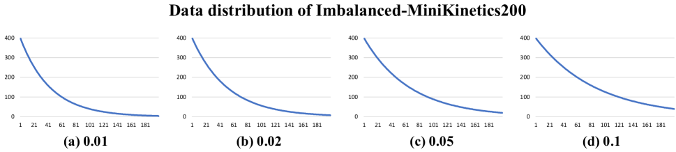
Figure 5: Data distribution according to varying imbalance ratios. (a), (b), (c), and (d) show the long-tailed distribution when the imbalance ratio is set to 0.01, 0.02, 0.05, and 0.1. The X-axis stands for video classes and Y-axis indicates the number of samples for each class.

10 Imbalanced-MiniKinetics200

In contrast to the potential in its practicality of Video long-tailed recognition, we found that the benchmark is limited to only one large-scale dataset, VideoLT. Particularly, the class frequency in the VideoLT dataset is shown to have linearity in logarithmic coordinate system (Zhang et al. 2021b) while other datasets collected from real applications may follow different data distribution. Therefore, we found a need for a new benchmarking dataset in which the data distribution can be adjusted to simulate various long-tailed data circumstances.

In this regard, we synthetically created the Imbalanced-MiniKinetics200 dataset to facilitate the research for video long-tailed recognition. To produce the Imbalanced-MiniKinetics200 dataset, videos belonging to each of 200 categories are sampled up to 400 videos from the Kinetics-400 dataset (Carreira and Zisserman 2017) as similarly as (Xie et al. 2018). Note that due to the unavailability of some videos in Kinetics-400 and the fact that not all videos are required to create an imbalanced dataset, not all 80,000 videos are downloaded. For details, we publicize the video list of downloaded videos in the code appendix. Class names are in the next paragraph in the sorted order from the head to the tail. Then, we used imbalance ratio $\mu$ to manipulate the harshness in imbalanced setting (Cui et al. 2019; Cao et al. 2019) by generating a imbalance vector $v\in(\mu,1)^{K}$ where K denotes the number of classes. Specifically, $v$ is multiplied class-wisely as $n_{i}=n_{max}v_{i}$ where $n_{i}$ and $n_{max}$ indicate number of samples for i-th class and the maximum number of videos in certain class. Depending on each scenario where imbalance ratio $\mu$ is set to different values in Tab. 4.1, we visualize how harsh long-tailed distribution is formed in Fig. 5.

In our github , we also provide instructions about the procedure to create the Imbalanced-MiniKinetics200 dataset. By following the instructions with specified video lists, the Imbalanced-MiniKinetics200 dataset can easily be downloaded. Training codes to train and evaluate various imbalanced scenarios are also available, while different scenarios can be easily designed by modifying the imbalance ratio.

Below, we enumerate the classes used for the Imbalanced-MiniKinetics200 in order from head to tail classes.

{ 0: ’beatboxing’, 1: ’finger snapping’, 2: ’air drumming’, 3: ’country line dancing’, 4: ’snatch weight lifting’, 5: ’high jump’, 6: ’cheerleading’, 7: ’deadlifting’, 8: ’spinning poi’, 9: ’bowling’, 10: ’lunge’, 11: ’passing American football (not in game)’, 12: ’dancing ballet’, 13: ’dancing macarena’, 14: ’gymnastics tumbling’, 15: ’shot put’, 16: ’kicking field goal’, 17: ’giving or receiving award’, 18: ’breakdancing’, 19: ’arm wrestling’, 20: ’headbanging’, 21: ’shaking head’, 22: ’golf driving’, 23: ’sticking tongue out’, 24: ’hurling (sport)’, 25: ’golf putting’, 26: ’catching or throwing baseball’, 27: ’blowing glass’, 28: ’brushing teeth’, 29: ’catching or throwing softball’, 30: ’front raises’, 31: ’bookbinding’, 32: ’eating spaghetti’, 33: ’clean and jerk’, 34: ’crawling baby’, 35: ’juggling balls’, 36: ’barbequing’, 37: ’bench pressing’, 38: ’flying kite’, 39: ’bungee jumping’, 40: ’feeding goats’, 41: ’side kick’, 42: ’contact juggling’, 43: ’milking cow’, 44: ’making snowman’, 45: ’eating ice cream’, 46: ’hitting baseball’, 47: ’somersaulting’, 48: ’capoeira’, 49: ’dribbling basketball’, 50: ’busking’, 51: ’dunking basketball’, 52: ’catching or throwing frisbee’, 53: ’blowing out candles’, 54: ’diving cliff’, 55: ’hammer throw’, 56: ’javelin throw’, 57: ’high kick’, 58: ’ice skating’, 59: ’brushing hair’, 60: ’cutting watermelon’, 61: ’hula hooping’, 62: ’dancing gangnam style’, 63: ’archery’, 64: ’abseiling’, 65: ’baking cookies’, 66: ’singing’, 67: ’driving tractor’, 68: ’curling hair’, 69: ’eating burger’, 70: ’long jump’, 71: ’smoking hookah’, 72: ’situp’, 73: ’folding napkins’, 74: ’cleaning floor’, 75: ’shuffling cards’, 76: ’jumping into pool’, 77: ’biking through snow’, 78: ’laughing’, 79: ’feeding birds’, 80: ’balloon blowing’, 81: ’belly dancing’, 82: ’ski jumping’, 83: ’cooking chicken’, 84: ’climbing tree’, 85: ’chopping wood’, 86: ’dying hair’, 87: ’driving car’, 88: ’feeding fish’, 89: ’canoeing or kayaking’, 90: ’sled dog racing’, 91: ’shoveling snow’, 92: ’doing nails’, 93: ’petting animal (not cat)’, 94: ’mowing lawn’, 95: ’crying’, 96: ’crossing river’, 97: ’opening present’, 98: ’smoking’, 99: ’shaving head’, 100: ’making pizza’, 101: ’folding paper’, 102: ’playing accordion’, 103: ’braiding hair’, 104: ’salsa dancing’, 105: ’jetskiing’, 106: ’shearing sheep’, 107: ’slacklining’, 108: ’filling eyebrows’, 109: ’sharpening pencil’, 110: ’playing badminton’, 111: ’picking fruit’, 112: ’passing American football (in game)’, 113: ’throwing discus’, 114: ’squat’, 115: ’ice climbing’, 116: ’skateboarding’, 117: ’massaging back’, 118: ’marching’, 119: ’surfing crowd’, 120: ’kitesurfing’, 121: ’spray painting’, 122: ’paragliding’, 123: ’playing bagpipes’, 124: ’parasailing’, 125: ’tap dancing’, 126: ’skiing (not slalom or crosscountry)’, 127: ’pole vault’, 128: ’playing basketball’, 129: ’presenting weather forecast’, 130: ’tai chi’, 131: ’playing ukulele’, 132: ’stretching leg’, 133: ’tobogganing’, 134: ’playing ice hockey’, 135: ’waxing chest’, 136: ’playing bass guitar’, 137: ’playing cricket’, 138: ’playing didgeridoo’, 139: ’riding elephant’, 140: ’motorcycling’, 141: ’playing cello’, 142: ’playing paintball’, 143: ’waxing legs’, 144: ’playing chess’, 145: ’robot dancing’, 146: ’playing poker’, 147: ’snowkiting’, 148: ’pull ups’, 149: ’playing recorder’, 150: ’playing xylophone’, 151: ’playing tennis’, 152: ’washing dishes’, 153: ’riding or walking with horse’, 154: ’playing volleyball’, 155: ’swimming breast stroke’, 156: ’playing clarinet’, 157: ’roller skating’, 158: ’reading book’, 159: ’playing violin’, 160: ’playing harmonica’, 161: ’playing saxophone’, 162: ’playing squash or racquetball’, 163: ’playing harp’, 164: ’tapping guitar’, 165: ’rock climbing’, 166: ’snowboarding’, 167: ’playing trumpet’, 168: ’throwing axe’, 169: ’washing feet’, 170: ’playing guitar’, 171: ’scrambling eggs’, 172: ’playing drums’, 173: ’swimming backstroke’, 174: ’riding unicycle’, 175: ’punching bag’, 176: ’walking the dog’, 177: ’surfing water’, 178: ’pushing car’, 179: ’snorkeling’, 180: ’trapezing’, 181: ’tango dancing’, 182: ’sailing’, 183: ’pushing cart’, 184: ’playing trombone’, 185: ’weaving basket’, 186: ’triple jump’, 187: ’pumping fist’, 188: ’washing hands’, 189: ’scuba diving’, 190: ’tying knot (not on a tie)’, 191: ’welding’, 192: ’water skiing’, 193: ’trimming or shaving beard’, 194: ’using computer’, 195: ’zumba’, 196: ’yoga’, 197: ’wrapping present’, 198: ’windsurfing’, 199: ’unboxing’ }

References

- Arandjelovic et al. (2016) Arandjelovic, R.; Gronat, P.; Torii, A.; Pajdla, T.; and Sivic, J. 2016. NetVLAD: CNN architecture for weakly supervised place recognition. In Proceedings of the IEEE conference on computer vision and pattern recognition, 5297–5307.
- Brattoli et al. (2020) Brattoli, B.; Tighe, J.; Zhdanov, F.; Perona, P.; and Chalupka, K. 2020. Rethinking zero-shot video classification: End-to-end training for realistic applications. In Proceedings of the IEEE/CVF Conference on Computer Vision and Pattern Recognition, 4613–4623.
- Buch et al. (2022) Buch, S.; Eyzaguirre, C.; Gaidon, A.; Wu, J.; Fei-Fei, L.; and Niebles, J. C. 2022. Revisiting the" Video" in Video-Language Understanding. In Proceedings of the IEEE/CVF Conference on Computer Vision and Pattern Recognition, 2917–2927.
- Buda, Maki, and Mazurowski (2018) Buda, M.; Maki, A.; and Mazurowski, M. A. 2018. A systematic study of the class imbalance problem in convolutional neural networks. Neural Networks, 106: 249–259.
- Cao et al. (2019) Cao, K.; Wei, C.; Gaidon, A.; Arechiga, N.; and Ma, T. 2019. Learning imbalanced datasets with label-distribution-aware margin loss. Advances in neural information processing systems, 32.
- Carreira and Zisserman (2017) Carreira, J.; and Zisserman, A. 2017. Quo vadis, action recognition? a new model and the kinetics dataset. In proceedings of the IEEE Conference on Computer Vision and Pattern Recognition, 6299–6308.
- Chapelle et al. (2000) Chapelle, O.; Weston, J.; Bottou, L.; and Vapnik, V. 2000. Vicinal risk minimization. Advances in neural information processing systems, 13.
- Chawla et al. (2002) Chawla, N. V.; Bowyer, K. W.; Hall, L. O.; and Kegelmeyer, W. P. 2002. SMOTE: synthetic minority over-sampling technique. Journal of artificial intelligence research, 16: 321–357.
- Choi et al. (2020) Choi, J.; Sharma, G.; Chandraker, M.; and Huang, J.-B. 2020. Unsupervised and semi-supervised domain adaptation for action recognition from drones. In Proceedings of the IEEE/CVF Winter Conference on Applications of Computer Vision.
- Chou et al. (2020) Chou, H.-P.; Chang, S.-C.; Pan, J.-Y.; Wei, W.; and Juan, D.-C. 2020. Remix: rebalanced mixup. In European Conference on Computer Vision, 95–110. Springer.
- Chu et al. (2020) Chu, P.; Bian, X.; Liu, S.; and Ling, H. 2020. Feature space augmentation for long-tailed data. In European Conference on Computer Vision, 694–710. Springer.
- Cui et al. (2019) Cui, Y.; Jia, M.; Lin, T.-Y.; Song, Y.; and Belongie, S. 2019. Class-balanced loss based on effective number of samples. In Proceedings of the IEEE/CVF conference on computer vision and pattern recognition, 9268–9277.
- Deng et al. (2009) Deng, J.; Dong, W.; Socher, R.; Li, L.-J.; Li, K.; and Fei-Fei, L. 2009. Imagenet: A large-scale hierarchical image database. In 2009 IEEE conference on computer vision and pattern recognition. Ieee.
- Dong, Gong, and Zhu (2017) Dong, Q.; Gong, S.; and Zhu, X. 2017. Class rectification hard mining for imbalanced deep learning. In Proceedings of the IEEE International Conference on Computer Vision, 1851–1860.
- Dosovitskiy et al. (2022) Dosovitskiy, A.; Beyer, L.; Kolesnikov, A.; Weissenborn, D.; Zhai, X.; Unterthiner, T.; Dehghani, M.; Minderer, M.; Heigold, G.; Gelly, S.; Uszkoreit, J.; and Houlsby, N. 2022. An Image is Worth 16x16 Words: Transformers for Image Recognition at Scale. In International Conference on Learning Representations.
- Fan et al. (2017) Fan, Y.; Lyu, S.; Ying, Y.; and Hu, B. 2017. Learning with average top-k loss. Advances in neural information processing systems, 30.
- Feng, Hong, and Zheng (2021) Feng, J.-C.; Hong, F.-T.; and Zheng, W.-S. 2021. Mist: Multiple instance self-training framework for video anomaly detection. In Proceedings of the IEEE/CVF Conference on Computer Vision and Pattern Recognition.
- He et al. (2016) He, K.; Zhang, X.; Ren, S.; and Sun, J. 2016. Deep residual learning for image recognition. In Proceedings of the IEEE conference on computer vision and pattern recognition, 770–778.
- Huang et al. (2016) Huang, C.; Li, Y.; Loy, C. C.; and Tang, X. 2016. Learning deep representation for imbalanced classification. In Proceedings of the IEEE conference on computer vision and pattern recognition, 5375–5384.
- Japkowicz and Stephen (2002) Japkowicz, N.; and Stephen, S. 2002. The class imbalance problem: A systematic study. Intelligent data analysis, 6(5): 429–449.
- Jégou et al. (2010) Jégou, H.; Douze, M.; Schmid, C.; and Pérez, P. 2010. Aggregating local descriptors into a compact image representation. In 2010 IEEE computer society conference on computer vision and pattern recognition, 3304–3311. IEEE.
- Kang et al. (2020) Kang, B.; Xie, S.; Rohrbach, M.; Yan, Z.; Gordo, A.; Feng, J.; and Kalantidis, Y. 2020. Decoupling Representation and Classifier for Long-Tailed Recognition. In International Conference on Learning Representations.
- Karakoulas and Shawe-Taylor (1998) Karakoulas, G.; and Shawe-Taylor, J. 1998. Optimizing classifers for imbalanced training sets. Advances in neural information processing systems, 11.
- Kim, Jeong, and Shin (2020) Kim, J.; Jeong, J.; and Shin, J. 2020. M2m: Imbalanced classification via major-to-minor translation. In Proceedings of the IEEE/CVF Conference on Computer Vision and Pattern Recognition, 13896–13905.
- Kubat, Matwin et al. (1997) Kubat, M.; Matwin, S.; et al. 1997. Addressing the curse of imbalanced training sets: one-sided selection. In Icml, volume 97, 179. Citeseer.
- Li, Cheung, and Lu (2021) Li, M.; Cheung, Y.-m.; and Lu, Y. 2021. Long-tailed Visual Recognition via Gaussian Clouded Logit Adjustment.
- Li et al. (2021) Li, S.; Gong, K.; Liu, C. H.; Wang, Y.; Qiao, F.; and Cheng, X. 2021. Metasaug: Meta semantic augmentation for long-tailed visual recognition. In Proceedings of the IEEE/CVF Conference on Computer Vision and Pattern Recognition, 5212–5221.
- Lin, Gan, and Han (2019) Lin, J.; Gan, C.; and Han, S. 2019. Tsm: Temporal shift module for efficient video understanding. In Proceedings of the IEEE/CVF International Conference on Computer Vision, 7083–7093.
- Lin et al. (2019) Lin, T.; Liu, X.; Li, X.; Ding, E.; and Wen, S. 2019. Bmn: Boundary-matching network for temporal action proposal generation. In Proceedings of the IEEE/CVF International Conference on Computer Vision, 3889–3898.
- Liu et al. (2020) Liu, J.; Sun, Y.; Han, C.; Dou, Z.; and Li, W. 2020. Deep representation learning on long-tailed data: A learnable embedding augmentation perspective. In Proceedings of the IEEE/CVF Conference on Computer Vision and Pattern Recognition, 2970–2979.
- Menon et al. (2020) Menon, A. K.; Jayasumana, S.; Rawat, A. S.; Jain, H.; Veit, A.; and Kumar, S. 2020. Long-tail learning via logit adjustment. International Conference on Learning Representations.
- Moon, Kim, and Heo (2022) Moon, W.; Kim, J.-H.; and Heo, J.-P. 2022. Tailoring Self-Supervision for Supervised Learning. In European Conference on Computer Vision, 346–364. Springer.
- More (2016) More, A. 2016. Survey of resampling techniques for improving classification performance in unbalanced datasets. arXiv preprint arXiv:1608.06048.
- Nam et al. (2020) Nam, J.; Cha, H.; Ahn, S.; Lee, J.; and Shin, J. 2020. Learning from failure: De-biasing classifier from biased classifier. Advances in Neural Information Processing Systems, 33: 20673–20684.
- Park and Kim (2022) Park, N.; and Kim, S. 2022. How Do Vision Transformers Work? In International Conference on Learning Representations.
- Park et al. (2021) Park, S.; Lim, J.; Jeon, Y.; and Choi, J. Y. 2021. Influence-balanced loss for imbalanced visual classification. In Proceedings of the IEEE/CVF International Conference on Computer Vision, 735–744.
- Ren et al. (2020) Ren, J.; Yu, C.; Ma, X.; Zhao, H.; Yi, S.; et al. 2020. Balanced meta-softmax for long-tailed visual recognition. Advances in Neural Information Processing Systems, 33: 4175–4186.
- Shen, Lin, and Huang (2016) Shen, L.; Lin, Z.; and Huang, Q. 2016. Relay backpropagation for effective learning of deep convolutional neural networks. In European conference on computer vision, 467–482. Springer.
- Shu et al. (2019) Shu, J.; Xie, Q.; Yi, L.; Zhao, Q.; Zhou, S.; Xu, Z.; and Meng, D. 2019. Meta-weight-net: Learning an explicit mapping for sample weighting. Advances in neural information processing systems, 32.
- Tan et al. (2020) Tan, J.; Wang, C.; Li, B.; Li, Q.; Ouyang, W.; Yin, C.; and Yan, J. 2020. Equalization loss for long-tailed object recognition. In Proceedings of the IEEE/CVF conference on computer vision and pattern recognition.
- Tang, Huang, and Zhang (2020) Tang, K.; Huang, J.; and Zhang, H. 2020. Long-tailed classification by keeping the good and removing the bad momentum causal effect. Advances in Neural Information Processing Systems.
- Thulasidasan et al. (2019) Thulasidasan, S.; Chennupati, G.; Bilmes, J. A.; Bhattacharya, T.; and Michalak, S. 2019. On mixup training: Improved calibration and predictive uncertainty for deep neural networks. Advances in Neural Information Processing Systems.
- Vaswani et al. (2017) Vaswani, A.; Shazeer, N.; Parmar, N.; Uszkoreit, J.; Jones, L.; Gomez, A. N.; Kaiser, Ł.; and Polosukhin, I. 2017. Attention is all you need. Advances in neural information processing systems, 30.
- Verma et al. (2019) Verma, V.; Lamb, A.; Beckham, C.; Najafi, A.; Mitliagkas, I.; Lopez-Paz, D.; and Bengio, Y. 2019. Manifold mixup: Better representations by interpolating hidden states. In International Conference on Machine Learning, 6438–6447. PMLR.
- Wang et al. (2022) Wang, C.; Gao, S.; Gao, C.; Wang, P.; Pei, W.; Pan, L.; and Xu, Z. 2022. Label-aware distribution calibration for long-tailed classification.
- Wang et al. (2021) Wang, X.; Lian, L.; Miao, Z.; Liu, Z.; and Yu, S. 2021. Long-tailed Recognition by Routing Diverse Distribution-Aware Experts. In International Conference on Learning Representations.
- Wang, Lyu, and Jing (2020) Wang, X.; Lyu, Y.; and Jing, L. 2020. Deep generative model for robust imbalance classification. In Proceedings of the IEEE/CVF Conference on Computer Vision and Pattern Recognition, 14124–14133.
- Wang, Ramanan, and Hebert (2017) Wang, Y.-X.; Ramanan, D.; and Hebert, M. 2017. Learning to model the tail. Advances in Neural Information Processing Systems, 30.
- Xie et al. (2018) Xie, S.; Sun, C.; Huang, J.; Tu, Z.; and Murphy, K. 2018. Rethinking spatiotemporal feature learning for video understanding. In European Conference on Computer Vision.
- Xu et al. (2020) Xu, M.; Zhao, C.; Rojas, D. S.; Thabet, A.; and Ghanem, B. 2020. G-tad: Sub-graph localization for temporal action detection. In Proceedings of the IEEE/CVF Conference on Computer Vision and Pattern Recognition, 10156–10165.
- Yang and Xu (2020) Yang, Y.; and Xu, Z. 2020. Rethinking the value of labels for improving class-imbalanced learning. Advances in neural information processing systems, 33: 19290–19301.
- Zhang et al. (2018) Zhang, H.; Cisse, M.; Dauphin, Y. N.; and Lopez-Paz, D. 2018. mixup: Beyond empirical risk minimization. In International Conference on Learning Representations.
- Zhang et al. (2021a) Zhang, S.; Li, Z.; Yan, S.; He, X.; and Sun, J. 2021a. Distribution alignment: A unified framework for long-tail visual recognition. In Proceedings of the IEEE/CVF Conference on Computer Vision and Pattern Recognition, 2361–2370.
- Zhang et al. (2021b) Zhang, X.; Wu, Z.; Weng, Z.; Fu, H.; Chen, J.; Jiang, Y.-G.; and Davis, L. S. 2021b. VideoLT: Large-scale Long-tailed Video Recognition. In Proceedings of the IEEE/CVF International Conference on Computer Vision, 7960–7969.
- Zhang et al. (2021c) Zhang, Y.; Hooi, B.; Hong, L.; and Feng, J. 2021c. Test-Agnostic Long-Tailed Recognition by Test-Time Aggregating Diverse Experts with Self-Supervision. arXiv preprint arXiv:2107.09249.
- Zhong et al. (2019) Zhong, J.-X.; Li, N.; Kong, W.; Liu, S.; Li, T. H.; and Li, G. 2019. Graph convolutional label noise cleaner: Train a plug-and-play action classifier for anomaly detection. In Proceedings of the IEEE/CVF Conference on Computer Vision and Pattern Recognition, 1237–1246.
- Zhong et al. (2021a) Zhong, Z.; Cui, J.; Liu, S.; and Jia, J. 2021a. Improving calibration for long-tailed recognition. In Proceedings of the IEEE/CVF Conference on Computer Vision and Pattern Recognition, 16489–16498.
- Zhong et al. (2021b) Zhong, Z.; Cui, J.; Liu, S.; and Jia, J. 2021b. Improving calibration for long-tailed recognition. In Proceedings of the IEEE/CVF conference on computer vision and pattern recognition.
- Zhu et al. (2022) Zhu, B.; Niu, Y.; Hua, X.-S.; and Zhang, H. 2022. Cross-Domain Empirical Risk Minimization for Unbiased Long-tailed Classification. In AAAI Conference on Artificial Intelligence.