Trace inequalities for Sobolev martingales
Abstract
We study limiting trace inequalities in the style of Maz’ya and Meyers–Ziemer for Sobolev martingales. We develop the Bellman function approach to such estimates, which allows to provide sufficient and almost necessary conditions on the martingale space and the martingale transform under which the trace inequalities hold true.
1 Introduction
The space of summable functions and its subspaces play a special role in analysis. Many statements that are true for spaces in the reflexive regime break at the endpoints; one may recall the boundedness of singular integrals as an example. Other remain true when interpreted properly, but the proofs might be more complicated. This is the instance for Sobolev embedding theorems. While the foundations of this theory in the reflexive regime were laid by Sobolev in [39], the endpoint case was not covered until the work of Gagliardo [12] and Nirenberg [26]. Even then, many natural interesting questions were left open in the case . One of the directions of research was initiated by Bourgain and Brezis in [5]. Roughly speaking, we may describe Bourgain–Brezis inequalities as
| (1.1) |
where is a differential operator of order or a Fourier multiplier with similar homogeneity properties, , and may satisfy additional constraints (such as ). Usually, these inequalities are related to vectorial behavior of the function or the operators in question ( is usually a vector field or a differential form). We refer the reader to the papers [4], [6], [7], [10], [15], [17], [18], [19], [20], [28], [29], [32], [33], [34], [35], [36], [41], [45], [46], among many others, as well as the surveys [37] and [40] for many Bourgain–Brezis inequalities.
There is a classical trace inequality
| (1.2) |
proved by Maz’ya in [22] and Meyers and Ziemer in [23] (see [21] for generalizations), which, seemingly does not have any relatives among Bourgain–Brezis inequalities. We call this inequality the trace inequality, because it allows to define traces of and even functions on sets of non-zero -measure (we plug for the natural Frostman measure related to the set). It is desirable to obtain similar inequalities in the generality of (1.1); first, because it is an inequality, which seems to be more difficult than the usual Bourgain–Brezis inequalities; second, such type inequalities often deliver information about geometric properties of corresponding -type measures. The depth of the desirable analog of (1.2) is emphasized by the fact that defining the trace on a hyperplane, the simplest -dimensional set, in the generality of (1.1) was already a demanding problem. We refer the reader to [8], [11], [13], and [14] for trace inequalities on hyperplanes for differential operators and -norms.
In this paper, we do not aim to say anything new about functions on . We wish to explore the aforementioned class of inequalities in the related martingale setting introduced in [3] (the discrete model might be traced to [16]). While there is a well-known analogy between singular integrals on and martingale transforms, the existence of an effect similar to that of Bourgain–Brezis inequalities in the martingale setting was noticed only in [3]. The consideration of these related discrete problems allows to guess the right way to prove statements in the Euclidean case. See [46] for the proof of several endpoint Bourgain–Brezis inequalities with the approach suggested by [3], [44] for a probabilistic model of weakly cancelling operators and the implementation of the reasoning of that paper on the Euclidean setting in [45]. See [43] for Maz’ya’s -inequalities in the martingale setting and [42] for the transference of that reasoning to the Euclidean setting.
In the forthcoming section, we introduce the martingale model. Section 3 contains description of our methods. In [3], the authors relied upon common combinatorial tricks for proving martingale inequalities (mostly stopping times), here we will need to use a finer tool called the Bellman function or the Burkholder method. We refer the reader to the foundational papers [9], [25] and the books [27], [49] for the basics of the Bellman function method. Though the present paper is self-contained, it might be instructive to consult [43], where a simpler Bellman function was used to solve a related problem. For smoothness of exposition, we first prove the non-limiting -trace inequality from [3] using Bellman function in Section 4. This is already interesting, because the Bellman extremal problem arising here seems new. Section 5 introduces additional requirements on the spaces and functionals and states the main result, Theorem 5.1. The assumptions we impose on the martingale Sobolev space (see Definition 5.1) might be thought of as martingale versions of the requirements that the -wave cone is empty introduced in [1] (see [47] as well). This is a simple condition on the operator as in (1.1) sufficient to conclude that any vectorial measure has the lower Hausdorff dimension at least ; note that in some cases this condition might be essentially sharpened, see [2]. Section 6 contains the proof of the main theorem, which has been reduced to a verification of a finite dimensional inequality by the Bellman function method in Section 4; the said finite dimensional inequalities are still non-trivial. The final section is devoted to two examples that emphasize the analogy between the martingale problems and similar questions in the Euclidean setting. We consider two particular cases of martingale Sobolev spaces that resemble the spaces and the space of divergence-free measures and apply our investigations to these two cases; the results are summarized in Theorems 7.1 and 7.2. We end the paper with formulating a conjecture about functions on the Euclidean space.
2 Sobolev martingales
Consider a probability space. If is a finite algebra of measurable sets, a non-empty set is called an atom provided there are no non-empty sets such that . Suppose that is a fixed natural number and is an -uniform filtration (i.e. an increasing sequence of set algebras, , such that each atom in is split into atoms in having equal masses; we also assume that is the trivial algebra) on the standard atomless probability space. The set of atoms of the algebra is denoted by . There is a natural tree structure on the set of all atoms : the atom is a kid of if . In such a case, is the parent of , and we denote the parent of by . For each atom , we enumerate its kids with the numbers and fix this enumeration.
We may treat our probability space equipped with an -uniform filtration as a metric space . The points of are infinite paths in the tree of atoms (we start from the whole space, then choose an atom in , then pass to one of its kids in , and so on). More formally, a path is a mapping . A point of that corresponds to such a mapping may be thought of as the intersection of the atoms , , where is the -th kid of . This allows to interpret atoms as subsets of . The distance between the two paths and is defined by the formula
With this metric, becomes a compact metric space. Another way to interpret is to identify a path with the formal series , which induces the surjection . This interpretation suggests to call the -th digit of . In this interpretation, the atoms become -adic subintervals of . One may prove that is homeomorphic to a Cantor-type set.
Recall that a sequence of random variables is called a martingale adapted to , provided, first, each is -measurable, and second, for any . For a martingale adapted to , let be the sequence of its martingale differences:
We refer the reader to Chapter VII in [38] for the general martingale theory. We will be working with a very narrow class of martingales adapted to uniform filtrations and will not use anything other than terminlogy from the general theory.
We will be using the notation to denote the integer interval with the endpoints and , including the endpoints. Consider the linear space
For each atom , the function attains at most values on , and, thus, might be identified with an element of . Namely, for any , we fix a bijective map
that maps the number to the -th kid of . This map may be extended linearly to the mapping between and the space of restrictions of all possible martingale differences to . This extended map is also called .
Let us observe that each signed Borel measure with bounded variation on generates a martingale via the formula
| (2.1) |
Note that the characteristic functions of atoms are continuous with respect to the metric and form a total family in the space (i.e. each measure on is uniquely defined by its values at the atoms). Using this fact one may establish the one-to-one correspondence via (2.1) between finite signed measures on and -martingales adapted to . By an martingale we mean a martingale such that is finite, the latter expression is the norm of .
The Hardy–Littlewood–Sobolev inequality for martingales (going back to [50]) reads as follows:
| (2.2) |
where and . Here and in what follows, the notation means , where the constant is uniform in a certain sense. For example, the constant in (2.2) should not depend on the particular choice of , however, it might depend on and . The parameter should be interpreted as the order of the integration operator. See [24] and [48] for more general versions of the Hardy–Littlewood–Sobolev inequality for martingales.
Remark 2.1.
Note that the inequality (2.2) is true when and since
| (2.3) |
If the martingale is -valued, then might be naturally identified with an element of (we apply to each of coordinates individually), here . In other words, we may think of the trace of on as of an matrix such that the sum of the elements in each row equals zero. Let be a linear subspace of . Consider the subspace of the -valued martingale space :
In view of (2.1), one should think of as of a -type space. These spaces were implicitly introduced in [16] and proved to be good discrete models for several problems in harmonic analysis on and the space of measures, see [3] and [44]; the former paper suggested the name ’Sobolev martingales’ since the behavior of the spaces resembles that of .
3 Setting of the trace problem and the Bellman function
Let be a linear operator and let . Consider the operator
| (3.1) |
This operator maps martingales to functions; by the correspondence (2.1), we may interpret it as an operator that transforms measures into functions (the series converges in with by Remark 2.1). The operator is used to make the formula mathematically rigorous, informally, (3.1) may be written as
| (3.2) |
We note that the operator cannot be applied to an arbitrary -valued martingale since is defined on only and the condition is required. We will also use the notation
| (3.3) |
Note that is -measurable. Therefore, is a martingale.
Remark 3.1.
Set . The choice of the identity operator for reduces to the martingale Riesz potential present in the Hardy–Littlewood–Sobolev inequality (2.2). A different choice of the operator might make the operator more cancelling than the Riesz potential (usually, larger are needed for such a choice). This is similar to the difference between the classical Euclidean Riesz potential and the kernel . As we will see, these additional cancellations become important only at endpoints (a similar effect appeared in [30]).
We will be studying the question: ’for which measures on does the inequality
| (3.4) |
hold true?’ This inequality allows to define -traces of on lower-dimensional subsets of (this explains the name ’trace inequlaity’). We will be working with simple martingales only since usually the result may be extended to the class of all -martingales by a routine limiting argument.
Definition 3.1.
We say that a measure with bounded variation on satisfies the Frostman condition provided
| (3.5) |
One may restate the Frostman conditions in terms of Morrey space norms, see [30]. Sometimes, the Frostman conditions is called the ball growth condition.
Remark 3.2.
One may prove that the -Frostman condition is necessary for (3.4), provided is not degenerate. Namely, assume that for any there exists such that the -th coordinate of as an element of , is non-zero (we will later denote this number by , ). Then, the -Frostman condition is necessary for (3.4). One may prove this by plugging ’elementary martingales’ into (3.4), i.e. martingales for which is non-zero for only single and single .
We will be working with a slightly more demanding ’bilinear’ form of (3.4):
| (3.6) |
Definition 3.2.
Define the Bellman function by the rule
| (3.7) |
The supremum in the formula above is taken over the set of simple martingales only; note that in such a case we may assume that is generated (via (2.1)) by a simple martingale as well.
The Bellman domain (i.e. the set of points for which the supremum in (3.7) is taken over a non-empty set) is
| (3.8) |
The Bellman function satisfies the boundary inequality (this follows from substitution of a constant martingale into (3.7))
| (3.9) |
The Bellman function also satisfies the main inequality
| (3.10) |
where
| (3.11) |
The symbol means the average, i.e. .
Proposition 3.3.
The Bellman function indeed satisfies the main inequality.
Proposition 3.3 is similar to Lemma in [43], so, we omit its proof. Formally, we will not needed. A reverse statement is more important for us. We need to set up notation before formulating it.
Definition 3.3.
Proposition 3.4.
A sequence of random variables is called a supermartingale provided each is -measurable (i.e. is adapted to ) and for any
| (3.16) |
If is a supermartingale, then
| (3.17) |
for any .
Proof of Proposition 3.4.
Let and let be its kids in . Let
| (3.18) |
By the martingale properties,
| (3.19) |
satisfy the splitting rules (3.11). In other words, the string formed by these numbers generated as above, belongs to the configuration space . Therefore, the main inequality (3.13) applies, which means exactly the supermartingale property
| (3.20) |
for the process (3.15); we have used the identity
| (3.21) |
∎
Corollary 3.5.
Proof.
By Definition 3.2, it suffices to prove the estimate
| (3.23) |
In fact, we will prove that on . Let and let be a pair of a simple martingale and a measure generated by a simple martingale that fulfills the requirements in (3.7) for these fixed . By Proposition 3.4, the corresponding process (3.15) is a supermartingale. Therefore,
| (3.24) |
for any . Let us pick sufficiently large (recall we are working with simple martingales). By the boundary inequality, the latter expression is bounded from below by
| (3.25) |
Since and are arbitrary, we get
| (3.26) |
which yields (3.23). ∎
Remark 3.6.
Definition 3.4.
The functions that satisfy the main inequality and the boundary inequality are usually called supersolutions.
4 Subcritical case
Let be a vector. Consider the function given by the formula
We may extend this function to by continuity. Then,
| (4.1) |
By Hölder’s inequality, this function is convex and non-increasing. If, in addition, for any , this function also satisfies . Consider yet another function :
| (4.2) |
The function is also convex, non-increasing, and satisfies . As an elementary computation shows,
| (4.3) |
We cite Theorem from [3] (there was no operator in [3]; the theorem below is not sensitive to ).
Theorem 4.1.
Let us give the Bellman function proof of this theorem (it relies upon the same principles as the original one in [3], but uses different language).
Theorem 4.2.
Assume (4.4). Then, for any sufficiently close to one, the function
| (4.5) |
is a supersolution, provided (depending on ).
The notation means the statement holds true when is sufficiently large and is also sufficiently large (depending on the particular choice of ). Note that Theorem 4.2 implies Theorem 4.1 via Corollary 3.5.
Definition 4.1.
If is a function, then its discrepancy is
| (4.6) |
The main inequality says that on .
Proof of Theorem 4.2.
We wish to prove
| (4.7) |
Let us first compute :
| (4.8) |
We see that this expression is always non-negative due to the splitting rules (3.11). What is more,
| (4.9) |
provided
| (4.10) |
for some fixed small (the notation means the Euclidean norm of ). Now we turn to the function and estimate its discrepancy. Let be such that , where . Then,
| (4.11) |
Thus, if
| (4.12) |
then , i.e., the discrepancy of the second term in (4.5) is non-negative. It was proved in Lemma of [3] that, given , for any there exists such that
| (4.13) |
provided (4.10) is violated. Therefore, if , is sufficiently close to one and is sufficiently small, then there exists a tiny such that
| (4.14) |
whenever and , which is slightly stronger than (4.12). Therefore,
| (4.15) |
provided (4.10) is violated with sufficiently small . We fix such an .
Combining (4.9), (4.15), and the simple estimate
| (4.16) |
we obtain
| (4.17) |
provided is sufficiently large (note that ). Indeed, in the case (4.10) holds true, (4.17) follows from (4.9) and (4.16) by the choice of sufficiently large ; in the case (4.10) is violated, we rely upon the positivity of and (4.15)111We will refer to this simple reasoning as to the flat/convex argument (see the explanation after the proof of the lemma)..
Thus, it remains to prove
| (4.18) |
This follows from direct computation
| (4.19) |
and the triangle inequality. ∎
Remark 4.1.
In [3], condition (4.10) played the pivotal role (see Definition in that paper). The atoms for which the corresponding quantities violated it were called -flat222The term ’flat’ symbolizes that the martingale develops along the flat part of the boundary of the ball of .. The core of the reasoning is contained in Lemma of [3], which manifests the principle that flat atoms (or flat configurations such that ) lie close to rank-one configurations. It is convenient to introduce the set of admissible -flat increments:
| (4.20) |
See [46] for ’translation’ of these notions into the language of the Euclidean space (instead of ). The following lemma justifies the heuristic principle that flat configurations are close to rank-one configurations.
Lemma 4.2.
Fix . Let be a neighborhood of the set
| (4.21) |
For sufficiently small , the violation of (4.10) together with the conditions and implies .
Proof.
Note that if violates (4.10) and , then for every (we assume is sufficiently small). Therefore, the configurations we consider are uniformly bounded as vectors in . Assume the contrary: for any there exists that does not belong to , , , and
| (4.22) |
Let be a limit point of the sequence . Then, , which means the triangle inequality turns into equality and there exist with , , such that . Since , we have . Therefore, belongs to (4.21), which contradicts the openness of . ∎
5 Additional requirements on and
Definition 5.1.
We call the space geometric if the corresponding function is affine.
The condition that a space is geometric is similar to the condition that the -wave cone is empty (see also Lemma 7.3 below); the latter condition played an important role in [1] and [47].
Proposition 5.1.
The space is geometric if there exists such that
-
1)
the inequality
(5.1) holds true for any vector ;
- 2)
Proof.
Let be a geometric space and let . Then, since is affine, we have . Thus, for arbitrary , we have for all , and, therefore,
| (5.3) |
Now let be the vector at which the infimum in (4.3) is attained (by compactness, such a vector exists). The inequality (5.3) turns into equality by the choice of . Thus, for any , equals either zero or . The set where it equals is the searched-for set ; it is clear that since has mean zero. ∎
Remark 5.2.
If is a geometric space, then is an integer.
Remark 5.3.
Proposition 5.1 may be reversed, the conditions described there are not only necessary, but also sufficient for to be a geometric space.
Definition 5.2.
Remark 5.4.
There might be several extremal vectors related to .
Remark 5.5.
The proof of Proposition 5.1 also says: if is a geometric space and for some , , then is an extremal vector for some . Indeed, by Jensen’s inequality444We use the weighted Jensen’s inequality for a concave function and substitute , , and .,
| (5.4) |
We know this inequality turns into equality. Thus, for each either or .
Definition 5.3.
Let be a geometric space. We say that an operator is canceling if the identity
| (5.5) |
holds true for any extremal vector and its support .
The following proposition resembles Theorem in [30].
Proposition 5.6.
Let be a geometric space. If (3.6) holds true at the endpoint , then is a canceling operator.
Proof.
Let be an extremal vector. Consider the martingale given by
| (5.6) |
In such a case, and . What is more,
| (5.7) |
Let be the support of . By (5.6), we have provided there is a digit in the -ary expansion of the ’number’ that does not belong to . Let us compute the values of at the other ’numbers’ :
| (5.8) |
Therefore, if we pick some large and consider the stopped martingale , then
| (5.9) |
at any point inside the set
| (5.10) |
The following two statements will contradict (3.6):
-
1)
(5.11) -
2)
the uniform probability measure on fulfills the -Frostman condition uniformly with respect to .
The second statement follows from the fact that the said measure is represented via the correspondence (2.1) by the martingale , which is the scalar version of , and the bound
| (5.12) |
To prove the first statement, we consider the random variables :
| (5.13) |
on the probability space equipped with the uniform probability measure. Note that these random variables are identically distributed and independent. We need to prove that as (note that the mathematical expectation is computed w.r.t the uniform measure on ). In the case , this follows from the triangle inequality. In the remaining case , we use the Central Limit Theorem
| (5.14) |
here is the variance of . Thus, . ∎
We will need yet another condition imposed on . The necessity of this condition is doubtable.
Definition 5.4.
Let be fixed. We say that a geometric space is non-local (of order ) if for any extremal vector supported on , any , and any the identity
| (5.15) |
implies that is proportional to .
In particular, the non-locality assumption implies that for any all such that there exists an extremal vector supported on , are proportional; this somehow resembles the strong cancellation condition in [14] (the similarity is emphasized by the Fourier-side sufficient condition of non-locality in Lemma 7.13 below). We are ready to formulate our main result — the endpoint trace theorem.
Theorem 5.1.
Let be a geometric non-local space and let be a canceling operator. Then, (3.6) holds true at the endpoint .
This theorem has a Bellman function behind it.
Theorem 5.2.
Let be a geometric non-local space and let be a canceling operator. There exists a collection of constants such that the function
| (5.16) |
is a supersolution.
Remark 5.7.
Mysteriosly, both terms and are required.
6 Proof of Theorem 5.2
In fact, the proof consists of an accurate computation and estimate of , which is done in several steps.
Estimates for .
One may verify that this function is a supersolution, provided is sufficiently large, using the reasonings presented in the proof of Theorem 4.2 (see (4.17)). Now we need to prove that this function is a supersolution with certain excess. We derive from (4.8) and (4.11) that
| (6.1) |
(recall ). By homogeneity with respect to the variables and , we may assume . We may also assume for sufficiently small , the other case will be covered by the flat/convex argument and the choice of large (or large for the initial function ). Thus, by Lemma 4.2, we need to study the behavior of the function
| (6.2) |
when lies in a neighborhood of some and lies in a neighborhood of . Using the homogeneity with respect to the variables and , we may assume and , which does not change the things much since all our functions are homogeneous of order one with respect to and . Of course, is not necessarily equal to anymore. Note that if is not an extremal vector, then
| (6.3) |
provided is sufficiently close to (since this function is positive at , see Remark 5.5). The case where is an extremal vector is covered by the following lemma.
Lemma 6.1.
Assume is an extremal vector of the geometric non-local space . If , is sufficiently close to , and is sufficiently close to , then
| (6.4) |
provided is sufficiently large; here .
Note that
| (6.5) |
where is the support of the extremal vector .
Proof.
By the reasonings above, it suffices to prove that
| (6.6) |
given the assumptions of the lemma. Let be the orthogonal projection onto the line spanned by . The notation means the negative part of the projection: it equals if and zero otherwise. Let be the support of . We expand the second term on the left hand side of (6.6) (see the proof of Lemma in [3] for similar estimates):
| (6.7) |
Let
| (6.8) |
which is equivalent to the distance between and . Then,
| (6.9) | ||||
| (6.10) | ||||
by our normalization . Therefore,
| (6.21) |
We use the identity (which follows from ) to rewrite the expression obtained in (6.21) as
| (6.22) |
Thus,
| (6.41) |
Claim: the assumption that is a non-local space (together with the normalization ) leads to the estimate
| (6.42) |
To prove the claim, consider the linear subspace of formed by the strings , where such that and ; here, as usual, . Note that the string formed of vectors when and when , belongs to this space. Therefore, it suffices to prove the inequality
| (6.51) |
Note that the function on the right hand side of this inequality is one-homogeneous and even. It suffices to prove this function is positive outside the origin. In such a case, it is a norm on , and the desired inequality (6.51) follows since any two norms on a finite dimensional space are equivalent. To prove
| (6.52) |
assume the contrary: let when for some non-zero . Since is a non-local space (see Definition 5.4), this means is proportional to . In particular, since some of the equals zero, is parallel to , which, by our assumption , means . Therefore, , a contradiction. Thus, we have proved the claim.
In particular, . Therefore, by (6.41), the estimate
| (6.53) |
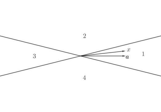
yields (6.6). Assume , then, without loss of generality, we may replace the with their projections onto the linear plane spanned by and (such a procedure will reduce the values in the formula above, while all the other quantities will remain the same). We will argue geometrically using Fig. 1. We split the plane spanned by and by the lines into four regions as it is drawn on Fig. 1.
If belongs to the second or the fourth domains, then (recall that is close to and, thus, lies strictly inside the first domain). If lies inside the first domain, then . Finally, in the third domain,
| (6.54) |
and thus, the choice of large implies
| (6.55) |
in this case, which proves (6.53) (in fact, we have proved the individual estimate
| (6.56) |
provided is sufficiently large). ∎
Estimates for .
Proposition 6.2.
For sufficiently large and the function
| (6.57) |
is a supersolution.
Proof.
We estimate
| (6.76) |
here we have used that for all (and also (6.1)). Similar to the proof of Theorem 4.2, by Lemma 4.2, it suffices to consider the case where is close to some and is close to (the other cases are covered by a combination of a compactness argument and the flat/convex argument). What is more, we may assume is an extremal vector (say, by (6.3)). Let be the support of . We normalize in such a way that and use Lemma 6.1 (or (6.6)):
| (6.77) |
Note that for the expression in the parenthesis is always non-negative since is close in this case, while is close to . Fix some . The function is Lipschitz on and vanishes at , which means its absolute value is bounded by
| (6.78) |
provided is sufficiently large (because the latter expression is the distance between and ).
Thus,
| (6.79) | |||
and the proof is completed by choosing large . ∎
End of proof of Theorem 5.2.
We rewrite the discrepancy of the first summand:
| (6.80) |
We will treat this expression as a function of and . Without loss of generality, we may assume and . The estimate
| (6.81) |
permits the application of the flat/convex argument, provided we have good estimates in neighborhoods of flat configurations, because if the configuration satisfies (4.10), then the discrepancy of the fourth term in (5.16) majorizes the discrepancies of the other three terms. We also note that the set of all -flat configurations is compact, provided we require the normalization . In particular, given any flat configuration , it suffices to find its neighborhood and a large constant such that
| (6.82) |
when lies inside the said neighborhood and , , and are arbitrary. If is not extremal, then the term
| (6.83) |
is bounded away from zero (uniformly with respect to and ) in a sufficiently small neighborhood of (say, by (6.3)), and the problem reduces to the choice of sufficiently large . Assume is extremal. As usual, we renormalize to . We estimate
| (6.84) |
this bound comes from (6.80) and the cancellation condition imposed on (for any we have ; recall also that given in (6.8) is the distance between and ). The second sum is compensated by the discrepancy of , by Lemma 6.1. As for the first sum, we have
| (6.85) |
provided is sufficiently close to . Thus, this part of the discrepancy may be compensated by by choosing sufficiently large .∎
7 Two examples
Let now , where and are natural numbers. We equip the set with the group structure of ; this also identifies it with the cube in a natural way. Let
| (7.1) |
be the generators of . It will be convenient to consider complex-valued functions and martingales, i.e. we set and identify and in a natural way. In our two main examples . The first example will model the space ,
| (7.2) |
The second will model the space of solenoidal charges,
| (7.3) |
Before we pass to the details, we survey simple facts about translation invariant spaces.
Definition 7.1.
We say that a linear subspace is translation invariant if for any and , the function also belongs to , the addition sign means addition in .
Note that the spaces and are translation invariant. Let us define the Fourier transform of a function by the formula
| (7.4) |
where is short for , and we interpret this expression as a residue modulo (a natural number in ). The inverse Fourier transform is then given by the formula
| (7.5) |
We refer the reader to the book [31] for introduction to abstract Fourier analysis (though our case of finite groups is elementary, sometimes the abstract intuition seems useful). The following lemma is simple, so, we leave it without proof.
Lemma 7.1.
The space is translation invariant if and only if there exist linear spaces , , such that
| (7.6) |
Remark 7.2.
Since any element of has mean zero, for any . We may set .
In the case , the corresponding spaces are complex lines defined by the formula
| (7.7) |
In the case the spaces are complex hyperplanes
| (7.8) |
If is a translation invariant space, the sets , where , play an important role:
| (7.9) |
since these sets contain the spectra of rank-one vectors. By spectrum of a function we mean the support of its Fourier transform.
Lemma 7.3.
Let . Assume that is a translation invariant subspace of such that
| (7.10) |
for any . Assume (7.10) turns into equality for at least one vector and that for this special we have , where is a subgroup of index in . Then, is a geometric space of order .
Proof.
Let be a rank-one vector. By definition,
| (7.11) |
Here we treat as a real valued function on . Therefore, whenever . Since , we have
| (7.12) |
Assume now that for any and let . Then, is supported in
| (7.13) |
and, since and the numbers are non-negative, for any . From this information and the bound (7.10), we conclude that
| (7.14) |
Therefore, by (4.1), . By convexity of the function and the identity ,
| (7.15) |
On the other hand, if the set
| (7.16) |
is a subgroup , then we set and see that for the corresponding . For such a choice of and , the inequalities (7.14) turn into equalities when , which means
| (7.17) |
and is the support of an extremal vector. Thus, the function is linear and is a geometric space. ∎
Remark 7.4.
The proof above says that extremal vectors correspond to those , for which the set
| (7.18) |
is a subgroup of index . If is an extremal vector, then its support is a coset of .
Definition 7.2.
A subset is called a combinatorial line generated by a set provided
| (7.19) |
Lemma 7.5.
Let . Then, for any , either
| (7.20) |
for some , or .
Proof.
Let . Assume some points belong to . By (7.7), this means there exist non-zero complex numbers such that
| (7.21) |
Define
| (7.22) |
Note that for any and . If there are at least two distinct non-zero values and , then the ratio
| (7.23) |
completely defines the elements and (i.e. these values do not depend on ) since the equation
| (7.24) |
has at most one solution when . Thus, either all non-zero are equal, or . In the latter case . In the former case, with given in (7.22). ∎
Corollary 7.6.
The space is a geometric space of order .
Proof.
We note that each combinatorial line is a subgroup of index and use Lemma 7.3. ∎
Remark 7.7.
The extremal vectors of are easy to describe: by Remark 7.4, each such vector is defined by its support, which is a coset of the subgroup , :
| (7.25) |
the corresponding vector is parallel to .
It is harder to describe the sets in general. We will only prove that apart from several exclusions, these sets are small provided is sufficiently large.
Lemma 7.8.
Let . Either , or
| (7.26) |
| (7.27) |
Remark 7.9.
The set (7.26) corresponds to being the -the basic vector in (or a multiple of it), the set (7.27) corresponds to being the difference of -th and -th basic vectors (or a mutliple of it). Using Remark 7.4, we may describe the extremal vectors. In the case (7.26), each such vector is supported by a coset of the subgroup
| (7.28) |
in other words, for any extremal vector of this type there exists such that it is supported by . In the case (7.27), the support of an extremal vector is a coset of the subgroup
| (7.29) |
The proof of Lemma 7.8 will take some time. We need an auxiliary lemma. Let . Consider the set
| (7.30) |
Lemma 7.10.
Let all , , be non-zero. If , then . In the case either or for some , , and in this case.
Proof.
Let us study the structure of the sets in the case first.
We rewrite the equation defining in the form
| (7.31) |
The left hand and right hand sides define two circles in the complex plane. In general, such two circles intersect by at most two points, which leads to the estimate . However, there is one exception: the two circles might coincide; in such a case, we cannot hope for anything better than (this estimate is definitely true). If the circles coincide, then and . Since we search for solutions , we also need , where , to have . We see that for any pair of non-zero numbers there exists at most one such that .
Now let us pass to the case and prove that in this case . We consider the sets
| (7.32) |
We note that since , for all but at most one values of (for this special value, we have ). Summing over all , we get .
Using induction and a similar ’slicing’ trick, we prove that for all larger . ∎
Proof of Lemma 7.8.
Remark 7.11.
We have proved that apart from the exceptions, , which is less than if .
Corollary 7.12.
For , the space is geometric of order .
Now we pass to verification of the non-locality condition given in Definition 5.4.
Lemma 7.13.
Let . Assume that is a translation invariant subspace of such that
| (7.35) |
for any . Assume also that if , where is a subgroup of index in , then for any coset of . Then, is a non-local space of order .
Proof.
By Remark 7.4 and translation invariance, it suffices to prove that if the function , where is a constant and , is supported in for some subgroup of index , , then is proportional to . If is supported in , then its Fourier transform is constant on each coset of . In particular, for any such coset and any ,
| (7.36) |
By (LABEL:parallelto0), is supported in and, by (LABEL:ParallelToa), is proportional to . Therefore, is proportional to . ∎
Corollary 7.14.
Let . The space is non-local of order and the space is non-local of order .
Proof.
Let now be an operator that commutes with translations. We may extend it to an operator mapping to and then average over translations. The resulting operator will be translation invariant. In particular, there exists a function such that
| (7.37) |
the symbol means the Fourier transform. Here we use scalar product in . Without loss of generality, we may assume (in case this relation does not hold for some , we may redefine to be the orthogonal projection of onto ; this will not change the formula (7.37)). In particular, . Using the inverse Fourier transform, we have
| (7.38) |
here . Assume now that satisfies the assumptions of Lemma 7.3. Let be an extremal vector. Then, by translation invariance and the condition , the cancellation condition from Definition 5.3 is equivalent to
| (7.39) |
here we assume is supported by a subgroup (see Remark 7.4). In the case , this reads as follows:
| (7.40) |
Theorem 7.1.
In the case , the cancellation condition turns into:
| (7.41) | |||
Theorem 7.2.
Compare with condition in [30] and Conjecture of the same paper. It says that the inequality
| (7.42) |
holds true for all measures satisfying the ball growth (or Frostman) condition , if and only if the kernel that is homogeneous of order satisfies the condition
| (7.43) |
for any .
Note that since the kernel is homogeneous of order , the latter condition may be informally interpreted that the (divergent) integral vanishes for any , which is somehow similar to (LABEL:CancellationDiv1) and (7.13). In a similar manner, Theorem 7.1 leads to another natural conjecture.
Conjecture 1.
Assume the kernel is homogeneous of order and smooth outside the origin. The inequality
| (7.44) |
holds true for all measures satisfying the condition if and only if for any
| (7.45) |
The integration is performed with respect to the natural Hausdorff measure on the -dimensional sphere .
References
- [1] A. Arroyo-Rabasa, G. De Philippis, J. Hirsch, and F. Rindler, Dimensional estimates and rectifiability for measures satisfying linear PDE constraints, Geom. Funct. Anal. 29 (2019), no. 3, 639–658.
- [2] R. Ayoush, On finite configurations in the spectra of singular measures, https://arxiv.org/2108.12036.
- [3] R. Ayoush, D. Stolyarov, and M. Wojciechowski, Sobolev martingales, Rev. Mat. Iberoam. 37 (2021), 1225–1246.
- [4] J. Bourgain and H. Brezis, On the equation and application to control of phases, J. Amer. Math. Soc. 16 (2003), no. 2, 393–426.
- [5] , New estimates for the Laplacian, the div–curl, and related Hodge systems, C. R. Math. Acad. Sci. Paris 338 (2004), 539–543.
- [6] , New estimates for elliptic equations and Hodge type systems, J. Eur. Math. Soc. 9 (2007), 277–315.
- [7] P. Bousquet and J. Van Schaftingen, Hardy–Sobolev inequalities for vector fields and canceling linear differential operators, Indiana Univ. Math. J. 63 (2014), no. 5, 1419–1445.
- [8] D. Breit, L. Diening, and F. Gmeineder, On the trace operator for functions of bounded -variation, Anal. & PDE 13 (2020), no. 2, 559–594.
- [9] D. L. Burkholder, Boundary value problems and sharp inequalities for martingale transforms, Ann. Prob. 12 (1984), no. 3, 647–702.
- [10] S. Chanillo, J. Van Schaftingen, and P.-L. Yung, Bourgain–Brezis inequalities on symmetric spaces of non-compact type, J. Funct. Anal. 273 (2017), no. 4, 1504–1547.
- [11] L. Diening and F. Gmeineder, Sharp trace and Korn inequalities for differential operators, https://arxiv.org/abs/2105.09570.
- [12] E. Gagliardo, Ulteriori proprieta di alcune classi di funzioni in piu variabili, Ric. Mat. 8 (1959), no. 1, 24–51, (in Italian).
- [13] F. Gmeineder, B. Raita, and J. Van Schaftingen, Boundary ellipticity and limiting -estimates on halfspaces, https://arxiv.org/2211.08167.
- [14] , On limiting trace inequalities for vectorial differential operators, Indiana Univ. Math. J. 70 (2021), no. 5, 2133–2176.
- [15] F. Hernandez and D. Spector, Fractional integration and optimal estimates for elliptic systems, https://arxiv.org/abs/2008.05639.
- [16] S. Janson, Characterizations of by singular integral transforms on martingales and , Math. Scand. 41 (1977), 140–152.
- [17] S. V. Kislyakov, D. V. Maximov, and D. M. Stolyarov, Differential expression with mixed homogeneity and spaces of smooth functions they generate in arbitrary dimension, J. Funct. Anal. 269 (2015), no. 10, 3220–3263.
- [18] L. Lanzani and E. M. Stein, A note on div curl inequalities, Math. Res. Let. 12 (2005), no. 1, 57–61.
- [19] V. Maz’ya, Bourgain–Brezis type inequality with explicit constants, Contemp. Math. 445 (2007), 247–252.
- [20] , Estimates for differential operators of vector analysis involving -norm, J. Eur. Math. Soc. 12 (2010), no. 1, 221–240.
- [21] , Sobolev spaces, Springer, 2011.
- [22] V. G. Maz’ya, The summability of functions belonging to Sobolev spaces, Problems of mathematical analysis, No. 5: Linear and nonlinear differential equations, Differential operators (Russian), 1975, pp. 66–98. MR 0511931
- [23] N. Meyers and W. Ziemer, Integral inequalities of Poincaré and Wirtinger type for BV functions, Amer. J. Math. 99 (1977), no. 6, 1345–1360. MR 507433
- [24] E. Nakai and G. Sadasue, Martingale Morrey–Campanato spaces and fractional integrals, J. Funct. Spaces Appl. (2012), Article ID 673929.
- [25] F. L. Nazarov and S. R. Treil, The hunt for a Bellman function: applications to estimates for singular integral operators and to other classical problems of harmonic analysis, Alg. i Anal. 8 (1996), no. 5, 32–162, translation in St. Petersburg Math. J. 8 (1997), no. 5, 721–824.
- [26] L. Nirenberg, On ellipltic partial differential equations, Ann. Scuola Norm. Sup Pisa 13 (1959), no. 3, 115–162.
- [27] A. Osȩkowski, Sharp martingale and semimartingale inequalities, Monografie Matematyczne IMPAN 72, Springer Basel, 2012.
- [28] B. Raita, -estimates for constant rank operators, arXiv:1811.10057.
- [29] , Critical -differentiability of -maps and canceling operators, Trans. Amer. Math. Soc. 372 (2019), no. 10, 7297–7326.
- [30] B. Raita, D. Spector, and D. Stolyarov, A trace inequality for solenoidal charges, Potential Anal. (2022).
- [31] W. Rudin, Fourier analysis on groups, Interscience Tracts in Pure and Applied Mathematics, No. 12, Interscience Publishers (a division of John Wiley & Sons, Inc.), New York-London, 1962. MR 0152834
- [32] J. Van Schaftingen, Estimates for -vector fields, C. R. Math. Acad. Sci. Paris 339 (2004), no. 3, 181–186.
- [33] , A simple proof of an inequality of Bourgain, Brezis and Mironescu, C. R. Math. Acad. Sci. Paris 338 (2004), no. 1, 23–26.
- [34] , Estimates for -vector fields under higher-order differential conditions, J. Eur. Math. Soc. 10 (2008), no. 4, 867–882.
- [35] , Limiting fractional and Lorentz space estimates of differential forms, Proc. Amer. Math. Soc. 138 (2010), 235–240.
- [36] , Limiting Sobolev inequalities for vector fields and canceling linear differential operators, J. Eur. Math. Soc. 15 (2013), no. 3, 877–921.
- [37] , Limiting Bourgain–Brezis estimates for systems of linear differential equations: theme and variations, J. Fixed Point Theory Appl. 15 (2014), no. 2, 273–297.
- [38] A. N. Shiryaev, Probability. 2, Graduate Texts in Mathematics, vol. 95, Springer, New York, 2019, Third edition of [ MR0737192], Translated from the 2007 fourth Russian edition by R. P. Boas and D. M. Chibisov.
- [39] S. Soboleff, Sur un théorème d’analyse fonctionnelle, Mat. Sbornik 4(46) (1938), no. 3, 471–497, (in Russian); translated in Amer. Math. Soc. Transl., 1963, 2(34), 39–68.
- [40] D. Spector, An optimal Sobolev embedding for , J. Funct. Anal. 279 (2020), no. 3, 108559.
- [41] D. Spector and J. Van Schaftingen, Optimal embeddings into Lorentz spaces for some vector differential operators via Gagliardo’s lemma, Atti Accad. Naz. Lincei Rend. Lincei Mat. Appl. 30 (2019), no. 3, 413–436.
- [42] D. Stolyarov, Fractional integration of summable functions: Maz’ya’s -inequalities, https://arxiv.org/abs/2109.08014.
- [43] , On -inequalities for martingale fractional integration and their Bellman functions, to appear in Michigan Math. J., https://arxiv.org/abs/2107.09336.
- [44] , Martingale interpretation of weakly cancelling differential operators, Zapiski Nauchn. Sem. POMI 480 (2019), 191–198, (in Russian); to be translated in J. Math. Sci. (N.Y.).
- [45] , Weakly canceling operators and singular integrals, Proc. Steklov Inst. Math. 312 (2021), 249–260.
- [46] , Hardy-Littlewood-Sobolev inequality for , Mat. Sb. 213 (2022), no. 6, 125–174.
- [47] , Dimension estimates for vectorial measures with restricted spectrum, J. Funct. Anal. 284 (2023), no. 1, 109735.
- [48] D. Stolyarov and D. Yarcev, Fractional integration for irregular martingales, Tohoku Math. J. (2) 74 (2022), no. 2, 253–261.
- [49] V. Vasyunin and A. Volberg, The Bellman function technique in Harmonic Analysis, Cambridge University Press, 2020.
- [50] C. Watari, Multipliers for Walsh–Fourier series, Tohoku Math. J. 16 (1964), no. 3, 239–251.
Dmitriy Stolyarov
St. Petersburg State University, 14th line 29B, Vasilyevsky Island, St. Petersburg, Russia.
d.m.stolyarov@spbu.ru.