Skewness consistency relation in large-scale structure and test of gravity theory

Abstract

We investigate the skewness of galaxy number density fluctuations as a possible probe to test gravity theories. We find that the specific linear combination of the skewness parameters corresponds to the coefficients of the second-order kernels of the density contrast, which can be regarded as the consistency relation and used as a test of general relativity and modified gravity theories. We also extend the analysis of the skewness parameters from real space to redshift space and derive the redshift-space skewness consistency relation.

I Introduction

It is one of the biggest challenges of modern cosmology to understand the physical origin of the present cosmic acceleration of the Universe. It might eventually require the presence of a new type of energy component, usually called dark energy. Another possibility is that the accelerated cosmic expansion could arise due to a modification of general relativity on cosmological scales. Among various cosmological observational data, measuring the growth history of density contrast of large-scale structure is one of the most popular tools to test the nature of dark energy and the modification of the theory of gravity responsible for the present cosmic acceleration. Although current observational data have already constrained the growth of structure at the linear level, there is no evidence of the deviation from the value predicted by the standard $\Lambda$ cold dark matter ($\Lambda$CDM) model. Hence, further investigation of the cosmological model landscape requires introducing other observables to capture the modification of gravity theory.

The power spectrum, or its Fourier counterpart, the two-point correlation function, is one of the most popular statistics to characterize cosmological observables such as cosmic microwave background and large-scale structure (e.g., Peebles book ). Since this can fully characterize the random Gaussian field, it can be treated as a good statistical quantity for large-scale structure on sufficiently large scales, or sufficiently early time, and cosmic microwave background. The cosmological structure generally grows nonlinearly in time due to gravitational interaction, which naturally introduces nonvanishing non-Gaussianity on small scale, or in late time, even in the case of the initial Gaussian field. Much information in such a non-Gaussian random field cannot be captured by solely using the power spectrum. A straightforward way to extract information on the non-Gaussianity of such a field is to consider higher-order spectra such as bispectrum, trispectrum, and so on (e.g., Bernardeau:2001qr ). However, it is challenging to measure these higher-order correlation functions accurately, since these are functions of scales with many arguments. Hence, it would be important to use other statistical tools for probing non-Gaussianities of random fields. The skewness, which is a measure of the asymmetry of the probability distribution of a random variable about its mean, is one of the popular measures to investigate the non-Gaussianity. The relation between higher-order spectra and the skewness parameters is derived analytically when the non-Gaussianity is weak Matsubara:1994wn ; Matsubara:2003yt . In particular, the leading order contributions of the higher-order spectra to the skewness parameters are determined through the integration of wavevectors of the bispectrum. Therefore, the skewness parameters can be used to extract the information of the bispectrum and higher-order spectra for the nonlinear density field.

In this paper, we consider the quasi-nonlinear growth of large-scale structure as a way to provide new insight into the modification of the gravity theory that would not be imprinted in the linear perturbation theory. It has been discussed in the literature that such a quasi-nonlinearity can be explored by observing the higher-order spectra of galaxies Takushima:2013foa ; Takushima:2015iha ; Yamauchi:2017ibz ; Hirano:2018uar ; Crisostomi:2019vhj ; Lewandowski:2019txi ; Hirano:2020dom ; Yamauchi:2021nxw and cosmic microwave background Namikawa:2018erh . In particular, a possible parameter to trace the nonlinear growth of structure is the time evolution of the coefficients of the second-order kernels for density contrast, the so-called second-order indices, which is originally developed in Ref. Yamauchi:2017ibz ; Namikawa:2018erh . However, Ref. Yamauchi:2021nxw pointed out that the features of the quasi-nonlinear growth are partially hidden by the uncertainty of the nonlinear galaxy bias functions. In order to extract the information of the modification of gravity theory obtained from the quasi-nonlinear growth, we need to carefully construct the combination of observables. In this paper, we focus on the skewness of the galaxy number density fluctuations as another probe of the underlying gravity theory. In particular, we use not only a common skewness parameter of the density field but also other skewness parameters which involve spatial derivatives of the density field. We investigate how the effects of the quasi-nonlinear growth appear in the skewness parameters and construct their combination of the skewness parameters that can be used to extract the information of the modification of gravity theory. Even in the case of the $\Lambda$CDM Universe with general relativity, the resultant expression represents the consistency relation between the skewness parameters.

This paper is organized as follows. In Sec.II, we summarize the skewness parameters derived in the previous works and develop the skewness parameters for the galaxy number density fluctuations as one of the actual observables of large-scale structure observations. We then derive the single consistency relation for the three real-space skewness parameters. In Sec. III, we extend the analysis to the redshift space, in which the effect of the anisotropic effect due to the redshift-space distortion should be properly included. We then derive the three consistency relations for the five independent redshift-space skewness parameters. Finally, Sec. IV is devoted to a summary and conclusion. Throughout this paper, as our fiducial model, we assume a $\Lambda$CDM cosmological model with parameters: $\Omega_{{\rm m},0}=0.3111$, $\Omega_{{\rm b},0}=0.0490$, $\Omega_{\Lambda}=0.6889$, $h=0.6766$, $A_{\rm s}=2.105\times 10^{-9}$, $n_{\rm s}=0.9665$, and $k_{\rm pivot}=0.05\,[{\rm Mpc}^{-1}]$.

II Skewness consistency relation in real space

In this section, we first summarize the description of the skewness parameters, following Matsubara:2003yt ; Matsubara:2020knr . We then calculate the skewness parameters from the bispectrum for the galaxy number density fluctuations, which includes the effects of the nonlinear gravitational clustering and galaxy biasing, as natural observables of large-scale structure observations. Combining the resultant expressions, we then derive a consistency relation of skewness parameters in real space.

II.1 Real-space skewness parameters

We consider three-dimensional density field $\rho({\bm{x}})$. We denote the density contrast by $\delta({\bm{x}})=\rho({\bm{x}})/\left\langle\rho({\bm{x}})\right\rangle-1$, where $\left\langle\cdots\right\rangle$ represents the ensemble average. We assume that the density contrast is smoothed by a smoothing function $W_{R}$ with smoothing length $R$, defined as

$$\delta_{R}({\bm{x}})=\int\mathrm{d}^{3}{\bm{x}}^{\prime}W_{R}(|{\bm{x}}-{\bm{x}}^{\prime}|)\delta({\bm{x}}^{\prime})\,.$$ (1)

In this paper, we use a Gaussian kernel function to obtain the smooth density field as

$$W_{R}(x)=\frac{e^{-x^{2}/(2R^{2})}}{(2\pi)^{3/2}R^{3}}\,.$$ (2)

The variance of density contrast smoothed on a scale $R$ is defined as

$$\sigma_{0}^{2}=\left\langle\delta_{R}^{2}\right\rangle\,.$$ (3)

Let us introduce the three real-space skewness parameters, which are defined as

$$S_{\rm r}^{(0)}=\frac{\left\langle\delta_{R}^{3}\right\rangle_{\rm c}}{\sigma_{0}^{4}}\,,$$ (4)

$$S_{\rm r}^{(1)}=\frac{3}{2}\frac{\left\langle\delta_{R}|\nabla\delta_{R}|^{2}\right\rangle_{\rm c}}{\sigma_{0}^{2}\sigma_{1}^{2}}\,,$$ (5)

$$S_{\rm r}^{(2)}=-\frac{9}{4}\frac{\left\langle|\nabla\delta_{R}|^{2}\Delta\delta_{R}\right\rangle_{\rm c}}{\sigma_{1}^{4}}\,,$$ (6)

where $\left\langle\cdots\right\rangle_{\rm c}$ denotes the three-point cumulants and we have defined $\sigma_{1}$ as

$$\sigma_{1}^{2}=\left\langle|\nabla\delta_{R}|^{2}\right\rangle\,.$$ (7)

To connect the statistical properties of the density contrast with the skewness parameters, it is convenient to consider the Fourier transform of the density field as

$$\widetilde{\delta}({\bm{k}})=\int\mathrm{d}^{3}{\bm{x}}e^{-i{\bm{k}}\cdot{\bm{x}}}\delta({\bm{x}})\,.$$ (8)

The Fourier transform of the smoothed density contrast is given by $\widetilde{\delta}_{R}({\bm{k}})=\widetilde{\delta}({\bm{k}})W(kR)$ , where $W(kR)$ denotes the Fourier transform of the kernel function $W_{R}(x)$ as $W(kR)=\int\mathrm{d}^{3}{\bm{x}}e^{-i{\bm{k}}\cdot{\bm{x}}}W_{R}(x)$. For the Gaussian smoothing, we have $W(kR)=e^{-k^{2}R^{2}/2}$. The power spectrum and bispectrum of the density contrast in the Fourier space have the forms

$$\left\langle\widetilde{\delta}({\bm{k}}_{1})\widetilde{\delta}({\bm{k}}_{2})\right\rangle=(2\pi)^{3}\delta_{\rm D}^{3}({\bm{k}}_{12})P(k_{1})\,,$$ (9)

$$\left\langle\widetilde{\delta}({\bm{k}}_{1})\widetilde{\delta}({\bm{k}}_{2})\widetilde{\delta}({\bm{k}}_{3})\right\rangle=(2\pi)^{3}\delta_{\rm D}^{3}({\bm{k}}_{123})B(k_{1},k_{2},k_{3})\,,$$ (10)

where ${\bm{k}}_{ij}={\bm{k}}_{i}+{\bm{k}}_{j}$, ${\bm{k}}_{ijk}={\bm{k}}_{i}+{\bm{k}}_{j}+{\bm{k}}_{k}$ . With these notations, the skewness parameters are written as Matsubara:2020knr

$$S_{\rm r}^{(a)}=\frac{1}{\sigma_{0}^{4-2a}\sigma_{1}^{2a}}\int\frac{\mathrm{d}^{3}{\bm{k}}_{1}}{(2\pi)^{3}}\frac{\mathrm{d}^{3}{\bm{k}}_{2}}{(2\pi)^{3}}\frac{\mathrm{d}^{3}{\bm{k}}_{3}}{(2\pi)^{3}}(2\pi)^{3}\delta_{\rm D}^{3}({\bm{k}}_{123})s^{(a)}({\bm{k}}_{1},{\bm{k}}_{2},{\bm{k}}_{3})B(k_{1},k_{2},k_{3})W(k_{1}R)W(k_{2}R)W(k_{3}R)\,,$$ (11)

where the kernel functions are given by

$$s^{(0)}=1\,,$$ (12)

$$s^{(1)}=-\frac{3}{2}{\bm{k}}_{1}\cdot{\bm{k}}_{2}\,,$$ (13)

$$s^{(2)}=-\frac{9}{4}({\bm{k}}_{1}\cdot{\bm{k}}_{2})k_{3}^{2}\,.$$ (14)

Thus, once the bispectrum for the density contrast is specified, we can calculate the skewness parameters by using the formula Eq. (11).

II.2 Reduced formula for real-space galaxy bispectrum

In the standard cosmological perturbation theory, gravitational nonlinear growth of structure gives non-negligible contributions to the nonlinear density field, which naturally leads to the non-vanishing bispectrum for the density field. Moreover, the density contrast is indirectly related to the observables of large-scale structure such as the galaxy number density fluctuations. Hence, it is natural to apply the formulation derived in the previous subsection to the bispectrum of the galaxy number density fluctuations, which includes the effects of the nonlinear gravitational clustering and the galaxy biasing. In the standard perturbation theory, the nonlinear density contrast in Fourier space, $\widetilde{\delta}({\bm{k}})$, is formally expanded in terms of the linear density contrast $\widetilde{\delta}_{\rm L}({\bm{k}})$ as

$$\widetilde{\delta}({\bm{k}})=\widetilde{\delta}_{\rm L}({\bm{k}})+\int\frac{\mathrm{d}^{3}{\bm{k}}_{1}}{(2\pi)^{3}}\frac{\mathrm{d}^{3}{\bm{k}}_{2}}{(2\pi)^{3}}(2\pi)^{3}\delta_{\rm D}^{3}({\bm{k}}_{12}-{\bm{k}})F_{2}({\bm{k}}_{1},{\bm{k}}_{2})\widetilde{\delta}_{\rm L}({\bm{k}}_{1})\widetilde{\delta}_{\rm L}({\bm{k}}_{2})+\cdots\,.$$ (15)

Here, the explicit form of the kernel function $F_{2}$ will be shown in the subsequent subsection. To connect the nonlinear density field $\delta$ with the galaxy number density fluctuations $\delta_{\rm g}$, we need some relation. We assume that the galaxy number density fluctuations $\delta_{\rm g}({\bm{x}})$ up to the second-order in the perturbative expansion of the density contrast $\delta({\bm{x}})$ is well described by the combination of the linear bias $b_{1}$, the second-order bias $b_{2}$, and the tidal bias $b_{K^{2}}$ as Desjacques:2016bnm

$$\delta_{\rm g}({\bm{x}})=b_{1}\delta({\bm{x}})+\frac{1}{2}b_{2}\Bigl{\{}[\delta({\bm{x}})]^{2}-\left\langle\delta^{2}\right\rangle\Bigr{\}}+b_{K^{2}}\Bigl{\{}[s_{ij}({\bm{x}})]^{2}-\left\langle s_{ij}^{2}\right\rangle\Bigr{\}}+\cdots\,,$$ (16)

where

$$s_{ij}=\left(\frac{\partial_{i}\partial_{j}}{\partial^{2}}-\frac{1}{3}\delta_{ij}\right)\delta(\bm{x})\,.$$ (17)

Here, the terms $\left\langle\delta^{2}\right\rangle$ and $\left\langle s_{ij}^{2}\right\rangle$ ensure the condition $\left\langle\delta_{\rm g}({\bm{x}})\right\rangle=0$. Combining these, the Fourier transform of the galaxy number density fluctuations $\widetilde{\delta}_{\rm g}({\bm{k}})$ in real space can be written in terms of the linear density contrast $\widetilde{\delta}_{\rm L}({\bm{k}})$:

$$\widetilde{\delta}_{\rm g}({\bm{k}})=b_{1}\widetilde{\delta}_{\rm L}({\bm{k}})+\int\frac{\mathrm{d}^{3}{\bm{k}}_{1}}{(2\pi)^{3}}\frac{\mathrm{d}^{3}{\bm{k}}_{2}}{(2\pi)^{3}}(2\pi)^{3}\delta_{\rm D}^{3}({\bm{k}}_{12}-{\bm{k}})Z_{2,{\rm r}}({\bm{k}}_{1},{\bm{k}}_{2})\widetilde{\delta}_{\rm L}({\bm{k}}_{1})\widetilde{\delta}_{\rm L}({\bm{k}}_{2})+\cdots\,.$$ (18)

where

$$Z_{2,{\rm r}}({\bm{k}}_{1},{\bm{k}}_{2}):=b_{1}F_{2}({\bm{k}}_{1},{\bm{k}}_{2})+\frac{1}{2}b_{2}+b_{K^{2}}\left\{(\widehat{\bm{k}}_{1}\cdot\widehat{\bm{k}}_{2})^{2}-\frac{1}{3}\right\}\,,$$ (19)

with $\widehat{\bm{k}}_{a}:={\bm{k}}_{a}/|{\bm{k}}_{a}|$. We now assume that the linear density contrast $\widetilde{\delta}_{\rm L}({\bm{k}})$ obeys the Gaussian statistics with the power spectrum $P_{\rm L}(k)$ defined through $\left\langle\widetilde{\delta}_{\rm L}({\bm{k}}_{1})\widetilde{\delta}_{\rm L}({\bm{k}}_{2})\right\rangle=(2\pi)^{3}\delta_{\rm D}^{3}({\bm{k}}_{12})P(k_{1})$. Hereafter, we consider the skewness parameters for the galaxy number density fluctuations instead of the density contrast since $\delta_{g}$ is the actual observable obtained from large-scale structure observations.

The power spectrum and bispectrum of galaxy number density fluctuations are defined as

$$\left\langle\widetilde{\delta}_{\rm g}({\bm{k}}_{1})\widetilde{\delta}_{\rm g}({\bm{k}}_{2})\right\rangle=(2\pi)^{3}\delta_{\rm D}^{3}({\bm{k}}_{12})P_{\rm g}(k_{1})\,,$$ (20)

$$\left\langle\widetilde{\delta}_{\rm g}({\bm{k}}_{1})\widetilde{\delta}_{\rm g}({\bm{k}}_{2})\widetilde{\delta}_{\rm g}({\bm{k}}_{3})\right\rangle=(2\pi)^{3}\delta_{\rm D}^{3}({\bm{k}}_{12})B_{\rm g}(k_{1},k_{2},k_{3})\,.$$ (21)

In the lowest-order approximation of the perturbation theory, the real-space galaxy bispectrum due to the nonlinear growth is given by

$$B_{\rm g,r}(k_{1},k_{2},k_{3})=2Z_{2,{\rm r}}({\bm{k}}_{1},{\bm{k}}_{2})b_{1}^{2}P_{\rm L}(k_{1})P_{\rm L}(k_{2})+\text{(cyc.)}\,,$$ (22)

where “$+({\rm cyc.})$” denotes the cyclic permutation with respect to the arguments ${\bm{k}}_{1}$, ${\bm{k}}_{2}$, and ${\bm{k}}_{3}$.

Let us evaluate the skewness parameters with the Gaussian smoothing kernel, following the method originally developed in Ref. Matsubara:1994wn . The galaxy skewness parameters we consider in this paper are given by

$$S_{\rm g,r}^{(0)}=\frac{\left\langle\delta_{\rm g}^{3}\right\rangle_{\rm c}}{\sigma_{{\rm g}0}^{4}}\,,$$ (23)

$$S_{\rm g,r}^{(1)}=\frac{3}{2}\frac{\left\langle\delta_{\rm g}|\nabla\delta_{\rm g}|^{2}\right\rangle_{\rm c}}{\sigma_{{\rm g}0}^{2}\sigma_{{\rm g}1}^{2}}\,,$$ (24)

$$S_{\rm g,r}^{(2)}=-\frac{9}{4}\frac{\left\langle|\nabla\delta_{\rm g}|^{2}\Delta\delta_{\rm g}\right\rangle_{\rm c}}{\sigma_{{\rm g}1}^{4}}\,,$$ (25)

where the quantities $\sigma_{{\rm g}j}$ for the galaxy number density fluctuations are given by

$$\sigma_{{\rm g}j}^{2}=b_{1}^{2}\int\mathrm{d}\ln k\,k^{2j}\frac{k^{3}}{2\pi^{2}}P_{\rm L}(k)W^{2}(kR)\,.$$ (26)

Using the expression of the galaxy bispectrum Eq. (22), we obtain the real-space galaxy skewness parameters as

$$S_{\rm g,r}^{(a)}=\frac{b_{1}^{2}}{\sigma_{{\rm g}0}^{4-2a}\sigma_{{\rm g}1}^{2a}}\int\frac{\mathrm{d}^{3}{\bm{k}}_{1}}{(2\pi)^{3}}\frac{\mathrm{d}^{3}{\bm{k}}_{2}}{(2\pi)^{3}}s^{(a)}({\bm{k}}_{1},{\bm{k}}_{2})\bigg{[}2Z_{2,{\rm r}}({\bm{k}}_{1},{\bm{k}}_{2})P_{\rm L}(k_{1})P_{\rm L}(k_{2})+({\rm cyc.})\biggr{]}e^{-(k_{1}^{2}+k_{2}^{2}+{\bm{k}}_{1}\cdot{\bm{k}}_{2})R^{2}}\,.$$ (27)

To evaluate the skewness parameters, it would be convenient to introduce the symmetrized kernel function $s^{(a),{\rm sym}}$ defined as

$$s^{(a),{\rm sym}}({\bm{k}}_{1},{\bm{k}}_{2},{\bm{k}}_{3}):=\frac{1}{3}s^{(a)}({\bm{k}}_{1},{\bm{k}}_{2},{\bm{k}}_{3})+(\text{cyc.})\,,$$ (28)

where $({\rm cyc.})$ denotes the cyclic permutations of the previous term. The explicit calculation shows

$$s^{(0),{\rm sym}}=1\,,$$ (29)

$$s^{(1),{\rm sym}}=\frac{1}{2}\left(k_{1}^{2}+k_{2}^{2}+{\bm{k}}_{1}\cdot{\bm{k}}_{2}\right)\,,$$ (30)

$$s^{(2),{\rm sym}}=\frac{3}{2}\Bigl{[}k_{1}^{2}k_{2}^{2}-({\bm{k}}_{1}\cdot{\bm{k}}_{2})^{2}\Bigr{]}\,.$$ (31)

Once we replace $s^{(a)}\to s^{(a),{\rm sym}}$ in Eq. (11), the bispectrum for the density contrast can be replaced by the following function:

$$S_{\rm g,r}^{(a)}=\frac{b_{1}^{2}}{\sigma_{{\rm g}0}^{4-2a}\sigma_{{\rm g}1}^{2a}}\int\frac{\mathrm{d}^{3}{\bm{k}}_{1}}{(2\pi)^{3}}\frac{\mathrm{d}^{3}{\bm{k}}_{2}}{(2\pi)^{3}}s^{(a),{\rm sym}}({\bm{k}}_{1},{\bm{k}}_{2})\,6Z_{2,{\rm r}}({\bm{k}}_{1},{\bm{k}}_{2})P_{\rm L}(k_{1})P_{\rm L}(k_{2})e^{-(k_{1}^{2}+k_{2}^{2}+{\bm{k}}_{1}\cdot{\bm{k}}_{2})R^{2}}\,.$$ (32)

By using the rotational invariance, we can reduce the dimensionality of the integrals for the skewness parameters. Introducing the coordinate system as

$${\bm{k}}_{1}=\frac{p}{R}\left(\sqrt{1-\nu^{2}},0,\nu\right)\,,\ \ \ {\bm{k}}_{2}=\frac{q}{R}\left(0,0,1\right)\,,$$ (33)

the integrals for the skewness parameters analytically reduce to

$$S_{\rm g,r}^{(a)}=\frac{b_{1}^{3}}{8\pi^{4}R^{2a+6}\sigma_{{\rm g}0}^{4-2a}\sigma_{{\rm g}1}^{2a}}\int_{0}^{\infty}\mathrm{d}p\int_{0}^{\infty}\mathrm{d}qe^{-(p^{2}+q^{2})}\widetilde{S}_{\rm g,r}^{(a)}(p,q)P_{\rm L}\left(\frac{p}{R}\right)P_{\rm L}\left(\frac{q}{R}\right)\,,$$ (34)

where $\widetilde{S}_{\rm g,r}^{(a)}(p,q)$ are kernel functions defined as

$$\widetilde{S}_{\rm g,r}^{(a)}(p,q)=\frac{6p^{2}q^{2}}{b_{1}}\int_{-1}^{1}\mathrm{d}\nu\widetilde{s}^{(a),{\rm sym}}(p,q,\nu)Z_{2,{\rm r}}(p,q,\nu)e^{-pq\nu}\,,$$ (35)

with

$$\widetilde{s}^{(0),{\rm sym}}=1\,,$$ (36)

$$\widetilde{s}^{(1),{\rm sym}}=\frac{1}{2}\left(p^{2}+q^{2}+pq\nu\right)\,,$$ (37)

$$\widetilde{s}^{(2),{\rm sym}}=\frac{3p^{2}q^{2}}{2}\left(1-\nu^{2}\right)\,.$$ (38)

Therefore, once the explicit expression of the second-order kernel of the density contrast, $F_{2}$, is given, we evaluate the skewness parameters by integrating the above formula.

II.3 Consistency relation in real space

To proceed the analysis, let us consider the specific type of the second-order kernel of the density contrast, $F_{2}$. In this paper, we will consider the following form Takushima:2013foa ; Takushima:2015iha ; Yamauchi:2017ibz ; Hirano:2018uar ; Crisostomi:2019vhj ; Lewandowski:2019txi ; Hirano:2020dom ; Yamauchi:2021nxw :

$$F_{2}({\bm{k}}_{1},{\bm{k}}_{2})=\kappa\biggl{[}1+\frac{1}{2}(\widehat{\bm{k}}_{1}\cdot\widehat{\bm{k}}_{2})\left(\frac{k_{1}}{k_{2}}+\frac{k_{2}}{k_{1}}\right)\biggr{]}-\frac{2}{7}\lambda\biggl{[}1-(\widehat{\bm{k}}_{1}\cdot\widehat{\bm{k}}_{2})^{2}\biggr{]}\,,$$ (39)

where $\kappa$ and $\lambda$ are time-dependent parameters corresponding to the coefficients for the terms with characteristic wavevector dependence and they depend on the underlying gravity theory. It is known that this specific form of the second-order kernels describes a wide variety of the modified theory of gravity since the modification of gravity theory alters the clustering properties of nonlinear structures. In the Einstein-de Sitter Universe with general relativity, one finds $\kappa=\lambda=1$ Takushima:2013foa , while in the case of the $\Lambda$CDM Universe, $\lambda$ slightly deviates from unity. In the limit of $\Omega_{\rm m}\approx 1$, $\lambda$ can be well approximated as $\lambda\approx 1-\frac{3}{572}(1-\Omega_{\rm m})$ Yamauchi:2017ibz ; Bouchet:1994xp ; Bernardeau:2001qr . If the gravity theory is described by the Horndeski scalar-tensor gravity theories Horndeski:1974wa ; Deffayet:2011gz ; Kobayashi:2011nu , $\kappa$ still takes the standard value, but the deviation of $\lambda$ from unity contains the information from the underlying gravity model Takushima:2013foa ; Yamauchi:2017ibz . In the case of a broader class of scalar-tensor gravity theories called degenerate higher-order scalar-tensor (DHOST) theories Langlois:2015cwa ; Crisostomi:2016czh ; Achour:2016rkg ; BenAchour:2016fzp ; Langlois:2017dyl (see Langlois:2018dxi ; Kobayashi:2019hrl for a review) which is a natural extension of the Horndeski theory, both $\kappa$ and $\lambda$ can depend on time and deviate from unity Hirano:2018uar ; Crisostomi:2019vhj ; Lewandowski:2019txi ; Hirano:2020dom ; Yamauchi:2021nxw . Therefore, the time dependence of the coefficients of the second-order kernel, namely $\kappa$ and $\lambda$, yields a powerful probe of modified gravity theories. Hereafter, we consider how we can extract the information of $\kappa$ and $\lambda$ from observations of the skewness parameters.

In order to evaluate the skewness parameters in this setup, we substitute Eq. (39) into Eq. (19) with the coordinate of Eq. (33) to obtain the real-space $Z_{2}$ kernel as

$$\frac{2}{b_{1}}Z_{2,{\rm r}}(p,q,\nu)=g_{0}\mathsf{P}_{0}+g_{1}\mathsf{P}_{1}+g_{2}\mathsf{P}_{2}\,,$$ (40)

where

$$\mathsf{P}_{0}=P_{0}(\nu)\,,\ \ \mathsf{P}_{1}=\left(\frac{p}{q}+\frac{q}{p}\right)P_{1}(\nu)\,,\ \ \mathsf{P}_{2}=P_{2}(\nu)\,,$$ (41)

with $P_{i}(\nu)$ being the Legendre polynomials. Here, we have introduced $g_{i}$ ($i=0,1,2$), which are written in terms of $\kappa$, $\lambda$, and the bias functions as

$$g_{0}=2\kappa-\frac{8}{21}\lambda+\frac{b_{2}}{b_{1}}\,,$$ (42)

$$g_{1}=\kappa\,,$$ (43)

$$g_{2}=\frac{4}{3}\left(\frac{2}{7}\lambda+\frac{b_{K^{2}}}{b_{1}}\right)\,.$$ (44)

In the case of the Einstein-de Sitter Universe without introducing the nonlinear bias factors, these are written as $g_{0}=34/21,g_{1}=1$, and $g_{2}=8/21$. The kernel functions given in Eq. (35) reduce to

$$\widetilde{S}_{\rm g,r}^{(0)}=-6\Bigl{[}g_{1}(p^{2}+q^{2})+3g_{2}\Bigr{]}\left(\cosh(pq)-\frac{\sinh(pq)}{pq}\right)+6(g_{0}+g_{2})pq\sinh(pq)\,,$$ (45)

$$\widetilde{S}^{(1)}_{\rm g,r}=-3\Bigl{[}g_{0}p^{2}q^{2}+g_{1}(p^{2}+q^{2})(2+p^{2}+q^{2})+g_{2}(3+p^{2})(3+q^{2})\Bigr{]}\left(\cosh(pq)-\frac{\sinh(pq)}{pq}\right)$$

$$\qquad\qquad+3\Bigl{[}g_{0}(p^{2}+q^{2})+g_{1}(p^{2}+q^{2})+g_{2}(3+p^{2}+q^{2})\Bigr{]}pq\sinh(pq)\,,$$ (46)

$$\widetilde{S}^{(2)}_{\rm g,r}=18\Bigl{[}g_{0}p^{2}q^{2}+3g_{1}(p^{2}+q^{2})+(18+p^{2}q^{2})g_{2}\Bigr{]}\left(\cosh(pq)-\frac{\sinh(pq)}{pq}\right)-18\Bigl{[}g_{1}(p^{2}+q^{2})+6g_{2}\Bigr{]}pq\sinh(pq)\,.$$ (47)

When substituting $g_{0}=34/21,g_{1}=1$, and $g_{2}=8/21$ into the above expressions, one can easily reproduce the results derived in Matsubara:2020knr . An important observation is that all the parameters $g_{i}$ linearly appear in the above expression of the skewness parameters. Therefore, $g_{i}$ can be rewritten in terms of the linear combination of the skewness parameters. To do so, it would be convenient to introduce the matrix $\mathsf{M}_{\rm r}$, whose components are given by

$$\mathsf{M}_{\rm r}^{(a)}{}_{(i)}:=\frac{\partial S_{\rm g,r}^{(a)}}{\partial g_{i}}=\frac{b_{1}^{3}}{8\pi^{4}R^{2a+6}\sigma_{0}^{4-2a}\sigma_{1}^{2a}}\int_{0}^{\infty}\mathrm{d}p\int_{0}^{\infty}\mathrm{d}qe^{-(p^{2}+q^{2})}\widetilde{\mathsf{M}}_{\rm r}^{(a)}{}_{(i)}(p,q)P_{\rm L}\left(\frac{p}{R}\right)P_{\rm L}\left(\frac{q}{R}\right)\,.$$ (48)

Here one can easily extract the explicit form of $\widetilde{\mathsf{M}}_{\rm r}^{(a)}{}_{(i)}(p,q):=\partial\widetilde{S}_{\rm r}^{(a)}(p,q)/\partial g_{i}$ from Eqs. (45)–(47). Once the shape of the linear power spectrum $P_{\rm L}(k)$ is given, the matrix components can be obtained by integrating Eq. (48) numerically. With this convention, the set of three equations for the skewness parameters can be rewritten in a simpler form

$$S_{\rm g,r}^{(a)}=\sum_{i=0}^{2}\mathsf{M}_{\rm r}^{(a)}{}_{(i)}\,g_{i}\,.$$ (49)

At least in the standard cosmology with our fiducial parameter set, it is numerically confirmed that the determinant of $\mathsf{M}$ is nonzero. We therefore solve the above equation in terms of $g_{i}$ as

$$g_{i}=\sum_{a=0}^{2}\,[\mathsf{M}_{\rm r}^{-1}]^{(i)}{}_{(a)}S_{\rm g,r}^{(a)}\,.$$ (50)

This is one of the main results of this paper. However, $\kappa$ and $\lambda$ always appear with the nonlinear galaxy bias function in $g_{0}$ and $g_{2}$ terms, as seen in Eqs. (42) and (44), which indicates that there is a strong degeneracy between $\kappa$, $\lambda$, $b_{2}$, and $b_{K^{2}}$. The signals of gravity theory existing in $g_{0}$ and $g_{2}$ terms would be hidden by the uncertainty of the nonlinear bias factors. Therefore, the meaningful consistency relation comes only from $g_{1}$ term:

$$g_{1}=\kappa=[\mathsf{M}_{\rm r}^{-1}]^{(1)}{}_{(0)}S_{\rm g,r}^{(0)}+[\mathsf{M}_{\rm r}^{-1}]^{(1)}{}_{(1)}S_{\rm g,r}^{(1)}+[\mathsf{M}_{\rm r}^{-1}]^{(1)}{}_{(2)}S_{\rm g,r}^{(2)}\,.$$ (51)

As discussed above, the confirmation of the deviation of $g_{1}=\kappa$ from unity would indicate a departure from the Einstein gravity, in particular, the specific types of the modification of gravity theory, the DHOST theory beyond-Horndeski class Hirano:2018uar ; Crisostomi:2019vhj ; Lewandowski:2019txi ; Hirano:2020dom ; Yamauchi:2021nxw , which can be tested once we measure the skewness parameters. On the other hand, when gravity is described by the Horndeski scalar-tensor theory including general relativity, we have $g_{1}=\kappa=1$, therefore Eq. (51) can be regarded as the consistency relation among the three skewness parameters in the theory.

Figure 1: The absolute value of the coefficients appearing in the consistency relation for the real-space skewness parameters, $[\mathsf{M}_{\rm r}^{-1}]^{(1)}{}_{(a)}/b_{1}$, as a function of the smoothing length $R\,[h^{-1}{\rm Mpc}]$ with $a=0$ (red solid), $a=1$ (blue dot-dashed), and $a=2$ (green dashed).

Before closing this section, as a demonstration, we show the consistency relation for the real-space skewness parameters Eq. (51) with explicit numerical coefficients for a given smoothing scale. To calculate it explicitly, we need to specify the statistical nature of the linear density field. The linear density field $\delta_{\rm L}$ is related to the primordial curvature perturbation $\Phi$ through

$$\delta_{\rm L}({\bm{k}})={\cal M}(k)\Phi({\bm{k}})\,,$$ (52)

where the function ${\cal M}(k)$ is defined as

$${\cal M}(k,z)=\frac{2}{3}\frac{D_{+}(z)}{D_{+}(z_{\ast})(1+z_{\ast})}\frac{k^{2}T(k)}{H_{0}^{2}\Omega_{\rm m,0}}\,,$$ (53)

with $D_{+}(z)$ being the linear growth rate, and $z_{\ast}$ represents an arbitrary redshift at the matter-dominated era. $T(k)$ is the matter transfer function normalized to unity on large scales Eisenstein:1997ik . The power spectrum for the linear density field is related to that of the primordial perturbations as $P_{\rm L}(k)={\cal M}^{2}(k)P_{\Phi}(k)$, where $P_{\Phi}(k)$ denotes the power spectrum for the primordial curvature perturbations. With these, we now calculate the matrix components of $\mathsf{M}_{\rm r}$ and the corresponding consistency relation:

$$\mathsf{M}_{\rm r}=\frac{1}{b_{1}}\left(\begin{array}[]{ccc}3.4930&-2.1752&0.21206\\ 3.4049&-1.9486&0.17288\\ 4.2484&-3.0878&-0.34998\\ \end{array}\right)\,,$$ (57)

$$\frac{1}{b_{1}}\kappa=-4.621S_{\rm g,r}^{(0)}+5.094S_{\rm g,r}^{(1)}-0.283S_{\rm g,r}^{(2)}\,,$$ (58)

for $R=10\,h^{-1}{\rm Mpc}$, and

$$\mathsf{M}_{\rm r}=\frac{1}{b_{1}}\left(\begin{array}[]{ccc}3.9437&-3.2262&0.41878\\ 3.8551&-3.0347&0.37766\\ 4.9700&-4.2711&-0.17060\\ \end{array}\right)\,,$$ (62)

$$\frac{1}{b_{1}}\kappa=-7.168S_{\rm g,r}^{(0)}+7.789S_{\rm g,r}^{(1)}-0.354S_{\rm g,r}^{(2)}\,,$$ (63)

for $R=30\,h^{-1}{\rm Mpc}$. We show in Fig. 1 the coefficients of the consistency relation for the real-space skewness parameters, namely $|[\mathsf{M}_{\rm r}^{-1}]^{(1)}{}_{(a)}|/b_{1}$ with $a=0$ (red solid), $a=1$ (blue dot-dashed), and $a=2$ (green dashed), as a function of the smoothing length $R\,[h^{-1}{\rm Mpc}]$. This implies that the contribution from $S_{\rm g,r}^{(2)}$ is suppressed by an order of magnitude compared to the other two contributions, while the other two are of the same order of magnitude. Therefore, $S^{(0)}_{\rm g,r}$ and $S^{(1)}_{\rm g,r}$ would essentially determine the consistency relation.

Before closing this section, we would like to comment on the scales for which these consistency conditions are valid. In Ref. Matsubara:2020knr , the authors showed that the skewness parameters in the $N$-body simulations, which can probe fully nonlinear regime, are qualitatively reproduced by the tree-level perturbation theory on large scales within 5$\%$ precision level for $R\gtrsim 30\,h^{-1}{\rm Mpc}$, while its accuracy decreases to more than 10$\%$ for $R\lesssim 20\,h^{-1}{\rm Mpc}$. Therefore, in the case of the small smoothing length, e.g., $R\lesssim 10\,h^{-1}{\rm Mpc}$, the nonlinear corrections are needed in the analytic formula.

III Skewness consistency relation in redshift space

In redshift space, the radial position of galaxies is given by the observed radial component of its relative velocity to an observer. The peculiar velocity field of the underlying matter density, ${\bm{v}}$, distorts the observed position of the galaxy along the line of sight. The mapping of a galaxy from its position ${\bm{x}}$ in real space to its position ${\bm{s}}$ in redshift space along the line-of-sight direction ${\bm{n}}$ is expressed as

$${\bm{s}}({\bm{x}})={\bm{x}}+\frac{{\bm{v}}\cdot{\bm{n}}}{aH}{\bm{n}}\,.$$ (64)

Hence, in redshift space, the density contrast should be treated as a statistically anisotropic quantity. Even in the presence of anisotropy in the direction along the line of sight, all statistical measures should be independent with respect to sky rotations in the plane perpendicular to the line of sight. We will consider the skewness parameters in the plane-parallel approximation.

III.1 Skewness parameters in redshift space

To take into account the effect of redshift-space distortions, we need to treat the line-of-sight and the perpendicular directions separately. Hence, it is obvious that there are other independent parameters of skewness in anisotropic redshift space (see Codis:2013exa for similar quantities). In this subsection, we would like to derive the redshift-space skewness parameters describing the statistically anisotropic quantities. In redshift space, we have several possibilities for the skewness parameters, e.g.,

$$\frac{3}{2}\frac{\left\langle\delta_{\rm g}|\nabla_{\parallel}\delta_{\rm g}|^{2}\right\rangle_{\rm c}}{\sigma_{{\rm g}0}^{2}\sigma_{{\rm g}\parallel}^{2}}\,,\ \ \ \frac{3}{2}\frac{\left\langle\delta_{\rm g}|\nabla_{\perp}\delta_{\rm g}|^{2}\right\rangle_{\rm c}}{\sigma_{{\rm g}0}^{2}\sigma_{{\rm g}\perp}^{2}}\,,$$ (65)

for the extension of $S^{(1)}$,

$$-\frac{9}{4}\frac{\left\langle|\nabla_{\parallel}\delta_{\rm g}|^{2}\Delta_{\parallel}\delta_{\rm g}\right\rangle_{\rm c}}{\sigma_{{\rm g}\parallel}^{4}}\,,\ \ \ -\frac{9}{4}\frac{\left\langle|\nabla_{\perp}\delta_{\rm g}|^{2}\Delta_{\perp}\delta_{\rm g}\right\rangle_{\rm c}}{\sigma_{{\rm g}\perp}^{4}}\,,\ \ \ -\frac{9}{4}\frac{\left\langle|\nabla_{\perp}\delta_{\rm g}|^{2}\Delta_{\parallel}\delta_{\rm g}\right\rangle_{\rm c}}{\sigma_{{\rm g}\perp}^{2}\sigma_{{\rm g}\parallel}^{2}}\,,\ \ \ -\frac{9}{4}\frac{\left\langle|\nabla_{\parallel}\delta_{\rm g}|^{2}\Delta_{\perp}\delta_{\rm g}\right\rangle_{\rm c}}{\sigma_{{\rm g}\parallel}^{2}\sigma_{{\rm g}\perp}^{2}}\,,$$ (66)

for the extension of $S^{(2)}$, where we have introduced

$$\sigma_{{\rm g}\parallel}^{2}=\left\langle|\nabla_{\parallel}\delta_{\rm g}|^{2}\right\rangle\,,$$ (67)

$$\sigma_{{\rm g}\perp}^{2}=\left\langle|\nabla_{\perp}\delta_{\rm g}|^{2}\right\rangle\,.$$ (68)

However, as shown below, some of these possibilities are not independent. To construct the independent set of the anisotropic skewness parameters, we first develop the trial function and check its behavior. Based on this consideration, let us consider the trial functional form of the skewness parameter for the anisotropic bispectrum as

$$S^{(a),{\rm trial}}_{\alpha\beta}=\frac{1}{\sigma_{{\rm g}0}^{4-2a}\sigma_{{\rm g}\alpha}^{a}\sigma_{{\rm g}\beta}^{a}}\int\frac{\mathrm{d}^{3}{\bm{k}}_{1}}{(2\pi)^{3}}\frac{\mathrm{d}^{3}{\bm{k}}_{2}}{(2\pi)^{3}}\frac{\mathrm{d}^{3}{\bm{k}}_{3}}{(2\pi)^{3}}(2\pi)^{3}\delta_{\rm D}^{3}({\bm{k}}_{123})s^{(a),{\rm trial}}_{\alpha\beta}({\bm{k}}_{1},{\bm{k}}_{2},{\bm{k}}_{3})B_{\rm g,s}({\bm{k}}_{1},{\bm{k}}_{2},{\bm{k}}_{3})W(k_{1}R)W(k_{2}R)W(k_{3}R)\,,$$ (69)

where $B_{\rm g,s}$ denotes the galaxy bispectrum in the redshift space, $\alpha$ represents $0,\perp,\parallel$, and we have introduced the seven kernel functions:

$$s^{(0),{\rm trial}}_{00}=1\,,$$ (70)

$$s^{(1),{\rm trial}}_{\parallel\parallel}=\frac{3}{4}k_{3\parallel}^{2}\,,$$ (71)

$$s^{(1),{\rm trial}}_{\perp\perp}=\frac{3}{4}k_{3\perp}^{2}\,,$$ (72)

$$s^{(2),{\rm trial}}_{\parallel\parallel}=-\frac{9}{4}(k_{1\parallel}k_{2\parallel})k_{3\parallel}^{2}\,,$$ (73)

$$s^{(2),{\rm trial}}_{\perp\perp}=-\frac{9}{4}({\bm{k}}_{1\perp}\cdot{\bm{k}}_{2\perp})k_{3\perp}^{2}\,,$$ (74)

$$s^{(2),{\rm trial}}_{\perp\parallel}=-\frac{9}{4}({\bm{k}}_{1\perp}\cdot{\bm{k}}_{2\perp})k_{3\parallel}^{2}\,,$$ (75)

$$s^{(2),{\rm trial}}_{\parallel\perp}=-\frac{9}{4}(k_{1\parallel}k_{2\parallel})k_{3\perp}^{2}\,.$$ (76)

One can confirm that Eqs. (65) and (66) can be written as Eq. (69) thanks to the symmetry of ${\bm{k}}_{1}$, ${\bm{k}}_{2}$, and ${\bm{k}}_{3}$ in the kernel functions of Eq. (69). Hereafter, instead of using the symmetrized bispectrum, let us use the symmetrized version of $s^{(a),{\rm trial}}_{\alpha\beta}$ which is given by

$$s^{(a),{\rm trial,sym}}_{\alpha\beta}({\bm{k}}_{1},{\bm{k}}_{2},{\bm{k}}_{3}):=\frac{1}{3}s^{(a),{\rm trial}}_{\alpha\beta}({\bm{k}}_{1},{\bm{k}}_{2},{\bm{k}}_{3})+(\text{2\ cyc.})\,.$$ (77)

The symmetrized kernels for the spin-1 and $2$ are given by

$$s^{(1),{\rm trial,sym}}_{\alpha\alpha}=\frac{1}{2}\Bigl{[}k_{1,\alpha}^{2}+k_{2,\alpha}^{2}+{\bm{k}}_{1,\alpha}\cdot{\bm{k}}_{2,\alpha}\Bigr{]}\,,$$ (78)

$$s^{(2),{\rm trial,sym}}_{\alpha\beta}=\frac{3}{4}\Bigl{[}k_{1\alpha}^{2}k_{2\beta}^{2}+k_{1\beta}^{2}k_{2\alpha}^{2}-2({\bm{k}}_{1\alpha}\cdot{\bm{k}}_{2\alpha})({\bm{k}}_{1\beta}\cdot{\bm{k}}_{2\beta})\Bigr{]}\,.$$ (79)

The explicit form of the symmetrized kernel Eq. (79) shows the symmetry of the spin-$2$ kernel function:

$$s^{(2),{\rm trial,sym}}_{\parallel\parallel}=0\,,$$ (80)

$$s^{(2),{\rm trial,sym}}_{\alpha\beta}=s^{(2),{\rm trial,sym}}_{\beta\alpha}\,,$$ (81)

which indicates that some of the trial functions of the skewness parameters Eq. (69) can be rewritten in terms of other skewness parameters. We, therefore, find that the independent number of the skewness parameters for the anisotropic bispectrum is five. Furthermore, the kernel functions $s^{(1),{\rm trial,sym}}_{\perp\perp}$ and $s^{(2),{\rm trial,sym}}_{\perp\perp}$ can be written in terms of the combination of $s^{(a),{\rm sym}}$ defined in Eqs. (30) and (31) in addition to $s^{(1),{\rm trial,sym}}_{\parallel\parallel}$ and $s^{(2),{\rm trial,sym}}_{\perp\parallel}$:

$$s^{(1),{\rm trial,sym}}_{\perp\perp}=s^{(1),{\rm sym}}-s^{(1),{\rm trial,sym}}_{\parallel\parallel}\,,$$ (82)

$$s^{(2),{\rm trial,sym}}_{\perp\perp}=s^{(2),{\rm sym}}-2s^{(2),{\rm trial,sym}}_{\perp\parallel}\,.$$ (83)

Hence, we can use the real-space kernels $s^{(1),{\rm sym}}$ and $s^{(2),{\rm sym}}$ instead of the anisotropic kernels $s^{(1),{\rm trial,sym}}_{\perp\perp}$ and $s^{(2),{\rm trial,sym}}_{\perp\perp}$. Furthermore, $s^{(1),{\rm trial,sym}}_{\parallel\parallel}$ and $s^{(2),{\rm trial,sym}}_{\perp\parallel}$ include the information of the isotropic kernel functions such as $s^{(1),{\rm sym}}$ and $s^{(2),{\rm sym}}$. To extract the independent information of the anisotropic skewness parameters, we also impose that in the limit of the isotropic Universe, the anisotropic components of the skewness parameters reduce to zero.

To summarize, we introduce the five independent skewness parameters in redshift space, three of which are the same as the real-space skewness parameters defined as

$$S^{(a)}_{\rm g,s}=\frac{1}{\sigma_{{\rm g}0}^{4-2a}\sigma_{{\rm g}1}^{2a}}\int\frac{\mathrm{d}^{3}{\bm{k}}_{1}}{(2\pi)^{3}}\frac{\mathrm{d}^{3}{\bm{k}}_{2}}{(2\pi)^{3}}\frac{\mathrm{d}^{3}{\bm{k}}_{3}}{(2\pi)^{3}}(2\pi)^{3}\delta_{\rm D}^{3}({\bm{k}}_{123})s^{(a),{\rm sym}}({\bm{k}}_{1},{\bm{k}}_{2},{\bm{k}}_{3})B_{\rm g,s}({\bm{k}}_{1},{\bm{k}}_{2},{\bm{k}}_{3})W(k_{1}R)W(k_{2}R)W(k_{3}R)\,,$$ (84)

with $a=0,1,2$, and remaining two characterize the anisotropy due to the redshift-space distortion, defined as

$$S^{(3)}_{\rm g,s}=\frac{1}{\sigma_{{\rm g}0}^{2}\sigma_{{\rm g}\parallel}^{2}}\int\frac{\mathrm{d}^{3}{\bm{k}}_{1}}{(2\pi)^{3}}\frac{\mathrm{d}^{3}{\bm{k}}_{2}}{(2\pi)^{3}}\frac{\mathrm{d}^{3}{\bm{k}}_{3}}{(2\pi)^{3}}(2\pi)^{3}\delta_{\rm D}^{3}({\bm{k}}_{123})s^{(3),{\rm sym}}({\bm{k}}_{1},{\bm{k}}_{2},{\bm{k}}_{3})B_{\rm g,s}({\bm{k}}_{1},{\bm{k}}_{2},{\bm{k}}_{3})W(k_{1}R)W(k_{2}R)W(k_{3}R)\,,$$ (85)

$$S^{(4)}_{\rm g,s}=\frac{1}{\sigma_{{\rm g}\perp}^{2}\sigma_{{\rm g}\parallel}^{2}}\int\frac{\mathrm{d}^{3}{\bm{k}}_{1}}{(2\pi)^{3}}\frac{\mathrm{d}^{3}{\bm{k}}_{2}}{(2\pi)^{3}}\frac{\mathrm{d}^{3}{\bm{k}}_{3}}{(2\pi)^{3}}(2\pi)^{3}\delta_{\rm D}^{3}({\bm{k}}_{123})s^{(4),{\rm sym}}({\bm{k}}_{1},{\bm{k}}_{2},{\bm{k}}_{3})B_{\rm g,s}({\bm{k}}_{1},{\bm{k}}_{2},{\bm{k}}_{3})W(k_{1}R)W(k_{2}R)W(k_{3}R)\,,$$ (86)

where the convenient choice of the five independent kernel functions of the skewness parameters in redshift space is given by the set of three known functions:

$$s^{(0),{\rm sym}}=1\,,$$ (87)

$$s^{(1),{\rm sym}}=\frac{1}{2}\left(k_{1}^{2}+k_{2}^{2}+{\bm{k}}_{1}\cdot{\bm{k}}_{2}\right)\,,$$ (88)

$$s^{(2),{}\rm sym}=\frac{3}{2}\Bigl{[}k_{1}^{2}k_{2}^{2}-({\bm{k}}_{1}\cdot{\bm{k}}_{2})^{2}\Bigr{]}\,,$$ (89)

and two new functions:

$$s^{(3),{\rm sym}}=\frac{1}{2}\Bigl{[}k_{1\parallel}^{2}+k_{2\parallel}^{2}+k_{1\parallel}k_{2\parallel}\Bigr{]}-\frac{1}{3}s^{(1),{\rm sym}}\,,$$ (90)

$$s^{(4),{\rm sym}}=\frac{3}{4}\Bigl{[}k_{1}^{2}k_{2\parallel}^{2}+k_{1\parallel}^{2}k_{2}^{2}-2(k_{1\parallel}k_{2\parallel})\left({\bm{k}}_{1}\cdot{\bm{k}}_{2}\right)\Bigr{]}-\frac{1}{3}s^{(2),{\rm sym}}\,.$$ (91)

III.2 Galaxy bispectrum in redshift space and reduced formula

To write down the galaxy number density fluctuations in redshift space, we need to describe the peculiar velocity field as well as the matter density field. In the standard perturbation theory, the Fourier counterpart of the linear velocity divergence field $\theta:=\nabla\cdot{\bm{v}}/aH$ can be expanded in a similar way as the matter density field, Eq. (15):

$$\widetilde{\theta}({\bm{k}})=f\biggl{[}\widetilde{\delta}_{\rm L}({\bm{k}})+\int\frac{\mathrm{d}^{3}{\bm{k}}_{1}}{(2\pi)^{3}}\frac{\mathrm{d}^{3}{\bm{k}}_{2}}{(2\pi)^{3}}(2\pi)^{3}\delta_{\rm D}^{3}({\bm{k}}_{12}-{\bm{k}})G_{2}({\bm{k}}_{1},{\bm{k}}_{2})\widetilde{\delta}_{\rm L}({\bm{k}}_{1})\widetilde{\delta}_{\rm L}({\bm{k}}_{2})+\cdots\biggr{]}\,,$$ (92)

where $f$ is the logarithmic growth rate defined as $f:=\mathrm{d}\ln D_{+}/\mathrm{d}\ln a$. Hereafter we will consider the second-order kernel $G_{2}$ in the form Takushima:2013foa ; Takushima:2015iha ; Hirano:2018uar ; Crisostomi:2019vhj ; Lewandowski:2019txi ; Hirano:2020dom ; Yamauchi:2021nxw :

$$G_{2}({\bm{k}}_{1},{\bm{k}}_{2})=\kappa_{\theta}\biggl{[}1+\frac{1}{2}(\widehat{\bm{k}}_{1}\cdot\widehat{\bm{k}}_{2})\left(\frac{k_{1}}{k_{2}}+\frac{k_{2}}{k_{1}}\right)\biggr{]}-\frac{4}{7}\lambda_{\theta}\biggl{[}1-(\widehat{\bm{k}}_{1}\cdot\widehat{\bm{k}}_{2})^{2}\biggr{]}\,.$$ (93)

Assuming the matter sector is minimally coupled to gravity, the continuity and Euler equations for the matter give the relation between the coefficients of $F_{2}$ and $G_{2}$ kernels as

$$\kappa_{\theta}=2\kappa-1+\frac{\dot{\kappa}}{fH}\,,$$ (94)

$$\lambda_{\theta}=\lambda+\frac{\dot{\lambda}}{2fH}\,.$$ (95)

Since the time dependence of $\kappa$ and $\lambda$ strongly depends on the underlying theory of gravity, as mentioned in Sec. II.2, the time dependence of $\kappa_{\theta}$ and $\lambda_{\theta}$ can be also used to constrain the modification of gravity. We note that $\kappa_{\theta}=1$ in the case of the Horndeski scalar-tensor theory including general relativity, but $\kappa_{\theta}$ deviates from unity in the case of the beyond-Horndeski class of gravity theory Hirano:2018uar ; Crisostomi:2019vhj ; Lewandowski:2019txi ; Hirano:2020dom ; Yamauchi:2021nxw .

Figure 2: Coordinate system and three vectors ${\bm{k}}_{1}$, ${\bm{k}}_{2}$, ${\bm{n}}$ for calculating the redshift-space skewness parameters.

The Fourier transform of the galaxy number density fluctuations in redshift space is given by

$$\widetilde{\delta}_{\rm g,s}({\bm{k}})=Z_{1}({\bm{k}})\widetilde{\delta}_{\rm L}({\bm{k}})+\int\frac{\mathrm{d}^{3}{\bm{k}}_{1}}{(2\pi)^{3}}\frac{\mathrm{d}^{3}{\bm{k}}_{2}}{(2\pi)^{3}}(2\pi)^{3}\delta_{\rm D}^{3}({\bm{k}}_{12}-{\bm{k}})Z_{2}({\bm{k}}_{1},{\bm{k}}_{2})\widetilde{\delta}_{\rm L}({\bm{k}}_{1})\widetilde{\delta}_{\rm L}({\bm{k}}_{2})+\cdots\,,$$ (96)

where the linear- and second-order perturbative kernels in redshift space are Scoccimarro:1999ed

$$Z_{1}({\bm{k}})=b_{1}\left(1+\beta\mu^{2}\right)\,,$$ (97)

$$Z_{2}({\bm{k}}_{1},{\bm{k}}_{2})=b_{1}\Biggl{\{}F_{2}({\bm{k}}_{1},{\bm{k}}_{2})+\beta\mu_{12}^{2}G_{2}({\bm{k}}_{1},{\bm{k}}_{2})+\frac{\beta k_{12}\mu_{12}}{2}\biggl{[}\frac{\mu_{1}}{k_{1}}Z_{1}({\bm{k}}_{2})+\frac{\mu_{2}}{k_{2}}Z_{1}({\bm{k}}_{1})\biggr{]}\Bigg{\}}$$

$$\qquad\qquad\qquad+\frac{1}{2}b_{2}+b_{K^{2}}\biggl{[}(\widehat{\bm{k}}_{1}\cdot\widehat{\bm{k}}_{2})^{2}-\frac{1}{3}\biggr{]}\,.$$ (98)

Here, $\mu_{a}={\bm{k}}_{a}\cdot{\bm{n}}/|{\bm{k}}_{a}|$ with ${\bm{n}}$ being the line-of-sight vector, $\mu_{12}=({\bm{k}}_{1}+{\bm{k}}_{2})\cdot{\bm{n}}/|{\bm{k}}_{1}+{\bm{k}}_{2}|$, and $\beta=f/b_{1}$. In the tree-level approximation, the bispectrum in redshift space is given by

$$B_{\rm g,s}({\bm{k}}_{1},{\bm{k}}_{2},{\bm{k}}_{3})=2Z_{1}({\bm{k}}_{1})Z_{1}({\bm{k}}_{2})Z_{2}({\bm{k}}_{1},{\bm{k}}_{2})P_{\rm L}(k_{1})P_{\rm L}(k_{2})+(\text{cyc.})\,.$$ (99)

Then, the redshift-space skewness parameters can be rewritten as

$$S_{\rm g,s}^{(a)}=\frac{1}{\sigma_{{\rm g}0}^{4-2a}\sigma_{{\rm g}1}^{2a}}\int\frac{\mathrm{d}^{3}{\bm{k}}_{1}}{(2\pi)^{3}}\frac{\mathrm{d}^{3}{\bm{k}}_{2}}{(2\pi)^{3}}s^{(a),{\rm sym}}({\bm{k}}_{1},{\bm{k}}_{2})6Z_{1}({\bm{k}}_{1})Z_{1}({\bm{k}}_{2})Z_{2}({\bm{k}}_{1},{\bm{k}}_{2})P_{\rm L}(k_{1})P_{\rm L}(k_{2})e^{-(k_{1}^{2}+k_{2}^{2}+{\bm{k}}_{1}\cdot{\bm{k}}_{2})R^{2}}\,,$$ (100)

for $a=0,1,2$, and

$$S_{\rm g,s}^{(3)}=\frac{1}{\sigma_{{\rm g}0}^{2}\sigma_{{\rm g}\parallel}^{2}}\int\frac{\mathrm{d}^{3}{\bm{k}}_{1}}{(2\pi)^{3}}\frac{\mathrm{d}^{3}{\bm{k}}_{2}}{(2\pi)^{3}}s^{(3),{\rm sym}}({\bm{k}}_{1},{\bm{k}}_{2})6Z_{1}({\bm{k}}_{1})Z_{1}({\bm{k}}_{2})Z_{2}({\bm{k}}_{1},{\bm{k}}_{2})P_{\rm L}(k_{1})P_{\rm L}(k_{2})e^{-(k_{1}^{2}+k_{2}^{2}+{\bm{k}}_{1}\cdot{\bm{k}}_{2})R^{2}}\,,$$ (101)

$$S_{\rm g,s}^{(4)}=\frac{1}{\sigma_{{\rm g}\perp}^{2}\sigma_{{\rm g}\parallel}^{2}}\int\frac{\mathrm{d}^{3}{\bm{k}}_{1}}{(2\pi)^{3}}\frac{\mathrm{d}^{3}{\bm{k}}_{2}}{(2\pi)^{3}}s^{(4),{\rm sym}}({\bm{k}}_{1},{\bm{k}}_{2})6Z_{1}({\bm{k}}_{1})Z_{1}({\bm{k}}_{2})Z_{2}({\bm{k}}_{1},{\bm{k}}_{2})P_{\rm L}(k_{1})P_{\rm L}(k_{2})e^{-(k_{1}^{2}+k_{2}^{2}+{\bm{k}}_{1}\cdot{\bm{k}}_{2})R^{2}}\,,$$ (102)

where the variances for the anisotropic derivatives for galaxy density contrast are given by

$$\sigma_{{\rm g}\parallel}^{2}=b_{1}^{2}\int\frac{\mathrm{d}^{3}{\bm{k}}}{(2\pi)^{3}}\left(1+\beta\mu^{2}\right)^{2}k^{2}\mu^{2}P_{\rm L}(k)W^{2}(kR)\,,$$ (103)

$$\sigma_{{\rm g}\perp}^{2}=b_{1}^{2}\int\frac{\mathrm{d}^{3}{\bm{k}}}{(2\pi)^{3}}\left(1+\beta\mu^{2}\right)^{2}k^{2}\left(1-\mu^{2}\right)P_{\rm L}(k)W^{2}(kR)\,.$$ (104)

These can be rewritten in term of $\sigma_{{\rm g}1}$ as

$$\sigma_{{\rm g}\parallel}^{2}=\left(\frac{1}{3}+\frac{2}{5}\beta+\frac{1}{7}\beta^{2}\right)\sigma_{{\rm g}1}^{2}\,,$$ (105)

$$\sigma_{{\rm g}\perp}^{2}=2\left(\frac{1}{3}+\frac{2}{15}\beta+\frac{1}{35}\beta^{2}\right)\sigma_{{\rm g}1}^{2}\,.$$ (106)

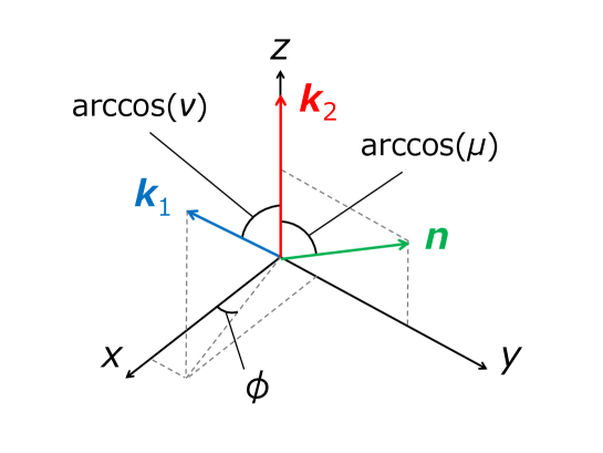
To evaluate the skewness parameters numerically, it is convenient to introduce the following coordinate system (see Fig. 2) as

$${\bm{n}}=(0,\sqrt{1-\mu^{2}},\mu)\,,$$ (107)

$${\bm{k}}_{1}=\frac{p}{R}(\sqrt{1-\nu^{2}}\cos\phi,\sqrt{1-\nu^{2}}\sin\phi,\nu)\,,$$ (108)

$${\bm{k}}_{2}=\frac{q}{R}(0,0,1)\,.$$ (109)

By adopting this coordinate system, the integration can reduce to

$$\int\frac{\mathrm{d}^{3}{\bm{k}}_{1}}{(2\pi)^{3}}\frac{\mathrm{d}^{3}{\bm{k}}_{2}}{(2\pi)^{3}}\to\frac{1}{32\pi^{5}R^{6}}\int_{0}^{\infty}p^{2}\mathrm{d}p\int_{0}^{\infty}q^{2}\mathrm{d}q\int_{-1}^{1}\mathrm{d}\mu\int_{-1}^{1}\mathrm{d}\nu\int_{0}^{2\pi}\mathrm{d}\phi\,,$$ (110)

and the skewness parameters can be simplified as

$$S_{\rm g,s}^{(a=0,1,2)}=\frac{b_{1}^{3}}{8\pi^{4}R^{2a+6}\sigma_{{\rm g}0}^{4-2a}\sigma_{{\rm g}1}^{2a}}\int_{0}^{\infty}\mathrm{d}p\int_{0}^{\infty}\mathrm{d}qe^{-(p^{2}+q^{2})}\widetilde{S}_{\rm s}^{(a=0,1,2)}(p,q)P_{\rm L}\left(\frac{p}{R}\right)P_{\rm L}\left(\frac{q}{R}\right)\,,$$ (111)

$$S_{\rm g,s}^{(3)}=\frac{b_{1}^{3}}{8\pi^{4}R^{8}\sigma_{{\rm g}0}^{2}\sigma_{{\rm g}\parallel}^{2}}\int_{0}^{\infty}\mathrm{d}p\int_{0}^{\infty}\mathrm{d}qe^{-(p^{2}+q^{2})}\widetilde{S}_{\rm s}^{(3)}(p,q)P_{\rm L}\left(\frac{p}{R}\right)P_{\rm L}\left(\frac{q}{R}\right)\,,$$ (112)

$$S_{\rm g,s}^{(4)}=\frac{b_{1}^{3}}{8\pi^{4}R^{10}\sigma_{{\rm g}\perp}^{2}\sigma_{{\rm g}\parallel}^{2}}\int_{0}^{\infty}\mathrm{d}p\int_{0}^{\infty}\mathrm{d}qe^{-(p^{2}+q^{2})}\widetilde{S}_{\rm s}^{(4)}(p,q)P_{\rm L}\left(\frac{p}{R}\right)P_{\rm L}\left(\frac{q}{R}\right)\,,$$ (113)

where $\widetilde{S}_{\rm g,s}^{(A)}(p,q)$ with $A=0,\cdots,4$ are kernel functions defined as

$$\widetilde{S}_{\rm g,s}^{(A)}(p,q)=\frac{6p^{2}q^{2}}{b_{1}^{3}}\int_{-1}^{1}\mathrm{d}\nu e^{-pq\nu}\int_{-1}^{1}\frac{\mathrm{d}\mu}{2}Z_{1}(\mu)\int_{0}^{2\pi}\frac{\mathrm{d}\phi}{2\pi}\,\widetilde{s}^{(A),{\rm sym}}(p,q,\nu,\mu_{1})Z_{1}(\mu_{1})Z_{2}(p,q,\mu,\nu,\mu_{1},\mu_{12})\,.$$ (114)

Here, $\widetilde{s}^{(0,1,2),{\rm sym}}$ in this coordinate system has the same form introduced in Eqs. (36)–(38), and $\widetilde{s}^{(3,4),{\rm sym}}$ is given by

$$\widetilde{s}^{(3),{\rm sym}}=\frac{1}{2}\Bigl{[}\left(p^{2}\mu_{1}^{2}+q^{2}\mu^{2}+pq\mu\mu_{1}\right)-\frac{1}{3}\left(p^{2}+q^{2}+pq\nu\right)\Bigr{]}\,,$$ (115)

$$\widetilde{s}^{(4),{\rm sym}}=\frac{3p^{2}q^{2}}{4}\Bigl{[}\left(\mu^{2}+\mu_{1}^{2}-2\mu\mu_{1}\nu\right)-\frac{2}{3}\left(1-\nu^{2}\right)\Bigr{]}\,.$$ (116)

In order to evaluate the skewness parameters Eqs. (111)–(113), we rewrite the first- and second-order kernels in redshift space, Eqs. (97) and (98), in terms of the coordinate system defined in Eqs. (107)–(109). With these notations, the first- and second-order kernels in redshift space can be given by

$$\frac{1}{b_{1}}Z_{1}(\mu)=1+\beta\mu^{2}\,,$$ (117)

$$\frac{2}{b_{1}}Z_{2}(p,q,\mu,\nu,\mu_{1},\mu_{12})=g_{0}\mathsf{P}_{0}+g_{1}\mathsf{P}_{1}+g_{2}\mathsf{P}_{2}+\beta\mu_{12}^{2}\Bigl{(}g_{3}\mathsf{P}_{3}+g_{4}\mathsf{P}_{4}\Bigr{)}+\mathsf{P}_{\ast}\,,$$ (118)

where $\mathsf{P}_{0,1,2}$ was already introduced in Eq. (41), and the remaining $\mathsf{P}_{3,4}$ and $\mathsf{P}_{\ast}$ are defined as

$$\mathsf{P}_{3}=\frac{1}{2}\left(\frac{p}{q}+\frac{q}{p}\right)P_{1}(\nu)+1\,,\ \ \mathsf{P}_{4}=P_{2}(\nu)-1\,,$$ (119)

$$\mathsf{P}_{\ast}=\beta\mu_{12}\sqrt{p^{2}+q^{2}+2pq\nu}\bigg{\{}\frac{\mu_{1}}{p}(1+\beta\mu^{2})+\frac{\mu}{q}(1+\beta\mu_{1}^{2})\biggr{\}}\,.$$ (120)

Here, $g_{0,1,2}$ has been defined in Eqs. (42)–(44) and we have introduced two new variables

$$g_{3}=\kappa_{\theta}\,,$$ (121)

$$g_{4}=\frac{16}{21}\lambda_{\theta}\,.$$ (122)

In the limit of the Einstein-de Sitter Universe without the nonlinear bias factor, $g_{0}=34/21$, $g_{1}=1$, $g_{2}=8/21$, $g_{3}=1$, and $g_{4}=16/21$.

III.3 Consistency relation in redshift space

Even when the redshift-space distortion effect is taken into account, $g_{I}$ ($I=0,\cdots,4$) appears in the skewness parameters linearly. Hence the redshift-space anisotropic skewness parameters can be algebraically rewritten as

$$S_{\rm g,s}^{(A)}=\sum_{I=0}^{4}\mathsf{M}_{\rm s}^{(A)}{}_{(I)}\,g_{I}+\mathsf{N}_{\rm s}^{(A)}\,,$$ (123)

where we have introduced the matrix $\mathsf{M}_{\rm s}$ which is defined as

$$\mathsf{M}_{\rm s}^{(A)}{}_{(I)}:=\frac{\partial S_{\rm g,s}^{(A)}}{\partial g_{I}}\,.$$ (124)

Unlike the real-space analysis, the above equation includes the term independent of $g_{I}$, $\mathsf{N}_{\rm s}$, which is directly related to the last term $P_{\ast}$ in Eq. (118). The explicit forms of the components $\mathsf{M}_{\rm s}$ and $\mathsf{N}_{\rm s}$ are shown in Appendix A.

Only when the determinant of $\mathsf{M}_{\rm s}$ is nonzero, Eq. (123) can be solved as

$$g_{I}=\sum_{A=0}^{4}[\mathsf{M}_{\rm s}^{-1}]^{(I)}{}_{(A)}\left(S_{\rm g,s}^{(A)}-\mathsf{N}_{\rm s}^{(A)}\right)\,.$$ (125)

As we mentioned in the previous section, the nontrivial signals of gravity theories appearing in the first and third equations would be hidden by the uncertainty of the nonlinear bias factors. Namely, the first and third equations would not be suitable for extracting the information of $g_{0}$ and $g_{2}$. On the other hand, as for the fourth and fifth terms corresponding to the new contributions from the mapping from real space to redshift space, Eqs. (121) and (122) imply that there appear no bias contributions. Hence, the redshift-space anisotropic contributions to the skewness parameters can be used to extract the information from gravity theory without suffering from the uncertainty of the nonlinear galaxy bias. We finally have the three meaningful consistency relations in redshift space:

$$g_{1}=\kappa=\sum_{A=0}^{4}[\mathsf{M}_{\rm s}^{-1}]^{(1)}{}_{(A)}\left(S_{\rm g,s}^{(A)}-\mathsf{N}_{\rm s}^{(A)}\right)\,,$$ (126)

$$g_{3}=\kappa_{\theta}=\sum_{A=0}^{4}[\mathsf{M}_{\rm s}^{-1}]^{(3)}{}_{(A)}\left(S_{\rm g,s}^{(A)}-\mathsf{N}_{\rm s}^{(A)}\right)\,,$$ (127)

$$g_{4}=\frac{16}{21}\lambda_{\theta}=\sum_{A=0}^{4}[\mathsf{M}_{\rm s}^{-1}]^{(4)}{}_{(A)}\left(S_{\rm g,s}^{(A)}-\mathsf{N}_{\rm s}^{(A)}\right)\,.$$ (128)

These are also the main results of this paper. When gravity is described by the Horndeski scalar-tensor theory Horndeski:1974wa ; Deffayet:2011gz ; Kobayashi:2011nu including general relativity, we have $\kappa=\kappa_{\theta}=1$, while $\lambda_{\theta}$ generally deviates from unity Takushima:2013foa ; Yamauchi:2017ibz . Therefore, Eqs. (126) and (127) provide the consistency relations between the anisotropic skewness parameters, and we can extract the information on the modification of gravity theory from Eq. (128). In the case of the extension of the Horndeski theory such as the DHOST theories Langlois:2015cwa ; Crisostomi:2016czh ; Achour:2016rkg ; BenAchour:2016fzp , $\kappa$ and $\kappa_{\theta}$ also deviate from unity Hirano:2018uar ; Crisostomi:2019vhj ; Lewandowski:2019txi ; Hirano:2020dom ; Yamauchi:2021nxw . Therefore, if the combinations of the skewness parameters given by the RHS of Eqs. (126) and (127) depart from unity, it would be the signals of the beyond-Honrdeski class of gravity theories.

Although the consistency relation for an arbitrary value of $\beta$ can be obtained by solving the formulae (126)–(128) numerically, in order to see the qualitative behavior of these consistency relations, we consider the small-$\beta$ approximation, which corresponds to the case of the large linear galaxy bias, such as in the case of very massive haloes. It is expected that the asymptotes of the equations for the redshift-space skewness parameters in the limit of $\beta\to 0$ should reproduce the real-space ones. The coefficient matrix $\mathsf{M}_{\rm s}$, the vector $\mathsf{N}_{\rm s}^{(A)}$, and the redshift-space skewness parameters $S_{\rm s}^{(A)}$ can be expanded in terms of $\beta$ as

$$\mathsf{M}_{\rm s}=\left(\begin{array}[]{c|c}\mathsf{M}_{\rm r}&0_{2\times 3}\\ \hline\cr 0_{3\times 2}&0_{2\times 2}\\ \end{array}\right)+\left(\begin{array}[]{c|c}\mathsf{A}&\mathsf{B}\\ \hline\cr\mathsf{C}&\mathsf{D}\\ \end{array}\right)\beta+{\cal O}(\beta^{2})\,,$$ (133)

$$\mathsf{N}_{\rm s}^{(A)}=\delta\mathsf{N}_{\rm s}^{(A)}\,\beta+{\cal O}(\beta^{2})\,,$$ (134)

$$S_{\rm g,s}^{(A)}=\left(\begin{array}[]{c}\overline{S}_{\rm g,s}^{(a)}\\ \hline\cr 0_{1\times 2}\\ \end{array}\right)+\delta S_{\rm g,s}^{(A)}\,\beta+{\cal O}(\beta^{2})\,,$$ (137)

with $0_{m,n}$ denoting the $m\times n$ zero matrix. The inverse of the matrix $\mathsf{M}_{\rm s}$ is approximately given as

$$\mathsf{M}_{\rm s}^{-1}=\left(\begin{array}[]{c|c}0_{3\times 3}&0_{3\times 2}\\ \hline\cr 0_{2\times 3}&\mathsf{D}^{-1}\\ \end{array}\right)\frac{1}{\beta}+\left(\begin{array}[]{c|c}\mathsf{M}_{\rm r}^{-1}&-\mathsf{M}_{\rm r}^{-1}\mathsf{B}\mathsf{D}^{-1}\\ \hline\cr-\mathsf{D}^{-1}\mathsf{C}\mathsf{M}_{\rm r}^{-1}&\ast\\ \end{array}\right)+{\cal O}(\beta)\,,$$ (142)

where the symbol $\ast$ denotes the arbitrary matrix components. This is because this term gives only the ${\cal O}(\beta^{2})$ subleading correction in the skewness consistency conditions. Hence, in our situation, considering the ${\cal O}(\beta)$ term in $\mathsf{M}_{\rm s}^{-1}$ is enough to provide the leading consistency relation. The leading order expression of (125) for the first three $g_{I=0,1,2}$ appears at order ${\cal O}(\beta^{0})$:

$$g_{I}=\sum_{A=0}^{2}[\mathsf{M}_{\rm r}^{-1}]^{(I)}{}_{(A)}S_{\rm g,s}^{(A)}+{\cal O}(\beta)\ \ \ \text{for}\ I=0,1,2\,.$$ (143)

It is obvious that the above equation is the same as the consistency relation in real space, Eq. (50), except for the ${\cal O}(\beta)$ correction, as expected. Hence, the nontrivial consistency relation in redshift space can be obtained from the remaining parts. As for the remaining two equations for $I=3,4$, the ${\cal O}(\beta^{0})$ equation vanishes and the next-leading order equations at ${\cal O}(\beta)$ are given as

$$\beta g_{I}=\beta\biggl{[}-\sum_{a=0}^{2}[\mathsf{D}^{-1}\mathsf{C}\mathsf{M}_{\rm r}^{-1}]^{(I)}{}_{(a)}\overline{S}_{\rm g,s}^{(a)}+\sum_{A=3}^{4}[\mathsf{D}^{-1}]^{(I)}{}_{(A)}\left(\delta S_{\rm g,s}^{(A)}-\delta\mathsf{N}_{\rm s}^{(A)}\right)\biggr{]}+{\cal O}(\beta^{2})\ \ \ \text{for}\ I=3,4\,.$$ (144)

We note that one cannot use the above equation in the limit of $\beta\to 0$ since the inverse of the matrix $\mathsf{M}_{\rm s}$, Eq. (142), in such a limit becomes singular.

Finally, let us evaluate $\mathsf{M}_{\rm s}$ and $\mathsf{N}_{\rm s}$ up to ${\cal O}(\beta)$ with $R=10\,h^{-1}\,{\rm Mpc}$:

$$\mathsf{M}_{\rm s}=\frac{1}{b_{1}}\left(\begin{array}[]{ccccc}3.4930&-2.1752&0.21206&0&0\\ 3.4049&-1.9486&0.17288&0&0\\ 4.2484&-3.0888&-0.34998&0&0\\ 0&0&0&0&0\\ 0&0&0&0&0\\ \end{array}\right)$$ (150)

$$\qquad\qquad+\frac{1}{b_{1}}\left(\begin{array}[]{ccccc}2.3287&-1.4501&0.14137&0.80182&-1.0937\\ 2.2699&-1.2991&0.11526&0.81021&-1.0773\\ 2.8232&-2.0585&-0.23332&0.90152&-1.5328\\ 0.86098&-0.51106&0.22433&0.50322&-0.57462\\ 0.84969&-0.61755&-0.07000&0.27046&-0.45984\\ \end{array}\right)\beta+{\cal O}(\beta^{2})\,,$$ (156)

$$\mathsf{N}_{\rm s}^{(A)}=\frac{1}{b_{1}}\left(\begin{array}[]{c}1.6036\\ 1.6204\\ 1.8030\\ 0.81884\\ 0.54091\\ \end{array}\right)\beta+{\cal O}(\beta^{2})\,,$$ (162)

which immediately leads the leading-order consistency relations (143) and (144) as

$$\frac{1}{b_{1}}\kappa=-4.621\overline{S}_{\rm g,s}^{(0)}+5.094\overline{S}_{\rm g,s}^{(1)}-0.283\overline{S}_{\rm g,s}^{(2)}+{\cal O}(\beta)\,,$$ (163)

$$\beta\frac{1}{b_{1}}\kappa_{\theta}=\beta\biggl{[}-6.373\overline{S}_{\rm g,s}^{(0)}+3.085\overline{S}_{\rm g,s}^{(1)}+3.054\overline{S}_{\rm g,s}^{(2)}+6.051\left(\delta S_{\rm g,s}^{(3)}-\frac{0.819}{b_{1}}\right)-7.562\left(\delta S_{\rm g,s}^{(4)}-\frac{0.541}{b_{1}}\right)\biggr{]}+{\cal O}(\beta^{2})\,,$$ (164)

$$\beta\frac{1}{b_{1}}\frac{16}{21}\lambda_{\theta}=\beta\biggl{[}-3.748\overline{S}_{\rm g,s}^{(0)}+1.814\overline{S}_{\rm g,s}^{(1)}+2.231\overline{S}_{\rm g,s}^{(2)}+3.559\left(\delta S_{\rm g,s}^{(3)}-\frac{0.819}{b_{1}}\right)-6.622\left(\delta S_{\rm g,s}^{(4)}-\frac{0.541}{b_{1}}\right)\biggr{]}+{\cal O}(\beta^{2})\,.$$ (165)

The expression Eqs. (163)–(165) are valid only when $\beta$ is nonvanishing but very small. In the case of the realistic situation with the non-negligible value of $\beta$, the numerical evaluation of all the components of $\mathsf{M}_{\rm s}$ and $\mathsf{N}_{\rm s}$ is needed through Eqs. (126)–(128). An interesting observation is that the linear combination of the two equations (164) and (165) gives the nontrivial equation as

$$\beta\left(\frac{1}{b_{1}}\kappa_{\theta}-1.700\frac{1}{b_{1}}\frac{16}{21}\lambda_{\theta}\right)=0.739\beta\left(\overline{S}_{\rm g,s}^{(2)}-5\,\delta S_{\rm g,s}^{(4)}\right)+{\cal O}(\beta^{2})\,,$$ (166)

which implies that we can extract the information of the specific combination of $\kappa_{\theta}$ and $\lambda_{\theta}$ from $S_{\rm g,s}^{(2)}$ and $\delta S_{\rm g,s}^{(4)}$ alone. Although the detailed structure depends on the definition of the skewness parameters, this type of relationship between $\kappa_{\theta}$ and $\lambda_{\theta}$ can be numerically confirmed for any value of $R$. It would be interesting to evaluate the higher-order corrections for this type of relation.

IV Summary

In this paper, we have investigated the skewness as a possible probe to test the theory of gravity such as the Horndeski scalar-tensor theory and the degenerate higher-order scalar-tensor (DHOST) theory. We have developed the formula of the skewness for the galaxy number density fluctuations as realistic observables and have considered how the effect of the quasi-nonlinear growth of structure appears in the skewness parameters.

We have shown that the three time-dependent parameters including the coefficients of the kernels of the second-order density contrast can be rewritten in terms of the linear combination of the three skewness parameters in the real space. In two of the three equations, the signature of the modified gravity represented by the second-order kernels is hidden by the uncertainty in the nonlinear galaxy bias functions, but the remaining one can be used to extract the information of the gravity theory, in particular the DHOST theory, without suffering from the nonlinear bias [see Eq. (51)]. Even when the gravity is described by general relativity, the equation can be treated as the consistency relation among the three skewness parameters, which can be used as a test of gravity theory.

We then extended the analysis from the real space to the redshift space and properly identified the five independent redshift-space skewness parameters to characterize the anisotropy due to the redshift-space distortions. We found that three of these are the same as the real-space skewness parameters, while the two new type skewness parameters are needed [Eqs. (85) and (86)]. We have developed the analysis tool for the redshift-space skewness parameters and have shown the similar consistency relations to the real-space one. Unlike the real space, we found three nontrivial consistency relations, two of which are related to the second-order kernels of the peculiar velocity field [Eqs. (126)–(128)]. Using the resultant expressions, one can distinguish general relativity and the Horndeski scalar-tensor theory.

In this paper, we have only shown the presence of the consistency relations for the skewness parameters, but we have not addressed the forecast for current and future large-scale observations. Moreover, we have focused only on the specific type of second-order kernel functions. In the case of the Horndeski and DHOST theories with the quasi-static approximation, these expressions can be shown to be valid Hirano:2020dom . However, if the gravity theory is described by other types such as vector-tensor and bi-gravity theories, or if the quasi-static approximation is partially broken, there may appear correction terms in the kernel functions. In addition, in our formulation, the dependence on the linear galaxy bias function remains intact. Since the bias functions in a specific type of modified gravity theory may have the scale-dependence, evaluating the linear galaxy bias function under various gravity theories would be important for the error estimation. Hence, investigating how the gravity theory is severely constrained by using the consistency relation for current and future large-scale structure is interesting, but it is left for a future issue.

Appendix A Reduced expression

In this section, we show the explicit forms of the kernels of the skewness parameters by using the formula Eq. (114). For convenience, let us introduce the matrix and the vector defined as

$$\widetilde{\mathsf{M}}_{\rm s}{}^{(A)}{}_{(I)}(p,q):=\frac{6p^{2}q^{2}}{b_{1}^{3}}\int_{-1}^{1}\mathrm{d}\nu e^{-pq\nu}\int_{-1}^{1}\frac{\mathrm{d}\mu}{2}Z_{1}(\mu)\int_{0}^{2\pi}\frac{\mathrm{d}\phi}{2\pi}\,s^{(A),{\rm sym}}(p,q,\nu,\mu_{1})Z_{1}(\mu_{1})\frac{\partial Z_{2}(p,q,\mu,\nu,\mu_{1},\mu_{12})}{\partial g_{I}}\,,$$ (167)

$$\widetilde{\mathsf{N}}_{\rm s}^{(A)}(p,q):=\frac{6p^{2}q^{2}}{b_{1}^{3}}\int_{-1}^{1}\mathrm{d}\nu e^{-pq\nu}\int_{-1}^{1}\frac{\mathrm{d}\mu}{2}Z_{1}(\mu)\int_{0}^{2\pi}\frac{\mathrm{d}\phi}{2\pi}\,s^{(A),{\rm sym}}(p,q,\nu,\mu_{1})Z_{1}(\mu_{1})\frac{b_{1}}{2}\mathsf{P}_{\ast}(p,q,\mu,\nu,\mu_{1},\mu_{12})\,.$$ (168)

As a demonstration, let us consider the specific matrix components $\widetilde{\mathsf{M}}_{\rm s}^{(A=0,1,2)}{}_{(I=0,1,2)}$. The integration of $\phi$ and $\mu$ can be done analytically to obtain

$$\widetilde{\mathsf{M}}_{\rm s}^{(A=0,1,2)}{}_{(I=0,1,2)}= \,3p^{2}q^{2}\int_{-1}^{1}\mathrm{d}\nu s^{(A=0,1,2),{\rm sym}}(p,q,\nu)\mathsf{P}_{I=0,1,2}(p,q,\nu)e^{-pq\nu}\biggl{[}\left(1+\frac{1}{3}\beta\right)^{2}+\frac{4}{45}\beta^{2}P_{2}(\nu)\biggr{]}\,.$$ (169)

One can easily find from the above expression that the leading order terms at order ${\cal O}(\beta^{0})$ coincide with the real-space parts $\widetilde{\mathsf{M}}_{\rm r}^{(a)}{}_{(i)}:=\partial\widetilde{S}_{\rm r}^{(a)}/\partial g_{i}$ derived from Eqs. (45)–(47), and the correction terms appear as those with $\beta$ up to ${\cal O}(\beta^{2})$. The explicit form of the kernels after the integration of $\nu$ yields

$$\widetilde{\mathsf{M}}_{\rm s}^{(0)}{}_{(0)}=\left(1+\frac{1}{3}\beta\right)^{2}\widetilde{\mathsf{M}}_{\rm r}^{(0)}{}_{(0)}+\frac{8}{15}\beta^{2}\biggl{[}-3\left(\cosh(pq)-\frac{\sinh(pq)}{pq}\right)+pq\sinh(pq)\biggr{]}\,,$$ (170)

$$\widetilde{\mathsf{M}}_{\rm s}^{(0)}{}_{(1)}=\left(1+\frac{1}{3}\beta\right)^{2}\widetilde{\mathsf{M}}_{\rm r}^{(0)}{}_{(1)}+\frac{8}{15pq}\left(\frac{p}{q}+\frac{q}{p}\right)\beta^{2}\biggl{[}-\left(9+p^{2}q^{2}\right)\left(\cosh(pq)-\frac{\sinh(pq)}{pq}\right)+3pq\sinh(pq)\biggr{]}\,,$$ (171)

$$\widetilde{\mathsf{M}}_{\rm s}^{(0)}{}_{(2)}=\left(1+\frac{1}{3}\beta\right)^{2}\widetilde{\mathsf{M}}_{\rm r}^{(0)}{}_{(2)}+\frac{8}{15p^{2}q^{2}}\beta^{2}\biggl{[}-6\left(9+p^{2}q^{2}\right)\left(\cosh(pq)-\frac{\sinh(pq)}{pq}\right)+\left(18+p^{2}q^{2}\right)pq\sinh(pq)\biggr{]}\,,$$ (172)

for $A=0$,

$$\widetilde{\mathsf{M}}_{\rm s}^{(1)}{}_{(0)}=\left(1+\frac{1}{3}\beta\right)^{2}\widetilde{\mathsf{M}}_{\rm r}^{(1)}{}_{(0)}+\frac{4}{15}\beta^{2}\biggl{[}-(3+p^{2})(3+q^{2})\left(\cosh(pq)-\frac{\sinh(pq)}{pq}\right)+\left(3+p^{2}+q^{2}\right)pq\sinh(pq)\biggr{]}\,,$$ (173)

$$\widetilde{\mathsf{M}}_{\rm s}^{(1)}{}_{(1)}=\left(1+\frac{1}{3}\beta\right)^{2}\widetilde{\mathsf{M}}_{\rm r}^{(1)}{}_{(1)}$$

$$\qquad\qquad\qquad+\frac{4}{15pq}\left(\frac{p}{q}+\frac{q}{p}\right)\beta^{2}\biggl{[}-\Bigl{\{}p^{2}q^{2}(2+p^{2}+q^{2})+3(3+p^{2})(3+q^{2})+9\Bigr{\}}\left(\cosh(pq)-\frac{\sinh(pq)}{pq}\right)$$

$$\qquad\qquad\qquad+\Bigl{\{}(3+p^{2})(3+q^{2})+3\Bigr{\}}pq\sinh(pq)\biggr{]}\,,$$ (174)

$$\widetilde{\mathsf{M}}_{\rm s}^{(1)}{}_{(2)}=\left(1+\frac{1}{3}\beta\right)^{2}\widetilde{\mathsf{M}}_{\rm r}^{(1)}{}_{(2)}+\frac{4}{15p^{2}q^{2}}\beta^{2}\biggl{[}-\Big{\{}54(5+p^{2}+q^{2})+p^{2}q^{2}(6+p^{2})(6+q^{2})\Bigr{\}}\left(\cosh(pq)-\frac{\sinh(pq)}{pq}\right)$$

$$\qquad\qquad\qquad+\Bigl{\{}18(5+p^{2}+q^{2})+p^{2}q^{2}(6+p^{2}+q^{2})\Bigr{\}}pq\sinh(pq)\biggr{]}\,,$$ (175)

for $A=1$, and

$$\widetilde{\mathsf{M}}_{\rm s}^{(2)}{}_{(0)}=\left(1+\frac{1}{3}\beta\right)^{2}\widetilde{\mathsf{M}}_{\rm r}^{(2)}{}_{(0)}+\frac{8}{5}\beta^{2}\biggl{[}\left(18+p^{2}q^{2}\right)\left(\cosh(pq)-\frac{\sinh(pq)}{pq}\right)-6pq\sinh(pq)\biggr{]}\,,$$ (176)

$$\widetilde{\mathsf{M}}_{\rm s}^{(2)}{}_{(1)}=\left(1+\frac{1}{3}\beta\right)^{2}\widetilde{\mathsf{M}}_{\rm r}^{(2)}{}_{(1)}+\frac{8}{5pq}\left(\frac{p}{q}+\frac{q}{p}\right)\beta^{2}\biggl{[}9\left(10+p^{2}q^{2}\right)\left(\cosh(pq)-\frac{\sinh(pq)}{pq}\right)-\left(30+p^{2}q^{2}\right)pq\sinh(pq)\biggr{]}\,,$$ (177)

$$\widetilde{\mathsf{M}}_{\rm s}^{(2)}{}_{(2)}=\left(1+\frac{1}{3}\beta\right)^{2}\widetilde{\mathsf{M}}_{\rm r}^{(2)}{}_{(2)}$$

$$\qquad\qquad\qquad+\frac{8}{5p^{2}q^{2}}\beta^{2}\biggl{[}\left(810+90p^{2}q^{2}+p^{4}q^{4}\right)\left(\cosh(pq)-\frac{\sinh(pq)}{pq}\right)-6\left(45+2p^{2}q^{2}\right)pq\sinh(pq)\biggr{]}\,,$$ (178)

for $A=2$.

Hereafter, we give up showing all the results since the resultant expressions are very long. Instead, we will show the kernels before the $\nu$ integration. One can easily obtain the result after the $\nu$ integration analytically. In the case of $A=0,1,2$ with $I=3,4$, after the integration of $\phi$ and $\mu$, we have

$$\widetilde{\mathsf{M}}_{\rm s}^{(A=0,1,2)}{}_{(I=3,4)}=3p^{2}q^{2}\beta\int_{-1}^{1}\mathrm{d}\nu s^{(0,1,2),{\rm sym}}(p,q,\nu)\mathsf{P}_{3,4}(p,q,\nu)e^{-pq\nu}$$

$$\qquad\times\frac{1}{105}\biggl{[}\Bigl{\{}7(5+4\beta+2\beta\nu^{2})+3\beta^{2}(1+4\nu^{2})\Bigr{\}}+\frac{4\beta(7+3\beta)pq\nu(1-\nu^{2})}{p^{2}+q^{2}+2pq\nu}\biggr{]}\,.$$ (179)

Let us move on to the case with $A=3,4$. In this case, the integration of $\phi$ and $\mu$ leads to

$$\widetilde{\mathsf{M}}_{\rm s}^{(3)}{}_{(I)}=\frac{p^{2}q^{2}}{70}\int_{-1}^{1}\mathrm{d}\nu\mathsf{P}_{I}(p,q,\nu)e^{-pq\nu}$$

$$\qquad\times\biggl{[}\left(p^{2}+q^{2}+pq\nu\right)\Bigl{\{}35+14\beta(2+\nu^{2})+3\beta^{2}(1+4\nu^{2})\Bigr{\}}+2\beta(7+3\beta)pq\nu\left(1-\nu^{2}\right)\biggr{]}-\frac{1}{3}\widetilde{\mathsf{M}}_{\rm s}^{(1)}{}_{(I)}\,,$$ (180)

$$\widetilde{\mathsf{M}}_{\rm s}^{(4)}{}_{(I)}=\frac{3p^{4}q^{4}}{70}\int_{-1}^{1}\mathrm{d}\nu\mathsf{P}_{I}(p,q,\nu)e^{-pq\nu}\Bigl{\{}35+28\beta+3\beta^{2}(1+2\nu^{2})\Bigr{\}}\left(1-\nu^{2}\right)-\frac{1}{3}\widetilde{\mathsf{M}}_{\rm s}^{(2)}{}_{(I)}\,,$$ (181)

for $I=0,1,2$, and

$$\widetilde{\mathsf{M}}_{\rm s}^{(3)}{}_{(I)}=\frac{p^{2}q^{2}}{210}\beta\int_{-1}^{1}\mathrm{d}\nu\mathsf{P}_{3,4}(p,q,\nu)e^{-pq\nu}\biggl{[}3pq\nu\Bigl{\{}63+18\beta(4+\nu^{2})+5\beta^{2}(3+4\nu^{2})\Bigr{\}}$$

$$\qquad\qquad+\frac{1}{p^{2}+q^{2}+2pq\nu}\bigg{\{}21\Bigl{[}3(p^{4}+q^{4})+2p^{2}q^{2}(2-5\nu^{2})\Bigr{]}+18\Bigl{[}(p^{4}+q^{4})(3+2\nu^{2})-2p^{2}q^{2}(-2+4\nu^{2}+3\nu^{4})\Bigr{]}\beta$$

$$\qquad\qquad\qquad\qquad\qquad+\Bigl{[}5(p^{4}+q^{4})(1+6\nu^{2})+2p^{2}q^{2}(6+3\nu^{2}-44\nu^{4})\Bigr{]}\beta^{2}\biggr{\}}\biggr{]}-\frac{1}{3}\widetilde{\mathsf{M}}_{\rm s}^{(1)}{}_{(I)}\,,$$ (182)

$$\widetilde{\mathsf{M}}_{\rm s}^{(4)}{}_{(I)}=\frac{p^{4}q^{4}}{35}\beta\int_{-1}^{1}\mathrm{d}\nu\mathsf{P}_{3,4}(p,q,\nu)e^{-pq\nu}\biggl{[}21+9(2+\nu^{2})\beta+2(1+4\nu^{2})\beta^{2}+\frac{2pq\nu\beta(9+4\beta)(1-\nu^{2})}{p^{2}+q^{2}+2pq\nu}\biggr{]}(1-\nu^{2})$$

$$\qquad\qquad-\frac{1}{3}\widetilde{\mathsf{M}}_{\rm s}^{(2)}{}_{(I)}\,,$$ (183)

for $I=3,4$. In the limit of $\beta\to 0$, one explicitly shows that $\widetilde{\mathsf{M}}_{\rm s}^{(3,4)}{}_{(I)}$ becomes zero since we imposed the anisotropic part of the skewness parameters in the isotropic limit ($\beta\to 0$) reduces to zero. We note that the ${\cal O}(\beta)$ correction term of the specific component, $\widetilde{\mathsf{M}}_{\rm s}^{(4)}{}_{(0,1,2)}$, can be rewritten in terms of the ${\cal O}(\beta^{0})$ part of $\widetilde{\mathsf{M}}_{\rm s}^{(2)}{}_{(0,1,2)}$.

Finally, we show the expressions for $\widetilde{\mathsf{N}}_{\rm s}$:

$$\widetilde{\mathsf{N}}_{\rm s}^{(A=0,1,2)}=3p^{2}q^{2}\beta\int_{-1}^{1}\mathrm{d}\nu s^{(0,1,2),{\rm sym}}(p,q,\nu)e^{-pq\nu}\Bigg{[}\frac{1}{3}\biggl{\{}2+\nu\left(\frac{p}{q}+\frac{q}{p}\right)\biggr{\}}+\frac{1}{15}\biggl{\{}10+8\nu^{2}+9\nu\left(\frac{p}{q}+\frac{q}{p}\right)\biggr{\}}\beta$$

$$\qquad+\frac{1}{35}\biggl{\{}6(1+4\nu^{2})+\left(11+4\nu^{2}\right)\nu\left(\frac{p}{q}+\frac{q}{p}\right)\biggr{\}}\beta^{2}+\frac{1}{315}\biggl{\{}6+16\nu^{2}(3+\nu^{2})+5\nu(3+4\nu^{2})\left(\frac{p}{q}+\frac{q}{p}\right)\biggr{\}}\beta^{3}\Biggr{]}\,,$$ (184)

for $A=0,1,2$, and

$$\widetilde{\mathsf{N}}_{\rm s}^{(3)}=\frac{3pq}{2}\beta\int_{-1}^{1}\mathrm{d}\nu e^{-pq\nu}\Biggl{[}\frac{1}{15}\Bigl{\{}pq(p^{2}+q^{2})(5+4\nu^{2})+3(p^{4}+4p^{2}q^{2}+q^{4})\nu\Bigr{\}}$$

$$\qquad\qquad+\frac{1}{35}\Bigl{\{}\nu(p^{4}+q^{4})(13+2\nu^{2})+4p^{2}q^{2}\nu(11+4\nu^{2})+pq(p^{2}+q^{2})(13+32\nu^{2})\Bigr{\}}\beta$$

$$\qquad\qquad+\frac{1}{63}\Bigl{\{}12p^{2}q^{2}\nu(3+4\nu^{2})+(p^{4}+q^{4})\nu(13+8\nu^{2})+pq(p^{2}+q^{2})(7+48\nu^{2}+8\nu^{4})\Bigr{\}}\beta^{2}$$

$$\qquad\qquad+\frac{1}{693}\Bigl{\{}21(p^{4}+q^{4})\nu(1+2\nu^{2})+9pq(p^{2}+q^{2})(1+12\nu^{2}+8\nu^{4})+4p^{2}q^{2}\nu(15+40\nu^{2}+8\nu^{4})\Bigr{\}}\beta^{3}\Biggr{]}$$

$$\qquad\qquad-\frac{1}{3}\widetilde{\mathsf{N}}_{\rm s}^{(1)}\,,$$ (185)

$$\widetilde{\mathsf{N}}_{\rm s}^{(4)}=-\frac{9p^{3}q^{3}}{4}\beta\int_{-1}^{1}\mathrm{d}\nu e^{-pq\nu}\Biggl{[}\frac{4}{15}\Big{\{}2pq+(p^{2}+q^{2})\nu\Bigr{\}}+\frac{2}{35}\Bigl{\{}2pq(5+4\nu^{2})+9(p^{2}+q^{2})\nu\Bigr{\}}\beta$$

$$\qquad\qquad+\frac{8}{315}\Bigl{\{}6pq(1+4\nu^{2})+(p^{2}+q^{2})(11+4\nu^{2})\nu\Bigr{\}}\beta^{2}$$

$$\qquad\qquad+\frac{2}{693}\Bigl{\{}5(p^{2}+q^{2})\nu(3+4\nu^{2})+2pq\left(3+24\nu^{2}+8\nu^{4}\right)\Bigr{\}}\beta^{3}\Biggr{]}(1-\nu^{2})-\frac{1}{3}\widetilde{\mathsf{N}}_{\rm s}^{(2)}\,,$$ (186)

for $A=3,4$.

References

- (1) P. J. E. Peebles, The Large-scale Structure of the Universe (Princeton, Princeton University Press, 1980).
- (2) F. Bernardeau, S. Colombi, E. Gaztanaga and R. Scoccimarro, Phys. Rept. 367 (2002), 1-248 doi:10.1016/S0370-1573(02)00135-7 [arXiv:astro-ph/0112551 [astro-ph]].
- (3) T. Matsubara, Astrophys. J. Lett. 434 (1994), L43 doi:10.1086/187570 [arXiv:astro-ph/9405037 [astro-ph]].
- (4) T. Matsubara, Astrophys. J. 584 (2003), 1-33 doi:10.1086/345521
- (5) Y. Takushima, A. Terukina and K. Yamamoto, Phys. Rev. D 89 (2014) no.10, 104007 doi:10.1103/PhysRevD.89.104007 [arXiv:1311.0281 [astro-ph.CO]].
- (6) Y. Takushima, A. Terukina and K. Yamamoto, Phys. Rev. D 92 (2015) no.10, 104033 doi:10.1103/PhysRevD.92.104033 [arXiv:1502.03935 [gr-qc]].
- (7) D. Yamauchi, S. Yokoyama and H. Tashiro, Phys. Rev. D 96 (2017) no.12, 123516 doi:10.1103/PhysRevD.96.123516 [arXiv:1709.03243 [astro-ph.CO]].
- (8) S. Hirano, T. Kobayashi, H. Tashiro and S. Yokoyama, Phys. Rev. D 97 (2018) no.10, 103517 doi:10.1103/PhysRevD.97.103517 [arXiv:1801.07885 [astro-ph.CO]].
- (9) M. Crisostomi, M. Lewandowski and F. Vernizzi, Phys. Rev. D 101 (2020) no.12, 123501 doi:10.1103/PhysRevD.101.123501 [arXiv:1909.07366 [astro-ph.CO]].
- (10) M. Lewandowski, JCAP 08 (2020), 044 doi:10.1088/1475-7516/2020/08/044 [arXiv:1912.12292 [astro-ph.CO]].
- (11) S. Hirano, T. Kobayashi, D. Yamauchi and S. Yokoyama, Phys. Rev. D 102 (2020) no.10, 103505 doi:10.1103/PhysRevD.102.103505 [arXiv:2008.02798 [gr-qc]].
- (12) D. Yamauchi and N. S. Sugiyama, Phys. Rev. D 105 (2022) no.6, 063515 doi:10.1103/PhysRevD.105.063515 [arXiv:2108.02382 [astro-ph.CO]].
- (13) T. Namikawa, F. R. Bouchet and A. Taruya, Phys. Rev. D 98 (2018) no.4, 043530 doi:10.1103/PhysRevD.98.043530 [arXiv:1805.10567 [astro-ph.CO]].
- (14) T. Matsubara, C. Hikage and S. Kuriki, Phys. Rev. D 105 (2022) no.2, 023527 doi:10.1103/PhysRevD.105.023527 [arXiv:2012.00203 [astro-ph.CO]].
- (15) V. Desjacques, D. Jeong and F. Schmidt, Phys. Rept. 733 (2018), 1-193 doi:10.1016/j.physrep.2017.12.002 [arXiv:1611.09787 [astro-ph.CO]].
- (16) F. R. Bouchet, S. Colombi, E. Hivon and R. Juszkiewicz, Astron. Astrophys. 296 (1995), 575 [arXiv:astro-ph/9406013 [astro-ph]].
- (17) G. W. Horndeski, Int. J. Theor. Phys. 10 (1974), 363-384 doi:10.1007/BF01807638
- (18) C. Deffayet, X. Gao, D. A. Steer and G. Zahariade, Phys. Rev. D 84 (2011), 064039 doi:10.1103/PhysRevD.84.064039 [arXiv:1103.3260 [hep-th]].
- (19) T. Kobayashi, M. Yamaguchi and J. Yokoyama, Prog. Theor. Phys. 126 (2011), 511-529 doi:10.1143/PTP.126.511 [arXiv:1105.5723 [hep-th]].
- (20) D. Langlois and K. Noui, JCAP 02 (2016), 034 doi:10.1088/1475-7516/2016/02/034 [arXiv:1510.06930 [gr-qc]].
- (21) M. Crisostomi, K. Koyama and G. Tasinato, JCAP 04 (2016), 044 doi:10.1088/1475-7516/2016/04/044 [arXiv:1602.03119 [hep-th]].
- (22) J. Ben Achour, D. Langlois and K. Noui, Phys. Rev. D 93 (2016) no.12, 124005 doi:10.1103/PhysRevD.93.124005 [arXiv:1602.08398 [gr-qc]].
- (23) J. Ben Achour, M. Crisostomi, K. Koyama, D. Langlois, K. Noui and G. Tasinato, JHEP 12 (2016), 100 doi:10.1007/JHEP12(2016)100 [arXiv:1608.08135 [hep-th]].
- (24) D. Langlois, R. Saito, D. Yamauchi and K. Noui, Phys. Rev. D 97 (2018) no.6, 061501 doi:10.1103/PhysRevD.97.061501 [arXiv:1711.07403 [gr-qc]].
- (25) D. Langlois, Int. J. Mod. Phys. D 28 (2019) no.05, 1942006 doi:10.1142/S0218271819420069 [arXiv:1811.06271 [gr-qc]].
- (26) T. Kobayashi, Rept. Prog. Phys. 82 (2019) no.8, 086901 doi:10.1088/1361-6633/ab2429 [arXiv:1901.07183 [gr-qc]].
- (27) D. J. Eisenstein and W. Hu, Astrophys. J. 496 (1998), 605 doi:10.1086/305424 [arXiv:astro-ph/9709112 [astro-ph]].
- (28) S. Codis, C. Pichon, D. Pogosyan, F. Bernardeau and T. Matsubara, Mon. Not. Roy. Astron. Soc. 435 (2013), 531-564 doi:10.1093/mnras/stt1316 [arXiv:1305.7402 [astro-ph.CO]].
- (29) R. Scoccimarro, H. M. P. Couchman and J. A. Frieman, Astrophys. J. 517 (1999), 531-540 doi:10.1086/307220 [arXiv:astro-ph/9808305 [astro-ph]].