Limitations of Quantum Measurements and Operations of Scattering Type under the Energy Conservation Law

Abstract

It is important to improve the accuracy of quantum measurements and operations both in engineering and fundamental physics. It is known, however, that the achievable accuracy of measurements and unitary operations are generally limited by conservation laws according to the Wigner–Araki–Yanase theorem (WAY theorem) and its generalizations. Although many researches have extended the WAY theorem quantitatively, most of them, as well as the original WAY theorem, concern only additive conservation laws like the angular momentum conservation law. In this paper, we explore the limitation incurred by the energy conservation law, which is universal but is one of the non-additive conservation laws. We present a lower bound for the error of a quantum measurement using a scattering process satisfying the energy conservation law. We obtain conditions that a control system Hamiltonian must fulfill in order to implement a controlled unitary gate with zero error when a scattering process is considered. We also show the quantitative relationship between the upper bound of the gate fidelity of a controlled unitary gate and the energy fluctuation of systems when a target system and a control system are both one qubit.

I Introduction

It is essential to improve the accuracy of quantum measurements and quantum gate operations in quantum information processing. Quantum computing attracts industrial attention, since Shor [1, 2] found an efficient quantum algorithm for prime factorization, the hardness of which is assumed in some protocols for public key cryptography. However, it is demanding to reduce the error in gate operations and measurements below the rate given by the threshold theorem for successful error correction to realize fault-torelant quantum computation [3, 4, 5, 6, 7]. Quantum key distribution [8], which aims to realize an information-theoretically secure cryptosystem, also demands to reduce the error to perform the protocol effectively, since any error, even not caused by eavesdroppers, reduces the key rate by error reconciliation. Other examples that require high accuracy of measurements in fundamental physics are the observation of the polarization of photons in the cosmic background radiation, which is thought to carry information about the early universe [9, 10], and the observation of gravitational waves, which has recently been used as a tool to elucidate the origin of elements and the early universe [11].

On the other hand, it is known that a conservation law limits the accuracy of measurements and unitary operations. Wigner [12] first showed in 1952 that the projective measurement of the spin $x$-component of a particle with spin $\frac{1}{2}$ cannot be realized under the conservation of angular momentum along the $z$-axis. Later, Araki and Yanase [13] showed the no-go theorem which states that, in general, an additive conservation law limits the accuracy of projective measurement of the quantity not commuting with the conserved quantity. This theorem is called the Wigner–Araki–Yanase theorem (WAY theorem).

Ozawa [14, 15, 16] obtained quantitative generalizations of the WAY theorem by introducing a systematic method of manipulating the noise commutation relations, the commutation relations between the noise operator, previously introduced by von Neumann [17, p. 404], and the conserved quantity, and established the tradeoff between the measurement error and the fluctuation of the conserved quantity in the apparatus for arbitrary measurements, originally suggested by Yanase [18] for spin measurements. Ozawa [19] also derived a universally valid reformulation of Heisenberg’s error-disturbance relation and showed that the WAY theorem is a consequence of the conservation law and Heisenberg’s error-disturbance relation in its revised form [20].

The noise commutation relations were also used to evaluate the accuracy of gate implementations under conservation laws for the CNOT gate[21], followed by quantitative evaluations of the gate fidelity for the Hadamard gate and the NOT gate [20, 22], showing that the error is the smaller the greater the fluctuation of the conserved quantity in the controller, or the greater the size of the controller. The above approach was compared with Gea-Banacloche’s [23, 24, 25, 26] model dependent approach to the error in quantum logic gates caused by the quantum nature of controlling systems [27, 28]. Karasawa and his collaborators [22, 29] proved the implementation error bound for the NOT gate and later for arbitrary one-qubit gates. Afterwards, Tajima et al. [30, 31] provided a tighter lower bound for the error of quantum measurement, and implementations of quantum gates under conservation laws by expressing the fluctuation of the conserved quantity in terms of the quantum Fisher information.

The WAY theorem tells us that when we want to apply operations that break the symmetry, we must compensate the system’s conserved quantity fluctuations, i.e., the coherence with respect to conserved quantities, as a resource. This point of view has been systematized as the quantum resource theory of asymmetry, and the operations that are feasible in the presence of symmetry have been investigated [32, 33, 34, 35, 36, 37, 38, 39, 40]. The WAY theorem has also been applied to the black hole information loss problem [41, 42, 43] to investigate to which degree of completeness the scrambled information can be recovered in the presence of symmetry [44, 45].

Although most of the work on the WAY theorem has been done on additive conservation laws that do not include interaction terms, such as momentum and angular momentum conservation laws, some researchers extended the WAY theorem to multiplicative conservation laws [46] and non-additive conservation laws such as energy conservation laws because it contains interaction terms [47, 48, 49]. Navascués et al proved relations between the difference between a desired POVM measurement we want to implement and an actual measurement we are able to implement under the energy conservation and the energy distribution[47]. Miyadera et al. showed an inequality between the fidelity of information distribution and the norm of the interaction term of Hamiltonian[48]. Tukiainen proved a WAY-type no-go theorem beyond conservation laws in the assumption of the weak Yanase condition[49]. We are able to obtain an upper bound of gate fidelity by the WAY theorem in general, it is also known that there is a lower bound of gate fidelity under the energy conservation law using methods in the resource theory [50].

In this paper, we prove that the relation between a measurement error, non-commutativity of the measured quantity and the conserved quantity, and the variance of the conserved quantity under an additive conservation [20] is able to be expanded for measurements in scattering processes under energy conservation and we have a similar lower bound of the measurement error. We also show an upper bound of the gate fidelity of SWAP gate as an application of the theorem. Furthermore, we prove necessary conditions for the perfect implementation of a controlled unitary gate in a scattering process under energy conservation. In addition, we also show an inequality between the gate fidelity and energy variances for two-qubits controlled unitary gate, which is the extension of Ozawa’s result [21].

One of the possible application of our result for fundamental science is a design of gravitational wave detectors. Recently some analysis of the dynamics of the gravitational wave as a quantum field are known [51, 52, 53]. In the observation of a gravitational wave using a laser interferometer, the information of the gravitational wave is transfered to the laser interferometer via the gravitational interaction. Then we are able to know the state of the gravitational wave by measuring the state of the laser interferometer. However the energy conservation gives the constraints for measurement, we have to design detectors to lower the measurement error.

Section 2 presents a lower bound for the measurement error of quantum measurements in scattering processes, which are important in particle physics experiments, under the requirement of energy conservation. In section 3, we show the conditions that the free Hamiltonian of the control system must satisfy in order to obtain a vanishing implementation error of the control unitary gates in the case of energy conservation. We also give an inequality between the energy fluctuation and the gate fidelity of two-qubit controlled unitary gates under energy conservation in section 3. Finally, we summarize the results in section 4.

II Fundumental error bound of scattering quantum measurements under energy conservation law

In this section, we present an error limit of quantum measurements of scattering type under the energy conservation law.

Firstly, we review Ozawa’s inequality [19] and the quantification of the WAY theorem using it [20] for our later discussion. Let’s consider that we want to measure an observable $A_{S}$ of a system $S$ indirectly using a meter observable $M_{D}$ of a detector system $D$, in other words, we measure $A_{S}$ at the initial time $t=0$ by measuring the meter observable $M_{D}$ at $t=\tau$. In the Heisenberg picture, we indirectly measure $A_{S}(0)$ by measuring $M_{D}(\tau)=U^{\dagger}M_{D}U$, where $U$ is a unitary time evolution operator from time $t=0$ to $t=\tau$ that describes the process in which $S$ and $D$ become correlated. We define the error operator ${\bf E}$ for the measurement of $A_{S}$ and the disturbance operator ${\bf D}$ for an observable $B_{S}$ as follows:

$${\bf E} = U^{\dagger}(I_{S}\otimes M_{D})U-A_{S}\otimes I_{D},$$ (1)

$${\bf D} = U^{\dagger}(B_{S}\otimes I_{D})U-B_{S}\otimes I_{D}.$$ (2)

Let us suppose that $S$ and $D$ are not correlated in the initial time and the initial state of the composite system $S$+$D$ is given by $\rho_{S}\otimes\sigma_{D}$. We define the measurement error $\epsilon(A_{S})$ and the disturbance $\eta(B_{S})$ by $\epsilon(A_{S})=\sqrt{{\rm Tr}[{\bf E}^{2}(\rho_{S}\otimes\sigma_{D})]}$ and $\eta(B_{S})=\sqrt{{\rm Tr}[{\bf D}^{2}(\rho_{S}\otimes\sigma_{D})]}$, the following Ozawa’s inequality

$$\epsilon(A_{S})\eta(B_{S})+\epsilon(A_{S})\sigma(B_{S})+\sigma(A_{S})\eta(B_{S})\geq\frac{1}{2}\left|{\rm Tr}\left([A_{S},B_{S}]\rho_{S}\right)\right|$$ (3)

holds[19], where $\sigma(A_{S})$ and $\sigma(B_{S})$ represent standard deviations of $A_{S}$ and $B_{S}$ in the state $\rho_{S}$, respectively.

Next, we review the lower bound of the measurement error $\epsilon(A_{S})$ when there is an additive conserved quantity [20]. We call a conserved observable which does not contain an interaction term like $L=L_{S}\otimes I_{D}+I_{S}\otimes L_{D}$ an additive conserved observable. For example, the angular momentum and the momentum are additive observables. When we have an additive conserved quantity $L$, the time evolution operator $U$ which characterizes the measurement process must satisfy the following condition:

$$[U,L]=0.$$ (4)

We further assume that the commutativity of the meter observable $M_{D}$ and the detector’s conserved quantity $L_{D}$, which is called Yanase’s condition, $[M_{D},L_{D}]=0$. Then it is known that

$$\epsilon(A_{S})^{2}\geq\frac{\left|{\rm Tr}\left([A_{S},L_{S}]\rho\right)\right|^{2}}{4\sigma(L_{S})^{2}+4\sigma(L_{D})^{2}}$$ (5)

holds [20]. This enables us to evaluate the lower bound of the measurement error quantitatively when there is an additive conserved observable.

In the following, we show that Eq. (5) is able to be expanded for measurements in scattering processes under energy conservation and we have a similar lower bound of the measurement error. Let $S$ and $D$ are initially spatially separated and not interacting. Then, as $S$ approaches $D$, the systems start to interact, creating a correlation between $S$ and $D$. Then, as $S$ moves away from $D$, after a certain time the interaction stops. By measuring the state of $D$, during it is correlated with the state of $S$, we can indirectly measure the state of $S$. We call this kind of measurement scattering-type measurement.

Let $H$ be the Hamiltonian of the composite system $S$+$D$. $H$ is given by

$$H_{S+D}=H_{S}\otimes I_{D}+I_{S}\otimes H_{D}+H_{int},$$ (6)

where $H_{S}$ is the Hamiltonian of $S$ , $H_{D}$ is the Hamiltonian of $D$ and $H_{int}$ is the interaction term between $S$ and $D$. We suppose that the interaction exists for a time period $\tau$. The time evolution operator of the scattering process $U_{S+D}$ is defined by

$$U_{S+D}=e^{-i\tau H_{S+D}},$$ (7)

where we employed natural units, $\hbar=1$.

Let us suppose that the initial state of $S$ is $\ket{\psi}$ and that of $D$ is $\ket{\xi}$. The final state of the composite system $S$+$D$ is $U_{S+D}\ket{\psi}_{S}\ket{\xi}_{D}$. We assume the following condition on the initial and final states:

$$H_{int}\ket{\psi}_{S}\ket{\xi}_{D}=H_{int}U\ket{\psi}_{S}\ket{\xi}_{D}=0.$$ (8)

Note that we consider some specific initial states $\ket{\psi}_{S}$ and $\ket{\xi}_{D}$ which satisfy Eq. (8). We do not need to impose Eq. (8) for all states of $S$ and $D$. An example of an interaction that satisfies Eq. (8) is the Yukawa potential. It is used to describe the nuclear force in nuclear physics and the effective electrostatic potential in metals with impurities in condensed matter physics. A Yukawa potential $V(r)$ is represented by

$$V(r)=\alpha\frac{e^{-\kappa r}}{r},$$ (9)

where $r$ is the distance between $S$ and $D$, $\alpha$ is an appropriate coefficient, and $\kappa$ is the approximate range of the potential. In this case,

$$H_{int}\ket{\psi}_{S}\ket{\xi}_{D}=\int d{\bm{r}_{S}}\int d{\bm{r}_{D}}\alpha\frac{e^{-\kappa r}}{|{\bm{r}_{S}}-{\bm{r}_{D}}|}\psi({\bm{r}_{S}})_{S}\xi({\bm{r}_{D}})_{D}\ket{{\bm{r}_{S}}}_{S}\ket{{\bm{r}_{D}}}_{D}$$ (10)

holds. $\ket{{\bm{r}_{S}}}_{S}$ and $\ket{{\bm{r}_{D}}}_{D}$ are eigenstates of position operators ${\bm{r}_{S}}$ and ${\bm{r}_{D}}$, respectively. We define $\psi({\bm{r}_{S}})_{S}$ and $\xi({\bm{r}_{D}})_{D}$ by $\psi({\bm{r}_{S}})_{S}\coloneqq\braket{{\bm{r}_{S}}}{\psi}$ and $\xi({\bm{r}_{D}})_{D}\coloneqq\braket{{\bm{r}_{D}}}{\xi}$.

When $S$ and $D$ are initially spatially separated, the integral of Eq. (10) is 0 and $H_{int}\ket{\psi}_{S}\ket{\xi}_{D}=0$ holds. Similarly, if $S$ and $D$ are spatially separated in final states, we can find that $H_{int}U\ket{\psi}_{S}\ket{\xi}_{D}=0$ holds. Eq. (8) is also satisfied in other potentials if the integral of the product of potential by the wavefunction of $S$+$D$ is 0 in initial states and final states.

We consider a lower bound of measurement errors when we indirectly measure an observable $A_{S}$ of $S$ by measuring a meter observable $M_{D}$ of $D$ under the energy conservation law,

$$[U_{S+D},H_{S+D}]=0.$$ (11)

We assume that the meter observable satisfies the Yanase condition:

$$[H_{D},M_{D}]=0.$$ (12)

This means that we can read off the value of the meter observable with zero error under the energy conservation. We define the error of an indirect measurement of $A_{S}$, $\epsilon(A_{S})$ by

$$\epsilon(A_{S})=\|\{U_{S+D}^{\dagger}(I_{S}\otimes M_{D})U_{S+D}-A_{S}\otimes I_{D}\}\ket{\psi}_{S}\ket{\xi}_{D}\|.$$ (13)

Under the above assumptions, the following inequality for $\epsilon(A_{S})$ holds under the energy conservation:

$$\epsilon(A_{S})^{2}\geq\frac{|\braket{[A_{S},H_{S}]}|^{2}}{4\sigma^{2}(H_{S})+4\sigma^{2}(H_{D})}.$$ (14)

$\sigma(H_{S})$ and $\sigma(H_{D})$ are standard deviations of $H_{S}$ and $H_{D}$ on the initial state, respectively. $\braket{[A_{S},H_{S}]}$ represents the expectation value of the commutator $[A_{S},H_{S}]$ on $\ket{\psi}_{S}$. From Eq. (14), we can find that the lower bound of $\epsilon(A_{S})$ depends on the non-commutativity of $H_{S}$ and $A_{S}$, and variances of free Hamiltonians $H_{S}$ and $H_{D}$ on initial states. Therefore we can lower the bound of the measurement error by increasing the energy variance on initial states. The proof of Eq. (14) is given in the appendix A.

Let us consider whether we are able to implement a SWAP gate using nuclear spins and photons as an application of Eq. (14). We take this example because it is important from the point of view of engineering to transfer information from a nuclear spin to a photon when we want to transmit the results of quantum computation which are encoded in states of nuclear spins by quantum communication using light. We consider $S$ as a nuclear spin and $D$ as a photon. Let us suppose that we apply a magnetic field in the $x$ direction to the nuclear spin, and the photon moves along with the $x$-axis. There are three degrees of freedom. The first is the spin degree of freedom of the nuclear spin. The second is the photon’s spatial degree of freedom in the x direction. The third is the helicity of the photon. We would like to swap the state of $S$ and that of the helicity of $D$. We consider the following Hamiltonian,

$$H_{S} = b\sigma_{x,S},$$ (15)

$$H_{D} = p_{x},$$ (16)

$$H_{int} = g\left(\sigma_{x,S}\otimes\sigma_{x,D}+\sigma_{y,S}\otimes\sigma_{y,D}+\sigma_{z,S}\otimes\sigma_{z,D}-I_{S}\otimes I_{D}\right)\otimes w(x),$$ (17)

where $b$ is a constant that represents the strength of the magnetic field. In special relativity, the energy of the photon with momentum $\vec{p}$ is given by $c|\vec{p}|$, and we employed natural units, $c=1$. $w(x)$ is a function of the position $x$ of $D$, and it takes non-zero values only for regions where the interaction between the nuclear spin and the photon exists. This type of hamiltonian is known as Coleman-Hepp model [54]. Fig. 1 is the conceptual figure of the setting. The gray area in the figure represents the region where $w(x)\neq 0$. At first, $S$ and $D$ are apart, and there is no interaction. When D approaches S, they begin to interact with each other. In the final state, they are apart again, and the interaction vanishes. When $g$ is very large, $H_{S}$ and $H_{D}$ are negligible compared to $H_{int}$ in the region where the interaction exists. In the region where $w(x)$ is able to be approximated by a constant function, we are able to make $e^{-iH_{int}t}$ be same as SWAP gate which acts on spin spaces of $S$ and $D$ by adjusting $g$.

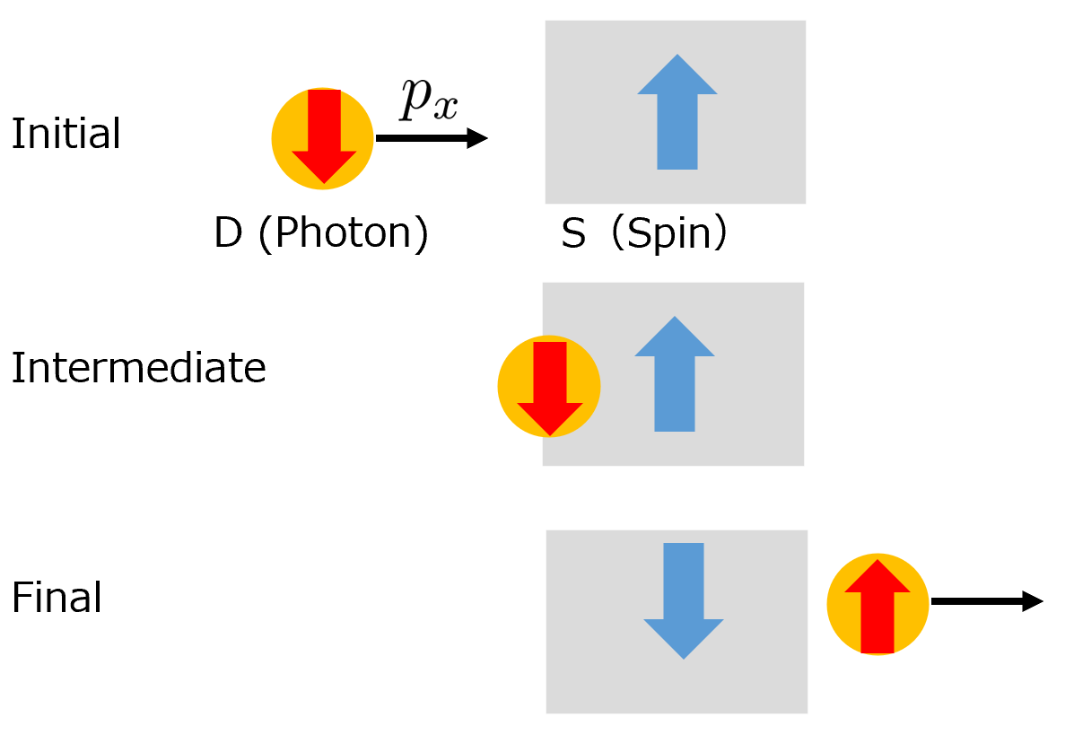
Figure 1: Conceptual figure of the setting.

We regard the implementation of SWAP gate as the measurement of a nuclear spin $\sigma_{z}$ where a meter observable is a photon spin $\sigma_{z}$ and use Eq. (14), then we find that

$$\epsilon(\sigma_{z})^{2}\geq\frac{b^{2}|\braket{\sigma_{y}}|^{2}}{b^{2}\sigma(\sigma_{x})^{2}+\sigma(p_{x})^{2}}$$ (18)

holds. Note that because $\sigma_{z,D}$ and $p_{x}$ are operators acting on different Hilbert spaces, the Yanase condition is satisfied. On the other hand, when we succeed in implementing SWAP gate $U_{SWAP}$ perfectly,

$$\epsilon(\sigma_{z})^{2}=\braket{[\sigma_{z,S}\otimes I_{D}-U_{SWAP}^{\dagger}(I_{S}\otimes\sigma_{z,D})U_{SWAP}]^{2}}=0$$ (19)

must be satisfied. Therefore, we are not able to implement SWAP gate perfectly when the fluctuation of momentum of the photon in the initial state is not infinity.

We are able to quantify it by deriving an inequality between the gate fidelity of SWAP gate $F_{SWAP}$ and the energy variance. Before showing the inequality of $F_{SWAP}$, we give the definition of the gate fidelity and the worst error probability of the physical realization. We consider that we would like to implement a unitary gate $U_{ideal}$ which acts on two systems $S$ and $A$. We represent the initial state of the composite system $S$+$A$ by $\rho$. We also consider an external system $E$ and suppose that its initial state is $\ket{\xi}$. Considering the purification, we are able to assume that the initial state of the external system is a pure state. We define a unitary time evolution operator which acts on the composite system of $S$+$A$+$E$ by $U$. The state of $S$+$A$ after $U$ is applied, which we represent by $\mathcal{E}(\rho)$, is

$$\mathcal{E}(\rho)={\rm Tr}_{E}[U(\rho\otimes\ket{\xi}\bra{\xi})U^{\dagger}].$$ (20)

On the other hand, if we succeed in implementing $U_{ideal}$ perfectly, the final state of $S$+$A$ is $U_{ideal}\rho U_{ideal}^{\dagger}$. Therefore, we define the worst error probability of the physical realization of $U_{ideal}$ by the CB distance as follows:

$$D_{CB}(\mathcal{E},U_{ideal})=\sup_{\rho_{S+A+E^{\prime}}}D\left(\mathcal{E}_{S+A}\otimes I_{E^{\prime}}(\rho_{S+A+E^{\prime}}),(U_{ideal}\otimes I_{E^{\prime}})\rho_{S+A+E^{\prime}}(U_{ideal}^{\dagger}\otimes I_{E^{\prime}})\right),$$ (21)

where $E^{\prime}$ is another external system and $D(\rho_{1},\rho_{2})$ is the trace distance given by

$$D(\rho_{1},\rho_{2})=\frac{1}{2}{\rm Tr}\left[|\rho_{1}-\rho_{2}|\right].$$ (22)

The gate trace distance between $U_{ideal}$ and the physical implementation $\mathcal{E}$, $D(\mathcal{E},U_{ideal})$ is defined by

$$D(\mathcal{E},U_{ideal})=\sup_{\rho_{S+A}}D(\mathcal{E}(\rho_{S+A}),U_{ideal}\,\rho_{S+A}U^{\dagger}_{ideal}).$$ (23)

From the definition of the CB distance,

$$D_{CB}(\mathcal{E},U_{ideal})\geq D(\mathcal{E},U_{ideal})$$ (24)

holds. By minimizing over all physical implementation $(U,\ket{\xi})$,

$$D_{CB}(\mathcal{E},U_{ideal})\geq\inf_{(U,\ket{\xi})}D(\mathcal{E},U_{ideal})$$ (25)

can be found. Because of the joint convexity of the trace distance, we are able to assume that $\rho_{S+A}$ is a pure state. The gate fidelity between $U_{ideal}$ and $\mathcal{E}$, which is denoted by $F(\mathcal{E},U_{ideal})$, is give by

$$F(\mathcal{E},U_{ideal})\coloneqq\inf_{\ket{\psi}}F(\ket{\psi}),$$ (26)

where

$$F(\ket{\psi})=\braket{\psi}{U_{ideal}^{\dagger}\mathcal{E}(\ket{\psi}\bra{\psi})U_{ideal}}{\psi}^{\frac{1}{2}}.$$ (27)

The following relation between the trace distance and fielity holds:

$$D(\mathcal{E},U_{ideal})\geq 1-F(\mathcal{E},U_{ideal})^{2}.$$ (28)

Therefore,

$$D_{CB}(\mathcal{E},U_{ideal})\geq D(\mathcal{E},U_{ideal})\geq 1-F(\mathcal{E},U_{ideal})^{2}$$ (29)

is verified. If $D_{CB}(\mathcal{E},U_{ideal})>0$, we are not able to implement $U_{ideal}$ perfectly.

When the hamiltonian is given by Eq. (17),

$$F_{SWAP}^{2}\leq 1-\frac{b^{2}}{4b^{2}+4\sigma(p_{x})^{2}}$$ (30)

holds. The derivation of this inequality is given in Appendix B.

Furthermore, we are able to extend the bound for the Hadamard gate under an additive conservation law in Ref. [20] to that under the energy conservation law. For example, let us consider we would like to implement the Hadamard gate using the composite system $S$+$D$ where the Hamiltonian of the composite system is

$$H=s_{x,S}+L_{x,D}+H_{int},$$ (31)

where $s_{x,S}$ and $L_{x,D}$ are the $x$ component of the angular momentum of each system. When the interaction term satisfies Eq. (8) , from Eq. (14) and similar calculations as in Ref. [20], we are able to show the following bound:

$$1-F_{H}^{2}\geq\epsilon(s_{z,S})^{2}\geq\frac{1}{4+16\sigma(L_{x,D})^{2}},$$ (32)

where $F_{H}$ is the gate fidelity of the Hadamard gate.

In this section, we show the relation Eq. (14) between the measurement error in scattering processes and the energy conservation. We also prove that SWAP gate is not able to be implemented perfectly as an application of Eq. (14). Futhermore, the bound of the gate fidelity of the Hadamard gate proved in Ref. [20] under an additive conservation law is able to be expanded under the energy conservation in scattering processes.

III Conditions which Hamiltonian of a controlled system must satisfy for implementing controlled unitary gates perfectly under energy conservation

In this section, we show necessary conditions that the Hamiltonian of a control system must satisfy for implementing controlled unitary gates with zero error in scattering processes under energy conservation. We also give an upper bound of the gate fidelity of two-qubit controlled gates.

Let us represent a control system and a target system as $C$ and $T$, respectively. We consider two orthogonal states of $C$, $\ket{\phi_{0}}_{C}$ and $\ket{\phi_{1}}_{C}$. We deal with a controlled gate $U_{CU}$ such that when the state of $C$ is $\ket{\phi_{0}}_{C}$, there is no effect on $T$, and when it is $\ket{\phi_{1}}_{C}$, a unitary operator $V_{T}$ is acting in $T$. The action of $U_{CU}$ is written as

$$U_{CU}\ket{\phi_{0}}_{C}\ket{\psi}_{T} = \ket{\phi_{0}^{\prime}}_{C}\ket{\psi}_{T},$$

$$U_{CU}\ket{\phi_{1}}_{C}\ket{\psi}_{T} = \ket{\phi_{1}^{\prime}}_{C}\left(V_{T}\ket{\psi}_{T}\right),$$ (33)

for an arbitrary state of $T$ $\ket{\psi}_{T}$. Note that final states of $C$, $\ket{\phi_{0}^{\prime}}_{C}$ and $\ket{\phi_{1}^{\prime}}_{C}$ are independent of the initial state of $T$, $\ket{\psi}_{T}$. We consider a non-trivial gate such that $V_{T}\neq I_{T}$.

Let $H_{C}$, $H_{T}$, and $H_{int}$ denote the Hamiltonian of $C$, that of $T$, and an interaction Hamiltonian between $C$ and $T$. The total Hamiltonian of the composite system $C$ and $T$, represented as $H_{C+T}$, is given by

$$H_{C+T}=H_{C}\otimes I_{T}+I_{C}\otimes H_{T}+H_{int}.$$ (34)

Like the previous section, we consider a scattering process in which $C$ and $T$ are initially spatially separated, and the interaction appears as $C$ approaches $T$. Some time later, $C$ and $T$ are spatially separated again. We assume that

$$\bra{\phi}_{C}\bra{\psi}_{T}H_{int}\ket{\phi}_{C}\ket{\psi}_{T}=0,$$ (35)

for an arbitrary superposition state of $C$, $\ket{\phi}_{C}=c_{0}\ket{\phi_{0}}_{C}+c_{1}\ket{\phi_{1}}_{C}$ where $|c_{0}|^{2}+|c_{1}|^{2}=1$, and an arbitrary state of $T$, $\ket{\psi}_{T}$. We set $\tau$ to the time when the non-zero interaction exists. The time evolution operator describing the scattering process $U_{CT}$ is written as

$$U_{CT}=\exp(-i\tau H_{C+T}).$$ (36)

When implementing the controlled unitary gate, $U_{CU}$ using this scattering process, we adjust the interaction $H_{int}$ and the interaction time $\tau$ to satisfy the following relations:

$$U_{CT}\ket{\phi_{0}}_{C}\ket{\psi}_{T} = \ket{\phi^{\prime}_{0}}_{C}\ket{\psi}_{T},$$

$$U_{CT}\ket{\phi_{1}}_{C}\ket{\psi}_{T} = \ket{\phi^{\prime}_{1}}_{C}(V_{T}\ket{\psi}_{T}),$$ (37)

for arbitrary initial state $\ket{\psi}_{T}$ in $T$. However when the energy conservation law

$$[H_{C+T},U_{CT}]=0,$$ (38)

exists, $H_{C}$ must satisfy the following initial condition,

$$\braket{\phi_{0}}{H_{C}}{\phi_{1}}_{C}=0$$ (39)

to implement the gate $U_{CU}$ with zero-error.

If $H_{int}$ fulfills the conditions below similar to conditions Eq. (8):

$$H_{int}\ket{\phi_{0}}_{C}\ket{\psi}_{T} = 0,$$

$$H_{int}\ket{\phi_{1}}_{C}\ket{\psi}_{T} = 0,$$

$$H_{int}\ket{\phi^{\prime}_{0}}_{C}\ket{\psi}_{T} = 0,$$

$$H_{int}\ket{\phi^{\prime}_{1}}_{C}\ket{\psi}_{T} = 0,$$ (40)

for an arbitrary state $\ket{\psi}_{T}$, the additional condition,

$$\braket{\phi_{0}}{H_{C}^{2}}{\phi_{1}}=0,$$ (41)

must be satisfied to implement $U_{CU}$ perfectly under energy conservation. We give proof of Eq. (39) and Eq. (41) in the appendix C.

Furthermore, if $C$ and $T$ are one-qubit systems, $U_{CU}$ becomes a two-qubit controlled gate, and $V_{T}$ becomes a one-qubit gate. $V_{T}$ can be represented as

$$V_{T}(\theta)=e^{i\phi}\left(\cos\frac{\theta}{2}I_{T}+i\sin\frac{\theta}{2}\vec{u}\cdot\vec{\sigma}\right),$$ (42)

where $\vec{u}$ is a three-dimensional real vector and $\vec{\sigma}$ is the vector defined by $\vec{\sigma}\coloneqq(\sigma_{x},\sigma_{y},\sigma_{z})$, where $\sigma_{x}$, $\sigma_{y}$and $\sigma_{z}$ are Pauli matrices which act on the Hilbert space of $T$. The domain of $\theta$ and $\phi$ are $0\leq\phi<2\pi$ and $0\leq\theta\leq\pi$, respectively.

When implementing a two-qubit controlled unitary gate $U_{CU}$ using a scattering process under energy conservation, we have the following inequality regarding the CB distance between $U_{CU}$ and the physical implementation $\mathcal{E}_{\alpha}$:

$$D_{CB}(\mathcal{E}_{\alpha},U_{CU})^{2}\geq\frac{\sin^{2}\frac{\theta}{2}\left\|\left[\sigma(\vec{l})_{C},H_{C}\right]\right\|^{2}}{16(2\gamma+\|H_{A}\|)^{2}}$$ (43)

where $\sigma(\vec{l})\coloneqq\ket{\phi_{0}}\bra{\phi_{0}}-\ket{\phi_{1}}\bra{\phi_{1}}$, $\gamma\coloneqq\max\{\|H_{S}\|,\|H_{T}\|\}$ and $H_{A}$ is the free Hamiltonian of the ancillary system $A$. If $\braket{\phi_{0}}{H_{C}}{\phi_{1}}=0$ holds, $H_{C}$ commutes with $\sigma(\vec{l})$ and the upper bound of gate fidelity is 1, that is to say, we can implement $U_{CU}$ perfectly. We also find that the bound dependence of the angle $\theta$ is $\sin^{2}\frac{\theta}{2}$. The derivation of Eq. (43) is provided in the appendix D.

In this section, we show that $H_{C}$ must satisfy Eq. (39) and Eq. (41) to implement a non-trivial controlled gate whose action is given by Eq.(33) with zero-error using scattering process under energy conservation law. We also obtain the upper bound of gate fidelity Eq. (43) for a two-qubit controlled gate.

IV Summary

We showed a lower bound of the measurement error Eq. (14) for scattering-type measurements which satisfy Eq. (8) under the energy conservation in section 2. In section 2 we also presented that the SWAP gate is not able to be implemented perfectly as an application of Eq. (14). Futhermore, the bound of the gate fidelity of the Hadamard gate proved in Ref. [20] under an additive conservation law is able to be expanded under the energy conservation in scattering processes. In section 3, we gived the necessary condition Eq. (39) which must be fulfilled to implement a controlled unitary gate described by Eq. (33) without error in a scattering process under energy conservation. We also proved that when the interaction term satisfies Eq. (40), the additional necessary condition for $H_{C}$, Eq. (41) must also be fulfilled to implement a controlled unitary gate perfectly. Moreover, when $C$ and $T$ are one-qubit systems, the quantitative relation Eq. (43) between the gate fidelity and the non-diagonal entry of $H_{C}$ is shown. This result extends Ozawa’s result which evaluates the upper bound of the gate fidelity of CNOT gates [21].

Appendix A Proof of bound of error of scattering-type measurement under energy conservation

In this section, we derive the inequality of the measurement error in a scattering process under energy conservation Eq. (14). We introduce another measuring device which is a particle moving in one dimension. We represent this particle by $A$. Let the position and the momentum of $A$ be $Q_{A}$ and $P_{A}$, respectively. And suppose that $A$ and $D$ have an interaction described by

$$H^{\prime}_{int}=kI_{S}\otimes M_{D}\otimes P_{A},$$ (44)

between $\tau$ and $\tau^{\prime}$, where $k\coloneqq\frac{1}{\tau^{\prime}-\tau}$. Except for this time window between $\tau$ and $\tau^{\prime}$, we suppose that there is no interaction between $A$ and $S$+$D$. The hamiltonian of the composite system $S$+$D$+$A$, $H_{S+D+A}$ is given by

$$H_{S+D+A}=H_{S+D}+H_{A}+H^{\prime}_{int},$$ (45)

between time $\tau$ and $\tau^{\prime}$, where $H_{A}$ is the free Hamiltonian of $A$. Note that the interaction between $S$ and $D$, $H_{int}$, is 0 after $\tau$.

We consider the indirect measurement of $M_{D}$ by measuring $Q_{A}$ and assume that the period when the interaction $H_{int}^{\prime}$ exists, $\tau^{\prime}-\tau$, is very short. In this assumption, $H_{int}^{\prime}$ is very large compared to the free Hamiltonian of $S$+$D$+$A$, so $H_{int}^{\prime}$ can be regarded as the total Hamiltonian in the time window from $\tau$ to $\tau^{\prime}$.

We denote by $U^{\prime}_{S+D+A}$ the time evolution operator between $\tau$ and $\tau^{\prime}$. $U^{\prime}_{S+D+A}$ is given by

$$U^{\prime}_{S+D+A}=e^{-i(I_{S}\otimes M_{D}\otimes P_{A})}.$$ (46)

On the other hand, the time evolution of $A$ between 0 and $\tau$, $U_{A}$, is represented by

$$U_{A}=e^{-iH_{A}\tau}.$$ (47)

The time evolution operator of the composite system $S$+$D$+$A$ between the initial time $t=0$ to the final time $t=\tau+\tau^{\prime}$ expressed as $U_{S+D+A}$ is

$$U_{S+D+A}=U^{\prime}_{S+D+A}(U_{S+D}\otimes U_{A}).$$ (48)

Next, we define the error $\alpha$ of measuring $\tilde{M_{D}}\coloneqq I_{S}\otimes M_{D}\otimes I_{A}$ at $\tau$ by measuring $\tilde{Q_{A}}\coloneqq I_{S}\otimes I_{D}\otimes Q_{A}$ at $\tau^{\prime}$ and we define by $\beta$ the error of measuring $\tilde{A_{S}}\coloneqq A_{S}\otimes I_{D}\otimes I_{A}$ at $t=0$ by measuring $\tilde{Q_{A}}$ at $\tau^{\prime}$. $\alpha$ and $\beta$ are written as

$$\alpha = \left\|[U^{\prime\dagger}_{S+D+A}\tilde{Q_{A}}U^{\prime}_{S+D+A}-\tilde{M_{D}}]\left(U_{S+D}\ket{\psi}_{S}\ket{\xi}_{D}\right)U_{A}\ket{\zeta}_{A}\right\|,$$ (49)

$$\beta = \left\|[U^{\dagger}_{S+D+A}\tilde{Q}_{A}U_{S+D+A}-\tilde{A}_{S}]\ket{\psi}_{S}\ket{\xi}_{D}\ket{\zeta}_{A}\right\|,$$ (50)

where $\ket{\zeta}_{A}$ is the initial state of $A$.

To evaluate $\epsilon(A_{S})$ given in Eq. (13), we first consider the Ozawa inequality in the measurement $\tilde{A}_{S}$ using $\tilde{Q}_{A}$:

$$\beta\eta(H_{0})+\beta\sigma(H_{0})+\sigma(\tilde{A_{S}})\eta(H_{0})\geq\frac{1}{2}\left|\Braket{[\tilde{A_{S}},H_{0}]}\right|,$$ (51)

where $H_{0}\coloneqq H_{S}\otimes I_{D}\otimes I_{A}+I_{S}\otimes H_{D}\otimes I_{A}$ is the free Hamiltonian of the composite system $S$+$D$ and $\eta(H_{0})$ is the disturbance of $H_{0}$ by the measurement, which is given by

$$\eta(H_{0})=\left\|[U_{S+D+A}^{\dagger}H_{0}U_{S+D+A}-H_{0}]\ket{\psi}_{S}\ket{\xi}_{D}\ket{\zeta}_{A}\right\|.$$ (52)

For an observable $O$, $\sigma(O)$ represents the standard deviation of $O$ in the initial state.

From the Baker-Campbell-Hausdorff formula,

$$U^{\prime\dagger}_{S+D+A}\tilde{Q_{A}}U^{\prime}_{S+D+A}=\tilde{Q_{A}}+\tilde{M_{D}}$$ (53)

holds. Then we can calculate $\alpha$ as

$$\alpha = \left\|Q_{A}U_{A}\ket{\zeta}_{A}\right\|.$$ (54)

Looking at Eq. (54), we find that the error of measuring $M_{D}$ by $Q_{A}$ is given by the square root of the expectation value of $Q_{A}^{2}$ on the final state of $A$. Therefore, for any $\epsilon>0$, we can impose $\alpha<\epsilon$ by choosing $\ket{\zeta}_{A}$ appropriately. Since $M_{D}$ is a conserved quantity during measurement which is described by $U^{\prime}_{S+D+A}$, $[U^{\prime}_{S+D+A},\tilde{M_{D}}]=0$ holds, and we also find the following relation:

$$\alpha = \left\|[U^{\dagger}_{S+D+A}\tilde{Q_{A}}U_{S+D+A}-U^{\dagger}_{S+D+A}\tilde{M_{D}}U_{S+D+A}]\ket{\psi}_{S}\ket{\xi}_{D}\ket{\zeta}_{A}\right\|.$$ (55)

Next, we derive the relation between $\alpha$, $\beta$ and $\epsilon(A_{S})$. $\epsilon(A_{S})$ is deformed as

$$\epsilon(A_{S}) = \left\|[U^{\dagger}_{S+D+A}\tilde{M_{D}}U_{S+D+A}-\tilde{A_{S}}]\ket{\psi}_{S}\ket{\xi}_{D}\ket{\zeta}_{A}\right\|,$$ (56)

where we used $[\tilde{M_{D}},U^{\prime}_{S+D+A}]=0$. From Eq. (55), Eq. (56) and the triangle inequality, we obtain the following relation:

$$\beta \leq \alpha+\epsilon(A_{S}).$$ (57)

We evaluate the disturbance $\eta(H_{0})$. From the Yanase condition $[H_{D},M_{D}]=0$, we have $[U^{\prime}_{S+D+A},H_{0}]=0$, which means that $H_{0}$ is unchanged during the measurement using $A$. Then we obtain

$$\eta(H_{0}) = \left\|[U_{S+D}^{\dagger}H_{0}U_{S+D}-H_{0}]\ket{\psi}_{S}\ket{\xi}_{D}\ket{\zeta}_{A}\right\|$$ (58)

$$= \left\|[U_{S+D}^{\dagger}H_{int}U_{S+D}-H_{int}]\ket{\psi}_{S}\ket{\xi}_{D}\right\|$$

$$= 0.$$

In the first line, we used that $H_{0}$ is conserved during measurement using $A$. The fact that $H_{S+D}$ is conserved during measurement using $D$ is utilized in the second line. In the final line, the assumption Eq. (8) is considered. From Eq. (51), Eq. (57) and Eq. (58),

$$(\alpha+\epsilon(A_{S}))\sigma(H_{0})\geq\frac{1}{2}\left|\Braket{[\tilde{A_{S}},H_{0}]}\right|$$ (59)

is shown. Because $\alpha$ can be arbitrarily small by choosing $\ket{\zeta}_{A}$ appropriately,

$$\epsilon(A_{S})\sigma(H_{0})\geq\frac{1}{2}\left|\Braket{[\tilde{A_{S}},H_{0}]}\right|$$ (60)

holds. Taking $[\tilde{A}_{S},H_{0}]=[A_{S},H_{S}]$ and $\sigma(H_{0})^{2}=\sigma(H_{S})^{2}+\sigma(H_{D})^{2}$ into account, we get

$$\epsilon(A_{S})^{2}\geq\frac{\left|\Braket{[A_{S},H_{S}]}\right|^{2}}{4\sigma(H_{S})^{2}+4\sigma(H_{D})^{2}},$$ (61)

and Eq. (14) is proved.

Before closing this section, we comment on a bound of the measurement error when we assume the weak Yanase condition $[U^{\dagger}_{S+D}(I_{S}\otimes M_{D})U_{S+D},H_{S+D}]=0$ instead of the Yanase condition $[H_{D},M_{D}]=0$. Tukiainen proved that if $[U^{\dagger}_{S+D}(I_{S}\otimes M_{D})U_{S+D},H_{S+D}]=0$ is satisfied in a repeatable measurement of $A_{S}$, then $[A_{S},\braket{\xi}{H_{S+D}}{\xi}]=0$ holds [49]. We are able to quantify it by the similar proof of Eq. (14). We consider the following Ozawa inequality instead of Eq. (51):

$$\beta\eta(H_{S+D})+\beta\sigma(H_{S+D})+\sigma(\tilde{A}_{S})\eta(H_{S+D})\geq\frac{1}{2}\left|\Braket{[\tilde{A}_{S},H_{S+D}]}\right|=\frac{1}{2}\left|\bra{\psi}_{S}[A_{S},\bra{\xi}_{D}H_{S+D}\ket{\xi}_{D}]\ket{\psi}_{S}\right|.$$

When the weak Yanase condition is satisfied, we are able to show that $\eta(H_{S+D})=0$ as follows:

$$\eta(H_{S+D}) = \left\|[U_{S+D+A}^{\dagger}H_{S+D}U_{S+D+A}-H_{S+D}]\ket{\psi}_{S}\ket{\xi}_{D}\ket{\zeta}_{A}\right\|$$ (63)

$$= \left\|[U_{S+D}^{\dagger}H_{S+D}U_{S+D}-H_{S+D}]\ket{\psi}_{S}\ket{\xi}_{D}\ket{\zeta}_{A}\right\|$$ (64)

$$= 0,$$ (65)

where in the second line, we used $[M_{D},H_{S+D}]=0$ which is obtained from the weak Yanase condition and the energy conservation law because $[U^{\dagger}_{S+D}(I_{S}\otimes M_{D})U_{S+D},H_{S+D}]=U^{\dagger}_{S+D}[I_{S}\otimes M_{D},H_{S+D}]U_{S+D}=0$ holds. In the third line, the energy conservation law is considered. From Eq. (57), Eq. (A) and $\eta(H_{S+D})=0$ and setting $\alpha$ to be arbitrarily small, we find that

$$\epsilon(A_{S})^{2}\geq\frac{\left|\bra{\psi}_{S}[A_{S},\bra{\xi}_{D}H_{S+D}\ket{\xi}_{D}]\ket{\psi}_{S}\right|^{2}}{4\sigma(H_{S+D})^{2}}$$ (66)

holds.

In this section, we considered the scattering-type measurements in which the interaction vanishes when the detector and system are spatially separated under energy conservation. We derived the lower bound of measurement error Eq. (14) for this type of measurement.

Appendix B Upper bound of the gate fidelity of SWAP gate

In this section, we derive the inequality (30) between the gate fidelity of SWAP gate $F_{SWAP}$ and the energy variance. We first give a relation between the measurement error $\epsilon(\sigma_{z})$ and $F_{SWAP}$. Then we prove an upper bound of $F_{SWAP}$ using it and Eq. (18).

Firstly, we write the act of $U$ in Eq. (20) as

$$U\ket{a}_{S}\ket{b}_{A}\ket{\xi}_{E}=\sum_{j,k=0}^{1}\ket{j}_{S}\ket{k}_{A}\ket{E_{j,k}^{a,b}}_{E}.$$ (67)

$a$ and $b$ take 0 or 1. $\{\ket{0},\ket{1}\}$ represents the computational basis states. From the orthonormality of the initial state,

$$\delta_{ac}\delta_{bd} = \braket{a,b}{c,d}=\braket{a,b,\xi}{U^{\dagger}U}{c,d,\xi}=\sum_{j,k=0}^{1}\braket{E_{j,k}^{a,b}}{E_{j,k}^{c,d}}$$ (68)

holds. When the initial state of $S$+$A$ is $\ket{\alpha,\beta}\,(\alpha,\beta=0,1)$, the state after the time evolution described by $U$ is given by

$$\mathcal{E}(\ket{\alpha,\beta}\bra{\alpha,\beta}) = \sum_{j,k,l,m}\ket{j,k}\bra{l,m}\braket{E_{l,m}^{\alpha,\beta}}{E_{j,k}^{\alpha,\beta}}.$$ (69)

Therefore, the squared of $F(\ket{\alpha,\beta})$ for SWAP gate is written as follows:

$$F(\ket{\alpha,\beta})^{2} = \braket{E_{\beta,\alpha}^{\alpha,\beta}}{E_{\beta,\alpha}^{\alpha,\beta}}.$$ (70)

Next, let us represent the measurement error $\epsilon(\sigma_{z})$ using $\ket{E^{a,b}_{c,d}}$. We suppose that the initial state of $S$+$A$ is $\ket{\psi}=\sum_{\alpha,\beta=0}^{1}c_{\alpha,\beta}\ket{\alpha,\beta}$. We find that

$$\epsilon(\sigma_{z})^{2} = \|\left[(I_{S}\otimes\sigma_{z,A}\otimes I_{E})U-U(\sigma_{z,S}\otimes I_{A}\otimes I_{E})\right]\ket{\psi}_{S+A}\ket{\xi}_{E}\|^{2}$$ (71)

$$= 4\left\|\sum_{\beta}c_{1,\beta}\ket{E_{0,0}^{1,\beta}}\right\|^{2}+4\left\|\sum_{\beta}c_{1,\beta}\ket{E_{1,0}^{1,\beta}}\right\|^{2}+4\left\|\sum_{\beta}c_{0,\beta}\ket{E_{0,1}^{0,\beta}}\right\|^{2}+4\left\|\sum_{\beta}c_{0,\beta}\ket{E_{1,1}^{0,\beta}}\right\|^{2}$$ (72)

holds. We rewrite it by the gate fidelity. In the following, we represent $F(\mathcal{E},U_{SWAP})$ by $F_{SWAP}$. The following relations hold:

$$\epsilon(\sigma_{z})^{2} = 4\left\{|c_{1,0}|^{2}\left(1-\left\|\ket{E_{0,1}^{1,0}}\right\|^{2}-\left\|\ket{E_{1,1}^{1,0}}\right\|^{2}\right)+|c_{0,0}|^{2}\left(1-\left\|\ket{E_{0,0}^{0,0}}\right\|^{2}-\left\|\ket{E_{1,0}^{0,0}}\right\|^{2}\right)\right.$$ (76)

$$+2{\rm Re}\left[c_{1,0}c_{1,1}^{*}\left(\braket{E_{0,0}^{1,1}}{E_{0,0}^{1,0}}+\braket{E_{1,0}^{1,1}}{E_{1,0}^{1,0}}\right)+c_{0,0}c_{0,1}^{*}\left(\braket{E_{0,1}^{0,1}}{E_{0,1}^{0,0}}+\braket{E_{1,1}^{0,1}}{E_{1,1}^{0,0}}\right)\right]$$

$$+\left.|c_{1,1}|^{2}\left(1-\left\|\ket{E_{0,1}^{1,1}}\right\|^{2}-\left\|\ket{E_{1,1}^{1,1}}\right\|^{2}\right)+|c_{0,1}|^{2}\left(1-\left\|\ket{E_{0,0}^{0,1}}\right\|^{2}-\left\|\ket{E_{1,0}^{0,1}}\right\|^{2}\right)\right\}$$

$$\leq 4\left\{|c_{1,0}|^{2}\left(1-F(\ket{1,0})^{2}\right)+|c_{0,0}|^{2}\left(1-F(\ket{0,0})^{2}\right)\right.$$

$$+2\left|c_{1,0}c_{1,1}^{*}\left(\braket{E_{0,0}^{1,1}}{E_{0,0}^{1,0}}+\braket{E_{1,0}^{1,1}}{E_{1,0}^{1,0}}\right)+c_{0,0}c_{0,1}^{*}\left(\braket{E_{0,1}^{0,1}}{E_{0,1}^{0,0}}+\braket{E_{1,1}^{0,1}}{E_{1,1}^{0,0}}\right)\right|$$

$$+\left.|c_{1,1}|^{2}\left(1-F(\ket{1,1})^{2}\right)+|c_{0,1}|^{2}\left(1-F(\ket{0,1})^{2}\right)\right\}$$

$$\leq 4\left\{1-F_{SWAP}^{2}+2|c_{1,0}||c_{1,1}|\left(\left\|\ket{E_{0,0}^{1,1}}\right\|\left\|\ket{E_{0,0}^{1,0}}\right\|+\left\|\ket{E_{1,0}^{1,1}}\right\|\left\|\ket{E_{1,0}^{1,0}}\right\|\right)\right.$$

$$\left.+2|c_{0,0}||c_{0,1}|\left(\left\|\ket{E_{0,1}^{0,1}}\right\|\left\|\ket{E_{0,1}^{0,0}}\right\|+\left\|\ket{E_{1,1}^{0,1}}\right\|\left\|\ket{E_{1,1}^{0,0}}\right\|\right)\right\}$$

$$\leq 4\left\{1-F_{SWAP}^{2}+|c_{1,0}||c_{1,1}|\left(\left\|\ket{E_{0,0}^{1,1}}\right\|^{2}+\left\|\ket{E_{0,0}^{1,0}}\right\|^{2}+\left\|\ket{E_{1,0}^{1,1}}\right\|^{2}+\left\|\ket{E_{1,0}^{1,0}}\right\|^{2}\right)\right.$$

$$\left.+|c_{0,0}||c_{0,1}|\left(\left\|\ket{E_{0,1}^{0,1}}\right\|^{2}+\left\|\ket{E_{0,1}^{0,0}}\right\|^{2}+\left\|\ket{E_{1,1}^{0,1}}\right\|^{2}+\left\|\ket{E_{1,1}^{0,0}}\right\|^{2}\right)\right\}$$

$$\leq 4(1-F_{SWAP}^{2})\left[1+2(|c_{1,0}||c_{1,1}|+|c_{0,0}||c_{0,1}|)\right].$$ (77)

In the first line, Eq. (68) is used. In second line, we considered Eq. (70). In the third line, the triangle inequality and the Cauchy-Schwarz inequality are applied. In the fourth line, the relation between the mean square and the geometric mean is taken into consideration. In the seventh line, we used Eq. (68) and Eq. (70).

When the hamiltonian is given by as Eq.(17), Eq. (18) holds and

$$4(1-F_{SWAP}^{2})\left[1+2(|c_{1,0}||c_{1,1}|+|c_{0,0}||c_{0,1}|)\right]\geq\frac{b^{2}|\braket{\sigma_{y,S}}|^{2}}{b^{2}\sigma(\sigma_{x,S})^{2}+\sigma(p_{x})^{2}}$$ (78)

can be proved. Let us maximize the right-hand side over states of $S$+$A$. Because the right-hand side is independent of states of $A$, we consider maximizing over the system’s pure state. It is denoted by $d_{0}\ket{0}+d_{1}\ket{1}$. Then we find that

$$\frac{b^{2}|\braket{\sigma_{y,S}}|^{2}}{b^{2}\sigma(\sigma_{x,S})^{2}+\sigma(p_{x})^{2}} = \frac{4b^{2}|{\rm Im}(d_{0}d_{1}^{*})|^{2}}{b^{2}(1-4|{\rm Re}(d_{0}d_{1}^{*})|^{2})+\sigma(p_{x})^{2}}.$$ (79)

Because

$$|{\rm Re}(d_{0}d_{1}^{*})|^{2}+|{\rm Im}(d_{0}d_{1}^{*})|^{2}=|d_{0}d_{1}^{*}|^{2}\leq\left(\frac{|d_{0}|^{2}+|d_{1}|^{2}}{2}\right)^{2}=\frac{1}{4}$$ (80)

holds, we make the change of variales $|{\rm Re}(d_{0}d_{1}^{*})|=r\cos\theta$, $|{\rm Im}(d_{0}d_{1}^{*})|=r\sin\theta$, where $0\leq r\leq\frac{1}{2}$,$0\leq\theta<2\pi$. We introduce a function $G(r,\theta)$ as follows:

$$G(r,\theta)=\frac{b^{2}|\braket{\sigma_{y,S}}|^{2}}{b^{2}\sigma(\sigma_{x,S})^{2}+\sigma(p_{x})^{2}} = \frac{4b^{2}r^{2}\sin^{2}\theta}{b^{2}(1-4r^{2}\cos^{2}\theta)+\sigma(p_{x})^{2}}.$$ (81)

The derivative of it is

$$\frac{\partial G(r,\theta)}{\partial\theta}=\frac{4b^{2}r^{2}\sin 2\theta\left[b^{2}(1-4r^{2})+\sigma(p_{x})^{2}\right]}{\left[b^{2}(1-4r^{2}\cos^{2}\theta)+\sigma(p_{x})^{2}\right]^{2}}.$$ (82)

Since $\left[b^{2}(1-4r^{2})+\sigma(p_{x})^{2}\right]\geq 0$ holds, $G(r,\theta)$ takes the maximum value at $\theta=\frac{\pi}{2}$ and $\frac{3\pi}{2}$ for a fixed $r$. Because $G\left(r,\frac{\pi}{2}\right)=G\left(r,\frac{3\pi}{2}\right)=\frac{4b^{2}r^{2}}{b^{2}+\sigma(p_{x})^{2}}$, the maximum value of $G(r,\theta)$ is $\frac{b^{2}}{b^{2}+\sigma(p_{x})^{2}}$, which is attained at $(r,\theta)=\left(\frac{1}{2},\frac{\pi}{2}\right)=\left(\frac{1}{2},\frac{3\pi}{2}\right)$. The eigenstates of $\sigma_{y,S}$ correspond to this case.

On the other hand, the coefficient of the left-hand side of Eq. (78), $1+2(|c_{1,0}||c_{1,1}|+|c_{0,0}||c_{0,1}|)$, takes the minimum value 1 when $S$’s state is the eigenstate of $\sigma_{y,S}$ and $A$’s state is $\ket{0}$. Hence, Eq. (30) is derived. On the other hand, because $p_{x}$ is an unbounded operator, the CB distance is 0. However if the variance of $p_{x}$ on the initial state is finite, from Eq. (30), we find that the implementation error occurs.

In this section, we proved the inequality Eq. (30) between the gate fidelity of SWAP gate and the energy variance as an application of Eq. (14).

Appendix C Proof of conditions which have to be fulfilled for implementing a controlled unitary gate perfectly

In this section, we prove the necessary condition Eq. (39) and Eq. (41) to implement a controlled gate described in Eq. (33) without error under energy conservation law.

Firstly, note that final states of $C$, $\ket{\phi_{0}^{\prime}}_{C}$ and $\ket{\phi_{1}^{\prime}}_{C}$, are independent of the initial state of $T$, $\ket{\psi}_{T}$ in Eq. (33), and two final states of $C$ are orthogonal to each other when we succeed in implementing $U_{CU}$ without error. The calculation to prove it is the same as in [55] in which Nielsen and Chuang proved the no-programming theorem.

Next we prove that

$$\bra{\phi_{0}}_{C}\bra{\psi_{0}}_{T}H_{int}\ket{\phi_{1}}_{C}\ket{\psi_{1}}_{T}=0$$ (83)

is valid under the assumption Eq. (35). Substituting $\ket{\phi}_{C}=c_{0}\ket{\phi_{0}}_{C}+c_{1}\ket{\phi_{1}}_{C}$ into Eq. (35),

$$2{\rm Re}\left[c_{0}^{*}c_{1}\bra{\phi_{0}}_{C}\bra{\psi}_{T}H_{int}\ket{\phi_{1}}_{C}\ket{\psi}_{T}\right]=0$$ (84)

is obtained. Since Eq. (84) holds for arbitrary complex numbers $c_{0}$ and $c_{1}$ such that $|c_{0}|^{2}+|c_{1}|^{2}=1$, we get

$$\bra{\phi_{0}}_{C}\bra{\psi}_{T}H_{int}\ket{\phi_{1}}_{C}\ket{\psi}_{T}=0.$$ (85)

Similarly, since Eq. (85) holds for an arbitrary state of $T$, $\ket{\psi}_{T}=d_{0}\ket{\psi_{0}}_{T}+d_{1}\ket{\psi_{1}}_{T}$, where $d_{0}$ and $d_{1}$ are arbitrary complex numbers which satisfy $|d_{0}|^{2}+|d_{1}|^{2}=1$,

$$d_{0}^{*}d_{1}\bra{\phi_{0}}_{C}\bra{\psi_{0}}_{T}H_{int}\ket{\phi_{1}}_{C}\ket{\psi_{1}}_{T}+d_{0}d_{1}^{*}\bra{\phi_{0}}_{C}\bra{\psi_{1}}_{T}H_{int}\ket{\phi_{1}}_{C}\ket{\psi_{0}}_{T}=0$$ (86)

can be shown. Considering $d_{0}=d_{1}=\frac{1}{\sqrt{2}}$, we find that

$$\bra{\phi_{0}}_{C}\bra{\psi_{0}}_{T}H_{int}\ket{\phi_{1}}_{C}\ket{\psi_{1}}_{T}+\bra{\phi_{0}}_{C}\bra{\psi_{1}}_{T}H_{int}\ket{\phi_{1}}_{C}\ket{\psi_{0}}_{T} = 0.$$ (87)

On the other hand, we get

$$\bra{\phi_{0}}_{C}\bra{\psi_{0}}_{T}H_{int}\ket{\phi_{1}}_{C}\ket{\psi_{1}}_{T}-\bra{\phi_{0}}_{C}\bra{\psi_{1}}_{T}H_{int}\ket{\phi_{1}}_{C}\ket{\psi_{0}}_{T} = 0$$ (88)

when substituting $d_{0}=\frac{1}{\sqrt{2}}$ and $d_{1}=\frac{i}{\sqrt{2}}$ into Eq. (86). By combining Eq. (87) with Eq. (88), we obtain Eq. (83). Furthermore, by substituting $\ket{\psi_{0}}_{T}=\ket{\psi}_{T}$ and $\ket{\psi_{1}}_{T}=V_{T}\ket{\psi}_{T}$, where $\ket{\psi}_{T}$ is an arbitrary initial state of $T$, and $\ket{\phi_{0}}_{C}=\ket{\phi_{0}^{\prime}}_{C}$ and $\ket{\phi_{1}}_{C}=\ket{\phi_{1}^{\prime}}_{C}$ into Eq. (83),

$$0 = \bra{\phi_{0}^{\prime}}_{C}\bra{\psi}_{T}H_{int}\ket{\phi_{1}^{\prime}}_{C}(V_{T}\ket{\psi}_{T})=\bra{\phi_{0}}_{C}\bra{\psi}_{T}U_{CU}^{\dagger}H_{int}U_{CU}\ket{\phi_{1}}_{C}\ket{\psi}_{T}$$ (89)

can be shown.

Based on the above facts, we derive Eq. (39). From the orthogonality of $\ket{\phi_{0}}$ and $\ket{\phi_{1}}$,

$$\braket{\phi_{0}}{H_{C}}{\phi_{1}}_{C}=\bra{\phi_{0}}_{C}\bra{\psi}_{T}(H_{T}+H_{C})\ket{\phi_{1}}_{C}\ket{\psi}_{T}$$ (90)

is obtained. By combining Eq. (90) with Eq. (85), we get

$$\braket{\phi_{0}}{H_{C}}{\phi_{1}}_{C}=\bra{\phi_{0}}_{C}\bra{\psi}_{T}(H_{T}+H_{C}+H_{int})\ket{\phi_{1}}_{C}\ket{\psi}_{T}.$$ (91)

Using Eq. (91) and the energy conservation law

$$[H_{C+T},U_{CU}]=0,$$ (92)

we find that

$$\braket{\phi_{0}}{H_{C}}{\phi_{1}}_{C} = \bra{\phi_{0}}_{C}\bra{\psi}_{T}U_{CU}^{\dagger}(H_{T}+H_{C}+H_{int})U_{CU}\ket{\phi_{1}}_{C}\ket{\psi}_{T}$$ (93)

$$= \bra{\phi_{0}^{\prime}}_{C}\bra{\psi}_{T}(H_{T}+H_{C}+H_{int})\ket{\phi_{1}^{\prime}}_{C}(V_{T}\ket{\psi}_{T})$$

holds. In addition to this, from $\braket{\phi_{0}^{\prime}}{\phi_{1}^{\prime}}=0$ and Eq. (89),

$$\braket{\phi_{0}}{H_{C}}{\phi_{1}}_{C}=\braket{\phi^{\prime}_{0}}{H_{C}}{\phi^{\prime}_{1}}_{C}\braket{\psi}{V_{T}}{\psi}_{T}$$ (94)

is able to be proved for any $\ket{\psi}_{T}$.

If $\braket{\phi_{0}}{H_{C}}{\phi_{1}}_{C}\neq 0$ holds, $\braket{\phi^{\prime}_{0}}{H_{C}}{\phi^{\prime}_{1}}_{C}\neq 0$ is obtained because $V_{T}\neq 0$. Therefore, from Eq. (94), we can calculate as follows:

$$\braket{\psi}{V_{T}}{\psi}_{T}=\frac{\braket{\phi_{0}}{H_{C}}{\phi_{1}}_{C}}{\braket{\phi^{\prime}_{0}}{H_{C}}{\phi^{\prime}_{1}}_{C}}.$$ (95)

Let the spectrum decomposition of $V_{T}$ be

$$V_{T}=\sum_{i}\alpha_{i}\ket{i}\bra{i},$$ (96)

where $\alpha_{i}$ is the $i$-th eigenvalue and $\ket{i}$ is the corresponding eigenvector.

By substituting $\ket{\psi}=\ket{i}$ into Eq. (95), we find that

$$\braket{i}{V_{T}}{i}_{T}=\alpha_{i}=\frac{\braket{\phi_{0}}{H_{C}}{\phi_{1}}_{C}}{\braket{\phi^{\prime}_{0}}{H_{C}}{\phi^{\prime}_{1}}_{C}}$$ (97)

holds for any $i$. Hence,

$$V_{T} = \frac{\braket{\phi_{0}}{H_{C}}{\phi_{1}}_{C}}{\braket{\phi^{\prime}_{0}}{H_{C}}{\phi^{\prime}_{1}}_{C}}I_{T}$$ (98)

is obtained. Since $V_{T}$ is a unitary operator, the following relation is valid:

$$\braket{\phi_{0}}{H_{C}}{\phi_{1}}_{C}=\braket{\phi^{\prime}_{0}}{H_{C}}{\phi^{\prime}_{1}}_{C}e^{i\delta},$$ (99)

where $\delta$ is a real number. When $\braket{\phi_{0}}{H_{C}}{\phi_{1}}_{C}\neq 0$, by taking Eq. (98) and Eq. (99) into account,

$$V_{T}=e^{i\delta}I_{T}$$ (100)

must hold. Therefore, when we want to implement a non-trivial controlled unitary gate like a CNOT gate without error under energy conservation, we proved that Eq. (39) has to be satisfied.

Next, we derive Eq. (41) under the assumption Eq. (40). A calculation similar to the derivation of Eq. (94) shows that

$$\braket{\phi_{0}}{H_{C}^{2}}{\phi_{1}}_{C} = \bra{\phi_{0}}_{C}\bra{\psi}_{T}(H_{C}^{2}+H_{T}^{2})\ket{\phi_{1}}_{C}\ket{\psi}_{T}$$ (101)

$$= \bra{\phi_{0}}_{C}\bra{\psi}_{T}[(H_{C}+H_{T}+H_{int})^{2}-2H_{C}\otimes H_{T}]\ket{\phi_{1}}_{C}\ket{\psi}_{T}$$

$$= \bra{\phi_{0}}_{C}\bra{\psi}_{T}[U_{CU}^{\dagger}(H_{C}+H_{T}+H_{int})^{2}U_{CU}-2H_{C}\otimes H_{T}]\ket{\phi_{1}}_{C}\ket{\psi}_{T}$$

$$= \bra{\phi^{\prime}_{0}}_{C}\bra{\psi}_{T}(H_{C}+H_{T})^{2}\ket{\phi^{\prime}_{1}}_{C}(V_{T}\ket{\psi}_{T})-2\braket{\phi_{0}}{H_{C}}{\phi_{1}}_{C}\braket{\psi}{H_{T}}{\psi}_{T}$$

$$= \braket{\phi^{\prime}_{0}}{H_{C}^{2}}{\phi^{\prime}_{1}}_{C}\braket{\psi}{V_{T}}{\psi}_{T}$$

is valid for any $\ket{\psi}_{T}$. In the first line, we used $\braket{\phi_{0}}{\phi_{1}}=0$. We applied Eq. (40) to the second line. In the third line, the energy conservation is considered. In the fourth line, Eq. (40) and Eq. (33) are utilized. The final line is derived by combining $\braket{\phi_{0}^{\prime}}{\phi_{1}^{\prime}}=0$ and Eq. (39) with Eq. (94).

If $\braket{\phi_{0}}{H_{C}^{2}}{\phi_{1}}\neq 0$ works, we are able to prove that $V_{T}$ must be proportional to $I_{T}$ by a calculation similar to the derivation of Eq. (100). Thus, we find that if the assumption Eq. (40) holds, Eq. (41) has to be fulfilled in addition to Eq. (39) to implement a non-trivial controlled unitary gate perfectly under energy conservation.

Appendix D Proof of upper bound of the gate fidelity of two qubits controlled unitary gate

In this section, we prove the upper bound of the gate fidelity of a two-qubits controlled unitary gate Eq. (43). In the following, we denote a three-dimensional real vector which is orthogonal to $\vec{u}$, where $\vec{u}$ is given in Eq. (42), by $\vec{v}$. There are two vectors orthogonal to $\vec{u}$, we set $\vec{v}$ to the vector which faces the $z$-axis positive when we rotate $\vec{u}$ so that it faces the $x$-axis positive. We define $\sigma(\vec{v})$ by $\sigma(\vec{v})\coloneqq\vec{v}\cdot\vec{\sigma}$. Let us denote the eigenvector with eigenvalue 1 and the eigenvector with eigenvalue -1 by $\ket{\chi_{0}}$ and $\ket{\chi_{1}}$, respectively. We also define $\sigma(\vec{l})$ and $\sigma(\vec{l^{\prime}})$ by $\sigma(\vec{l})\coloneqq\ket{\phi_{0}}\bra{\phi_{0}}-\ket{\phi_{1}}\bra{\phi_{1}}$ and $\sigma(\vec{l^{\prime}})\coloneqq\ket{\phi_{0}^{\prime}}\bra{\phi_{0}^{\prime}}-\ket{\phi_{1}^{\prime}}\bra{\phi_{1}^{\prime}}$. We represent the operation of $U$ as

$$U\ket{\phi_{a}}_{C}\ket{\chi_{b}}_{T}\ket{\xi}_{A}=\sum_{c,d=0}^{1}\ket{\phi_{c}^{\prime}}_{C}\ket{\chi_{d}}_{T}\ket{E_{c,d}^{a,b}}_{A}\quad(a,b=0,1).$$ (102)

From the orthogonality and normalization conditions, we find that

$$\delta_{a,c}\delta_{b,d}=\bra{\phi_{a}}_{C}\bra{\chi_{b}}_{T}\bra{\xi}_{A}U^{\dagger}U\ket{\phi_{c}}_{C}\ket{\chi_{d}}_{T}\ket{\xi}_{A}=\sum_{j,k}\braket{E_{j,k}^{a,b}}{E_{j,k}^{c,d}}$$ (103)

holds. The state of $C$+$T$ after the time evolution described by $U$ is

$$\mathcal{E}_{\alpha}(\ket{\phi_{a}}_{C}\ket{\chi_{b}}_{T}\bra{\phi_{a}}_{C}\bra{\chi_{b}}_{T})=\sum_{i,j,k,l}\ket{\phi_{i}^{\prime}}_{C}\ket{\chi_{j}}_{T}\braket{E_{k,l}^{a,b}}{E_{i,j}^{a,b}}\bra{\phi_{k}^{\prime}}_{C}\bra{\chi_{l}}_{T}\quad(a,b=0,1).$$ (104)

In the following, $\ket{\phi_{a}}_{C}\ket{\chi_{b}}_{T}$ and $\ket{\phi_{c}^{\prime}}_{C}\ket{\chi_{d}}_{T}$ are abbreviated as $\ket{a,b}$ and $\ket{c^{\prime},d}$, respectively. We distinguish the basis of $C$ with and without the prime symbol.

Since $\vec{u}$ and $\vec{v}$ are orthogonal each other, we get

$$(\vec{u}\cdot\vec{\sigma})_{T}\ket{\chi_{0}}_{T}=\ket{\chi_{1}}_{T},\quad(\vec{u}\cdot\vec{\sigma})_{T}\ket{\chi_{1}}_{T}=\ket{\chi_{0}}_{T}.$$ (105)

Therefore,

$$U_{CU}\ket{a,b} = \ket{0^{\prime},b}\delta_{a,0}+e^{i\phi}\left(\cos\frac{\theta}{2}\ket{1^{\prime},b}+i\sin\frac{\theta}{2}\ket{1^{\prime},1\oplus b}\right)\delta_{a,1}$$ (106)

can be shown. When the initial state is $\ket{a,b}$, the gate fidelity squared is calculated as

$$F(\ket{a,b})^{2} = \left[\bra{0^{\prime},b}\delta_{a,0}+e^{-i\phi}\left(\cos\frac{\theta}{2}\bra{1^{\prime},b}-i\sin\frac{\theta}{2}\bra{1^{\prime},1\oplus b}\right)\delta_{a,1}\right]\left[\sum_{i,j,k,l}\ket{i^{\prime},j}\braket{E_{k,l}^{a,b}}{E_{i,j}^{a,b}}\bra{k^{\prime},l}\right]$$ (107)

$$\quad\cdot\left[\ket{0^{\prime},b}\delta_{a,0}+e^{i\phi}\left(\cos\frac{\theta}{2}\ket{1^{\prime},b}+i\sin\frac{\theta}{2}\ket{1^{\prime},1\oplus b}\right)\delta_{a,1}\right].$$

When $a=0$, it is rewritten as

$$F(\ket{0,b})^{2}=\braket{E_{0,b}^{0,b}}{E_{0,b}^{0,b}},$$ (108)

and when $a=1$,

$$F(\ket{1,b})^{2} = \left[\cos\frac{\theta}{2}\bra{E_{1,b}^{1,b}}+i\sin\frac{\theta}{2}\bra{E_{1,b+1}^{1,b}}\right]\left[\cos\frac{\theta}{2}\ket{E_{1,b}^{1,b}}-i\sin\frac{\theta}{2}\ket{E_{1,b+1}^{1,b}}\right]$$ (109)

is derived. For later convenience, we calculate the gate fidelity of $\tilde{U}_{CU}=\ket{0}\bra{0}_{C}\otimes V_{T}(\pi+\theta)+\ket{1}\bra{1}_{C}\otimes V_{T}(\pi)$. Since the gate fidelity is invariant under the unitary transformation $V_{T}(\pi+\theta)$ on initial states, the gate fidelity of $\tilde{U}_{CU}$ is same as that of $U_{CU}$ where the gate operated to the target bit is $V_{T}(-\theta)$ when $C$ is on-state. When the initial state is $\ket{a,b}$, the operation of $\tilde{U}_{CU}$ is given by

$$\tilde{U}_{CU}\ket{a,b} = e^{i\phi}\left(-\sin\frac{\theta}{2}\ket{0,b}+i\cos\frac{\theta}{2}\ket{0^{\prime},b\oplus 1}\right)\delta_{a,0}+ie^{i\phi}\ket{1^{\prime},b\oplus 1}\delta_{a,1}.$$ (110)

When the initial state is $\ket{a,b}$, we denote the gate fidelity of $\tilde{U}_{CU}$ by $f(\ket{a,b})$. $f(\ket{a,b})^{2}$ is obtained as follows:

$$f(\ket{a,b})^{2} = \left[\left(-\sin\frac{\theta}{2}\bra{0,b}-i\cos\frac{\theta}{2}\bra{0^{\prime},b\oplus 1}\right)\delta_{a,0}-i\bra{1^{\prime},b\oplus 1}\delta_{a,1}\right]\left[\sum_{i,j,k,l}\ket{i^{\prime},j}\braket{E_{k,l}^{a,b}}{E_{i,j}^{a,b}}\bra{k^{\prime},l}\right]$$ (111)

$$\cdot\left[\left(-\sin\frac{\theta}{2}\ket{0,b}+i\cos\frac{\theta}{2}\ket{0^{\prime},b\oplus 1}\right)\delta_{a,0}+i\ket{1^{\prime},b\oplus 1}\delta_{a,1}\right].$$

When $a=0$, it becomes

$$f(\ket{0,b})^{2} = \left[\sin\frac{\theta}{2}\bra{E_{0,b}^{0,b}}-i\cos\frac{\theta}{2}\bra{E_{0,b+1}^{0,b}}\right]\left[\sin\frac{\theta}{2}\ket{E_{0,b}^{0,b}}+i\cos\frac{\theta}{2}\ket{E_{0,b+1}^{0,b}}\right],$$ (112)

and when $a=1$, we get

$$f(\ket{1,b})^{2} = \Braket{E_{1,b+1}^{1,b}}{E_{1,b+1}^{1,b}}.$$ (113)

Next, we define the error operator $D_{CC}$ and $D_{CT}$ by

$$D_{CC} \coloneqq \sin\frac{\theta}{2}\sigma(\vec{l^{\prime}})_{C}-\sin\frac{\theta}{2}\sigma(\vec{l})_{C},$$ (114)

$$D_{TC} \coloneqq \left[\sin\frac{\theta}{2}\sigma(\vec{v})_{T}-\cos\frac{\theta}{2}\sigma(\vec{v}\times\vec{u})_{T}\right]^{\prime}-\sin\frac{\theta}{2}\sigma(\vec{l})_{C},$$ (115)

where for an operator $O$, we defined $O^{\prime}\coloneqq U^{\dagger}OU$. We also denote mean errors on $\ket{\psi}_{C}\ket{0}_{T}\ket{\xi}_{A}$ by $\delta_{iC}\,(i=C,T)$. They are given by

$$\delta_{iC}(\ket{\psi})=\braket{D_{iC}^{2}}^{\frac{1}{2}}\quad(i=C,T).$$ (116)

We first look into properties of error operators when we succeed in implementing $U_{CU}$ perfectly, that is to say, $U=U_{CU}\otimes I_{A}$. Since

$$U_{CU}^{\dagger}\sigma(\vec{l^{\prime}})_{C}U_{CU}=\sigma(\vec{l})_{C}\otimes I_{T}$$ (117)

holds, $\delta_{CC}^{2}(\ket{\psi})=0$ is obtained for an arbitrary $\ket{\psi}_{C}$ when the ideal time evolution is realized. We also find the following equation:

$$U_{CU}^{\dagger}\left[\sin\frac{\theta}{2}\sigma(\vec{v})_{T}-\cos\frac{\theta}{2}\sigma(\vec{v}\times\vec{u})_{T}\right]U_{CU} = \ket{0}\bra{0}_{C}\otimes\left[\sin\frac{\theta}{2}\sigma(\vec{v})_{T}-\cos\frac{\theta}{2}\sigma(\vec{v}\times\vec{u})_{T}\right]$$

$$\quad+\ket{1}\bra{1}_{C}\otimes\left[-\sin\frac{\theta}{2}\sigma(\vec{v})_{T}-\cos\frac{\theta}{2}\sigma(\vec{v}\times\vec{u})_{T}\right].$$

When the target state is $\ket{0}_{T}$ and $U=U_{CU}\otimes I_{A}$, the expectation value of $D_{TC}$ is calculated as

$$\bra{\psi}_{C}\bra{0}_{T}D_{TC}\ket{\psi}_{C}\ket{0}_{T}=0,$$ (119)

for any $\ket{\psi}_{C}$. Thus, when we implement $U_{CU}$ without error, the expectation value of error operators on $\ket{\psi}_{C}\ket{0}_{T}$ are 0. Calculating the mean square of $D_{TC}$ on $\ket{\psi}_{C}\ket{0}_{T}$ for the case where $U=U_{CU}\otimes I_{A}$, we obtain

$$\bra{\psi}_{C}\bra{0}_{T}D_{TC}^{2}\ket{\psi}_{C}\ket{0}_{T}=\cos^{2}\frac{\theta}{2}.$$ (120)

This expression becomes 0 for $\theta=\pi$.

Next we associate $\delta_{CC}^{2}(\ket{\psi})$ and $\delta_{TC}^{2}(\ket{\psi})$ with the uncertainty relation. The energy conservation law is represented as

$$[U,H_{T}+H_{C}+H_{A}+H_{int}]=0,$$ (121)

where $H_{T}$, $H_{C}$ and $H_{A}$ are the Hamiltonian of $T$, $C$ and $A$, respectively, and $H_{int}$ is the interaction term. From the energy conservation and the triangle inequality,

$$\left|\Braket{[\sin\frac{\theta}{2}\sigma(\vec{l})_{C},H_{C}]}\right|\leq\left|\Braket{[\sin\frac{\theta}{2}\sigma(\vec{l})_{C},H_{C}^{\prime}]}\right|+\left|\Braket{[\sin\frac{\theta}{2}\sigma(\vec{l})_{C},H_{T}^{\prime}]}\right|+\left|\Braket{[\sin\frac{\theta}{2}\sigma(\vec{l})_{C},H_{A}^{\prime}]}\right|$$ (122)

is proved for any $\ket{\psi}_{C}\ket{\phi}_{T}$. We used the assumption of the interaction term. From the definition of error operators, we also find that

$$\left|\Braket{[\sin\frac{\theta}{2}\sigma(\vec{l})_{C},H_{C}^{\prime}]}\right| = \left|\Braket{[H_{C}^{\prime},D_{TC}]}\right|,$$

$$\left|\Braket{[\sin\frac{\theta}{2}\sigma(\vec{l})_{C},H_{T}^{\prime}]}\right| = \left|\Braket{[H_{T}^{\prime},D_{CC}]}\right|,$$

$$\left|\Braket{[\sin\frac{\theta}{2}\sigma(\vec{l})_{C},H_{A}^{\prime}]}\right| = \left|\Braket{[H_{A}^{\prime},D_{TC}]}\right|=\left|\Braket{[H_{A}^{\prime},D_{CC}]}\right|$$ (123)

hold. From Eq. (122) and Eq. (123), we can show that

$$\left|\Braket{[\sin\frac{\theta}{2}\sigma(\vec{l})_{C},H_{C}]}\right|\leq\left|\Braket{[H_{C}^{\prime},D_{TC}]}\right|+\left|\Braket{[H_{T}^{\prime},D_{CC}]}\right|+\left|\Braket{[H_{A}^{\prime},D_{TC}]}\right|.$$ (124)

Using Robertson’s uncertainty relation and $\Delta(D_{iC})^{2}\leq\delta_{iC}^{2}$, where $\Delta(A)$ is the standard deviation of $A$, we obtain

$$\left|\Braket{[\sin\frac{\theta}{2}\sigma(\vec{l})_{C},H_{C}]}\right|\leq 2\delta_{TC}(\ket{\psi})\Delta(H_{C}^{\prime})+2\delta_{CC}(\ket{\psi})\Delta(H_{T}^{\prime})+2\delta_{TC}(\ket{\psi})\Delta(H_{A}^{\prime}).$$ (125)

Similarly,

$$\left|\Braket{[\sin\frac{\theta}{2}\sigma(\vec{l})_{C},H_{C}]}\right|\leq 2\delta_{TC}(\ket{\psi})\Delta(H_{C}^{\prime})+2\delta_{CC}(\ket{\psi})\Delta(H_{T}^{\prime})+2\delta_{CC}(\ket{\psi})\Delta(H_{A}^{\prime})$$ (126)

can be proved. Adding Eq. (125) to Eq. (126),

$$\left|\Braket{[\sin\frac{\theta}{2}\sigma(\vec{l})_{C},H_{C}]}\right|\leq[\delta_{TC}(\ket{\psi})+\delta_{CC}(\ket{\psi})](2\gamma+\Delta(H_{A}^{\prime}))$$ (127)

is derived, where $\gamma\coloneqq\max\left\{\|H_{C}\|,\|H_{T}\|\right\}$. Moreover, using the relation $\frac{(x+y)^{2}}{2}\leq x^{2}+y^{2}$, we get

$$\frac{\left|\Braket{[\sin\frac{\theta}{2}\sigma(\vec{l})_{C},H_{C}]}\right|^{2}}{2(2\gamma+\Delta(H_{A}^{\prime}))^{2}}\leq\delta_{TC}^{2}(\ket{\psi})+\delta_{CC}^{2}(\ket{\psi}).$$ (128)

Next, we associate the mean squared on the right-hand side with the gate fidelity. In the following calculation, we represent $\ket{\psi}$ as $\ket{\psi}_{C}=c_{0}\ket{0}_{C}+c_{1}\ket{1}_{C}$. Because

$$1=\Braket{\sigma(\vec{l^{\prime}})^{\prime 2}_{C}}=\Braket{\sigma(\vec{l})_{C}^{2}}=\sum_{a,b}\left[|c_{0}|^{2}|\ket{E_{ab}^{00}}|^{2}+|c_{1}|^{2}|\ket{E_{ab}^{10}}|^{2}\right],$$ (129)

$$\Braket{\sigma(\vec{l})_{C}\sigma(\vec{l^{\prime}})_{C}^{\prime}}=\sum_{a,b}(-1)^{a}\left[c_{0}^{*}\Bra{E_{ab}^{00}}-c_{1}^{*}\Bra{E_{ab}^{10}}\right]\left[c_{0}\Ket{E_{ab}^{00}}+c_{1}\Ket{E_{ab}^{10}}\right],$$ (130)

holds, we obtain

$$\delta_{CC}^{2}(\ket{\psi}) = 4\sin^{2}\frac{\theta}{2}\left[|c_{0}|^{2}\left(\|\ket{E_{10}^{00}}\|^{2}+\|\ket{E_{11}^{00}}\|^{2}\right)+|c_{1}|^{2}\left(\|\ket{E_{00}^{10}}\|^{2}+\|\ket{E_{01}^{10}}\|^{2}\right)\right].$$ (131)

Similarly, we associate $\delta_{TC}^{2}(\ket{\psi})$ with norms of external system states.

$$\Braket{\sigma(\vec{l})_{C}\sigma(\vec{v})_{T}^{\prime}}=\sum_{a,b}(-1)^{b}\left[c_{0}^{*}\Bra{E_{ab}^{00}}-c_{1}^{*}\Bra{E_{ab}^{10}}\right]\left[c_{0}\Ket{E_{ab}^{00}}+c_{1}\Ket{E_{ab}^{10}}\right],$$ (132)

$$\Braket{\sigma(\vec{l})_{C}\sigma(\vec{v}\times\vec{u})^{\prime}_{T}}=i\sum_{a,b}(-1)^{b+1}\left[c_{0}^{*}\Bra{E_{a,b}^{00}}-c_{1}^{*}\Bra{E_{a,b}^{10}}\right]\left[c_{0}\Ket{E_{a,b+1}^{00}}+c_{1}\Ket{E_{a,b+1}^{10}}\right],$$ (133)

$$\Braket{\sigma(\vec{v}\times\vec{u})_{T}^{\prime}\sigma(\vec{v})_{T}^{\prime}}=i\sum_{a,b}\left[c_{0}^{*}\Bra{E_{ab}^{00}}+c_{1}^{*}\Bra{E_{ab}^{10}}\right]\left[c_{0}\Ket{E_{a,b+1}^{00}}+c_{1}\Ket{E_{a,b+1}^{10}}\right],$$ (134)

are able to be shown. Therefore,

$$\delta_{TC}^{2}(\ket{\psi})$$ (136)

$$= \cos^{2}\frac{\theta}{2}+4\sin^{2}\frac{\theta}{2}\left[|c_{0}|^{2}\left(\|\ket{E_{01}^{00}}\|^{2}+\|\ket{E_{11}^{00}}\|^{2}\right)+|c_{1}|^{2}\left(\|\ket{E_{00}^{10}}\|^{2}+\|\ket{E_{10}^{10}}\|^{2}\right)\right]$$

$$\quad-2i\sin\frac{\theta}{2}\cos\frac{\theta}{2}\sum_{a}\left[|c_{0}|^{2}\Braket{E_{a0}^{00}}{E_{a,1}^{00}}-|c_{1}|^{2}\Braket{E_{a,0}^{10}}{E_{a,1}^{10}}\right]$$

$$+2i\sin\frac{\theta}{2}\cos\frac{\theta}{2}\sum_{a}\left[|c_{0}|^{2}\Braket{E_{a1}^{00}}{E_{a,0}^{00}}-|c_{1}|^{2}\Braket{E_{a,1}^{10}}{E_{a,0}^{10}}\right]$$

$$\leq 2|c_{0}|^{2}\left[\cos\frac{\theta}{2}\Bra{E_{00}^{00}}+i\sin\frac{\theta}{2}\Bra{E_{01}^{00}}\right]\left[\cos\frac{\theta}{2}\ket{E_{00}^{00}}-i\sin\frac{\theta}{2}\ket{E_{01}^{00}}\right]$$

$$+2|c_{0}|^{2}\left[\cos\frac{\theta}{2}\Bra{E_{10}^{00}}+i\sin\frac{\theta}{2}\Bra{E_{11}^{00}}\right]\left[\cos\frac{\theta}{2}\ket{E_{10}^{00}}-i\sin\frac{\theta}{2}\ket{E_{11}^{00}}\right]$$

$$+2|c_{1}|^{2}\left[\cos\frac{\theta}{2}\Bra{E_{01}^{10}}+i\sin\frac{\theta}{2}\Bra{E_{00}^{10}}\right]\left[\cos\frac{\theta}{2}\ket{E_{01}^{10}}-i\sin\frac{\theta}{2}\ket{E_{00}^{10}}\right]$$

$$+2|c_{1}|^{2}\left[\cos\frac{\theta}{2}\Bra{E_{11}^{10}}+i\sin\frac{\theta}{2}\Bra{E_{10}^{10}}\right]\left[\cos\frac{\theta}{2}\ket{E_{11}^{10}}-i\sin\frac{\theta}{2}\ket{E_{10}^{10}}\right]$$

$$+2\left[|c_{0}|^{2}\left(\|\Ket{E_{01}^{00}}\|^{2}+\|\Ket{E_{11}^{00}}\|^{2}\right)+|c_{1}|^{2}\left(\|\Ket{E_{00}^{10}}\|^{2}+\|\Ket{E_{10}^{10}}\|^{2}\right)\right]$$

holds. We can derive the following equation:

$$\delta_{CC}^{2}(\ket{\psi})+\delta_{TC}^{2}(\ket{\psi})$$

$$\leq 4\sin^{2}\frac{\theta}{2}\left[|c_{0}|^{2}\left(\|\ket{E_{10}^{00}}\|^{2}+\|\ket{E_{11}^{00}}\|^{2}\right)+|c_{1}|^{2}\left(\|\ket{E_{00}^{10}}\|^{2}+\|\ket{E_{01}^{10}}\|^{2}\right)\right]$$

$$+2|c_{0}|^{2}\left[\cos\frac{\theta}{2}\Bra{E_{00}^{00}}+i\sin\frac{\theta}{2}\Bra{E_{01}^{00}}\right]\left[\cos\frac{\theta}{2}\ket{E_{00}^{00}}-i\sin\frac{\theta}{2}\ket{E_{01}^{00}}\right]$$

$$+2|c_{0}|^{2}\left[\cos\frac{\theta}{2}\Bra{E_{10}^{00}}+i\sin\frac{\theta}{2}\Bra{E_{11}^{00}}\right]\left[\cos\frac{\theta}{2}\ket{E_{10}^{00}}-i\sin\frac{\theta}{2}\ket{E_{11}^{00}}\right]$$

$$+2|c_{1}|^{2}\left[\cos\frac{\theta}{2}\Bra{E_{01}^{10}}+i\sin\frac{\theta}{2}\Bra{E_{00}^{10}}\right]\left[\cos\frac{\theta}{2}\ket{E_{01}^{10}}-i\sin\frac{\theta}{2}\ket{E_{00}^{10}}\right]$$

$$+2|c_{1}|^{2}\left[\cos\frac{\theta}{2}\Bra{E_{11}^{10}}+i\sin\frac{\theta}{2}\Bra{E_{10}^{10}}\right]\left[\cos\frac{\theta}{2}\ket{E_{11}^{10}}-i\sin\frac{\theta}{2}\ket{E_{10}^{10}}\right]$$

$$+2\left[|c_{0}|^{2}\left(\|\Ket{E_{01}^{00}}\|^{2}+\|\Ket{E_{11}^{00}}\|^{2}\right)+|c_{1}|^{2}\left(\|\Ket{E_{00}^{10}}\|^{2}+\|\Ket{E_{10}^{10}}\|^{2}\right)\right]$$

$$\leq 4\left[|c_{0}|^{2}\left(\|\ket{E_{10}^{00}}\|^{2}+\|\ket{E_{11}^{00}}\|^{2}\right)+|c_{1}|^{2}\left(\|\ket{E_{00}^{10}}\|^{2}+\|\ket{E_{01}^{10}}\|^{2}\right)\right]$$

$$-2|c_{0}|^{2}\left[\sin\frac{\theta}{2}\Bra{E_{00}^{00}}-i\cos\frac{\theta}{2}\Bra{E_{01}^{00}}\right]\left[\sin\frac{\theta}{2}\ket{E_{00}^{00}}+i\cos\frac{\theta}{2}\ket{E_{01}^{00}}\right]$$

$$+2|c_{0}|^{2}\left(\|\ket{E_{00}^{00}}\|^{2}+\|\ket{E_{01}^{00}}\|^{2}\right)+2|c_{0}|^{2}\left[\cos\frac{\theta}{2}\Bra{E_{10}^{00}}+i\sin\frac{\theta}{2}\Bra{E_{11}^{00}}\right]\left[\cos\frac{\theta}{2}\ket{E_{10}^{00}}-i\sin\frac{\theta}{2}\ket{E_{11}^{00}}\right]$$

$$+2|c_{1}|^{2}\left[\cos\frac{\theta}{2}\Bra{E_{01}^{10}}+i\sin\frac{\theta}{2}\Bra{E_{00}^{10}}\right]\left[\cos\frac{\theta}{2}\ket{E_{01}^{10}}-i\sin\frac{\theta}{2}\ket{E_{00}^{10}}\right]+2|c_{1}|^{2}\left(\|\ket{E_{11}^{10}}\|^{2}+\|\ket{E_{10}^{10}}\|^{2}\right)$$

$$-2|c_{1}|^{2}\left[\sin\frac{\theta}{2}\Bra{E_{11}^{10}}-i\cos\frac{\theta}{2}\Bra{E_{10}^{10}}\right]\left[\sin\frac{\theta}{2}\ket{E_{11}^{10}}+i\cos\frac{\theta}{2}\ket{E_{10}^{10}}\right]$$

$$+2\left[|c_{0}|^{2}\left(\|\Ket{E_{01}^{00}}\|^{2}+\|\Ket{E_{11}^{00}}\|^{2}\right)+|c_{1}|^{2}\left(\|\Ket{E_{00}^{10}}\|^{2}+\|\Ket{E_{10}^{10}}\|^{2}\right)\right]$$

$$= 2|c_{0}|^{2}-2|c_{0}|^{2}\left[\sin\frac{\theta}{2}\Bra{E_{00}^{00}}-i\cos\frac{\theta}{2}\Bra{E_{01}^{00}}\right]\left[\sin\frac{\theta}{2}\ket{E_{00}^{00}}+i\cos\frac{\theta}{2}\ket{E_{01}^{00}}\right]$$

$$+2|c_{0}|^{2}\left[\cos\frac{\theta}{2}\Bra{E_{10}^{00}}+i\sin\frac{\theta}{2}\Bra{E_{11}^{00}}\right]\left[\cos\frac{\theta}{2}\ket{E_{10}^{00}}-i\sin\frac{\theta}{2}\ket{E_{11}^{00}}\right]+2|c_{0}|^{2}\left(1-\|\ket{E_{00}^{00}}\|^{2}+\|\ket{E_{11}^{00}}\|^{2}\right)$$

$$+2|c_{1}|^{2}+2|c_{1}|^{2}\left[\cos\frac{\theta}{2}\Bra{E_{01}^{10}}+i\sin\frac{\theta}{2}\Bra{E_{00}^{10}}\right]\left[\cos\frac{\theta}{2}\ket{E_{01}^{10}}-i\sin\frac{\theta}{2}\ket{E_{00}^{10}}\right]$$

$$-2|c_{1}|^{2}\left[\sin\frac{\theta}{2}\Bra{E_{11}^{10}}-i\cos\frac{\theta}{2}\Bra{E_{10}^{10}}\right]\left[\sin\frac{\theta}{2}\ket{E_{11}^{10}}+i\cos\frac{\theta}{2}\ket{E_{10}^{10}}\right]+2|c_{1}|^{2}\left(1-\|\ket{E_{11}^{10}}\|^{2}+\|\ket{E_{00}^{10}}\|^{2}\right)$$

$$\leq 4|c_{0}|^{2}[1-f(\ket{0,0})^{2}]+4|c_{1}|^{2}[1-F(\ket{1,0})^{2}]+4|c_{0}|^{2}[1-F(\ket{0,0})^{2}]+4|c_{1}|^{2}[1-f(\ket{1,0})^{2}]$$ (140)

$$\leq 4[1-F(\mathcal{E}_{\alpha},U_{CU})^{2}]+4[1-f(\mathcal{E}_{\alpha},U_{CU})^{2}].$$ (141)

Imposing the symmetry that the gate fidelity when the target gate is $V_{T}(\theta)$ is equal to the gate fidelity when the target gate is $V_{T}(-\theta)$ , $F(\mathcal{E}_{\alpha},U_{CU})=f(\mathcal{E}_{\alpha},U_{CU})$,

$$\sin^{2}\frac{\theta}{2}\cdot\frac{\left|\Braket{\left[\sigma(\vec{l})_{C},H_{C}\right]}\right|^{2}}{2(2\gamma+\Delta(H^{\prime}_{A}))^{2}}\leq 8[1-F(\mathcal{E}_{\alpha},U_{CU})^{2}]$$ (142)

can be proved. Finally, by maximizing over states of $C$+$T$ and minimizing over states of $A$, Eq. (43) is derived.

References

• Shor [1994] P. W. Shor, Algorithms for quantum computation: discrete logarithms and factoring, in Proceedings of the 35th Annual Symposium on Foundations of Computer Science (IEEE, Los Alamitos, CA, 1994) pp. 124–134.
• Shor [1997] P. W. Shor, Polynomial-time algorithms for prime factorization and discrete logarithms on a quantum computer, SIAM J. Comput. 26, 1484 (1997).
• Knill et al. [1998] E. Knill, R. Laflamme, and W. H. Zurek, Resilient quantum computation, Science 279, 342 (1998).
• Kitaev [1997] A. Y. Kitaev, Quantum computations: algorithms and error correction, Russ. Math. Surv. 52, 1191 (1997).
• Aharonov and Ben-Or [2008] D. Aharonov and M. Ben-Or, Fault-tolerant quantum computation with constant error rate, SIAM J. Comput. 38, 1207 (2008).
• Fukui et al. [2018] K. Fukui, A. Tomita, A. Okamoto, and K. Fujii, High-threshold fault-tolerant quantum computation with analog quantum error correction, Phys. Rev. X 8, 021054 (2018).
• Schotte et al. [2022] A. Schotte, G. Zhu, L. Burgelman, and F. Verstraete, Quantum error correction thresholds for the universal fibonacci turaev-viro code, Phys. Rev. X 12, 021012 (2022).
• Bennett and Brassard [1984] C. H. Bennett and G. Brassard, Quantum cryptography: Public key distribution and coin tossing, in Proceedings of the International Conference on Computers, Systems & Signal Processing, Bangalore, India, Dec. 9–12, 1984 (IEEE, Indian Institute of Science, 1984) pp. 175–179.
• Hazumi et al. [2012] M. Hazumi et al., LiteBIRD: a small satellite for the study of B-mode polarization and inflation from cosmic background radiation detection, in Proc. SPIE 8442, Space Telescopes and Instrumentation 2012: Optical, Infrared, and Millimeter Wave (SPIE, 2012) pp. 844219-1–844219-9.
• Akrami et al. [2020] Y. Akrami et al., Planck 2018 results – IV. Diffuse component separation, A&A 641, A4 (2020).
• Abbott et al. [2016] B. P. Abbott et al. (LIGO Scientific Collaboration and Virgo Collaboration), Binary black hole mergers in the first advanced LIGO observing run, Phys. Rev. X 6, 041015 (2016).
• Wigner [1952] E. P. Wigner, Die Messung quntenmechanischer Operatoren, Z. Phys. 133, 101 (1952).
• Araki and Yanase [1960] H. Araki and M. M. Yanase, Measurement of quantum mechanical operators, Phys. Rev. 120, 622 (1960).
• Ozawa [1991] M. Ozawa, Does a conservation law limit position measurements?, Phys. Rev. Lett. 67, 1956 (1991).
• Ozawa [1993] M. Ozawa, Wigner–Araki–Yanase theorem for continuous observables, in Classical and Quantum Systems: Foundations and Symmetries, Proceedings of the II International Wigner Symposium, edited by H. D. Doebner, W. Scherer, and F. Schroeck, Jr (World Scientific, Singapore, 1993) pp. 224–228.
• Ozawa [2002a] M. Ozawa, Conservation laws, uncertainty relations, and quantum limits of measurements, Phys. Rev. Lett. 88, 050402 (2002a).
• von Neumann [1955] J. von Neumann, Mathematical Foundations of Quantum Mechanics (Princeton UP, Princeton, NJ, 1955) [Originally published: Mathematische Grundlagen der Quantenmechanik (Springer, Berlin, 1932)].
• Yanase [1961] M. M. Yanase, Optimal measuring apparatus, Phys. Rev. 123, 666 (1961).
• Ozawa [2003a] M. Ozawa, Universally valid reformulation of the Heisenberg uncertainty principle on noise and disturbance in measurement, Phys. Rev. A 67, 042105 (2003a).
• Ozawa [2003b] M. Ozawa, Uncertainty principle for quantum instruments and computing, Int. J. Quantum. Inform. 1, 569 (2003b).
• Ozawa [2002b] M. Ozawa, Conservative quantum computing, Phys. Rev. Lett. 89, 057902 (2002b).
• Karasawa and Ozawa [2007] T. Karasawa and M. Ozawa, Conservation-law-induced quantum limits for physical realizations of the quantum NOT gate, Phys. Rev. A 75, 032324 (2007).
• Gea-Banacloche [2002a] J. Gea-Banacloche, Some implications of the quantum mature of laser fields for quatum computations, Phys. Rev. A 65, 022308 (2002a).
• Gea-Banacloche [2002b] J. Gea-Banacloche, Minimum energy requirements for quantum computation, Phys. Rev. Lett. 89, 217901 (2002b).
• Gea-Banacloche and Kish [2003] J. Gea-Banacloche and L. B. Kish, Comparison of energy requirements for classical and quantum information processing, Fluct. Noise Lett. 3, C3 (2003).
• Gea-Banacloche and Kish [2005] J. Gea-Banacloche and L. B. Kish, Future directions in electronic computing and information processing, Proc. IEEE 93, 1858 (2005).
• Gea-Banacloche and Ozawa [2005] J. Gea-Banacloche and M. Ozawa, Constraints for quantum logic arising from conservation laws and field fluctuations, J. Opt. B: Quantum Semiclass. Opt. 7, S326 (2005).
• Gea-Banacloche and Ozawa [2006] J. Gea-Banacloche and M. Ozawa, Minimum-energy pulses for quantum logic cannot be shared, Phys. Rev. A 74, 060301(R) (2006).
• Karasawa et al. [2009] T. Karasawa, J. Gea-Banacloche, and M. Ozawa, Gate fidelity of arbitrary single-qubit gates constrained by conservation laws, J. Phys. A: Math. Theor. 42, 225303 (2009).
• Tajima and Nagaoka [2019] H. Tajima and H. Nagaoka, Coherence-variance uncertainty relation and coherence cost for quantum measurement under conservation laws, arXiv:1909.02904 [quant-ph]  (2019).
• Tajima et al. [2020] H. Tajima, N. Shiraishi, and K. Saito, Coherence cost for violating conservation laws, Phys. Rev. Research 2, 043374 (2020).
• Bartlett et al. [2007] S. D. Bartlett, T. Rudolph, and R. W. Spekkens, Reference frames, superselection rules, and quantum information, Rev. Mod. Phys. 79, 555 (2007).
• Marvian and Spekkens [2012] I. Marvian and R. W. Spekkens, An information-theoretic account of the Wigner–Araki–Yanase theorem, arXiv:1212.3378 [quant-ph]  (2012).
• Ahmadi et al. [2013] M. Ahmadi, D. Jennings, and T. Rudolph, The Wigner–Araki–Yanase theorem and the quantum resource theory of asymmetry, New J. Phys. 15, 013057 (2013).
• Marvian and Spekkens [2013] I. Marvian and R. W. Spekkens, The theory of manipulations of pure state asymmetry: I. Basic tools, equivalence classes and single copy transformations, New J. Phys. 15, 033001 (2013).
• Åberg [2014] J. Åberg, Catalytic coherence, Phys. Rev. Lett. 113, 150402 (2014).
• Marvian and Spekkens [2019] I. Marvian and R. W. Spekkens, No-broadcasting theorem for quantum asymmetry and coherence and a trade-off relation for approximate broadcasting, Phys. Rev. Lett. 123, 020404 (2019).
• Lostaglio and Müller [2019] M. Lostaglio and M. P. Müller, Coherence and asymmetry cannot be broadcast, Phys. Rev. Lett. 123, 020403 (2019).
• Miyadera and Loveridge [2020] T. Miyadera and L. Loveridge, A quantum reference frame size-accuracy trade-off for quantum channels, J. Phys.: Conf. Ser. 1638, 012008 (2020).
• Takagi and Tajima [2020] R. Takagi and H. Tajima, Universal limitations on implementing resourceful unitary evolutions, Phys. Rev. A 101, 022315 (2020).
• Hawking [1975] S. Hawking, Particle creation by black holes, Commun. Math. Phys. 43, 199 (1975).
• Page [1993] D. N. Page, Average entropy of a subsystem, Phys. Rev. Lett. 71, 1291 (1993).
• Hayden and Preskill [2007] P. Hayden and J. Preskill, Black holes as mirrors: quantum information in random subsystems, J. High Energy Phys. 2007 (09), 120.
• Nakata et al. [2020] Y. Nakata, E. Wakakuwa, and M. Koashi, Black holes as clouded mirrors: the Hayden-Preskill protocol with symmetry, arXiv:2007.00895 [quant-ph]  (2020).
• Tajima and Saito [2021] H. Tajima and K. Saito, Universal limitation of quantum information recovery: symmetry versus coherence, arXiv:2103.01876 [quant-ph]  (2021).
• Kimura et al. [2008] G. Kimura, B. K. Meister, and M. Ozawa, Quantum limits of measurements induced by multiplicative conservation laws: Extension of the Wigner-Araki-Yanase theorem, Phys. Rev. A 78, 032106 (2008).
• Navascués and Popescu [2014] M. Navascués and S. Popescu, How energy conservation limits our measurements, Phys. Rev. Lett. 112, 140502 (2014).
• Miyadera and Imai [2006] T. Miyadera and H. Imai, Strength of interaction for information distribution, Phys. Rev. A 74, 064302 (2006).
• Tukiainen [2017] M. Tukiainen, Wigner-araki-yanase theorem beyond conservation laws, Phys. Rev. A 95, 012127 (2017).
• Chiribella et al. [2021] G. Chiribella, Y. Yang, and R. Renner, Fundamental energy requirement of reversible quantum operations, Phys. Rev. X 11, 021014 (2021).
• Parikh et al. [2021a] M. Parikh, F. Wilczek, and G. Zahariade, Signatures of the quantization of gravity at gravitational wave detectors, Phys. Rev. D 104, 046021 (2021a).
• Parikh et al. [2021b] M. Parikh, F. Wilczek, and G. Zahariade, Quantum mechanics of gravitational waves, Phys. Rev. Lett. 127, 081602 (2021b).
• Kanno et al. [2021] S. Kanno, J. Soda, and J. Tokuda, Indirect detection of gravitons through quantum entanglement, Phys. Rev. D 104, 083516 (2021).
• Hepp [1972] K. Hepp, Quantum theory of measurement and macroscopic observables, Helv. Phys. Acta. 45, 237 (1972).
• Nielsen and Chuang [1997] M. A. Nielsen and I. L. Chuang, Programmable quantum gate arrays, Phys. Rev. Lett. 79, 321 (1997).