Graph Contrastive Learning for Materials

Abstract

Recent work has shown the potential of graph neural networks to efficiently predict material properties, enabling high-throughput screening of materials. Training these models, however, often requires large quantities of labelled data, obtained via costly methods such as ab initio calculations or experimental evaluation. By leveraging a series of material-specific transformations, we introduce CrystalCLR, a framework for constrastive learning of representations with crystal graph neural networks. With the addition of a novel loss function, our framework is able to learn representations competitive with engineered fingerprinting methods. We also demonstrate that via model finetuning, contrastive pretraining can improve the performance of graph neural networks for prediction of material properties and significantly outperform traditional ML models that use engineered fingerprints. Lastly, we observe that CrystalCLR produces material representations that form clusters by compound class.

1 Introduction

The discovery of novel materials is a problem of considerable interest. Machine learning (ML) has demonstrated potential in accelerating material discovery with accurate prediction performance and lower computational cost [1]. Traditional ML models used in material discovery rely on expert knowledge to construct material fingerprints as inputs to ML models [2]. The development of fingerprint-based representations require manual design which is often limited to specific material families and properties and can be time-consuming to compute.

Recent advances in deep learning provide an alternative way of learning feature representations automatically from data. In particular, graph neural networks (GNNs) have been developed for modeling crystalline materials to predict material properties [3, 4, 5, 6, 7, 8]. In addition, Magar et al. [9] have introduced several augmentations specific to crystalline structures, including perturb-structure and supercell. They find that training GNNs on augmented crystal data results in improved performance in prediction of several material properties. While GNNs are becoming increasingly popular, like in other deep learning domains, adoption is limited by the availability of high quality labelled data [10]. Oftentimes, we only have access to very limited labelled data, such as materials’ physical properties (e.g., melting point, thermal conductivity) that require laborious and time-consuming experimentation or computationally expensive ab initio calculations. One way to tackle this problem is to transfer the learned model trained on a related base task with large labelled data to the target task [11]. However, this approach is limited by the availability of large labelled data for the base task. In the absence of labelled data, self-supervised methods provide a way to learn representations from samples alone.

Contrastive learning is one such method of self-supervised learning, which seeks to learn representations such that similar pairs remain close in embedding space, while others remain distant. In recent years, this has become a powerful method of both learning of representations, as well as self-supervised pre-training for transfer learning, primarily in the image domain [12]. You et al. [13] introduced a framework for applying contrastive learning to graphs, using GNNs and broadly applicable transformations to biochemical molecules, social network, and image super-pixel graphs. Similar work has shown that contrastive pretraining can improve supervised performance in predicting the chemical properties of molecules [14]. Lastly, Khosla et al. [15] showed how supervised labels can be incorporated into the contrastive learning framework, allowing these labels to be incorporated into the representations. Despite the success of contrastive learning in a broad range of domains, very little work has been done to apply contrastive learning to crystalline materials.

In this work, we introduce CrystalCLR, a framework for the constrastive representation learning of crystalline materials. We highlight the importance of augmentation selection, and show that contrastive learning is capable of learning representations competitive with fingerprinting methods. We also incorporate a novel loss function into the contrastive learning objective, which further improve representation quality. Furthermore, we show transfer learning with the pretrained contrastive model can outperform supervised learning for the prediction of material properties.

2 Method

Following [12, 13], we construct our constrastive learning framework with four major components: augmentation, GNN encoder, projection head and contrastive loss. Let $V$ and $E$ denote the atomic and bond attributes of a material’s crystal structure, respectively. Each crystal graph $\mathcal{G}=(V,E)$ is first augmented into a similar pair $\hat{\mathcal{G}}_{i}$ and $\hat{\mathcal{G}}_{j}$ where $\hat{\mathcal{G}}_{i}=(\hat{V}_{i},\hat{E}_{i})$ and the augmentations used to transform $\mathcal{G}$ into $\hat{\mathcal{G}}$ are specific to the domain of crystalline materials (Sec. 2.1). A GNN encoder, $f(\cdot)$, maps crystal graphs $\hat{\mathcal{G}}_{i},\hat{\mathcal{G}}_{j}$ into representations $\boldsymbol{h}_{i},\boldsymbol{h}_{j}$. For our work we use the CGCNN architecture as the encoder, following the same graph representation of crystal structure as inputs [3]. The projection head, a two layer MLP $g(\cdot)$, projects representations $\boldsymbol{h}_{i},\boldsymbol{h}_{j}$ into 128-dimensional space to create projections $\boldsymbol{z}_{i},\boldsymbol{z}_{j}$. The addition of a non-linear projection prior to the loss function has shown to improve representation quality [12]. The contrastive loss function seeks to maximize the agreement between representations $\boldsymbol{z}_{i},\boldsymbol{z}_{j}$ augmented from the same crystalline material while minimizing the agreement among the rest of the pairs augmented from different crystalline materials. We use the NT-Xent loss [16], written for pair $\boldsymbol{z}_{i},\boldsymbol{z}_{j}$ in a batch of $N$ pairs as:

$$\mathcal{L}^{\text{CLR}}_{i}=-\log\frac{\exp(\textrm{sim}(\boldsymbol{z}_{i},\boldsymbol{z}_{j})/\tau)}{\sum^{2N}_{k=1}\mathbbm{1}_{[k\neq i]}\exp(\textrm{sim}(\boldsymbol{z}_{i},\boldsymbol{z}_{k})/\tau)}$$ (1)

where $\textrm{sim}(\boldsymbol{u},\boldsymbol{v})$ denotes cosine similarity ($\boldsymbol{u}^{\top}\boldsymbol{v}/\lVert\boldsymbol{u}\rVert\lVert\boldsymbol{v}\rVert$). The final loss is the sum across all positive pairs in the batch.

2.1 Crystal Augmentations

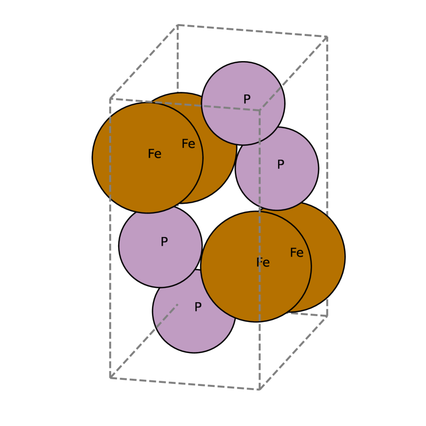
(a) Original

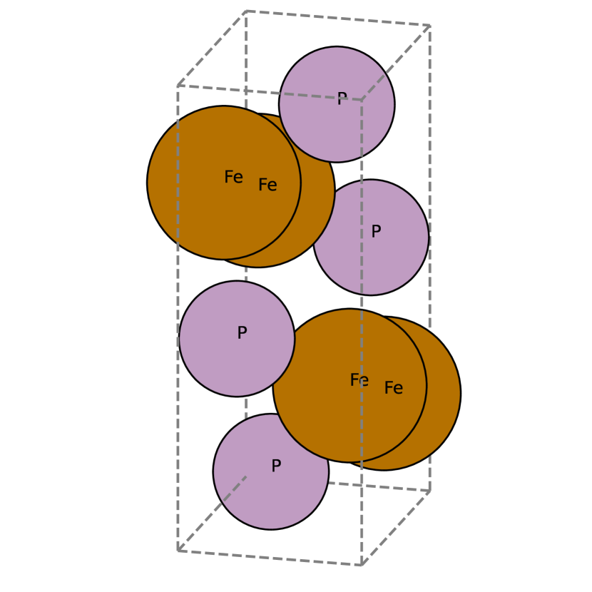
(b) Strain

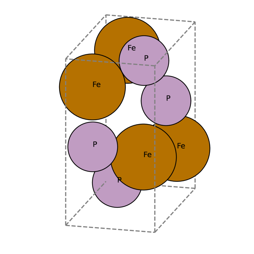
(c) Perturb

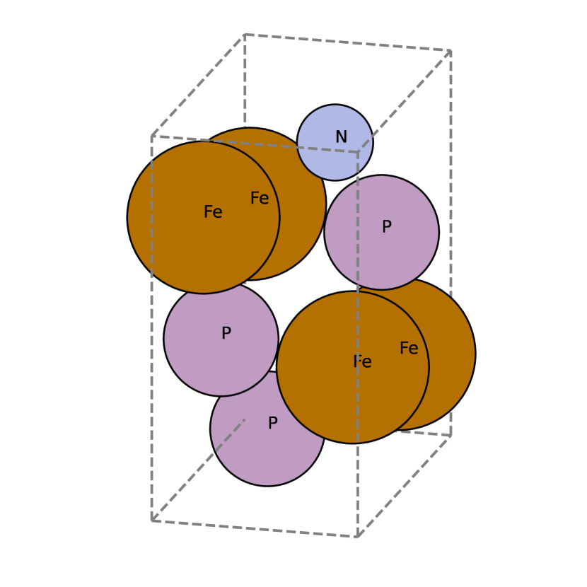
(d) Column replace

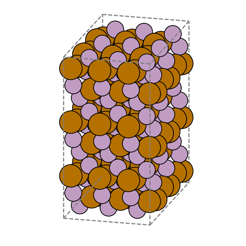
(e) Supercell

Figure 1: Visualizations of the crystal transformations used. All transforms are stochastic by nature with the exception of supercell.

We investigate four transformations specific to crystalline materials (Fig. 1). Each transformation is isoelectronic, preserving the valence electron configuration of the material: (1) perturb structure: each site is perturbed by a distance uniformly sampled between 0 and 50% of the minimum pairwise distance within the structure; (2) strain: a random, anisotropic tensile strain deformation is applied to the structure. Each lattice vector is increased by a factor uniformly sampled from $[0,0.05]$; (3) column replace: with probability $1$, a single, randomly selected site within the structure is replaced with an element from the same column in the periodic table as the original element; and (4) supercell: a supercell of the original crystal is created, scaling each lattice vector by a factor of $3$. The perturb structure strength range is selected based on values used in prior work [9], and the strain strength range is selected based on physically reasonable values.

2.2 Optimizing for composition similarity

Under the notion that materials with similar composition may tend to have similar properties, we hypothesize that explicitly guiding representations of similarly composed materials together may improve the representation quality. We propose an additional loss term, composition similarity (CS), to promote representation similarity among materials that have one or more common elements. Each crystal is assigned a binary vector $a\in\{0,1\}^{100}$, indicating which of the possible 100 atoms (that exist in the dataset used) are contained in the crystal. The set $P(i)=\{p\in I:a_{i}\cdot a_{p}>0,i\neq p\}$ is the set of indices that share one or more atom with the $i^{th}$ crystal. The loss can then be defined as:

$$\mathcal{L}^{\text{CS}}_{i}=-\log\Bigl{\{}\frac{1}{|P(i)|}\sum_{j\in P(i)}\frac{\exp(\text{sim}(z_{i},z_{j})/\tau)}{\sum^{2N}_{k=1}\mathbbm{1}_{[k\neq i]}\exp(\text{sim}(z_{i},z_{k})/\tau)}\Bigr{\}}$$ (2)

Where $|P(i)|$ is the cardinality of the set. While prior work in [15] has shown that placement of the summation over positives outside the $\log$ is more theoretically optimal, we found the above formulation to produce better representations empirically. In the final model, (2) is used in combination with the original NT-Xent loss (1) and weighted equally.

2.3 Learning Task Description

Our self-supervised training dataset consists of 90,160 crystal structures downloaded from Materials Project in April, 2021 [17]. For evaluation, we use additional melting temperature, thermal conductivity, and bulk moduli (K_VRH) datasets of sizes 3,014, 5,540, and 13,121 respectively. The melting temperature data were experimental data scraped from MatWeb [18]. Thermal conductivity data were downloaded from AFLOW [19]; all values are at 300K. Bulk moduli data were downloaded from Materials Project. Each dataset is split 80/10/10 into train, test, and validation sets.

3 Experimental Setup and Results

3.1 Augmentation Study

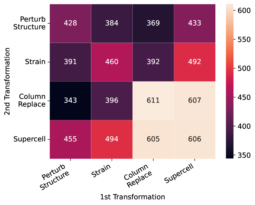
Figure 2: Linear regression evaluation of mean-absolute-error (MAE) of melting temperature. Single transformations are applied for elements along the diagonal, while other elements contain two transformations applied sequentially.

To evaluate the effects of individual and combinations of augmentations, we train models under all of the pairwise combinations of augmentations. For this study, we apply augmentations to only one sample in each positive pair. Each model is evaluated by performing a linear regression on the learned representations for each of the studied material properties. In our work, we use no augmentations for evaluation. Similar to [12, 13], we observe that the composition of transformations is crucial for representation quality. As shown in Figure 2 for melting point prediction, the best representations are obtained using the perturb-structure and column-replace transformations, and the addition of supercell often deteriorates performance. We observe a similar trend across all of the studied material properties.

3.2 Model Evaluation

We selected perturb-structure, strain, and column-replace as the final set of data augmentations; each augmentation has a 50% chance of being applied to each training sample. We trained two self-supervised models; each model was trained for 5000 epochs, with a batch size of $512$. The first model (CrystalCLR) uses $\mathcal{L}^{\text{CLR}}$ alone, while the second model (CrystalCLR+CS) uses a final loss of $\mathcal{L}^{\text{CLR}}+\mathcal{L}^{\text{CS}}$. We use the Adam optimizer [20] with a learning rate of 1e-4.

To quantitatively evaluate the learned representations, we trained random-forest regression models [21] to predict material properties. We compare the predictive performance of the learned embeddings to several other material fingerprinting methods, all obtainable without supervision: (1) Site stats fingerprint that aggregates statistics of the CrystalNNFingerprint [22] using structural order parameters, (2) Sine Coulomb fingerprint which is a variant of the Coloumb matrix for periodic crystals [23], and (3) Element property which is a weighted mean, standard deviation, minimum and maximum of element properties obtained from Magpie [24]. See Table 2 for the list of properties used. We use the default hyperparameters for the random forest from scikit-learn [25].

Table 1 shows the representations learned from contrastive training perform at or above traditional fingerprinting methods, with the exception of element properties. Element properties contain additional information, including melting point, which explain its high performance. Furthermore, we observe that the addition of the composition loss yields an improvement in performance across all properties.

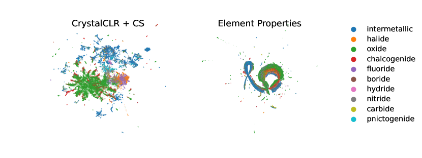
Figure 3: UMAP [26] visualizations of CrystalCLR + CS and Element Properties embeddings, colored by compound classes.

We also evaluate the use of contrastive learning as a pretraining task for material property prediction. For each of aforementioned properties, we train CGCNN models; one randomly initialized, and one initialized with the CGCNN encoder weights from each of the two contrastive training methods. For each model, we use the Adam optimizer [20] to fine-tune the models, using the learning rate with the best validation performance.

Table 1 shows by transferring weights from the contrastive-pretrained encoder, we are able to obtain more accurate predictions of material properties than a randomly initialized model for melting temperature and bulk moduli. The benefit of the composition loss is more evident for melting temperature prediction than the thermal conductivity and bulk moduli properties.

Lastly, in Figure 3 we visualize produced crystal embeddings using UMAP [26]. CrystalCLR learns representations that form clusters by compound class, despite training in a self-supervised manor.

	Melting temp (∘C)	Thermal cond. (Wm-1K-1)	K_VRH (GPa)
Random Forest evaluation:
Site Stats Fingerprint	$415.7\pm 2.2$	$5.41\pm 0.02$	$43.02\pm 0.11$
Sine Coulomb Fingerprint	$336.7\pm 2.2$	$3.50\pm 0.03$	$25.74\pm 0.13$
Element Properties	$\textbf{106.1}\pm 1.6$	$\textbf{3.39}\pm 0.03$	$\textbf{17.64}\pm 0.07$
CrystalCLR (ours)	$161.7\pm 2.5$	$3.73\pm 0.03$	$21.98\pm{0.11}$
CrystalCLR + CS (ours)	$156.7\pm 1.8$	$3.51\pm 0.03$	$20.79\pm 0.07$
Fine-tune:
Random init	$119.9\pm 2.0$	$3.08\pm 0.16$	$13.13\pm 0.25$
CrystalCLR (ours)	$106.8\pm 6.0$	$\textbf{3.04}\pm 0.33$	$\textbf{12.89}\pm 0.19$
CrystalCLR + CS (ours)	$\textbf{102.8}\pm 2.6$	$3.11\pm 0.13$	$12.95\pm 0.28$

Table 1: Evaluation of models, measured in mean absolute error. Each reported value is the mean over five random seeds, along with standard deviation

4 Conclusion

In this work, we introduce a method for the contrastive training of graph neural networks for representation learning of materials. First, we establish several crystalline material specific transformations, and study the effects of the composition of transformations on representation quality. In addition, we introduce a novel loss function to explicitly maximize the similarity among materials that share common elements. We show that our framework is capable of producing representations competitive with engineered material fingerprinting techniques. Finally we show that constrastive pretraining improves performance over random initialization for downstream tasks. Future work will investigate additional contrastive learning methods, the ability to use CrystalCLR representations for material retrieval, and the applicability of equivariant graph neural networks.

5 Appendix

5.1 Element Properties List

Table 2 lists the element properties used for the Element Property classifier.

Feature Name	Description
Number	Atomic Number
MendeleevNumber	Mendeleev Number (position on the periodic table, counting columnwise from H)
AtomicWeight	Atomic weight
MeltingT	Melting temperature of element
Column	Column on periodic table
Row	Row on periodic table
CovalentRadius	Covalent radius of each element
Electronegativity	Pauling electronegativity
NsValence	Number of filled s valence orbitals
NpValence	Number of filled p valence orbitals
NdValence	Number of filled d valence orbitals
NfValence	Number of filled f valence orbitals
NValence	Number of valence electrons
NsUnfilled	Number of unfilled s valence orbitals
NpUnfilled	Number of unfilled p valence orbitals
NdUnfilled	Number of unfilled d valence orbitals
NfUnfilled	Number of unfilled f valence orbitals
NUnfilled	Number of unfilled valence orbitals
GSvolume_pa	DFT volume per atom of T=0K ground state
GSbandgap	DFT bandgap energy of T=0K ground state
GSmagmom	DFT magnetic moment of T=0K ground state
SpaceGroupNumber	Space group of T=0K ground state structure

Table 2: Element properties used. Feature names and descriptions are reproduced from the supplementary materials of Ward et al. [24].

References

- Schleder et al. [2019] Gabriel R. Schleder, Antonio C. M. Padilha, Carlos Mera Acosta, Marcio Costa, and Adalberto Fazzio. From dft to machine learning: recent approaches to materials science–a review. Journal of Physics: Materials, 2(3):032001, 2019.
- Ramprasad et al. [2017] Rampi Ramprasad, Rohit Batra, Ghanshyam Pilania, Arun Mannodi-Kanakkithodi, and Chiho Kim. Machine learning in materials informatics: recent applications and prospects. npj Computational Materials, 3(54), 2017.
- Xie and Grossman [2018] Tian Xie and Jeffrey C Grossman. Crystal graph convolutional neural networks for an accurate and interpretable prediction of material properties. Physical review letters, 120(14):145301, 2018.
- Chen et al. [2019] Chi Chen, Weike Ye, Yunxing Zuo, Chen Zheng, and Shyue Ping Ong. Graph networks as a universal machine learning framework for molecules and crystals. Chemistry of Materials, 31(9):3564–3572, 2019. doi: 10.1021/acs.chemmater.9b01294. URL https://doi.org/10.1021/acs.chemmater.9b01294.
- Louis et al. [2020] Steph-Yves Louis, Yong Zhao, Alireza Nasiri, Xiran Wang, Yuqi Song, Fei Liu, and Jianjun Hu. Graph convolutional neural networks with global attention for improved materials property prediction. Physical Chemistry Chemical Physics, 22(32):18141–18148, 2020. ISSN 1463-9084. doi: 10.1039/d0cp01474e. URL http://dx.doi.org/10.1039/D0CP01474E.
- Griggs et al. [2020] Petar Griggs, Lin Li, and Rajmonda Caceres. Unified gnn architecture design for high-throughput material screening. 2020.
- Batzner et al. [2022] Simon Batzner, Albert Musaelian, Lixin Sun, Mario Geiger, Jonathan P Mailoa, Mordechai Kornbluth, Nicola Molinari, Tess E Smidt, and Boris Kozinsky. E (3)-equivariant graph neural networks for data-efficient and accurate interatomic potentials. Nature communications, 13(1):1–11, 2022.
- Musaelian et al. [2022] Albert Musaelian, Simon Batzner, Anders Johansson, Lixin Sun, Cameron J Owen, Mordechai Kornbluth, and Boris Kozinsky. Learning local equivariant representations for large-scale atomistic dynamics. arXiv preprint arXiv:2204.05249, 2022.
- Magar et al. [2021] Rishikesh Magar, Yuyang Wang, Cooper Lorsung, Chen Liang, Hariharan Ramasubramanian, Peiyuan Li, and Amir Barati Farimani. Auglichem: Data augmentation library ofchemical structures for machine learning, 2021.
- Fung et al. [2021] Victor Fung, Jiaxin Zhang, Eric Juarez, and Bobby G Sumpter. Benchmarking graph neural networks for materials chemistry. npj Computational Materials, 7(1):1–8, 2021.
- Lee and Asahi [2021] Joohwi Lee and Ryoji Asahi. Transfer learning for materials informatics using crystal graph convolutional neural network. Computational Materials Science, 190:110314, 2021.
- Chen et al. [2020] Ting Chen, Simon Kornblith, Mohammad Norouzi, and Geoffrey Hinton. A simple framework for contrastive learning of visual representations. In International conference on machine learning, pages 1597–1607. PMLR, 2020.
- You et al. [2020] Yuning You, Tianlong Chen, Yongduo Sui, Ting Chen, Zhangyang Wang, and Yang Shen. Graph contrastive learning with augmentations. Advances in Neural Information Processing Systems, 33:5812–5823, 2020.
- Wang et al. [2022] Yuyang Wang, Jianren Wang, Zhonglin Cao, and Amir Barati Farimani. Molecular contrastive learning of representations via graph neural networks. Nature Machine Intelligence, 4(3):279–287, 2022.
- Khosla et al. [2020] Prannay Khosla, Piotr Teterwak, Chen Wang, Aaron Sarna, Yonglong Tian, Phillip Isola, Aaron Maschinot, Ce Liu, and Dilip Krishnan. Supervised contrastive learning. Advances in Neural Information Processing Systems, 33:18661–18673, 2020.
- Sohn [2016] Kihyuk Sohn. Improved deep metric learning with multi-class n-pair loss objective. Advances in neural information processing systems, 29, 2016.
- Jain et al. [2013] Anubhav Jain, Shyue Ping Ong, Geoffroy Hautier, Wei Chen, William Davidson Richards, Stephen Dacek, Shreyas Cholia, Dan Gunter, David Skinner, Gerbrand Ceder, et al. Commentary: The materials project: A materials genome approach to accelerating materials innovation. APL materials, 1(1):011002, 2013.
- Gao et al. [2013] Zhi-Yu Gao, Guo-Quan Liu, et al. Recent progress of web-enable material database and a case study of nims and matweb. Journal of Materials Engineering, 3(11):89–96, 2013.
- Curtarolo et al. [2012] Stefano Curtarolo, Wahyu Setyawan, Shidong Wang, Junkai Xue, Kesong Yang, Richard H. Taylor, Lance J. Nelson, Gus L.W. Hart, Stefano Sanvito, Marco Buongiorno-Nardelli, Natalio Mingo, and Ohad Levy. Aflowlib.org: A distributed materials properties repository from high-throughput ab initio calculations. Computational Materials Science, 58:227–235, 2012. ISSN 0927-0256. doi: https://doi.org/10.1016/j.commatsci.2012.02.002. URL https://www.sciencedirect.com/science/article/pii/S0927025612000687.
- Kingma and Ba [2014] Diederik P Kingma and Jimmy Ba. Adam: A method for stochastic optimization. arXiv preprint arXiv:1412.6980, 2014.
- Breiman [2001] Leo Breiman. Random forests. Machine learning, 45(1):5–32, 2001.
- Zimmermann and Jain [2020] Nils ER Zimmermann and Anubhav Jain. Local structure order parameters and site fingerprints for quantification of coordination environment and crystal structure similarity. RSC advances, 10(10):6063–6081, 2020.
- Faber et al. [2015] Felix Faber, Alexander Lindmaa, O Anatole von Lilienfeld, and Rickard Armiento. Crystal structure representations for machine learning models of formation energies. International Journal of Quantum Chemistry, 115(16):1094–1101, 2015.
- Ward et al. [2016] Logan Ward, Ankit Agrawal, Alok Choudhary, and Christopher Wolverton. A general-purpose machine learning framework for predicting properties of inorganic materials. npj Computational Materials, 2(1):1–7, 2016.
- Pedregosa et al. [2011] F. Pedregosa, G. Varoquaux, A. Gramfort, V. Michel, B. Thirion, O. Grisel, M. Blondel, P. Prettenhofer, R. Weiss, V. Dubourg, J. Vanderplas, A. Passos, D. Cournapeau, M. Brucher, M. Perrot, and E. Duchesnay. Scikit-learn: Machine learning in Python. Journal of Machine Learning Research, 12:2825–2830, 2011.
- McInnes et al. [2018] Leland McInnes, John Healy, and James Melville. Umap: Uniform manifold approximation and projection for dimension reduction. arXiv preprint arXiv:1802.03426, 2018.