Differentially Private Image Classification from Features

Abstract

In deep learning, leveraging transfer learning has recently been shown to be an effective strategy for training large high performance models with Differential Privacy (DP). Moreover, somewhat surprisingly, recent works have found that privately training just the last layer of a pre-trained model provides the best utility with DP. While past studies largely rely on using first-order differentially private training algorithms like DP-SGD for training large models, in the specific case of privately learning from features, we observe that computational burden is often low enough to allow for more sophisticated optimization schemes, including second-order methods. To that end, we systematically explore the effect of design parameters such as loss function and optimization algorithm. We find that, while commonly used logistic regression performs better than linear regression in the non-private setting, the situation is reversed in the private setting. We find that least-squares linear regression is much more effective than logistic regression from both privacy and computational standpoint, especially at stricter epsilon values ($\varepsilon<1$). On the optimization side, we also explore using Newton’s method, and find that second-order information is quite helpful even with privacy, although the benefit significantly diminishes with stricter privacy guarantees. While both methods use second-order information, least squares is more effective at lower epsilon values while Newton’s method is more effective at larger epsilon values. To combine the benefits of both methods, we propose a novel optimization algorithm called DP-FC, which leverages feature covariance instead of the Hessian of the logistic regression loss and performs well across all $\varepsilon$ values we tried. With this, we obtain new SOTA results on ImageNet-1k, CIFAR-100 and CIFAR-10 across all values of $\varepsilon$ typically considered. Most remarkably, on ImageNet-1K, we obtain top-1 accuracy of 88% under DP guarantee of (8, $8*10^{-7}$) and 84.3% under (0.1, $8*10^{-7}$).

1 Introduction

Despite impressive performance, large machine learning models are susceptible to attacks. Previous work has demonstrated successful membership attacks where the goal is to extract exact instances of training examples that the model was trained on (Shokri et al., 2017; Carlini et al., 2019, 2021; Choquette-Choo et al., 2020; Liu et al., 2021b; Balle et al., 2022) and models of larger size are known to be more likely to memorize training data. These attacks can be quite egregious if the model was trained on sensitive data like personal photos or emails. One approach to mitigate this risk is to train such models with privacy guarantees. In particular, Differential Privacy (DP) has become the gold standard in quantifying the risk and providing formal guarantees against membership attacks (Nasr et al., 2021).

Informally, Differentially Privacy implies that an adversary learns almost the same thing about an individual data point independent of their presence or absence in the training data set. More formally, DP is defined as follows:

Definition 1.1 (Differential Privacy (Dwork et al., 2006b, a)).

A randomized algorithm $\mathcal{A}$ is $(\varepsilon,\delta)$-differentially private if, for any pair of datasets $D$ and $D^{\prime}$ differing in at most one example (called neighboring datasets), and for all events $\mathcal{S}$ in the output range of $\mathcal{A}$, we have

$$\mathop{\mathbf{Pr}}[\mathcal{A}(D)\in\mathcal{S}]\leq e^{\varepsilon}\cdot\mathop{\mathbf{Pr}}[\mathcal{A}(D^{\prime})\in\mathcal{S}]+\delta,$$

where the probability is over the randomness of $\mathcal{A}$.

In the field of deep learning, Differentially Private Stochastic Gradient Descent (DP-SGD) (Song et al., 2013; Bassily et al., 2014; Abadi et al., 2016) is the most commonly used method for training models with DP guarantees. While DP-SGD is a fairly general algorithm, a naive application can suffer from several computational challenges. To make matters worse, the gap between performance of a model with and without privacy typically widens as the model is made larger. This stands as a significant obstacle to a wider adoption and deployment of large practical models with privacy guarantees.

For the problem of Image Classification, several works have shown that transfer learning can be a very effective strategy in order to improve privacy-utility trade-off when formal privacy guarantees are required (Kurakin et al., 2022; Mehta et al., 2022; De et al., 2022). In this setting, a model is first pre-trained with “non-sensitive” data without privacy guarantees, then fine-tuned on a “sensitive” dataset over which a formal privacy guarantee is required. Similar to previous works, we simulate several publicly available image classification benchmarks (like ImageNet) as “sensitive” datasets.

Interestingly, Mehta et al. (2022); De et al. (2022) observe that privately fine-tuning just the last layer of a pre-trained model (using DP-SGD) leads to state of the art results in the ImageNet-1k dataset. This is quite fortuitous, since privately fine-tuning the full model typically introduces significant computational challenges. We build on this observation, and perform a comprehensive exploration of various design parameters, including the choice of loss function and optimization algorithm, beyond simple DP-SGD. In this restricted setting of learning a single layer privately using features extracted from a pre-trained model, more sophisticated methods, such as second-order methods, are computationally viable. Our main contributions are as follows:

• Somewhat surprisingly, we find that linear regression solved using DP Least Squares performs much better than logistic regression solved using DP-SGD, especially at lower epsilons.

• Postulating that the benefits largely stem from the use of second-order information in the least squares solution, we further explore using Newton’s method to solve logistic regression. While Newton’s method outperforms linear regression in the non-private setting, we find that it still performs worse with privacy constraints, largely because sanitizing the Hessian with logistic regression requires adding far more noise than in linear regression, where part of the Hessian can be shared across all classes.

• To combine the benefits of both, we introduce a method which we call Differentially Private SGD with Feature Covariance (abbreviated as DP-FC) where we simply replace the Hessian in Newton’s method with sanitized Feature Covariance. Using Feature Covariance instead of Hessian allows us to make use of second-order information in the training procedure while sharing it across classes and iterations, which greatly reduces the amount of noise that needs be added to sanitize it. This allows us to continue using logistic regression, which performs better in non-private setting, while benefiting from improved privacy-utility trade-off as seen with linear regression in the private setting.

• With DP-FC, we surpass previous state of the art results considerably on 3 image classification benchmarks, namely ImageNet-1k, CIFAR-10 and CIFAR-100, just by performing DP fine-tuning on features extracted from a pre-trained model, see Table 1 for a summary. Consistent with previous works, we also find that performance increases as the pre-training dataset and the model are made larger.

Dataset	Epsilon	Previous SOTA	Accuracy	Method	Epochs ($=$ Steps)	Pretraining DS
CIFAR-10	0.01		97.4	DP-LS	1	JFT
	0.05		98.2	DP-FC	10	JFT
	0.1		98.4	DP-FC	10	JFT
	0.5		98.8	DP-FC	10	JFT
	1.0	96.7	98.8	DP-FC	10	JFT
	2.0	97.1	98.9	DP-FC	10	JFT
	4.0	97.2	98.9	DP-FC	10	JFT
	8.0	97.4	98.9	DP-FC	10	JFT
	$\infty$		98.9	LS	1	JFT
CIFAR-100	0.01		77.2	DP-LS	1	I21K
	0.05		80.3	DP-LS	1	JFT
	0.1		82.5	DP-LS	1	JFT
	0.5		86.2	DP-FC	10	JFT
	1.0	83.0	88.1	DP-FC	10	JFT
	2.0	86.2	89.0	DP-FC	10	JFT
	4.0	87.7	90.0	DP-FC	10	JFT
	8.0	88.4	90.1	DP-FC	10	JFT
	$\infty$		90.6	LS	1	JFT
ImageNet-1K	0.01		82.4	DP-LS	1	JFT
	0.05		83.8	DP-LS	1	JFT
	0.1		84.3	DP-FC	1	JFT
	0.5		86.1	DP-FC	10	JFT
	1.0	84.4	86.8	DP-FC	10	JFT
	2.0	85.6	87.4	DP-FC	10	JFT
	4.0	86.0	87.7	DP-FC	10	JFT
	8.0	86.7	88.0	DP-FC	10	JFT
	$\infty$		88.9	Newton	10	JFT

Table 1: Compilation of our best private Top-1 test accuracies. All number are SOTA across all epsilons to the best of our knowledge. Previous state of the art for CIFAR-10 and CIFAR-100 were reported form Bu et al. (2022a) and for ImageNet-1K from De et al. (2022). We denote $\varepsilon$ to be $\infty$ for non-private setting where we turn off all sanitization steps including clipping. We set $\delta$ to $8*10^{-7}$ for ImageNet-1k, and $1*10^{-5}$ for CIFAR-10 and CIFAR-100. Interestingly, in the non-private setting, most previous works (including Zhai et al. (2021)) use Linear Regression when finetuning from features but we found that Logistic Regression (solved using Newton’s method) performs much better and leads to an impressive 88.9% accuracy when finetuning just the last layer. To put this in perspective, this is only 1.1% less than the current state of the art non-private accuracy of 91% on ImageNet-1k (Yu et al., 2022b). We report extensive hyperparameter details in the appendix for reproducibility of our results.

2 Private Learning from Features

In this section, we describe the details of optimization strategies we considered, and state the privacy guarantees for each of them.

Given a data set $\mathcal{D}=\{(x_{1},y_{1}),\cdots,(x_{n},y_{n})\}$, we optimize the function $\mathcal{L}:\mathbb{R}^{m\times d}\to\mathbb{R}$ defined as follows

$$\mathcal{L}(\theta)\triangleq\frac{1}{n}\sum_{i=1}^{n}\sum_{j=1}^{m}\ell(\langle\theta_{j},x_{i}\rangle,y_{ij})$$ (1)

where $n$ is the number of examples, $m$ is the number of classes, $\theta\in\mathbb{R}^{m\times d}$ is the weight matrix to be learned, $x_{i}$ is the feature vector for example $i$, $y_{ij}$ is the label of example $i$ and class $j$, and $\ell$ is a convex loss function. We assume that $y_{ij}\in[0,1]$ for all $i,j$. Additionally, we also use the short hand $\ell(\theta;(x_{i},y_{i}))=\sum_{j=1}^{m}\ell(\langle\theta_{j},x_{i}\rangle,y_{ij})$ where helpful in order to simplify the notation.

In the case of learning from features extracted from a pre-trained model, the feature vectors $x_{i}$ are last layer features. Further, unless otherwise specified, we will assume $\ell$ to be the logistic loss, i.e. $\ell_{\text{logistic}}(z,y)=-y\log\sigma(z)-(1-y)\log(1-\sigma(z))$ where $\sigma(z)=\frac{1}{1+e^{-z}}$. Finally, we will also assume that each step of optimization considers the whole batch, which greatly simplifies both the privacy analysis of algorithms and the experiments. Rest of this section includes descriptions of several iterative solvers of this minimization problem, both in non-private and private settings. Some of these methods rely on the fact that we are only interested in fine-tuning just the last layer, while others are more general. In the privacy analysis, we use zCDP (zero - Concentrated Differential Privacy) Bun and Steinke (2016), but we state our empirical results always with final privacy guarantee in $(\varepsilon,\delta)$-DP terms, as done in previous works.

2.1 DP-SGD

Arguably the most popular approach to solving the above minimization problem in the non-private setting is Stochastic Gradient Descent (SGD). In the full-batch setting, at every iteration, SGD performs the update:

$$g_{t}\leftarrow\frac{1}{n}\sum_{i=1}^{n}\nabla\ell(\theta_{t};(x_{i},y_{i}))\qquad\theta_{t+1}=\theta_{t}-\eta_{t}g_{t}$$ (2)

where $\eta_{t}$ denotes the learning rate used for for iteration $t$.

DP-SGD is a private variant of this algorithm and the baseline in all our experiments. Computationally, in order to bound the sensitivity of each training example, Abadi et al. (2016) suggest computing a gradient for each example separately and clipping each to a maximum norm of $C$ (a user-specified hyper-parameter):

$$g_{t}\leftarrow\sum_{i=1}^{n}{\sf clip}\left(\nabla\ell(\theta_{t};(x_{i},y_{i}))\right)\qquad\tilde{g}_{t}\leftarrow\frac{g_{t}+\mathcal{N}\left(0,(\sigma C)^{2}\right)}{n}$$ (3)

where ${\sf clip}(v)=v\cdot\min\left\{1,\frac{C}{\|v\|_{2}}\right\}$.

After summing the clipped example gradients, a noise vector sampled from a Gaussian distribution with standard deviation $\sigma C$ is added, where $\sigma$ is a parameter that determines the privacy guarantee via the Gaussian mechanism.

As shown in Algorithm 1, once the gradient has been sanitized, we are free to use it to accumulate statistics (e.g. first or second moment estimates) which are typically useful with the optimization process. Algorithm 1 presents a generalized version of DP-SGD where the gradients get processed in the traditional DP-SGD fashion, and are then passed to a first-order optimizer as an input. This lets us instantiate DP versions of well-known first-order optimizers like SGD, Momentum and Adam. We employ DP-Adam in all our experiments. Finally, we omit the privacy analysis for the DP-SGD baseline since it is standard, but we do include in the appendix the details of the implementation we used for translation from privacy constraints to noise scale.

Algorithm 1 Generalized First Order Differentially Private Algorithm

0:  Data set $D=\{(x_{1},y_{1}),\cdots,(x_{n},y_{n})\}$ with $(x_{i},y_{i})\in\mathcal{D}$, loss function: $\ell:\mathbb{R}^{m\times d}\times\mathbb{R}\to\mathbb{R}$, a first order optimizer $Opt$, clipping norm: $C$, number of iterations: $T$, noise multiplier: $\sigma$

1:  Randomly initialize $\theta_{0}$.

2:  for $t=1,\dots,T$ do

3:     $g_{t}\leftarrow\frac{1}{n}\sum_{i=1}^{n}{\sf clip}\left(\nabla\ell(\theta_{t};(x_{i},y_{i}))\right)$, where ${\sf clip}(v)=v\cdot\min\left\{1,\frac{C}{\|v\|_{2}}\right\}$.

4:     $\tilde{g_{t}}\leftarrow g_{t}+\mathcal{N}\left(0,(\sigma C)^{2}\right)$

5:     $\theta_{t+1}\leftarrow$ single step of first order optimization with gradient $Opt(\tilde{g_{t}})$

6:  end for

7:  return $\frac{1}{T}\sum\limits_{t=1}^{T}\theta_{t}$ or $\theta_{T}$.

2.2 DP-Newton

Since the optimization problem under consideration is a relatively simple convex problem, second-order DP algorithms can be viable. We first consider a privatized version of the popular Newton’s method and denote it as DP-Newton. To control the sensitivity of each training example, one naive approach is to compute per-example Hessians and clip their norm, in a similar fashion to example gradient clipping in DP-SGD. But even in our last-layer fine-tuning setting, this can be prohibitively expensive. For instance, training on features extracted from ViT-G for ImageNet-1k fine-tuning, Hessian tensor (in a block diagonal form) is of size [1000, 1664, 1664] with approximately 2.8B entries. In order to avoid instantiating the Hessian for every training example, we instead choose to clip the feature vectors $x_{i}$, then translate the clipping threshold into bounds on the Hessian and gradient norms. This is summarized in Algorithm 2.

Algorithm 2 Differentially Private Newton’s Method

0:  Data set $D=\{(x_{1},y_{1}),\cdots,(x_{n},y_{n})\}$ with $(x_{i},y_{i})\in\mathcal{D}$, loss function: $\ell:\mathbb{R}^{d}\times\mathbb{R}\to\mathbb{R}$, regularization coefficient $\lambda$, learning rate $\eta$, clipping norm: $C$, number of iterations: $T$, noise multiplier: $\sigma$, bound on the second derivative of the loss: $\beta_{H}$

1:  Clip all features: $\tilde{x}_{i}\leftarrow{\sf clip}(x_{i})$ for all $i\in\{1,\dots,n\}$ where ${\sf clip}(v)=v\cdot\min\left\{1,\frac{C}{\|v\|_{2}}\right\}$.

2:  Randomly initialize $\theta_{0}$.

3:  for $t=1,\dots,T$ do

4:     for $j=1,\dots,m$ do

5:        $g_{t,j}\leftarrow\sum_{i=1}^{n}\nabla\ell(\theta_{t,j}^{\top}\tilde{x}_{i},y_{ij})$.

6:        $H_{t,j}\leftarrow\sum_{i=1}^{n}\nabla^{2}\ell(\theta_{t,j}^{\top}\tilde{x}_{i},y_{ij})+\lambda I$

7:        $\tilde{g}_{t,j}\leftarrow\frac{1}{n}g_{t,j}+\mathcal{N}\left(\vec{0}_{d},(\frac{\sigma C\sqrt{m}}{n})^{2}\right)$ where $\mathcal{N}\left(\vec{0}_{d},(\frac{\sigma C\sqrt{m}}{n})^{2}\right)$ indicates a $d$-dimensional vector each of whose coordinates is an i.i.d. Gaussian with standard deviation $\sigma C\sqrt{m}/n$.

8:        $\tilde{H}_{t,j}\leftarrow\frac{1}{n}H_{t,j}+\mathcal{N}\left(\vec{0}_{d\times d},\left(\frac{\sigma\beta_{H}C^{2}\sqrt{m}}{n}\right)^{2}\right)$ where $\mathcal{N}\left(\vec{0}_{d\times d},\left(\frac{\sigma\beta_{H}C^{2}\sqrt{m}}{n}\right)^{2}\right)$ indicates a $d\times d$ matrix each of whose coordinates is an i.i.d. Gaussian with standard deviation $\sigma\beta_{H}C^{2}\sqrt{m}/n$.

9:        $\theta_{t+1,j}\leftarrow\theta_{t,j}-\eta{\tilde{H}_{t,j}}^{-1}\tilde{g}_{t,j}$

10:     end for

11:  end for

12:  return $\theta_{T}$.

Theorem 2.1 (Privacy guarantee for Algorithm 2).

Suppose $\ell$ is twice differentiable, and that for all $(z,y)$, $|\ell^{\prime}(z,y)|\leq 1$ and $|\ell^{\prime\prime}(z,y)|\leq\beta_{H}$. Then, Algorithm 2 satisfies $\frac{T}{\sigma^{2}}$-zCDP.

Here $\ell^{\prime}$ and $\ell^{\prime\prime}$ denote the first and second derivatives of $\ell$ with respect to its first argument. We choose the bound on the first derivative to be $1$ without loss of generality (via scaling of $\ell$). Note that the assumptions of the theorem are satisfied for the squared loss $\ell(z,y)=\frac{1}{2}(z-y)^{2}$ with $\beta_{H}=1$, as well as for the sigmoid cross-entropy loss (i.e. logistic regression) with $\beta_{H}=\frac{1}{4}$. Indeed, $|\ell_{\text{logistic}}^{\prime}(z,y)|=|y-\sigma(z)|$, and $|\ell_{\text{logistic}}^{\prime\prime}(z,y)|=\sigma(z)*(1-\sigma(z))$ where $\sigma(z)=\frac{1}{1+e^{-z}}$. The first expression is bounded by $1$ (since $y,\sigma(z)\in[0,1]$) and the second expression is bounded by $\frac{1}{4}$.

Proof.

The crux of the proof is to ensure that Lines 7 and 8 individually satisfy $\frac{1}{2m\sigma^{2}}$-zCDP. The rest of the proof is just simple composition of zCDP Bun and Steinke (2016) across $m$ classes and $T$ iterations. To see this, first let $D$ and $D^{\prime}$ be neighboring datasets and let $(x,y)$ be the differing datapoint between $D$ and $D^{\prime}$.

Now, notice that in the computation of $g_{t}$, we have the following: $\|g_{t,j}(D)-g_{t,j}(D^{\prime})\|=\|\ell^{\prime}(\langle\theta_{t,j},\tilde{x}\rangle,y_{j})\tilde{x}\|$. Thus, since $\left\|\tilde{x}\right\|_{2}\leq C$, and $|\ell^{\prime}(\langle\theta_{j},x\rangle,y_{j})|\leq 1$:

$$\left\|g_{t,j}(D)-g_{t,j}(D^{\prime})\right\|_{2}\leq{C}$$ (4)

From (4) it immediately follows that the computation of $g_{t,j}$ for each $t\in\{0,\ldots,T-1\}$ and each $j\in\{1,\dots,m\}$ satisfies $\frac{1}{2m\sigma^{2}}$-zCDP. Now, moving on to the sensitivity of $H_{t}$ in Line 8, we have $H_{t,j}(D)-H_{t,j}(D^{\prime})=\ell^{\prime\prime}(\langle\theta_{j},\tilde{x}\rangle,y_{j})\tilde{x}\tilde{x}^{\top}$. Then, since $\left\|\tilde{x}\right\|_{2}\leq C$ and $|\ell^{\prime\prime}(\langle\theta_{j},x\rangle,y_{j})|\leq\beta_{H}$, we have:

$$\left\|H_{t,j}(D)-H_{t,j}(D^{\prime})\right\|_{F}\leq\beta_{H}C^{2},$$ (5)

and (5) immediately implies that the computation of $H_{t,j}$ for each $t\in\{0,\ldots,T-1\}$ and $j\in\{1,\dots,m\}$ satisfies $\frac{1}{2m\sigma^{2}}$-zCDP. This completes the proof. ∎

2.3 DP-LS

One drawback of DP-SGD and DP-Newton is that each training example $i$ contributes to the gradients (resp. Hessians) of all classes $j\in\{1,\dots,m\}$, so the sensitivity (and hence the scale of required noise) increases with the number of classes. This is visible in Algorithm 2 where the amount of noise added for privacy protection scales with $\sqrt{m}$ (Lines 7 and 8). When the number of classes is large, this reduces signal-to-noise ratio and can hurt quality. In this section, we develop a method that aims to address this issue. We take inspiration from the matrix factorization literature, in which one can separate the loss function into the contribution of positive and negative classes. We assume that labels are binary ($y_{ij}\in\{0,1\}$), and we consider the following quadratic loss function:

$$\mathcal{L}(\theta)=\frac{1}{2}\sum_{i=1}^{n}\sum_{j=1}^{m}y_{ij}(x_{i}^{\top}\theta_{j}-y_{ij})^{2}+\frac{\alpha}{2}(x_{i}^{\top}\theta_{j})^{2}+\frac{\lambda}{2}\|\theta_{j}\|^{2},$$

in other words, we take $\ell(z,y)=\frac{1}{2}(y(z-y)^{2}+\alpha z^{2})$. The first term fits the positive labels (notice that this term vanishes when $y=0$), while the second term fits negative labels, and $\alpha$ is hyper-parameter that trades-off the two terms. This formulation was studied by Hu et al. (2008) and enjoys remarkable empirical success Koren and Bell (2015). It turns out that this method is also well-suited for privacy, as we shall discuss below.

By expanding the quadratic terms, we can write the loss as

$$\mathcal{L}(\theta) =\frac{1}{2}\sum_{j=1}^{m}\left(\theta_{j}^{\top}A_{j}\theta_{j}-2\theta_{j}^{\top}b_{j}+\alpha\theta_{j}^{\top}G\theta_{j}+\lambda\theta_{j}^{\top}\theta_{j}\right)$$

where for all $j\in\{1,\dots,m\}$

$$A_{j}=\sum_{i:y_{ij}=1}x_{i}x_{i}^{\top},\quad b_{j}=\sum_{i:y_{ij}=1}x_{i},\quad G=\sum_{i=1}^{n}x_{i}x_{i}^{\top}$$ (6)

The exact solution is then given by

$$\theta_{j}=\left[A_{j}+\alpha G+\lambda I\right]^{-1}b_{j}.$$

Notice that the solution $\theta_{j}$ for class $j$ depends on class-specific statistics (the matrix $A_{j}$ and the vector $b_{j}$), as well as the global quantity $G$. Algorithm 3 computes a private estimate of the solution by adding Gaussian noise to each of $G,A_{j},b_{j}$ (Lines 2, 4, and 5 respectively), then solving the linear system using the noised statistics (Line 6). This is a variant of the popular sufficient statistics perturbation algorithm for DP linear regression. One crucial observation is that the noisy version of $G$ is only computed once (Line 2), and reused for all classes. This allows to control the sensitivity of the solution w.r.t. each example; indeed, suppose example $i$ only has one positive class $j_{0}$, then that example only contributes to $G$, $A_{j_{0}}$, and $b_{j_{0}}$. In particular, the sensitivity of the solution (and hence the amount of noise we need to add) does not scale with the total number of classes, only with the number of positive classes per example. This is represented by the parameter $k$ in Algorithm 3 ($k$ is equal to $1$ for single-class classification tasks, and even in multi-class tasks, we typically have $k\ll m$). We now give the formal privacy guarantee:

Theorem 2.2 (Privacy guarantee for Algorithm 3).

Algorithm 3 satisfies $\frac{3}{2\sigma^{2}}$-zCDP.

Proof.

First, let $D,D^{\prime}$ be neighboring data sets that differ in the data point $(x,y)$, and let $G(D)$ be the global statistic in (6) computed on data set $D$. Then $\|G(D)-G(D^{\prime})\|_{F}=\|\tilde{x}\tilde{x}^{\top}\|_{2}$, and since $\|\tilde{x}\|_{2}\leq C$ (due to clipping), $\|G(D)-G(D^{\prime})\|_{F}\leq C^{2}$, thus the computation of $G$ (Line 2) is $\frac{1}{2\sigma^{2}}$-zCDP. Now moving to the computation of $A_{j}$: let $A(D)$ be the concatenation of all the class-specific statistics, i.e. $A(D)=[A_{1}(D)|\dots|A_{m}(D)]$. Notice that $\|A_{j}(D)-A_{j}(D^{\prime})\|_{F}=\|\tilde{x}\tilde{x}^{\top}\|_{2}$ if $y_{j}=1$ and $0$ otherwise. Since by assumption, the number of positive classes per example is bounded by $k$, we have that $\|A(D)-A(D^{\prime})\|_{F}\leq\sqrt{k}\|\tilde{x}\tilde{x}^{\top}\|_{F}$, which is bounded by $\sqrt{k}C^{2}$ due to clipping. Therefore the computation of all $A_{j}$ combined (Line 4) is $\frac{1}{2\sigma^{2}}$-zCDP. Finally, by a similar argument, we have that $\|b(D)-b(D^{\prime})\|_{2}\leq\sqrt{k}C$, and the computation of all $b_{j}$ combined (Line 5) is $\frac{1}{2\sigma^{2}}$-zCDP.

By simple composition of zCDP Bun and Steinke (2016), the algorithm is $\frac{3}{2\sigma^{2}}$-zCDP. ∎

Algorithm 3 Differentially Private Least Squares

0:  Data set $D=\{(x_{1},y_{1}),\cdots,(x_{n},y_{n})\}$ with $(x_{i},y_{i})\in\mathcal{D}$, weight coefficient $\alpha$, regularization coefficient $\lambda$, maximum number of positive classes per example: $k$, clipping norm: $C$, noise multiplier: $\sigma$.

1:  Clip all features: $\tilde{x}_{i}\leftarrow{\sf clip}(x_{i})$ for all $i\in\{1,\dots,n\}$.

2:  $\tilde{G}\leftarrow\sum_{i=1}^{n}\tilde{x}_{i}\tilde{x}_{i}^{\top}+\mathcal{N}\left(\vec{0}_{d\times d},\left(\sigma C^{2}\right)^{2}\right)$, where $\mathcal{N}\left(\vec{0}_{d\times d},(\sigma C^{2})^{2}\right)$ indicates a $d\times d$-matrix, each of whose coordinates is an i.i.d. Gaussian with standard deviation $\sigma C^{2}$.

3:  for $j=1,\dots,m$ do

4:     $\tilde{A}_{j}\leftarrow\sum_{i:y_{ij}=1}\tilde{x}_{i}\tilde{x}_{i}^{\top}+\mathcal{N}\left(\vec{0}_{d\times d},\left(\sigma\sqrt{k}C^{2}\right)^{2}\right)$

5:     $\tilde{b}_{j}\leftarrow\sum_{i:y_{ij}=1}\tilde{x}_{i}+\mathcal{N}\left(\vec{0}_{d},(\sigma\sqrt{k}C)^{2}\right)$.

6:     $\theta_{j}\leftarrow\left[\tilde{A_{j}}+\alpha\tilde{G}+\lambda I\right]^{-1}\tilde{b}_{j}$

7:  end for

8:  return $\theta$.

2.4 DP-FC

From our early experiments, we found that Newton’s method with logistic regression performs better than least squares linear regression in non-private setting. But in the private setting, DP-LS outperforms DP-Newton, especially for lower values of epsilons. Notice that both are second-order methods, and both rely on estimating and inverting the Hessian (Line 9 in Algorithm 2 and Line 6 in Algorithm 3); the main advantage of DP-LS is that the private hessian computation does not have to composed over classes or iterations. In this section, in order to mitigate the trade-off between the two methods, we introduce a method called Differentially Private SGD with Feature Covariance (DP-FC) which leverages covariance of features to make use of second-order information without paying the cost of composition over classes or iterations. Indeed, since feature covariance neither depends on the model parameters nor the prediction, it can be shared across both classes and iterations. This is described in Algorithm 4. The method can be interpreted as DP-SGD with preconditioning (where the approximate feature covariance $\tilde{G}$ is used as preconditioner). We empirically observe that this leads to greatly reduced sensitivity compared to DP-Newton and significant improvements in overall metrics across all values of epsilons we tried.

Algorithm 4 Differentially Private SGD with Feature Covariance (DP-FC) Method

0:  Data set $D=\{(x_{1},y_{1}),\cdots,(x_{n},y_{n})\}$ with $(x_{i},y_{i})\in\mathcal{D}$, loss function: $\ell:\mathbb{R}^{m\times d}\times\mathbb{R}\to\mathbb{R}$, learning rate $\eta$, clipping norms: $C_{G}$ and $C_{g}$, number of iterations: $T$, noise multiplier: $\sigma$

1:  Clip features for covariance computation: $\tilde{x}_{i}\leftarrow{\sf clip}(x_{i})$ for all $i\in\{1,\dots,n\}$ where ${\sf clip}(x)=x\min\left\{1,\frac{C_{G}}{\|x\|_{2}}\right\}$.

2:  Compute the feature covariance: $G=\sum_{i=1}^{n}(\tilde{x}_{i}\tilde{x}_{i}^{\top})$.

3:  $\tilde{G}\leftarrow\frac{1}{n}G+\mathcal{N}\left(\vec{0}_{d\times d},(\frac{\sigma C_{G}^{2}}{n})^{2}I_{d}\right)+\lambda I$

4:  Randomly initialize $\theta_{0}$.

5:  for $t=1,\dots,T$ do

6:     $g_{t}\leftarrow\sum_{i=i}^{n}{\sf clip}(\nabla\ell(\theta_{t};(x_{i},y_{i}))$ where ${\sf clip}(g)=g\cdot\min\left\{1,\frac{C_{g}}{\|g\|_{2}}\right\}$.

7:     $\tilde{g_{t}}\leftarrow\frac{1}{n}g_{t}+\mathcal{N}\left(\vec{0}_{d},(\frac{\sigma C_{g}}{n})^{2}\right)$.

8:     $\theta_{t+1}\leftarrow\theta_{t}-\eta\tilde{g_{t}}{\tilde{G}}^{-1}$

9:  end for

10:  return $\theta_{T}$.

Theorem 2.3 (Privacy guarantee for Algorithm 4).

Algorithm 4 satisfies $\frac{(T+1)}{2\sigma^{2}}$-zCDP.

Proof.

The crux of the proof is to ensure that the computation of $\tilde{G}$ (Line 3) and $\tilde{g}_{t}$ (Line 7) individually satisfy $\frac{1}{2\sigma^{2}}$-zCDP. The rest of the proof is by simple composition of zCDP Bun and Steinke (2016) (once for the $\tilde{G}$ computation, and $T$ times for the $\tilde{g}_{t}$ computation).

Let $D$ and $D^{\prime}$ be neighboring datasets and let $(x,y)$ be the differing datapoint between $D$ and $D^{\prime}$.

In the computation of $g_{t}$, we have the following: $|g_{t}(D)-g_{t}(D^{\prime})|=|{\sf clip}(\nabla\ell(\theta_{t};(x,y))|\leq C_{g}$. It immediately follows that the computation of $\tilde{g}_{t}$ for each $t\in\{0,\ldots,T-1\}$ satisfies $\frac{1}{2\sigma^{2}}$-zCDP. Now, moving on to the sensitivity of $G$. We have $\|G(D)-G(D^{\prime})\|=\|\tilde{x}\tilde{x}^{\top}\|\leq C_{G}^{2}$, since $\|\tilde{x}\|_{2}\leq C_{G}$. It immediately follows that $\tilde{G}$ satisfies $\frac{1}{2\sigma^{2}}$-zCDP, which completes the proof. ∎

3 Empirical Results

In this section, we present private fine-tuning results on several Image Classification datasets using the optimization schemes described in Section 2. We start with details about the datasets we used, model variants and other fine-tuning hyperparameters. We also include much more details about pre-training and hyperparameter tuning in the appendix.

				Epsilon
Pretraining	Method	Epochs	NP	0.01	0.05	0.1	0.5	1.0	2.0	4.0	8.0
ImageNet-21K	DP-LS	1	75.5	71.2	71.5	71.5	73.0	73.6	74.1	74.6	75.0
	DP-Newton	1	72.7	70.2	71.3	71.3	71.4	71.6	71.7	72.0	72.2
		10	78.2	66.5	71.0	71.4	71.9	71.9	72.3	73.0	74.2
	DP-FC	1	72.9	71.9	72.1	72.5	72.9	72.9	72.9	72.9	72.9
		10	77.1	71.8	71.9	72.1	75.4	76.3	76.8	77.0	77.1
	DP-Adam	1	73.8	-	-	-	-	39.1	54.2	63.3	68.3
		10	76.1	-	-	22.1	52.9	62.3	66.6	69.5	71.0
		100	78.3	-	-	-	47.2	59.1	65.8	68.8	70.4
JFT	DP-LS	1	87.5	82.4	83.8	84.1	85.8	86.2	86.4	86.6	86.7
	DP-Newton	1	85.9	77.8	80.3	81.0	82.9	83.6	84.0	84.5	84.9
		10	88.9	76.0	79.7	80.1	81.8	82.9	83.1	84.7	85.3
	DP-FC	1	85.8	82.1	83.8	84.3	85.1	85.4	85.5	85.6	85.6
		10	88.4	81.0	83.1	83.7	86.1	86.8	87.4	87.8	88.0
	DP-Adam	1	84.8	-	68.7	74.0	82.1	83.7	84.4	84.8	84.8
		10	87.3	-	70.5	75.6	83.4	84.9	85.6	86.3	86.7
		100	88.6	-	49.7	64.4	78.3	81.5	83.9	85.4	86.3

Table 2: Comparison of Top-1 test accuracies when privately fine-tuning on Imagenet-1K. We denote accuracy $\leq$ 20% with the symbol ‘-’. When pre-trained with JFT, we observe that DP-FC performs best for epsilon values ranging from [0.1, 8.0] whereas DP-LS is best for even lower epsilons. In the case of pre-training with ImageNet-21k, we find that DP-FC (10 epochs) outperforms all other methods across the board.

				Epsilon
Pretraining	Method	Epochs	Non-Private	0.01	0.05	0.1	0.5	1.0	2.0	4.0	8.0
ImageNet-1K	DP-LS	1	91.3	81.1	83.7	84.3	86.3	87.7	88.7	89.6	90.3
	DP-Newton	1	91.0	77.4	79.6	80.5	84.2	85.7	87.1	88.4	89.2
		10	91.6	79.7	81.4	82.7	86.1	87.5	89.0	88.6	90.2
	DP-FC	1	91.0	79.0	81.5	83.1	86.6	88.0	88.9	89.7	90.3
		10	91.1	81.2	84.7	86.5	89.5	90.4	91.0	91.1	91.1
	DP-Adam	1	77.9	52.6	74.3	76.7	78.2	78.2	77.8	77.6	77.8
		10	82.3	56.4	78.3	76.7	82.0	82.6	82.4	82.2	82.7
		100	87.5	40.9	63.8	72.3	83.6	86.8	87.4	87.4	87.6
ImageNet-21K	DP-LS	1	96.5	94.5	95.2	95.4	95.8	96.0	95.5	96.2	96.3
	DP-Newton	1	96.5	94.3	94.9	95.2	95.6	95.7	96.0	96.1	96.2
		10	96.5	94.8	95.2	95.4	95.6	95.9	96.0	96.2	96.2
	DP-FC	1	96.6	94.6	95.2	95.5	95.9	96.0	96.2	96.3	96.3
		10	96.6	94.8	95.6	95.8	96.1	96.3	96.5	96.5	96.5
	DP-Adam	1	95.2	90.0	94.7	95.1	95.1	95.1	95.1	95.1	95.2
		10	96.1	83.8	94.9	95.5	95.8	95.8	95.8	95.9	96.0
		100	96.5	64.0	90.0	93.3	95.5	95.7	95.9	96.1	96.2
JFT	DP-LS	1	98.9	97.4	98.2	98.4	98.4	98.6	98.8	98.8	98.9
	DP-Newton	1	98.9	94.1	96.5	97.2	98.1	98.3	98.5	98.7	98.8
		10	98.9	95.9	97.5	97.9	98.2	98.5	98.6	98.4	98.8
	DP-FC	1	98.9	95.2	97.6	97.9	98.5	98.6	98.8	98.8	98.9
		10	98.9	97.3	98.2	98.4	98.8	98.8	98.9	98.9	98.9
	DP-Adam	1	97.5	93.5	97.0	97.5	97.5	97.6	97.6	97.6	97.6
		10	98.7	87.6	97.7	98.1	98.5	98.6	98.7	98.7	98.7
		100	98.9	79.2	93.2	96.3	98.3	98.6	98.6	98.8	98.8

Table 3: Comparison of Top-1 test accuracies when private finetuning on CIFAR-10. We denote accuracy $\leq$ 20% with the symbol ‘-’. Similar to other datasets, DP-FC (10 epochs) outperform all other methods almost across the board with a single exception of epsilon of 0.01 when pre-training with JFT were DP-LS performs slightly better.

				Epsilon
Pretraining	Method	Epochs	Non-Private	0.01	0.05	0.1	0.5	1.0	2.0	4.0	8.0
ImageNet-1K	DP-LS	1	71.9	49.2	51.8	53.9	57.6	60.0	62.5	65.4	67.5
	DP-Newton	1	68.8	44.6	48.6	49.3	50.2	51.2	54.4	57.2	59.5
		10	72.1	36.4	48.2	49.8	50.7	51.8	53.5	56.1	59.5
	DP-FC	1	68.7	49.2	50.2	52.1	58.3	60.8	62.8	64.6	66.1
		10	71.4	48.9	49.7	53.7	61.4	64.9	68.2	69.8	70.4
	DP-Adam	1	52.1	-	26.0	34.6	47.6	51.2	51.7	51.7	52.2
		10	57.3	-	20.0	33.5	51.2	54.4	55.6	57.5	56.3
		100	67.9	-	-	-	36.3	40.2	51.5	58.4	63.7
ImageNet-21K	DP-LS	1	83.9	77.2	77.7	78.1	79.8	80.7	81.4	81.9	82.4
	DP-Newton	1	83.0	76.5	77.2	77.2	77.6	78.3	79.0	79.5	80.5
		10	83.0	73.6	77.4	77.8	78.3	78.9	79.6	80.4	81.4
	DP-FC	1	83.0	77.1	77.5	78.2	80.0	80.9	81.6	81.9	82.4
		10	84.3	77.1	77.1	78.5	81.6	82.7	83.3	83.8	83.9
	DP-Adam	1	79.9	27.6	67.0	72.7	78.3	79.5	79.7	79.7	79.7
		10	82.0	-	55.7	67.5	78.6	80.7	81.5	81.5	81.6
		100	84.6	-	29.7	45.2	71.3	76.2	79.5	81.1	82.2
JFT	DP-LS	1	90.6	74.9	80.3	82.5	85.5	86.4	87.7	88.4	88.9
	DP-Newton	1	89.9	73.1	72.6	73.4	78.5	80.9	82.8	84.6	85.9
		10	89.9	69.6	75.7	76.7	77.4	77.6	80.0	82.9	85.4
	DP-FC	1	89.9	73.5	78.6	81.0	85.2	86.7	87.7	88.3	88.6
		10	90.1	72.1	75.9	79.0	86.2	88.1	89.0	90.0	90.1
	DP-Adam	1	83.5	27.9	61.8	71.3	79.7	82.1	83.4	83.5	83.5
		10	88.2	21.9	60.2	69.7	81.9	83.9	86.2	86.8	87.8
		100	90.0	-	29.4	50.5	73.7	78.7	83.1	86.1	88.0

Table 4: Comparison of Top-1 test accuracies when private finetuning on CIFAR-100. We denote accuracy $\leq$ 20% with the symbol ‘-’. Similar to other datasets, DP-FC outperforms all other methods for moderate privacy budgets whereas DP-LS performs slightly better for very strict privacy guarantees depending on the pre-training dataset.

Datasets. We use 3 datasets for private finetuning, namely 1) ILSVRC-2012 ImageNet dataset (Deng et al., 2009) with 1k classes and 1.3M images (we refer to it as ImageNet in what follows) 2) CIFAR-10 and 3) CIFAR-100. We also refer to these as the private dataset for which we want a privacy guarantee. For pre-training, we rely on JFT-3B, ImageNet-21k and ImageNet-1K (as done in Zhai et al. (2021)). For JFT, we intentionally chose a slightly smaller version of the dataset i.e. JFT-3B instead of JFT-4B, enabling us to exactly follow Zhai et al. (2021) and thus lowering the risk of the project. Also note that, as done in recent works, none of our finetuning datasets in reality are sensitive datasets: we are only simulating a public/private dataset split only for demonstration purposes (Kurakin et al., 2022; Mehta et al., 2022; De et al., 2022). The JFT datasets are not publicly available but have been used extensively as a pre-training dataset in the non-private setting to obtain state-of-the-art results (Dosovitskiy et al., 2021; Brock et al., 2021; Tolstikhin et al., 2021; Zhai et al., 2021). Similar to Mehta et al. (2022); De et al. (2022), to make sure that our simulated “public” and “private” datasets capture a practical scenario, we carefully de-duplicate our pre-training datasets w.r.t. all splits of our finetuning datasets (Kolesnikov et al., 2020; Dosovitskiy et al., 2021). More details about this process can be found in the appendix.

Model variants. We evaluate the transfer learning capabilities of the Vision Transformer (ViT) (Dosovitskiy et al., 2021) model family in our study. We follow the standard notation to indicate the model size and the input patch size, for example, ViT-B/32 means the “Base” variant with 32x32 input patch size. Note that for ViT, compute requirements scales up as we reduce the patch size. We obtained features from ViT-G/14 model pre-trained on JFT-3B (Zhai et al., 2021), and ViT-B/16 pre-trained on ImageNet-21k and ImageNet-1k. (Steiner et al., 2021).

Training details. For our private fine-tuning experiments, to limit other confounding factors we always train in full batch setting. Also, similar to Mehta et al. (2022), we initialize the last layer weights to zero (or a small value) for all our experiments.

Next, we present our main set of private fine-tuning results and core observations on all 3 datasets, namely ImageNet-1k (Table 2), CIFAR-10 (Table 3) and CIFAR-100 (Table 4).

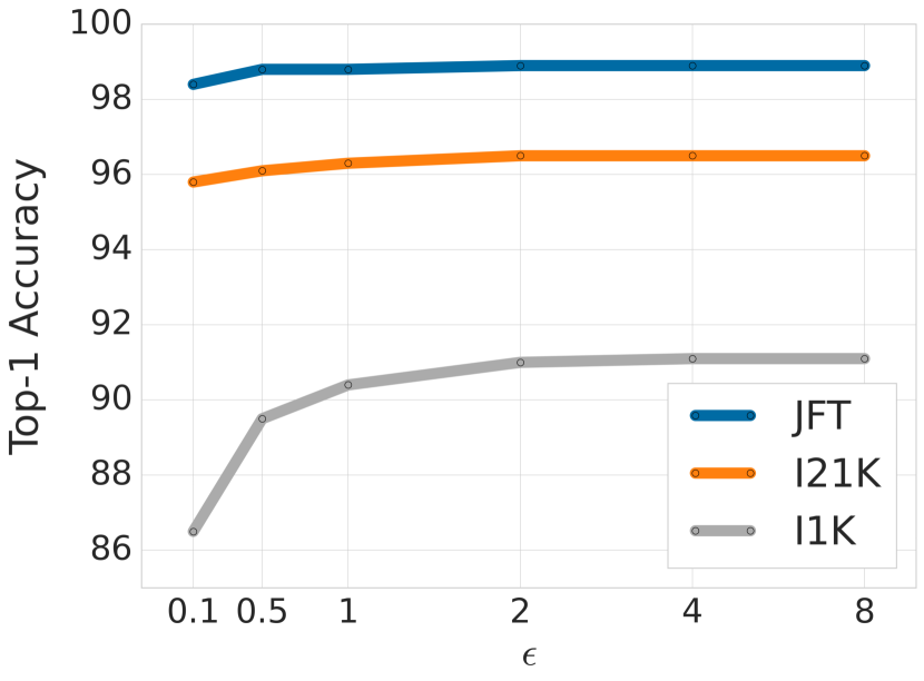
(a) CIFAR-10

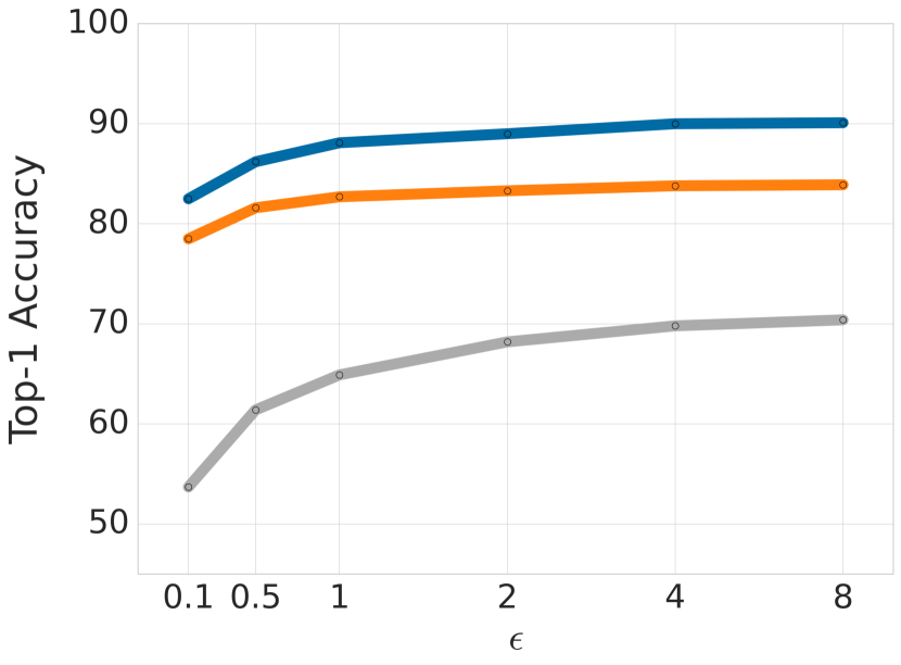
(b) CIFAR-100

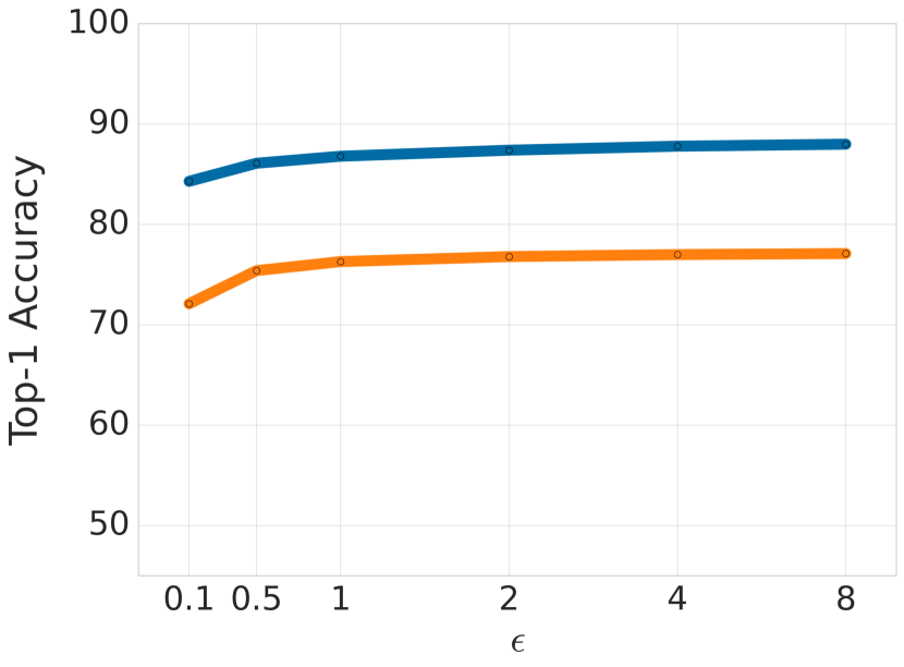
(c) ImageNet-1K

Figure 1: Comparison of top-1 accuracies with private fine-tuning using DP-FC method on all 3 datasets across a range of epsilons. We observe that better pre-training helps even more for lower values of epsilon (stricter privacy guarantee).

3.1 Better pre-training continues to improve private fine-tuning performance

We evaluate private fine-tuning performance on features extracted from pre-trained models of 2 sizes i.e. ViT-G/14 and ViT-B/16, pre-trained on 3 different datasets, namely JFT-3B, ImageNet-21K and ImageNet-1K. We do this to quantify the extent to which the representation quality is improved by increasing pre-training dataset in combination of model size. As shown in Figure 1, as the model size and pre-training dataset size is increased, we continue to see improvement in downstream private fine-tuning performance for all 3 datasets we consider. In addition, we make following observations from our results.

First, better pre-training can help even more at stricter privacy budgets. As shown in Figure 1, for both CIFAR-10 and CIFAR-100, when comparing features extracted from ViT-B/16 pre-trained with ImageNet-1K and features from ViT-G/14 pre-trained with JFT, the improvement in performance at $\varepsilon=1$ is larger than $\varepsilon=8$. We see a similar trend at even lower epsilons in Table 3 and Table 4.

Second, features extracted from off-the-shelf pre-trained models can suffice for DP. Except for the fact that we deduplicate all splits of our pre-training dataset with our fine-tuning datasets, we use the exact same procedure used to pre-train large vision models. This suggests that, in practice, a recipe where features extracted from large off-the-shelf vision model used to privately fine-tune a classifier can be quite effective for DP performance. Since there is no need for a special pre-trained model for use in DP, this considerably reduces the cost of training private image classifiers.

Lastly, private fine-tuning of high quality features closes the gap between private and non-private performance considerably. In the non-private setting, Zhai et al. (2021) obtain an impressive 90.45% top-1 accuracy by fine-tuning the whole ViT-G/14 model on ImageNet-1K dataset. We observe that even by fine-tuning just the last layer, we can obtain as much as 88.9% top-1 accuracy on ImageNet-1K from the same sized model. Thus the marginal benefit of fine-tuning the whole model is $<$2% even in the non-private case. In the private case, fine-tuning of pre-extracted features with DP-FC at $\varepsilon=8$ leads to state of the art 88% top-1 accuracy. On ViT-G/14, this represents $<2.5\%$ difference between best non-private and private performance. This is also just 3% below the best non-private accuracy of 91% on ImageNet-1K Yu et al. (2022b).

3.2 Better optimizers improve privacy-utility trade-off

We observe that the choice of optimizer can have a significant impact on the privacy-utility trade-off.

First, optimizers that work well in the large batch regime are better for private training. Even in the non-private setting, it is known that batch size is intimately tied to the optimization procedure and can lead to suboptimal use of resources if increased beyond a certain point while keeping number of epochs constant Goyal et al. (2017); You et al. (2017, 2019). The maximum batch size which can be used without jeopardizing the utility-compute trade-off is also heavily dependent on the choice of optimizer Zhang et al. (2019). Though in the private setting, several works have observed that increasing the batch size leads to improved privacy-utility trade-off Dormann et al. (2021); Li et al. (2014); Hoory et al. (2021). It is also empirically observed that the utility in large batch regime can be further improved by leveraging optimizers which work well in large batch regime, such as DP-Adam or DP-LAMB Anil et al. (2021); Mehta et al. (2022); Bu et al. (2022a). Second-order methods such as LS or Newton are also well-suited to the large-batch regime (they were developed and are typically used in the full-batch setting).

Second, optimizers with faster convergence rates are advantageous in the private setting, because they can reduce the number of epochs required for convergence. Indeed, in typical privacy analysis of iterative methods, the analysis works by composition over iterations, which means that the privacy penalty scales with the number of visitations of the data. Thus, in addition to the computational benefit, any improvement in convergence rate directly helps training with privacy because it requires less noise to be added under the same privacy constraints. We empirically observe that this reduction in noise in the case of DP-FC, in combination with sharing of the privatized Feature Covariance across classes and iterates, allow us to obtain better results with 10 epochs compared to even when using 100 epochs with DP-SGD.

4 Related Work

Differential privacy Dwork et al. (2006b) is a popular method to guarantee privacy in a quantifiable way in many data-driven applications. To achieve differential privacy in machine learning, tasks practitioners commonly train models with privatized variation of gradient descent, called DP-SGD (Song et al., 2013; Bassily et al., 2014; Abadi et al., 2016).

Despite theoretical guarantees, differentially private training has two major drawbacks which limits its wide adoption. First of all, differentially private training is slower compared to regular SGD. Training with DP-SGD is notably different from non-private training where the forward pass can be vectorized and only a single pre-accumulated gradient need be calculated and used per mini-batch. If implemented naively, this step alone increases the computational cost of DP training proportional to the batch size for a single step and the dimensionality of the model. Indeed, to address this, in several deep learning architectures, either its feasible to vectorize the computation (Subramani et al., 2020) or it is sometimes possible to bound the sensitivity of each example without calculating the gradient for every example separately, leading to a dramatic cost-reduction both in terms of memory and compute (Goodfellow, 2015; Li et al., 2022b; Bu et al., 2022a, d). Although, in our work this cost is minimal since we only train the last layer. We do note that computational burden can still be an issue for optimization schemes like DP-Newton in our work where we had to resort to feature clipping in order to produce bounds on sensitivity of the gradient and the hessian.

In addition to the computational cost, model trained with differentially privacy usually suffer from so-called “utility loss”, which means that accuracy (or any other quality metric) is worse (and sometimes significantly worse) compared to accuracy of non-private model (Dormann et al., 2021; Klause et al., 2022). Over the years, several lines of improvements have been proposed including adaptive clipping (Pichapati et al., 2019; Thakkar et al., 2019; Bu et al., 2022b; Golatkar et al., 2022), param-efficient finetuning Yu et al. (2022a); Mehta et al. (2022); Bu et al. (2022c); Cattan et al. (2022); Li et al. (2022a) and even leveraging intermediate checkpoints (De et al., 2022; Shejwalkar et al., 2022). One of the recent trends to improve utility of private models significantly involves various ideas related to transfer learning where previous works demonstrate improved performance in the setting where we have access to a large public or non-sensitive dataset of the same modality as the private data Kurakin et al. (2022); De et al. (2022); Mehta et al. (2022); Tramèr and Boneh (2021); Yu et al. (2022a); Li et al. (2022b); Kurakin et al. (2022); Hoory et al. (2021). Our work also leverages large pre-trained models in order to obtain high-quality features for private finetuning. In addition, similar to the works that focus on studying and reducing dimensionality of the model in the context of DP (Li et al., 2022a; Golatkar et al., 2022; Yu et al., 2021; Zhang et al., 2021; Zhou et al., 2020), we focus solely on learning just the last layer privately, which can be seen as an implicit way to reduce dimensionality.

In the context of differential privacy, several recent papers also advocate the use of large batch sizes in order to improve the privacy-utility tradeoff (Mehta et al., 2022; McMahan et al., 2018; Anil et al., 2021; Dormann et al., 2021; Hoory et al., 2021; Liu et al., 2021b; Kurakin et al., 2022). Even though this work explicitly does not explore the affect changing the batch size, the fact that we are able to obtain state of the art results in the full batch setting may point to the effectiveness of large batch sizes in the context of DP.

Further, our work also zooms in on differentially private linear and logistic regression. Several existing works have studied differential private convex optimization (Chaudhuri et al., 2011; Kifer et al., 2012; Song et al., 2013; Bassily et al., 2014; Wu et al., 2016; McMahan et al., 2017; Bassily et al., 2019; Iyengar et al., 2019; Feldman et al., 2020; Bassily et al., 2020; Song et al., 2020; Andrew et al., 2021). There is also a growing interest in the special case of linear regression (Smith et al., 2017; Sheffet, 2019; Liu et al., 2021a; Cai et al., 2021; Varshney et al., 2022) and even second order methods in the context of differential privacy Avella-Medina et al. (2021); Chien et al. (2021). In this work, we illustrate empirically the extent to which second order methods can help in DP. It would be quite interesting to see how other popular second order methods like Shampoo Gupta et al. (2018); Anil et al. (2020) would fare in the context of DP.

5 Limitations

This work leverages a large properietary dataset called JFT-3B to pre-train ViT-G/14 model in order to illustrate the benefits of scale on differential privacy with transfer learning. In order to make our work more generalizable and reproducible, we also include results with models pre-trained with ImageNet-21k and ImageNet-1k.

Another limitation of our work may be the fact that our pre-training dataset is largely in-distribution with the private fine-tuning datasets. We would like to argue that, in practice, this is still valuable since it illustrates the effectiveness of the approach, and helps estimate the utility of gathering a public dataset to pre-train on, given a sensitive dataset that one wants privacy guarantee over. Finally, out of distribution performance is an interesting research question even in the non-private setting and its exploration in the context of privacy can be a direction of very valuable future work.

In terms of societal impact, the biggest cost of this work is training the largest ViT-G model on a large dataset and its energy impact. However, we argue that our results ultimately point towards amortizing and increasingly leveraging already trained models for high-performance DP training, and thus potentially reducing the overall energy consumption.

6 Conclusion

In this work, we focus on private finetuning of image classification datasets using features extracted from a pre-trained model. Given that, with privacy, finetuning just on the features is significantly cheaper than finetuning the full model, we systematically explore optimization schemes which are perceived to be expensive in very high-dimensional settings and its effect on private finetuning performance. As illustrated on 3 finetuning datasets i.e. ImageNet-1k, CIFAR-10 and CIFAR-100, we find that DP-LS (Least Squares) outperforms DP-SGD with logistic regression, especially for lower values of epsilons. Given the intuition that 2nd order information may be the reason for superior performance of DP-LS, we also explore Newton’s method with Logistic Loss. Noticing that the amount of noise required by Newton’s method scales with the number of classes and iterations, we introduce an optimization scheme called DP-FC which replaces the hessian by the feature covariance matrix, that can be shared across classes and iterations. Using this insight, we demonstrate that it is indeed possible to get state of the art results by just finetuning the last layer of a pre-trained model with privacy constraints. Most remarkably, we obtain top-1 accuracy of 88% on ImageNet-1K under DP guarantee of (8, $8*10^{-7}$) and 84.3% under (0.1, $8*10^{-7}$). All of our results rely on leveraging well-understood procedures for transfer learning on standard architectures. We hope that our work significantly reduces the barrier in training private models.

Appendix A Appendix

Appendix B Algorithmic details

B.1 Privacy Analysis details for DP-SGD

The privacy parameters $(\varepsilon,\delta)$ are functions of $C$, $\sigma$, $|B_{t}|$, $|\mathcal{D}|$, and the total number of iterations $T$. DP-SGD algorithm involves setting the right clipping norm $C$ and the noise multiplier $\sigma$ given a privacy budget, batch and dataset size. The $(\varepsilon,\delta)$ guarantee is computed by analysis of the Gaussian Mechanism with privacy amplification by subsampling and composition across across iterations (Kasiviswanathan et al., 2008; Bassily et al., 2014; Abadi et al., 2016; Mironov, 2017; McMahan et al., 2017; Mironov et al., 2019; Erlingsson et al., 2019; Zhu and Wang, 2019; Feldman et al., 2020; Wang et al., 2020). Our implementation relies on Tensorflow Privacy codebase for conversion of $(\varepsilon,\delta)$ and clipping norm $C$ to/from noise multiplier $\sigma$. We rely on the default Rényi accountant implementation already open-sourced as part of Tensorflow Privacy library.

To put the epsilon-delta values in context, privacy guarantee for let’s say $\varepsilon\approx 4$ on ImageNet-1K satisfies a much stronger property of zCDP $\leq$ 1 (0.154 for $\varepsilon=4$) which is by now an industry standard.

Appendix C Pre-training Details

We conduct all our experiments in Jax (Bradbury et al., 2018; Frostig et al., 2018) is framework that leverages just-in-time compilation using XLA and does auto-vectorization of the backward pass. We leverage this functionality throughout our experiments. Finally, we conduct our experiments on TPUv4 architecture.

C.1 Pre-training with JFT-3B

Dataset. Contrary to Mehta et al. (2022); De et al. (2022), we use a smaller version of JFT, namely JFT-3B (instead of JFT-4B) for our pre-training. We do this to lower the risk of the project and follow Zhai et al. (2021) exactly for pre-training ViT-G/14 model. JFT-3B dataset consists of nearly 3 billion images, annotated with a class-hierarchy of around 30k labels via a semiautomatic pipeline. As done previously, we ignore the hierarchical aspect of the labels and use only the assigned labels as targets for multi-label classification via a sigmoid cross-entropy loss.

Deduplication. In order to both not inflate our results and break privacy guarantee offered by fine-tuning privately on ImageNet, we extend the deduplication process proposed by Kolesnikov et al. (2020) and deduplicate both JFT-3B with respect to all splits of ImageNet. We use a model based deduplication system which removes both exact and near-duplicates across common image transformation like crop, shift, resize etc.

Hyperparameters. At the pre-training stage, we follow Zhai et al. (2021) exactly and stick with the common practice of employing Adafactor optimizer with $\beta_{1}=0.9$ and $\beta_{2}=0.999$, with a batch size of 32768, dropout rate of 0.0, clip global norm of 1, and a high weight decay of 3.0 for the “head” and 0.03 for the “body”. In addition, we remove the additional $[class]$ token to save memory. Finally, all the models are pre-trained at resolution [224, 224], with inception crop followed by random horizontal flip pre-process. We also use reciprocal square-root schedule with a linear learning rate warmup of 10k steps. Finally, ViT-G/14 model was pre-trained using 2048 TPUv3 chips.

C.2 Pre-training with ImageNet21k and ImageNet1k

Datasets. ImageNet-21k is a superset of ImageNet-k with 21k classes and 14M images (Deng et al., 2009). Similar to before, in order to both not inflate our results and break privacy guarantee, we extend the deduplication process proposed by Kolesnikov et al. (2020) and deduplicate ImageNet-21k with respect to all splits of ImageNet-1k, CIFAR-10 and CIFAR-100. Similarly, we deduplicate ImageNet-1k with respect to all splits of CIFAR-10 and CIFAR-100.

Hyperparameters. At the pre-training stage, we stick with the common practice of employing Adam optimizer (even for ResNet) with $\beta_{1}=$ 0.9 and $\beta_{2}=$ 0.999, with a batch size of 4096. Unlike pre-training with JFT dataset, we follow recommendations from Steiner et al. (2021) to use AugReg strategy where we lower the weight decay to 0.1 (which gets multiplied by the learning rate) and don’t use dropout but instead use data augmentation strategy called medium1 which combines Mixup with $\alpha=0.2$ (Zhang et al., 2017) and RandAugment with $l=15$ and $m=2$ (Cubuk et al., 2020). We also use linear learning rate warmup until 10k steps and linearly decay it until the end. Our model is pre-trained with 224x224-sized images.

Model	Dataset	Epochs	Base $\eta$	TPU v4 hours
ViT-B/16	ImageNet-21k	300	$10^{-3}$	2.7k
ViT-B/16	Imagenet-1K	300	$10^{-3}$	0.4k

Table 5: Pre-training hyperparams. We used batch size of 4096, learning rate warmup of 10k steps and then linear decay. Additionally, we set dropout rate to 0.0, clip global norm to 1 and weight decay to 0.0001. We use images of resolution 224x224. Note that we intentionally keep the model size the same to illustrate the effect of larger pre-training dataset and its effect on private fine-tuning.

Appendix D Finetuning Details

D.1 Datasets

ImageNet-1k We fine-tune on ImageNet train split and present the Top-1 accuracies we obtain from the official test split. Following Mehta et al. (2022), we used images of input resolution 256x256 which is central cropped from a resolution of 384x384. Note that this is slightly lower resolution and without Inception Crop (Szegedy et al., 2015) which is typically done in non-private setting. Finally, for training with DP, we fixed $\delta$ to be 8e-7.

CIFAR-10 and CIFAR-100 Similar to above, we fine-tune on train split and present the Top-1 accuracies we obtain from the official test split. We also changed the input resolution to 256x256 which is central cropped from an image of resolution 384x384. Again, this may look a little unusual at first for CIFAR-10 and CIFAR-100 since the original resolution of the images is 32x32. But we first upsample them to 384x384 and then central crop them. We found that using higher resolution images made a big difference in performance (even in non-private setting), especially when using features from a pre-trained model. Finally, for training with DP, we fixed $\delta$ to be 1e-5.

D.2 DP-Adam hyperparameters

Model	Pre-training DS	Fine-tuning DS	$\eta$	$\lambda$	DP Clipping Norm ($C$)
ViT-G/14	JFT-3B	ImageNet-1k	$[10^{-8},10^{8}]$	$[10^{-8},10^{8}]$	1.0
ViT-G/14	JFT-3B	CIFAR-10	$[10^{-8},10^{8}]$	$[10^{-8},10^{8}]$	0.005
ViT-G/14	JFT-3B	CIFAR-100	$[10^{-8},10^{8}]$	$[10^{-8},10^{8}]$	0.005
ViT-B/16	ImageNet-21k	ImageNet-1k	$[10^{-8},10^{8}]$	$[10^{-8},10^{8}]$	0.005
ViT-B/16	ImageNet-21k	CIFAR-10	$[10^{-8},10^{8}]$	$[10^{-8},10^{8}]$	0.005
ViT-B/16	ImageNet-21k	CIFAR-100	$[10^{-8},10^{8}]$	$[10^{-8},10^{8}]$	0.005
ViT-B/16	ImageNet-1k	CIFAR-10	$[10^{-8},10^{8}]$	$[10^{-8},10^{8}]$	0.005
ViT-B/16	ImageNet-1k	CIFAR-100	$[10^{-8},10^{8}]$	$[10^{-8},10^{8}]$	0.005

Table 6: Fine-tuning hyperparams for DP-Adam. All models are trained in full-batch setting with a constant learning rate and no dropout. When training the models with DP, we replace the global clipping with per example clipping norm as specified in the table. Following Mehta et al. (2022), we set initial weights to 0.0, bias to -10.0 and train with sigmoid cross-entropy loss. Note that we employed a Bayesian optimization package called Vizier (Golovin et al., 2017; Song et al., 2022) and used a total of 200 trials for jointly tuning both the learning rate and weight decay as specified in the table.

D.3 DP-LS hyperparameters

Model	Pre-training DS	Fine-tuning DS	$\alpha$	$\lambda$	DP Clipping Norm ($C$)
ViT-G/14	JFT-3B	ImageNet-1k	$[10^{-8},10^{8}]$	$[10^{-8},10^{8}]$	1.0
ViT-G/14	JFT-3B	CIFAR-10	$[10^{-8},10^{8}]$	$[10^{-8},10^{8}]$	0.005
ViT-G/14	JFT-3B	CIFAR-100	$[10^{-8},10^{8}]$	$[10^{-8},10^{8}]$	0.005
ViT-B/16	ImageNet-21k	ImageNet-1k	$[10^{-8},10^{8}]$	$[10^{-8},10^{8}]$	0.005
ViT-B/16	ImageNet-21k	CIFAR-10	$[10^{-8},10^{8}]$	$[10^{-8},10^{8}]$	0.005
ViT-B/16	ImageNet-21k	CIFAR-100	$[10^{-8},10^{8}]$	$[10^{-8},10^{8}]$	0.005
ViT-B/16	ImageNet-1k	CIFAR-10	$[10^{-8},10^{8}]$	$[10^{-8},10^{8}]$	0.005
ViT-B/16	ImageNet-1k	CIFAR-100	$[10^{-8},10^{8}]$	$[10^{-8},10^{8}]$	0.005

Table 7: Fine-tuning hyperparams for DP-LS. All models are trained in full-batch setting. When training the models with DP, we replace the global clipping with per example clipping norm as specified in the table. Specific to DP-LS, we clip the RHS with $C$ and the gramians with $C^{2}$. Interestingly, least squares is invariant to the starting weights which takes an important confounding factor away from the private training procedure. Similar to DP-Adam, we employed a Bayesian optimization package called Vizier (Golovin et al., 2017; Song et al., 2022) and used a total of 200 trials for jointly tuning both the $\alpha$ and weight decay as specified in the table.

D.4 DP-Newton hyperparameters

Model	Pre-training DS	Fine-tuning DS	$\eta$	$\lambda$	DP Clipping Norm ($C$)
ViT-G/14	JFT-3B	ImageNet-1k	$[10^{-8},10^{8}]$	$[10^{-8},10^{8}]$	1.0
ViT-G/14	JFT-3B	CIFAR-10	$[10^{-8},10^{8}]$	$[10^{-8},10^{8}]$	0.005
ViT-G/14	JFT-3B	CIFAR-100	$[10^{-8},10^{8}]$	$[10^{-8},10^{8}]$	0.005
ViT-B/16	ImageNet-21k	ImageNet-1k	$[10^{-8},10^{8}]$	$[10^{-8},10^{8}]$	0.005
ViT-B/16	ImageNet-21k	CIFAR-10	$[10^{-8},10^{8}]$	$[10^{-8},10^{8}]$	0.005
ViT-B/16	ImageNet-21k	CIFAR-100	$[10^{-8},10^{8}]$	$[10^{-8},10^{8}]$	0.005
ViT-B/16	ImageNet-1k	CIFAR-10	$[10^{-8},10^{8}]$	$[10^{-8},10^{8}]$	0.005
ViT-B/16	ImageNet-1k	CIFAR-100	$[10^{-8},10^{8}]$	$[10^{-8},10^{8}]$	0.005

Table 8: Fine-tuning hyperparams for DP-Newton. All models are trained in full-batch setting with a constant learning rate and no dropout. When training the models with DP, we replace the global clipping with per example clipping norm as specified in the table. Specific to DP-Newton, we clip the features instead of the gradient and the Hessian. We do this save on computational cost since now we don’t need to explicitly compute per-example gradient and the Hessian. For the privacy analysis, we use the clipping norm $C$ to sanitize the gradient and $\frac{C^{2}}{4.0}$ for the Hessian. Following Mehta et al. (2022), we set initial weights to 0.0 and train with sigmoid cross-entropy loss. We employed a Bayesian optimization package called Vizier (Golovin et al., 2017; Song et al., 2022) and used a total of 300 trials for jointly tuning both the learning rate and weight decay as specified in the table.

D.5 DP-FC hyperparameters

Model	Pretraining DS	Finetuning DS	$\eta$	$\lambda$	DP Clipping Norm ($C$)
ViT-G/14	JFT-3B	ImageNet-1k	$[10^{-8},10^{8}]$	$[10^{-8},10^{8}]$	1.0
ViT-G/14	JFT-3B	CIFAR-10	$[10^{-8},10^{8}]$	$[10^{-8},10^{8}]$	0.005
ViT-G/14	JFT-3B	CIFAR-100	$[10^{-8},10^{8}]$	$[10^{-8},10^{8}]$	0.005
ViT-B/16	ImageNet-21k	ImageNet-1k	$[10^{-8},10^{8}]$	$[10^{-8},10^{8}]$	0.005
ViT-B/16	ImageNet-21k	CIFAR-10	$[10^{-8},10^{8}]$	$[10^{-8},10^{8}]$	0.005
ViT-B/16	ImageNet-21k	CIFAR-100	$[10^{-8},10^{8}]$	$[10^{-8},10^{8}]$	0.005
ViT-B/16	ImageNet-1k	CIFAR-10	$[10^{-8},10^{8}]$	$[10^{-8},10^{8}]$	0.005
ViT-B/16	ImageNet-1k	CIFAR-100	$[10^{-8},10^{8}]$	$[10^{-8},10^{8}]$	0.005

Table 9: Fine-tuning hyperparams for DP-FC. All models are trained in full-batch setting with a constant learning rate and no dropout. When training the models with DP, we replace the global clipping with per example clipping norm as specified in the table. Specific to DP-FC, we clip the per-example gradients with clipping norm $C$ and $C^{2}$ for the gramian which is shared across classes and iterations. Following Mehta et al. (2022), we set initial weights to 0.0, set initial bias to -10.0 and train with sigmoid cross-entropy loss. We employed a Bayesian optimization package called Vizier (Golovin et al., 2017; Song et al., 2022) and used a total of 200 trials for jointly tuning both the learning rate and weight decay as specified in the table.

References

- Abadi et al. (2016) Martín Abadi, Andy Chu, Ian J. Goodfellow, H. Brendan McMahan, Ilya Mironov, Kunal Talwar, and Li Zhang. Deep learning with differential privacy. In Proc. of the 2016 ACM SIGSAC Conf. on Computer and Communications Security (CCS’16), pages 308–318, 2016.
- Andrew et al. (2021) Galen Andrew, Om Thakkar, Hugh Brendan McMahan, and Swaroop Ramaswamy. Differentially private learning with adaptive clipping. In A. Beygelzimer, Y. Dauphin, P. Liang, and J. Wortman Vaughan, editors, Advances in Neural Information Processing Systems, 2021. URL https://openreview.net/forum?id=RUQ1zwZR8_.
- Anil et al. (2020) Rohan Anil, Vineet Gupta, Tomer Koren, Kevin Regan, and Yoram Singer. Scalable second order optimization for deep learning, 2020.
- Anil et al. (2021) Rohan Anil, Badih Ghazi, Vineet Gupta, Ravi Kumar, and Pasin Manurangsi. Large-scale differentially private BERT. CoRR, abs/2108.01624, 2021. URL https://arxiv.org/abs/2108.01624.
- Avella-Medina et al. (2021) Marco Avella-Medina, Casey Bradshaw, and Po-Ling Loh. Differentially private inference via noisy optimization, 2021.
- Balle et al. (2022) Borja Balle, Giovanni Cherubin, and Jamie Hayes. Reconstructing training data with informed adversaries, 2022.
- Bassily et al. (2014) Raef Bassily, Adam Smith, and Abhradeep Thakurta. Private empirical risk minimization: Efficient algorithms and tight error bounds. In Proc. of the 2014 IEEE 55th Annual Symp. on Foundations of Computer Science (FOCS), pages 464–473, 2014.
- Bassily et al. (2019) Raef Bassily, Vitaly Feldman, Kunal Talwar, and Abhradeep Guha Thakurta. Private stochastic convex optimization with optimal rates. In Hanna M. Wallach, Hugo Larochelle, Alina Beygelzimer, Florence d’Alché-Buc, Emily B. Fox, and Roman Garnett, editors, Advances in Neural Information Processing Systems 32: Annual Conference on Neural Information Processing Systems 2019, NeurIPS 2019, 8-14 December 2019, Vancouver, BC, Canada, pages 11279–11288, 2019. URL http://papers.nips.cc/paper/9306-private-stochastic-convex-optimization-with-optimal-rates.
- Bassily et al. (2020) Raef Bassily, Vitaly Feldman, Cristóbal Guzmán, and Kunal Talwar. Stability of stochastic gradient descent on nonsmooth convex losses. In NeurIPS, 2020. URL https://proceedings.neurips.cc/paper/2020/hash/2e2c4bf7ceaa4712a72dd5ee136dc9a8-Abstract.html.
- Bradbury et al. (2018) James Bradbury, Roy Frostig, Peter Hawkins, Matthew James Johnson, Chris Leary, Dougal Maclaurin, and Skye Wanderman-Milne. JAX: composable transformations of Python+NumPy programs, 2018. URL http://github.com/google/jax.
- Brock et al. (2021) Andrew Brock, Soham De, and Samuel L Smith. Characterizing signal propagation to close the performance gap in unnormalized resnets. In International Conference on Learning Representations, 2021. URL https://openreview.net/forum?id=IX3Nnir2omJ.
- Bu et al. (2022a) Zhiqi Bu, Jialin Mao, and Shiyun Xu. Scalable and efficient training of large convolutional neural networks with differential privacy, 2022a.
- Bu et al. (2022b) Zhiqi Bu, Yu-Xiang Wang, Sheng Zha, and George Karypis. Automatic clipping: Differentially private deep learning made easier and stronger. ArXiv, abs/2206.07136, 2022b.
- Bu et al. (2022c) Zhiqi Bu, Yu-Xiang Wang, Sheng Zha, and George Karypis. Differentially private bias-term only fine-tuning of foundation models. ArXiv, abs/2210.00036, 2022c.
- Bu et al. (2022d) Zhiqi Bu, Yu-Xiang Wang, Sheng Zha, and George Karypis. Differentially private optimization on large model at small cost. ArXiv, abs/2210.00038, 2022d.
- Bun and Steinke (2016) Mark Bun and Thomas Steinke. Concentrated differential privacy: Simplifications, extensions, and lower bounds. In Theory of Cryptography Conference, pages 635–658. Springer, 2016.
- Cai et al. (2021) T Tony Cai, Yichen Wang, and Linjun Zhang. The cost of privacy: Optimal rates of convergence for parameter estimation with differential privacy. The Annals of Statistics, 49(5):2825–2850, 2021.
- Carlini et al. (2019) Nicholas Carlini, Chang Liu, Úlfar Erlingsson, Jernej Kos, and Dawn Song. The secret sharer: Evaluating and testing unintended memorization in neural networks. In Proceedings of the 28th USENIX Conference on Security Symposium, 2019.
- Carlini et al. (2021) Nicholas Carlini, Florian Tramèr, Eric Wallace, Matthew Jagielski, Ariel Herbert-Voss, Katherine Lee, Adam Roberts, Tom Brown, Dawn Song, Úlfar Erlingsson, Alina Oprea, and Colin Raffel. Extracting training data from large language models. In USENIX Security, 2021.
- Cattan et al. (2022) Yannis Cattan, Christopher A. Choquette-Choo, Nicolas Papernot, and Abhradeep Thakurta. Fine-tuning with differential privacy necessitates an additional hyperparameter search. ArXiv, abs/2210.02156, 2022.
- Chaudhuri et al. (2011) Kamalika Chaudhuri, Claire Monteleoni, and Anand D Sarwate. Differentially private empirical risk minimization. Journal of Machine Learning Research, 12(Mar):1069–1109, 2011.
- Chien et al. (2021) Steve Chien, Prateek Jain, Walid Krichene, Steffen Rendle, Shuang Song, Abhradeep Thakurta, and Li Zhang. Private alternating least squares: Practical private matrix completion with tighter rates, 2021.
- Choquette-Choo et al. (2020) Christopher A. Choquette-Choo, Florian Tramer, Nicholas Carlini, and Nicolas Papernot. Label-only membership inference attacks, 2020.
- Cubuk et al. (2020) Ekin D. Cubuk, Barret Zoph, Jonathon Shlens, and Quoc V. Le. Randaugment: Practical automated data augmentation with a reduced search space. 2020 IEEE/CVF Conference on Computer Vision and Pattern Recognition Workshops (CVPRW), Jun 2020. doi: 10.1109/cvprw50498.2020.00359. URL http://dx.doi.org/10.1109/CVPRW50498.2020.00359.
- De et al. (2022) Soham De, Leonard Berrada, Jamie Hayes, Samuel L. Smith, and Borja Balle. Unlocking high-accuracy differentially private image classification through scale, 2022. URL https://arxiv.org/abs/2204.13650.
- Deng et al. (2009) Jia Deng, Wei Dong, Richard Socher, Li-Jia Li, Kai Li, and Li Fei-Fei. Imagenet: A large-scale hierarchical image database. In 2009 IEEE conference on computer vision and pattern recognition, pages 248–255. Ieee, 2009.
- Dormann et al. (2021) Friedrich Dormann, Osvald Frisk, Lars Norvang Andersen, and Christian Fischer Pedersen. Not all noise is accounted equally: How differentially private learning benefits from large sampling rates. 2021 IEEE 31st International Workshop on Machine Learning for Signal Processing (MLSP), Oct 2021. doi: 10.1109/mlsp52302.2021.9596307. URL http://dx.doi.org/10.1109/mlsp52302.2021.9596307.
- Dosovitskiy et al. (2021) Alexey Dosovitskiy, Lucas Beyer, Alexander Kolesnikov, Dirk Weissenborn, Xiaohua Zhai, Thomas Unterthiner, Mostafa Dehghani, Matthias Minderer, Georg Heigold, Sylvain Gelly, Jakob Uszkoreit, and Neil Houlsby. An image is worth 16x16 words: Transformers for image recognition at scale. In International Conference on Learning Representations, 2021. URL https://openreview.net/forum?id=YicbFdNTTy.
- Dwork et al. (2006a) Cynthia Dwork, Krishnaram Kenthapadi, Frank McSherry, Ilya Mironov, and Moni Naor. Our data, ourselves: Privacy via distributed noise generation. In Advances in Cryptology—EUROCRYPT, pages 486–503, 2006a.
- Dwork et al. (2006b) Cynthia Dwork, Frank McSherry, Kobbi Nissim, and Adam Smith. Calibrating noise to sensitivity in private data analysis. In Shai Halevi and Tal Rabin, editors, Theory of Cryptography, 2006b.
- Erlingsson et al. (2019) Úlfar Erlingsson, Vitaly Feldman, Ilya Mironov, Ananth Raghunathan, Kunal Talwar, and Abhradeep Thakurta. Amplification by shuffling: From local to central differential privacy via anonymity. In Timothy M. Chan, editor, Proceedings of the Thirtieth Annual ACM-SIAM Symposium on Discrete Algorithms, SODA 2019, San Diego, California, USA, January 6-9, 2019, pages 2468–2479. SIAM, 2019. doi: 10.1137/1.9781611975482.151. URL https://doi.org/10.1137/1.9781611975482.151.
- Feldman et al. (2020) Vitaly Feldman, Audra McMillan, and Kunal Talwar. Hiding among the clones: A simple and nearly optimal analysis of privacy amplification by shuffling. arXiv preprint arXiv:2012.12803, 2020.
- Frostig et al. (2018) Roy Frostig, Matthew Johnson, and Chris Leary. Compiling machine learning programs via high-level tracing. 2018. URL https://mlsys.org/Conferences/doc/2018/146.pdf.
- Golatkar et al. (2022) Aditya Golatkar, Alessandro Achille, Yu-Xiang Wang, Aaron Roth, Michael Kearns, and Stefano Soatto. Mixed differential privacy in computer vision. 2022 IEEE/CVF Conference on Computer Vision and Pattern Recognition (CVPR), Jun 2022. doi: 10.1109/cvpr52688.2022.00819. URL http://dx.doi.org/10.1109/CVPR52688.2022.00819.
- Golovin et al. (2017) Daniel Golovin, Benjamin Solnik, Subhodeep Moitra, Greg Kochanski, John Elliot Karro, and D. Sculley, editors. Google Vizier: A Service for Black-Box Optimization, 2017. URL http://www.kdd.org/kdd2017/papers/view/google-vizier-a-service-for-black-box-optimization.
- Goodfellow (2015) Ian J. Goodfellow. Efficient per-example gradient computations. ArXiv, abs/1510.01799, 2015.
- Goyal et al. (2017) Priya Goyal, Piotr Dollár, Ross B. Girshick, Pieter Noordhuis, Lukasz Wesolowski, Aapo Kyrola, Andrew Tulloch, Yangqing Jia, and Kaiming He. Accurate, large minibatch SGD: training imagenet in 1 hour, 2017.
- Gupta et al. (2018) Vineet Gupta, Tomer Koren, and Yoram Singer. Shampoo: Preconditioned stochastic tensor optimization, 2018.
- Hoory et al. (2021) Shlomo Hoory, Amir Feder, Avichai Tendler, Sofia Erell, Alon Cohen, Itay Laish, Hootan Nakhost, Uri Stemmer, Ayelet Benjamini, Avinatan Hassidim, and Yossi Matias. Learning and evaluating a differentially private pre-trained language model. In Findings of the Association for Computational Linguistics: EMNLP 2021, pages 1178–1189, Punta Cana, Dominican Republic, 2021. URL https://aclanthology.org/2021.findings-emnlp.102/.
- Hu et al. (2008) Yifan Hu, Yehuda Koren, and Chris Volinsky. Collaborative filtering for implicit feedback datasets. In Proceedings of the 2008 Eighth IEEE International Conference on Data Mining, ICDM ’08, pages 263–272, 2008.
- Iyengar et al. (2019) Roger Iyengar, Joseph P Near, Dawn Song, Om Thakkar, Abhradeep Thakurta, and Lun Wang. Towards practical differentially private convex optimization. In 2019 IEEE Symposium on Security and Privacy (SP), 2019.
- Kasiviswanathan et al. (2008) Shiva Prasad Kasiviswanathan, Homin K. Lee, Kobbi Nissim, Sofya Raskhodnikova, and Adam D. Smith. What can we learn privately? In 49th Annual IEEE Symp. on Foundations of Computer Science (FOCS), pages 531–540, 2008.
- Kifer et al. (2012) Daniel Kifer, Adam Smith, and Abhradeep Thakurta. Private convex empirical risk minimization and high-dimensional regression. In Conference on Learning Theory, pages 25–1, 2012.
- Klause et al. (2022) Helena Klause, Alexander Ziller, Daniel Rueckert, Kerstin Hammernik, and Georgios Kaissis. Differentially private training of residual networks with scale normalisation, 2022.
- Kolesnikov et al. (2020) Alexander Kolesnikov, Lucas Beyer, Xiaohua Zhai, Joan Puigcerver, Jessica Yung, Sylvain Gelly, and Neil Houlsby. Big transfer (bit): General visual representation learning. Lecture Notes in Computer Science, page 491–507, 2020. ISSN 1611-3349. doi: 10.1007/978-3-030-58558-7˙29. URL http://dx.doi.org/10.1007/978-3-030-58558-7_29.
- Koren and Bell (2015) Yehuda Koren and Robert Bell. Advances in collaborative filtering. Recommender systems handbook, pages 77–118, 2015.
- Kurakin et al. (2022) Alexey Kurakin, Shuang Song, Steve Chien, Roxana Geambasu, Andreas Terzis, and Abhradeep Thakurta. Toward training at imagenet scale with differential privacy, 2022.
- Li et al. (2014) Mu Li, Tong Zhang, Yuqiang Chen, and Alexander J. Smola. Efficient mini-batch training for stochastic optimization. In Proceedings of the 20th ACM SIGKDD International Conference on Knowledge Discovery and Data Mining, KDD ’14, page 661–670, New York, NY, USA, 2014. Association for Computing Machinery. ISBN 9781450329569. doi: 10.1145/2623330.2623612. URL https://doi.org/10.1145/2623330.2623612.
- Li et al. (2022a) Xuechen Li, Daogao Liu, Tatsunori Hashimoto, Huseyin A. Inan, Janardhan Kulkarni, Yin Tat Lee, and Abhradeep Thakurta. When does differentially private learning not suffer in high dimensions? ArXiv, abs/2207.00160, 2022a.
- Li et al. (2022b) Xuechen Li, Florian Tramer, Percy Liang, and Tatsunori Hashimoto. Large language models can be strong differentially private learners. In International Conference on Learning Representations, 2022b. URL https://openreview.net/forum?id=bVuP3ltATMz.
- Liu et al. (2021a) Xiyang Liu, Weihao Kong, and Sewoong Oh. Differential privacy and robust statistics in high dimensions, 2021a.
- Liu et al. (2021b) Yugeng Liu, Rui Wen, Xinlei He, Ahmed Salem, Zhikun Zhang, Michael Backes, Emiliano De Cristofaro, Mario Fritz, and Yang Zhang. Ml-doctor: Holistic risk assessment of inference attacks against machine learning models, 2021b.
- McMahan et al. (2017) H Brendan McMahan, Daniel Ramage, Kunal Talwar, and Li Zhang. Learning differentially private recurrent language models. arXiv preprint arXiv:1710.06963, 2017.
- McMahan et al. (2018) H. Brendan McMahan, Daniel Ramage, Kunal Talwar, and Li Zhang. Learning differentially private recurrent language models. In International Conference on Learning Representations, 2018. URL https://openreview.net/forum?id=BJ0hF1Z0b.
- Mehta et al. (2022) Harsh Mehta, Abhradeep Thakurta, Alexey Kurakin, and Ashok Cutkosky. Large scale transfer learning for differentially private image classification. 2022.
- Mironov (2017) Ilya Mironov. Rényi differential privacy. In 2017 IEEE 30th Computer Security Foundations Symposium (CSF), pages 263–275. IEEE, 2017.
- Mironov et al. (2019) Ilya Mironov, Kunal Talwar, and Li Zhang. Rényi differential privacy of the sampled gaussian mechanism, 2019.
- Nasr et al. (2021) Milad Nasr, Shuang Songi, Abhradeep Thakurta, Nicolas Papernot, and Nicholas Carlin. Adversary instantiation: Lower bounds for differentially private machine learning. 2021 IEEE Symposium on Security and Privacy (SP), May 2021. doi: 10.1109/sp40001.2021.00069. URL http://dx.doi.org/10.1109/sp40001.2021.00069.
- Pichapati et al. (2019) Venkatadheeraj Pichapati, Ananda Theertha Suresh, Felix X Yu, Sashank J Reddi, and Sanjiv Kumar. Adaclip: Adaptive clipping for private sgd. arXiv preprint arXiv:1908.07643, 2019.
- Sheffet (2019) Or Sheffet. Old techniques in differentially private linear regression. In Aurélien Garivier and Satyen Kale, editors, Proceedings of the 30th International Conference on Algorithmic Learning Theory, volume 98 of Proceedings of Machine Learning Research, pages 789–827. PMLR, 22–24 Mar 2019. URL https://proceedings.mlr.press/v98/sheffet19a.html.
- Shejwalkar et al. (2022) Virat Shejwalkar, Arun Ganesh, Rajiv Mathews, Om Thakkar, and Abhradeep Thakurta. Recycling scraps: Improving private learning by leveraging intermediate checkpoints. ArXiv, abs/2210.01864, 2022.
- Shokri et al. (2017) Reza Shokri, Marco Stronati, Congzheng Song, and Vitaly Shmatikov. Membership inference attacks against machine learning models. In 2017 IEEE Symposium on Security and Privacy (SP), pages 3–18, 2017.
- Smith et al. (2017) Adam Smith, Abhradeep Thakurta, and Jalaj Upadhyay. Is interaction necessary for distributed private learning? In 2017 IEEE Symposium on Security and Privacy (SP), pages 58–77. IEEE, 2017.
- Song et al. (2013) Shuang Song, Kamalika Chaudhuri, and Anand D Sarwate. Stochastic gradient descent with differentially private updates. In 2013 IEEE Global Conference on Signal and Information Processing, pages 245–248. IEEE, 2013.
- Song et al. (2020) Shuang Song, Om Thakkar, and Abhradeep Thakurta. Characterizing private clipped gradient descent on convex generalized linear problems. arXiv preprint arXiv:2006.06783, 2020.
- Song et al. (2022) Xingyou Song, Sagi Perel, Chansoo Lee, Greg Kochanski, and Daniel Golovin. Open source vizier: Distributed infrastructure and api for reliable and flexible blackbox optimization. In Automated Machine Learning Conference, Systems Track (AutoML-Conf Systems), 2022.
- Steiner et al. (2021) Andreas Steiner, Alexander Kolesnikov, Xiaohua Zhai, Ross Wightman, Jakob Uszkoreit, and Lucas Beyer. How to train your vit? data, augmentation, and regularization in vision transformers, 2021.
- Subramani et al. (2020) Pranav Subramani, Nicholas Vadivelu, and Gautam Kamath. Enabling fast differentially private sgd via just-in-time compilation and vectorization. arXiv preprint arXiv:2010.09063, 2020.
- Szegedy et al. (2015) Christian Szegedy, Wei Liu, Yangqing Jia, Pierre Sermanet, Scott E. Reed, Dragomir Anguelov, D. Erhan, Vincent Vanhoucke, and Andrew Rabinovich. Going deeper with convolutions. 2015 IEEE Conference on Computer Vision and Pattern Recognition (CVPR), pages 1–9, 2015.
- Thakkar et al. (2019) Om Thakkar, Galen Andrew, and H Brendan McMahan. Differentially private learning with adaptive clipping. arXiv preprint arXiv:1905.03871, 2019.
- Tolstikhin et al. (2021) Ilya Tolstikhin, Neil Houlsby, Alexander Kolesnikov, Lucas Beyer, Xiaohua Zhai, Thomas Unterthiner, Jessica Yung, Andreas Peter Steiner, Daniel Keysers, Jakob Uszkoreit, Mario Lucic, and Alexey Dosovitskiy. MLP-mixer: An all-MLP architecture for vision. In A. Beygelzimer, Y. Dauphin, P. Liang, and J. Wortman Vaughan, editors, Advances in Neural Information Processing Systems, 2021. URL https://openreview.net/forum?id=EI2KOXKdnP.
- Tramèr and Boneh (2021) Florian Tramèr and Dan Boneh. Differentially private learning needs better features (or much more data). In International Conference on Learning Representations, 2021. URL https://openreview.net/forum?id=YTWGvpFOQD-.
- Varshney et al. (2022) Prateek Varshney, Abhradeep Thakurta, and Prateek Jain. (nearly) optimal private linear regression for sub-gaussian data via adaptive clipping. In Po-Ling Loh and Maxim Raginsky, editors, Proceedings of Thirty Fifth Conference on Learning Theory, volume 178 of Proceedings of Machine Learning Research, pages 1126–1166. PMLR, 02–05 Jul 2022. URL https://proceedings.mlr.press/v178/varshney22a.html.
- Wang et al. (2020) Yu-Xiang Wang, Borja Balle, and Shiva Kasiviswanathan. Subsampled rényi differential privacy and analytical moments accountant. Journal of Privacy and Confidentiality, 10(2), Jun 2020. ISSN 2575-8527. doi: 10.29012/jpc.723. URL http://dx.doi.org/10.29012/jpc.723.
- Wu et al. (2016) Xi Wu, Fengan Li, Arun Kumar, Kamalika Chaudhuri, Somesh Jha, and Jeffrey F. Naughton. Bolt-on differential privacy for scalable stochastic gradient descent-based analytics, 2016.
- You et al. (2017) Yang You, Igor Gitman, and Boris Ginsburg. Scaling SGD batch size to 32k for imagenet training, 2017.
- You et al. (2019) Yang You, Jing Li, Sashank Reddi, Jonathan Hseu, Sanjiv Kumar, Srinadh Bhojanapalli, Xiaodan Song, James Demmel, Kurt Keutzer, and Cho-Jui Hsieh. Large batch optimization for deep learning: Training bert in 76 minutes, 2019.
- Yu et al. (2021) Da Yu, Huishuai Zhang, Wei Chen, and Tie-Yan Liu. Do not let privacy overbill utility: Gradient embedding perturbation for private learning. In 9th International Conference on Learning Representations, ICLR 2021, Virtual Event, Austria, May 3-7, 2021. OpenReview.net, 2021. URL https://openreview.net/forum?id=7aogOj_VYO0.
- Yu et al. (2022a) Da Yu, Saurabh Naik, Arturs Backurs, Sivakanth Gopi, Huseyin A. Inan, Gautam Kamath, Janardhan Kulkarni, Yin Tat Lee, Andre Manoel, Lukas Wutschitz, Sergey Yekhanin, and Huishuai Zhang. Differentially private fine-tuning of language models. ArXiv, abs/2110.06500, 2022a.
- Yu et al. (2022b) Jiahui Yu, Zirui Wang, Vijay Vasudevan, Legg Yeung, Mojtaba Seyedhosseini, and Yonghui Wu. Coca: Contrastive captioners are image-text foundation models, 2022b.
- Zhai et al. (2021) Xiaohua Zhai, Alexander Kolesnikov, Neil Houlsby, and Lucas Beyer. Scaling vision transformers, 2021.
- Zhang et al. (2019) Guodong Zhang, Lala Li, Zachary Nado, James Martens, Sushant Sachdeva, George E. Dahl, Christopher J. Shallue, and Roger Grosse. Which algorithmic choices matter at which batch sizes? insights from a noisy quadratic model, 2019.
- Zhang et al. (2017) Hongyi Zhang, Moustapha Cisse, Yann N. Dauphin, and David Lopez-Paz. mixup: Beyond empirical risk minimization, 2017.
- Zhang et al. (2021) Huanyu Zhang, Ilya Mironov, and Meisam Hejazinia. Wide network learning with differential privacy, 2021.
- Zhou et al. (2020) Yingxue Zhou, Zhiwei Steven Wu, and Arindam Banerjee. Bypassing the ambient dimension: Private sgd with gradient subspace identification, 2020.
- Zhu and Wang (2019) Yuqing Zhu and Yu-Xiang Wang. Poission subsampled rényi differential privacy. In International Conference on Machine Learning, pages 7634–7642. PMLR, 2019.