CPPF++: Uncertainty-Aware Sim2Real Object Pose Estimation by Vote Aggregation

Abstract

Object pose estimation constitutes a critical area within the domain of 3D vision. While contemporary state-of-the-art methods that leverage real-world pose annotations have demonstrated commendable performance, the procurement of such real-world training data incurs substantial costs. This paper focuses on a specific setting wherein only 3D CAD models are utilized as a priori knowledge, devoid of any background or clutter information. We introduce a novel method, CPPF++, designed for sim-to-real pose estimation. This method builds upon the foundational point-pair voting scheme of CPPF, reconceptualizing it through a probabilistic lens. To address the challenge of voting collision, we model voting uncertainty by estimating the probabilistic distribution of each point pair within the canonical space. This approach is further augmented by iterative noise filtering, employed to eradicate votes associated with backgrounds or clutters. Additionally, we enhance the context provided by each voting unit by introducing $N$-point tuples. In conjunction with this methodological contribution, we present a new category-level pose estimation dataset, DiversePose 300. This dataset is specifically crafted to facilitate a more rigorous evaluation of current state-of-the-art methods, encompassing a broader and more challenging array of real-world scenarios. Empirical results substantiate the efficacy of our proposed method, revealing a significant reduction in the disparity between simulation and real-world performance.

1 Introduction

Object pose estimation is a pivotal subject within the field of computer vision, with applications extending to various downstream tasks such as robotic manipulation [29, 6] and augmented reality (AR) instructions [30]. The exploration of both instance-level and category-level pose estimation methods has been undertaken. Instance-level methods necessitate the availability of the exact object of interest, whereas category-level methods utilize a collection of similar objects (i.e., belonging to the same category) during training. Predominantly, state-of-the-art algorithms in both settings require training on real-world annotations, which are not only costly to acquire but also lack generalizability to out-of-distribution scenarios.

Some researchers have sought to mitigate these challenges by synthetically rendering CAD models with simulated [14, 42, 38] or real-world [36] backgrounds for training. While this approach alleviates the need for real-world annotations, it introduces new complications, such as the complexity of generating random backgrounds and placing disturbers, the assumption of test data distribution, and the slow pace of physically based rendering, which can extend the data preparation phase to days or even months.

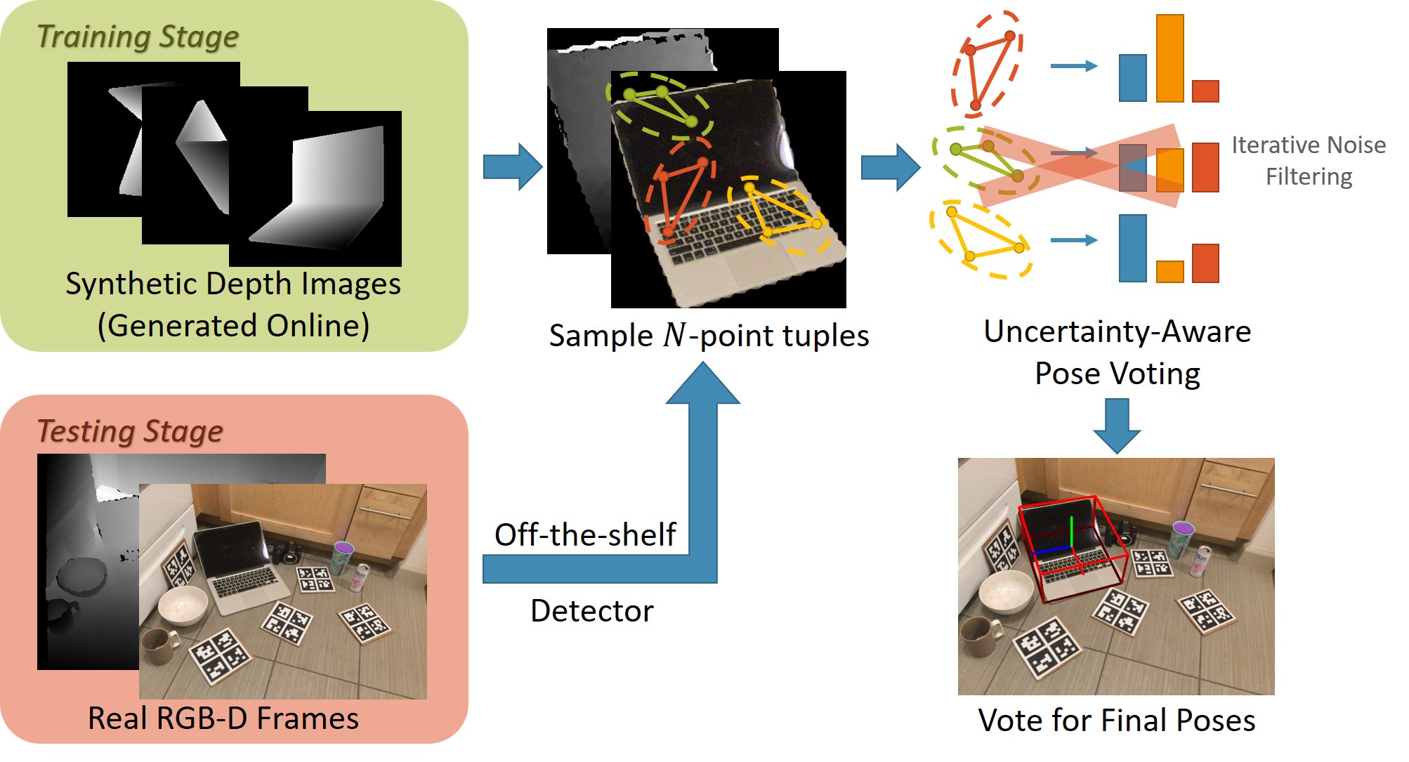
Figure 1: Unlike previous methods, our method leverages efficiently online-generated synthetic depth images for training. During inference, a collection of $N$-point tuples are uniformly sampled to vote poses with uncertainty awareness, culminating in the final prediction as the majority vote.

In this paper, we delve into the setting of efficient online synthetic training, wherein synthetic training data is generated on-the-fly. We contend that this setting is both practical and realistic, as it aligns with common scenarios where only a collection of scanned or synthetic CAD models are available, and rapid training of a pose detection model is desired without prior knowledge of potential backgrounds or clutters.

Building on the recent work of CPPF [39], which explored this problem setting and introduced a sim-to-real approach, we propose an enhanced voting method called CPPF++. Our method absorbs the voting scheme of CPPF but reformulates it from a probabilistic perspective. We model input point pairs as a multinomial distribution in the canonical space, sampling it to generate votes, and employ iterative noise filtering to mitigate background noise. Furthermore, we introduce $N$-point tuples to preserve more context information and present three rotation-invariant features to maintain rotation invariance.

To further evaluate the performance of current state-of-the-art methods, we introduce a more challenging category-level pose estimation dataset, DiversePose 300. This dataset overlaps with the NOCS REAL275 dataset but presents a significant drop in performance for existing methods, highlighting the effectiveness of our proposed method on this challenging dataset.

In summary, our contributions are three-fold:

• We approach the pose voting process from a probabilistic perspective, estimating the distribution of canonical coordinates of point pairs to manage uncertainty during voting. Iterative noise filtering and importance sample re-weighting techniques are deployed to effectively remove background noise or clutters.

• Our experiments demonstrate significant advancements over current synthetic methods on the NOCS REAL275 [36] dataset for category-level pose estimation and improvements over traditional PPF in instance-level pose estimation on the YCB-Video [38] dataset. To the best of our knowledge, our approach represents the pioneering effort in seamlessly integrating both instance-level and category-level pose estimation tasks, delivering commendable results.

• We introduce the DiversePose 300 dataset, a more challenging category-level pose dataset, to better evaluate current state-of-the-art methods. Our method exhibits superior performance on this dataset compared to previous methods, underscoring its efficacy and potential for further research and application.

2 Related Works

2.1 Pose Estimation Trained on Real-World Data

Currently, quite a lot of methods have been proposed for 6D pose estimation. For instance-level methods, PoseCNN [38] regresses the depth and 2D center offsets and a quaternion rotation for each region-of-interest with 2D CNNs. DeepIM [20] proposes to iteratively refine the initial pose estimation by giving a pose residual of comparing the rendered image and the input image. CosyPose [18] improves upon DeepIM by matching individual 6D object pose hypotheses across different images in order to jointly estimate camera viewpoints and 6D poses consistently. DenseFusion [34] learns a per-point confidence in RGB-D point clouds, and predicts the final pose with the best response. RCVPose [37] votes for keypoint locations by finding intersections of multiple spheres, and then use PnP to solve the final pose. In addition to instance-level methods, NOCS [36] first introduces a category-level pose estimation dataset and a regression method to learn the normalized coordinates of an object. CASS [3] proposes a variational auto-encoder to capture pose-independent features, along with pose dependent ones to predict 6D poses. DualPoseNet [22] uses two parallel decoders to make both an explicit and implicit representation of an object’s 6D pose. CenterSnap [15] represents object instances as center keypoints in a spatial 2D grid, and then regresses the object 6D pose at each position. ShAPO [16] improves CenterSnap by proposing a differentiable pipeline to improve the initial pose, along with the shape and appearance, using an octree structure. The above methods are mostly end-to-end and require real-world training data to work well.

2.2 Pose Estimation Trained on Synthetic Data

Fewer methods have been proposed to handle the problem of sim-to-real pose estimation. For instance-level pose estimation, Zhong et al. [42] develop a sim-to-real contrastive learning mechanism that can generalize the model trained in simulation to real-world applications. Likewise, TemplatePose [25] uses local feature encoder to compare the query image and the pre-rendered images from different views. It can be trained once and directly generalize to new objects. SurfEmb [10] learns dense and continuous 2D-3D correspondence distributions between the query image and the target model. It uses physical-based rendered training data provided by BOP challenge [14], which are generated offline. For category-level pose estimation, Chen et al. [5] propose to render synthetic models and compare the appearance with real images in different poses. Perhaps, CPPF [39] is the closest to this paper. It designs a special voting scheme by sampling numerous point pairs and predicting the voting targets. It is robust to noise and clutter and uses only the rendered synthetic object itself. However, its performance is still not as good as the current state-of-the-art, and it only conducts experiments on category-level pose estimation.

3 Method

In this section, we delineate the structure and key components of our proposed methodology. We commence by examining the most closely related work, CPPF, as detailed in Section 3.1. Subsequently, we provide a probabilistic perspective on our approach in Section 3.2.

Our work, denoted as CPPF++, is an extension of CPPF, and we introduce the following novel and critical strategies to enhance performance:

• Model Uncertainty Modeling: This strategy is elaborated in Section 3.3, where we discuss the incorporation of uncertainty into the model to improve robustness.

• Iterative Noise Filtering: In Section 3.4, we describe our approach to iterative noise filtering, a technique designed to refine the model’s predictions by reducing noise.

• N-Point Tuples: Section 3.5 is dedicated to our introduction of N-point tuples, a higher-order feature representation that captures more complex relationships within the data.

Furthermore, in Section 3.6, we discuss our method for predicting accurate category-level and instance-level masks in the absence of real-world training data. This innovation contributes to making our method a comprehensive sim-to-real pose estimation pipeline, without the necessity of incorporating any real-world training data.

Finally, Section 1 provides a detailed algorithmic description of our entire pipeline, encapsulating the aforementioned components and elucidating the cohesive functioning of our approach.

Together, these elements constitute a significant advancement in the field of object pose estimation, offering a robust and efficient methodology that is both theoretically sound and practically applicable.

3.1 Preliminaries: CPPF Voting

In the CPPF methodology, an established model for instance segmentation in images, such as MaskRCNN [11] or SAM [17], is initially utilized to delineate the object of interest. Upon obtaining the masked point cloud, denoted as $\mathbf{P}$, CPPF [39] selects $K$ point pairs from $\mathbf{P}$. For every point pair, CPPF derives rotation-invariant point pair features for input, subsequently forecasting several voting proxies that align with the object’s ground-truth center, orientation, and scale.

To elucidate further, let the object center be represented as $\mathbf{o}$. For each point pair, $\mathbf{p}_{1}$ and $\mathbf{p}_{2}$, CPPF estimates the subsequent two offsets:

$$\mu =(\mathbf{o}-\mathbf{p}_{1})\cdot\mathbf{d},$$ (1)

$$\nu =\|\mathbf{o}-(\mathbf{p}_{1}+\mu\mathbf{d})\|_{2},$$ (2)

where $$\mathbf{d}=\frac{\mathbf{p}_{2}-\mathbf{p}_{1}}{\|\mathbf{p}_{2}-\mathbf{p}_{1}\|_{2}},$$ (3)

as depicted in Figure 2(a). It is ensured that the ground-truth center resides on the sphere with its center at $\mathbf{c}$ and radius $\|\mathbf{o}-\mathbf{c}\|$. This voting target generation procedure will henceforth be referred to as:

$$(\mu,\nu)=g(\mathbf{o},\mathbf{p}_{1},\mathbf{p}_{2}).$$ (4)

During the inference phase, CPPF uniformly samples point pairs and subsequently enumerates votes around the circle. The predicted center, $\hat{\mathbf{o}}$, can be expressed as a function of the voting targets:

$$\hat{\mathbf{o}} =f(\hat{\mu},\hat{\nu},\hat{\sigma},\mathbf{p}_{1},\mathbf{p}_{2})$$ (5)

$$=\mathbf{p}_{1}+\hat{\mu}\mathbf{d}+\hat{\nu}(\cos(\sigma)\mathbf{d}_{\bot}+\sin(\sigma)\mathbf{d}\times\mathbf{d}_{\bot})$$ (6)

$$\text{where\quad}\mathbf{d}=\frac{\mathbf{p}_{2}-\mathbf{p}_{1}}{\|\mathbf{p}_{2}-\mathbf{p}_{1}\|_{2}},$$ (7)

where $\mathbf{d}_{\bot}$ represents an arbitrary unit vector orthogonal to $\mathbf{d}$, and $\hat{\sigma}$ is the sampled radial offset in the candidate circle, as illustrated by the red dashed circle in Figure 2(a). The location with the predominant vote is designated as the final center prediction.

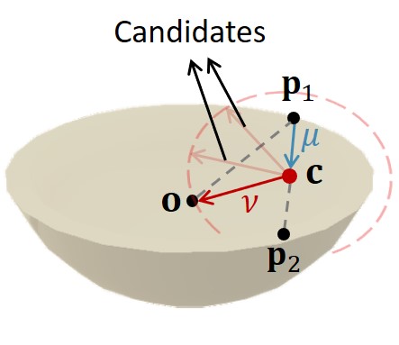
(a)

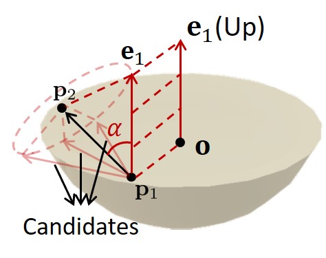
(b)

Figure 2: (a) Center voting mechanism of CPPF. Given a point pair $\mathbf{p}_{1},\mathbf{p}_{2}$, CPPF predicts $\mu$ and $\nu$, with $\mathbf{c}$ representing the perpendicular foot. (b) Orientation voting mechanism of CPPF. For each point pair, CPPF estimates the angle $\alpha$ between $\mathbf{p}_{2}-\mathbf{p}_{1}$ and $\mathbf{e}_{1}$.

Regarding orientation voting, CPPF casts votes for the object’s upward and rightward orientation basis. The remaining basis is derived using a cross product. With the upward orientation symbolized as $\mathbf{e}_{1}$ and the rightward orientation as $\mathbf{e}_{2}$, CPPF predicts the subsequent two relative angles:

$$\alpha =\mathbf{e}_{1}\cdot\frac{\mathbf{p}_{2}-\mathbf{p}_{1}}{\|\mathbf{p}_{2}-\mathbf{p}_{1}\|_{2}}$$ (8)

$$\beta =\mathbf{e}_{2}\cdot\frac{\mathbf{p}_{2}-\mathbf{p}_{1}}{\|\mathbf{p}_{2}-\mathbf{p}_{1}\|_{2}},$$ (9)

as illustrated in Figure 2(b). Analogous to the center voting mechanism, CPPF enumerates votes around the red dashed cone, and the orientation amassing the highest number of votes is selected as the final prediction.

For scale prediction, CPPF estimates the scale, denoted as $\mathbf{s}$, for each point pair and subsequently computes their average during the inference phase.

3.2 A Probabilistic View of Point Pair Voting

CPPF formulates rotation-invariant voting proxies, casting votes for a prospective center, orientation, and scale for each point pair. Without compromising generality, during center voting and given the point pair $\mathbf{p}_{1},\mathbf{p}_{2}$, the ground-truth object center, denoted as $\mathbf{o}$, is unequivocally determined by parameters $\mu,\nu,\sigma$ through the function $f(\mu,\nu,\sigma,\mathbf{p}_{1},\mathbf{p}_{2})$. Here, $\mu$ and $\nu$ are the proxies delineated in Equations 1 and 2, respectively, while $\sigma$ represents the ground-truth radial angle offset on the sphere centered at $\mathbf{c}$ with a radius of $|\mathbf{o}-\mathbf{c}|$. Note that CPPF does not directly predict $\sigma$ but samples it uniformly during the inference phase.

Examining this from a probabilistic perspective, the voting procedure endeavors to optimize the probability of the predicted center, $\hat{\mathbf{o}}$:

$$p(\hat{\mathbf{o}})=\int \delta(\hat{\mathbf{o}}-f(\mu,\nu,\sigma,\mathbf{p}_{1},\mathbf{p}_{2}))p(\mu,\nu,\sigma|\mathbf{p}_{1},\mathbf{p}_{2})$$ (10)

$$\cdot p(\mathbf{p}_{1},\mathbf{p}_{2})d\mathbf{p}_{1}d\mathbf{p}_{2}.$$ (11)

Here, $\delta$ denotes the Dirac delta function. Introducing a naive Bayes prior, under the assumption that $\mu,\nu$, and $\sigma$ are conditionally independent, Equation 11 can be reformulated as:

$$p(\hat{\mathbf{o}})=\int \underbrace{\delta(\hat{\mathbf{o}}-f(\mu,\nu,\sigma,\mathbf{p}_{1},\mathbf{p}_{2}))}_{\textrm{ \leavevmode\hbox to11.75pt{\vbox to11.75pt{\text{[drawing]}}}}}\underbrace{p(\mu,\nu|\mathbf{p}_{1},\mathbf{p}_{2}))}_{\textrm{ \leavevmode\hbox to11.75pt{\vbox to11.75pt{\text{[drawing]}}}}}\underbrace{p(\sigma|\mathbf{p}_{1},\mathbf{p}_{2})}_{\textrm{ \leavevmode\hbox to11.75pt{\vbox to11.75pt{\text{[drawing]}}}}}$$ (12)

$$\cdot\underbrace{p(\mathbf{p}_{1},\mathbf{p}_{2})d\mathbf{p}_{1}d\mathbf{p}_{2}}_{\textrm{ \leavevmode\hbox to11.75pt{\vbox to11.75pt{\text{[drawing]}}}}}.$$ (13)

This equation elucidates the operations of CPPF’s voting mechanism: for each sampled point pair $\mathbf{p}_{1},\mathbf{p}_{2}$, the system predicts $\mu,\nu$ utilizing a neural network, and uniformly samples $\sigma$, operating under the assumption that $\sigma$ is independent of $\mathbf{p}_{1},\mathbf{p}_{2}$ (i.e., $p(\sigma|\mathbf{p}_{1},\mathbf{p}_{2})=p(\sigma)$). Subsequently, the definitive center is determined by $f(\mu,\nu,\sigma,\mathbf{p}_{1},\mathbf{p}_{2})$, as illustrated in Figure 2(a).

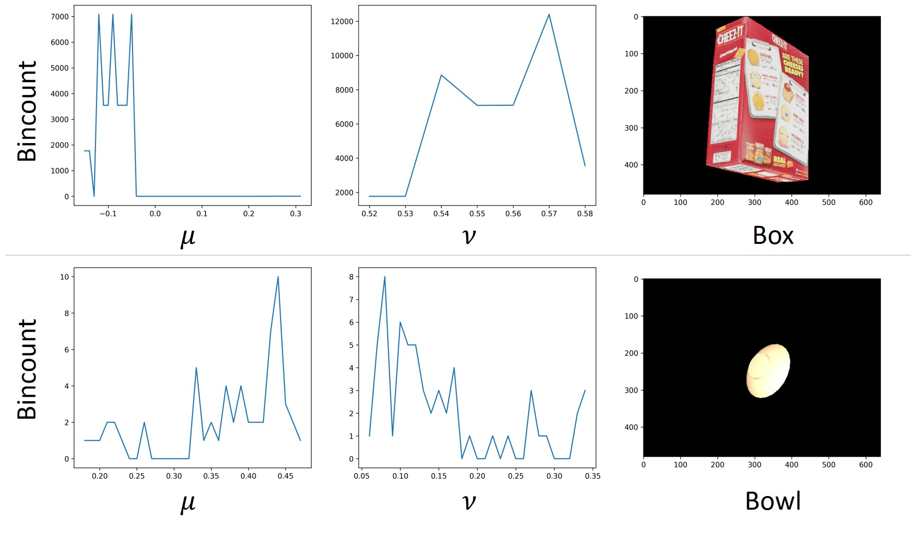
Figure 3: This figure provides a visual representation of voting collision for two objects: a box and a bowl. For each object, the initial step involves hashing all input point pair features, followed by counting the voting targets $\mu,\nu$ for the input point pairs in the most populated hash bin. It becomes evident that analogous input point pair features yield considerably divergent voting targets, rendering it challenging to discern a consistent deterministic relationship between the input and output.

3.3 Vote Uncertainty Modeling

Predicting $\mu,\nu$ directly as scalars from $\mathbf{p}_{1},\mathbf{p}_{2}$ presents challenges due to the potential for similar input point pairs to yield divergent $\mu,\nu$ values, a phenomenon termed ”voting collision.” As illustrated in Figure 3, for numerous prevalent objects, the voting collision ratio is significantly large and warrants attention. Consequently, our approach aims to explicitly model this uncertainty by introducing a canonical space decomposition of $p(\mu,\nu|\mathbf{p}_{1},\mathbf{p}_{2})$:

$$p(\mu,\nu|\mathbf{p}_{1},\mathbf{p}_{2})=\delta((\mu,\nu)-g(\bar{\mathbf{o}},\bar{\mathbf{p}}_{1},\bar{\mathbf{p}}_{2}))p(\bar{\mathbf{p}}_{1},\bar{\mathbf{p}}_{2}|\mathbf{p}_{1},\mathbf{p}_{2}),$$ (14)

where $g(\cdot)$ is defined in Equation 4, and $\bar{\mathbf{p}}_{1},\bar{\mathbf{p}}_{2}$ are the canonical coordinates of $\mathbf{p}_{1},\mathbf{p}_{2}$. Suppose the ground-truth rotation and translation are $\mathbf{R}$ and $\mathbf{t}$, then $\mathbf{R}\cdot\bar{\mathbf{p}}_{1}+\mathbf{t}=\mathbf{p}_{1}$ and $\mathbf{R}\cdot\bar{\mathbf{p}}_{2}+\mathbf{t}=\mathbf{p}_{2}$ hold true.

Equation 14 intuitively captures uncertainty by representing the distribution of canonical point pairs to which $\mathbf{p}_{1},\mathbf{p}_{2}$ correspond. Practically, we interpret $p(\bar{\mathbf{p}}_{1},\bar{\mathbf{p}}_{2}|\mathbf{p}_{1},\mathbf{p}_{2})$ as a multinomial distribution over discretized 3D grids within the canonical space. Upon determining the canonical coordinates $\bar{\mathbf{p}}_{1},\bar{\mathbf{p}}_{2}$, we can derive $\mu,\nu$ using $g(\bar{\mathbf{o}},\bar{\mathbf{p}}_{1},\bar{\mathbf{p}}_{2}))$. This is feasible since the ground-truth center $\bar{\mathbf{o}}$ of the canonical mesh is consistently $(0,0,0)$, and both $\mu$ and $\nu$ remain invariant to $SE(3)$ transformations.

In the context of orientation voting, we decompose $p(\alpha,\theta|\mathbf{p}_{1},\mathbf{p}_{2})$ into $\delta((\alpha,\theta)-g(\mathbf{e}_{1},\bar{\mathbf{p}}_{1},\bar{\mathbf{p}}_{2}))p(\bar{\mathbf{p}}_{1},\bar{\mathbf{p}}_{2}|\mathbf{p}_{1},\mathbf{p}_{2})$. Here, $\alpha$ is the target as defined in Equation 8, while $\theta$ represents the residual radial degree of freedom, as illustrated in Figure 2(b). As our experimental results will demonstrate, this uncertainty modeling significantly enhances performance, rendering the voting procedure more precise.

Regarding scale voting, given that a singular global scaling applies to all point pairs, we adopt the CPPF methodology, predicting the scale $s$ for each point pair and subsequently computing their average during the inference phase.

3.4 Iterative Noise Filtering

In practical applications, object segmentation often falls short of perfection, potentially including background noise or occlusions that require filtering. Such imperfections significantly undermine the efficacy of orientation voting. To mitigate this, we incorporate a noise filtering module, utilizing the current object center estimate for reference.

To identify and exclude unreliable point pairs, we compute the error of $\mu,\nu$ for each point pair based on the current estimate:

$$\epsilon=\|g(\hat{\mathbf{o}},\mathbf{p}_{1},\mathbf{p}_{2}))-g(\bar{\mathbf{o}},\bar{\mathbf{p}}_{1},\bar{\mathbf{p}}_{2}))\|_{2}.$$ (15)

Here, $\hat{\mathbf{o}}$ represents the majority’s predicted center, while $\bar{\mathbf{o}}$ is fixed at $(0,0,0)$. For the sampled point pairs $\mathbf{p}_{1}^{(k)},\mathbf{p}_{2}^{(k)}$, where $k$ signifies the sample index, we compute all corresponding errors $\epsilon^{(k)}$. Point pairs with errors in the top $\tau\times 100\%$ are subsequently discarded. Although this consistency verification can be executed iteratively by updating $\hat{\mathbf{o}}$, empirical observations indicate that a singular iteration suffices to eliminate the majority of noise. Adopting this approach significantly bolsters the precision of orientation voting, ensuring a more robust voting mechanism.

3.4.1 Importance Sample Re-weighting

While the original point pairs are uniformly sampled from the point cloud, the iterative noise filtering process can disrupt this balance. As a result, certain points may be assigned reduced weights, especially if a significant number of point pairs linked to them are filtered out. In the subsequent phase, operating under the premise that each point should have an equal influence on the final voting outcome, we adjust the weight of each point inversely based on the number of point pair samples connected to it. While one could opt to re-sample the point pairs from the filtered point clouds, this approach incurs additional computational costs, as the newly sampled point pair input features would need to be reprocessed through our network to determine the output voting targets.

To clarify, when we discuss re-weighting a point, we refer to the process wherein all votes produced by point pairs that include this specific point are adjusted by the weights during the majority tally. This process is analogous to employing a weighted probability for point pair samples, represented as $p(\mathbf{p}_{1},\mathbf{p}_{2})w(\mathbf{p}_{1})w(\mathbf{p}_{2})$, where $w(\mathbf{p}_{1})$ and $w(\mathbf{p}_{2})$ denote the re-weighting factors:

$$w(\mathbf{p}_{1}) =\frac{1}{|\{\mathbf{p}_{1},\mathbf{p}_{2}^{\prime}|\mathbf{p}_{2}^{\prime}\in\mathbf{P}\}|+\eta}$$ (16)

$$w(\mathbf{p}_{2}) =\frac{1}{|\{\mathbf{p}_{1}^{\prime},\mathbf{p}_{2}|\mathbf{p}_{1}^{\prime}\in\mathbf{P}\}|+\eta}.$$ (17)

The notation $|\cdot|$ represents the cardinality of a set, while $\eta$ serves as a margin value, introduced to stabilize the denominator in instances where it encounters small numbers. An illustrative example is provided in Figure 4: prior to noise filtering, all point pairs are assigned relatively uniform weights, and some background noise is evident. Following the noise filtering process, a significant portion of this noise is eradicated. However, certain regions of the mug receive fewer samples compared to others. This distribution is not ideal, as ideally, each point should have an approximately equal influence on the final pose determination.

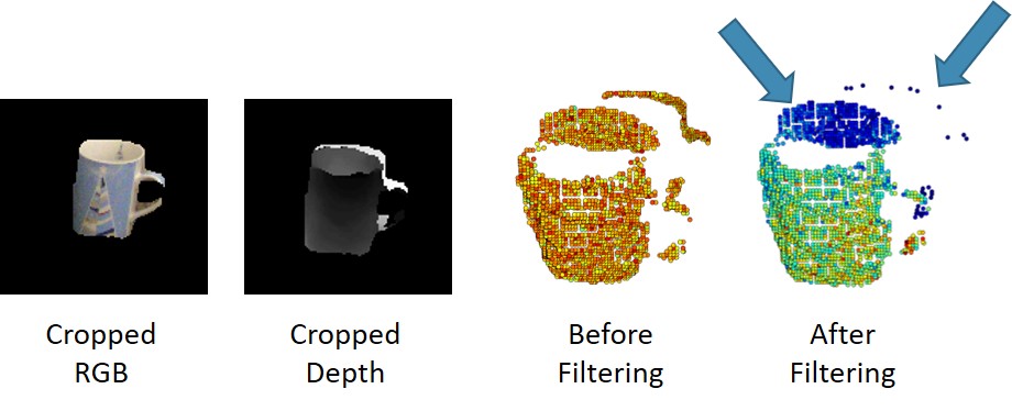
Figure 4: Illustration of Iterative Noise Filtering and Importance Re-weighting. Given the detection outcome, background noise may be present, attributable to depth sensor inaccuracies or suboptimal segmentation. On the right, the average sample counts for each point, both pre and post noise filtering, are depicted: red signifies high counts, and blue denotes low. It is evident that the filtering algorithm effectively mitigates the majority of noise but concurrently introduces sampling imbalances on the mug. To maintain uniform sampling, we adjust the weight of each sample inversely based on their counts, obviating the need for re-sampling.

3.5 $N$-Point Tuples

CPPF’s input features and output voting targets exhibit invariance to arbitrary translations and rotations, making its voting mechanism readily adaptable to real-world contexts. Nevertheless, we observed that the point pair features delineated in CPPF lack enough context required to differentiate between various voting outputs. To mitigate voting collision, we have expanded the rudimentary point pair features to encompass $N$-point tuple features.

To elaborate, we commence by sampling $K$ $N$-point tuples from the object. For each tuple, denoted as $\mathcal{T}=\{\mathbf{p}_{1},\mathbf{p}_{2},\cdots,\mathbf{p}_{N}\}$, we calculate both the normal and local SHOT [28] descriptors for every point. These are represented as $\{\mathbf{n}_{1},\mathbf{n}_{2},\cdots,\mathbf{n}_{N}\}$ and $\{\psi_{1},\psi_{2},\cdots,\psi_{N}\}$, respectively. For each $N$-point tuple, we employ the subsequent three features as input to our network:

$$\mathcal{F}_{1} =\mathbf{concat}(\{\mathbf{p}_{i}-\mathbf{p}_{j}|(i,j)\in\sigma^{2}(N)\})$$ (18)

$$\mathcal{F}_{2} =\mathbf{concat}(\{\max(\mathbf{n}_{i}\cdot\mathbf{n}_{j},-\mathbf{n}_{i}\cdot\mathbf{n}_{j})|(i,j)\in\sigma^{2}(N)\})$$ (19)

$$\mathcal{F}_{3} =\mathbf{concat}(\{\mathrm{MLP}(\psi_{i})|i=1,2,3,\cdots,N\}),$$ (20)

where $\sigma^{2}(N)$ denotes all combinations of order 2 from $N$ (commonly referred to as ”$N$ choose 2”), $\mathbf{concat}$ signifies concatenation, and MLP layers are employed to encode SHOT descriptors into concise embeddings. Feature $\mathcal{F}_{1}$ encompasses relative coordinates, $\mathcal{F}_{2}$ integrates relative normal angles, and $\mathcal{F}_{3}$ captures the local context surrounding each point. It’s imperative to note that all three features exhibit translation invariance. Furthermore, both $\mathcal{F}_{2}$ and $\mathcal{F}_{3}$ are rotation invariant. In practical applications, employing a straightforward rotation augmentation ensures that $\mathcal{F}_{1}$ also achieves rotation invariance.

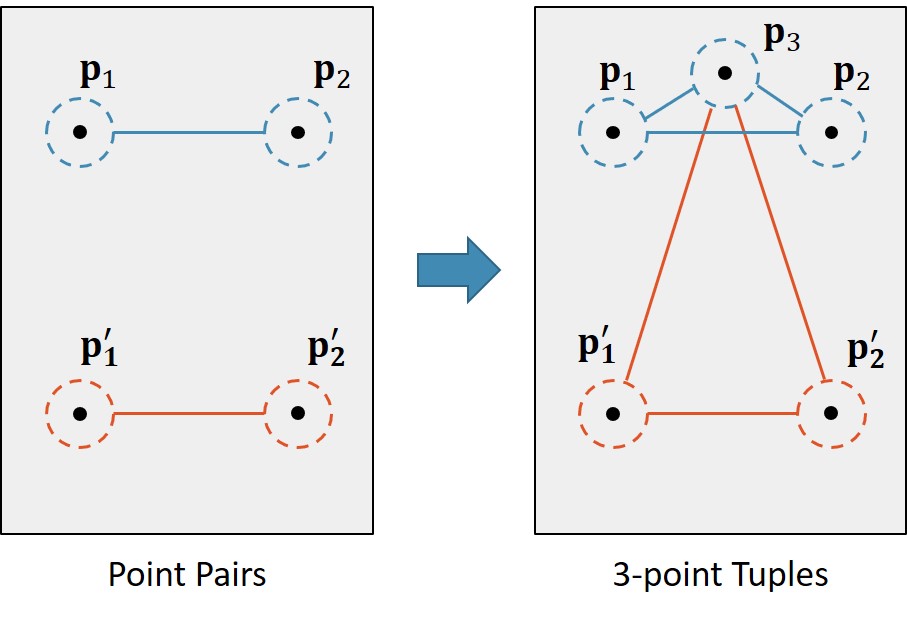
Figure 5: Contrast between Point Pairs and $N$-point Tuples. The dashed circle represents the local context surrounding each point. Left: The two point pairs, $\mathbf{p}_{1},\mathbf{p}_{2}$ and $\mathbf{p}^{\prime}_{1},\mathbf{p}^{\prime}_{2}$, possess identical relative coordinates and local contexts, rendering them indiscernible. Right: Conversely, by introducing an extra point, $\mathbf{p}_{3}$, and creating 3-point tuples using the initial point pairs, the resulting 3-point tuples can now be differentiated based on their relative coordinates.

To elucidate why $N$-point tuples offer more comprehensive information compared to basic point pairs, we present a succinct example in Figure 5. On the left side of the figure, two point pairs appear identical when assessed based on their relative coordinates. Distinguishing between these two pairs becomes unfeasible without the inclusion of additional points. However, by introducing another point, say $\mathbf{p}_{3}$, and constructing 3-point tuples for each original point pair, differentiation becomes possible by calculating the relative coordinates in relation to this supplementary point.

3.6 Instance Mask Prediction

A salient advantage of our method lies in its reliance solely on synthetic depth images rendered with CAD models during the training phase. However, our approach does necessitate instance segmentation to sample point tuples on objects, and the instance segmentation module may require additional real-world RGB training data to function optimally.

Fortunately, recent advancements in zero-shot segmentation methods, such as SAM [17] and Grounded DINO [23], have demonstrated promising performance in real-world scenarios. In this section, we elucidate how to obtain reliable instance segmentation without the need for additional real-world training data, thereby transforming our method into a comprehensive sim-to-real pipeline.

For category-level detection, we employ Grounded FastSAM [23, 40], utilizing the text description for each category as the prompt (e.g., bowl, mug, bottle, etc.). The scenario becomes more intricate for instance-level detection, where both the CAD model and text description of the target object are known a priori. In our experiments on the YCB-Video dataset, we observed that the text description of each instance does not consistently facilitate the retrieval of the target instance. Consequently, we propose a two-stage one-shot detection algorithm:

• First Stage: This stage aims to recall all potential target objects by employing the union of the text prompts from all instances, with Grounded FastSAM [23, 40].

• Second Stage: Here, we fine-tune the CLIP model [26] using our synthetically rendered RGB images to classify each crop into distinct instances.

In the interest of a fair comparison, our experimental results include both the outcomes obtained with a commonly used pre-trained instance detector (aligned with previous methods) and those achieved with zero-shot/one-shot instance segmentation methods. This dual reporting underscores the flexibility and robustness of our approach, highlighting its potential for broader application in object pose estimation tasks.

3.7 Algorithm Summary

In this section, we give a detailed description of our pipeline in Algorithm 1.

1:: RGB-D image

2:: Pose estimations for all the objects

3:Get candidate instance segmentations $\{S_{i}\}$ using off-the-shelf methods

4:for each $S_{i}\in\{S_{i}\}$ do

5:     Crop the depth image and back-project into point cloud

6:     for each sampled $N$-point tuple $\mathcal{T}$ from point cloud do

7:         Construct feature $\mathcal{F}_{1},\mathcal{F}_{2},\mathcal{F}_{3}$

8:         Forward the features to the MLP network, and get the output distribution of $\bar{\mathbf{p}}_{1},\bar{\mathbf{p}}_{2}$.

9:         Sample from the distribution, and calculate $(\mu,\nu)=g(\bar{\mathbf{o}},\bar{\mathbf{p}}_{1},\bar{\mathbf{p}}_{2}))$

10:         Vote for the center $\hat{\mathbf{o}}$ using $\mu,\nu$

11:         Do iterative noise filtering and remove noisy tuples

12:         Calculate $(\alpha,\beta)$ with the remaining tuples

13:         Vote for the orientation axis $\mathbf{e}_{1},\mathbf{e}_{2}$ using $\alpha,\beta$ with vote re-weighting

14:         Construct rotation matrix $\hat{\mathbf{R}}=[\mathbf{e}_{1};\mathbf{e}_{2};\mathbf{e}_{1}\times\mathbf{e}_{2}]$

15:         Average over the predicted scale for each tuple to get the scale prediction $\hat{\mathbf{s}}$

16:         Output pose $\{\hat{\mathbf{R}},\hat{\mathbf{o}},\hat{\mathbf{s}}\}$ for current segmentation

17:     end for

18:end for

Algorithm 1 Inference Stage of CPPF++

4 DiversePose 300: A New Dataset with Diverse Poses and Clutters

The DiversePose 300 dataset represents a novel contribution to the field of object pose estimation, encompassing three common object categories: bowls, bottles, and mugs. Each category is represented by 100 annotated frames, resulting in a total of 300 distinct frames. This contrasts sharply with the NOCS REAL275 dataset, which consists of only 6 continuous videos for evaluation.

The DiversePose 300 dataset is meticulously designed to enhance pose diversity by ensuring that each annotated frame is independent of the others. This design choice significantly differentiates it from continuous video datasets and contributes to its complexity. The dataset is further subdivided into three scenarios, each representing a different level of difficulty:

• Easy: A single object is placed on the desktop with a relatively clean background.

• Medium: A single object is held by hand, with a relatively clean background.

• Hard: Multiple objects are scattered on the material box or desktop, and the background is relatively complex.

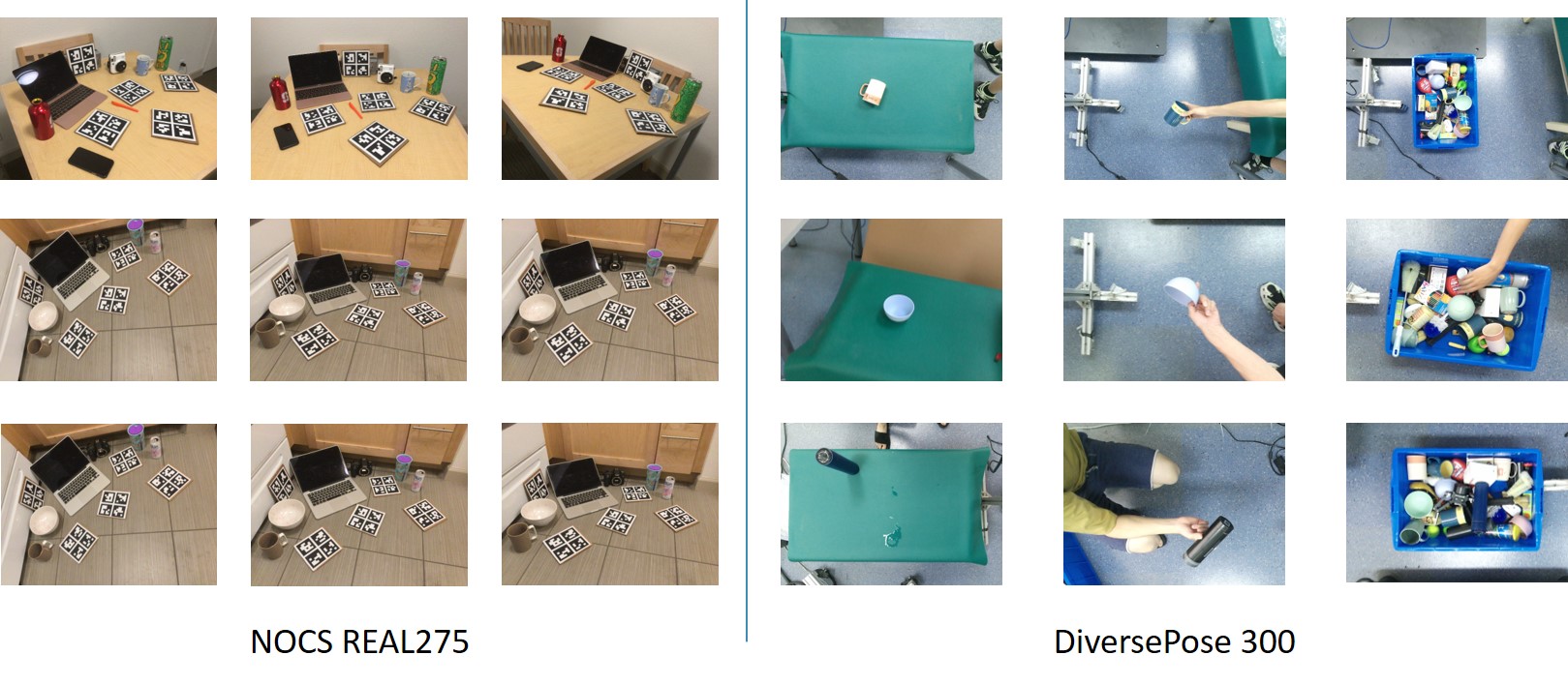
Figure 6: A qualitative comparison between our NOCS REAL275 and DiversePose 300. NOCS REAL275 is biased towards similar backgrounds and upright poses, while DiversePose 300 captures pose variation under different backgrounds and difficulties.

A qualitative comparison between DiversePose 300 and NOCS REAL275 (illustrated in Figure 6) reveals significant differences in complexity and diversity.

Despite its modest size, DiversePose 300 presents a substantial challenge to current state-of-the-art methods, with performance far from saturation. This underscores the dataset’s potential as a rigorous benchmark for evaluating pose estimation algorithms.

The distinctions between DiversePose 300 and NOCS REAL275 can be summarized in three key aspects:

• Annotation Diversity: Unlike the continuous videos in NOCS REAL275, DiversePose 300’s individual unrelated frames result in more diverse pose annotations.

• Robustness of Evaluation: The inclusion of challenging scenarios such as bin clutters and hand manipulation emphasizes the evaluation of algorithm robustness.

• Depth Rendering Complexity: The utilization of the Intel RealSense camera, as opposed to the Structure Sensor used in NOCS REAL275, creates more challenging depth renderings, necessitating that evaluated methods generalize across different data domains.

In conclusion, DiversePose 300 offers a unique and challenging dataset that advances the field of object pose estimation. Its design emphasizes diversity, complexity, and robustness, setting it apart from existing datasets such as NOCS REAL275 and positioning it as a valuable resource for researchers and practitioners alike.

5 Implementation Details

In our approach, we opt for $5$-point tuples and set a filtering ratio of $\tau=0.5$, with re-weighting margin $\eta=1.0$. Within our model, each $5$-point tuple is processed independently to predict a voting proxy, and the network architecture is composed of several distinct components: a SHOT feature encoder, a tuple encoder, a logit encoder, and a scale encoder.

• SHOT Feature Encoder: This encoder is responsible for compactly embedding each point’s SHOT descriptor. It consists of five residual MLP layers, following the architecture proposed by He et al. [12].

• Tuple Encoder: Comprising $128\times 5$ hidden residual MLP layers, the tuple encoder culminates in a final layer with $256$ neurons. Subsequently, either the logit encoder or the scale encoder is concatenated to this structure.

• Logit Encoder: This encoder features two hidden layers and produces $2\times 3\times 32$ outputs, representing the distribution of the canonical coordinate for each point pair. The distribution is discretized into 32 bins across the three $xyz$ axes.

• Scale Encoder: Comprising two hidden layers with $256$ and $128$ neurons, the scale encoder ultimately yields three outputs, predicting the $xyz$ scale for each tuple.

Training is conducted separately for each category or instance, utilizing the Adam optimizer with a learning rate of $1\times 10^{-3}$. The training process spans 100 epochs, with the learning rate being halved every 25 epochs.

During the training stage, to emulate self-occlusions, we adhere to the method employed by CPPF, leveraging Pyrender with an OpenGL back-end [24] to synthesize projected point clouds online. Our method utilizes the identical synthetic ShapeNet objects as CPPF [2]. At the inference stage, our network directly accepts the depth image segmentation as input.

In the center voting process, the accumulation 3D grid is defined with a resolution of 0.2 cm, and its range is determined by the tightest axis-aligned bounding box of the input. During the orientation voting process, the orientation grid is set with a resolution of 1 degree, ensuring precision in the pose estimation.

6 Experiments

6.1 Results on NOCS REAL275

6.1.1 Datasets.

NOCS REAL275 [36] dataset is a common benchmark used to evaluate our method on category-level pose estimation, where only a collection of similar objects in the same category during training time. NOCS REAL275 dataset captures 2750 test frames of 6 real scenes using a Structure Sensor.

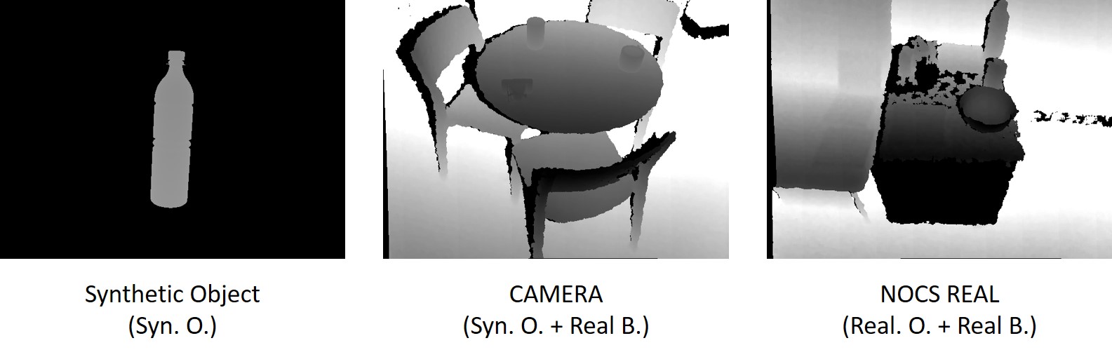
Figure 7: Visualization of different training data modalities. Our method uses synthetic objects (Syn. O.) where no background or clutter prior is introduced; CAMERA (Syn. O. + Real B.) composes images by placing rendered synthetic objects on real backgrounds (i.e., tables); NOCS REAL (Real O. + Real B.) is a dataset captured with real objects placed in real scenarios.

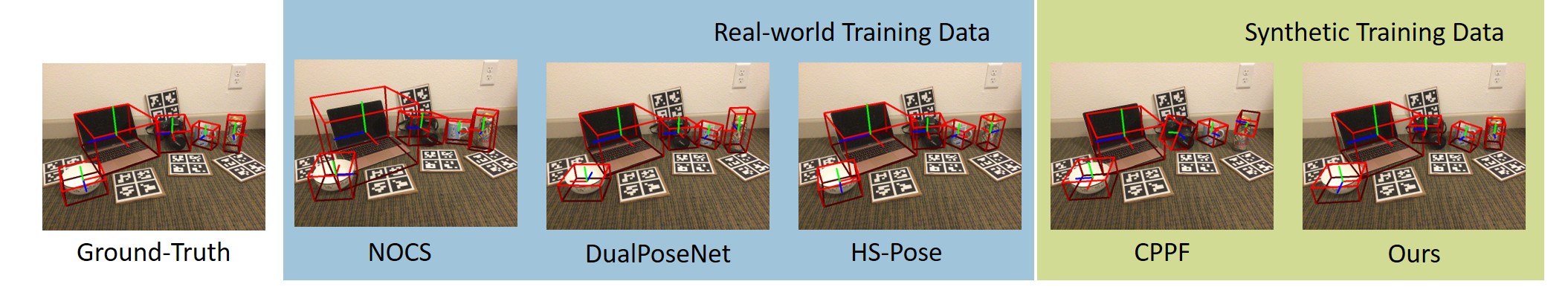
Figure 8: Comparison of different methods on NOCS REAL275 dataset. Though trained with synthetic CAD models, our method is comparable to current state-of-the-arts.

6.1.2 Metrics.

We adopt the metrics from NOCS [36] to present results using both intersection over union (IoU) and 6D pose average precision. The IoU is determined by comparing the predicted bounding boxes with the ground-truth, using thresholds of 25% and 50%. Meanwhile, the 6D pose average precision is ascertained by gauging the average precision for objects where the error is below $m$ cm for translation and $n^{\circ}$ for rotation.

It is noteworthy that the original code for 3D box mAP computation provided by NOCS contains errors. Consequently, we, in alignment with CPPF, have opted to utilize the code available in Objectron [1]. This flawed code has been inadvertently adopted by numerous subsequent studies. As a result, we have taken the initiative to reproduce the results for 3D box mAP specifically for NOCS, DualPoseNet, and HS-Pose, given that they offer reproducible code.

6.1.3 Baselines.

Based on the modality of the training data utilized, we categorize the baselines into three distinct types. SAR-Net [21] employs the CAMERA synthetic dataset provided by NOCS, wherein synthetic CAD models are superimposed onto real background tables. SAR-Net is heavily dependent on this background prior to filter out noise from the instance mask. Methods such as NOCS [36], CASS [3], SPD [32], FS-Net [4], CenterSnap [15], ShAPO [16], DualPoseNet [22], and HS-Pose [41] utilize both the CAMERA synthetic dataset and the real training set offered by NOCS. Chen et al. [5], Gao et al. [9], and CPPF [39] exclusively use synthetic objects, devoid of any background simulation. Our approach aligns with CPPF in using synthetic objects. The distinctions among the Synthetic Object, CAMERA, and NOCS REAL datasets are depicted in Figure 7. Given that the provided mask/detection prior often includes noise or background elements, the task of sim-to-real transfer becomes inherently challenging.

For a fair comparison, all methods utilize the mask prior provided by NOCS, with the exception of DualPoseNet, CenterSnap, and ShaPO. These particular methods train their own masks, which tend to be marginally superior to those furnished by NOCS, potentially rendering their results more favorable.

6.1.4 Results.

	Training Data	mAP (%)
		3D25	3D50	5∘ 5 cm	10∘ 5 cm	15∘ 5 cm
NOCS [36]	Syn. O. + Real O. & B.	74.4	27.8	9.8	24.1	34.9
CASS [3]	Syn. O. + Real O. & B.	-	-	23.5	58.0	-
SPD [32]	Syn. O. + Real O. & B.	-	-	21.4	54.1	-
FS-Net [4]	Syn. O. + Real O. & B.	-	-	28.2	60.8	-
CenterSnap [15]	Syn. O. + Real O. & B.	-	-	27.2	58.8	-
ShAPO [16]	Syn. O. + Real O. & B.	-	-	48.8	66.8	-
DualPoseNet [22]	Syn. O. + Real O. & B.	82.3	57.3	36.1	67.8	76.3
HS-Pose [41]	Syn. O. + Real O. & B.	82.6	71.6	56.1	84.1	92.8
SAR-Net [21]	Syn. O. + Real B.	-	-	42.3	68.3	-
Chen et al. [5]	Syn. O.	15.5	1.3	0.7	3.6	9.1
Gao et al. [9]	Syn. O.	68.6	24.7	7.8	17.1	26.5
CPPF [39]	Syn. O.	78.2	26.4	16.9	44.9	50.8
Ours	Syn. O.	71.7	40.1	22.1	64.0	71.7
Ours w/ GroundedSAM Det.	Syn. O.	64.6	38.4	28.8	64.5	74.2

TABLE I: Comparison of various methods on NOCS REAL275. The best methods that use real training data and synthetic data are bolded respectively.

Quantitative outcomes are presented in Table I. It is evident that our approach significantly surpasses CPPF across nearly all metrics, registering improvements of 14.3, 5.2, 19.1, and 20.9 in terms of 3D₅₀, 5^∘5 cm, 10^∘5 cm, and 15^∘5 cm, respectively. Our method also holds its own against numerous techniques that employ real training data. While HS-Pose exhibits commendable performance on NOCS REAL275, as we will discuss in Section 6.2, its efficacy considerably diminishes on the DiversePose 300 dataset. Additionally, we present pose estimation results utilizing GroundedSAM [23, 17] as our detector, which further enhances performance by delivering marginally improved segmentation. CPPF++ effectively bridges the domain gap between sim-to-real and methods trained on real data. Visual comparisons are showcased in Figure 8.

	mAP (%)
	3D25	3D50	5∘ 5 cm	10∘ 5 cm	15∘ 5 cm
Bottle	23.7	0.0	28.7	93.5	97.2
Bowl	100.0	93.8	31.5	88.9	97.9
Camera	62.8	0.1	0.0	0.1	0.3
Can	50.8	9.6	31.6	82.7	88.1
Laptop	99.6	91.3	39.4	90.6	91.0
Mug	93.1	45.6	1.6	28.5	55.7

TABLE II: Per-category performance of the proposed method on NOCS REAL275.

6.1.5 Detailed Analysis and Failure Cases.

Detailed per-category outcomes are provided in Table II. The subpar performance associated with the camera category can be attributed to the disparity between synthetic CAD models and actual objects. As illustrated in Figure 9, the CAD models under evaluation and the synthetic CAD models for cameras belong to distinct types. This variance cannot be rectified without employing real-world training data that aligns with the same distribution.

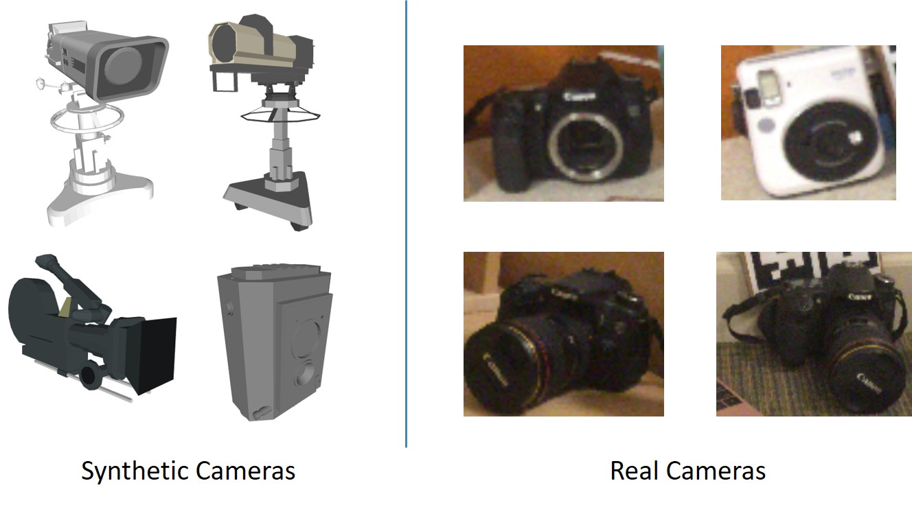
Figure 9: In NOCS REAL275 dataset, there is a distribution shift between synthetic and real cameras, causing a drop of our method on the camera category.

6.2 Results on DiversePose 300

Though current state-of-the-art methods get decent results on NOCS REAL275, we are extremely interested in if these methods can generalize to other data distributions. As a result, we collect DiversePose 300, a much more challenging and diverse category-level pose evaluation dataset.

6.2.1 Datasets.

The DiversePose 300 dataset represents a novel contribution to the field of object pose estimation, encompassing three common object categories: bowls, bottles, and mugs. Each category is represented by 100 annotated frames, resulting in a total of 300 distinct frames.

6.2.2 Metrics.

We use exactly the same metric as NOCS REAL275, while loosen the AP threshold to $20^{\circ},40^{\circ},60^{\circ}$ since this is a challenging benchmark.

6.2.3 Baselines.

We have selected four representative baseline methods for comparative analysis: NOCS [36] (the pioneering category-level pose estimation method), DualPoseNet [22] (the state-of-the-art prior to 2022), HS-Pose [41] (the state-of-the-art post-2022), and CPPF [39] (a purely sim-to-real approach).

To ensure an equitable comparison, we retrained all the methods incorporating rotation augmentation that covers the entire $SO(3)$ space. The training dataset comprises synthetically rendered RGB-D frames with randomized orientations and translations of objects. We also assessed the pre-trained models of baselines that were trained on NOCS real-world data, only to find their performance even worse. During the inference phase, all methods employ the mask prior derived from the leading-edge detector, Masked-DINO [19].

6.2.4 Results.

As delineated in Table III, our introduced method markedly surpasses preceding methodologies on this demanding dataset across all three categories. Baseline methods get struggled with the diverse poses and backgrounds present in DiversePose 300. They exhibit a propensity to skew towards the distribution of their training data, whereas our model demonstrates robustness in generalizing to previously unseen data. While CPPF manages to produce some plausible results, it remains subpar compared to our proposed approach. A visual comparison is presented in Figure 10.

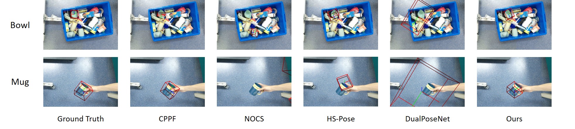
Figure 10: Qualitative comparison of different methods on DiversePose 300. When transferring to a new data domain, our method shows strong generalizability than previous methods.

		IoU (%)$\uparrow$		AP (%)$\uparrow$
		3D25	3D50	20∘ 5 cm	40∘ 5 cm	60∘ 5 cm
NOCS [36]	mug	4.9	2.4	0.0	1.7	1.9
	bowl	1.7	0.3	0.5	0.5	0.5
	bottle	3.3	0.0	2.3	2.3	2.3
DualPoseNet [22]	mug	0.0	0.0	0.1	0.1	0.1
	bowl	0.3	0.0	0.0	0.0	0.2
	bottle	0.0	0.0	0.0	0.0	0.0
HS-Pose [41]	mug	8.3	0.1	0.0	0.6	0.8
	bowl	11.2	0.0	1.4	10.5	17.3
	bottle	0.2	0.0	0.5	10.5	15.1
CPPF [39]	mug	35.8	15.2	0.7	1.0	2.3
	bowl	32.7	3.4	14.5	37.6	42.1
	bottle	0.0	0.0	13.3	15.5	15.5
Ours	mug	56.5	0.4	3.9	8.6	15.2
	bowl	48.5	4.5	57.7	71.2	77.7
	bottle	1.6	0.0	19.7	20.9	20.9

TABLE III: Quanitative comparisons of various methods on DiversePose 300 dataset.

6.3 Ablation Studies and More Analysis

In this section, we validate our module design by conducting several ablation experiments. Results are given in Table IV.

	3D25	3D50	5∘ 5 cm	10∘ 5 cm	15∘ 5 cm
N = 2	64.8	25.4	19.9	59.2	66.5
N = 10	75.2	37.9	21.8	62.0	70.6
w/o Uncertainty	71.7	38.6	17.0	55.1	68.0
w/o Noise Filtering	70.1	38.8	21.2	60.8	66.1
w/o SHOT	64.1	27.9	17.4	54.5	62.0
Ours	71.7	40.1	22.1	64.0	71.7

TABLE IV: Ablation studies and analysis.

6.3.1 Importance of $N$-Point Tuple.

Table IV displays the results when utilizing naive point pairs ($N=2$) as opposed to $N$-point tuples. There’s a noticeable decline in performance across all datasets and metrics. The data indicates that while there’s a significant performance boost with increasing points, the gains tend to plateau as the number of points exceeds 5, suggesting that the information within the tuple becomes saturated.

6.3.2 Importance of Uncertainty Modeling.

Directly estimating voting targets, such as $\mu$ and $\nu$, leads to a marked degradation in performance. This is because the model tends to produce an arbitrary value for all input point pairs that fall within the same collision bin.

6.3.3 Importance of Noise Filtering.

In real-world settings, noise is almost inevitable, stemming from factors like the precision of instance detectors and inherent noise from depth sensors. Thus, a noise-robust model like CPPF++ that can autonomously filter out background noise is crucial for effective generalization.

6.3.4 Influence of Local Context.

Incorporating local context further enriches the $N$-point tuple feature. As evidenced in Table IV, omitting the SHOT descriptor leads to a drop in performance, even though the results still surpass previous sim-to-real benchmarks.

6.3.5 Training and Running Time.

One of the advantages of our approach is its rapid training capability. It can be trained in a mere 30 minutes (on a single 1080Ti) for each instance or category. This efficiency is attributed to our on-the-fly training data generation using cost-effective non-ray-tracing methods. Additionally, there’s no need to wait for all votes to converge, as long as a sufficient number of accurate votes are present.

In terms of inference, our method averages at $435$ ms per object. This includes the computation of SHOT descriptors and point cloud normals. We utilize the readily available SHOT descriptor implementation from the PCL [27] library, which averages at $207$ ms. In the future, a tailored GPU implementation could be employed to further enhance the speed of our method.

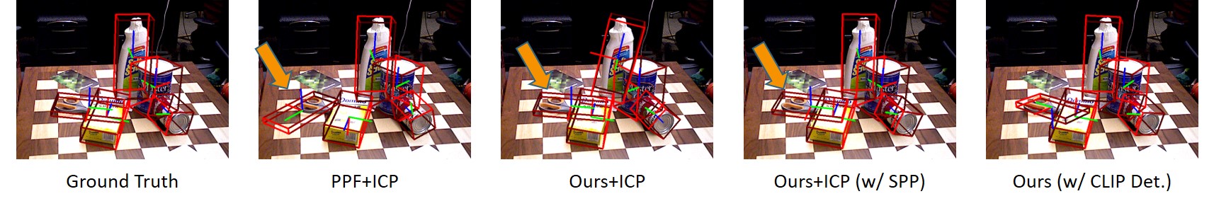
Figure 11: Qualitative comparison on YCB-Video dataset. Though not trained on cluttered objects, our method still gives decent results.

	PPF [33]		PPF [33]+ICP		Ours		Ours+ICP		Ours+ICP+SPP		Ours w/ CLIP Det.
Objects	ADD(-S)	ADD-S	ADD(-S)	ADD-S	ADD(-S)	ADD-S	ADD(-S)	ADD-S	ADD(-S)	ADD-S	ADD(-S)	ADD-S
master_chef_can	36.7	93.4	38.6	94.5	27.2	85.3	30.6	87.7	58.4	92.5	48.2	75.1
cracker_box	39.6	83.7	41.2	86.0	38.4	81.3	44.8	85.8	74.7	92.1	33.6	51.4
sugar_box	60.2	93.5	61.0	94.3	66.3	94.8	69.6	96.0	94.4	98.0	74.0	85.1
tomato_soup_can	56.8	94.0	56.9	94.6	60.4	93.6	62.0	94.1	90.2	94.7	74.8	77.5
mustard_bottle	60.3	91.1	64.9	92.4	57.5	88.2	64.5	91.5	60.8	90.2	66.0	95.5
tuna_fish_can	62.2	95.6	63.6	97.2	62.8	93.8	64.5	95.0	72.4	97.0	11.9	18.5
pudding_box	43.8	91.2	44.8	92.7	46.9	84.7	53.1	89.4	91.4	96.5	0.0	0.0
gelatin_box	70.4	96.6	78.2	97.5	81.7	97.0	93.7	98.1	96.3	98.6	35.9	36.0
potted_meat_can	56.2	79.4	58.3	80.4	54.8	78.3	55.2	78.9	64.7	79.3	29.9	36.0
banana	42.3	81.7	43.3	84.5	48.7	82.2	47.6	80.5	59.7	92.8	57.8	91.0
pitcher_base	11.1	26.7	13.0	27.6	10.4	27.8	12.1	28.1	10.7	25.0	66.7	91.9
bleach_cleanser	45.7	74.5	54.9	76.3	56.3	75.4	58.8	76.9	56.5	78.7	54.7	86.1
bowl	67.7	67.7	67.9	67.9	62.4	62.4	65.5	65.5	71.0	71.0	79.3	79.3
mug	39.7	91.6	40.7	92.0	41.8	91.6	42.9	91.9	48.5	92.8	59.4	81.5
power_drill	50.9	81.5	59.5	84.3	63.8	86.7	68.6	89.6	71.7	91.9	42.6	51.8
wood_block	71.4	71.4	72.0	72.0	69.1	69.1	69.5	69.5	61.7	61.7	88.1	88.1
scissors	20.4	67.7	26.9	75.1	53.0	85.3	46.1	86.4	54.8	87.8	32.8	66.2
large_marker	65.1	89.1	74.7	95.6	76.3	95.6	77.5	96.1	88.1	96.7	58.4	63.3
large_clamp	79.8	79.8	83.6	83.6	84.9	84.9	86.5	86.5	88.7	88.7	9.3	9.3
ex_large_clamp	37.1	37.1	39.2	39.2	40.4	40.4	42.3	42.3	44.6	44.6	1.1	1.1
foam_brick	89.5	89.5	90.1	90.1	88.9	88.9	90.3	90.3	90.6	90.6	46.0	46.0
ALL	52.0	81.6	55.2	83.4	55.4	81.8	58.0	83.4	70.0	85.5	46.8	59.3

TABLE V: AUC comparison between PPF and CPPF++(Ours) on YCB-Video dataset.

6.4 Comparison with Traditional PPF

Though our method is mainly designed for category-level pose estimation, interestingly, we find our method is superior than traditional PPF [8] in terms of instance-level pose estimation.

6.4.1 Datasets.

We use YCB-Video [38] dataset to evaluate our method on instance-level pose estimation, where the exact 3D model of the target object is known at training time. YCB-Video dataset consists of 21 objects and 92 RGB-D video sequences with pose annotations. We follow previous work [38] to evaluate on the 2,949 keyframes in 12 videos. Objects are placed arbitrarily on the table in the test frames.

6.4.2 Metrics.

We follow PoseCNN [38] to use the standard ADD(-S) and ADD-S metrics and report their area-under-the-curves (AUCs). The ADD metric is first introduced in  [13] to calculate average per-point distance between two point clouds, transformed by the predicted pose and the ground-truth, respectively. For symmetric objects like bowls, ADD-S metric is introduced to count for the point correspondence ambiguity. The notation ADD(-S) corresponds to computing ADD for non-symmetric objects and ADD-S for symmetric objects.

6.4.3 Baselines.

In the context of this paper, our primary objective is to enhance performance within a stringent sim-to-real framework. Consequently, we compare our methodology with PPF [33], which, akin to our approach, solely requires synthetic CAD models during the training phase. For a fair comparison, we use the readily available instance masks from PoseCNN [38] as the detection prior. For both methods, results after applying ICP are also given.

We acknowledge the emergence of recent sim-to-real techniques [10, 31, 35] that employ Blender for the rendering of hyper-realistic training images. Nonetheless, as highlighted in the introduction, these strategies introduce supplementary intricacies in the generation of backgrounds and disturbances. The extended duration required for data preparation and training renders them less feasible for real-world applications.

6.4.4 Results.

Table V presents the comprehensive results for each object within the YCB-Video dataset. Our approach surpasses PPF across nearly all metrics, both with and without the ICP cases. Notably, our method does not require exposure to object occlusion or background during training and can be seamlessly transitioned to real-world scenarios. Visual examples are showcased in Figure 11.

Furthermore, to differentiate poses for objects with ambiguous geometries, such as boxes, we incorporate a SuperPoint [7] based encoding technique to account for texture. This enhancement bolsters our method’s capability, particularly when dealing with textured symmetric objects. Specifically, in conjunction with the tuple features elaborated in Equation 3.5, we concatenate the interpolated per-point SuperPoint feature for each tuple. This integration of color and texture information aids our model in more accurately handling symmetric geometric objects.

Moreover, we also present results utilizing the CLIP fine-tuned instance segmentation detector with Grounded SAM, as detailed in Section 3.6. While it exhibits proficiency in certain categories, its zero-shot detection performance for many objects remains suboptimal, leading to a decline in both ADD(-S) and ADD-S metrics.

6.4.5 Detailed Analysis and Failure Cases.

Due to the results in Table V, we find that although our method is effective in almost all the instances, there is a significant performance drop for the instance $pitcher\_base$. This is caused by the substantial failure of instance segmentation. The detector provided by PoseCNN [38] fails to detect a majority of $pitcher\_base$ instances. When we use our fine-tuned CLIP detection, the performance returns to normal. A qualitative comparison of $pitcher\_base$ detections between the PoseCNN detector and the CLIP detector is given in Figure 12.

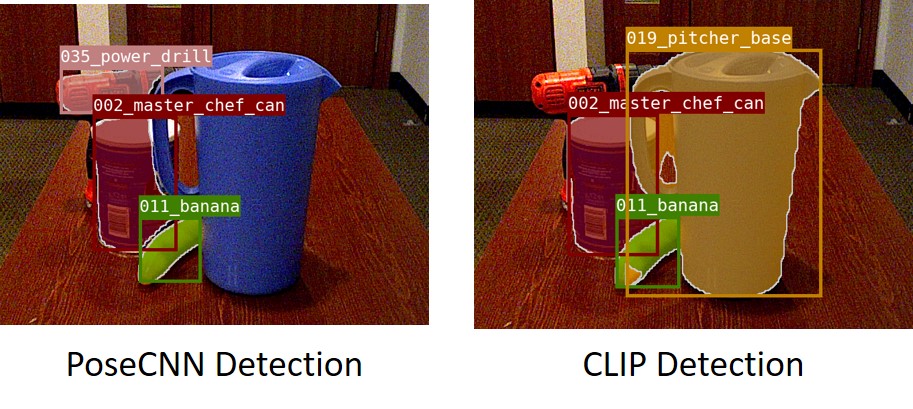
Figure 12: A qualitative comparison of the instance segmentation results between the pretrained model provided by PoseCNN and the CLIP finetuned model. The PoseCNN pretrained model perform badly on the object $pitcher\_base$ while the CLIP model works well on this object. On the other hand, the CLIP finetuned model fails to detect the challenging instance $power\_drill$ due to the large occlusion.

7 Conclusion and Limitations

This paper presents the innovative CPPF++ method tailored for sim-to-real pose estimation. Rooted in the foundational point-pair voting scheme of CPPF, our approach reinterprets it using a probabilistic perspective. To counteract voting collision, we innovatively model voting uncertainty by gauging the probabilistic distribution of each point pair in the canonical space, complemented by an iterative noise filtering technique to eliminate votes linked to backgrounds or clutters. Our method also introduces the concept of $N$-point tuples, enhancing the context of each voting unit by amalgamating pair-wise features from multiple points. Alongside this, we unveil the DiversePose 300 dataset, curated to provide a comprehensive assessment of top-tier methods in diverse real-world conditions. Our empirical findings validate the effectiveness of CPPF++, highlighting a marked decrease in the gap between simulated and real-world performance in both instance and category-level contexts.

Our model does not predict object size very well mainly because of the simple averaging voting scheme for the size. One potential future improvement is to learning a size prior and optimize the size in post-processing. Besides, our method heavily depends on the depth input to predict the pose. It is more general and helpful to use RGB colors only, by exploring a novel voting strategy in the image plane.

References

- [1] Adel Ahmadyan, Liangkai Zhang, Artsiom Ablavatski, Jianing Wei, and Matthias Grundmann. Objectron: A large scale dataset of object-centric videos in the wild with pose annotations. In Proceedings of the IEEE/CVF Conference on Computer Vision and Pattern Recognition, pages 7822–7831, 2021.
- [2] Angel X. Chang, Thomas Funkhouser, Leonidas Guibas, Pat Hanrahan, Qixing Huang, Zimo Li, Silvio Savarese, Manolis Savva, Shuran Song, Hao Su, Jianxiong Xiao, Li Yi, and Fisher Yu. ShapeNet: An Information-Rich 3D Model Repository. Technical Report arXiv:1512.03012 [cs.GR], Stanford University — Princeton University — Toyota Technological Institute at Chicago, 2015.
- [3] Dengsheng Chen, Jun Li, Zheng Wang, and Kai Xu. Learning canonical shape space for category-level 6d object pose and size estimation. In Proceedings of the IEEE/CVF conference on computer vision and pattern recognition, pages 11973–11982, 2020.
- [4] Wei Chen, Xi Jia, Hyung Jin Chang, Jinming Duan, Linlin Shen, and Ales Leonardis. Fs-net: Fast shape-based network for category-level 6d object pose estimation with decoupled rotation mechanism. In Proceedings of the IEEE/CVF Conference on Computer Vision and Pattern Recognition, pages 1581–1590, 2021.
- [5] Xu Chen, Zijian Dong, Jie Song, Andreas Geiger, and Otmar Hilliges. Category level object pose estimation via neural analysis-by-synthesis. In European Conference on Computer Vision, pages 139–156. Springer, 2020.
- [6] Xinke Deng, Yu Xiang, Arsalan Mousavian, Clemens Eppner, Timothy Bretl, and Dieter Fox. Self-supervised 6d object pose estimation for robot manipulation. In 2020 IEEE International Conference on Robotics and Automation (ICRA), pages 3665–3671. IEEE, 2020.
- [7] Daniel DeTone, Tomasz Malisiewicz, and Andrew Rabinovich. Superpoint: Self-supervised interest point detection and description. In Proceedings of the IEEE conference on computer vision and pattern recognition workshops, pages 224–236, 2018.
- [8] Bertram Drost, Markus Ulrich, Nassir Navab, and Slobodan Ilic. Model globally, match locally: Efficient and robust 3d object recognition. In 2010 IEEE computer society conference on computer vision and pattern recognition, pages 998–1005. Ieee, 2010.
- [9] Ge Gao, Mikko Lauri, Yulong Wang, Xiaolin Hu, Jianwei Zhang, and Simone Frintrop. 6d object pose regression via supervised learning on point clouds. In 2020 IEEE International Conference on Robotics and Automation (ICRA), pages 3643–3649. IEEE, 2020.
- [10] Rasmus Laurvig Haugaard and Anders Glent Buch. Surfemb: Dense and continuous correspondence distributions for object pose estimation with learnt surface embeddings. In Proceedings of the IEEE/CVF Conference on Computer Vision and Pattern Recognition, pages 6749–6758, 2022.
- [11] Kaiming He, Georgia Gkioxari, Piotr Dollár, and Ross Girshick. Mask r-cnn. In Proceedings of the IEEE international conference on computer vision, pages 2961–2969, 2017.
- [12] Kaiming He, Xiangyu Zhang, Shaoqing Ren, and Jian Sun. Deep residual learning for image recognition. In Proceedings of the IEEE conference on computer vision and pattern recognition, pages 770–778, 2016.
- [13] Stefan Hinterstoisser, Vincent Lepetit, Slobodan Ilic, Stefan Holzer, Gary Bradski, Kurt Konolige, and Nassir Navab. Model based training, detection and pose estimation of texture-less 3d objects in heavily cluttered scenes. In Asian conference on computer vision, pages 548–562. Springer, 2012.
- [14] Tomáš Hodaň, Martin Sundermeyer, Bertram Drost, Yann Labbé, Eric Brachmann, Frank Michel, Carsten Rother, and Jiří Matas. Bop challenge 2020 on 6d object localization. In European Conference on Computer Vision, pages 577–594. Springer, 2020.
- [15] Muhammad Zubair Irshad, Thomas Kollar, Michael Laskey, Kevin Stone, and Zsolt Kira. Centersnap: Single-shot multi-object 3d shape reconstruction and categorical 6d pose and size estimation. arXiv preprint arXiv:2203.01929, 2022.
- [16] Muhammad Zubair Irshad, Sergey Zakharov, Rares Ambrus, Thomas Kollar, Zsolt Kira, and Adrien Gaidon. Shapo: Implicit representations for multi-object shape, appearance, and pose optimization. arXiv preprint arXiv:2207.13691, 2022.
- [17] Alexander Kirillov, Eric Mintun, Nikhila Ravi, Hanzi Mao, Chloe Rolland, Laura Gustafson, Tete Xiao, Spencer Whitehead, Alexander C Berg, Wan-Yen Lo, et al. Segment anything. arXiv preprint arXiv:2304.02643, 2023.
- [18] Yann Labbé, Justin Carpentier, Mathieu Aubry, and Josef Sivic. Cosypose: Consistent multi-view multi-object 6d pose estimation. In European Conference on Computer Vision, pages 574–591. Springer, 2020.
- [19] Feng Li, Hao Zhang, Huaizhe Xu, Shilong Liu, Lei Zhang, Lionel M Ni, and Heung-Yeung Shum. Mask dino: Towards a unified transformer-based framework for object detection and segmentation. In Proceedings of the IEEE/CVF Conference on Computer Vision and Pattern Recognition, pages 3041–3050, 2023.
- [20] Yi Li, Gu Wang, Xiangyang Ji, Yu Xiang, and Dieter Fox. Deepim: Deep iterative matching for 6d pose estimation. In Proceedings of the European Conference on Computer Vision (ECCV), pages 683–698, 2018.
- [21] Haitao Lin, Zichang Liu, Chilam Cheang, Yanwei Fu, Guodong Guo, and Xiangyang Xue. Sar-net: Shape alignment and recovery network for category-level 6d object pose and size estimation. In Proceedings of the IEEE/CVF Conference on Computer Vision and Pattern Recognition, pages 6707–6717, 2022.
- [22] Jiehong Lin, Zewei Wei, Zhihao Li, Songcen Xu, Kui Jia, and Yuanqing Li. Dualposenet: Category-level 6d object pose and size estimation using dual pose network with refined learning of pose consistency. In Proceedings of the IEEE/CVF International Conference on Computer Vision (ICCV), pages 3560–3569, October 2021.
- [23] Shilong Liu, Zhaoyang Zeng, Tianhe Ren, Feng Li, Hao Zhang, Jie Yang, Chunyuan Li, Jianwei Yang, Hang Su, Jun Zhu, et al. Grounding dino: Marrying dino with grounded pre-training for open-set object detection. arXiv preprint arXiv:2303.05499, 2023.
- [24] Matthew Matl. Pyrender. https://github.com/mmatl/pyrender, 2018.
- [25] Van Nguyen Nguyen, Yinlin Hu, Yang Xiao, Mathieu Salzmann, and Vincent Lepetit. Templates for 3d object pose estimation revisited: Generalization to new objects and robustness to occlusions. In Proceedings of the IEEE/CVF Conference on Computer Vision and Pattern Recognition, pages 6771–6780, 2022.
- [26] Alec Radford, Jong Wook Kim, Chris Hallacy, Aditya Ramesh, Gabriel Goh, Sandhini Agarwal, Girish Sastry, Amanda Askell, Pamela Mishkin, Jack Clark, et al. Learning transferable visual models from natural language supervision. In International conference on machine learning, pages 8748–8763. PMLR, 2021.
- [27] Radu Bogdan Rusu and Steve Cousins. 3d is here: Point cloud library (pcl). In 2011 IEEE international conference on robotics and automation, pages 1–4. IEEE, 2011.
- [28] Samuele Salti, Federico Tombari, and Luigi Di Stefano. Shot: Unique signatures of histograms for surface and texture description. Computer Vision and Image Understanding, 125:251–264, 2014.
- [29] Stefan Stevšić, Sammy Christen, and Otmar Hilliges. Learning to assemble: Estimating 6d poses for robotic object-object manipulation. IEEE Robotics and Automation Letters, 5(2):1159–1166, 2020.
- [30] Yongzhi Su, Jason Rambach, Nareg Minaskan, Paul Lesur, Alain Pagani, and Didier Stricker. Deep multi-state object pose estimation for augmented reality assembly. In 2019 IEEE International Symposium on Mixed and Augmented Reality Adjunct (ISMAR-Adjunct), pages 222–227. IEEE, 2019.
- [31] Martin Sundermeyer, Tomáš Hodaň, Yann Labbe, Gu Wang, Eric Brachmann, Bertram Drost, Carsten Rother, and Jiří Matas. Bop challenge 2022 on detection, segmentation and pose estimation of specific rigid objects. In Proceedings of the IEEE/CVF Conference on Computer Vision and Pattern Recognition, pages 2784–2793, 2023.
- [32] Meng Tian, Marcelo H Ang, and Gim Hee Lee. Shape prior deformation for categorical 6d object pose and size estimation. In European Conference on Computer Vision, pages 530–546. Springer, 2020.
- [33] Joel Vidal, Chyi-Yeu Lin, and Robert Martí. 6d pose estimation using an improved method based on point pair features. In 2018 4th international conference on control, automation and robotics (iccar), pages 405–409. IEEE, 2018.
- [34] Chen Wang, Danfei Xu, Yuke Zhu, Roberto Martín-Martín, Cewu Lu, Li Fei-Fei, and Silvio Savarese. Densefusion: 6d object pose estimation by iterative dense fusion. In Proceedings of the IEEE/CVF conference on computer vision and pattern recognition, pages 3343–3352, 2019.
- [35] Gu Wang, Fabian Manhardt, Federico Tombari, and Xiangyang Ji. Gdr-net: Geometry-guided direct regression network for monocular 6d object pose estimation. In Proceedings of the IEEE/CVF Conference on Computer Vision and Pattern Recognition, pages 16611–16621, 2021.
- [36] He Wang, Srinath Sridhar, Jingwei Huang, Julien Valentin, Shuran Song, and Leonidas J Guibas. Normalized object coordinate space for category-level 6d object pose and size estimation. In Proceedings of the IEEE/CVF Conference on Computer Vision and Pattern Recognition, pages 2642–2651, 2019.
- [37] Yangzheng Wu, Mohsen Zand, Ali Etemad, and Michael Greenspan. Vote from the center: 6 dof pose estimation in rgb-d images by radial keypoint voting. In European Conference on Computer Vision (ECCV). Springer, 2022.
- [38] Yu Xiang, Tanner Schmidt, Venkatraman Narayanan, and Dieter Fox. Posecnn: A convolutional neural network for 6d object pose estimation in cluttered scenes. 2018.
- [39] Yang You, Ruoxi Shi, Weiming Wang, and Cewu Lu. Cppf: Towards robust category-level 9d pose estimation in the wild. In Proceedings of the IEEE/CVF Conference on Computer Vision and Pattern Recognition, pages 6866–6875, 2022.
- [40] Xu Zhao, Wenchao Ding, Yongqi An, Yinglong Du, Tao Yu, Min Li, Ming Tang, and Jinqiao Wang. Fast segment anything. arXiv preprint arXiv:2306.12156, 2023.
- [41] Linfang Zheng, Chen Wang, Yinghan Sun, Esha Dasgupta, Hua Chen, Aleš Leonardis, Wei Zhang, and Hyung Jin Chang. Hs-pose: Hybrid scope feature extraction for category-level object pose estimation. In Proceedings of the IEEE/CVF Conference on Computer Vision and Pattern Recognition, pages 17163–17173, 2023.
- [42] Chengliang Zhong, Chao Yang, Fuchun Sun, Jinshan Qi, Xiaodong Mu, Huaping Liu, and Wenbing Huang. Sim2real object-centric keypoint detection and description. In Proceedings of the AAAI Conference on Artificial Intelligence, volume 36, pages 5440–5449, 2022.