A Riemannian exponential augmented Lagrangian method for computing the projection robust Wasserstein distance

Abstract

Projecting the distance measures onto a low-dimensional space is an efficient way of mitigating the curse of dimensionality in the classical Wasserstein distance using optimal transport. The obtained maximized distance is referred to as projection robust Wasserstein (PRW) distance. In this paper, we equivalently reformulate the computation of the PRW distance as an optimization problem over the Cartesian product of the Stiefel manifold and the Euclidean space with additional nonlinear inequality constraints. We propose a Riemannian exponential augmented Lagrangian method (ReALM) with a global convergence guarantee to solve this problem. Compared with the existing approaches, ReALM can potentially avoid too small penalty parameters. Moreover, we propose a framework of inexact Riemannian gradient descent methods to solve the subproblems in ReALM efficiently. In particular, by using the special structure of the subproblem, we give a practical algorithm named as the inexact Riemannian Barzilai-Borwein method with Sinkhorn iteration (iRBBS). The remarkable features of iRBBS lie in that it performs a flexible number of Sinkhorn iterations to compute an inexact gradient with respect to the projection matrix of the problem and adopts the Barzilai-Borwein stepsize based on the inexact gradient information to improve the performance. We show that iRBBS can return an $\epsilon$-stationary point of the original PRW distance problem within $\mathcal{O}(\epsilon^{-3})$ iterations. Extensive numerical results on synthetic and real datasets demonstrate that our proposed ReALM as well as iRBBS outperform the state-of-the-art solvers for computing the PRW distance.

65K10, 90C26, 90C47

1 Introduction

The optimal transport (OT) problem has wide applications in machine learning, data sciences, and image sciences; see [36] and the references therein for more details. However, its direct application in machine learning may encounter the curse of dimensionality issue since the sample complexity of approximating the Wasserstein distance can grow exponentially in dimension [18, 42]. To resolve this issue, by making an important extension to the sliced Wasserstein distance, Paty and Cuture [35] and Niles-Wee and Rigollet [34] proposed to project the distributions to a $k$-dimensional subspace that maximizes the Wasserstein distance, which can reduce the sample complexity and overcome the issue of the curse of dimensionality [34, 31].

In this paper, we focus on the discrete probability measures case. For $\{x_{1},\ldots,x_{n}\}$
$\subset\mathbb{R}^{d}$ and $\{y_{1},\ldots,y_{n}\}\subset\mathbb{R}^{d}$, define ${\color[rgb]{0,0,0}{M_{ij}}}=(x_{i}-y_{j})(x_{i}-y_{j})^{\mathsf{T}}$ for each $(i,j)$. Let $\mathbf{1}\in\mathbb{R}^{n}$ be the all-one vector and $\delta_{x}$ be the Dirac delta function at $x$. Consider two discrete probability measures $\mu_{n}=\sum_{i=1}^{n}r_{i}\delta_{x_{i}}$ and $\nu_{n}=\sum_{i=1}^{n}c_{i}\delta_{y_{i}}$, where $r,c\in\Delta^{n}:=\{z\in\mathbb{R}^{n}\mid\mathbf{1}^{\mathsf{T}}z=1,z>0\}$. For the integer $1\leq k\leq d$, the $k$-dimensional projection robust Wasserstein (PRW) distance between $\mu_{n}$ and $\nu_{n}$ is defined as [35]

(1) $$\mathcal{P}_{k}^{2}(\mu_{n},\nu_{n})=\max_{U\in\mathcal{S}}\min_{\pi\in\Pi(r,c)}f(\pi,U),$$

where $f(\pi,U)=\left\langle\pi,C(U)\right\rangle$ with $C(U)\in\mathbb{R}^{n\times n}$ and $[C(U)]_{ij}=\left\langle M_{ij},UU^{\mathsf{T}}\right\rangle$. Throughout this paper, $\mathcal{S}=\{U\in\mathbb{R}^{d\times k}\mid U^{\mathsf{T}}U=I_{k}\}$ is known as the Stiefel manifold with $I_{k}$ being the $k\times k$ identity matrix and $\Pi(r,c)=\{\pi\in\mathbb{R}^{n\times n}\mid\pi\mathbf{1}=r,\pi^{\mathsf{T}}\mathbf{1}=c,\pi\geq 0\}$. Problem (1) is a nonconcave-convex max-min problem over the Stiefel manifold, which makes it very challenging to solve.

1.1 Related works

To compute the PRW distance, [35] considered a convex relaxation (but without the theoretical guarantee on the duality gap), wherein an OT or entropy-regularized OT subproblem with dimension $n$ needs to be solved exactly in each step. Very recently, Lin et al. [29] viewed problem (1) as a single-level optimization problem over the Stiefel manifold:

(2) $$\max_{U\in\mathcal{S}}\,p(U),$$

where $p(U)=\min_{\pi\in\Pi(r,c)}f(\pi,U)$. Observe that $p(U)$ is a weakly convex [29, Lemma 2.2] but nonsmooth function. Then it is possible to use the Riemannian subgradient method developed in [28] to solve (2). However, this may still be difficult since computing a subgradient of $p(\cdot)$ at $U$ needs to solve an OT problem exactly. Instead of solving (2) directly, Lin et al. [29] considered solving the following regularization problem with a small regularization parameter $\eta$:

(3) $$\max_{U\in\mathcal{S}}\,p_{\eta}(U),$$

where $p_{\eta}(U)=\min_{\pi\in\Pi(r,c)}f(\pi,U)-\eta H(\pi)$, in which $H(\pi)=-\sum_{ij}\pi_{ij}\log\pi_{ij}$ is the entropy function. To solve problem (3), Lin et al. [29] proposed a Riemannian (adaptive) gradient ascent with Sinkhorn (R(A)GAS) algorithm, which can be understood as a Riemannian gradient ascent method with an inexact gradient at a fixed inexactness level. They showed that R(A)GAS can return an $\epsilon$-stationary point (see Definition 2.7 in [29]) of PRW (1) in $\mathcal{O}(\epsilon^{-4})$ iterations if $\eta=\mathcal{O}(\epsilon)$ in (3). However, in each iteration, R(A)GAS needs to calculate $\nabla p_{\eta}(U)$ via solving a regularized OT problem in relatively high precision, which results in a high computational cost.

To further reduce the complexity of R(A)GAS, rather than solving (3) directly, Huang et al. [22] focused on an equivalent “min” formulation of (3)

(4) $$\min_{U\in\mathcal{S},\alpha,\beta\in\mathbb{R}^{n}}h_{\eta}(\alpha,\beta,U)$$

via replacing $p_{\eta}(U)$ by its dual, that is $p_{\eta}(U)=\max_{\alpha,\beta\in\mathbb{R}^{n}}-h_{\eta}(\alpha,\beta,U),$ where

$$h_{\eta}(\alpha,\beta,U)=r^{\mathsf{T}}\alpha+c^{\mathsf{T}}\beta+\eta\log\sum\nolimits_{ij}\exp\left(-\frac{\alpha_{i}+\beta_{j}+\langle M_{ij},UU^{\mathsf{T}}\rangle}{\eta}\right).$$

Note that the last term in $h_{\eta}(\alpha,\beta,U)$ is also known as the log-exponential aggregation function [27]. Huang et al. [22] proposed two efficient algorithms, named Riemannian (adaptive) block coordinate descent (R(A)BCD) algorithms to solve (4). In their algorithms, $\alpha$ and $\beta$ are updated by one Sinkhorn iteration, while $U$ is updated by a Riemannian gradient descent step with a fixed stepsize. By choosing $\eta=\mathcal{O}(\epsilon)$ in (4), they showed that the whole iteration complexity of R(A)BCD to attain an $\epsilon$-stationary point (see [22, Definition 4.1] wherein $\epsilon_{1}=\epsilon_{2}=\epsilon$) of PRW (1) is reduced to $\mathcal{O}(\epsilon^{-3})$, which significantly improves the complexity of R(A)GAS [22].

However, as pointed out in [22, Remark 6.1], there are two main issues of R(A)BCD
and R(A)GAS. First, the algorithms are sensitive to the choice of parameter $\eta$. More specifically, to compute a solution with relatively high quality, $\eta$ has to be chosen to be small, which may cause numerical instability. Second, the performance of the algorithms is sensitive to the stepsizes in updating $U$. Hence, to achieve a better performance, one has to spend some efforts to tune the stepsizes carefully. Resolving the two main issues of R(A)BCD demands some novel approach from both theoretical and computational points of view, and this is the focus of our paper.

To handle the first issue mentioned above, we first observe that the approach proposed by Huang et al. [22] can be understood as a Riemannian exponential penalty method applied to an equivalent formulation (8) of (2); see Remark 2.8 later. On the other hand, the exponential augmented Lagrangian methods (ALM), which are usually more stable than the exponential penalty type of methods, have been well-studied [6, 40] and widely used to solve various problems, such as optimal transport [45], semidefinite programming [14], equilibrium problems [39], etc. Hence, our idea for resolving the first issue is to extend the exponential ALM from the Euclidean case to the Riemannian case. It should be remarked that for the fixed subspace $U$ case, such an idea has been adopted in computing the standard OT problem, wherein a proximal point-based entropy subproblem with a positive constant $\eta$ needs to be solved inexactly in each iteration; see [44, 45] for more details.

Problem (4) can also be viewed as a single-level optimization over the Stiefel manifold by letting $h_{\eta}(U)=\min_{\alpha,\beta\in\mathbb{R}^{n}}h_{\eta}(\alpha,\beta,U)$. Our idea for resolving the second issue lies in using an inexact Riemannian gradient descent method to solve $\min_{U\in\mathcal{S}}h_{\eta}(U)$, wherein the Riemannian gradient $\operatorname{grad}h_{\eta}(U)$ is computed inexactly at an adaptive inexactness level. Although the inexact gradient descent method has been well explored in the Euclidean case [10, 13, 5], to our best knowledge, there are no results on how to choose the stepsize adaptively for general nonlinear objective functions. One exception is [21], where for the strongly convex quadratic objective function, Hu and Dai proposed an inexact Barzilai-Borwein (BB) method and established the R-linear convergence of the inexact BB method if the inexactitude of the approximate gradient is well controlled. However, the method in [21] can not be directly extended to solve problem (4) due to the lack of the appropriate line search condition. Motivated by Hu and Dai’s method and successful extensions of the BB method [4] to the Riemannian case [43, 25, 19, 24], our solution to the second issue is to develop an inexact Riemannian gradient descent method with the BB stepsize and an appropriate nonmonotone line search condition.

1.2 Our contributions

In this paper, by reformulating (1) as an optimization problem defined over the Cartesian product of the Stiefel manifold and the Euclidean space with additional inequality constraints (see (8) further ahead), we design a Riemannian exponential ALM (ReALM) with customized methods for solving the subproblems to efficiently and faithfully compute the PRW distance. Our main contributions are summarized as follows.

• We propose a ReALM method for computing the PRW distance, in which a series of subproblems with dynamically decreasing penalty parameters and adaptively updated multiplier matrices is solved approximately. In theory, we establish the global convergence of ReALM in the sense that any limit point of the sequence generated by the algorithm is a stationary point of the original problem. Numerically, ReALM always outperforms the Riemannian exponential penalty approach, which solves a series of subproblems with dynamically decreasing penalty parameters or with a sufficiently small penalty parameter. In particular, our method can avoid too small penalty parameters in some cases compared with the Riemannian exponential penalty approach.

• To efficiently solve the subproblem (4) or (13), we propose a framework of inexact Riemannian gradient descent (iRGD) methods with convergence and complexity guarantees. Particularly, we give a practical algorithm, namely, the inexact Riemannian BB method with Sinkhorn iteration (iRBBS), wherein a flexible number of Sinkhorn iterations is performed to compute an inexact gradient with respect to the projection matrix. Compared with R(A)BCD, our proposed iRBBS can not only return a stronger $(\epsilon_{1},\epsilon_{2})$-stationary point of PRW (1), compared with the definitions in [29, 22], in $\mathcal{O}(\max\{\epsilon_{1}^{-2},\epsilon_{2}^{-2}\}\epsilon_{2}^{-1})$ iterations (see Corollary 4.12 and Remark 2.4), but also has a better numerical performance, which mainly benefits from the inexact BB stepsize. As a by-product, we also establish the complexity results of the original Sinkhorn iteration in a simple way.

1.3 Notations and preliminaries

For a scalar $a$, let $\lceil a\rceil$ be the smallest nonnegative integer larger than $a$. Denote $[n]=\{1,2,\ldots,n\}$. For a matrix $A$, denote $A_{\min}=\min_{ij}A_{ij}$. Denote by $\|A\|_{\mathsf{F}}$ the Frobenius norm of $A$. The $\ell_{\infty}$-norm of $A$ is $\|A\|_{\infty}=\max_{ij}|A|_{ij}$, while the $\ell_{1}$-norm is $\|A\|_{1}=\sum_{ij}|A_{ij}|$. The variation seminorm of $A$ is $\|A\|_{\mathrm{var}}=\max_{ij}A_{ij}-\min_{ij}A_{ij}$. The notation $\log A$ denotes a matrix of the same size as $A$, and $(\log A)_{ij}=\log A_{ij}$. For a vector $x\in\mathbb{R}^{n}$, $\operatorname{Diag}(x)$ is an $n\times n$ diagonal matrix with $x$ being its main diagonal. We use $\mathbb{R}_{+}^{n\times n}$ and $\mathbb{R}_{++}^{n\times n}$ to denote the nonnegative and positive orthants of $\mathbb{R}^{n\times n}$, respectively. The entropy function is given as $H(\pi)=-\sum_{ij}\pi_{ij}\log\pi_{ij}$ for $\pi\in\mathbb{R}^{n\times n}_{+}$ and $\|\pi\|_{1}=1$ with the convention that $H(\pi)=-\infty$ if one of the entries $\pi_{ij}=0$. For $p,q\in\Delta^{n}$, the Kullbbback-Leibler divergence between $p$ and $q$ is $\mathsf{KL}(p\|q)=\sum_{i}p_{i}\log(p_{i}/q_{i})$. Throughout this paper, we define the matrix $C\in\mathbb{R}^{n\times n}$ with $C_{ij}=\|x_{i}-y_{j}\|^{2}$ and define $V_{\pi}=\sum_{ij}\pi_{ij}M_{ij}$.

The Riemannian metric endowed on the Stiefel manifold $\mathcal{S}$ is taken as the usual metric on $\mathbb{R}^{d\times k}$. The tangent space at $U\in\mathcal{S}$ is $\mathrm{T}_{U}\mathcal{S}=\{\xi\in\mathbb{R}^{d\times k}\mid U^{\mathsf{T}}\xi+\xi^{\mathsf{T}}U=0\}$. Let $\mathrm{T}\mathcal{S}=\{(U,\xi)\mid U\in\mathcal{S}\mbox{ and }\xi\in\mathrm{T}_{U}\mathcal{S}\}$ be the tangent bundle of $\mathcal{S}$. A smooth map $\mathsf{Retr}:\mathrm{T}\mathcal{S}\to\mathcal{S}:(U,\xi)\mapsto\mathsf{Retr}_{U}(\xi)$ is called a retraction if each curve $\mathcal{R}(t)=\mathsf{Retr}_{U}(t\xi)$ satisfies $\mathcal{R}(0)=U$ and $\mathcal{R}^{\prime}(0)=\xi$; see [8, Definition 3.47] or [1, Definition 4.1.1]. The retraction on the Stiefel manifold has the following nice properties; see [32, 9] for instance.

Fact 1.

There exist positive constants $L_{1}$ and $L_{2}$ such that $\|\mathsf{Retr}_{U}(\xi)-U\|_{\mathsf{F}}\leq L_{1}\|\xi\|_{\mathsf{F}}$ and $\|\mathsf{Retr}_{U}(\xi)-(U+\xi)\|_{\mathsf{F}}\leq L_{2}\|\xi\|_{\mathsf{F}}^{2}$ hold for all $\xi\in\mathrm{T}_{U}\mathcal{S}$ and $U\in\mathcal{S}$.

The Riemannian gradient of a smooth function $f:\mathbb{R}^{d\times k}\to\mathbb{R}$ at $U$ is defined as $\operatorname{grad}f(U)$, which satisfies $\left\langle\operatorname{grad}f(U),\xi\right\rangle=\left\langle\nabla f(U),\xi\right\rangle$ for all $\xi\in\mathrm{T}_{U}\mathcal{S}$. If $U^{\mathsf{T}}\nabla f(U)$ is symmetric, we have $\operatorname{grad}f(U)=\mathsf{Proj}_{\mathrm{T}_{U}\mathcal{S}}(\nabla f(U))=(I_{d}-UU^{\mathsf{T}})\nabla f(U).$

1.4 Organization

The rest of this paper is organized as follows. The proposed ReALM method is introduced in Section 2. A framework of inexact RGD methods and a practical iRBBS for solving the subproblem in ReALM are proposed in Section 3 and Section 4, respectively. Numerical results are presented in Section 5. Finally, we draw some concluding remarks in Section 6.

2 A ReALM for computing the PRW distance (1)

In this section, we first give a reformulation of PRW distance problem (1) in section 2.1 and then propose a Riemannian exponential ALM, summarized as Algorithm 1, for solving the reformulation problem in section 2.2. The global convergence of Algorithm 1 is discussed in section 2.3.

2.1 Reformulation of PRW distance problem (1)

Motivated by the dual approach in [22], we first rewrite (1) as an optimization problem over the Cartesian product of the Stiefel manifold and the Euclidean space with additional nonlinear inequality constraints.

Given a fixed $U\in\mathcal{S}$, consider the OT problem

(5) $$\min_{\pi\in\mathbb{R}^{n\times n}}\left\langle\pi,C(U)\right\rangle\quad\mathrm{s.t.}\quad\pi\mathbf{1}=r,~{}~{}\pi^{\mathsf{T}}\mathbf{1}=c,~{}~{}\pi\geq 0.$$

Let $\hat{\mathcal{L}}(\pi,\alpha,\beta)=\left\langle\pi,C(U)\right\rangle+\langle\alpha,\pi\mathbf{1}-r\rangle+\langle\beta,\pi^{\mathsf{T}}\mathbf{1}-c\rangle$ be the Lagrangian function with $\alpha\in\mathbb{R}^{n}$ and $\beta\in\mathbb{R}^{n}$ being the Lagrange multipliers corresponding to the constraints $\pi\mathbf{1}=r$ and $\pi^{\mathsf{T}}\mathbf{1}=c$, respectively. As done in [22, 30] for deriving the dual of the entropy-regularized OT problem, we add a redundant constraint $\|\pi\|_{1}=1$ and derive the dual problem of (5) as $\max_{\alpha\in\mathbb{R}^{n},\beta\in\mathbb{R}^{n}}\min_{\pi\geq 0,\|\pi\|_{1}=1}\hat{\mathcal{L}}(\pi,\alpha,\beta),$ that is,

$$\max\limits_{\alpha\in\mathbb{R}^{n},\beta\in\mathbb{R}^{n}}-h(\mathbf{x}),$$

where $\mathbf{x}=(\alpha,\beta,U)$ and

(6) $$h(\mathbf{x})=r^{\mathsf{T}}\alpha+c^{\mathsf{T}}\beta-\varphi(\mathbf{x})_{\min}\quad\mbox{with}\quad\varphi_{ij}(\mathbf{x})=\alpha_{i}+\beta_{j}+\langle{\color[rgb]{0,0,0}{M_{ij}}},UU^{\mathsf{T}}\rangle.$$

Therefore, the PRW distance between $\mu_{n}$ and $\nu_{n}$ defined in (1) is equal to

(7) $$\mathcal{P}_{k}^{2}(\mu_{n},\nu_{n})=-\min\limits_{\mathbf{x}\in\mathcal{M}}h(\mathbf{x}),$$

where $\mathcal{M}=\mathbb{R}^{n}\times\mathbb{R}^{n}\times\mathcal{S}.$ The corresponding minimization problem in (7) can be reformulated as the minimization problem as

(8) $$\min\limits_{\mathbf{x}\in\mathcal{M},y\in\mathbb{R}}\ r^{\mathsf{T}}\alpha+c^{\mathsf{T}}\beta+y\quad\mathrm{s.t.}\quad\varphi_{ij}(\mathbf{x})+y\geq 0,\quad\forall~{}i,j\in[n].$$

In this paper, we shall focus on the formulation (8), whose first-order necessary conditions are established as follows.

Lemma 2.1 (First-order necessary conditions).

Given $\bar{\mathbf{x}}\in\mathcal{M}$ and $\bar{y}\in\mathbb{R}$, suppose that $(\bar{\mathbf{x}},\bar{y})$ is a local minimizer of problem (8), then $(\bar{\mathbf{x}},-\varphi(\bar{\mathbf{x}})_{\min})$ is a stationary point of problem (8), namely, there exists $\bar{\pi}\in\Pi(r,c)$ such that

(9) $$\mathsf{Proj}_{\mathrm{T}_{\bar{U}}\mathcal{S}}\left(-2V_{\bar{\pi}}\bar{U}\right)=0,\quad\left\langle\bar{\pi},Z(\bar{\mathbf{x}})\right\rangle=0,$$

where $Z(\bar{\mathbf{x}})\in\mathbb{R}^{n\times n}$ with

(10) $$[Z(\bar{\mathbf{x}})]_{ij}=\varphi_{ij}(\bar{\mathbf{x}})-\varphi(\bar{\mathbf{x}})_{\min}.$$

Proof 2.2.

Since $(\bar{\mathbf{x}},\bar{y})$ is a local minimizer of problem (8), there must hold $\bar{y}=-\varphi(\bar{\mathbf{x}})_{\min}=\max_{ij}\{-\varphi_{ij}(\bar{\mathbf{x}})\}$. Moreover, such $\bar{\mathbf{x}}$ is also a local minimizer of problem $\min_{\mathbf{x}\in\mathcal{M}}h(\mathbf{x})$, where $h(\mathbf{x})$ is given in (6). For fixed $\alpha$ and $\beta$, it is easy to see that $-\varphi_{ij}(\mathbf{x})+\|C\|_{\infty}\|U\|_{\mathsf{F}}^{2}$ is convex with respect to $U$. We thus know that the function $-\varphi(\bar{\mathbf{x}})_{\min}+\|C\|_{\infty}\|U\|_{\mathsf{F}}^{2}=\max_{ij}\left\{-\varphi_{ij}(\mathbf{x})+\|C\|_{\infty}\|U\|_{\mathsf{F}}^{2}\right\}$ is convex with respect to $U$, which means that the function $-\varphi(\bar{\mathbf{x}})_{\min}$ and thus $h(\mathbf{x})$ is $\|C\|_{\infty}$-weakly convex with respect to $U$ [41, Proposition 4.3]. Let $\mathcal{A}(\bar{\mathbf{x}})=\{(i,j)\in[n]\times[n]\mid\varphi_{ij}(\bar{\mathbf{x}})=\varphi(\bar{\mathbf{x}})_{\min}\}$. By [41, Proposition 4.6], we have $\partial h(\bar{\mathbf{x}})=(r,c,0)+\mathrm{conv}\left\{(-e_{i},-e_{j},-2M_{ij}\bar{U})\mid(i,j)\in\mathcal{A}(\bar{\mathbf{x}})\right\}$, where $e_{i}$ is the $i$-th standard unit vector in $\mathbb{R}^{n}$. Moreover, by [46, Theorem 4.1], [46, Theorem 5.1], and $\mathrm{T}_{\bar{\mathbf{x}}}\mathcal{M}=\mathbb{R}^{n}\times\mathbb{R}^{n}\times\mathrm{T}_{\bar{\mathbf{x}}}\mathcal{S}$, there must hold that $0\in\mathsf{Proj}_{\mathrm{T}_{\bar{\mathbf{x}}}\mathcal{M}}\partial h(\bar{\mathbf{x}})$. Putting all the above things together shows that there exists $\bar{\pi}\in\mathbb{R}_{+}^{n\times n}$ with $\bar{\pi}_{ij}=0$ for all $(i,j)\not\in\mathcal{A}(\bar{\mathbf{x}})$ and $\sum_{(i,j)\in\mathcal{A}(\bar{\mathbf{x}})}\bar{\pi}_{i,j}=1$ such that $\bar{\pi}\in\Pi(r,c)$ and (9) hold. The proof is completed.

Based on Lemma 2.1, we define the following approximate stationary point of problem (8), wherein we require that the multiplier matrix $\tilde{\pi}$ lies in $\Pi(r,c)$.

Definition 2.3.

Given $\tilde{\mathbf{x}}\in\mathcal{M}$, we say $(\tilde{\mathbf{x}},-\varphi(\tilde{\mathbf{x}})_{\min})$ an $(\epsilon_{1},\epsilon_{2})$-stationary point of problem (8) (equivalent to PRW (1)), if there exists $\tilde{\pi}\in\Pi(r,c)$ such that $\big{\|}\mathsf{Proj}_{\mathrm{T}_{\tilde{U}}\mathcal{S}}\big{(}-2V_{\tilde{\pi}}\tilde{U}\big{)}\big{\|}_{\mathsf{F}}\leq\epsilon_{1}$ and $\left\langle\tilde{\pi},Z(\tilde{\mathbf{x}})\right\rangle\leq\epsilon_{2}.$

Remark 2.4.

Our Definition 2.3 of the $(\epsilon_{1},\epsilon_{2})$-stationary point is stronger than the corresponding point in [22, Definition 4.1] and [29, Definition 2.7] in the sense that the point satisfying the conditions in our definition also satisfies all conditions in [22] and in [29]. (By [22, Section A], the point in [22, Definition 4.1] is stronger than that in [29, Definition 2.7]). To show that, we only need to verify that $\left\langle\tilde{\pi},Z(\tilde{\mathbf{x}})\right\rangle\leq\epsilon_{2}$ can imply $f(\tilde{\pi},\tilde{U})-p(\tilde{U})\leq\epsilon_{2}$, which is clear since $f(\tilde{\pi},\tilde{U})-p(\tilde{U})\leq\left\langle\tilde{\pi},Z(\tilde{\mathbf{x}})\right\rangle$. This inequality comes from the fact that problem (8) is a dual formulation of $p(U):=\min_{\pi\in\Pi(r,c)}f(\pi,U)$ with $f(\pi,U)=\left\langle\pi,C(U)\right\rangle$ for fixed $U$.

2.2 ReALM for solving problem (8)

In this subsection, we extend the exponential ALM to the manifold case, wherein the manifold constraints are kept in the subproblem, to solve problem (8). We define the augmented Lagrangian function based on the exponential penalty function as

$$\widetilde{\mathcal{L}}_{\eta}(\mathbf{x},y,\pi)=r^{\mathsf{T}}\alpha+c^{\mathsf{T}}\beta+y+\eta\sum\nolimits_{ij}\pi_{ij}{\color[rgb]{0,0,0}{\exp\left(-\frac{\varphi_{ij}(\mathbf{x})+y}{\eta}\right)}},$$

where $\pi\in\mathbb{R}_{++}^{n\times n}$ is the Lagrange multiplier corresponding to the inequality constraints in (8) and $\eta>0$ is the penalty parameter. Fix the current estimate of $\pi$ and $\eta$ as $\pi^{k}$ and $\eta_{k}$, respectively. Then the subproblem at the $k$-th iteration is given as

(11) $$\min_{\mathbf{x}\in\mathcal{M},y\in\mathbb{R}}\widetilde{\mathcal{L}}_{\eta_{k}}(\mathbf{x},y,\pi^{k}).$$

Observe that the minimizer $(\mathbf{x}^{k\ast},y_{k}^{*})$ of problem (11) must satisfy the relationship $y_{k}^{*}=\eta_{k}\log(\|\zeta_{\eta}(\mathbf{x}^{k\ast},\pi^{k})\|_{1})$, where the matrix $\zeta_{\eta}(\mathbf{x},\pi)\in\mathbb{R}^{n\times n}$ is given as

(12) $$[\zeta_{\eta}(\mathbf{x},\pi)]_{ij}={\color[rgb]{0,0,0}{\pi_{ij}\exp\left(-\frac{\varphi_{ij}(\mathbf{x})}{\eta}\right)=\exp\left(-\frac{\varphi_{ij}(\mathbf{x})-\eta\log\pi_{ij}}{\eta}\right)}}.$$

By eliminating the variable $y$, we obtain an equivalent formulation of (11) as

(13) $$\min_{\mathbf{x}\in\mathcal{M}}\,\left\{\mathcal{L}_{\eta_{k}}(\mathbf{x},\pi^{k}):=r^{\mathsf{T}}\alpha+c^{\mathsf{T}}\beta+\eta_{k}\log(\|\zeta_{\eta_{k}}(\mathbf{x},\pi^{k})\|_{1})\right\}.$$

Define the function $\pi_{\eta}(\mathbf{x},\pi^{k})\in\mathbb{R}^{n\times n}$ with

(14) $$[\pi_{\eta}(\mathbf{x},\pi^{k})]_{ij}={\color[rgb]{0,0,0}{\frac{[\zeta_{\eta}(\mathbf{x},\pi^{k})]_{ij}}{\|\zeta_{\eta}(\mathbf{x},\pi^{k})\|_{1}}}}.$$

Let $\mathsf{e}_{1}(\mathbf{x},\pi^{k})=\|\operatorname{grad}_{U}\mathcal{L}_{\eta_{k}}(\mathbf{x},\pi^{k})\|_{\mathsf{F}}=\|\mathsf{Proj}_{\mathrm{T}_{U}\mathcal{S}}(-2V_{\pi_{\eta}(\mathbf{x},\pi^{k})}U)\|_{\mathsf{F}}$ and $\mathsf{e}_{2}(\mathbf{x},\pi^{k})=\|\nabla_{\alpha}\mathcal{L}_{\eta_{k}}(\mathbf{x},\pi^{k})\|_{1}+\|\nabla_{\beta}\mathcal{L}_{\eta_{k}}(\mathbf{x},\pi^{k})\|_{1}=\|r-\pi_{\eta}(\mathbf{x},\pi^{k})\mathbf{1}\|_{1}+\|c-\pi_{\eta}(\mathbf{x},\pi^{k})^{\mathsf{T}}\mathbf{1}\|_{1}.$ We give the first-order optimality condition of problem (13) without a proof.

Lemma 2.5.

Let $\bar{\mathbf{x}}=(\bar{\alpha},\bar{\beta},\bar{U})\in\mathcal{M}$ be a local minimizer of problem (13) (with fixed $\pi^{k}$). Then, $\bar{\mathbf{x}}$ is a stationary point of problem (13), namely, $\mathsf{e}_{1}(\bar{\mathbf{x}},\pi^{k})$$=\mathsf{e}_{2}(\bar{\mathbf{x}},\pi^{k})$
$=0$.

The $(\epsilon_{1},\epsilon_{2})$-stationary point of problem (13) is defined as follows.

Definition 2.6.

We say $\tilde{\mathbf{x}}\in\mathcal{M}$ an $(\epsilon_{1},\epsilon_{2})$-stationary point of problem (13) (with fixed $\pi^{k}$) if $\mathsf{e}_{1}(\tilde{\mathbf{x}},\pi^{k})\leq\epsilon_{1}$ and $\mathsf{e}_{2}(\tilde{\mathbf{x}},\pi^{k})\leq\epsilon_{2}$.

Denote by $\mathbf{x}^{k}$ an $(\epsilon_{k,1},\epsilon_{k,2})$-stationary point of the subproblem (13). We require that our $\mathbf{x}^{k}$ also satisfies the following conditions:

(15) $$r^{\mathsf{T}}\alpha^{k}=c^{\mathsf{T}}\beta^{k},\quad\|\zeta_{\eta_{k}}(\mathbf{x}^{k},\pi^{k})\|_{1}=1,\quad\mathcal{L}_{\eta_{k}}(\mathbf{x}^{k},\pi^{k})\leq\mathcal{L}_{\eta_{k}}(\mathbf{x}^{k-1},\pi^{k}).$$

These conditions are important to establish the convergence of ReALM (as shown later). The following key observation to the subproblem (13) shows that $\mathbf{x}^{k}$ satisfying the first two conditions in (15) can be easily obtained. We omit the detailed proof for brevity since they can be verified easily.

Proposition 2.7.

For any $\mathbf{x}\in\mathcal{M}$, consider $\mathbf{x}^{s}=(\alpha+\upsilon_{1}\mathbf{1},\beta+\upsilon_{2}\mathbf{1},U)\in\mathcal{M}$ with $\upsilon_{1}=(c^{\mathsf{T}}\beta-r^{\mathsf{T}}{\alpha}+\eta\log(\|\zeta_{\eta}(\mathbf{x},\pi)\|_{1}))/2$ and $\upsilon_{2}=(r^{\mathsf{T}}{\alpha}-c^{\mathsf{T}}\beta+\eta\log(\|\zeta_{\eta}(\mathbf{x},\pi)\|_{1}))/2.$ Then we have that $r^{\mathsf{T}}(\alpha+\upsilon_{1}\mathbf{1})=c^{\mathsf{T}}(\beta+\upsilon_{2}\mathbf{1})$ and $\|\zeta_{\eta_{k}}(\mathbf{x}^{s},\pi)\|_{1}=1$ and also that $\mathcal{L}_{\eta}(\mathbf{x},\pi)=\mathcal{L}_{\eta}(\mathbf{x}^{s},\pi)$ and $\nabla_{\mathbf{x}}\mathcal{L}_{\eta}(\mathbf{x},\pi)=\nabla_{\mathbf{x}}\mathcal{L}_{\eta}(\mathbf{x}^{s},\pi)$.

With $\mathbf{x}^{k}$ in hand, we compute the candidate of the next estimate $\pi^{k+1}$ as

(16) $$\tilde{\pi}^{k+1}=\zeta_{\eta_{k}}(\mathbf{x}^{k},\pi^{k}).$$

Denote the matrix $W^{k}\in\mathbb{R}^{n\times n}$ with $W^{k}_{ij}=\min\{\eta_{k}\tilde{\pi}_{ij}^{k+1},\varphi_{ij}(\mathbf{x}^{k})\}$, which measures the complementarity violation in (9) [3]. The penalty parameter $\eta_{k+1}$ is updated according to the progress of the complementarity violation [3], denoted by $\|W^{k}\|_{\mathsf{F}}$. If $\|W^{k}\|_{\mathsf{F}}\leq\gamma_{W}\|W^{k-1}\|_{\mathsf{F}}$ with $\gamma_{W}\in(0,1)$, we keep $\eta_{k+1}=\eta_{k}$ and update $\pi^{k+1}=\tilde{\pi}^{k+1}$; otherwise we keep $\pi^{k+1}=\pi^{k}$ and reduce $\eta_{k+1}$ via

(17) $$\eta_{k+1}=\min\left\{\gamma_{\eta}\eta_{k},{\varrho_{k}}/{\|\!\log\pi^{k+1}\|_{\infty}}\right\}\quad\mbox{with}\quad\gamma_{\eta}\in(0,1),\quad\varrho_{k}\to 0.$$

We summarize the above discussion as the complete algorithm in Algorithm 1.

Choose $\epsilon_{c},\epsilon_{1},\epsilon_{2},\eta_{0}>0$, $\gamma_{W},\gamma_{\eta},\gamma_{\epsilon}\in(0,1)$. Select $\mathbf{x}^{0}\in\mathcal{M}$ with $r^{\mathsf{T}}\alpha^{0}=c^{\mathsf{T}}\beta^{0}$, $\|\zeta(\mathbf{x}^{0},\pi^{0})\|_{1}=1$ and compute $W^{0}$ with $W^{0}_{ij}=\min\{\eta_{0},\varphi_{ij}(\mathbf{x}^{0})\}$. Set $k=1$, $\pi^{k}=\mathbf{1}\mathbf{1}^{\mathsf{T}}$, and $\eta_{k}=\eta_{0}$. Choose $\epsilon_{k,1}\geq\epsilon_{1},\epsilon_{k,2}\geq\epsilon_{2}$.;

for $k=1,\ldots,$ do

       Compute an $(\epsilon_{k,1},\epsilon_{k,2})$-stationary point $\mathbf{x}^{k}$ of (13) satisfying (15).

       Compute $\tilde{\pi}^{k+1}$ according to (16) and compute $W^{k}$.

       if $\|W^{k}\|_{\mathsf{F}}\leq\epsilon_{c}$, $\mathsf{e}_{1}(\mathbf{x}^{k},\pi^{k})\leq\epsilon_{1}$, $\mathsf{e}_{2}(\mathbf{x}^{k},\pi^{k})\leq\epsilon_{2}$ then  return $\mathbf{x}^{k}$ and $\pi^{k+1}=\tilde{\pi}^{k+1}$;

       if $\|W^{k}\|_{\mathsf{F}}\leq\gamma_{W}\|W^{k-1}\|_{\mathsf{F}}$ then set $\pi^{k+1}=\tilde{\pi}^{k+1}$, $\eta_{k+1}=\eta_{k}$; else set $\pi^{k+1}=\pi^{k}$ and update $\eta_{k+1}$ via (17) ;

        Set $\epsilon_{k+1,1}=\gamma_{\epsilon}\epsilon_{k,1}$ and $\epsilon_{k+1,2}=\gamma_{\epsilon}\epsilon_{k,2}$.

Algorithm 1 ReALM for solving (8).

Remark 2.8.

First, if we adopt RBCD or RABCD to solve a single subproblem (13) with $\pi^{k}=\mathbf{1}\mathbf{1}^{\mathsf{T}}$, $\epsilon_{1}^{k}=\epsilon_{1}$ and $\epsilon_{2}^{k}=\epsilon_{2}$, then Algorithm 1 reduces to the approach in [22], which can be also viewed as a Riemannian exponential penalty approach. Second, our proposed ReALM is a nontrivial extension of the exponential ALM from the Euclidean case [16] to the Riemannian case. The key differences lie in the last requirement in (15) and the scheme for updating the penalty parameter (17), which are crucial to establish the boundness of $\{\mathbf{x}^{k}\}$. The latter is motivated by the corresponding scheme in [33], wherein a quadratic augmented Lagrangian function is used, and the magnitude of the penalty parameters outgrows that of Lagrange multipliers.

2.3 Convergence analysis of ReALM

Theorem 2.9.

Let $\{\mathbf{x}^{k}\}$ be the sequence generated by Algorithm 1 with $\epsilon_{1}=\epsilon_{2}=\epsilon_{c}=0$ and $\mathbf{x}^{\infty}$ be a limit point of $\{\mathbf{x}^{k}\}$. Then, $(\mathbf{x}^{\infty},0)$ is a stationary point of problem (8).

Proof 2.10.

With the first two requirements in (15), we have $\mathcal{L}_{\eta_{k}}(\mathbf{x}^{k},\pi^{k})=2r^{\mathsf{T}}\alpha^{k}$. By the third requirement in (15), we further have

(18) $$r^{\mathsf{T}}\alpha^{k}\leq r^{\mathsf{T}}\alpha^{0},\quad\forall~{}k\geq 0.$$

Besides, since $\mathbf{x}^{k}$ is an $(\epsilon_{k,1},\epsilon_{k,2})$-stationary point of (13), we have

(19) $$\big{\|}\mathsf{Proj}_{\mathrm{T}_{U^{k}}\mathcal{S}}\left(-2V_{\tilde{\pi}^{k+1}}U^{k}\right)\big{\|}_{\mathsf{F}}\leq\epsilon_{k,1},\ \|r-\tilde{\pi}^{k+1}\mathbf{1}\|_{1}+\|c-(\tilde{\pi}^{k+1})^{\mathsf{T}}\mathbf{1}\|_{1}\leq\epsilon_{k,2}.$$

We next consider two cases.

Case i). $\eta_{k}$ is bounded below by some threshold value $\underline{\eta}>0$. Due to the update rule of $\eta_{k+1}$, we can see that (17) is invoked only finite times. Besides, due to $0<\pi^{k}_{ij}<1$, without loss of generality, we assume $\eta_{k}\equiv\underline{\eta}$ for all $k\geq 2$ and $\lim_{k\to\infty}\pi_{ij}^{k}=\pi_{ij}^{\infty}$. Meanwhile, we have $\pi_{ij}^{k}=\tilde{\pi}_{ij}^{k}$ for $k\geq 2$ and

(20) $$\big{|}\!\min\{\underline{\eta}\pi_{ij}^{k},\varphi_{ij}(\mathbf{x}^{k})\}\big{|}\to 0.$$

We now show that $\{\mathbf{x}^{k}\}$ has at least a limit point. By (20), we must have $\varphi_{ij}(\mathbf{x}^{k})\to 0$ for each $(i,j)\not\in\mathcal{A}(\pi^{\infty}):=\{(i,j)\in[n]\times[n]\mid\pi_{ij}^{\infty}=0\}$ and there must exist $K_{1}>0$ such that for all $k\geq K_{1}$, there holds $\varphi_{ij}(\mathbf{x}^{k})\geq-1$ for each $(i,j)\in\mathcal{A}(\pi^{\infty})$. Recalling (6), then we can conclude from (20) that there exists $K_{2}>0$ such that for all $k\geq K_{2}$, there holds that $\alpha_{i}^{k}+\beta_{j}^{k}+\langle{\color[rgb]{0,0,0}{M_{ij}}},U^{k}(U^{k})^{\mathsf{T}}\rangle\geq-1$ for each $(i,j)\in[n]\times[n].$ Multiplying both sides of the above assertions by $c_{j}$ and then summing the obtained inequality from $j=1$ to $n$, we have

(21) $$\alpha_{i}^{k}\geq-1-\sum\nolimits_{j}c_{j}\langle{\color[rgb]{0,0,0}{M_{ij}}},U^{k}(U^{k})^{\mathsf{T}}\rangle-c^{\mathsf{T}}\beta^{k}\geq-1-\|C\|_{\infty}-r^{\mathsf{T}}\alpha^{0},$$

where the second inequality is due to $r^{\mathsf{T}}\alpha^{k}=c^{\mathsf{T}}\beta^{k}$, (18), and

(22) $$\langle{\color[rgb]{0,0,0}{M_{ij}}},U(U)^{\mathsf{T}}\rangle=[C(U)]_{ij}\leq C_{ij}\leq\|C\|_{\infty}\quad\forall~{}U\in\mathcal{S}.$$

Combining (18) and (21), we further have $-1-\|C\|_{\infty}-r^{\mathsf{T}}\alpha^{0}\leq\alpha_{i}^{k}\leq r_{i}^{-1}\big{(}(1-r_{i})(1+\|C\|_{\infty}+r^{\mathsf{T}}\alpha^{0})+r^{\mathsf{T}}\alpha^{0}\big{)}.$ Similarly, we can establish a similar bound for each $\beta_{j}^{k}$. Recalling that $U^{k}$ is in a compact set, it is thus safe to say that the sequence $\{\mathbf{x}^{k}\}$ has at least one limit point, denoted by $\mathbf{x}^{\infty}=\lim_{k\in\mathcal{K},k\to\infty}\mathbf{x}^{k}$. Again with $\lim_{k\to\infty}\pi_{ij}^{k}=\pi^{\infty}$, we have from (20) that $\min\{\underline{\eta}\pi_{ij}^{\infty},\varphi_{ij}(\mathbf{x}^{\infty})\}=0$, which, together with the fact $0\leq\left\langle\pi^{\infty},Z(\mathbf{x}^{\infty})\right\rangle=\sum_{ij}\langle\pi_{ij}^{\infty},\varphi_{ij}(\mathbf{x}^{\infty})\rangle-\varphi(\mathbf{x}^{\infty})_{\min}$, further implies $\varphi(\mathbf{x}^{\infty})_{\min}=0$ and $\left\langle\pi^{\infty},Z(\mathbf{x}^{\infty})\right\rangle=0$. This shows that $(\mathbf{x}^{\infty},0)$ is feasible. Moreover, letting $k\in\cal K$ go to infinity in (19), we further have $\pi^{\infty}\in\Pi(r,c)$ and $\|\mathsf{Proj}_{\mathrm{T}_{U^{\infty}}\mathcal{S}}\left(-2V_{\pi^{\infty}}U^{\infty}\right)\|_{\mathsf{F}}=0$. From Lemma 2.1, we know that $(\mathbf{x}^{\infty},0)$ is a stationary point of problem (8).

Case ii). The sequence $\{\eta_{k}\}$ is not bounded below by any positive number, namely, $\lim_{k\to\infty}\eta_{k}=0$. By the updating rule, we know that $\eta_{k}$ is updated via (17) infinitely many times. Hence, there must exist $k_{1}<k_{2}<\cdots$ such that $\eta_{k_{\ell}}\to 0$ as $\ell\to\infty$ and $\eta_{s}=\eta_{k_{\ell}}=\min\big{\{}\gamma_{\eta}\eta_{k_{\ell}-1},{\varrho_{k_{\ell}}}/{|\log\pi_{\min}^{k_{\ell}}|}\big{\}}$ with $k_{\ell}\leq s<k_{\ell+1}$. By (12) and the second assertion in (15), we have $\pi_{ij}^{k}\exp(-\varphi_{ij}(\mathbf{x}^{k})/\eta_{k})\leq 1$, which, together with $0<\pi_{ij}^{k}<1$ and (17), implies

(23) $$\varphi_{ij}(\mathbf{x}^{k_{\ell}})\geq-\eta_{k_{\ell}}|\!\log\pi_{ij}^{k_{\ell}}|\geq-\eta_{k_{\ell}}{\color[rgb]{0,0,0}{\|\!\log\pi^{k_{\ell}}\|_{\infty}}}\geq-\varrho_{k_{\ell}},\quad\forall~{}\ell\geq 1.$$

Using the same arguments as in the proof in Case i), we can show that $\{\mathbf{x}^{k}\}$ is bounded over $\{k_{1},k_{2},\ldots\}$ and thus $\{\mathbf{x}^{k}\}$ has at least a limit point. Without loss of generality, assume $\lim_{l\to\infty}\mathbf{x}^{k_{\ell}}=\mathbf{x}^{\infty}$. By (23) and $\varrho_{k}\to 0$ in (17), we know that $(\mathbf{x}^{\infty},0)$ is feasible to problem (8). Due to the compactness of $\tilde{\pi}^{k}$ in (16), there must exist a subset $\mathcal{K}\subseteq\{k_{1},k_{2},\ldots\}$ such that $\lim_{k\in\mathcal{K},k\to\infty}\tilde{\pi}_{ij}^{k}=\tilde{\pi}^{\infty}$. Recalling (16), we have $\tilde{\pi}_{ij}^{k+1}=\pi_{ij}^{k}\exp(-\varphi_{ij}(\mathbf{x}^{k})/\eta_{k})$ for each $k\geq 1.$ Let $\mathcal{A}(\mathbf{x}^{\infty})=\{(i,j)\in{\color[rgb]{0,0,0}}\mid\varphi_{ij}(\mathbf{x}^{\infty})=0\}$. We claim $\mathcal{A}(\mathbf{x}^{\infty})\neq\emptyset$. Otherwise, for every $(i,j)$ we have $\varphi_{ij}(\mathbf{x}^{\infty})>0$ and thus

(24) $$0\leq\lim_{k\in\mathcal{K},k\to\infty}\tilde{\pi}_{ij}^{k+1}\leq\lim_{k\in\mathcal{K},k\to\infty}{\color[rgb]{0,0,0}{\exp\left(-\frac{\varphi_{ij}(\mathbf{x}^{k})}{\eta_{k}}\right)}}=0,$$

where the equality uses $\lim_{\ell\to\infty}\mathbf{x}^{k_{\ell}}=\mathbf{x}^{\infty}$, $\mathcal{K}\subseteq\{k_{1},k_{2},\ldots\}$, and $\lim_{\ell\to\infty}\eta_{k_{\ell}}\to 0$. This makes a contradiction with $\|\pi^{k+1}\|_{1}=1$. Moreover, (24) also further implies that $\left\langle\tilde{\pi}^{\infty},Z(\mathbf{x}^{\infty})\right\rangle=0$. Finally, with (19), we further have $\|\mathsf{Proj}_{\mathrm{T}_{U^{\infty}}\mathcal{S}}(-2V_{\tilde{\pi}^{\infty}}U^{\infty})\|_{\mathsf{F}}$​​
$=0$ and $\tilde{\pi}^{\infty}\in\Pi(r,c)$. Putting the above things together, we know that that $(\mathbf{x}^{\infty},0)$ is a stationary point of (8). The proof is completed.

3 An iRGD framework for solving the subproblem (13)

For ease of reference, we represent subproblem (13) by removing the subscript/superscript $k$ and replacing $\pi^{k}$ as $\kappa$ to avoid possible misleading:

(25) $$\min_{\mathbf{x}\in\mathcal{M}}\,\left\{\mathcal{L}_{\eta}(\mathbf{x},\kappa):=r^{\mathsf{T}}\alpha+c^{\mathsf{T}}\beta+\eta\log\left(\|\zeta_{\eta}(\mathbf{x},\kappa)\|_{1}\right)\right\},$$

where the parameter $\eta>0$ and the matrix $\kappa\in\mathbb{R}^{n\times n}_{++}$. Throughout this and next sections, we also denote $\mathcal{L}_{\eta}(\mathbf{x},\kappa)$, $\zeta_{\eta}(\mathbf{x},\kappa)$, $\pi_{\eta}(\mathbf{x},\kappa)$, $\mathsf{e}_{1}(\mathbf{x},\kappa)$, and $\mathsf{e}_{2}(\mathbf{x},\kappa)$ as $\mathcal{L}(\mathbf{x})$, $\zeta(\mathbf{x})$, $\pi(\mathbf{x})$, $\mathsf{e}_{1}(\mathbf{x})$, and $\mathsf{e}_{2}(\mathbf{x})$ for short, respectively.

At first glance, problem (25) is a three-block optimization problem and can be efficiently solved by the R(A)BCD method proposed by [22]. However, as stated therein, tuning the stepsize for updating $U$ is not easy for R(A)BCD. In sharp contrast, we understand (25) as optimization with only one variable $U$ and propose a framework of inexact Riemannian gradient descent (iRGD) methods, which facilitates us to choose the stepsize of updating the variable $U$ adaptively and efficiently.

Problem (25) can be seen as follows:

$$\min_{U\in\mathcal{S}}\,\left\{q(U):=\min_{\alpha\in\mathbb{R}^{n},\beta\in\mathbb{R}^{n}}\mathcal{L}(\mathbf{x})\right\}.$$

To show the smoothness of $q(\cdot)$, we define

(26) $$h(\pi,U)=\left\langle C(U)-\eta\log\kappa,\pi\right\rangle-\eta H(\pi).$$

It is easy to see that

(27) $$\max_{\alpha\in\mathbb{R}^{n},\beta\in\mathbb{R}^{n}}-\mathcal{L}(\mathbf{x})\quad\mbox{is the dual formulation of}\quad\min_{\pi\in\Pi(r,c)}h(\pi,U).$$

Therefore, we can write

(28) $$q(U)=-\min_{\pi\in\Pi(r,c)}h(\pi,U).$$

Since the entropy function is 1-strongly convex with respect to the $\ell_{1}$-norm over the probability simplex, the minimization problem in (28) has a unique solution. We have the following proposition [29, Lemma 3.1].

Proposition 3.1.

The function $q(\cdot)$ in (28) is differentiable over $\mathbb{R}^{d\times k}$ and $\operatorname{grad}q(U)=\mathsf{Proj}_{\mathrm{T}_{U}\mathcal{S}}\big{(}-2V_{\pi^{*}_{U}}U\big{)}$ with $\pi^{*}_{U}=\operatorname*{argmin}_{\pi\in\Pi(r,c)}\ h(\pi,U)$.

Let

(29) $$(\alpha^{*}_{U},\beta^{*}_{U})\in\operatorname*{argmin}_{\alpha\in\mathbb{R}^{n},\beta\in\mathbb{R}^{n}}\mathcal{L}(\mathbf{x}).$$

We can characterize the connection between $\pi^{*}_{U}$ and $(\alpha^{*}_{U},\beta^{*}_{U})$ as follows, which gives a new formulation of $\operatorname{grad}q(U)$ and provides more insights into approximating $\operatorname{grad}q(U)$.​

Lemma 3.2.

Let $(\alpha^{*}_{U},\beta^{*}_{U})$ be given in (29). Then there holds that $\pi^{*}_{U}=\pi(\mathbf{x}_{U}^{*})$ with $\mathbf{x}_{U}^{*}=(\alpha_{U}^{*},\beta_{U}^{*},U)$, where $\pi(\cdot)$ is defined in (14) and $\pi^{*}_{U}$ is defined in Proposition 3.1 and hence

(30) $$\quad\operatorname{grad}q(U)=\operatorname{grad}_{U}\mathcal{L}(\mathbf{x}_{U}^{*})=\mathsf{Proj}_{\mathrm{T}_{U}\mathcal{S}}\big{(}-2V_{\pi(\mathbf{x}^{*}_{U})}U\big{)}.$$

Proof 3.3.

By (6), (12), and (14), recalling $[C(U)]_{ij}=\langle M_{ij},UU^{\mathsf{T}}\rangle$, we have

(31) $$[C(U)]_{ij}+\eta\log[{\color[rgb]{0,0,0}{\pi(\mathbf{x}_{U}^{*})}}]_{ij}-\eta\log\kappa_{ij}=-[\alpha^{*}_{U}]_{i}-[\beta^{*}_{U}]_{j}-\eta\log(\|\zeta(\mathbf{x}_{U}^{*})\|_{1}).$$

By the optimality of $\alpha^{*}_{U}$ and $\beta^{*}_{U}$, from Lemma 2.5, we know $\pi(\mathbf{x}_{U}^{*})\mathbf{1}=r$ and $\pi(\mathbf{x}_{U}^{*})^{\mathsf{T}}\mathbf{1}=c$. With (31) and (26), by some calculations, we have $h\left(\pi(\mathbf{x}_{U}^{*}),U\right)=-r^{\mathsf{T}}\alpha^{*}_{U}-c^{\mathsf{T}}\beta^{*}_{U}-\eta\log(\|\zeta(\mathbf{x}_{U}^{*})\|_{1})=-\mathcal{L}(\mathbf{x}_{U}^{*}).$ By the dual formulation (27), we have $-\mathcal{L}(\mathbf{x}_{U}^{*})$ $\leq h(\pi_{U}^{*},U)$. Hence, we know $h\left(\pi(\mathbf{x}_{U}^{*}),U\right)\leq h(\pi_{U}^{*},U)$, which, together with the optimality and uniqueness of $\pi_{U}^{*}$, yields $\pi(\mathbf{x}_{U}^{*})=\pi_{U}^{*}$. Finally, using Proposition 3.1, we arrive at (30). The proof is completed.

Hence we could use the Riemannian gradient descent (RGD) method [9] to solve (25). The main iterations are given as

(32) $$U^{t+1}=\mathsf{Retr}_{U^{t}}\left(-\tau_{t}\operatorname{grad}q(U^{t})\right),$$

where the stepsize $\tau_{t}>0$ is chosen such that the sufficient descent evaluated by $q(U^{t+1})$ holds. The initial guess of $\tau_{t}$ can be taken as the so-called BB stepsize [43], while it can also be chosen as the constant stepsize, namely, $\tau_{t}\equiv\tau\in(0,2/L)$ with

(33) $$L=2(L_{1}^{2}+L_{2})\|C\|_{\infty}+4L_{1}^{2}\|C\|_{\infty}^{2}/{\eta},$$

where $L_{1}$ and $L_{2}$ appear in 1. One can refer to [9, 29] for more details. Although RGD (32) with the BB stepsize is efficient in practice, it needs to calculate $\pi^{*}_{U^{t}}$ exactly, which can be challenging (or might be unnecessary) to do.

Motivated by the well-established inexact gradient methods for solving optimization with noise [10, 13, 5, 38] and the expression (30), we consider to use $\operatorname{grad}_{U}\mathcal{L}(\mathbf{x}^{t})=\mathsf{Proj}_{\mathrm{T}_{U^{t}}\mathcal{S}}\left(-2V_{\pi^{t}}U^{t}\right)$, the gradient information of $\mathcal{L}(\mathbf{x}^{t})$ with $\mathbf{x}^{t}=(\alpha^{t},\beta^{t},U^{t})$, to approximate $\operatorname{grad}q(U^{t})$, where $\pi^{t}$ is an approximation of $\pi^{*}_{U^{t}}$. Here, $(\alpha^{t},\beta^{t})\approx\min_{\alpha\in\mathbb{R}^{n},\beta\in\mathbb{R}^{n}}\mathcal{L}(\alpha,\beta,U^{t})$ satisfying $\mathsf{e}_{2}(\mathbf{x}^{t})\leq\theta_{t}$, where $\theta_{t}\geq 0$ is a preselected tolerance. Given the inexactness parameter $\theta_{t+1}\geq 0$ and the stepsize $\tau_{t}\geq 0$, our framework of iRGD updates $\mathbf{x}^{t+1}=(\alpha^{t+1},\beta^{t+1},U^{t+1})$ via the following inexact Riemannian gradient oracle (iRGO):

Remark 3.4.

If $\theta_{t}\equiv 0$ in (34c), then $(\alpha^{t},\beta^{t})\in\operatorname*{argmin}_{\alpha\in\mathbb{R}^{n},\beta\in\mathbb{R}^{n}}\mathcal{L}(\alpha,\beta,U^{t})$, which with Lemma 3.2 tells that $\operatorname{grad}q(U^{t})=\operatorname{grad}_{U}\mathcal{L}(\mathbf{x}^{t})$. This means that we perform a Riemannian gradient descent step with the exact gradient information.

Given $\rho\geq 0$, define the potential function as

(35) $$E_{\rho}(\mathbf{x}^{t})=\mathcal{L}(\mathbf{x}^{t})+\rho(\mathsf{e}_{2}(\mathbf{x}^{t}))^{2},$$

We need to make further assumptions to establish the convergence of iRGD (34). i) There exist $\rho\geq 0$, $\delta_{1}>0$, $\delta_{2}\geq 0$, and $\{\omega_{t}\}$ such that $\Omega:=\sum_{t=0}^{+\infty}\omega_{t}<+\infty$ and

(36) $$E_{\rho}(\mathbf{x}^{t+1})\leq E_{\rho}(\mathbf{x}^{t})-\delta_{1}\tau_{t}\|\xi^{t}\|^{2}_{\mathsf{F}}-\delta_{2}(\mathsf{e}_{2}(\mathbf{x}^{t+1}))^{2}+\omega_{t}$$

holds for all $t\geq 0$. ii) There exist $\underline{\tau}>0$ such that $\tau_{t}\geq\underline{\tau}$ for all $t\geq 0$.

Let $\mathbf{x}^{*}=(\alpha^{*},\beta^{*},U^{*})$ be the minimizer of Eq. 25. Using a similar argument as in [22, Lemma 4.7], by (22) and $-\log\kappa_{ij}\leq\|\!\log\kappa\|_{\infty}$, we have

(37) $$\mathcal{L}(\mathbf{x}^{*})\geq-\|C\|_{\infty}-\eta\|\!\log\kappa\|_{\infty}.$$

Let $\widetilde{\Upsilon}=E_{\rho+\delta_{2}}(\mathbf{x}^{0})+\Omega+\|C\|_{\infty}+\eta\|\!\log\kappa\|_{\infty}$. We define

(38) $$\Upsilon=\begin{cases}{\widetilde{\Upsilon}}/{\min\{\delta_{1}\underline{\tau},\delta_{2}\}},&\mbox{if}\ \delta_{2}>0,\\ \widetilde{\Upsilon}/(\delta_{1}\underline{\tau})+\Theta,&\mbox{otherwise}\end{cases}$$

with $\Theta=\sum_{t=0}^{+\infty}\theta_{t}$. Now, we are ready to discuss the convergence of iRGD (34).

Theorem 3.5.

Let $\{\mathbf{x}^{t}\}$ be the sequence generated by iRGD (34). Suppose that Eq. 35 holds with $\delta_{2}>0$ or Eq. 35 holds with $\delta_{2}=0$ and $\Theta<+\infty$. Then $\mathsf{e}_{1}(\mathbf{x}^{t})\to 0$ and $\mathsf{e}_{2}(\mathbf{x}^{t})\to 0.$ Moreover, given any $\epsilon_{1}>0$ and $\epsilon_{2}>0$, iRGD can return a point $\mathbf{x}^{t}$ with $\mathsf{e}_{1}(\mathbf{x}^{t})\leq\epsilon_{1}$ and $\mathsf{e}_{2}(\mathbf{x}^{t})\leq\epsilon_{2}$ in $\lceil\Upsilon\max\{\epsilon_{1}^{-2},\epsilon_{2}^{-2}\}\rceil$ iterations, where $\Upsilon$ is defined in (38).

Proof 3.6.

First, since Eq. 35 holds, by (35) and $\|\xi^{t}\|_{\mathsf{F}}=\mathsf{e}_{1}(\mathbf{x}^{t})$, we have

$$\delta_{1}\underline{\tau}(\mathsf{e}_{1}(\mathbf{x}^{t}))^{2}+\delta_{2}(\mathsf{e}_{2}(\mathbf{x}^{t+1}))^{2}\leq\mathcal{L}(\mathbf{x}^{t})-\mathcal{L}(\mathbf{x}^{t+1})+\rho((\mathsf{e}_{2}(\mathbf{x}^{t}))^{2}-(\mathsf{e}_{2}(\mathbf{x}^{t+1}))^{2})+\omega_{t}.$$

Summing the above inequalities over $t=0,\ldots,T$ and adding the term $\delta_{2}(\mathsf{e}_{2}(\mathbf{x}^{0}))^{2}$ on both sides of the obtained equation, and then combining them with $\mathcal{L}(\mathbf{x}^{T+1})\geq\mathcal{L}(\mathbf{x}^{*})$ and (37), we have $\sum_{t=0}^{T}\left(\delta_{1}\underline{\tau}(\mathsf{e}_{1}(\mathbf{x}^{t}))^{2}+\delta_{2}(\mathsf{e}_{2}(\mathbf{x}^{t}))^{2}\right)\leq\widetilde{\Upsilon}$ for any $T\geq 1$. This, together with (38), further implies

(39) $$\sum\nolimits_{t=0}^{T}(\mathsf{e}_{1}(\mathbf{x}^{t}))^{2}+(\mathsf{e}_{2}(\mathbf{x}^{t}))^{2}\leq\Upsilon.$$

Moreover, since $\Theta<+\infty$, we know that $\Upsilon$ is bounded. Hence, we have $\mathsf{e}_{1}(\mathbf{x}^{t})\to 0$ and $\mathsf{e}_{2}(\mathbf{x}^{t})\to 0$. Suppose $\mathsf{e}_{1}(\mathbf{x}^{t})\leq\epsilon_{1}$ and $\mathsf{e}_{2}(\mathbf{x}^{t})\leq\epsilon_{2}$ are fulfilled for $t=\overline{T}$ but not fulfilled for all $t<\overline{T}$. Then there hold that $\mathsf{e}_{1}(\mathbf{x}^{\overline{T}})\leq\epsilon_{1}$, $\mathsf{e}_{2}(\mathbf{x}^{\overline{T}})\leq\epsilon_{2}$, and $(\mathsf{e}_{1}(\mathbf{x}^{t}))^{2}+(\mathsf{e}_{2}(\mathbf{x}^{t}))^{2}>\min\{\epsilon_{1}^{2},\epsilon_{2}^{2}\}$ for all $t<\overline{T}$. Setting $T$ in (39) as $\overline{T}$ yields $\overline{T}\min\{\epsilon_{1}^{2},\epsilon_{2}^{2}\}\leq\Upsilon$, which completes the proof.

To end this section, we give two remarks on iRGD.

First, we can also consider iRGD with another inexactness condition:

(40) $$\|\operatorname{grad}q(U^{t})-\xi^{t}\|_{\mathsf{F}}\leq\theta\|\xi^{t}\|_{\mathsf{F}}\quad\mbox{with}\quad\theta\in(0,1),$$

which can be seen as an extension of the inexact condition in the Euclidean space considered in [10, 21]. Using a similar proof therein, we can prove $\|\operatorname{grad}q(U^{t})\|_{\mathsf{F}}\to 0$ if $\tau_{t}\equiv\tau\in(0,2(1-\theta)/L)$. However, the inexact condition in (40) is generally not easy to verify since $\operatorname{grad}q(U^{t})$ is not available and computing it needs to solve the corresponding subproblem exactly. In sharp contrast, our inexactness condition in Eq. 34c is easy to implement. With $U^{t+1}$ and $(\alpha^{t},\beta^{t})$ in hand, we can use various methods, such as gradient descent, block coordinate descent (also known as Sinkhorn algorithm for this particular problem), Newton method, to find $\mathbf{x}^{t+1}$ satisfying (34c).

Second, the sufficient descent property (36) will hold if the partial function $\nabla_{U}\mathcal{L}(\alpha,\beta,U)$ has some Lipschitz property (as shown in Eq. 56). In Section 4, we will present a practical iRBBS, for which Eq. 35 holds with $\delta_{2}=1/2$. In this case, the requirement on the inexactness parameter $\theta_{t}$ is very weak, i.e., it only needs to be nonnegative. This provides us much freedom to choose $\theta_{t}$. Moreover, we also point out that if we use the gradient descent or Newton-type method instead of the Sinkhorn iteration to compute $(\alpha^{t},\beta^{t})$, Eq. 35 holds with $\delta_{2}=0$. In addition, very recently, Berahas et al. [5] proposed a generic line search procedure based on the variant of the Euclidean version of (40), however, the line search condition therein involves the error between the exact function value and the approximate function value which is generally hard to evaluate. In contrast, verifying the sufficient decrease condition (36) does not need to estimate this error. Moreover, [5] did not discuss how to choose the stepsize adaptively as we do in Section 4.

4 A practical iRBBS for solving the subproblem (13)

In this section, we first give a practical version of iRGD (34b), named as inexact Riemannian Barzilai-Borwein method with Sinkhorn iteration (iRBBS), to solve the subproblem (13) or (25) in section 4.1. Then, we verify that Eq. 35 holds with $\rho\in[0,\eta/2)$ and $\delta_{2}=\eta/2-\rho>0$ in section 4.2. The convergence and complexity results of iRBBS are discussed in section 4.3.

4.1 iRBBS

To make the framework of iRGD (34) a practical algorithm, the first main ingredient is how to compute $\alpha^{t+1}$ and $\beta^{t+1}$ such that (34c) holds. Thanks to the famous Sinkhorn iteration [12], we can do this efficiently. Given $U^{t+1}\in\mathcal{S}$ and $\alpha^{(0)}=\alpha^{t}$, $\beta^{(0)}=\beta^{t}$, the Sinkhorn iteration for $\ell=0,1,\ldots$ is given as

(41a) $$\alpha^{(\ell+1)}={} \alpha^{(\ell)}-\eta\log r+\eta\log(\zeta^{(\ell)}\mathbf{1}),$$

(41b) $$\beta^{(\ell+1)}={} \beta^{(\ell)}-\eta\log c+\eta\log((\zeta^{(\ell+\frac{1}{2})})^{\mathsf{T}}\mathbf{1}),$$

where $\zeta^{(\ell)}=\zeta(\alpha^{(\ell)},\beta^{(\ell)},U^{t+1})$ and $\zeta^{(\ell+\frac{1}{2})}=\zeta(\alpha^{(\ell+1)},\beta^{(\ell)},U^{t+1}).$ Here, we call (12) that $[\zeta(\alpha,\beta,U)]_{ij}=\kappa_{ij}\exp(-(\alpha_{i}+\beta_{j}+\langle{\color[rgb]{0,0,0}{M_{ij}}},UU^{\mathsf{T}}\rangle)/\eta)$. Denote $u^{(\ell)}=\exp(-\alpha^{(\ell)}/\eta)$ and $v^{(\ell)}=\exp(-\beta^{(\ell)}/\eta)$. An equivalent formulation of (41) is given as

(42) $$u^{(\ell+1)}=r/(Av^{(\ell)}),\quad v^{(\ell+1)}=c/(A^{\mathsf{T}}u^{(\ell+1)}),$$

where $A\in\mathbb{R}^{n\times n}$ with $A_{ij}=\kappa_{ij}\exp(-\langle{\color[rgb]{0,0,0}{M_{ij}}},UU^{\mathsf{T}}\rangle/\eta)$. Here, for vectors $a,b\in\mathbb{R}^{n}$, the vector $a/b\in\mathbb{R}^{n}$ is defined as $(a/b)_{i}=a_{i}/b_{i}$.

Note that $\alpha^{(\ell+1)}$ and $\beta^{(\ell+1)}$ in (41) satisfy

(43) $$\alpha^{(\ell+1)}\in\operatorname*{argmin}_{\alpha\in\mathbb{R}^{n}}\ \mathcal{L}(\alpha,\beta^{(\ell)},U^{t+1})\quad\mbox{and}\quad\beta^{(\ell+1)}\in\operatorname*{argmin}_{\beta\in\mathbb{R}^{n}}\ \mathcal{L}(\alpha^{(\ell+1)},\beta,U^{t+1}).$$

By [22, Remark 3.1], we have

(44) $$\|\zeta^{(\ell+\frac{1}{2})}\|_{1}=\|\zeta^{(\ell+1)}\|_{1}=1,\quad\forall~{}\ell\geq 0$$

and hence

(45) $$\pi^{(\ell+\frac{1}{2})}=\zeta^{(\ell+\frac{1}{2})}/\|\zeta^{(\ell+\frac{1}{2})}\|_{1}=\zeta^{(\ell+\frac{1}{2})}~{}\,\,\mbox{and}~{}\,\,\pi^{(\ell+1)}=\zeta^{(\ell+1)}/\|\zeta^{(\ell+1)}\|_{1}=\zeta^{(\ell+1)}.$$

From the optimality condition of $\beta^{(\ell+1)}$, we have $\big{(}\pi^{(\ell+1)}\big{)}^{\mathsf{T}}\mathbf{1}-c=0$. Therefore, to make condition (34c) hold, we stop the Sinkhorn iteration once

(46) $$\|\pi^{(\ell+1)}\mathbf{1}-r\|_{1}\leq\theta_{t+1},$$

and then set $\alpha^{t+1}=\alpha^{(\ell+1)}$, $\beta^{t+1}=\beta^{(\ell+1)}$, and $\pi^{t+1}=\pi^{(\ell+1)}$.

Next, we choose the stepsize $\tau_{t}$ in (34b). As shown later in section 4.2, Eq. 35 holds with $\rho\in[0,\eta/2)$, $\delta_{2}=\eta/2-\rho$, and $\underline{\tau}\in(0,2(1-\delta)/L)$. It means that we can choose $\tau_{t}\in(\underline{\tau},2(1-\delta)/L)$. However, this always gives small stepsizes, making the whole algorithm perform slowly. Here, we would like to adaptively choose the stepsize $\tau_{t}$ satisfying (36) by adopting the simple backtracking line search technique starting from an initial guess of the stepsize $\tau_{t}^{(0)}$. Owing to the excellent performance of the BB method in Riemannian optimization [43, 25, 19, 24], we choose the initial guess $\tau_{t}^{(0)}$ for $t\geq 1$ as a new Riemannian BB stepsize with safeguards:

(47) $$\tau^{(0)}_{t}=\min\{\max\{\tau_{t}^{\mathrm{BB}},\tau_{\min}\},\tau_{\max}\},$$

where $\tau_{\max}>\tau_{\min}>0$ are preselected stepsize safeguards and $\tau_{1}^{\mathrm{BB}}=\tau_{1}^{\mathrm{BB2}}$ and

$$\tau_{t}^{\mathrm{BB}}=\begin{cases}\min\{\tau_{t-1}^{\mathrm{BB2}},\tau_{t}^{\mathrm{BB2}},\max\{\tau_{t}^{\mathrm{new}},0\}\},&\mbox{if}\ \tau_{t}^{\mathrm{BB2}}/\tau_{t}^{\mathrm{BB1}}<\psi_{t},\\ \tau_{t}^{\mathrm{BB1}},&\mbox{otherwise},\end{cases}\quad\forall~{}t\geq 2.$$

Here, $\tau_{t}^{\mathrm{BB1}}=\|U^{t}-U^{t-1}\|_{\mathsf{F}}^{2}/|\langle U^{t}-U^{t-1},\xi^{t}-\xi^{t-1}\rangle|$, $\tau_{t}^{\mathrm{BB2}}=|\langle U^{t}-U^{t-1},\xi^{t}-\xi^{t-1}\rangle|/\|\xi^{t}-\xi^{t-1}\|_{\mathsf{F}}^{2}$, and $\tau_{t}^{\mathrm{new}}$ is defined following [23, Eq. (2.15)]. In our numerical tests, we set the initial $\psi_{t}$ to be 0.05 and update $\psi_{t+1}=\psi_{t}/1.02$ if $\tau_{t}^{\mathrm{BB2}}/\tau_{t}^{\mathrm{BB1}}<\psi_{t}$ and update $\psi_{t+1}=1.02\psi_{t}$ otherwise. Note that our proposed Riemannian BB stepsize is a variant of the novel BB stepsize presented in [23].

The remaining thing is to identify the choice of $\omega_{t}$ in (36). Setting the initial reference function value $E_{0}^{r}=E_{\rho}(\mathbf{x}^{0})$, we follow the Zhang-Hager’s approach [47] to update $E_{t+1}^{r}=(\gamma Q_{t}E^{r}_{t}+E_{\rho}(\mathbf{x}^{t+1}))/Q_{t+1}$ and $Q_{t+1}=\gamma Q_{t}+1$ with a constant $\gamma\in[0,1)$ and $Q_{0}=1$. Given $\rho\in\left[0,\eta/2\right)$, by choosing $\omega_{t}=E_{t}^{r}-E_{\rho}(\mathbf{x}^{t})$ in (36), we derive our nonmonotone line search condition as

(48) $$E_{\rho}(\mathbf{x}^{t+1})\leq E_{t}^{r}-\delta_{1}\tau_{t}\|\xi^{t}\|^{2}_{\mathsf{F}}-\left(\eta/2-\rho\right)(\mathsf{e}_{2}(\mathbf{x}^{t+1}))^{2}.$$

Note that by (37) and using the argument in [37, Theorem 5], we know that such $\omega_{t}$ satisfies $\sum_{t=0}^{+\infty}\omega_{t}\leq\frac{\gamma}{1-\gamma}(E_{\rho}(\mathbf{x}^{0})+\|C\|_{\infty}+\eta\|\!\log\kappa\|_{\infty})<+\infty$.

We are ready to summarize the complete iRBBS algorithm in Algorithm 2.

Choose $\tau_{\max}>\tau_{\min}>0$, $\tau_{0}>0$, $\epsilon_{1},\epsilon_{2}\geq 0$, $\sigma,\delta_{1}\in(0,1)$, $\rho\in[0,\eta/2)$, $\delta_{2}=\eta/2-\rho$, and $\gamma\in[0,1)$. Choose $(\alpha^{-1},\beta^{-1},U^{0})\in\mathcal{M}$. Set $\alpha^{(0)}=\alpha^{-1},\beta^{(0)}=\beta^{-1}$ and perform the Sinkhorn iteration (41) or (42) at $U^{0}$ until (46) holds for some $\ell$. Set $\alpha^{0}=\alpha^{(\ell+1)},\beta^{0}=\beta^{(\ell+1)}$ and $\pi^{0}=\pi^{(\ell+1)}$.

for $t=0,1,\ldots$ do

       Compute $\xi^{t}:=\operatorname{grad}_{U}\mathcal{L}(\mathbf{x}^{t})$.

      if $\|\xi^{t}\|_{\mathsf{F}}\leq\epsilon_{1}$ and $\|\pi^{t}\mathbf{1}-r\|_{1}\leq\epsilon_{2}$ then  break;

       Set $\tau^{(0)}_{t}$ according to (47) if $t\geq 1$ and $\tau^{(0)}=\tau_{0}$ if $t=0$.

       for $s=0,1,\ldots$ do

             Set $\tau_{t}=\tau_{t}^{(0)}\sigma^{s}$ and update $U^{t+1}=\mathsf{Retr}_{U^{t}}\left(-\tau_{t}\xi^{t}\right)$.

            Set $\alpha^{(0)}=\alpha^{t}$ and $\beta^{(0)}=\beta^{t}$ and perform the Sinkhorn iteration (41) or (42) at $U^{t+1}$ until (46) holds for some $\ell$.

            Set $\alpha^{t+1}=\alpha^{(\ell+1)},\beta^{t+1}=\beta^{(\ell+1)}$ and $\pi^{t+1}=\pi^{(\ell+1)}$.

            if (48) holds then  break;

            

      

Algorithm 2 A practical iRBBS for solving (25).

Some remarks on Algorithm 2 are listed in order.

First, the basic idea of proposing Algorithm 2 is sharply different from that of R(A)BCD developed in [22]. Ours is based on the iRGD framework while the latter is based on the BCD approach. Moreover, the overall complexity of finding an $(\epsilon_{1},\epsilon_{2})$-stationary point of our Algorithm 2 (equipped with a rounding procedure given in [2, Algorithm 2]) is in the same order as that of R(A)BCD; see Corollary 4.12.

Second, one may also understand our method as an inexact version of BCD if treating $(\alpha,\beta)$ as one block [7, 20]. However, the problem setting or inexactness conditions therein are quite different from ours. It should also be emphasized that it is the inexact Riemannian BB viewpoint other than the inexact BCD viewpoint that enables us to choose the stepsize adaptively via leveraging the efficient BB stepsize. Actually, tuning the best stepsize for the $U$-update in R(A)BCD is nontrivial. It is remarked in [22, Remark 6.1] that “the adaptive algorithms RABCD and RAGAS are also sensitive to the step size, though they are usually faster than their non-adaptive versions RBCD and RGAS.” and “How to tune these parameters more systematically is left as a future work.” Our numerical results in section 5.1 show the efficiency of our iRBBS over RBCD and its variant RABCD.

Third, it might be better to use possible multiple Sinkhorn iterations rather than only one iteration as done in R(A)BCD in updating $\alpha$ and $\beta$ from the computational point of view. The computational cost of updating $\alpha^{(l+1)}$ and $\beta^{(\ell+1)}$ via one Sinkhorn iteration (41) or (42) is $\mathcal{O}(n^{2})$. In contrast, the cost of updating $U^{t+1}$ via performing a Riemannian gradient descent step (34b) is $\mathcal{O}(ndk+n^{2}k+dk^{2})$, wherein the main cost is to compute $V_{\pi^{t}}U^{t}$, which can be done by observing $V_{\pi}U=X\operatorname{Diag}(\pi\mathbf{1})X^{\mathsf{T}}U+Y\operatorname{Diag}(\pi^{\mathsf{T}}\mathbf{1})Y^{\mathsf{T}}U-X\pi Y^{\mathsf{T}}U-Y\pi^{\mathsf{T}}X^{\mathsf{T}}U.$ Considering that the cost of updating $\alpha$ and $\beta$ is much less than that of updating $U$, it is reasonable to update $\alpha$ and $\beta$ multiple times and update $U$ only once.

4.2 Verification of Eq. 35 for iRBBS

We next show that Eq. 35 holds with $\rho\in[0,\eta/2)$, $\delta_{2}=\eta/2-\rho$, and $\underline{\tau}\in(0,2(1-\delta_{1})/L)$. We first explore the sufficient descent property of the Sinkhorn iteration (41) or (42).

Lemma 4.1.

Let $\{(\alpha^{\ell},\beta^{\ell})\}$ be the sequence generated by (41) and consider $\{\pi^{(\ell)}\}$ and $\{\pi^{(\ell+\frac{1}{2})}\}$ in (45). Then we have $\|\pi^{(0)}\mathbf{1}-r\|_{1}+\|(\pi^{(0)})^{\mathsf{T}}\mathbf{1}-c\|_{1}\geq\|(\pi^{(\frac{1}{2})})^{\mathsf{T}}\mathbf{1}-c\|_{1}\geq\|\pi^{(1)}\mathbf{1}-r\|_{1}$ and

(49) $$\|\pi^{(\ell)}\mathbf{1}-r\|_{1}\geq\|(\pi^{(\ell+\frac{1}{2})})^{\mathsf{T}}\mathbf{1}-c\|_{1}\geq\|\pi^{(\ell+1)}\mathbf{1}-r\|_{1},\quad\forall~{}\ell\geq 1.$$

Proof 4.2.

By the optimality of $\alpha^{(\ell+1)}$ in (43) and (45), we have $\pi^{(\ell+\frac{1}{2})}\mathbf{1}-r=0$ for $\ell\geq 0$. Therefore, we have

$$\|\pi^{(\ell+1)}\mathbf{1}-r\|_{1}=\|\pi^{(\ell+\frac{1}{2})}\mathbf{1}-\pi^{(\ell+1)}\mathbf{1}\|_{1}\leq\|\pi^{(\ell+\frac{1}{2})}-\pi^{(\ell+1)}\|_{1}$$

$$={} \sum_{ij}\pi^{(\ell+\frac{1}{2})}_{ij}\big{|}1-\exp(-(\beta^{(\ell+1)}_{j}-\beta^{(\ell)}_{j})/\eta)\big{|}=\sum_{ij}\frac{\pi^{(\ell+\frac{1}{2})}_{ij}}{[(\pi^{(\ell+\frac{1}{2})})^{\mathsf{T}}\mathbf{1}]_{j}}\left|[(\pi^{(\ell+\frac{1}{2})})^{\mathsf{T}}\mathbf{1}]_{j}-c_{j}\right|$$

$$={} \|(\pi^{(\ell+\frac{1}{2})})^{\mathsf{T}}\mathbf{1}-c\|_{1},$$

where the first inequality uses the Cauchy-Schwarz inequality, the second equality comes from (45) and the definitions of $\zeta^{(\ell)}$ and $\zeta^{(\ell+\frac{1}{2})}$ after (41), and the third equality is due to (41b) and (45). This proves $\|(\pi^{(\ell+\frac{1}{2})})^{\mathsf{T}}\mathbf{1}-c\|_{1}\geq\|\pi^{(\ell+1)}\mathbf{1}-r\|_{1}$ for $\ell\geq 0$. On the other hand, by the optimality of $\beta^{(\ell+1)}$ in (43) and (45), we have $(\pi^{(\ell)})^{\mathsf{T}}\mathbf{1}-c=0$ for $\ell\geq 1$. Using a similar argument, we can prove $\|\pi^{(\ell)}\mathbf{1}-r\|_{1}\geq\|(\pi^{(\ell+\frac{1}{2})})^{\mathsf{T}}\mathbf{1}-c\|_{1}$ for $\ell\geq 1$ and $\|\pi^{(0)}\mathbf{1}-r\|_{1}+\|(\pi^{(0)})^{\mathsf{T}}\mathbf{1}-c\|_{1}\geq\|(\pi^{(\frac{1}{2})})^{\mathsf{T}}\mathbf{1}-c\|_{1}$. The proof is completed.

Lemma 4.3 (Sufficient decrease of $\mathcal{L}$ in $(\alpha,\beta)$).

Let $\{(\alpha^{\ell},\beta^{\ell})\}$ be the sequence generated by (41) and consider $\{\pi^{(\ell)}\}$ in (45). Then, for each $\ell\geq 0$, we have

(50) $$\mathcal{L}(\alpha^{(\ell+1)},\beta^{(\ell+1)},U^{t+1})\leq\mathcal{L}(\alpha^{(\ell)},\beta^{(\ell)},U^{t+1})-(\eta/2)\big{(}\|\pi^{(\ell)}\mathbf{1}-r\|_{1}^{2}+\|\pi^{(\ell+1)}\mathbf{1}-r\|_{1}^{2}\big{)}.$$

Proof 4.4.

By [22, Lemma 4.1], we have $\mathcal{L}(\alpha^{(\ell+1)},\beta^{(\ell+1)},U^{t+1})\leq\mathcal{L}(\alpha^{(\ell+1)},\beta^{(\ell)},U^{t+1})$​​
$-(\eta/2)\|(\pi^{(\ell+\frac{1}{2})})^{\mathsf{T}}\mathbf{1}-c\|_{1}^{2}$. By Lemma 4.1, for $\ell\geq 0$, we further have

(51) $$\mathcal{L}(\alpha^{(\ell+1)},\beta^{(\ell+1)},U^{t+1})\leq\mathcal{L}(\alpha^{(\ell+1)},\beta^{(\ell)},U^{t+1})-(\eta/2)\|(\pi^{(\ell+1)})\mathbf{1}-r\|_{1}^{2}.$$

Moreover, with (44) and (45), we get

(52) $$\mathcal{L}(\alpha^{(\ell+1)},\beta^{(\ell)},U^{t+1})-\mathcal{L}(\alpha^{(\ell)},\beta^{(\ell)},U^{t+1})=\langle r,\alpha^{(\ell+1)}-\alpha^{(\ell)}\rangle$$

$$={} -\eta\langle r,\log r-\log(\pi^{(\ell)}\mathbf{1})\rangle=-\eta\mathsf{KL}(r\|\pi^{(\ell)}\mathbf{1})\leq-(\eta/2)\|\pi^{(\ell)}\mathbf{1}-r\|_{1}^{2},$$

where the first equality uses (41a) and the last inequality is due to Pinsker’s inequality [26]. Combining (49), (51), and (52), we obtain (50). The proof is completed.

Let $(\alpha^{t+1\ast},\beta^{t+1\ast})\in\operatorname*{argmin}_{\alpha\in\mathbb{R}^{n},\beta\in\mathbb{R}^{n}}\mathcal{L}(\alpha,\beta,U^{t+1})$. By refining the proof in [15] and [30], we can prove

(53) $$\max\{\|\alpha^{(\ell+1)}\|_{\mathrm{var}},\|\alpha^{t+1\ast}\|_{\mathrm{var}},\|\beta^{(\ell+1)}\|_{\mathrm{var}},\|\beta^{t+1\ast}\|_{\mathrm{var}}\}\leq R^{t+1},\quad{\color[rgb]{0,0,0}{\forall~{}\ell\geq 0}},$$

where

(54) $$R^{t+1}=\|C(U^{t+1})\|_{\mathrm{var}}+\eta\Psi$$

with $\Psi=\|\!\log\kappa\|_{\mathrm{var}}+\max\{\|\!\log r\|_{\mathrm{var}},\|\!\log c\|_{\mathrm{var}}\}$. Since $\nabla_{\alpha}\mathcal{L}(\alpha^{(\ell+1)},\beta^{(\ell+1)},U^{t+1})=r-\pi^{(\ell+1)}\mathbf{1}$ and $\nabla_{\beta}\mathcal{L}(\alpha^{(\ell+1)},\beta^{(\ell+1)},U^{t+1})=c-(\pi^{(\ell+1)})^{\mathsf{T}}\mathbf{1}=0$ and $\mathcal{L}(\alpha,\beta,U^{t+1})$ is jointly convex with respect to $\alpha$ and $\beta$, we have

(55) $$\mathcal{L}(\alpha^{(\ell+1)},\beta^{(\ell+1)},U^{t+1})-\mathcal{L}(\alpha^{t+1*},\beta^{t+1*},U^{t+1})\leq\langle\pi^{(\ell+1)}\mathbf{1}-r,\alpha^{t+1*}-\alpha^{(\ell+1)}\rangle.$$

Given $x\in\mathbb{R}^{n}$, let $x_{\mathrm{m}}=\|x\|_{\mathrm{var}}/2+x_{\min}$, it holds that $\|x-x_{\mathrm{m}}\mathbf{1}\|_{\infty}=\|x\|_{\mathrm{var}}/2$. For $y\in\mathbb{R}^{n}$ with $\left\langle y,\mathbf{1}\right\rangle=0$, we further know that $\left\langle y,x\right\rangle=\left\langle y,x-x_{\mathrm{m}}\mathbf{1}\right\rangle\leq\|y\|_{1}\|x-x_{\mathrm{m}}\mathbf{1}\|_{\infty}=({\|x\|_{\mathrm{var}}}/{2})\|y\|_{1}.$ Applying this assertion with $y=\pi^{(\ell+1)}\mathbf{1}-r$, $x=\alpha^{t+1*}$ or $x=\alpha^{(\ell+1)}$, we obtain from (53) and (55) that

$$\mathcal{L}(\alpha^{(\ell+1)},\beta^{(\ell+1)},U^{t+1})-\mathcal{L}(\alpha^{t+1*},\beta^{t+1*},U^{t+1})\leq R^{t+1}\|\pi^{(\ell+1)}\mathbf{1}-r\|_{1}\quad{\color[rgb]{0,0,0}{\forall~{}\ell\geq 0}}.$$

We need to use the following elementary results, whose proof is omitted due to the space reason.

Lemma 4.5.

Let $\vartheta_{1}$ and $\vartheta_{2}$ be two given positive constants. Consider two sequences $\{a_{\ell}\},\{b_{\ell}\}\subseteq\mathbb{R}_{+}$ with $\ell\geq 0$. If they obey: $a_{\ell}-a_{\ell+1}\geq\vartheta_{1}(b_{\ell}^{2}+b_{\ell+1}^{2})$ and $a_{\ell}\leq\vartheta_{2}b_{\ell}$ for all $\ell\geq 1$, then we have $\min_{1\leq i\leq\ell}b_{i}\leq{\color[rgb]{0,0,0}{\frac{\vartheta_{2}/\vartheta_{1}}{\ell+\sqrt{2}-1}}}$ for all $\ell\geq 1$.

Applying Lemma 4.5 with $a_{\ell}=\mathcal{L}(\alpha^{(\ell)},\beta^{(\ell)},U^{t+1})-\mathcal{L}(\alpha^{t+1*},\beta^{t+1*},U^{t+1})$ and $b_{\ell}=\|\pi^{(\ell)}\mathbf{1}-r\|_{1}$ and using (49) and (50), we have $\|\pi^{(\ell+1)}\mathbf{1}-r\|_{1}\leq{\color[rgb]{0,0,0}{\frac{2R^{t+1}}{\eta(\ell+\sqrt{2}-1)}}}$ for all $\ell\geq 0.$ We thus have the following results.

Lemma 4.6.

The total number of Sinkhorn iterations to find a point $\pi^{(\ell+1)}$ satisfying (46) is at most $\lceil\frac{2R^{t+1}}{\eta\theta_{t+1}}+2-\sqrt{2}\rceil$, where $R^{t+1}$ is defined in (54).

Remark 4.7.

We provide a new analysis of the iteration complexity of the original Sinkhorn iteration based on the decreasing properties developed in Lemmas 4.1 and 4.3. It differs from the approach developed in [15], wherein a switching strategy is adopted to establish the complexity.

Given $\alpha\in\mathbb{R}^{n}$ and $\beta\in\mathbb{R}^{n}$, by [22, Lemma 4.8], for any $\iota\in[0,1]$ and $U_{1},U_{2}\in\mathcal{S}$,

(56) $$\|\nabla_{U}\mathcal{L}(\alpha,\beta,{\color[rgb]{0,0,0}{U_{2}}})-\nabla_{U}\mathcal{L}(\alpha,\beta,\iota U_{1}+(1-\iota)U_{2})\|_{\mathsf{F}}\leq 2\left(\|C\|_{\infty}+2\|C\|_{\infty}^{2}/\eta\right){\color[rgb]{0,0,0}}\|U_{1}-U_{2}\|_{\mathsf{F}}.$$

With Eq. 56 and 1, following the proof of Lemma 3 in [9], we have

(57) $$\mathcal{L}\left(\alpha,\beta,\mathsf{Retr}_{U}(\xi)\right)\leq\mathcal{L}(\alpha,\beta,U)+\left\langle\operatorname{grad}_{U}\mathcal{L}(\mathbf{x}),\xi\right\rangle+\frac{L}{2}\|\xi\|_{\mathsf{F}}^{2},~{}\forall~{}U\in\mathcal{S},~{}\xi\in\mathrm{T}_{U}\mathcal{S},$$

where $L$ is defined in (33).

Applying (57) with $\alpha=\alpha^{t}$, $\beta=\beta^{t}$, $U=U^{t}$, and $\xi=-\tau\operatorname{grad}_{U}\mathcal{L}(\mathbf{x}^{t})$, for $\tau\in(0,2(1-\delta_{1})/L)$, we have $\mathcal{L}(\alpha^{t},\beta^{t},U^{t+1})\leq\mathcal{L}(\mathbf{x}^{t})-\delta_{1}\tau\|\operatorname{grad}_{U}\mathcal{L}(\mathbf{x}^{t})\|_{\mathsf{F}}^{2}$. In addition, applying (50) with $\alpha^{t+1}=\alpha^{(\ell+1)}$, $\beta^{t+1}=\beta^{(\ell+1)}$, and $\pi^{t+1}=\pi^{(\ell+1)}$ for some $\ell$, we have $\mathcal{L}(\mathbf{x}^{t+1})\leq\mathcal{L}(\alpha^{t},\beta^{t},U^{t+1})-\frac{\eta}{2}{\color[rgb]{0,0,0}{(\mathsf{e}_{2}(\mathbf{x}^{t+1})^{2})}}.$ Combining the above two assertions together shows that Eq. 35 holds with $\rho\in[0,\eta/2)$, $\delta_{2}=\eta/2-\rho$, and $\underline{\tau}\in(0,2(1-\delta_{1})/L)$. This also shows that the backtracking line search in Algorithm 2 terminates in at most $\lceil\log\frac{2(1-\delta_{1})}{\tau_{\max}L}/\log\sigma\rceil$ trials. We now proved the claims at the beginning of this subsection.

4.3 Convergence and complexity of iRBBS

Based on the preparation we have made, by using Theorem 3.5, we can establish the convergence and complexity results of iRBBS, namely, Algorithm 2.

Theorem 4.8.

Let $\{\mathbf{x}^{t}\}$ be the sequence generated by Algorithm 2. If $\epsilon_{1}=\epsilon_{2}=0$, we have $\mathsf{e}_{1}(\mathbf{x}^{t})\to 0$ and $\mathsf{e}_{2}(\mathbf{x}^{t})\to 0$. If $\epsilon_{1}>0$ and $\epsilon_{2}>0$, then Algorithm 2 stops in at most $\lceil\Upsilon\max\{\epsilon_{1}^{-2},\epsilon_{2}^{-2}\}\rceil$ iterations for any $\theta_{t}\geq 0$, where $\Upsilon$ is defined in (38).

Remark 4.9.

For iRBBS, namely, Algorithm 2, there is much freedom to choose $\theta_{t+1}$ in the inexactness condition (34c). More specifically, for any $\pi\in\mathbb{R}_{+}^{n\times n}$ with $\|\pi\|_{1}=1$, we have $\|\pi\mathbf{1}-r\|_{1}\leq\|\pi\mathbf{1}\|_{1}+\|r\|_{1}\leq\|\pi\|_{1}+\|r\|_{1}=2$. Therefore, if we choose ${\color[rgb]{0,0,0}{\theta_{t+1}}}\equiv 2$, then the Sinkhorn iteration always stops in one iteration, and the total number of Sinkhorn iterations is $\lceil\Upsilon\max\{\epsilon_{1}^{-2},\epsilon_{2}^{-2}\}\rceil$. If ${\color[rgb]{0,0,0}{\theta_{t+1}}}\geq{\color[rgb]{0,0,0}{\frac{2R^{t+1}}{\eta(\ell_{\max}-2+\sqrt{2})}}}$ with $\ell_{\max}\geq 1$ being a preselected positive integer, we know that the Sinkhorn iteration will stop in at most $\ell_{\max}$ iterations and the total number of Sinkhorn iterations is $\lceil\ell_{\max}\Upsilon\max\{\epsilon_{1}^{-2},\epsilon_{2}^{-2}\}\rceil$.

Next, we investigate the connection of the approximate stationary points of problems (25) and (8).

Theorem 4.10.

Suppose $\tilde{\mathbf{x}}\in\mathcal{M}$ with $\|\zeta(\tilde{\mathbf{x}})\|_{1}=1$ is an $(\epsilon_{1},\epsilon_{2})$-stationary point of problem (25), namely, $\mathsf{e}_{1}(\tilde{\mathbf{x}})\leq\epsilon_{1}$ and $\mathsf{e}_{2}(\tilde{\mathbf{x}})\leq\epsilon_{2}$. Then, we have

(58a) $$\|\mathsf{Proj}_{\mathrm{T}_{U}\mathcal{S}}(-2V_{\hat{\pi}}\tilde{U})\|_{\mathsf{F}}\leq\epsilon_{1}+2\|C\|_{\infty}\epsilon_{2},$$

(58b) $$\left\langle\hat{\pi},Z(\tilde{\mathbf{x}})\right\rangle\leq(2\log n+\|\!\log\kappa\|_{\mathrm{var}})\eta+(\|\tilde{\alpha}\|_{\mathrm{var}}+\|\tilde{\beta}\|_{\mathrm{var}}+{\color[rgb]{0,0,0}{\|C\|_{\infty}}})\epsilon_{2},$$

where $\hat{\pi}:=\texttt{Round}(\pi(\tilde{\mathbf{x}}),\Pi(r,c))$ is a feasible matrix returned by the rounding procedure given in [2, Algorithm 2] on $\pi(\tilde{\mathbf{x}})$.

Proof 4.11.

We first show that (58a) is true. First, by [11, Lemma 3.2], we have $\hat{\pi}\in\Pi(r,c)$ and

(59) $$\|\hat{\pi}-\pi(\tilde{\mathbf{x}})\|_{1}\leq\|\pi(\tilde{\mathbf{x}})\mathbf{1}-r\|_{1}+\|\pi(\tilde{\mathbf{x}})^{\mathsf{T}}\mathbf{1}-c\|_{1}=\mathsf{e}_{2}(\tilde{\mathbf{x}})\leq\epsilon_{2}.$$

Second, by the triangular inequality and the nonexpansive property of the projection operator, we have $\|\mathsf{Proj}_{\mathrm{T}_{U}\mathcal{S}}(A_{1})\|_{\mathsf{F}}\leq\|\mathsf{Proj}_{\mathrm{T}_{U}\mathcal{S}}(A_{1})-\mathsf{Proj}_{\mathrm{T}_{U}\mathcal{S}}(A_{2})\|_{\mathsf{F}}+\|\mathsf{Proj}_{\mathrm{T}_{U}\mathcal{S}}(A_{1})\|_{\mathsf{F}}$​
$\leq\|A_{1}-A_{2}\|_{\mathsf{F}}+\|\mathsf{Proj}_{\mathrm{T}_{U}\mathcal{S}}(A_{1})\|_{\mathsf{F}}$, where $A_{1},A_{2}\in\mathbb{R}^{d\times k}$. Hence, we have

(60) $$\|\mathsf{Proj}_{\mathrm{T}_{U}\mathcal{S}}(-2V_{\hat{\pi}}\tilde{U})\|_{\mathsf{F}}\leq 2\|(V_{\hat{\pi}}-V_{\pi(\tilde{\mathbf{x}})})\tilde{U}\|_{\mathsf{F}}+\epsilon_{1}\leq 2\|V_{\hat{\pi}}-V_{\pi(\tilde{\mathbf{x}})}\|_{\mathsf{F}}+\epsilon_{1},$$

where first inequality uses $\|\mathsf{Proj}_{\mathrm{T}_{\tilde{U}}\mathcal{S}}(-2V_{\pi(\tilde{\mathbf{x}})}\tilde{U})\|_{\mathsf{F}}\leq\epsilon_{1}$ and the second inequality is due to the fact that $\|A\tilde{U}\|_{\mathsf{F}}\leq\|A\|_{\mathsf{F}}$ for any matrix $A$. Moreover, observe that $\|V_{\hat{\pi}}-V_{\pi(\tilde{\mathbf{x}})}\|_{\mathsf{F}}=\|\sum_{ij}(\hat{\pi}_{ij}-\pi(\tilde{\mathbf{x}})_{ij})M_{ij}\|_{\mathsf{F}}\leq\|C\|_{\infty}\|\hat{\pi}-\pi(\tilde{\mathbf{x}})\|_{1}$. Combining the above assertions with (59) and (60) yields (58a).

Next, we show that (58b) is also true. By the Cauchy-Schwarz inequality and (59), we have

$$\left\langle\hat{\pi},Z(\tilde{\mathbf{x}})\right\rangle={} \left\langle\hat{\pi}-\pi(\tilde{\mathbf{x}}),Z(\tilde{\mathbf{x}})\right\rangle+\left\langle\pi(\tilde{\mathbf{x}}),Z(\tilde{\mathbf{x}})\right\rangle\leq\|Z(\tilde{\mathbf{x}})\|_{\infty}\epsilon_{2}+\left\langle\pi(\tilde{\mathbf{x}}),Z(\tilde{\mathbf{x}})\right\rangle$$

(61) $$\leq{} (\|\tilde{\alpha}\|_{\mathrm{var}}+\|\tilde{\beta}\|_{\mathrm{var}}+{\color[rgb]{0,0,0}{\|C\|_{\infty}}})\epsilon_{2}+\left\langle\pi(\tilde{\mathbf{x}}),Z(\tilde{\mathbf{x}})\right\rangle,$$

where the second inequality uses (6), (10), and (22). The remaining is to bound $\left\langle\pi(\tilde{\mathbf{x}}),Z(\tilde{\mathbf{x}})\right\rangle$. By $\|\zeta(\tilde{\mathbf{x}})\|_{1}=1$, (12), and (14), we have $\varphi(\tilde{\mathbf{x}})_{ij}=\eta(\log\kappa_{ij}-\log\pi(\tilde{\mathbf{x}})_{ij})$ and $\varphi(\tilde{\mathbf{x}})_{\min}\geq\eta(\log\kappa)_{\min}$. Again with (10), we have $\left\langle\pi(\tilde{\mathbf{x}}),Z(\tilde{\mathbf{x}})\right\rangle=\left\langle\pi(\tilde{\mathbf{x}}),\varphi(\tilde{\mathbf{x}})\right\rangle-\varphi(\tilde{\mathbf{x}})_{\min}\leq\eta\left(\left\langle\log\kappa,\pi(\tilde{\mathbf{x}})\right\rangle+H(\pi(\tilde{\mathbf{x}}))-(\log\kappa)_{\min}\right)$, which, together with $H(\pi(\tilde{\mathbf{x}}))\leq 2\log n$ and $\left\langle\log\kappa,\pi(\tilde{\mathbf{x}})\right\rangle\leq(\log\kappa)_{\max}$, further implies $\left\langle\pi(\tilde{\mathbf{x}}),Z(\tilde{\mathbf{x}})\right\rangle\leq(2\log n+\|\!\log\kappa\|_{\mathrm{var}})\eta.$ This, together with (4.11), yields (58b). The proof is completed.

Let $\{\mathbf{x}^{t}\}$ be the sequence generated by Algorithm 2. By (44), we know that $\|\zeta(\mathbf{x}^{t})\|_{1}=1$. By $\|C(U)\|_{\infty}\leq\|C\|_{\infty}$, (33), (53), (54), and with the help of Theorem 4.10, Remarks 2.4 and 4.9, we can immediately establish the following complexity result of Algorithm 2. Note that the following complexity to attain an $(\epsilon_{1}^{\prime},\epsilon_{2}^{\prime})$-stationary point is in the same order as $\epsilon_{1}^{\prime}$ and $\epsilon_{2}^{\prime}$ to that of R(A)BCD in [22]. However, our algorithm can return a stronger $(\epsilon_{1}^{\prime},\epsilon_{2}^{\prime})$-stationary point.

Corollary 4.12.

By choosing $\eta=\epsilon_{2}^{\prime}/(4\log n+2\|\!\log\kappa\|_{\mathrm{var}})$, $\epsilon_{1}=\epsilon_{1}^{\prime}/2$, and $\epsilon_{2}={\color[rgb]{0,0,0}{\min\{\epsilon_{1}^{\prime}/(4\|C\|_{\infty}),\epsilon_{2}^{\prime}/(4\eta\Psi+6\|C\|_{\infty})\}}}$, where $\Psi$ is defined after (54), Algorithm 2 can return an $(\epsilon_{1}^{\prime},\epsilon_{2}^{\prime})$-stationary point of problem (8) in $\mathcal{O}(T_{\epsilon_{1}^{\prime},\epsilon_{2}^{\prime}})$ iterations with

$$T_{\epsilon_{1}^{\prime},\epsilon_{2}^{\prime}}=\max\{(\epsilon_{1}^{\prime})^{-2},(\epsilon_{2}^{\prime})^{-2}\}(\epsilon_{2}^{\prime})^{-1}.$$

If $\theta_{t}\geq{\color[rgb]{0,0,0}{\frac{2R^{t}}{\eta(\ell_{\max}-2+\sqrt{2})}}}$, the total number of Sinkhorn iterations is $\mathcal{O}(\ell_{\max}T_{\epsilon_{1}^{\prime},\epsilon_{2}^{\prime}})$ and the total arithmetic operation complexity is $\mathcal{O}\big{(}(n^{2}(k+{\color[rgb]{0,0,0}{\ell_{\max}}})+ndk+dk^{2})T_{\epsilon_{1}^{\prime},\epsilon_{2}^{\prime}}\big{)}.$ Here, the $\mathcal{O}(\cdot)$ hides the constants related to $E_{\rho}(\mathbf{x}^{0})$, $\Psi$, $L_{1}$, $L_{2}$, $\log n$, and $\|C\|_{\infty}$.

Finally, suppose $U$ is fixed other than a variable and choose $\eta=\mathcal{O}(\epsilon)$. In this case, we know from Theorem 4.10 that by computing an $\epsilon$-stationary point of the regularized OT problem (13), one can return a feasible $\epsilon$-stationary point of the OT problem (5) evaluated by the primal-dual gap other than the primal gap used in the literature, such as [2, Theorem 1]. This might be of independent interest to the OT community.

5 Experimental results

In this section, we report plenty of numerical results to evaluate the performance of our proposed approaches to computing the PRW distance (1). We implemented all methods in MATLAB 2021b and performed all the experiments in macOS Catalina 10.15 on a Macbook Pro with a 2.3GHz 8-core Intel Core i9. We follow the ways in [29, 22, 35] to generate the synthetic and real datasets. [Synthetic dataset: Fragmented hypercube [35]] Define a map $P(x)=x+2\mathrm{sign}(x)\odot\sum_{k=1}^{k^{*}}e_{k}$, where $\mathrm{sign}(\cdot)$ is taken elementwise, $k^{*}\in\{1,\ldots,d\}$ and $\{e_{1},\ldots,e_{k^{*}}\}$ is the canonical basis of $\mathbb{R}^{d}$. Let $\mu=\mathcal{U}([-1,1]^{d})$ be the uniform distribution over an hypercube and $\nu=P_{\#}(\mu)$ be the pushforward of $\mu$ under the map $P$. We set $k=k^{*}=2$ and take both the weight vectors $r$ and $c$ as $\mathbf{1}/n$.

[Real datasets: Shakespeare operas [29]] We consider six Shakespeare operas, including Henry V (H5), Hamlet (H), Julius Caesar (JC), The Merchant of Venice (MV), Othello (O), and Romeo and Juliet (RJ). We follow the way in [29] to transform the preprocessed script as a measure over $\mathbb{R}^{300}$. Each postprocessing script corresponds to a matrix $X\in\mathbb{R}^{300\times n_{X}}$. The values $n_{X}$ of H5, H, JC, MV, O, and RJ are 1303, 1481, 910, 1008, 1148, and 1141, respectively. The weight vector $r$ or $c$ is taken as $\mathbf{1}_{n_{X}}/n_{X}$. We choose $k=2$.

[Real datasets: digits from MNIST datasets [29]] For each digit $0,1,\ldots,9$, we extract the 128-dimensional features from a pre-trained convolutional neural network. Each digit corresponds to a matrix $X\in\mathbb{R}^{128\times n_{X}}$. The values $n_{X}$ of $0,1,\ldots,9$ are $980$, 1135, 1032, 1010, 982, 892, 958, 1028, 974, and 1009, respectively. The weight vector $r$ or $c$ is taken as $\mathbf{1}_{n_{X}}/n_{X}$. We choose $k=2$.

5.1 Comparison on solving the subproblem (25)

Since [22] has shown the superiority of R(A)BCD over R(A)GAS proposed in [29], in this subsection, we mainly compare our proposed Algorithm 2 with R(A)BCD. Subproblem (25) with $\kappa$ being an all-one matrix and relatively small $\eta$ is used to compute the PRW distance in [22]. We follow the same settings of $\eta$ in [22]. For Section 5, we choose $\eta=0.2$ when $d<250$ and $\eta=0.5$ otherwise. For Section 5, we set $\eta=0.1$. For Section 5, we set $\eta=8$.

Parameters of Algorithm 2. We choose $\tau^{\min}=10^{-10},\tau^{\max}=10^{10}$, $\gamma=0.85$, $\tau_{0}=10^{-3}$, $\sigma=1/2$, $\delta_{1}=10^{-4}$, and $\rho=0.49\eta$. As for tolerances, we always set $\epsilon_{1}=2\|C\|_{\infty}\epsilon_{2}$ (motivated by (58a)) and $\epsilon_{2}=10^{-6}\max\{\|r\|_{\infty},\|c\|_{\infty}\}$. To make the residual error more comparable, we choose

(62) $$\theta_{0}=1,\quad\theta_{t+1}=\max\left\{{\theta}/{(2\|C\|_{\infty})}\cdot\mathsf{e}_{1}(\mathbf{x}^{t}),\epsilon_{2}\right\},\quad\forall~{}t\geq 0.$$

For numerical tests in this subsection, we can always use the Sinhorn iteration (42) and we find that with such a choice, the Sinkhorn iteration (42) always stops in a relatively small number of iterations. We consider several different values of $\theta$ in (62) and the corresponding version of Algorithm 2 is denoted as iRBBS-$\theta$ for brevity. Note that when $\theta=0$, we have $\theta_{t+1}\equiv\epsilon_{2}$ for all $t\geq 0$, which means that we calculate $\operatorname{grad}q(U^{t})$ almost exactly; when $\theta=+\infty$, we have $\theta_{t+1}\geq 2$ for all $t\geq 0$ and the Sinkhorn iteration always stop in 1 iteration, as discussed in Remark 4.9.

Parameters of R(A)BCD and R(A)GAS. As stated in [22, Remark 6.1], to achieve the best performance of R(A)BCD, one has to spend some efforts to tune the stepsizes. Here, we adopt the stepsizes (with a slight modification, marked in italic type, to have better performance for some cases) used in [22]. For Section 5, $\tau_{\texttt{RBCD}}=\textit{0.09}$ if the instance is X/RJ and $\tau_{\texttt{RBCD}}=0.1$ otherwise; $\tau_{\texttt{RABCD}}=\textit{0.0015}$ if the instance is X/RJ with X $\neq$ H, $\tau_{\texttt{RABCD}}=\textit{0.001}$ if the instance is H/RJ and $\tau_{\texttt{RABCD}}=0.0025$ otherwise. For Section 5, $\tau_{\texttt{RBCD}}=\tau_{\texttt{RABCD}}=0.001$. For Section 5, $\tau_{\texttt{RBCD}}=0.004$, and we do not test RABCD for this dataset since the well-chosen stepsize is not provided in [22]. We stop R(A)BCD when $\mathsf{e}_{1}(\alpha^{t},\beta^{t-1},U^{t})\leq\epsilon_{1}$ and $\mathsf{e}_{2}(\alpha^{t},\beta^{t-1},U^{t})\leq\epsilon_{2}$ or the maximum iteration number reaches 5000.

Initial points and retraction. We choose $\alpha^{-1}=\mathbf{0}$, $\beta^{-1}=\mathbf{0}$ for iRBBS and $\alpha^{0}=\mathbf{0},\beta^{0}=\mathbf{0}$ for R(A)BCD. As for $U^{0}$, we choose $U^{0}\in\operatorname{argmax}\nolimits_{U\in\mathcal{S}}\langle V_{\pi^{0}},UU^{\mathsf{T}}\rangle$ with $\pi^{0}\in\Pi(r,c)$ for all methods. Here, $\pi^{0}$ is formulated by firstly generating a matrix $\tilde{\pi}^{0}$ with each entry randomly drawn from the standard uniform distribution on $(0,1)$ and then rounding $\tilde{\pi}^{0}/\|\tilde{\pi}^{0}\|_{1}$ to $\pi^{0}$ via Algorithm 2 proposed in [2]. The retraction operator in all the above methods is taken as the QR-retraction.

For Section 5, we randomly generate 10 instances for each $(n,d)$ pair, each equipped with 5 randomly generated initial points. For each instance of Sections 5 and 5, we randomly generate 20 initial points. In the tables and figures in this subsection, we report the average performance. The term “nGrad” means the total number of calculating $\operatorname{grad}_{U}\mathcal{L}(\mathbf{x})$, “nSk” means the total number of Sinkhorn iterations, and “time” represents the running time in seconds evaluated by “tic-toc” commands. Note that for R(A)BCD and iRBBS-inf, nGrad is always equal to nSk. Moreover, considering that we aim to compute the PRW distance, with $U^{t}$ returned by some method in hand, we invoke Gurobi 9.5 (https://www.gurobi.com) to compute a relatively accurate PRW distance, denoted as $\mathrm{PRW_{p}}=\min_{\pi\in\Pi(r,c)}f(\pi,U^{t})$. Note that a larger $\mathrm{PRW_{p}}$ means a higher solution quality of the corresponding $U^{t}$.

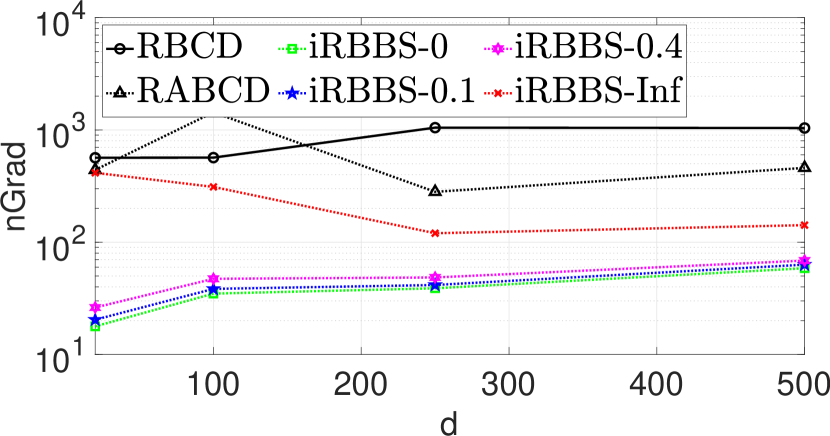
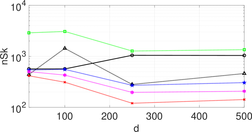
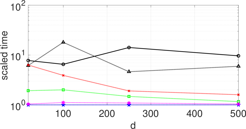
(a) $n=100$

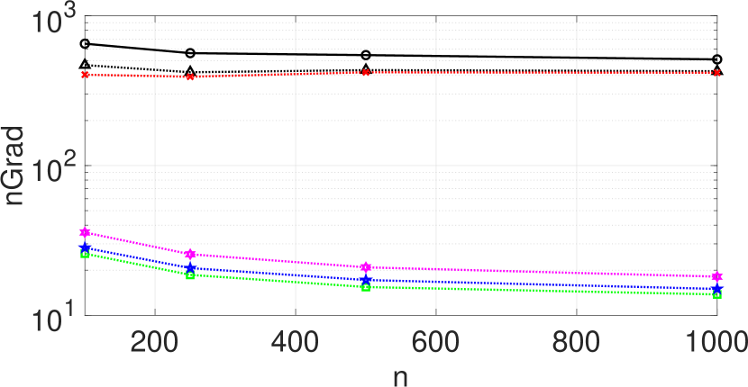
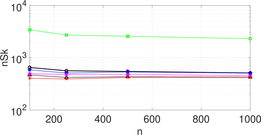
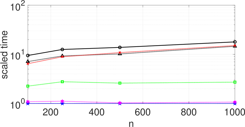
(b) $d=50$

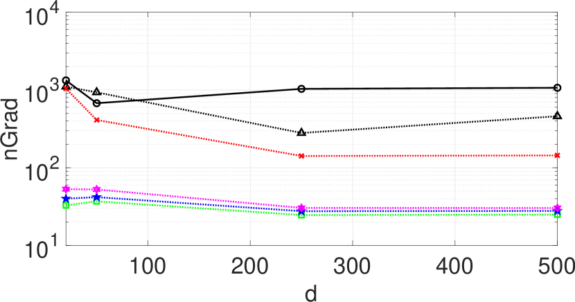
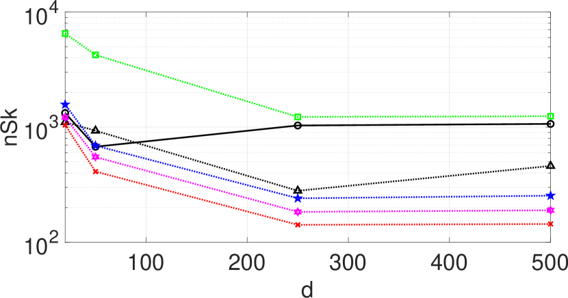
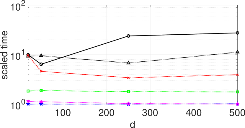
(c) $n=d$

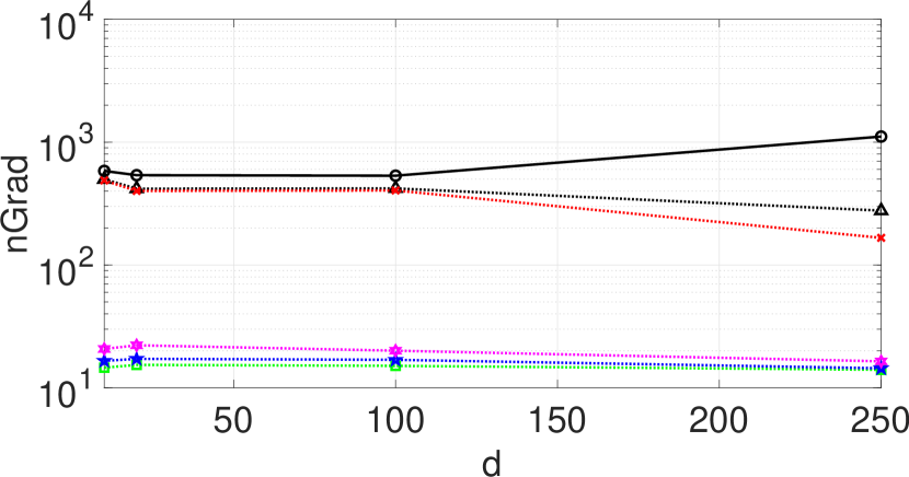
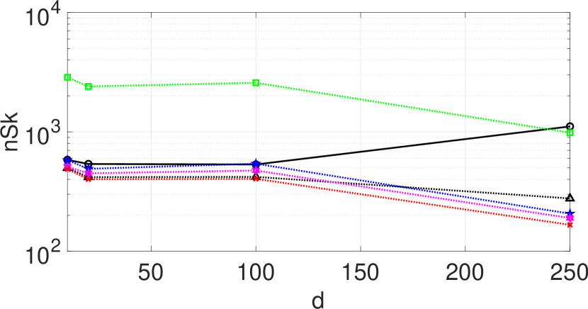
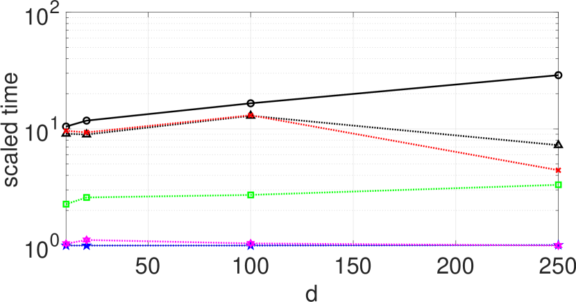
(d) $n=10d$

Figure 1: Results for Section 5. The scaled time means the time of each method over the minimum time of all methods. For (a), $d\in\{20,100,250,500\}$; for (b), $n\in\{100,250,500,1000\}$; for (c), $d\in\{20,50,250,500\}$; for (d), $d\in\{10,20,100,250\}$.

The comparison results for Section 5 are plotted as Fig. 1. Note that the values $\mathrm{PRW_{p}}$ returned by different methods are almost the same for this dataset. Therefore, we do not report the values in the figure. From the figure, we can draw the following observations. i). iRBBS with smaller $\theta$ always has less nGrad but more nSk. This means that computing $\operatorname{grad}q(U^{t})$ in a relatively high precision can help to reduce the whole iteration number of updating $U$. In particular, iRBBS-0, which computes (almost) the exact $\operatorname{grad}q(U^{t})$, takes the least nGrad. Owing to that the complexity of one Sinkhorn iteration is much less than that of updating $U$ (see remarks at the end of section 4.1), iRBBS with a moderate $\theta$ generally achieves the best overall performance. The last rows of Fig. 1 show that iRBBS-0.1 is almost the fastest among all iRBBS methods. ii). Our iRBBS-$\theta$ is better than R(A)BCD in terms that the former ones always have smaller nGrad and nSk and are always faster. Particularly, for Section 5, iRBBS-0.1 is always more than 5x faster than RABCD and is about more than 10x faster than RBCD. For the largest instance $d=250$, $n=2500$, iRBBS-0.1 (1.6s) is more than 7.2x faster than RABCD (11.1s) and about 28.6x faster than RBCD (44.4s). It should be also mentioned that for all 800 problem instances, there are 5/21 instances in total for which RBCD/RABCD meet the maximum iteration numbers and return solutions not satisfying the stopping criteria.

Table 1: The average results of 20 runs for Section 5. In this table, “a”, “b” stand for RBCD and RABCD, respectively; “c”, “d”, and “e” stand for iRBBS-inf, iRBBS-0.1, and iRBBS-0, respectively. For RBCD, RABCD, and iRBBS-inf, nGrad is always equal to nSk.

	$\mathrm{PRW_{p}}$					nGrad/nSk					time
data	a	b	c	d	e	a	b	c	d	e	a	b	c	d	e
H5/H	0.0491	0.0491	0.0491	0.0491	0.0491	871	604	320	64/1296	61/3218	9.6	6.7	3.4	1.2	1.8
H5/JC	0.0596	0.0596	0.0596	0.0596	0.0596	904	497	193	63/1571	60/3047	5.3	2.9	1.2	0.6	0.7
H5/MV	0.0625	0.0625	0.0625	0.0625	0.0625	800	444	118	63/1373	61/2812	5.4	2.9	0.8	0.6	0.8
H5/O	0.0500	0.0500	0.0500	0.0500	0.0500	612	397	129	43/1084	45/2410	4.9	3.2	1.0	0.5	0.7
H5/RJ	0.1802	0.1802	0.1802	0.1802	0.1802	474	440	319	73/1670	69/3041	3.8	3.5	2.4	0.8	1.0
H/JC	0.0501	0.0501	0.0501	0.0572	0.0572	637	523	427	41/1049	42/2020	4.4	3.6	2.9	0.4	0.6
H/MV	0.0384	0.0384	0.0384	0.0384	0.0384	2794	1661	440	117/2045	125/5129	22.9	13.6	3.4	1.2	1.6
H/O	0.0140	0.0140	0.0140	0.0140	0.0140	796	503	212	49/1471	53/3093	7.7	4.7	2.0	0.8	1.2
H/RJ	0.1895	0.1895	0.1895	0.1895	0.1895	360	441	265	46/933	47/1763	3.4	4.2	2.3	0.6	0.8
JC/MV	0.0133	0.0133	0.0133	0.0133	0.0133	1816	975	216	66/1781	65/3742	7.2	3.8	0.9	0.4	0.6
JC/O	0.0098	0.0098	0.0098	0.0098	0.0098	1160	763	101	52/1402	45/2454	6.5	3.5	0.5	0.4	0.5
JC/RJ	0.1103	0.1103	0.1103	0.1103	0.1103	340	332	235	44/1016	53/2536	1.5	1.5	1.1	0.3	0.5
MV/O	0.0101	0.0101	0.0101	0.0101	0.0101	2222	1396	154	90/2448	88/5186	13.2	8.2	0.9	0.8	1.1
MV/RJ	0.1683	0.1683	0.1683	0.1683	0.1683	842	763	632	85/1688	95/4805	5.0	4.5	3.8	0.7	1.1
O/RJ	0.1256	0.1256	0.1256	0.1241	0.1241	376	372	210	55/1070	62/2749	2.5	2.4	1.4	0.5	0.8
AVG	0.0754	0.0754	0.0754	0.0758	0.0758	1000	674	265	63/1460	65/3200	6.89	4.62	1.86	0.66	0.90

Table 2: The average results of 20 runs for Section 5. In this table, “a”, “c”, “d”, and “e” stand for RBCD, iRBBS-inf, iRBBS-0.1, and iRBBS-0, respectively. For RBCD and iRBBS-inf, nGrad is always equal to nSk.

	$10^{-3}\times\mathrm{PRW_{p}}$				nGrad/nSk				time
data	a	c	d	e	a	c	d	e	a	c	d	e
D0/D1	0.9746	0.9746	0.9746	0.9746	519	132	59/506	46/1062	2.7	0.7	0.4	0.4
D0/D2	0.7942	0.7942	0.7942	0.7942	988	187	72/943	74/2655	4.8	1.0	0.5	0.6
D0/D3	1.2021	1.2021	1.2021	1.2021	554	177	64/934	44/1386	2.6	0.8	0.4	0.4
D0/D4	1.2205	1.2205	1.2308	1.2308	912	243	98/998	81/2947	4.1	1.1	0.5	0.6
D0/D5	1.0266	1.0276	1.0266	1.0266	1178	252	89/1402	96/4355	4.8	1.1	0.5	0.8
D0/D6	0.8027	0.8027	0.8027	0.8027	919	186	66/1052	54/2387	4.0	0.8	0.4	0.5
D0/D7	0.8558	0.8558	0.8558	0.8558	601	163	63/747	56/1727	2.7	0.8	0.4	0.4
D0/D8	1.0529	1.0529	1.0529	1.0529	709	185	84/1330	72/3302	3.1	0.8	0.5	0.6
D0/D9	1.0846	1.0846	1.0846	1.0846	698	179	68/1108	55/2436	3.3	0.8	0.4	0.5
D1/D2	0.6647	0.6647	0.6647	0.6647	757	114	55/638	47/1511	4.1	0.6	0.4	0.5
D1/D3	0.8610	0.8610	0.8610	0.8610	1649	230	105/982	71/2065	8.8	1.3	0.7	0.8
D1/D4	0.6666	0.6666	0.6666	0.6666	982	153	65/505	54/1282	5.1	0.8	0.4	0.5
D1/D5	0.8400	0.8400	0.8400	0.8400	3436	540	184/1503	157/3844	15.9	2.4	1.0	1.1
D1/D6	0.7957	0.7957	0.7957	0.7954	2919	331	128/1095	119/3354	15.0	1.7	0.8	1.1
D1/D7	0.5723	0.5723	0.5723	0.5723	961	157	65/525	56/1253	5.2	0.9	0.4	0.5
D1/D8	0.8784	0.8784	0.8784	0.8783	5000	402	200/2001	181/5505	25.8	2.1	1.3	1.6
D1/D9	0.8534	0.8534	0.8534	0.8534	951	168	69/581	58/1321	5.6	1.0	0.6	0.7
D2/D3	0.7188	0.7188	0.7188	0.7188	2070	336	120/1733	100/4897	10.0	1.6	0.8	1.0
D2/D4	1.0684	1.0854	1.0854	1.0854	5000	4602	550/8093	382/16291	24.3	21.4	3.2	3.4
D2/D5	1.0767	1.0767	1.0767	1.0767	1320	272	109/1910	89/3990	5.9	1.2	0.6	0.7
D2/D6	0.8993	0.8993	0.8993	0.8993	1202	245	102/967	87/3205	5.8	1.2	0.6	0.7
D2/D7	0.6950	0.6950	0.6950	0.6950	951	174	67/1156	63/3108	4.7	0.9	0.5	0.8
D2/D8	0.6711	0.6711	0.6711	0.6711	1293	213	72/925	69/3547	6.2	1.0	0.4	0.7
D2/D9	1.0567	1.0567	1.0567	1.0567	1985	284	120/1907	93/3753	9.4	1.3	0.7	0.8
D3/D4	1.1994	1.2003	1.2003	1.2003	5000	312	76/762	69/2523	22.2	1.4	0.4	0.5
D3/D5	0.5817	0.5817	0.5817	0.5817	1187	181	71/793	58/2430	4.8	0.8	0.4	0.5
D3/D6	1.2317	1.2317	1.2317	1.2317	1028	212	82/772	66/2121	4.5	0.9	0.4	0.5
D3/D7	0.7245	0.7245	0.7245	0.7245	1101	202	88/831	776/19184	5.2	0.9	0.5	5.3
D3/D8	0.8798	0.8798	0.8798	0.8798	916	200	84/1113	77/3675	4.0	0.9	0.5	0.7
D3/D9	0.8302	0.8302	0.8302	0.8302	1572	210	72/955	49/2193	7.2	1.0	0.4	0.4
D4/D5	1.0063	1.0063	1.0063	1.0063	936	245	87/863	71/2748	3.9	1.0	0.4	0.5
D4/D6	0.8436	0.8436	0.8436	0.8436	1312	245	96/1102	82/3463	5.9	1.1	0.5	0.7
D4/D7	0.7899	0.7899	0.7899	0.7899	1351	269	96/912	76/2509	6.4	1.2	0.5	0.6
D4/D8	1.0950	1.0982	1.0982	1.0982	5000	213	52/550	52/1930	21.9	0.9	0.3	0.4
D4/D9	0.4892	0.4892	0.4892	0.4892	1997	281	70/1116	54/2610	9.1	1.3	0.4	0.5
D5/D6	0.7170	0.7170	0.7170	0.7170	1335	220	86/891	69/2536	5.4	0.9	0.4	0.5
D5/D7	0.9126	0.9126	0.9126	0.9126	899	242	72/652	71/2132	3.7	1.0	0.4	0.5
D5/D8	0.7152	0.7152	0.7152	0.7152	1429	225	71/1060	50/2347	5.9	0.9	0.4	0.4
D5/D9	0.7755	0.7755	0.7755	0.7755	1413	252	86/1216	64/3451	5.9	1.0	0.5	0.6
D6/D7	1.1098	1.1098	1.1098	1.1098	826	195	66/398	62/1318	3.8	0.9	0.3	0.4
D6/D8	0.9175	0.9175	0.9175	0.9175	725	186	57/721	57/2305	3.2	0.8	0.3	0.5
D6/D9	1.1055	1.1055	1.1055	1.1055	1117	219	95/1038	79/3046	5.0	1.0	0.5	0.6
D7/D8	1.0787	1.0787	1.0787	1.0787	757	180	68/796	59/2455	3.5	0.8	0.4	0.5
D7/D9	0.6079	0.6079	0.6079	0.6079	1985	266	79/1026	72/3208	9.3	1.3	0.5	0.7
D8/D9	0.8678	0.8678	0.8678	0.8678	745	180	57/713	50/2107	3.2	0.8	0.3	0.4
AVG	0.8847	0.8852	0.8854	0.8854	1560	326	95/1152	95/3366	7.28	1.52	0.57	0.78

The comparison results for Sections 5 and 5 are reported in Tables 1 and 2, respectively. In the last “AVG” line, we summarize the averaged “$\mathrm{PRW_{p}}$”, “nGrad/nSk” and “time”. From the tables, we have the following observations. i). As for the solution quality, iRBBS-0 and iRBBS-0.1 perform the best among all methods. ii). Among iRBBS methods, iRBBS-0.1 and iRBBS-0 take the least nGrad and iRBBS-inf takes the most nGrad while iRBBS-0 takes the most nSk and iRBBS-inf takes the least nSk. Compared with iRBBS-inf, iRBBS-0.1 is about 2.8x faster for Section 5 and is about 2.7x faster for Section 5. Compared with iRBBS-0, iRBBS-0.1 is about 1.4x faster for Sections 5 and 5. iii). Compared with R(A)BCD, iRBBS-0.1 can always take significantly less nGrad and may take a bit more nSk. This makes it about 7x faster than RABCD and about 10.4x faster than RBCD for Section 5, and about 12.8x faster than RBCD for Section 5. Besides, for instances D1/D8, D2/D4, D3/D4, D4/D8, RBCD meets the maximum iteration number.

We now further investigate the benefit of performing several Sinkhorn iterations over only performing one Sinkhorn iteration in each update of the variable $U$. The results of iRBBS-inf and iRBBS-0.1 for different values of $\eta$, as well as the results of RABCD with $\eta=0.1$ for Section 5 and RBCD with $\eta=8$ for Section 5, are plotted as Fig. 2. From this figure, we can make the following observations. i) Our method iRBBS with different $\theta$ for solving (25) with a smaller $\eta$ is still much better than R(A)BCD for solving (25) with a larger $\eta$ in terms of both speed and solution quality. Specifically, for $\eta=0.05$, our iRBBS-0.1 is still about 4.6x faster for Section 5 and the returned $\mathrm{PRW}_{p}$ (0.0918) is 1.2x better than that of RABCD (0.0754). For $\eta=3$, our iRBBS-0.1 is still about 11.5x faster than RBCD for Section 5, and the returned $\mathrm{PRW}_{p}$ (886.1) is better than that of RBCD (884.7). ii) Generally, problem (25) with a smaller $\eta$ can return better solutions but is harder to solve. The strategy of doing several Sinkhorn iterations while updating $U$ once can indeed speed up the algorithm for different $\eta$ and the advantage of iRBBS-0.1 over iRBBS-inf is larger for smaller $\eta$.

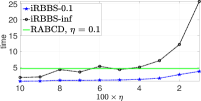
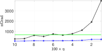
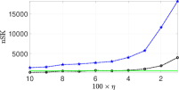
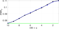
(a)

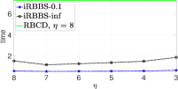
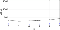
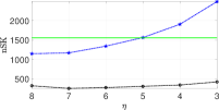
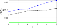
(b)

Figure 2: Comparison of iRBBS-inf and iRBBS-0.1 for different $\eta$. The top four figures are for Section 5 and the bottom four figures are for Section 5.

From the above results, we can conclude that iRBBS generally perform much better than R(A)BCD for the three datasets. More importantly, our methods adopt the adaptive stepsize without needing to tune the best stepsize as done in R(A)BCD.

5.2 Comparison on computing the PRW distance (1)

In this subsection, we present numerical results to illustrate the effectiveness and efficiency of our proposed ReALM algorithm, namely, Algorithm 1. The subproblem (13) is solved by our developed iRBBS algorithm, namely, Algorithm 2, with $\theta_{t}$ chosen via (62).

Parameters of ReALM. In our numerical tests, we choose $\epsilon_{1}=2\|C\|_{\infty}\epsilon_{2}$, $\epsilon_{2}=10^{-6}\max\{\|r\|_{\infty},\|c\|_{\infty}\}$, and $\epsilon_{c}=10^{-5}$. To prevent too small $\eta$, in our implementation, we update $\eta_{k+1}=\min\left\{\gamma_{\eta}\eta_{k},\eta_{\min}\right\}$ other than using (17), where $\eta_{\min}$ is a preset positive number. Once $\eta_{k}$ becomes $\eta_{\min}$, we set the corresponding $\epsilon_{k,1}=\epsilon_{1}$ and $\epsilon_{k,2}=\epsilon_{2}$ and stop the algorithm if $\mathsf{e}_{1}(\mathbf{x}^{k},\pi^{k})\leq\epsilon_{1}$ and $\mathsf{e}_{2}(\mathbf{x}^{k},\pi^{k})\leq\epsilon_{2}$. To avoid possible numerical instability, we restrict the maximum number of updating $\pi^{k}$ as 8. We set $\gamma_{\epsilon}=0.25$ and choose $\epsilon_{1,2}=10^{-1}\max\{\|r\|_{\infty},\|c\|_{\infty}\}$ and $\epsilon_{1,1}=2\|C\|_{\infty}\epsilon_{1,2}$. The initial point is chosen according to the way in section 5.1. Moreover, we denote by ReALM-$(\eta_{\min},\gamma_{W})$ the ReALM algorithm with particular parameters $\eta_{\min}$ and $\gamma_{W}$. Note that choosing $\gamma_{W}=0$ means that we adopt a continuation technique to solve the problem (13) with $\pi^{k}\equiv\pi^{1}$ and $\eta_{k}=\eta_{\min}$, which is generally better than directly solving a single problem (13) with a small $\eta_{k}=\eta_{\min}$.

Parameters of iRBBS in ReALM. If $\max\{\|r\|_{\infty},\|c\|_{\infty}\}/\eta_{k}\geq 500$ or $\|C(U^{t})-\eta_{k}\log\pi^{k}\|_{\mathrm{var}}/\eta_{k}$$\geq 900$, we perform the Sinkhorn iteration (41) and set $\theta=10$ in (62); otherwise, we perform the Sinkhorn iteration (42) and set $\theta=0.1$ in (62).

Table 3: The average results for Section 5. In this table, “a” and “b” stand for ReALM-$(0.02,0)$ and ReALM-$(0.055,0.9)$, respectively.

	$\mathrm{PRW_{p}}$		nGrad		$\mbox{nSk}_{\exp}$/$\mbox{nSk}_{\log}$		time		iter
$n$/$d$	a	b	a	b	a	b	a	b	a	b
100/20	8.3430	8.3430	182	138	3208/8342	13258/0	1.1	0.1	0.0/7.0	8.0/14.0
100/100	9.1732	9.1734	287	241	3837/3354	11369/0	0.5	0.1	0.0/7.0	8.0/14.0
100/250	10.8956	10.8969	467	348	3200/8858	10550/279	1.3	0.2	0.0/7.0	8.0/14.1
100/500	13.3111	13.3152	680	469	2192/3782	9844/213	0.8	0.2	0.0/7.0	8.0/14.0
100/50	8.5999	8.6000	321	189	3945/13096	11700/0	1.8	0.1	0.0/7.0	8.0/14.0
250/50	8.2334	8.2334	150	156	2480/4168	10828/0	2.2	0.3	0.0/7.0	7.9/13.9
500/50	8.1299	8.1299	122	141	1944/4508	11578/0	7.2	0.8	0.0/7.0	8.0/14.0
1000/50	8.0710	8.0709	111	130	1716/5307	12344/0	30.8	2.3	0.0/7.0	8.0/14.0
20/20	9.3098	9.3104	591	221	4016/23861	11906/0	0.5	0.0	0.0/7.1	8.0/14.0
50/50	9.3627	9.3629	386	248	4656/9416	11819/0	0.5	0.1	0.0/7.0	7.9/13.9
250/250	9.1744	9.1748	282	257	2942/4136	11371/248	2.2	0.5	0.0/7.0	8.0/14.0
500/500	9.1150	9.1154	258	262	2391/4884	9927/873	7.5	2.2	0.0/7.0	7.6/13.6
100/10	8.1620	8.1619	405	173	4635/33570	65772/0	4.6	0.3	0.0/7.0	8.0/14.0
200/20	8.1331	8.1331	180	128	2861/10259	15007/0	3.8	0.3	0.0/7.0	8.0/14.0
1000/100	8.1187	8.1187	124	145	2096/5157	12153/141	30.5	3.1	0.0/7.0	8.0/14.0
2500/250	8.1164	8.1164	117	146	2416/5499	11482/624	373.8	103.3	0.0/7.0	7.9/13.9
AVG	9.0156	9.0160	291	212	3033/9262	15057/149	29.3	7.1	0.0/7.0	8.0/14.0

The results for Section 5 are presented in Table 3. In this table and the subsequent tables, the terms “$\mbox{nSk}_{\log}$” and “$\mbox{nSk}_{\exp}$” mean the total numbers of Sinkhorn iterations (41) and (42), respectively, the pair “$K_{1}$/$K$” in the column “iter” means that the corresponding algorithm stops at the $K$-iteration and updates the multiplier matrix $K_{1}$ times. For each $(n,d)$ pair, we randomly generate 10 instances, each equipped with 5 randomly generated initial points. We conside ReALM-$(0.055,0.9)$ and ReALM-$(0.02,0)$ both with $\eta_{1}=1$ and $\gamma_{\eta}=0.5$. Note that the latter admits a smaller $\eta_{\min}$ and does not update the multiplier matrix. From Table 3, we can observe that ReALM-$(0.055,0.9)$ can not only return better solutions than ReALM-$(0.02,0.9)$ but also is about 4x faster. This shows that updating the multiplier matrix does help. In fact, on average ReALM-$(0.055,0.9)$ updates the multiplier matrix 8 times in 14 total iterations. The reasons why ReALM with updating the multiplier matrix outperforms ReALM without updating the multiplier matrix in terms of solution quality and speed are as follows. First, updating the multiplier matrix in ReALM can keep the solution quality even using a larger $\eta$. Second, solving the subproblem with a larger $\eta$ is always easier, which enables that ReALM-$(0.055,0.9)$ computes less $\operatorname{grad}\mathcal{L}(\mathbf{x})$ and performs less Sinkhorn iterations (41) which involves computing the log-sum-exp function $\log\sum_{i}\exp(x_{i}/\eta)=x_{\max}/\eta+\log\sum_{i}\exp(x_{i}/\eta-x_{\max}/\eta)$ for small $\eta$.

Table 4: The average results for Sections 5 and 5. For Section 5, $\Gamma=1$, “a” and “b” stand for ReALM-$(0.0035,0)$ and ReALM-$(0.07,0.9)$, respectively. For Section 5, $\Gamma=10^{-3}$, “a” and “b” stand for ReALM-$(1,0)$ and ReALM-$(3,0.9)$, respectively.

	$\Gamma\times\mathrm{PRW_{p}}$		nGrad		$\mbox{nSk}_{\exp}$/$\mbox{nSk}_{\log}$		time		iter
data	a	b	a	b	a	b	a	b	a	b
H5/JC	0.0927	0.1099	1081	675	23809/8267	9786/0	84.1	8.6	0.0/8.0	8.0/15.0
H/MV	0.0638	0.0642	1116	727	3864/13382	30997/0	175.7	14.9	0.0/8.0	8.0/15.0
H/RJ	0.2171	0.2261	547	788	3091/4062	11747/0	63.3	15.6	0.0/8.0	8.0/15.0
JC/MV	0.0627	0.0623	1324	711	12875/9727	17073/0	55.3	5.9	0.0/8.0	8.0/15.0
JC/O	0.0422	0.0428	1650	1100	4997/26612	35031/4500	204.7	46.7	0.0/8.0	8.0/15.0
MV/O	0.0418	0.0366	890	822	6101/5289	31651/0	57.0	13.3	0.0/8.0	8.0/15.0
AVG	0.1134	0.1146	863	787	7824/7364	20261/300	78.0	15.0	0.0/8.0	8.0/15.0
D0/D4	1.2210	1.2316	428	632	2169/3599	6564/0	20.8	4.8	0.0/5.0	8.0/13.0
D2/D5	1.0771	1.0861	574	1083	707/6040	7035/1642	33.0	15.0	0.0/5.0	8.0/13.0
D2/D7	0.6955	0.7012	272	538	1890/2284	7972/0	21.0	6.0	0.0/5.0	7.0/12.0
D2/D9	1.0570	1.0697	502	721	3027/4541	4172/0	28.0	5.9	0.0/5.0	8.0/13.0
AVG	0.8861	0.8870	386	783	1504/2378	9551/36	16.1	6.7	0.0/5.0	6.7/11.7

The results over 20 runs on the real datasets Sections 5 and 5 are reported in Table 4. We choose $\eta_{1}=20$ for Section 5 and $\eta_{1}=200$ for Section 5 and set $\gamma_{\eta}=0.25$ for both datasets. To save space, we only report instances where one method can return the value “$\mathrm{PRW_{p}}$” larger than 1.005 times of the smaller one of the two $\mathrm{PRW_{p}}$ values returned by the two methods. The better “$\mathrm{PRW_{p}}$” is marked in bold . Besides, the average performance over all instances (15 instances in total for Section 5 and 45 instances in total for Section 5) for each dataset is also kept in the “AVG” line. From this table, we can see that updating the multiplier matrix also helps for the two real datasets. Compared with ReALM without updating the multiplier, ReALM with updating the multiplier can not only return better solutions but is about 5.2x faster for Section 5 and is about 2.4x faster for Section 5.

6 Concluding remarks

In this paper, we considered the computation of the PRW distance arising from machine learning applications. By reformulating this problem as an optimization problem over the Cartesian product of the Stiefel manifold and the Euclidean space with additional nonlinear inequality constraints, we proposed a ReALM method. The convergence of ReALM was also established. To solve the subproblem in the ReALM method, we developed a framework of inexact Riemannian gradient descent methods. Also, we provided a practical iRBBS method with convergence and complexity guarantees, wherein the Riemannian BB stepsize and Sinkhorn iterations are employed. Our numerical results showed that, compared with the state-of-the-art methods, our proposed ReALM and iRBBS methods both have advantages in solution quality and speed. Moreover, our proposed ReALM method can be also extended to solve more general Riemannian optimization with additional inequality constraints.

References

• [1] P.-A. Absil, R. Mahony, and R. Sepulchre, Optimization algorithms on matrix manifolds, in Optimization Algorithms on Matrix Manifolds, Princeton University Press, 2009.
• [2] J. Altschuler, J. Niles-Weed, and P. Rigollet, Near-linear time approximation algorithms for optimal transport via Sinkhorn iteration, Adv. Neural Inf. Process. Syst., 30 (2017).
• [3] R. Andreani, E. G. Birgin, J. M. Martínez, and M. L. Schuverdt, On augmented Lagrangian methods with general lower-level constraints, SIAM J. Optim., 18 (2008), pp. 1286–1309.
• [4] J. Barzilai and J. M. Borwein, Two-point step size gradient methods, IMA J. Numer. Anal., 8 (1988), pp. 141–148.
• [5] A. S. Berahas, L. Cao, and K. Scheinberg, Global convergence rate analysis of a generic line search algorithm with noise, SIAM J. Optim., 31 (2021), pp. 1489–1518.
• [6] D. P. Bertsekas, Constrained optimization and Lagrange multiplier methods, Academic Press, 2014.
• [7] S. Bonettini, Inexact block coordinate descent methods with application to non-negative matrix factorization, IMA J. Numer. Anal., 31 (2011), pp. 1431–1452.
• [8] N. Boumal, An introduction to optimization on smooth manifolds, Available online, May, 3 (2020).
• [9] N. Boumal, P.-A. Absil, and C. Cartis, Global rates of convergence for nonconvex optimization on manifolds, IMA J. Numer. Anal., 39 (2019), pp. 1–33.
• [10] R. G. Carter, On the global convergence of trust region algorithms using inexact gradient information, SIAM J. Numer. Anal., 28 (1991), pp. 251–265.
• [11] A. Chambolle and J. P. Contreras, Accelerated Bregman primal-dual methods applied to optimal transport and Wasserstein barycenter problems, arXiv:2203.00802, (2022).
• [12] M. Cuturi, Sinkhorn distances: Lightspeed computation of optimal transport, Adv. Neural Inf. Process. Syst., 26 (2013).
• [13] O. Devolder, F. Glineur, and Y. Nesterov, First-order methods of smooth convex optimization with inexact oracle, Math. Program., 146 (2014), pp. 37–75.
• [14] M. Doljansky and M. Teboulle, An interior proximal algorithm and the exponential multiplier method for semidefinite programming, SIAM J. Optim., 9 (1998), pp. 1–13.
• [15] P. Dvurechensky, A. Gasnikov, and A. Kroshnin, Computational optimal transport: Complexity by accelerated gradient descent is better than by Sinkhorn’s algorithm, in ICML, PMLR, 2018, pp. 1367–1376.
• [16] N. Echebest, M. D. Sánchez, and M. L. Schuverdt, Convergence results of an augmented Lagrangian method using the exponential penalty function, J. Optim. Theory Appl., 168 (2016), pp. 92–108.
• [17] A. Edelman, T. A. Arias, and S. T. Smith, The geometry of algorithms with orthogonality constraints, SIAM J. Matrix Anal. Appl., 20 (1998), pp. 303–353.
• [18] N. Fournier and A. Guillin, On the rate of convergence in Wasserstein distance of the empirical measure, Probab. Theory Relat. Fields, 162 (2015), pp. 707–738.
• [19] B. Gao, X. Liu, X. Chen, and Y.-x. Yuan, A new first-order algorithmic framework for optimization problems with orthogonality constraints, SIAM J. Optim., 28 (2018), pp. 302–332.
• [20] E. Gur, S. Sabach, and S. Shtern, Convergent nested alternating minimization algorithms for nonconvex optimization problems, Math. Oper. Res., (2022).
• [21] Y.-Q. Hu and Y.-H. Dai, Inexact Barzilai-Borwein method for saddle point problems, Numer. Linear Algebr., 14 (2007), pp. 299–317.
• [22] M. Huang, S. Ma, and L. Lai, A Riemannian block coordinate descent method for computing the projection robust Wasserstein distance, in ICML, PMLR, 2021, pp. 4446–4455.
• [23] Y.-K. Huang, Y.-H. Dai, and X.-W. Liu, Equipping the Barzilai–Borwein method with the two dimensional quadratic termination property, SIAM J. Optim., 31 (2021), pp. 3068–3096.
• [24] B. Iannazzo and M. Porcelli, The Riemannian Barzilai–Borwein method with nonmonotone line search and the matrix geometric mean computation, IMA J. Numer. Anal., 38 (2018), pp. 495–517.
• [25] B. Jiang and Y.-H. Dai, A framework of constraint preserving update schemes for optimization on Stiefel manifold, Math. Program., 153 (2015), pp. 535–575.
• [26] S. Kullback, A lower bound for discrimination information in terms of variation (corresp.), IEEE Trans. Inf. Theory, 13 (1967), pp. 126–127.
• [27] X. Li, An aggregate function method for nonlinear programming, Sci. China Ser. A., 34 (1991), pp. 1467–1473.
• [28] X. Li, S. Chen, Z. Deng, Q. Qu, Z. Zhu, and A. M.-C. So, Weakly convex optimization over Stiefel manifold using Riemannian subgradient-type methods, SIAM J. Optim., 31 (2021), pp. 1605–1634.
• [29] T. Lin, C. Fan, N. Ho, M. Cuturi, and M. Jordan, Projection robust Wasserstein distance and Riemannian optimization, Adv. Neural Inf. Process. Syst., 33 (2020), pp. 9383–9397.
• [30] T. Lin, N. Ho, and M. I. Jordan, On the efficiency of entropic regularized algorithms for optimal transport, J. Mach. Learn. Res., 23 (2022), pp. 1–42.
• [31] T. Lin, Z. Zheng, E. Chen, M. Cuturi, and M. I. Jordan, On projection robust optimal transport: Sample complexity and model misspecification, in AISTATS, PMLR, 2021, pp. 262–270.
• [32] H. Liu, A. M.-C. So, and W. Wu, Quadratic optimization with orthogonality constraint: Explicit Łojasiewicz exponent and linear convergence of retraction-based line-search and stochastic variance-reduced gradient methods, Math. Program., 178 (2019), pp. 215–262.
• [33] Z. Lu and Y. Zhang, An augmented Lagrangian approach for sparse principal component analysis, Math. Program., 135 (2012), pp. 149–193.
• [34] J. Niles-Weed and P. Rigollet, Estimation of Wasserstein distances in the spiked transport model, arXiv:1909.07513, (2019).
• [35] F.-P. Paty and M. Cuturi, Subspace robust Wasserstein distances, in ICML, PMLR, 2019, pp. 5072–5081.
• [36] G. Peyré and M. Cuturi, Computational optimal transport: With applications to data science, Foundations and Trends® in Machine Learning, 11 (2019), pp. 355–607.
• [37] E. W. Sachs and S. M. Sachs, Nonmonotone line searches for optimization algorithms, Control Cybern., 40 (2011), pp. 1059–1075.
• [38] H.-J. M. Shi, Y. Xie, R. Byrd, and J. Nocedal, A noise-tolerant quasi-Newton algorithm for unconstrained optimization, SIAM J. Optim., 32 (2022), pp. 29–55.
• [39] E. Torrealba, L. Matioli, M. Nasri, and R. Castillo, Exponential augmented Lagrangian methods for equilibrium problems, Optim. Method Softw., (2020), pp. 1–25.
• [40] P. Tseng and D. P. Bertsekas, On the convergence of the exponential multiplier method for convex programming, Math. Program., 60 (1993), pp. 1–19.
• [41] J.-P. Vial, Strong and weak convexity of sets and functions, Math. Oper. Res., 8 (1983), pp. 231–259.
• [42] J. Weed and F. Bach, Sharp asymptotic and finite-sample rates of convergence of empirical measures in Wasserstein distance, Bernoulli, 25 (2019), pp. 2620–2648.
• [43] Z. Wen and W. Yin, A feasible method for optimization with orthogonality constraints, Math. Program., 142 (2013), pp. 397–434.
• [44] Y. Xie, X. Wang, R. Wang, and H. Zha, A fast proximal point method for computing exact Wasserstein distance, in Uncertainty in Artificial Intelligence, PMLR, 2020, pp. 433–453.
• [45] L. Yang and K.-C. Toh, Bregman proximal point algorithm revisited: A new inexact version and its variant, SIAM J. Optim., 32 (2022), pp. 1523–1554.
• [46] W. H. Yang, L.-H. Zhang, and R. Song, Optimality conditions for the nonlinear programming problems on Riemannian manifolds, Pac. J. Optim., 10 (2014), pp. 415–434.
• [47] H. Zhang and W. W. Hager, A nonmonotone line search technique and its application to unconstrained optimization, SIAM J. Optim., 14 (2004), pp. 1043–1056.