Propulsive performance of oscillating plates with time-periodic flexibility

Abstract

We use small-amplitude inviscid theory to study the swimming performance of a flexible flapping plate with time-varying flexibility. The stiffness of the plate oscillates at twice the frequency of the kinematics in order to maintain a symmetric motion. Plates with constant and time-periodic stiffness are compared over a range of mean plate stiffness, oscillating stiffness amplitude, and oscillating stiffness phase for isolated heaving, isolated pitching, and combined leading edge kinematics. We find that there is a profound impact of oscillating stiffness on the thrust, with a lesser impact on propulsive efficiency. Thrust improvements of up to 35% relative to a constant-stiffness plate are observed. For large enough frequencies and amplitudes of the stiffness oscillation, instabilities emerge. The unstable regions may confer enhanced propulsive performance; this hypothesis must be verified via experiments or nonlinear simulations.

1 Introduction

For decades research has focused on studying the fluid dynamics of biological swimmers, both to better understand the underlying biology of aquatic animals, and to provide inspiration for developing innovative hydrodynamic propulsion technology (Smits, 2019). A salient feature of natural swimmers is the action of muscles, which are often distributed throughout an animal’s propulsor (Flammang & Lauder, 2008; Adams & Fish, 2019). Through observations and measurements of animals, we know that swimmers can control their fin curvature, displacement, and area as well as their stiffness (Fish & Lauder, 2006). It stands to reason that swimmers may be able to utilize their muscles on the time scale of the oscillation of their propulsors to tune performance, e.g., by dynamically changing the stiffness of their propulsors; however, there is no definitive observation or consensus in the biological community that swimmers take advantage of their muscles in this way (Fish & Lauder, 2021). In this work we will show that, from a purely hydrodynamic perspective, time-varying stiffness leads to propulsive benefits over constant-stiffness propulsors.

The fluid dynamics of biological swimmers is rooted in the theory of rigid-wing flutter. Theodorsen (1935) was first to theoretically model the forces produced by oscillating foils in a fluid, which was later extended by Garrick (1936) to analytically predict thrust and power for a rigid oscillating foil. Although these works focused on wing flutter, the connection to swimmers was clear. Later, Chopra & Kambe (1977) incorporated the effects of three-dimensionality via lifting line theory. Anderson et al. (1998) used particle image velocimetry to calculate thrust and power of harmonically oscillating foils and compared the results to inviscid theory predictions. More recently, Floryan et al. (2017a) derived and experimentally validated propulsive scaling laws for rigid two-dimensional foils in pure heaving and pitching motions. This was extended to combined pitch-and-heave motions (Van Buren et al., 2019) and non-sinusoidal motions (Van Buren et al., 2017; Floryan et al., 2017b).

The passive flexibility (or elasticity) of an oscillating propulsor plays a key role in its propulsive performance. In a particularly influential work, Wu (1961) was one of the first to analytically consider passive flexibility, albeit through prescribed kinematics. Katz & Weihs (1978, 1979) calculated the coupled fluid-structure interactions for a two-dimensional flexible foil. Since then, many analytical, experimental, and computational studies have shown the influence of propulsor flexibility on characteristics like thrust and swimming efficiency, generally finding that flexibility can dramatically increase thrust and/or efficiency compared to a rigid propulsor (Alben, 2008; Michelin & Llewellyn Smith, 2009; Dewey et al., 2013; Quinn et al., 2014; Paraz et al., 2016; Moore, 2014, 2015). In a particularly relevant work, Floryan & Rowley (2018) used small-amplitude theory to explore the role of resonance in constant-stiffness propulsors, finding that the benefits of resonance manifest in the thrust and power, but not necessarily in the propulsive efficiency. This analysis was extended in Goza et al. (2020) to consider the role of nonlinearity in the fluid-structure system.

Few works have explored beyond simple uniform and passive flexibility. Floryan & Rowley (2020) considered the role of stiffness distribution, finding that concentrating stiffness toward the leading edge produced higher thrust, but lower efficiency compared to foils with stiffness concentrated away from the leading edge. Quinn & Lauder (2021) studied tuneable stiffness—that is, quasi-steady changes in stiffness—where it was shown that stiffness could be tuned to maximize desired performance parameters. To our knowledge, the only work that considers time-varying stiffness at the same time scale as the kinematics is Shi et al. (2020) and Hu et al. (2021). The former used a finite-volume Navier-Stokes solver to study the effects of changing the flexibility of a nonlinear beam in the context of micro-air-vehicles, and the latter approximated a flexible plate by a rigid propulsor with a torsional spring at its leading edge heaving actively and pitching passively, respectively. By changing the stiffness of the torsional spring in time, Hu et al. (2021) found that both the thrust and propulsive efficiency could be enhanced in swimming. Shi et al. (2020) finds there can be an increase in thrust of up to $52\%$, with little impact on efficiency.

In this work, we study the effects of time-periodic stiffness on the propulsive performance of a flexible plate. We solve a potential flow model that strongly couples the fluid and structural equations of motion. We use a pseudospectral method developed in Moore (2017) to solve the equations of motion, introducing time-varying flexibility through a Fourier series expansion in time. This fast solver allows us to explore the propulsive performance over a large range of parameters. We then use Floquet theory to assess the stability of the system. We will show that the oscillating stiffness can strongly influence thrust and and weakly influence the efficiency of the oscillating propulsor, indicating that animals or human-made swimmers would benefit from this capability.

2 Problem statement and solution methods

Consider a two-dimensional, inextensible plate in a fluid flow, as sketched in Figure 1. The plate has thickness $d$ and length $L$, and we assume that it is thin ($d\ll L$) and that its maximum deflection is small, with its slope $|Y_{x}|\ll 1$. The deflection of the plate is then governed by the Euler-Bernoulli beam equation,

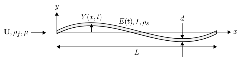
Figure 1: A two-dimensional flat plate with time-varying Young’s modulus moving through a fluid.

$$\rho_{s}dwY_{tt}+E(t)IY_{xxxx}=w\Delta p,$$ (1)

where $Y$ is the transverse displacement of the plate, $\rho_{s}$ is its density, $E(t)$ is its time-varying Young’s modulus, $I=wd^{3}/12$ is its second moment of area, and $w$ is its width. The plate is immersed in a fluid which imparts a hydrodynamic load onto it, given by the pressure difference across the plate, $\Delta p$. Subscript $t$ denotes differentiation with respect to time, and subscript $x$ denotes differentiation with respect to the streamwise coordinate.

The fluid is inviscid and incompressible, with density $\rho_{f}$. Far from the plate, the fluid moves with a freestream velocity $\boldsymbol{U}=U\boldsymbol{i}$, where $\boldsymbol{i}$ is the unit vector in the $x$ direction. Conservation of mass and momentum for the fluid lead to

$$\boldsymbol{\nabla}\cdot\boldsymbol{u}=0,$$ (2a)

$$\rho_{f}(\boldsymbol{u}_{t}+U\boldsymbol{u}_{x})=-\boldsymbol{\nabla}p,$$ (2b)

where $\boldsymbol{u}=u\boldsymbol{i}+v\boldsymbol{j}$ is the perturbation velocity induced by the motion of the plate, and $\boldsymbol{j}$ is the unit vector in the transverse direction. In obtaining (2b), we have assumed that $|\boldsymbol{u}|\ll U$, which is consistent with our assumption of small-amplitude deflections of the plate.

We nondimensionalize the equations of motion using the half-length of the plate $L/2$ as the length scale, the freestream velocity $U$ as the velocity scale, and the convective time $L/(2U)$ as the time scale. The nondimensional equation for the plate is

$$2RY_{tt}+\frac{2}{3}S(t)Y_{xxxx}=\Delta p,$$ (3)

and the nondimensional equations for the fluid are

$$\boldsymbol{\nabla}\cdot\boldsymbol{u}=0,$$ (4a)

$$\boldsymbol{u}_{t}+\boldsymbol{u}_{x}=\boldsymbol{\nabla}\phi,$$ (4b)

where

$$R=\frac{\rho_{s}d}{\rho_{f}L},\;\;\;S(t)=\frac{E(t)d^{3}}{\rho_{f}U^{2}L^{3}},\;\;\;\phi=p_{\infty}-p.$$ (5)

The function $\phi$ is Prandtl’s acceleration potential (Wu, 1961). Now $x$, $t$, $Y$, $\boldsymbol{u}$, and $p$ are nondimensional, with $x=-1$ corresponding to the leading edge of the plate, and $x=1$ corresponding to the trailing edge. The mass ratio $R$ is the ratio of a characteristic mass of the plate to a characteristic mass of fluid, and the stiffness ratio $S$ is the ratio of a characteristic bending force to a characteristic fluid force. The stiffness ratio, its inverse, and variations of it are sometimes called the Cauchy number (de Langre, 2008) or the elastohydrodynamical number (Schouveiler & Boudaoud, 2006).

To close the system of equations, we specify the boundary conditions. The fluid satisfies the no-penetration boundary condition and the Kutta condition,

$$v|_{x\in[-1,1],y=0}=Y_{t}+Y_{x},$$ (6a)

$$|v||_{(x,y)=(1,0)}<\infty.$$ (6b)

We specify heaving and pitching motions $h$ and $\theta$, respectively, at the leading edge of the plate, while the trailing edge is free (zero force and torque), resulting in the boundary conditions

$$Y(-1,t)=h(t),\;\;\;Y_{x}(-1,t)=\theta(t),\;\;\;Y_{xx}(1,t)=0,\;\;\;Y_{xxx}(1,t)=0.$$ (7)

Since we are interested in locomotion, we consider periodic actuation of the leading edge; that is, $h(t)$ and $\theta(t)$ are (zero-mean) periodic functions of $t$ with a nondimensional angular frequency $\sigma=\pi fL/U$, where $f$ is the dimensional ordinary frequency. Similarly, we consider a time-periodic stiffness. With our focus on forward propulsion, the upstroke and downstroke must be mirror images of each other in order for the mean side force to be zero. It can be shown that this requires that the stiffness vary at twice the frequency of the deflection of the plate. Intuitively, the stiffness must be the same during the upstroke and downstroke, which can only be true if it varies at twice the frequency of the plate’s deflection.

To solve the system of equations for the kinematics of the plate, we use the method described by Moore (2017), adapting it to account for time-periodic stiffness; we describe the method in Appendix A. The method assumes that the kinematics are time-periodic, with any transients decaying to zero. We will test this assumption by performing a Floquet analysis. More importantly, the Floquet analysis will provide physical insight into the problem. The Floquet analysis is adapted from the eigenvalue problem described by Floryan & Rowley (2018, 2020) and uses a key idea from Kumar & Tuckerman (1994); the details are in Appendix B.

The motion of the plate induces a pressure difference across it. The projection of the pressure difference onto the horizontal direction contributes—together with a suction force at the leading edge—to a propulsive thrust force. Therefore, the energy put into the system by actuating the leading edge is converted into propulsive thrust, given by

$$C_{T}=\int_{-1}^{1}\Delta pY_{x}dx+C_{TS},$$ (8)

where $C_{TS}$ is the leading edge suction, a formula for which is given by Moore (2017). The power input is

$$C_{P}=-\int_{-1}^{1}\Delta pY_{t}dx.$$ (9)

Finally, the Froude efficiency is defined as the ratio of the time-averaged thrust output to the time-averaged power input (i.e., how much of the power input is converted to propulsive thrust),

$$\eta=\frac{\overline{C_{T}}}{\overline{C_{P}}},$$ (10)

where the overbar denotes averaging in time.

In this work, we restrict ourselves to leading edge actuation and stiffnesses that are sinusoidal in time,

$$h(t) =\frac{1}{2}\left(h_{0}e^{j\sigma t}+h_{0}^{*}e^{-j\sigma t}\right),$$ (11a)

$$\theta(t) =\frac{1}{2}\left(\theta_{0}e^{j\sigma t}+\theta_{0}^{*}e^{-j\sigma t}\right),$$ (11b)

$$S(t) =\overline{S}+\frac{\overline{S}}{2}\left(S_{0}e^{2j\sigma t}+S_{0}^{*}e^{-2j\sigma t}\right),$$ (11c)

where $h_{0},\theta_{0},S_{0}\in\mathbb{C}$, $j=\sqrt{-1}$, and a superscript $*$ denotes complex conjugation. The formulation in the appendices, however, is valid for generic smooth periodic functions of time. We will make frequent use of the parameter $\phi_{S}=\text{arg}(S_{0})$, the phase of the stiffness oscillation. Note that $|S_{0}|$ gives the amplitude of the stiffness oscillation as a fraction of the mean stiffness; for example, $S_{0}=0.5$ means that the stiffness oscillates with an amplitude that is 50% of the mean stiffness. For a physically meaningful (i.e., positive) stiffness, we require $|S_{0}|<1$.

Throughout, we fix the mass ratio to a low value of $R=0.01$, appropriate for thin, neutrally buoyant biological swimmers. To build intuition for the effects of time-varying stiffness, we will extensively study the case with $\overline{S}=20$; unless otherwise noted, this is the value we use for the mean stiffness. We will consider cases where the plate is in pure heave, in pure pitch, and in combined heave-and-pitch. Throughout, we set $h_{0}=1$ and $\theta_{0}=0.5$, though we will add a phase offset between heave and pitch for combined motions.

3 Results and discussion

Heaving and pitching motions have fundamentally different thrust mechanisms (Floryan et al., 2017a; Van Buren et al., 2020), with thrust in heave coming from lift-based circulatory forces, and in pitch coming from added-mass acceleration forces. To start, we consider a periodically heaving plate moving through a fluid. After completing our heave-only analysis, we will analyze pitch-only and heave-and-pitch motions.

3.1 Heave-only motions

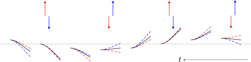
Figure 2: Kinematics of a heaving plate actuated at its first resonant frequency of $\sigma=3.1$. Shown are a plate with constant stiffness (solid black), time-periodic stiffness in phase with the motion ($\phi_{S}=0$; dashed blue), and time-periodic stiffness out of phase with the motion ($\phi_{S}=\pi$; dashed red). The colored arrows represent the difference between the instantaneous stiffness and the mean stiffness. The absence of arrows indicates the three plates have the same stiffness in the below snapshot. The parameters used are $\overline{S}=20$, $h_{0}=1$, $R=0.01$, and $|S_{0}|=0.5$.

First, we familiarize ourselves with how time-varying flexibility impacts the plate’s kinematics. Figure 2 shows the kinematics of three plates during one cycle of motion. The plates are all actuated at the same frequency—the first resonant frequency of the plate with constant stiffness, $\sigma=3.1$. The reference case with constant stiffness is compared against a plate with time-varying flexibility that is in phase with the motion ($\phi_{S}=0$), meaning it is stiff at the turn-around and flexible at mid-stroke, and a plate with time-varying flexibility that is out of phase with the motion ($\phi_{S}=\pi$), meaning it is flexible at the turn-around and stiff at the mid-stroke. For a plate with constant stiffness, the peak deflection occurs around the mid-stroke, where the lateral velocity is highest. For the $\phi_{S}=0$ case, the pressure on the plate is reduced throughout the mid-stroke with more deflection, and the increase in stiffness towards the turnaround causes it to catch back up to the reference case. Conversely, the $\phi_{S}=\pi$ case has its stiffness reduced at the turnaround, ultimately achieving the largest trailing edge deflection of all heave cases, and then recovering throughout the mid-stroke with increased stiffness. The stiffness oscillation essentially adds a phase lag relative to the motion of the constant-stiffness plate. When $\phi_{S}=\pi$, the motion leads that of the constant-stiffness plate, whereas when $\phi_{S}=0$, the motion lags that of the constant-stiffness plate.

In figure 3, we show how time-varying stiffness affects average thrust and efficiency. The frequency range is centered about the first resonant frequency of the plate with constant stiffness. Generally, adding periodic stiffness leads to a continuous and substantial increase in thrust as the stiffness oscillation amplitude increases, with up to a 35% increase in thrust when $|S_{0}|=0.5$. For $\phi_{S}=0$, the resonance is shifted to higher frequencies, while for $\phi_{S}=\pi$ the resonance is shifted lower compared to the constant stiffness case. Past the resonant frequency, the $\phi_{S}=\pi$ case yields slightly lower thrusts than the baseline case.

For efficiency, we observe the opposite behavior (figure 3b). Performance benefits for ${\phi_{S}=0}$ occur below the baseline resonant frequency, while for $\phi_{S}=\pi$ they occur above the baseline resonant frequency. For both phases of the stiffness oscillation, there are frequencies yielding greater efficiency than the constant-stiffness plate, as well as frequencies yielding lower efficiency. The effect of time-varying stiffness on the efficiency is much more mild than it is for thrust, however, as time-varying stiffness only changes the efficiency by $\Delta\eta\leq 0.05$. This suggests that time-varying stiffness may be a strategy to substantially increase thrust without much, if any, penalty in efficiency.

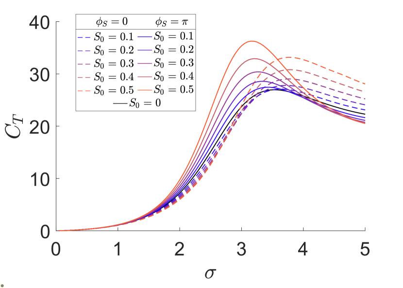
((a))

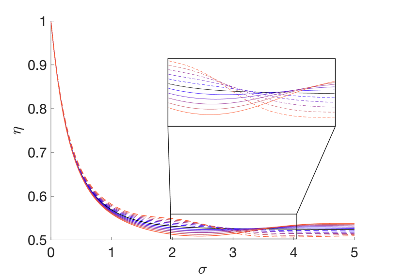
((b))

Figure 3: Thrust (left) and efficiency (right) for a heaving plate with gradually increasing stiffness oscillation amplitude. The parameters used are $\overline{S}=20$, $h_{0}=1$, and $R=0.01$.

To better understand the effects of time-varying stiffness, we turn to the time histories of the performance characteristics over the course of an actuation cycle. Figure 4 shows the instantaneous thrust, side force, and power coefficients over one period of the motion. For reference, we also plot the leading edge kinematics and plate stiffness. The plate with constant stiffness exhibits purely sinusoidal thrust, power, and side force since frequencies are uncoupled in the small-amplitude limit. Time-periodic stiffness, however, causes cross-frequency coupling, leading to non-sinusoidal behavior. Note that, because the stiffness oscillates at twice the frequency of motion, the side force remains symmetric, ensuring there is no mean side force (in a real system, this would lead to maneuvering).

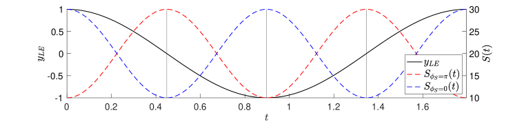
((a)) Kinematic input at the leading edge (solid black, left ordinate), and the stiffness distribution (blue and red dashed, right ordinate) for one stroke.

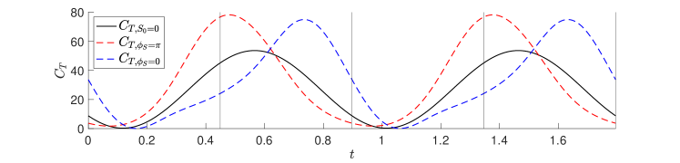
((b)) Thrust coefficient as a function of time.

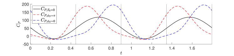
((c)) Power coefficient as a function of time.

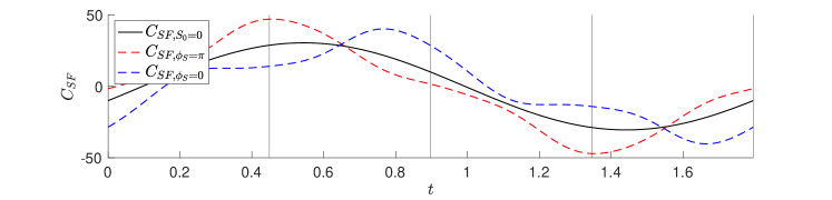
((d)) Side force coefficient as a function of time.

Figure 4: Instantaneous thrust, power, and side force coefficients for a heaving plate. The parameters used are $\overline{S}=20$, $h_{0}=1$, $R=0.01$, $\sigma=3.1$, and $|S_{0}|=0.5$. Shown are a plate with constant stiffness (solid black), time-periodic stiffness in phase with the motion ($\phi_{S}=0$; dashed blue), and time-periodic stiffness out of phase with the motion ($\phi_{S}=\pi$; dashed red).

The plate whose stiffness4 oscillates out of phase with the kinematics ($\phi_{S}=\pi$) produces the most thrust at the mid-stroke. During the turnaround the plate becomes the most flexible—this helps to relieve the power consumption which trends highest before the plate reverses direction. The opposite happens for the plate whose stiffness is in phase with the kinematics ($\phi_{S}=0$). It produces the most thrust closer to the turnaround, and the power relief comes when the plate is most flexible at the maximum plunge velocity. For both cases, higher thrust trends towards the times of higher stiffness, and lower power consumption trends towards the times of lower stiffness. The phase of the stiffness oscillation dictates when in the cycle the plate is most stiff (promoting thrust) or most flexible (relieving power). Thus, by timing these stiffness changes at opportune times during the cycle (e.g., becoming flexible at a time when power is highest), the performance can be significantly enhanced.

It is clear that the timing of the stiffness oscillation is important. However, until this point, only two stiffness oscillation phases have been considered: in phase and out of phase with the kinematics. We investigate whether there is a particular phase that maximizes thrust or efficiency. In figure 5, thrust and efficiency are plotted on a polar plot with frequency $\sigma$ on the radial axis and stiffness phase offset $\phi_{s}$ on the azimuthal axis. Both thrust and efficiency are shown relative to the constant-stiffness case. Time-varying stiffness increases thrust the most when $\phi_{S}$ is between $\pi/2$ and $2\pi/3$, and it increases efficiency the most near $\phi_{s}=3\pi/2$. Again, the changes in efficiency are modest. It is important here to also highlight the importance of the kinematic frequency—for a given phase of the stiffness oscillation, there can be performance boosts and hindrances depending on the frequency of oscillation.

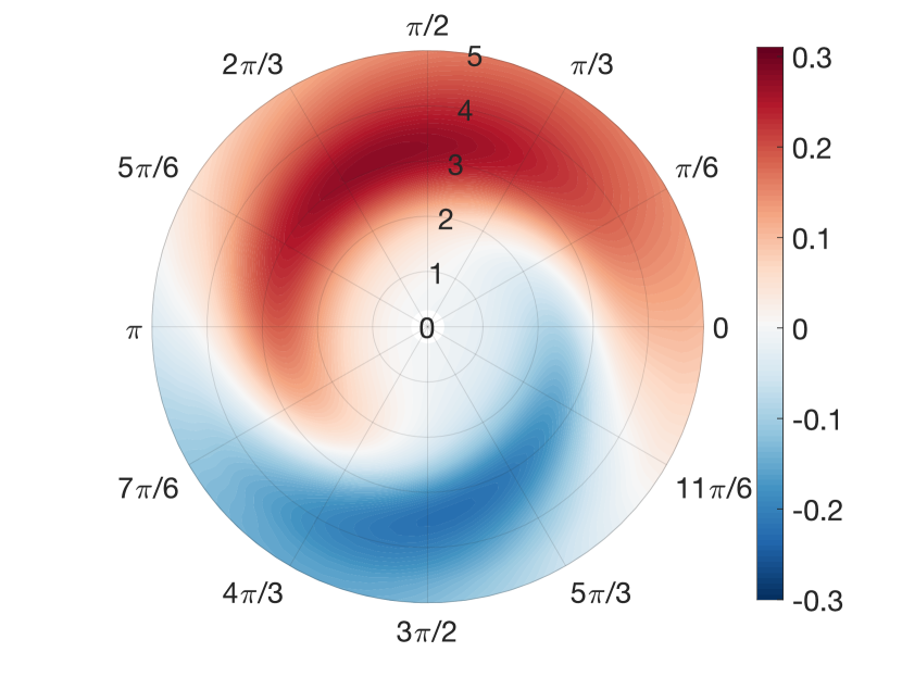
((a)) $\log{C_{T}/C_{T_{S_{0}=0}}}$

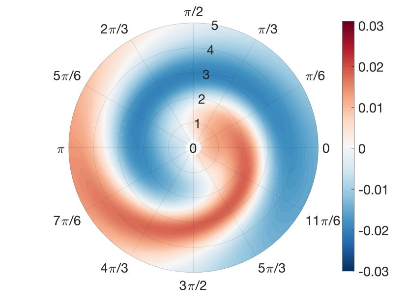
((b)) $\Delta\eta$

Figure 5: Impact of stiffness phase offset ($\phi_{S}$; azimuthal axis) and kinematic frequency ($\sigma$; radial axis) on thrust and efficiency for a heaving plate, relative to the constant-stiffness case. The parameters used are $\overline{S}=20$, $h_{0}=1$, $R=0.01$, and $|S_{0}|=0.5$.

We now explore a much wider range of mean plate stiffnesses and frequencies encompassing higher-order resonant frequencies. The change in swimming performance due to time-periodic stiffness, with respect to the constant-stiffness case, is shown in figure 6 for $\phi_{S}=0$ and $\pi$. The oscillation in stiffness modifies the resonant frequencies from those of the constant-stiffness plate, as we saw in figure 3, leading to sharp bands of increased and decreased thrust; these appear as adjacent narrow red and blue strips in figure 6. In a linear time-invariant system, resonant frequencies are related to the imaginary parts of the eigenvalues of the system, whereas in linear time-periodic systems, they are related to the imaginary parts of the Floquet exponents (Wereley, 1990). In general, the two are different, leading to the modified resonant frequencies that we observe. Away from resonance, thrust is modified little by the oscillation in stiffness. The changes in efficiency are much broader over the stiffness-frequency plane and have features that align with resonant frequencies; they are, however, very mild. Generally, thrust increases where efficiency decreases, but increasing $|S_{0}|$ can greatly increase the thrust production with minimal impact on efficiency. Note that we are using the small amplitude deflection and slope assumption while exploring resonance up to the second mode. One might assume that our assumption is invalid, due to the high deflections and slopes at the second resonance or higher. On the other hand, the kinematics of the plate scale linearly with the leading edge input. Therefore if we notice a deflection that would violate our assumption, we can just scale down our inputs until the deflection and slope satisfies the linear theory again.

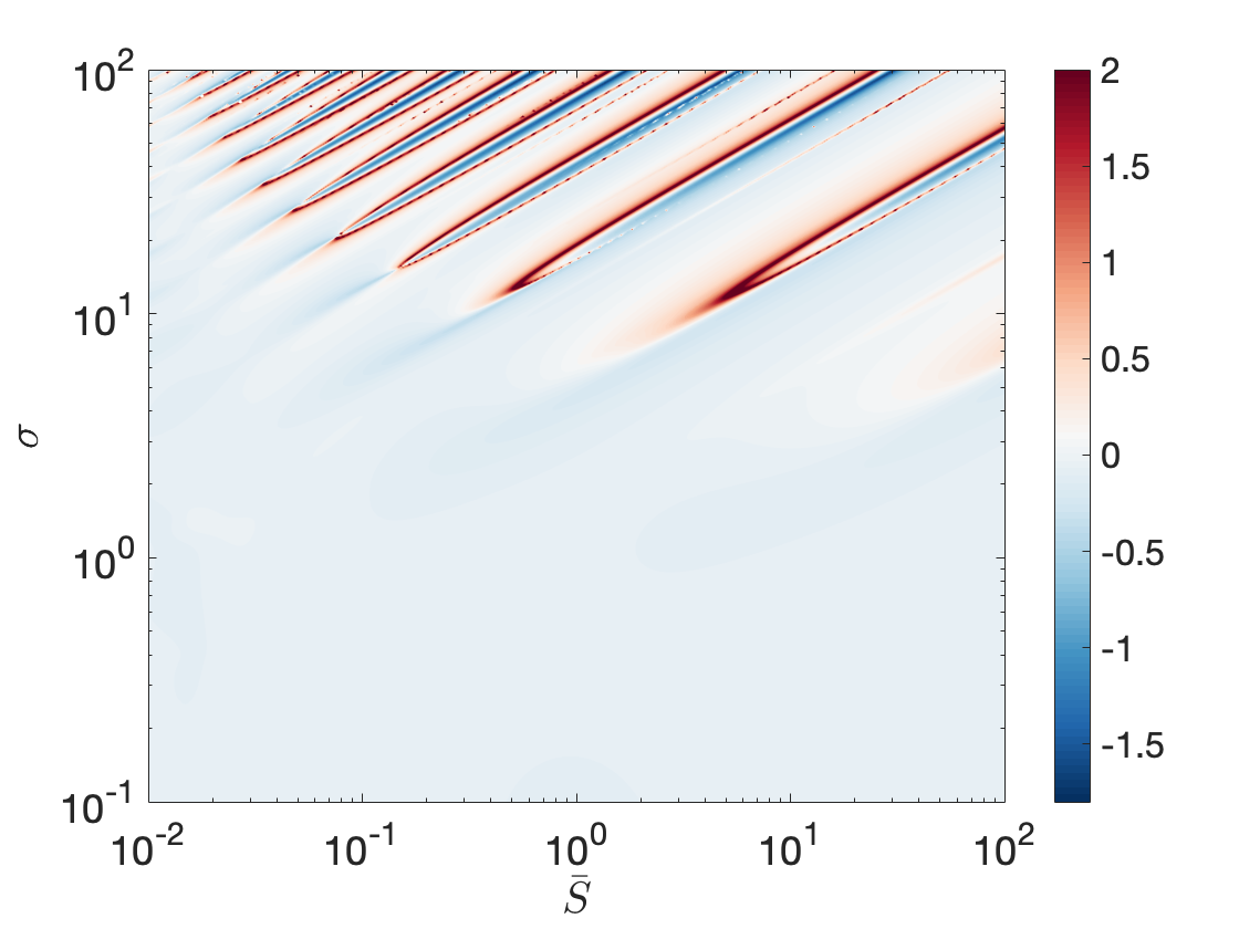
((a)) $\log{C_{T}/C_{T_{S_{0}=0}}}$
$\phi_{S}=0$

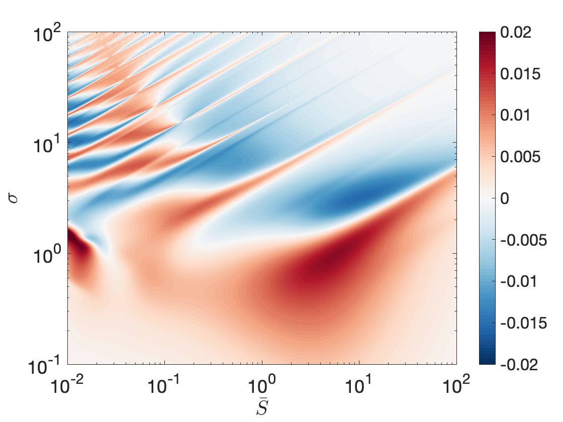
((b)) $\Delta\eta$
$\phi_{S}=0$

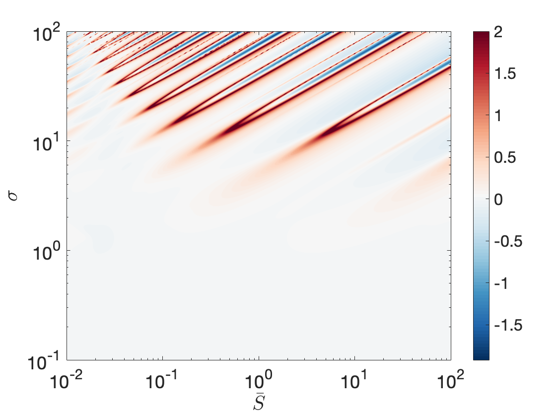
((c)) $\log{C_{T}/C_{T_{S_{0}=0}}}$
$\phi_{S}=\pi$

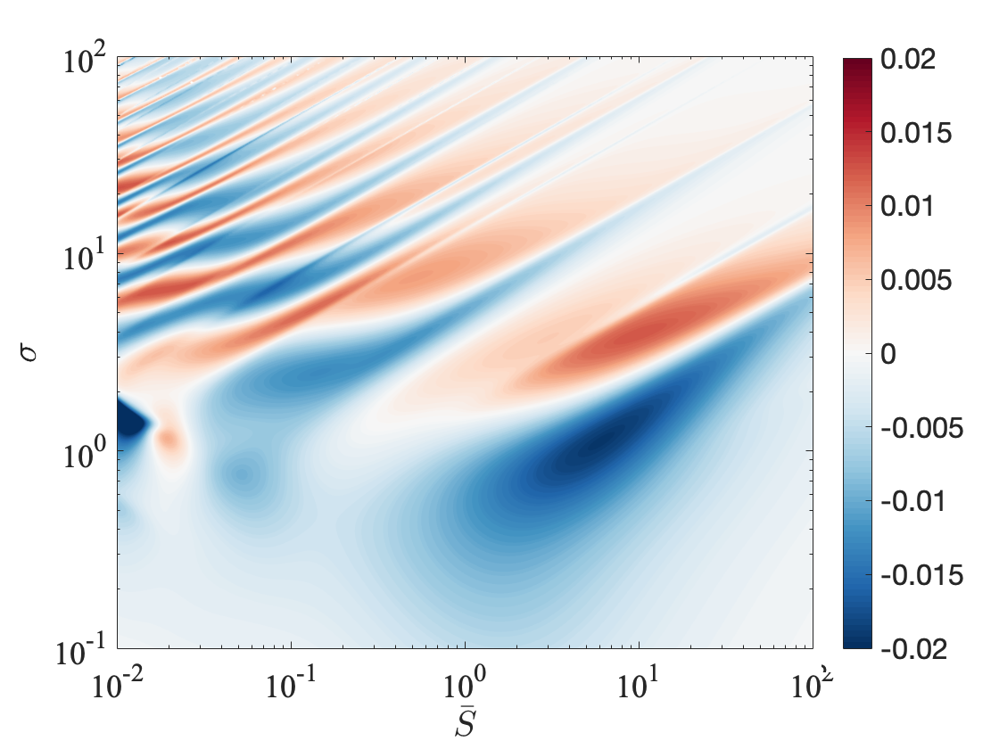
((d)) $\Delta\eta$
$\phi_{S}=\pi$

Figure 6: Impact of time-varying stiffness on the thrust (left) and efficiency (right), relative to the constant-stiffness case, for stiffness oscillations that are in phase with the motion (top), and 180^∘ out of phase with the motion (bottom). The parameters used are $h_{0}=1$, $R=0.01$, and $|S_{0}|=0.5$.

Perhaps the most interesting features in figure 6 are the hollowed peaks in the thrust, resembling the eye of a needle. They are more prominent at higher frequencies. To clarify this behavior, in figure 7 we show the thrust and efficiency along a slice in the stiffness-frequency plane, taking $\overline{S}=20$ and centering the frequency range about the second resonant frequency (this is the same parameter case as shown in figure 3). As the stiffness oscillation amplitude is gradually increased, there is a critical value of $|S_{0}|$ at which a single resonant peak in thrust bifurcates into two sharp peaks centered about the baseline resonant frequency, with the distance between the peaks increasing as $|S_{0}|$ increases. The bifurcated peaks are very sharp, indicative of natural frequencies with very little damping. Low damping leads to more energy input through the time-periodic stiffness then is dissipated through the wake and material damping, which leads to a net energy increase of the system ($\frac{dE}{dt}>0,\forall t>0$). This causes small perturbations in the kinematics to grow unbounded. To investigate this possibility, we perform a Floquet analysis.

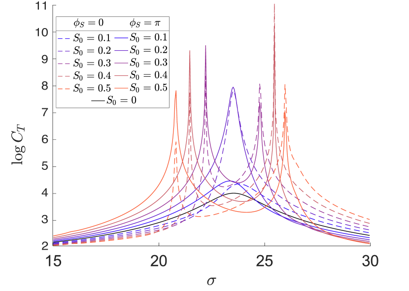
((a))

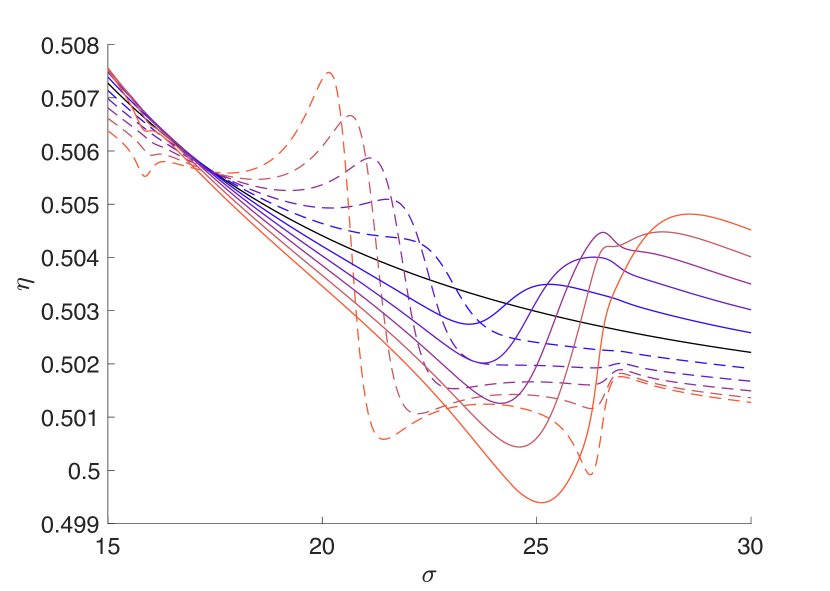
((b))

Figure 7: $\log C_{T}$ (left) and efficiency (right) for a heaving plate with gradually increasing stiffness oscillation amplitude. As stiffness oscillation amplitude $|S_{0}|$ increases, a single resonant peak bifurcates into two. The parameters used are $\overline{S}=20$, $h_{0}=1$, and $R=0.01$.

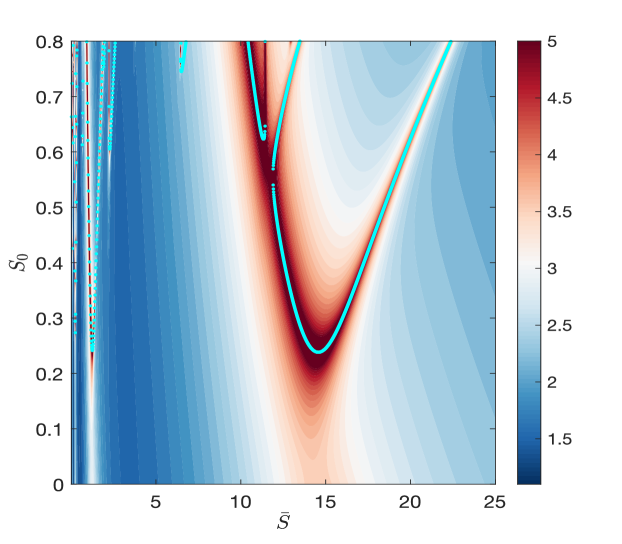
Figure 8: Neutral stability curves overlaid on contours of $\log C_{T}$. The parameters used are $R=0.01$ to calculate the neutral stability curves, and $h_{0}=1,\sigma=20,$ and $\phi_{S}=0$ to calculate the thrust values.

Representative results from the Floquet analysis are shown in figure 8. There, we have plotted the neutral curves in the $\overline{S}$-$|S_{0}|$ plane on top of contours of $\log C_{T}$. When the stiffness oscillation amplitude $|S_{0}|$ is below the neutral curves, the system is stable. Conversely, the system is unstable when $|S_{0}|$ is above the neutral curves. We see the emergence of tongues of instability, which are characteristic features of parametrically excited systems such as Mathieu’s equation (Nayfeh & Mook, 1995) and Faraday waves (Faraday, 1831; Miles & Henderson, 1990). Because the system is damped (due to energy lost to the wake via a thin sheet of vorticity), the instability emerges at a non-zero value of $|S_{0}|$. For a fixed value of $|S_{0}|$, as we vary the mean stiffness $\overline{S}$, we cross into and then out of the unstable region. At the boundaries, the thrust exhibits sharp peaks, which is explained by the theory of forced linear time-periodic systems (Wereley, 1990). This explains the double resonant peaks that we observed in figures 6 and 7. (Although we vary $\sigma$ at a fixed value of $\overline{S}$ in figure 7, we can see in figure 6 that we encounter double resonant peaks whether we vary $\overline{S}$ at a fixed value of $\sigma$, or we vary $\sigma$ at a fixed value of $\overline{S}$; physically, the origin of the double resonant peaks is the same.) No physical significance should be given to the thrust in the unstable region between the double resonant peaks since the thrust was calculated under the assumption of a stable system. We have verified for conditions other than those used to generate figure 8 that a splitting of one resonant peak into two coincides with the emergence of an instability; we conjecture that every region between double resonant peaks in figures 6 and 7 is actually unstable. While instability usually has a negative connotation in engineering applications, these unstable regions could potentially lead to greatly enhanced propulsive performance since an instability would produce large deflections from small actuation. Our linear method cannot capture the saturation of the instabilities, but we believe that exploring the unstable regions via experiments or nonlinear simulations is a promising direction. We believe that Shi et al. (2020) does not see these instabilities due to the use of the nonlinear beam equation, which would delay the emergence of the instabilities to higher resonant frequences.

3.2 Pitch-only and pitch-and-heave motions

We now consider how pitching the leading edge changes the results. As stated previously, pitching and heaving are fundamentally different in their thrust generation mechanism (Floryan et al., 2017a; Van Buren et al., 2020), with the former utilizing added-mass forces and the latter using lift-based or circulatory forces. Additionally, combined pitching and heaving motions are the most biologically relevant and also the best-performing (Van Buren et al., 2019; Wu, 2011). In this section, we study two cases: (1) purely pitching, and (2) combined pitching and heaving with pitch lagging heave by $\pi/2$, the most ‘fish-like’ motion that is also generally the most efficient (Van Buren et al., 2019; Triantafyllou et al., 2000).

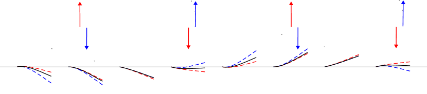
((a))

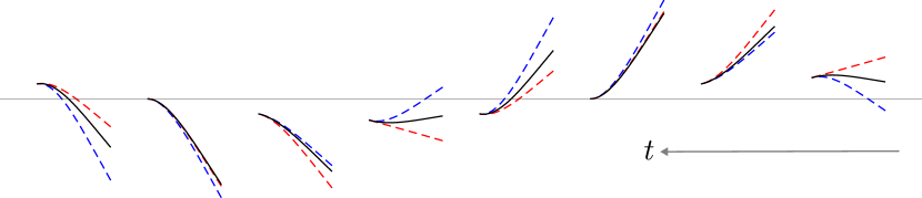
((b))

Figure 9: Analogous to figure 2, but for a pitching plate (top) and a pitching and heaving plate (bottom). Shown are a plate with constant stiffness (solid black), time-periodic stiffness in phase with the motion ($\phi_{S}=0$; dashed blue), and time-periodic stiffness out of phase with the motion ($\phi_{S}=\pi$; dashed red). The parameters used are $\overline{S}=20$, $h_{0}=1$, $\theta_{0}=-0.5j$, $R=0.01$, and $|S_{0}|=0.5$.

Figure 9 shows the kinematics for both cases during one cycle of motion. The kinematics are qualitatively the same as for the purely heaving case in figure 2. Adding an oscillatory component to the stiffness causes a lead/lag effect on the kinematics which dictates at what point in the stroke thrust is generated. When the stiffness is in phase with the motion, rapid trailing edge motion occurs near the turnaround where the plate transitions from flexible to stiff, whereas when the stiffness is out of phase with the motion, the rapid trailing edge motion occurs through the midpoint of the cycle. Even for the pitching and heaving case—which specifically reduces the side-force on the plate (Van Buren et al., 2019)—we see the stiffness oscillations have similar impact in both magnitude and timing.

Figure 10 shows the thrust and efficiency for the two cases in a frequency range centered about the first resonant frequency of the plate with constant stiffness. For both the pitch and pitch-and-heave cases, we see that the oscillating stiffness has a strong impact on the peak thrust near resonance. The efficiency is less impacted by the stiffness oscillation and switches from being greater than the efficiency of a constant-stiffness plate to less than it across the resonant frequency—depending on the phase of the stiffness oscillation—which is similar to the behavior of the purely heaving plate in figure 3. For the purely pitching plate, thrust is much more impacted by the oscillating stiffness when it is out of phase with the kinematics, $\phi_{S}=0$. For pitching, the blue plate lags behind the red and black plate at the turnaround, and becomes the least stiff at this moment. The blue plate accelerates the fastest between frames 2 and 4 in figure 9, which corresponds to the fastest angular velocity at the leading edge. The blue plate had the highest trailing edge amplitude, because the phase difference between the leading edge input and the trailing edge deflection and its lower stiffness allows the blue plate to reach a higher trailing edge amplitude before feeling the effects of the acceleration at the leading edge. The blue plate then becomes stiffer as the effect of the acceleration at the leading edge reaches the trailing edge. This combination of high acceleration, high trailing edge amplitude, and high stiffness creates high thrust. The red plate’s stiffness distribution is misaligned with the phase difference caused by pure pitching, and therefore reaches a lower max trailing edge amplitude, and benefit less from the high acceleration of the leading edge between frames 2 and 4 in figure 9. For a better visualization of the plate dynamics and how they tie into the performance enhancements, refer to the online supplemental movies where we show the heave, pitch, and heave plus pitch kinematics.

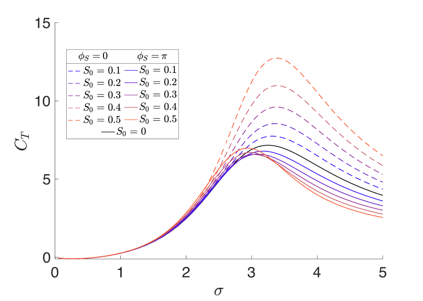
((a)) $C_{T}$
$h=0,\theta=0.5$

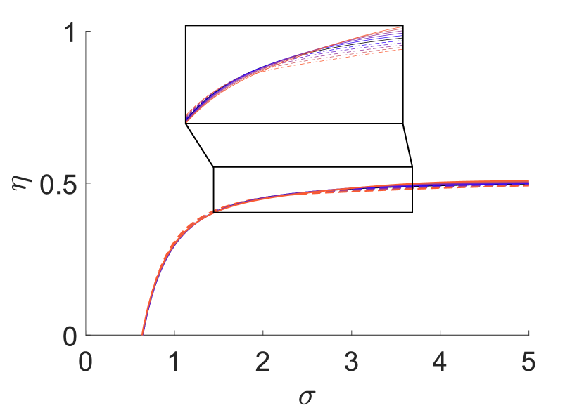
((b)) $\Delta\eta$
$h=0,\theta=0.5$

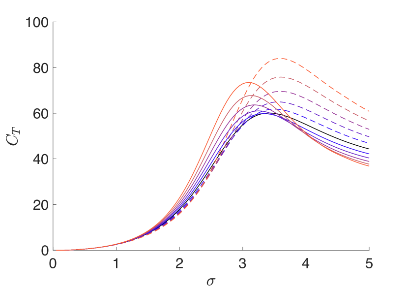
((c)) $C_{T}$
$h=1,\theta=0.5$

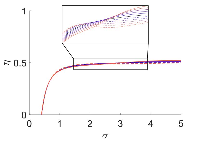
((d)) $\Delta\eta$
$h=1,\theta=0.5$

Figure 10: Thrust and efficiency of a purely pitching plate (top) and a pitching and heaving plate (bottom) as a function of driving frequency $\sigma$. The parameters used are $\overline{S}=20$, $h_{0}=1$, $\theta_{0}=-0.5j$, and $R=0.01$.

Finally, we consider the role of the phase of stiffness oscillation in more detail. Figure 11 shows the change in thrust and efficiency relative to the constant-stiffness case. For the heaving plate, the ideal phase for thrust was approximately between $\pi/2$ and $2\pi/3$; for the pitching plate, however, the ideal phase is approximately $\pi/3$. The ideal phase for the combined pitching and heaving plate is approximately $\pi/2$, directly between the isolated pitching and heaving cases. Generally, the efficiency has opposing behavior to the thrust, with increased thrust coinciding with decreased propulsive efficiency.

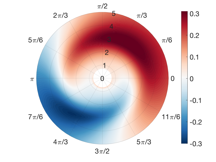
((a)) $\log{C_{T}/C_{T_{S_{0}=0}}}$
$h=0,\theta=0.5$

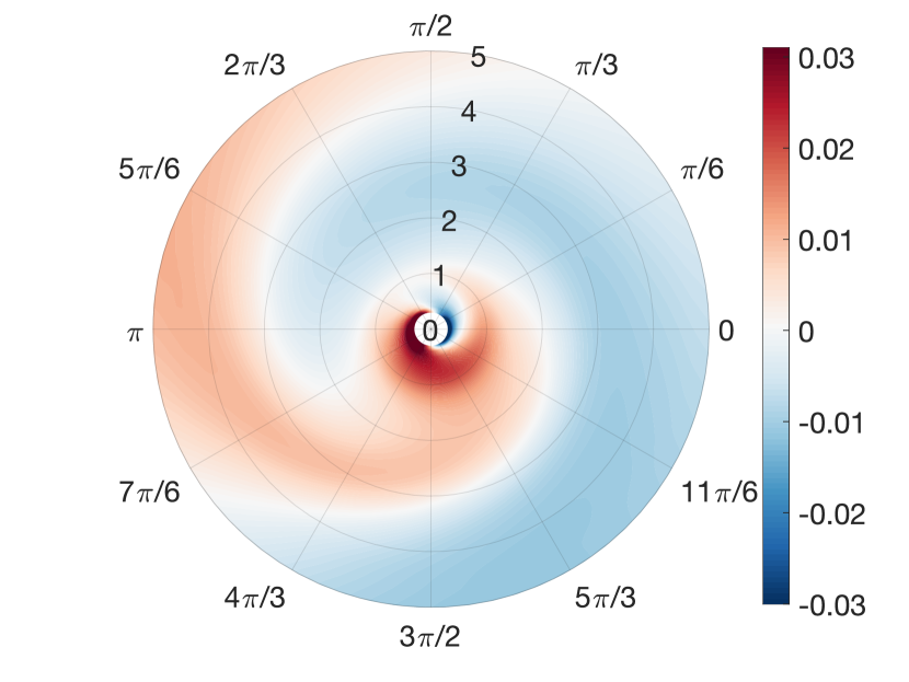
((b)) $\Delta\eta$
$h=0,\theta=0.5$

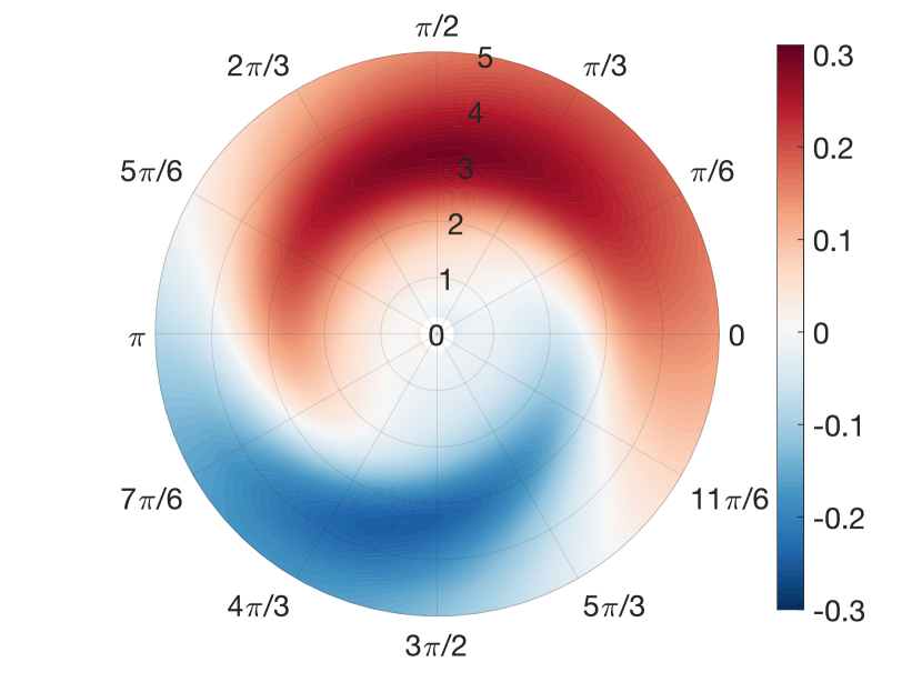
((c)) $\log{C_{T}/C_{T_{S_{0}=0}}}$
$h=1,\theta=0.5$

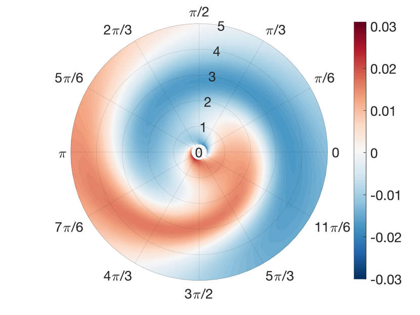
((d)) $\Delta\eta$
$h=1,\theta=0.5$

Figure 11: Impact of stiffness phase offset ($\phi_{S}$; azimuthal axis) and kinematic frequency ($\sigma$; radial axis) on thrust and efficiency for a pitching (top) and a pitching and heaving (bottom) plate, relative to the constant-stiffness case. Note the white unit circles on the efficiency contours. They are whited out due to large negative efficiency values, which detract from the regions of interest. The parameters used are $\overline{S}=20$, $h_{0}=1$, $\theta_{0}=-0.5j$, $R=0.01$, and $|S_{0}|=0.5$.

4 Conclusions

In this work, we explore the impact of time-periodic stiffness on an oscillating plate in a free stream—a model for swimmers. The stiffness oscillations were varied in amplitude and phase and consistently compared to the baseline constant-stiffness case. The stiffness oscillation frequency is fixed at twice the kinematic frequency to enforce zero mean side force, which is required for rectilinear swimming. The fluid-structure interaction model is solved using a spectral method first introduced in Moore (2017), modified to account for time-periodic stiffness.

It is shown that the oscillation in stiffness has a significant impact on the thrust and kinematics. The impact on thrust is most prominent, with time-periodic stiffness increasing thrust by up to 35% at the first resonant peak. The impact on efficiency is, on the other hand, mild, with the efficiency changing by $\Delta\eta\leq 0.05$. These results align well with Shi et al. (2020). The changes in thrust and efficiency are often negatively correlated. These performance changes are consistent across heaving, pitching, and combined pitch-and-heave motions.

The performance alteration due to time-varying stiffness is strongly linked to the phase of the stiffness oscillation. This is because thrust and side forces are produced at different stages throughout the kinematic cycle, and whether the plate is more or less stiff at those stages either yields enhanced thrust or power reduction. This is especially evident when comparing pure heaving motions to pure pitching motions, which have different phase differences between the leading edge input and the trailing edge deflection.

When the kinematic frequency and amplitude of stiffness oscillation are large enough, instabilities emerge in regions of parameter space centered about resonant frequencies of the constant-stiffness plate. Our linear method cannot capture the saturation of the instabilities, but we anticipate that the unstable regions of parameter space may yield enhanced propulsive performance. Exploring the unstable regions via experiments or nonlinear simulations is a promising future research direction.

While there may not yet be concrete evidence of biological swimmers actively changing their stiffness on the time scale of their kinematic frequency, we have presented strong evidence that there would be a hydrodynamic benefit to doing so. This may be a promising avenue to pursue when designing robotic swimmers.

Appendix A Method of solution

We assume the kinematics $Y$, the hydrodynamic load $q=\Delta p$, and the stiffness ratio $S$ are periodic in time and can be expressed as Fourier series,

$$Y(x,t) =\sum_{m=-\infty}^{\infty}\hat{y}_{m}(x)e^{jm\sigma t},$$ (12a)

$$q(x,t) =\sum_{m=-\infty}^{\infty}\hat{q}_{m}(x)e^{jm\sigma t},$$ (12b)

$$S(t) =\sum_{m=-\infty}^{\infty}\hat{S}_{m}e^{jm\sigma t}.$$ (12c)

Substituting these expressions into (3) gives

$$\sum_{m=-\infty}^{\infty}\hat{q}_{m}(x)e^{jm\sigma t}+2R\sum_{m=-\infty}^{\infty}m^{2}\sigma^{2}\hat{y}_{m}(x)e^{jm\sigma t}-\frac{2}{3}\sum_{m=-\infty}^{\infty}\sum_{k=-\infty}^{\infty}\hat{S}_{m-k}\hat{y}_{k}^{\prime\prime\prime\prime}(x)e^{jm\sigma t}=0,$$ (13)

where a prime denotes differentiation with respect to $x$. Separating the Fourier components yields the following system of ordinary differential equations,

$$\hat{q}_{m}(x)+2m^{2}\sigma^{2}R\hat{y}_{m}(x)-\frac{2}{3}\sum_{k=-\infty}^{\infty}\hat{S}_{m-k}\hat{y}^{\prime\prime\prime\prime}_{k}(x)=0,\quad\forall m\in\mathbb{Z}.$$ (14)

Expanding the heaving and pitching motions into Fourier series as

$$h(t)=\sum_{m=-\infty}^{\infty}\hat{h}_{m}e^{jm\sigma t},$$ (15a)

$$\theta(t)=\sum_{m=-\infty}^{\infty}\hat{\theta}_{m}e^{jm\sigma t},$$ (15b)

and substituting them and (12a) into (7) gives boundary conditions for the $\hat{y}_{m}$:

$$\hat{y}_{m}(-1)=\hat{h}_{m},\;\;\;\hat{y}^{\prime}_{m}(-1)=\hat{\theta}_{m},\;\;\;\hat{y}^{\prime\prime}_{m}(1)=\hat{y}^{\prime\prime\prime}_{m}(1)=0,\quad\forall m\in\mathbb{Z}.$$ (16)

We also require that all the functions are real, leading to the reality conditions,

$$\hat{y}_{m}(x)=\hat{y}_{-m}^{*}(x),\;\hat{q}_{m}(x)=\hat{q}_{-m}^{*}(x),\;\hat{S}_{m}=\hat{S}_{-m}^{*},\;\hat{h}_{m}=\hat{h}_{-m}^{*},\;\hat{\theta}_{m}=\hat{\theta}_{-m}^{*},\quad\forall m\in\mathbb{Z},$$ (17)

where the superscript $*$ again denotes complex conjugation.

Given the hydrodynamic load $q$, the stiffness ratio $S$, and the heaving and pitching actuation at the leading edge, we can solve for the kinematics $Y$ by solving the system of coupled ordinary differential equations given by (14) along with their boundary conditions given by (16). What remains is to couple the solid and fluid mechanics by expressing the hydrodynamic load in terms of the kinematics, which we do next.

The pressure difference across the plate creates the hydrodynamic load, and is related to Prandtl’s acceleration potential by

$$\Delta p=\phi_{\text{top}}-\phi_{\text{bottom}}.$$

Taking the divergence of (4b) and using incompressibility shows that $\phi$ is harmonic, implying the existence of a harmonic conjugate $\psi$. We define the complex acceleration potential

$$F(x,y,t)=\phi(x,y,t)+i\psi(x,y,t),$$ (18)

where $i=\sqrt{-1}$. It will be convenient to work with the complex variable $z=x+iy$. Note that $F$ is analytic in $z$. We conformally map the physical $z$ plane to the exterior of the unit disk in the $\zeta$ plane using

$$z=\frac{1}{2}\left(\zeta+\frac{1}{\zeta}\right).$$ (19)

Because the acceleration potential $F$ is conformally invariant under 19, $F$ is analytic in $\zeta$ and can be represented by a multipole expansion,

$$F=i\left(\frac{a_{0}(t)}{\zeta+1}+\sum_{k=1}^{\infty}\frac{a_{k}(t)}{\zeta^{k}}\right),$$ (20)

where the coefficients $a_{k}$ are real (Wu, 1961). The first term represents the singularity at the leading edge, and the infinite series represents an analytic function that is regular on and outside the unit circle, decaying in the far field (Wu, 1961).

Continuing with our assumption of a time-periodic flow, we expand the coefficients in the multipole expansion into Fourier series,

$$a_{k}(t)=\sum_{m=-\infty}^{\infty}\hat{a}_{k,m}e^{jm\sigma t},\quad\forall k\in\mathbb{W}.$$ (21)

Substituting (21) into (20) yields

$$F=i\left(\frac{1}{\zeta+1}\sum_{m=-\infty}^{\infty}\hat{a}_{0,m}e^{jm\sigma t}+\sum_{k=1}^{\infty}\frac{1}{\zeta^{k}}\sum_{m=-\infty}^{\infty}\hat{a}_{k,m}e^{jm\sigma t}\right),$$ (22)

which we can rewrite as a Fourier expansion of $F$,

$$F=\sum_{m=-\infty}^{\infty}\hat{F}_{m}e^{jm\sigma t}=\sum_{m=-\infty}^{\infty}i\left(\frac{\hat{a}_{0,m}}{\zeta+1}+\sum_{k=1}^{\infty}\frac{\hat{a}_{k,m}}{\zeta^{k}}\right)e^{jm\sigma t}.$$ (23)

Evaluating (23) on the unit circle ($\zeta=e^{i\theta}$), which corresponds to the surface of the plate in the $z$ plane, and separating the real and imaginary parts yields

$$\phi|_{W} =\sum_{m=-\infty}^{\infty}\left(\frac{1}{2}\hat{a}_{0,m}\tan\frac{\theta}{2}+\sum_{k=1}^{\infty}\hat{a}_{k,m}\sin{k\theta}\right)e^{jm\sigma t},$$ (24a)

$$\psi|_{W} =\sum_{m=-\infty}^{\infty}\left(\frac{1}{2}\hat{a}_{0,m}+\sum_{k=1}^{\infty}\hat{a}_{k,m}\cos{k\theta}\right)e^{jm\sigma t}=\sum_{m=-\infty}^{\infty}\Psi_{m}(x)e^{jm\sigma t}.$$ (24b)

We recognize the expression for $\Psi_{m}(x)$ as a Chebyshev series in $x$,

$$\Psi_{m}(x)=\frac{1}{2}\hat{a}_{0,m}+\sum_{k=1}^{\infty}\hat{a}_{k,m}T_{k}(x),\quad\forall m\in\mathbb{Z},$$ (25)

where $T_{k}(x)=\cos(k\arccos x)$ is the $k$th Chebyshev polynomial, and $x=\cos\theta$.

The complex acceleration potential can be related to the complex velocity $w=u-iv$ through the momentum equation, (4b), by

$$\frac{\partial F}{\partial z}=\frac{\partial w}{\partial t}+\frac{\partial w}{\partial z}.$$ (26)

Evaluating the imaginary part on the plate’s surface ($z=x$) and substituting the no-penetration boundary condition, (6a), yields

$$\frac{\partial\psi}{\partial x}\Bigr{|}_{y=0}=-\left(\frac{\partial}{\partial t}+\frac{\partial}{\partial x}\right)^{2}Y.$$ (27)

Substituting (12a) and (24b) into (27) gives

$$\sum_{m=-\infty}^{\infty}\mathcal{D}\Psi_{m}(x)e^{jm\sigma t}=-\sum_{m=-\infty}^{\infty}(jm\sigma+\mathcal{D})^{2}\hat{y}_{m}(x)e^{jm\sigma t},$$ (28)

where $\mathcal{D}=\frac{\text{d}}{\text{d}x}$. Separating Fourier components gives

$$\mathcal{D}\Psi_{m}(x)=-(jm\sigma+\mathcal{D})^{2}\hat{y}_{m}(x),\quad\forall m\in\mathbb{Z}.$$ (29)

Given $\hat{y}_{m}$, we expand it into a Chebyshev series and use (29) to express the Chebyshev coefficients of $\Psi_{m}$—that is, $\hat{a}_{k,m}$ for $k\geq 1$—in terms of the Chebyshev coefficients of $\hat{y}_{m}$. To determine $\hat{a}_{0,m}$, we expand the vertical velocity on the plate in a Fourier series,

$$v|_{W}=\sum_{m=-\infty}^{\infty}\hat{v}_{m}(x)e^{jm\sigma t},$$ (30)

and the spatial coefficients in Chebyshev series,

$$\hat{v}_{m}(x)=\frac{1}{2}\hat{V}_{0,m}+\sum_{k=1}^{\infty}\hat{V}_{k,m}T_{k}(x),\quad\forall m\in\mathbb{Z}.$$ (31)

We can express the no-penetration boundary condition, (6a), as

$$\hat{v}_{m}(x)=(jm\sigma+\mathcal{D})\hat{y}_{m}(x),\quad\forall m\in\mathbb{Z}.$$ (32)

Given the Chebyshev coefficients of $\hat{y}_{m}$, (32) gives the Chebyshev coefficients of $\hat{v}_{m}$. The coefficient $\hat{a}_{0,m}$ is then given by

$$\hat{a}_{0,m}=-C(jm\sigma)(\hat{V}_{0,m}+\hat{V}_{1,m})+\hat{V}_{1,m},\quad\forall m\in\mathbb{Z},$$ (33)

where

$$C(jm\sigma)=\frac{K_{1}(jm\sigma)}{K_{0}(jm\sigma)+K_{1}(jm\sigma)}$$ (34)

is the Theodorsen function, and $K_{\nu}$ is the modified Bessel function of the second kind of order $\nu$. The expression for $\hat{a}_{0,m}$ is derived in Wu (1961).

With all the $\hat{a}_{k,m}$ in hand, the hydrodynamic load is given by

$$\hat{q}_{m}(x)=\hat{a}_{0,m}\sqrt{\frac{1-x}{1+x}}+2\sum_{k=1}^{\infty}\hat{a}_{k,m}\sin k\theta,\quad\forall m\in\mathbb{Z}.$$ (35)

The hydrodynamic load $\hat{q}_{m}$ depends linearly on $\hat{y}_{m}$.

To summarize, given the kinematics $\hat{y}_{m}$, we can calculate the coefficients $\hat{a}_{k,m}$, with which we can calculate the hydrodynamic load, which alters the kinematics via (14). The coupled fluid-structure problem must be solved numerically. The pseudospectral numerical method for constant stiffness is given by Moore (2017), which is relatively straightforward to adapt to account for time-periodic stiffness; in it, the kinematics are expanded into Chebyshev series. All infinite series are truncated to finite series; for the results presented in this work, we have used 16 Fourier modes and 64 Chebyshev modes. The method is fast and accurate, pre-conditioning the system with continuous operators to avoid errors typically encountered when using spectral methods to solve high-order differential equations. Formulas to calculate the thrust and power coefficients are given in Moore (2017).

Appendix B Floquet analysis

To test the stability of the solutions computed using the method in Appendix A, we perform a Floquet analysis of the problem with homogeneous boundary conditions. This analysis is adapted from the eigenvalue problem described by Floryan & Rowley (2018, 2020). Following the preceding analysis, but not assuming a form for the time dependence, we arrive at

$$2RY_{tt}+\frac{2}{3}S(t)Y_{xxxx}=\Delta p,$$ (36a)

$$Y(x,t)=\frac{1}{2}y_{0}(t)+\sum_{k=1}^{\infty}y_{k}(t)T_{k}(x),$$ (36b)

$$\Delta p(x,t)=a_{0}(t)\sqrt{\frac{1-x}{1+x}}+2\sum_{k=1}^{\infty}a_{k}(t)\sin{k\theta},$$ (36c)

$$\sum_{k=1}^{\infty}a_{k}(t)T_{k}^{\prime}(x)=-\frac{1}{2}\ddot{y}_{0}(t)-\sum_{k=1}^{\infty}[\ddot{y}_{k}(t)T_{k}(x)+2\dot{y}_{k}(x)T_{k}^{\prime}(x)+y_{k}(t)T_{k}^{\prime\prime}(x)],$$ (36d)

$$Y(-1,t)=0,\quad Y_{x}(-1,t)=0,\quad Y_{xx}(1,t)=Y_{xxx}(1,t)=0.$$ (36e)

Above, a dot denotes differentiation with respect to $t$. In (36b), we have written $Y$ as a Chebyshev series in $x$. The expression in (36d) derives from the no-penetration condition (27).

In what follows, we set $S(t)=\overline{S}+\frac{\overline{S}S_{0}}{2}(e^{j\omega t}+e^{-j\omega t})$, as in (11c). Here, $\omega$ is the frequency of the stiffness oscillation. Assuming the Floquet solution form,

$$y_{k}(t) =e^{\lambda t}\sum_{m=-\infty}^{\infty}\hat{y}_{k,m}e^{jm\omega t},$$ (37a)

$$a_{k}(t) =e^{\lambda t}\sum_{m=-\infty}^{\infty}\hat{a}_{k,m}e^{jm\omega t},\quad\forall k\in\mathbb{W},$$ (37b)

where $\lambda$ is the Floquet exponent, gives, after separating the Fourier components, the following set of equations,

$$2R(\lambda+jm\omega)^{2}\hat{\boldsymbol{y}}_{m}+\frac{2}{3}\overline{S}\mathbf{D}^{4}\hat{\boldsymbol{y}}_{m}+\frac{1}{3}\overline{S}S_{0}\mathbf{D}^{4}\hat{\boldsymbol{y}}_{m-1}+\frac{1}{3}\overline{S}S_{0}\mathbf{D}^{4}\hat{\boldsymbol{y}}_{m+1}=\hat{\boldsymbol{p}}_{m},$$ (38a)

$$\hat{\boldsymbol{p}}_{m}=\mathbf{A}\hat{\boldsymbol{a}}_{m},$$ (38b)

$$\mathbf{D}\hat{\boldsymbol{a}}_{m}=-(\lambda+jm\omega)^{2}\hat{\boldsymbol{y}}_{m}-2(\lambda+jm\omega)\mathbf{D}\hat{\boldsymbol{y}}_{m}-\mathbf{D}^{2}\hat{\boldsymbol{y}}_{m},$$ (38c)

$$\hat{\boldsymbol{V}}_{m}=(\lambda+jm\omega)\hat{\boldsymbol{y}}_{m}+\mathbf{D}\hat{\boldsymbol{y}}_{m},$$ (38d)

$$\hat{a}_{0,m}=-C(\lambda+jm\omega)(\hat{V}_{0,m}+\hat{V}_{1,m})+\hat{V}_{1,m},\quad\forall m\in\mathbb{Z}.$$ (38e)

Above, $\hat{\boldsymbol{y}}_{m}$ is a vector of the Chebyshev coefficients corresponding to index $m$ in (37a): $\hat{\boldsymbol{y}}_{m}=\begin{bmatrix}\hat{y}_{0,m}&\hat{y}_{1,m}&\hat{y}_{2,m}&\cdots\end{bmatrix}^{T}$; analogous expressions hold for $\hat{\boldsymbol{p}}_{m}$ (pressure), $\hat{\boldsymbol{a}}_{m}$ (potential), and $\hat{\boldsymbol{V}}_{m}$ (vertical velocity). The equality in (38b) states that the Chebyshev coefficients of the pressure are linear combinations of the Chebyshev coefficients of the potential, and $\mathbf{D}$ is the differentiation operator in Chebyshev space. Putting these equations together gives

$$\begin{split}\mathbf{A}[\mathbf{e_{1}}(\mathbf{e_{2}}-C(\lambda_{m})\mathbf{e_{1}}-C(\lambda_{m})\mathbf{e_{2}})^{T}(\lambda_{m}\boldsymbol{\hat{y}}_{m}+\mathbf{D}\boldsymbol{\hat{y}}_{m})-\lambda_{m}^{2}\mathbf{D^{-}}\boldsymbol{\hat{y}}_{m}-2\lambda_{m}\mathbf{D^{-}}\mathbf{D}\boldsymbol{\hat{y}}_{m}\\ -\mathbf{D^{-}}\mathbf{D^{2}}\boldsymbol{\hat{y}}_{m}]-2R\lambda_{m}^{2}\boldsymbol{\hat{y}}_{m}-\frac{2}{3}\mathbf{D^{4}}\overline{S}\boldsymbol{\hat{y}}_{m}=\frac{\overline{S}S_{0}}{3}\mathbf{D}^{4}[\boldsymbol{\hat{y}}_{m-1}+\boldsymbol{\hat{y}}_{m+1}],\quad\forall m\in\mathbb{Z},\end{split}$$ (39)

where $\lambda_{m}=\lambda+jm\omega$, $\mathbf{D^{-}}$ is the Chebyshev-space representation of the integration operator that makes the first Chebyshev coefficient zero, and $\mathbf{e}_{k}$ is the $k$th Euclidean basis vector.

Because of the presence of the Theodorsen function, solving for the Floquet exponents requires solving a nonlinear generalized eigenvalue problem. Since we are mainly interested in delineating regions of parameter space where solutions are unstable, we instead follow the idea of Kumar & Tuckerman (1994) to find the marginal stability curves. Rather than calculating the Floquet exponents for given values of the parameters, we set the value of the Floquet exponent such that $Re(\lambda)=0$ and solve for $S_{0}$. Physically, we are trying to find the strength of the stiffness oscillation that borders regions of stability and instability. This leads to a linear generalized eigenvalue problem where $S_{0}$ is the eigenvalue. Note that we must also set a value for $Im(\lambda)\in[0,\omega]$; $Im(\lambda)=0$ is called the harmonic case, and $Im(\lambda)=\omega/2$ is called the subharmonic case (Kumar & Tuckerman, 1994).

As can be seen in (39), the time dependence of the stiffness causes cross-frequency coupling in the kinematics. We write (39) compactly as

$$\mathbf{B}_{m}\boldsymbol{\hat{y}}_{m}=\frac{\overline{S}S_{0}}{3}\mathbf{C}_{m}\boldsymbol{\hat{y}}_{m},\quad\forall m\in\mathbb{Z},$$ (40)

where,

$$\mathbf{B}_{m}= \mathbf{A}[\mathbf{e_{1}}(\mathbf{e_{2}}-C(\lambda_{m})\mathbf{e_{1}}-C(\lambda_{m})\mathbf{e_{2}})^{T}(\lambda_{m}\mathbf{I}+\mathbf{D})-\lambda_{m}^{2}\mathbf{D^{-}}-2\lambda_{m}\mathbf{D^{-}}\mathbf{D}-\mathbf{D^{-}}\mathbf{D^{2}}]$$

$$-2R\lambda_{m}^{2}\mathbf{I}-\frac{2}{3}\boldsymbol{D^{4}}\overline{S},\quad\forall m\in\mathbb{Z}.$$

The operator $\mathbf{C}_{m}$ maps $\boldsymbol{\hat{y}}_{m}$ to $\mathbf{D}^{4}(\boldsymbol{\hat{y}}_{m+1}+\boldsymbol{\hat{y}}_{m-1})$. This is a linear generalized eigenvalue problem where the eigenvalues are the amplitudes of the stiffness oscillation, $S_{0}$.

To proceed, we truncate all Chebyshev expansions to the upper limit $N$, and truncate all Fourier expansions so that they contain frequencies up to $M\omega$. Doing so makes $\boldsymbol{\hat{y}}_{m}$ a vector of length $N+1$. We must simultaneously solve the system (40) for all $\boldsymbol{\hat{y}}_{m}$, leading to a system of size $2M(N+1)\times 2M(N+1)$. We choose $N=16$ and $M=11$. We reduce the order of the Chebyshev and Fourier modes so the Floquet problem can be solved in reasonable time.

In the harmonic ($Im(\lambda)=0$) and subharmonic ($Im(\lambda)=\omega$) cases, $\boldsymbol{\hat{y}}_{m}$ must obey the reality conditions: $\boldsymbol{\hat{y}}_{-m}=\boldsymbol{\hat{y}}_{m}^{*}$ in the harmonic case, and $\boldsymbol{\hat{y}}_{-m}=\boldsymbol{\hat{y}}_{m-1}^{*}$ in the subharmonic case. The reality conditions allow us to rewrite the Fourier expansions in terms of only non-negative indices. For $0<Im(\lambda)<\omega$, positive and negative frequencies are independent of each other, and (37a) must be added to its complex conjugate to form a real field.

Explicitly writing the real and imaginary components in (40) yields

$$(\mathbf{B}_{m}^{r}+i\mathbf{B}_{m}^{i})(\boldsymbol{\hat{y}}_{m}^{r}+i\boldsymbol{\hat{y}}_{m}^{i})=\frac{\overline{S}S_{0}}{3}\mathbf{D}^{4}(\boldsymbol{\hat{y}}_{m-1}^{r}+i\boldsymbol{\hat{y}}_{m-1}^{i}+\boldsymbol{\hat{y}}_{m+1}^{r}+i\boldsymbol{\hat{y}}_{m+1}^{i}),\quad\forall m\in\mathbb{Z},$$

from which we can separate the real and imaginary components to get

$$\mathbf{B}_{m}^{r}\boldsymbol{\hat{y}}_{m}^{r}-\mathbf{B}_{m}^{i}\boldsymbol{\hat{y}}_{m}^{i}=\frac{\overline{S}S_{0}}{3}\mathbf{D}^{4}(\boldsymbol{\hat{y}}_{m-1}^{r}+\boldsymbol{\hat{y}}_{m+1}^{r}),$$ (41a)

$$\mathbf{B}_{m}^{r}\boldsymbol{\hat{y}}_{m}^{i}+\mathbf{B}_{m}^{i}\boldsymbol{\hat{y}}_{m}^{r}=\frac{\overline{S}S_{0}}{3}\mathbf{D}^{4}(\boldsymbol{\hat{y}}_{m-1}^{i}+\boldsymbol{\hat{y}}_{m+1}^{i}),\quad\forall m\in\mathbb{Z}.$$ (41b)

This can be rewritten in matrix form as

$$\begin{bmatrix}\mathbf{B}_{m}^{r}&-\mathbf{B}_{m}^{i}\\ \mathbf{B}_{m}^{i}&\mathbf{B}_{m}^{r}\end{bmatrix}\begin{bmatrix}\boldsymbol{\hat{y}}_{m}^{r}\\ \boldsymbol{\hat{y}}_{m}^{i}\end{bmatrix}=\frac{\overline{S}S_{0}}{3}\begin{bmatrix}\mathbf{C}_{m}&\mathbf{0}\\ \mathbf{0}&\mathbf{C}_{m}\end{bmatrix}\begin{bmatrix}\boldsymbol{\hat{y}}_{m}^{r}\\ \boldsymbol{\hat{y}}_{m}^{i}\end{bmatrix},\quad\forall m\in\mathbb{Z},$$ (42)

where $\mathbf{C}_{m}$ is as before.

Finally, we incorporate the boundary conditions into (42). The formula to evaluate a Chebyshev series at the endpoints is

$$\hat{y}_{m}(\pm 1)=\frac{1}{2}{\hat{y}}_{0,m}+\sum_{k=1}^{N}(\pm 1)^{k}{\hat{y}}_{k,m},$$

which can be split into its real and imaginary parts,

$$\hat{y}_{m}^{r}(\pm 1)=\frac{1}{2}{\hat{y}}_{0,m}^{r}+\sum_{k=1}^{N}(\pm 1)^{k}{\hat{y}}_{k,m}^{r},$$ (43a)

$$\hat{y}_{m}^{i}(\pm 1)=\frac{1}{2}{\hat{y}}_{0,m}^{i}+\sum_{k=1}^{N}(\pm 1)^{k}{\hat{y}}_{k,m}^{i}.$$ (43b)

This allows us to express the boundary conditions in (36e) in terms of the Chebyshev coefficients. To enforce the boundary conditions, we replace the last four rows of the first block in (42) by the four boundary conditions on the real part, and the last four rows in (42) by the four boundary conditions on the imaginary part. Combining the equations for all values of $m$ into one large system leads to a generalized eigenvalue problem of the form $(3/\overline{S})\mathbf{B}\boldsymbol{\hat{y}}=S_{0}\mathbf{C_{H}}\boldsymbol{\hat{y}}$, which is linear in $S_{0}$. In the harmonic case, the matrices $\mathbf{B}$ and $\mathbf{C}_{H}$ take the form

$$\mathbf{B}=\begin{bmatrix}\mathbf{B}_{0}^{r}&-\mathbf{B}_{0}^{i}&\boldsymbol{0}&\boldsymbol{0}&\boldsymbol{0}&\boldsymbol{0}&\cdots\\ \mathbf{B}_{0}^{i}&\mathbf{B}_{0}^{r}&\boldsymbol{0}&\boldsymbol{0}&\boldsymbol{0}&\boldsymbol{0}&\cdots\\ \boldsymbol{0}&\boldsymbol{0}&\mathbf{B}_{1}^{r}&-\mathbf{B}_{1}^{i}&\boldsymbol{0}&\boldsymbol{0}&\cdots\\ \boldsymbol{0}&\boldsymbol{0}&\mathbf{B}_{1}^{i}&\mathbf{B}_{1}^{r}&\boldsymbol{0}&\boldsymbol{0}&\cdots\\ \boldsymbol{0}&\boldsymbol{0}&\boldsymbol{0}&\boldsymbol{0}&\mathbf{B}_{2}^{r}&-\mathbf{B}_{2}^{i}&\cdots\\ \boldsymbol{0}&\boldsymbol{0}&\boldsymbol{0}&\boldsymbol{0}&\mathbf{B}_{2}^{i}&\mathbf{B}_{2}^{r}&\cdots\\ \mathbf{0}&\mathbf{0}&\mathbf{0}&\mathbf{0}&\mathbf{0}&\mathbf{0}&\ldots\\ \mathbf{0}&\mathbf{0}&\mathbf{0}&\mathbf{0}&\mathbf{0}&\mathbf{0}&\ldots\\ \vdots&\vdots&\vdots&\vdots&\vdots&\vdots&\ddots\end{bmatrix},$$ (44a)

$$\mathbf{C_{H}}=\begin{bmatrix}\mathbf{0}&\mathbf{0}&2\mathbf{D}^{4}&\mathbf{0}&\mathbf{0}&\mathbf{0}&\cdots\\ \mathbf{0}&\mathbf{0}&\mathbf{0}&\mathbf{0}&\mathbf{0}&\mathbf{0}&\cdots\\ \mathbf{D}^{4}&\mathbf{0}&\mathbf{0}&\mathbf{0}&\mathbf{D}^{4}&\mathbf{0}&\cdots\\ \mathbf{0}&\mathbf{D}^{4}&\mathbf{0}&\mathbf{0}&\mathbf{0}&\mathbf{D}^{4}&\cdots\\ \mathbf{0}&\mathbf{0}&\mathbf{D}^{4}&\mathbf{0}&\mathbf{0}&\mathbf{0}&\cdots\\ \mathbf{0}&\mathbf{0}&\mathbf{0}&\mathbf{D}^{4}&\mathbf{0}&\mathbf{0}&\cdots\\ \mathbf{0}&\mathbf{0}&\mathbf{0}&\mathbf{0}&\mathbf{D}^{4}&\mathbf{0}&\cdots\\ \vdots&\vdots&\vdots&\vdots&\vdots&\vdots&\ddots\end{bmatrix},$$ (44b)

with the boundary conditions incorporated as previously described, and the Chebyshev coefficients for all frequencies are stored in the vector

$$\boldsymbol{\hat{y}}=\begin{bmatrix}(\boldsymbol{\hat{y}}_{0}^{r})^{T}&(\boldsymbol{\hat{y}}_{0}^{i})^{T}&(\boldsymbol{\hat{y}}_{1}^{r})^{T}&(\boldsymbol{\hat{y}}_{1}^{i})^{T}&\ldots&(\boldsymbol{\hat{y}}_{M}^{r})^{T}&(\boldsymbol{\hat{y}}_{M}^{i})^{T}\end{bmatrix}^{T}.$$

For the subharmonic case, $\mathbf{B}$ is identical to the harmonic case, but by using the reality condition $\boldsymbol{\hat{y}}_{-m}=\boldsymbol{\hat{y}}_{m-1}^{*}$, $\mathbf{C}_{SH}$ takes the form

$$\mathbf{C}_{SH}=\begin{bmatrix}\mathbf{D}^{4}&\mathbf{0}&\mathbf{D}^{4}&\mathbf{0}&\mathbf{0}&\mathbf{0}&\cdots\\ \mathbf{0}&-\mathbf{D}^{4}&\mathbf{0}&\mathbf{D}^{4}&\mathbf{0}&\mathbf{0}&\cdots\\ \mathbf{D}^{4}&\mathbf{0}&\mathbf{0}&\mathbf{0}&\mathbf{D}^{4}&\mathbf{0}&\cdots\\ \mathbf{0}&\mathbf{D}^{4}&\mathbf{0}&\mathbf{0}&\mathbf{0}&\mathbf{D}^{4}&\cdots\\ \mathbf{0}&\mathbf{0}&\mathbf{D}^{4}&\mathbf{0}&\mathbf{0}&\mathbf{0}&\cdots\\ \mathbf{0}&\mathbf{0}&\mathbf{0}&\mathbf{D}^{4}&\mathbf{0}&\mathbf{0}&\cdots\\ \mathbf{0}&\mathbf{0}&\mathbf{0}&\mathbf{0}&\mathbf{D}^{4}&\mathbf{0}&\cdots\\ \vdots&\vdots&\vdots&\vdots&\vdots&\vdots&\ddots\end{bmatrix}.$$ (45)

Appendix C Code validation

We modify the fast Chebyshev method introduced by Moore (2017) to account for time-periodic stiffness. We validated the results produced from our code with the plots found in the previous papers. Due to the Fourier series expansion method and the time-periodic stiffness used here we have cross coupling of Fourier modes. When the plate has constant stiffness in time there is no coupling of modes; in fact, only the frequency that the plate is actuated at is active. We verify that the results produced from our code with constant stiffness is identical to those produced by Moore (2017), up to a tolerance. These plots are seen in figure 12.

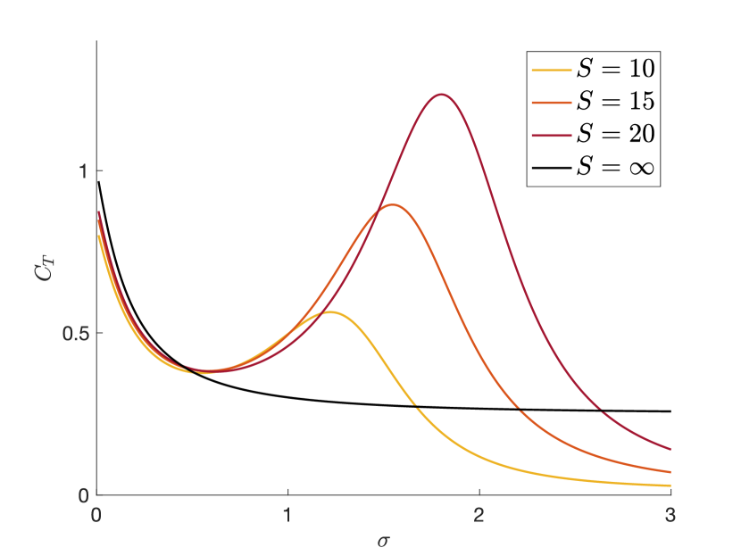
((a)) $C_{T}$

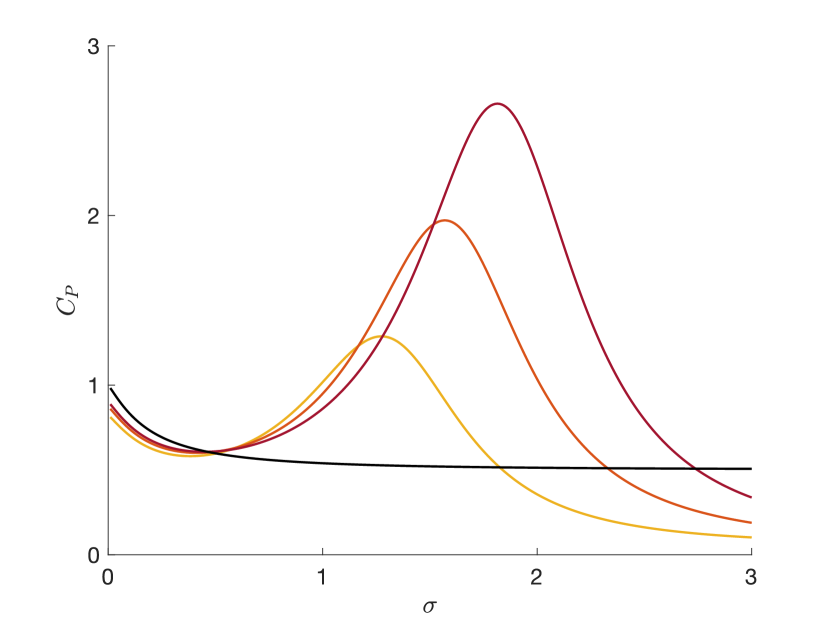
((b)) $C_{P}$

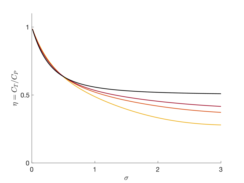
((c)) $\eta=C_{P}/C_{T}$

Figure 12: Reproduction of figure 7 in Moore (2017)

Declaration of Interests: The authors report no conflict of interest.

References

- Adams & Fish (2019) Adams, D. S. & Fish, F. E. 2019 Odontocete peduncle tendons for possible control of fluke orientation and flexibility. Journal of morphology 280 (9), 1323–1331.
- Alben (2008) Alben, S 2008 Optimal flexibility of a flapping appendage in an inviscid fluid. Journal of Fluid Mechanics 614, 355–380.
- Anderson et al. (1998) Anderson, J. M., Streitlien, K., Barrett, D. S. & Triantafyllou, M. S. 1998 Oscillating foils of high propulsive efficiency. Journal of Fluid Mechanics 360, 41–72.
- Chopra & Kambe (1977) Chopra, M. G. & Kambe, T. 1977 Hydromechanics of lunate-tail swimming propulsion. part 2. Journal of Fluid Mechanics 79 (1), 49–69.
- Dewey et al. (2013) Dewey, P A., Boschitsch, B M., Moored, K W., Stone, H A. & Smits, A J. 2013 Scaling laws for the thrust production of flexible pitching panels. Journal of Fluid Mechanics 732, 29–46.
- Faraday (1831) Faraday, M. 1831 On a peculiar class of acoustical figures; and on certain forms assumed by groups of particles upon vibrating elastic surfaces. Philosophical Transactions of the Royal Society of London (121), 299–340.
- Fish & Lauder (2006) Fish, F.E. & Lauder, G.V. 2006 Passive and active flow control by swimming fishes and mammals. Annual Review of Fluid Mechanics 38 (1), 193–224.
- Fish & Lauder (2021) Fish, F. E. & Lauder, G. V. 2021 Private communication.
- Flammang & Lauder (2008) Flammang, B. E. & Lauder, G. V. 2008 Speed-dependent intrinsic caudal fin muscle recruitment during steady swimming in bluegill sunfish, lepomis macrochirus. Journal of Experimental Biology 211 (4), 587–598.
- Floryan & Rowley (2018) Floryan, D. & Rowley, C. W. 2018 Clarifying the relationship between efficiency and resonance for flexible inertial swimmers. Journal of Fluid Mechanics 853, 271–300.
- Floryan & Rowley (2020) Floryan, D. & Rowley, C. W. 2020 Distributed flexibility in inertial swimmers. Journal of Fluid Mechanics 888, A24.
- Floryan et al. (2017a) Floryan, D., Van Buren, T., Rowley, C. W & Smits, A. J 2017a Scaling the propulsive performance of heaving and pitching foils. Journal of Fluid Mechanics 822, 386–397.
- Floryan et al. (2017b) Floryan, D., Van Buren, T. & Smits, A. J. 2017b Forces and energetics of intermittent swimming. Acta Mechanica Sinica 33 (4), 725–732.
- Garrick (1936) Garrick, I. E. 1936 Propulsion of a flapping and oscillating airfoil. In Annual Report - National Advisory Committee for Aeronautics.
- Goza et al. (2020) Goza, A., Floryan, D. & Rowley, C. 2020 Connections between resonance and nonlinearity in swimming performance of a flexible heaving plate. Journal of Fluid Mechanics 888.
- Hu et al. (2021) Hu, H., Wang, J., Wang, Y. & Dong, H. 2021 Effects of tunable stiffness on the hydrodynamics and flow features of a passive pitching panel. Journal of Fluids and Structures 100, 103175.
- Katz & Weihs (1978) Katz, J. & Weihs, D. 1978 Hydrodynamic propulsion by large amplitude oscillation of an airfoil with chordwise flexibility. Journal of Fluid Mechanics 88 (3), 485–497.
- Katz & Weihs (1979) Katz, J. & Weihs, D. 1979 Large amplitude unsteady motion of a flexible slender propulsor. Journal of Fluid Mechanics 90 (4), 713–723.
- Kumar & Tuckerman (1994) Kumar, K. & Tuckerman, L. S. 1994 Parametric instability of the interface between two fluids. Journal of Fluid Mechanics 279, 49–68.
- de Langre (2008) de Langre, E. 2008 Effects of wind on plants. Annual Review of Fluid Mechanics 40, 141–168.
- Michelin & Llewellyn Smith (2009) Michelin, S. & Llewellyn Smith, S.G. 2009 Resonance and propulsion performance of a heaving flexible wing. Physics of Fluids 21 (7), 071902.
- Miles & Henderson (1990) Miles, J. & Henderson, D. 1990 Parametrically forced surface waves. Annual Review of Fluid Mechanics 22 (1), 143–165.
- Moore (2014) Moore, M. N. J. 2014 Analytical results on the role of flexibility in flapping propulsion. Journal of Fluid Mechanics 757, 599–612.
- Moore (2015) Moore, M. N. J. 2015 Torsional spring is the optimal flexibility arrangement for thrust production of a flapping wing. Physics of Fluids 27 (9).
- Moore (2017) Moore, M. N. J. 2017 A fast Chebyshev method for simulating flexible-wing propulsion. Journal of Computational Physics 345, 792–817.
- Nayfeh & Mook (1995) Nayfeh, A. H. & Mook, D. T. 1995 Nonlinear Oscillations, chap. 5, pp. 258–364. John Wiley & Sons, Ltd.
- Paraz et al. (2016) Paraz, F, Schouveiler, L & Eloy, C 2016 Thrust generation by a heaving flexible foil: Resonance, nonlinearities, and optimality. Physics of Fluids 28 (1), 011903.
- Quinn & Lauder (2021) Quinn, D. & Lauder, G. 2021 Tunable stiffness in fish robotics: mechanisms and advantages. Bioinspiration & Biomimetics 17 (1), 011002.
- Quinn et al. (2014) Quinn, D. B., Lauder, G. V. & Smits, A. J. 2014 Scaling the propulsive performance of heaving flexible panels. Journal of Fluid Mechanics 738, 250–267.
- Schouveiler & Boudaoud (2006) Schouveiler, L. & Boudaoud, A. 2006 The rolling up of sheets in a steady flow. Journal of Fluid Mechanics 563, 71–80.
- Shi et al. (2020) Shi, Guangyu, Xiao, Qing & Zhu, Qiang 2020 Effects of time-varying flexibility on the propulsion performance of a flapping foil. Physics of Fluids 32 (12), 121904.
- Smits (2019) Smits, A. J. 2019 Undulatory and oscillatory swimming. Journal of Fluid Mechanics 874.
- Theodorsen (1935) Theodorsen, T. 1935 General theory of aerodynamic instability and the mechanism of flutter. Annual Report of the National Advisory Committee for Aeronautics 268, 413.
- Triantafyllou et al. (2000) Triantafyllou, M. S., Triantafyllou, G. S. & Yue, D. K. P. 2000 Hydrodynamics of fishlike swimming. Annual Review of Fluid Mechanics 32 (1), 33–53.
- Van Buren et al. (2017) Van Buren, T., Floryan, D., Quinn, D. & Smits, A. J. 2017 Nonsinusoidal gaits for unsteady propulsion. Phys. Rev. Fluids 2, 053101.
- Van Buren et al. (2019) Van Buren, T., Floryan, D. & Smits, A. J. 2019 Scaling and performance of simultaneously heaving and pitching foils. AIAA Journal 57 (9), 3666–3677.
- Van Buren et al. (2020) Van Buren, T., Floryan, D. & Smits, A. J 2020 Bioinspired underwater propulsors. Bioinspired Structures and Design pp. 113–139.
- Wereley (1990) Wereley, N. M. 1990 Analysis and control of linear periodically time varying systems. PhD thesis, Massachusetts Institute of Technology.
- Wu (1961) Wu, T. Y. 1961 Swimming of a waving plate. Journal of Fluid Mechanics 10 (3), 321–344.
- Wu (2011) Wu, T. Y. 2011 Fish swimming and bird/insect flight. Annual Review of Fluid Mechanics 43 (1), 25–58.