Double-slit experiment remastered

Abstract

Time-of-flight measurements of helium atoms in a double-slit experiment reported in [C. Kurtsiefer, T. Pfau, and J. Mlynek, Nature 386, 150 (1997)] are compared with the arrival times of Bohmian trajectories. This is the first qualitative comparison of a quantum mechanical arrival-time calculation with observation at the single-particle level, particularly noteworthy given the absence of a consensus in extracting time-of-flight predictions from quantum theory. We further explore a challenging double-slit experiment in which one of the slits is shut in flight.

Diffraction and interference phenomena occupy a prominent place in the phenomenology of quantum physics, Young’s double-slit experiment (DSE) being an archetypal example which, according to Feynman “has in it the heart of quantum mechanics” Feynman et al. (2011). Quantum physicists have discussed the DSE and augments thereof, e.g., the which-way Wootters and Zurek (1979); Tan and Walls (1993), or the delayed-choice DSE Wheeler (1978), with varying degrees of rigour. Several notable realisations employing single electrons Bach et al. (2013); Tonomura et al. (1989), neutrons Zeilinger et al. (1988); Gähler and Zeilinger (1991), atoms Carnal and Mlynek (1991); Kurtsiefer et al. (1997), and even macro-molecules Brand et al. (2021) have been performed. However, an essential aspect of this paradigmatic experiment amenable to observation, viz., the arrival (or detection) times of the particle at the detector, remains elusive.

While it is practically impossible to predict exactly where or when the particle will scintillate on the screen in a given experimental run, every discussion of the DSE is at least concerned with the interference fringes formed by the accumulation of single-particle impact positions depicted, e.g., in Fig. 1 (a). What tends to be overlooked, however, is that each imprinted position with screen coordinates $(x,y)$ is associated with a definite, albeit random, detection-time $t_{f}$—the time-of-flight (ToF) of the particle from the source to the screen. Figure 1 (b) gives the distribution of $t_{f}$ and the $x$-screen-coordinate of the very same detection events underlying Fig. 1 (a). Therefore, specifying the distribution of $t_{f}$ (or, better, the joint probability distribution of $x$, $y$, and $t_{f}$) is indispensable for a satisfactory account of the DSE, or any other scattering experiment for that matter. In this letter, we try to fill this gap between theory and practice.

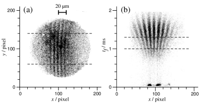
Figure 1: (a) Double-slit interference pattern observed on a screen after many single-atom detection events. (b) Joint distribution of the detection-time (or time-of-flight) $t_{f}$ and the $x$-screen-coordinate of the detection events. Impact positions of atoms arriving in the $t_{f}$ range indicated by the dashed lines in (b) were accumulated to produce (a). A fraction of very fast atoms emanating from the source cast a shadow of the slits at the bottom. (This figure is reproduced from Kurtsiefer and Mlynek (1996) with permission.)

The reader might be inclined to think that the distribution in Fig. 1 (b) corresponds to $\smash{\int\!dy\kern 1.00006pt|\psi(x,y,d,t_{f})|^{2}}$, where $\psi(x,y,z,t)$ is the particle’s wave function at time $t$ and $\smash{z=d}$ the detection plane. But this is incorrect because $|\psi(x,y,z,t)|^{2}$ is, according to Born’s rule, the distribution of positions detected at a specified time $t$, whereas what is needed is a distribution of detection times (and positions detected at such times) at a specified surface.

The measurements underlying Fig. 1 were performed by Kurtsiefer, Pfau, and Mlynek (hereafter KPM) Kurtsiefer et al. (1997); Kurtsiefer and Mlynek (1996); Pfau and Kurtsiefer (1997) in the 1990s using metastable (i.e., electronically excited) helium atoms (see below for further details). As yet, the measured arrival times and impact positions have not been compared with theory. This lacuna is not accidental. The description of the arrival times by itself is a long-standing problem with various proposed (disparate) solutions Muga and Leavens (2000); Muga et al. (1998); Das and Dürr . That there is no recognized observable for time in quantum mechanics, in contrast to position, is only partly responsible for this. While the adequacy of many existing proposals is questionable Mielnik and Torres-Vega (2005); Leavens (2002); *Mugareply; *Leavensreply; Das and Nöth (2021); Das and Struyve (2021), so far none of the suggestions have been benchmarked against experiment. To our knowledge, this work is the first comparison of this sort.

On the other hand, KPM themselves were mainly interested in the measurement (or, rather, reconstruction) of the Wigner function from ToF data Leibfried et al. (1998) theorised in earlier work Janicke and Wilkens (1995). As just indicated, standard quantum mechanics does not provide an unambiguous notion of arrival-time of a particle. Therefore, any tomographic reconstruction of the Wigner function from ToF measurements is somewhat questionable. We will not address this issue in this letter.

Instead, we will present numerical evidence showing that the statistics of impact positions and arrival times obtained by KPM can be reproduced by a pragmatic application of Bohmian mechanics. The conceptual resources provided by this theory, viz., point particles moving on definite trajectories, make it ideal for handling ToF experiments (as has long been recognized Daumer et al. (1997); Leavens (1998a, b); Grübl and Rheinberger (2002); Cushing (1995)). Bohmian trajectories are widely used in the literature for addressing arrival and tunneling-time problems, see Kazemi and Hosseinzadeh (2022); Xie et al. (2022); Leavens (1996, 1993); Douguet and Bartschat (2018); Das and Dürr (2019); *Exotic; Oriols et al. (1996); Mousavi and Golshani (2008a); Mousavi (2015); Nogami et al. (2000); Ruggenthaler et al. (2005); Pan and Home (2012); Home and Majumdar (1999); *HomeCP; Mousavi and Golshani (2008b); Demir (2022); Field (2022). Subsequently, we consider a challenging variant of the DSE, dubbed dynamic DSE, in which one of the slits is shut in flight. Finally, we conclude with some implications for the foundations of quantum mechanics.

Elements of Bohmian mechanics.

Bohmian mechanics (also called the de Broglie-Bohm theory or pilot-wave theory) is a theory about point-particles moving along trajectories that grounds the formalism and the predictions of standard quantum mechanics Bohm and Hiley (1993); Holland (1995); Dürr and Teufel (2009); Dürr et al. (2004). For a single-particle with position $\mathbf{R}$ and mass $m$, the dynamics is given by the guidance equation

$$\dot{\mathbf{R}}(t)=\frac{\hbar}{m}\kern 1.00006pt\imaginary\!\left[\frac{\boldsymbol{\nabla}\psi\big{(}\mathbf{R}(t),t\big{)}}{\psi\big{(}\mathbf{R}(t),t\big{)}}\right],$$ (1)

where $\psi(\mathbf{r},t)$ is the wave function satisfying Schrödinger’s equation with an external potential $V(\mathbf{r},t)$. The wave function never collapses in this theory. Here, the “wave/particle duality” of quantum mechanics is resolved in a trivial way: both a wave and a particle are present.

The motion of the particle is deterministic, i.e., given its initial position $\mathbf{R}(0)$ and wave function $\psi(\mathbf{r},0)$, it has a unique trajectory. However, in different experimental runs the initial positions are typically random, with distribution given by $|\psi(\mathbf{r},0)|^{2}$—the quantum equilibrium distribution. For this reason the arrival times of a particle in different runs of a scattering experiment are random, as are the locations where it strikes the detector surface.

Accounting for the DSE.

Bohmian trajectories for the DSE shown in Fig. 2 (b) are well-known; they feature invariably in expositions of Bohmian mechanics. DSE trajectories were first presented by Philippidis et al. in the late 1970s Philippidis et al. (1979) and have been reproduced various times using different methods Philippidis et al. (1982); Sanz et al. (2002); Holland and Philippidis (2003); Gondran and Gondran (2005). (Here, they are produced for the first time without simplifying assumptions on the level of the wave function.) See also Kocsis et al. (2011) for a weak measurement of average trajectories in a DSE, which resemble those of Fig. 2 (b).

The trajectories provide an almost self-explanatory account of how the interference pattern builds up on a distant screen one particle at a time. In particular, they show “how the motion of a particle, passing through just one of two holes in [a] screen, could be influenced by waves propagating through both holes. And, so influenced that the particle does not go where the waves cancel out, but is attracted to where they cooperate” (Bell, 2004, p. 191). It follows that one could have particle trajectories and still account for interference experiments, claims to the contrary notwithstanding.

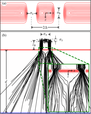
Figure 2: (a) Schematic drawing of the double-slit potential (3) for $\smash{f=1}$. The $y$-axis points out of the page, along which the potential is translationally invariant. (b) $xz$-projections of a collection of Bohmian trajectories for the DSE with initial conditions (dots) sampled randomly from the $|\psi(\mathbf{r},0)|^{2}$-distribution. Each curve tracks a particle that eventually strikes the detection plane $\smash{z=d}$ at the bottom. The following potential barrier and wave packet parameters were assumed: $\smash{V_{0}=532.5}$, $\smash{\sigma_{b}=0.075}$, $\smash{\sigma_{s}=0.25}$, $\smash{k_{x}=x_{0}=0}$, $\smash{k_{z}=10.5}$, $\smash{z_{0}=2}$, and $\smash{\sigma_{x}=3\kern 1.00006pt\sigma_{z}=0.75}$ in the units where $\smash{\hbar=m=\Delta=1}$. Inset: Characteristic non-Newtonian meandering of the Bohmian trajectories in the near-field.

For producing the Bohmian trajectories in Fig. 2 (b), we solved Schrödinger’s equation numerically with initial wave function

$$\psi(\mathbf{r},0)=\frac{e^{i(k_{x}x+k_{z}z)}}{\sqrt{\sigma_{x}\kern 1.00006pt\sigma_{y}\kern 1.00006pt\sigma_{z}}}\kern 1.00006ptG\!\left(\frac{x+x_{0}}{\sigma_{x}}\right)G\!\left(\frac{y}{\sigma_{y}}\right)G\!\left(\frac{z+z_{0}}{\sigma_{z}}\right),$$ (2)

$\smash{G(\xi)=\pi^{-1/4}\exp(-\,\xi^{2}/2)}$—a normalized Gaussian wave packet centred at $(-\kern 1.00006ptx_{0},0,-\kern 1.00006ptz_{0})$ behind the slits. The screen containing the slits was modelled by the Gaussian potential barrier

$$V=V_{0}\kern 1.00006ptG\!\left(\frac{z}{\sigma_{b}}\right)\!\left[1-S\!\left(\frac{x-\Delta}{\sigma_{s}}\right)-f\kern 1.00006ptS\!\left(\frac{x+\Delta}{\sigma_{s}}\right)\right]$$ (3)

featuring two rectangular apertures for $\smash{f=1}$, as shown in Fig. 2 (a). Here, $\smash{S(\xi)=1\raisebox{-0.86108pt}{\leavevmode\resizebox{}{6.88889pt}{\kern 1.00006pt/\kern 1.00006pt}}(1+\xi^{16})}$, $2\Delta$, $\sigma_{s}$, and $\sigma_{b}$ respectively denote the aperture function, inter-slit separation, slit-width, and the thickness of the barrier. Throughout the present work, masses, lengths and times are expressed in units of $m$, $\Delta$ and $\smash{m\Delta^{2}\kern-1.00006pt\raisebox{-0.86108pt}{\leavevmode\resizebox{}{6.88889pt}{\kern 1.00006pt/\kern 1.00006pt}}\hbar}$, respectively. (This is equivalent to setting $\smash{\hbar=m=\Delta=1}$.) The Bohmian trajectories were computed by numerically integrating the guidance equation (1) for $260$ initial positions randomly sampled from the $|\psi(\mathbf{r},0)|^{2}$-distribution. About 25% of the sampled trajectories made it through the slits giving rise to detection events. The rest (not shown in Fig. 2 (b)) were back-scattered from the potential barrier.

From pictures to predictions.

The preceding discussion suggests that an individual detection event is triggered close to the location and time-of-impact of a Bohmian trajectory. In view of this, the detection-time on a specified surface $\mathcal{D}$ (such as the plane $\smash{z=d}$) would correspond to the arrival (first passage or hitting) time of a Bohmian trajectory:

$$t_{f}(\mathbf{r}_{0})=\text{inf}\kern 1.00006pt\big{\{}\,t:\mathbf{R}(t)\in\mathcal{D}\text{ and }\mathbf{R}(0)=\mathbf{r}_{0}\,\big{\}},$$ (4)

$\mathbf{R}(t_{f})$ being the concomitant detected position on $\mathcal{D}$, as a function of the random initial condition $\mathbf{r}_{0}$—quantities that have no respective counterparts in standard quantum theory. In fact, in standard quantum theory, the detection event $\smash{(x,y,t_{f})}$ must be defined by the observation-induced collapse of the wave function, whose time of occurrence is ambiguous.

Barring special circumstances, the distribution of this detection event $\big{(}\mathbf{R}(t_{f}),t_{f}\big{)}$ is only numerically accessible. For instance, in the far-field or scattering regime, where backflow is absent, this distribution typically reduces to $j_{\perp}(\mathbf{r},t_{f})$ Kreidl et al. (2003); Daumer et al. (1997); *DDGZ96, (Das and Nöth, 2021, p. 7)—the component of the quantum flux (or probability current) density orthogonal to the surface $\mathcal{D}$. Evidently, integrating this (joint) distribution over all $t_{f}$ yields the (marginal) distribution of the detected positions alone, e.g., Fig. 1 (a). Thus arrival-time considerations are indispensable for correctly reproducing the usual interference pattern. (Note, by the way, that the quantum flux statistics is not determined by a POVM Vona et al. (2013), as would be required by the standard quantum formalism.)

Various suggested arrival-time distributions are defined with reference to a detector model, typically characterised by new phenomenological parameters, e.g., Włodarz (2002); Marchewka and Schuss (1998); *PI2; *PI3; Dubey et al. (2021); *ABC; Blanchard and Jadczyk (1998); Jurman and Nikolić (2021); Galapon et al. (2005); *CTOA; *CTOAerror. In our case, a very compelling qualitative agreement with the experimental data is obtained by disregarding the micro-physics of the detector altogether, and without introducing any free parameters. While a more detector-aware Bohmian analysis could be envisaged, this is easier said than done, and our results indicate that this may not even be necessary.

Specifics of the KPM experiment.

In Kurtsiefer et al. (1997), the metastable helium atoms (denoted He^*) are sourced from a gas-discharge tube by firing a $15\,\mu\text{s}$ pulse of electric current. A few spurious fast-moving atoms along with slower atoms with velocities ranging between $\smash{1-3\times 10^{3}\,\text{ms}^{-1}}$ (Pfau and Kurtsiefer, 1997, Fig. 4) are produced by the source. The ejected atoms pass through a skimmer and are collimated by a $\smash{5\,\mu\text{m}}$-wide slit. Further downstream, they encounter a microfabricated double-slit structure of inter-slit separation $\smash{2\Delta=8\,\mu\text{m}}$ and slit-width $\sigma_{s}=1\,\mu\text{m}$, eventually striking the detector plate at $d$.

He^* atoms eject secondary electrons upon hitting the conductive surface of the detector—a process assumed to take place on a time scale of $10^{-12}\,\text{s}$. These electrons are carefully imaged onto a single-electron detection unit based on a chevron assembly of multichannel plates Kurtsiefer and Mlynek (1996). The spatial (temporal) resolution achieved with this detector is on the order of $500\,\text{nm}$ ($100\,\text{ns}$).

For three different slit-screen separations $d$, KPM recorded the detection events $(x,y,t_{f})$ of individual atoms by repeatedly firing the source. Their observations are shown in Fig. 3 (left panel). Notice that the fast atoms produce a “geometrical shadow” of the slits at the bottom of each figure (Kurtsiefer et al., 1997, p. 151).

A numerical treatment of the KPM experiment.

Assuming an initial Gaussian wave packet (2), we solved Schrödinger’s equation with the double-slit potential (3). The wave function then determines the particle velocity in the guidance equation (1). Numerically integrating Eq. (1) for $5\times 10^{4}$ initial conditions randomly sampled from the $|\psi(\mathbf{r},0)|^{2}$ distribution, we recorded the impact positions $\big{(}X(t_{f}),Y(t_{f})\big{)}$ and arrival times $t_{f}$ of Bohmian trajectories arriving at $\smash{z=d}$. Histograms of obtained $t_{f}$ and $X(t_{f})$ are presented in Fig. 3 (right panel).

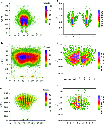
Figure 3: Joint distributions of arrival times and $x$-screen coordinates for different slit-screen separations. Left panel: Experimental data for He^* atoms with $\smash{d=148\,\text{mm}}$ (a), $\smash{d=248\,\text{mm}}$ (b), and $\smash{d=1,950\,\text{mm}}$ (c) (reproduced from Kurtsiefer et al. (1997) with permission). Here, $\smash{t_{d}=(d/L)\,t_{f}}$ is a “scaled ToF”, where $L$ is the source-to-screen separation. Right panel: Numerical data generated from Bohmian trajectory impacts for $\smash{V_{0}=665.7}$, $\smash{\sigma_{b}=0.125}$, $\smash{\sigma_{s}=0.5}$, $\smash{k_{x}=-\,0.5}$, $\smash{k_{z}=15.7}$, $\smash{z_{0}=4}$, $\smash{x_{0}=-\,0.13}$, $\smash{\sigma_{x}=2.25}$, $\smash{\sigma_{z}=0.25}$, with $\smash{d=0.9}$ (d), $\smash{d=9}$ (e), and $\smash{d=15}$ (f), in the units where $\smash{\hbar=m=\Delta=1}$.

We made a few assumptions in order to enable numerics: (A) The large spatial extent of KPM’s experimental set-up prevents a straightforward solution of the time-dependent Schrödinger equation, therefore we chose wave packet and potential barrier parameters that have similar relative values in our units. (B) Our particles start directly behind the double slits, rather than at the source. Since $k_{z}$ is very large, all particles have practically the same transit-time from the source to the slits, which can therefore be ignored in computing the total $t_{f}$ without affecting the shape of the arrival-time distribution significantly. It is the double-slit potential (3) which entangles the motions in the $x$ and $z$ directions correlating the particle arrival-times with the $x$-screen coordinate of their impact positions, captured in Fig. 2. (C) Finally, we have employed the same initial wave function for each run of the DSE, even though the discharge tube yields a statistical mixture of wave packets of different longitudinal velocities. Lacking additional details of the KPM discharge source, we chose this simpler treatment.

Despite these simplifications, we do find a good qualitative agreement between the raw data reported by KPM and our numerical calculations in Fig. 3. This indicates that the obtained statistics are generic and are not too sensitive to the aspects we have glossed over. Arguably, a better characterisation of the source in the analysis or more accurate numerical simulations can only make the agreement better. Also, our results further underscore the point (discussed earlier) that a microscopic account of the detector for predicting the measured arrival times is certainly unnecessary for producing results comparable in accuracy to the usual interference pattern discussed in textbooks.

Dynamic DSE.

In what follows, we set

$$f=\frac{1}{2}\kern 1.00006pt\bigg{\{}\kern 1.00006pt1+\tanh\kern-1.00006pt\big{[}\gamma\kern 1.00006pt(t_{c}-t)\big{]}\kern 1.00006pt\bigg{\}},$$ (5)

in (3), which causes the slit centred at $\smash{x=-\kern 1.00006pt\Delta}$ to gradually close in time. In particular, for $\smash{t\gg(\ll)\,t_{c}}$, $\smash{f\approx 0\,(1)}$ implying a completely closed (open) slit. (A dynamically controlled DSE is well-amenable to present-day technology Bach et al. (2013).) Scatter plots of $\big{(}X(t_{f}),t_{f}\big{)}$ for this dynamic DSE are plotted in Fig. 4 for two values of $\gamma$; a large (small) $\gamma$ implies a fast (slow) closing of the slit. The closing time $t_{c}$ is chosen close to the time at which the peak of the wave packet strikes $\smash{z=0}$, i.e., $\smash{z_{0}\raisebox{-0.86108pt}{\leavevmode\resizebox{}{6.88889pt}{\kern 1.00006pt/\kern 1.00006pt}}k_{z}}$. Evidently, a smaller number of trajectories pass through the closing slit. Furthermore, the interference fringes become less pronounced for $\smash{t_{f}\gg t_{c}}$, as would be expected for single-slit diffraction.

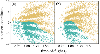
Figure 4: Scatter plot of $\smash{\approx 10^{4}}$ Bohmian trajectories arriving at $\smash{d=10}$ over time for the dynamic DSE, where the slit centred at $\smash{x=-\kern 1.00006pt\Delta}$ ($\smash{=-\kern 1.00006pt1}$ in our units) is closed in flight around time $\smash{t_{c}=0.25}$: (a) Fast switching $\smash{\gamma=100}$, (b) Slow switching $\smash{\gamma=20}$. Data points for trajectories passing through the closing (open) slit are rendered in blue (beige). Potential barrier and initial wave packet parameters are same as Fig. 2.

Concluding remarks.

The computation of the probability distribution of arrival or detection times of quantum particles is one of the last areas where experts disagree about what quantum mechanics should predict. While a cornucopia of different ToF distributions exists in the literature, one rarely finds a discussion of the joint distribution of impact positions and arrival times studied in this work (and measured in the KPM experiment). In this letter, we have presented a Bohmian calculation of such distributions, obtaining a compelling qualitative agreement with the KPM measurements.

While Bohmian mechanics, owing to the well-defined concepts of point-particles and trajectories embedded in it, is readily suited for explaining the results of such ToF experiments, it is as yet unclear how alternative quantum theories, e.g., spontaneous/objective collapse and many-worlds theories, among others, would deal with the same in a practicable way.

It must be emphasized that the Bohmian trajectories serve not only to anchor one’s intuition, but also to provide theoretical resources for interpreting laboratory ToF experiments that otherwise canonically rely on Newtonian concepts. The applicability of such concepts is often questionable, e.g., in discussing tunneling situations (see also Das and Struyve (2021)). Given that ToF measurements are routinely performed to measure/reconstruct physical quantities of interest, a first principles underpinning of ToF measurements becomes all the more necessary.

To make progress with this question, we recommend that ToF resolved DSEs and dynamic variants thereof, as described in this work, should be performed with present-day technology to achieve a quantitative experiment-to-theory comparison in the future. A particular improvement would be better control of the initial wave function of the particle, e.g., sourcing the particle from an ion trap post-cooling Stopp et al. (2022), or using field-emission-tip electron wave packets à la Jones et al. (2016), both of which offer better initial wave packet control compared to a gas-discharge source.

References

- Feynman et al. (2011) R. Feynman, R. Leighton, and M. Sands, The Feynman Lectures on Physics, Quantum Mechanics Vol. III (Basic Books, 2011).
- Wootters and Zurek (1979) W. K. Wootters and W. H. Zurek, Phys. Rev. D 19, 473 (1979).
- Tan and Walls (1993) S. M. Tan and D. F. Walls, Phys. Rev. A 47, 4663 (1993).
- Wheeler (1978) J. A. Wheeler, in Mathematical Foundations of Quantum Theory, edited by A. Marlow (Academic Press, 1978) pp. 9–48.
- Bach et al. (2013) R. Bach, D. Pope, S.-H. Liou, and H. Batelaan, New J. Phys. 15, 033018 (2013).
- Tonomura et al. (1989) A. Tonomura, J. Endo, T. Matsuda, T. Kawasaki, and H. Ezawa, Am. J. Phys. 57, 117 (1989).
- Zeilinger et al. (1988) A. Zeilinger, R. Gähler, C. G. Shull, W. Treimer, and W. Mampe, Rev. Mod. Phys. 60, 1067 (1988).
- Gähler and Zeilinger (1991) R. Gähler and A. Zeilinger, Am. J. Phys. 59, 316 (1991).
- Carnal and Mlynek (1991) O. Carnal and J. Mlynek, Phys. Rev. Lett. 66, 2689 (1991).
- Kurtsiefer et al. (1997) C. Kurtsiefer, T. Pfau, and J. Mlynek, Nature 386, 150 (1997).
- Brand et al. (2021) C. Brand, S. Troyer, C. Knobloch, O. Cheshnovsky, and M. Arndt, Am. J. Phys. 89, 1132 (2021).
- Kurtsiefer and Mlynek (1996) C. Kurtsiefer and J. Mlynek, Appl. Phys. B 64, 85 (1996).
- Pfau and Kurtsiefer (1997) T. Pfau and C. Kurtsiefer, J. Mod. Opt. 44, 2551 (1997).
- Muga and Leavens (2000) J. G. Muga and C. R. Leavens, Phys. Rep. 338, 353 (2000).
- Muga et al. (1998) J. Muga, R. Sala, and J. Palao, Superlattices and Microstructures 23, 833 (1998).
- (16) S. Das and D. Dürr, “Benchmarking quantum arrival time distributions using a back-wall,” in preparation.
- Mielnik and Torres-Vega (2005) B. Mielnik and G. Torres-Vega, Concepts of Physics. II, 81 (2005).
- Leavens (2002) C. R. Leavens, Phys. Lett. A 303, 154 (2002).
- Egusquiza et al. (2003) I. Egusquiza, J. Muga, B. Navarro, and A. Ruschhaupt, Phys. Lett. A 313, 498 (2003).
- Leavens (2005) C. R. Leavens, Phys. Lett. A 345, 251 (2005).
- Das and Nöth (2021) S. Das and M. Nöth, Proc. R. Soc. A. 477, 20210101 (2021).
- Das and Struyve (2021) S. Das and W. Struyve, Phys. Rev. A 104, 042214 (2021).
- Leibfried et al. (1998) D. Leibfried, T. Pfau, and C. Monroe, Phys. Today 51, 22 (1998).
- Janicke and Wilkens (1995) U. Janicke and M. Wilkens, J. Mod. Opt. 42, 2183 (1995).
- Aharonov et al. (1998) Y. Aharonov, J. Oppenheim, S. Popescu, B. Reznik, and W. G. Unruh, Phys. Rev. A 57, 4130 (1998).
- Daumer et al. (1997) M. Daumer, D. Dürr, S. Goldstein, and N. Zanghì, J. Stat. Phys. 88, 967 (1997).
- Leavens (1998a) C. Leavens, Phys. Rev. A 58, 840 (1998a).
- Leavens (1998b) C. R. Leavens, Superlattices and Microstructures 23, 795 (1998b).
- Grübl and Rheinberger (2002) G. Grübl and K. Rheinberger, J. Phys. A: Math. Gen. 35, 2907 (2002).
- Cushing (1995) J. T. Cushing, Found. Phys. 25, 269 (1995).
- Kazemi and Hosseinzadeh (2022) M. Kazemi and V. Hosseinzadeh, arXiv:2208.01325 (2022).
- Xie et al. (2022) W. Xie, M. Li, Y. Zhou, and P. Lu, Phys. Rev. A 105, 013119 (2022).
- Leavens (1996) C. R. Leavens, “The “tunneling-time problem” for electrons,” in Bohmian Mechanics and Quantum Theory: An Appraisal, edited by J. T. Cushing, A. Fine, and S. Goldstein (Springer Netherlands, Dordrecht, 1996) pp. 111–129.
- Leavens (1993) C. Leavens, Phys. Lett. A 178, 27 (1993).
- Douguet and Bartschat (2018) N. Douguet and K. Bartschat, Phys. Rev. A 97, 013402 (2018).
- Das and Dürr (2019) S. Das and D. Dürr, Sci. Rep. 9, 2242 (2019).
- Das et al. (2019) S. Das, M. Nöth, and D. Dürr, Phys. Rev. A 99, 052124 (2019).
- Oriols et al. (1996) X. Oriols, F. Martín, and J. Suñé, Phys. Rev. A 54, 2594 (1996).
- Mousavi and Golshani (2008a) S. V. Mousavi and M. Golshani, Phys. Scr. 78, 035007 (2008a).
- Mousavi (2015) S. V. Mousavi, Phys. Scr. 90, 095001 (2015).
- Nogami et al. (2000) Y. Nogami, F. Toyama, and W. van Dijk, Phys. Lett. A 270, 279 (2000).
- Ruggenthaler et al. (2005) M. Ruggenthaler, G. Grübl, and S. Kreidl, J. Phys. A: Math. Gen. 38, 8445 (2005).
- Pan and Home (2012) A. K. Pan and D. Home, Int. J. Theor. Phys 51, 374–389 (2012).
- Home and Majumdar (1999) D. Home and A. S. Majumdar, Found. Phys. 29, 721 (1999).
- Majumdar and Home (2002) A. S. Majumdar and D. Home, Phys. Lett. A 296, 176 (2002).
- Mousavi and Golshani (2008b) S. V. Mousavi and M. Golshani, J. Phys. A: Math. Theor. 41, 375304 (2008b).
- Demir (2022) D. Demir, Phys. Rev. A 106, 022215 (2022).
- Field (2022) G. E. Field, Euro. Jnl. Phil. Sci. 12 (2022).
- Bohm and Hiley (1993) D. Bohm and B. J. Hiley, The Undivided Universe: An Ontological Interpretation of Quantum Theory (Routledge, London and New York, 1993).
- Holland (1995) P. R. Holland, The quantum theory of motion: an account of the de Broglie-Bohm causal interpretation of quantum mechanics (Cambridge university press, 1995).
- Dürr and Teufel (2009) D. Dürr and S. Teufel, Bohmian Mechanics: The Physics and Mathematics of Quantum Theory (Springer-Verlag, Berlin, 2009).
- Dürr et al. (2004) D. Dürr, S. Goldstein, and N. ZanghÌ, J. Stat. Phys. 116, 959 (2004).
- Philippidis et al. (1979) C. Philippidis, C. Dewdney, and B. Hiley, IL Nuov Cim B 52, 15 (1979).
- Philippidis et al. (1982) C. Philippidis, D. Bohm, and R. D. Kaye, IL Nuov Cim B 71, 75 (1982).
- Sanz et al. (2002) A. S. Sanz, F. Borondo, and S. Miret-Artés, J. Phys.: Condens. Matter 14, 6109 (2002).
- Holland and Philippidis (2003) P. Holland and C. Philippidis, Phys. Rev. A 67, 062105 (2003).
- Gondran and Gondran (2005) M. Gondran and A. Gondran, Am. J. Phys. 73, 507 (2005).
- Kocsis et al. (2011) S. Kocsis et al., Science 332, 1170 (2011).
- Bell (2004) J. S. Bell, Speakable and Unspeakable in Quantum Mechanics: Collected Papers on Quantum Philosophy (Cambridge University Press, 2004).
- Landau and Lifshitz (1977) L. D. Landau and E. M. Lifshitz, Quantum Mechanics: Nonrelativistic theory, 3rd ed., Course of Theoretical Physics, Vol. 3 (Pergamon Press, Moscow, 1977).
- Kreidl et al. (2003) S. Kreidl, G. Grübl, and H. G. Embacher, J. Phys. A: Math. Gen. 36, 8851 (2003).
- Daumer et al. (1996) M. Daumer, D. Dürr, S. Goldstein, and N. Zanghì, Lett. Math. Phys. 38, 103 (1996).
- Vona et al. (2013) N. Vona, G. Hinrichs, and D. Dürr, Phys. Rev. Lett. 111, 220404 (2013).
- Włodarz (2002) J. J. Włodarz, Phys. Rev. A 65, 044103 (2002).
- Marchewka and Schuss (1998) A. Marchewka and Z. Schuss, Phys. Lett. A 240, 177 (1998).
- Marchewka and Schuss (2001) A. Marchewka and Z. Schuss, Phys. Rev. A 63, 032108 (2001).
- Marchewka and Schuss (2002) A. Marchewka and Z. Schuss, Phys. Rev. A 65, 042112 (2002).
- Dubey et al. (2021) V. Dubey, C. Bernardin, and A. Dhar, Phys. Rev. A 103, 032221 (2021).
- Tumulka (2022) R. Tumulka, Ann. Phys. 442, 168910 (2022).
- Blanchard and Jadczyk (1998) P. Blanchard and A. Jadczyk, Int. J. Theor. Phys. 37, 227 (1998).
- Jurman and Nikolić (2021) D. Jurman and H. Nikolić, Phys. Lett. A 396, 127247 (2021).
- Galapon et al. (2005) E. A. Galapon, R. Caballar, and R. Bahague, Phys. Rev. A 72, 062107 (2005).
- Galapon et al. (2004) E. A. Galapon, R. F. Caballar, and R. T. B. Jr, Phys. Rev. Lett. 93, 180406 (2004).
- Galapon et al. (2008) E. A. Galapon, R. F. Caballar, and R. T. B. Jr, Phys. Rev. Lett. 101, 169901 (2008).
- Tastevin and Laloë (2018) G. Tastevin and F. Laloë, Eur. Phys. J. D 72, 033018 (2018).
- Wiseman (1998) H. M. Wiseman, Phys. Rev. A 58, 1740 (1998).
- Lazarovici and Hubert (2019) D. Lazarovici and M. Hubert, Sci Rep 9, 470 (2019).
- Nitta and Kudo (2008) H. Nitta and T. Kudo, Phys. Rev. A 77, 014102 (2008).
- Sainadh et al. (2020) U. S. Sainadh, R. T. Sang, and I. V. Litvinyuk, J. Phys. Photonics 2, 042002 (2020).
- Ramos et al. (2020) R. Ramos, D. Spierings, I. Racicot, and A. M. Steinberg, Nature 583, 529 (2020).
- Stopp et al. (2022) F. Stopp, H. Lehec, and F. Schmidt-Kaler, Quantum Sci. Technol. (2022).
- Jones et al. (2016) E. Jones, M. Becker, J. Luiten, and H. Batelaan, Laser Photon Rev. 10, 214 (2016).